MEASUREMENTS OF THE MOLAR HEAT

CAPACITY AND THE MOLAR EXCESS ENTHALPY

FOR VARIOUS ALKANOLAMINES IN AQUEOUS

SOLUTIONS

A Thesis

Submitted to the Faculty of Graduate Studies and Research

In Partial Fulfillment of the Requirements

For the Degree of

Master of Applied Science

In

Industrial Systems Engineering

University of Regina

By

AhmadrezaNezamloo

Regina, Saskatchewan

July, 2013

2013:A.R.Nezamloo

UNIVERSITY OF REGINA

FACULTY OF GRADUATE STUDIES AND RESEARCH

SUPERVISORY AND EXAMINING COMMITTEE

Ahmadreza Nezamloo, candidate for the degree of Master of Applied Science in Industrial Systems Engineering, has presented a thesis titled, Measurements of the Molar Heat Capacity and the Molar Excess Enthalpy for Various Alkanolamines in Aqueous Solutions, in an oral examination held on July 24, 2013. The following committee members have found the thesis acceptable in form and content, and that the candidate demonstrated satisfactory knowledge of the subject material. External Examiner: Dr. Shahid Azam, Environmental Systems Engineering

Supervisor: Dr. Amr Henni, Industrial Systems Engineering

Committee Member: Dr. Mohamed Ismail, Industrial Systems Engineering

Committee Member: Dr. Mohamed El-Darieby, Software Systems Engineering

Chair of Defense: Dr. Larena Hoeber, Faculty of Kinesiology & Health Studies

i

Abstract

The purpose of this study is to determine the molar heat capacity (Cp) and molar

excess enthalpy for 4-Ethylmorpholine, 2-(Isopropylamino)ethanol, 2-

(Diisopropylamino)ethanol, 3-Dimethylamino-1-propanol(3-DEAP), and1-

Dimethylamino-2-propanol (1-DEAP) in aqueous solutions by means of a C80 heat flow

calorimeter over the entire range of mole fractions at different temperatures. The heat

capacity measurements were carried out from 303.15K to 353.15K, whereas the excess

enthalpies were measured at 298.15, 313.15, and 333.15K. An estimated uncertainty of

1% was found in the measured amount of the molar excess enthalpy as well as heat

capacity.

Among the five selected alkanolamines, 2-DPAE possessed the highest value in

terms of molar heat capacity whereas 4-EMP had the lowest value. The values of heat

capacities are dominated by –CH3. In this study, the experimental values of molar heat

capacities were correlated using the Redlich-Kister Equation.

Solution theory and group contribution modelslike NRTL (Non-random Two-

liquid), UNIQUAC (Universal-Quasi chemical), and UNIFAC (Universal Functional

activity coefficient) were used to model the experimental values of the molar excess

enthalpies. Among the three above-mentioned models, the modified UNIFAC

(Dortmund) was the most accurate for predicting and representing the values of molar

excess enthalpies.

The present study shows the value of molar excess enthalpies for the five selected

amines are dominated by –CH3 group contribution and most importantly by the steric

ii

hindrance of the amine. The molar excess enthalpy increases in the negative side with

more access of water molecules to the nitrogen atom.

The negative value of molar excess enthalpies decreases as the temperature increases.

This study has shown that the interaction between the hydrogen of water and amine

group plays a significant role in the magnitude of the molar excess enthalpies of the five

selected alkanolamines.

iii

Acknowledgments

I wish to express my sincere gratitude to my supervisor, Dr. AmrHenni, for his advice,

encouragement, and financial assistance throughout my study. I would like to thank Dr.

Mehrandezh, my co-supervisor. I would not have been able to complete this research

without the unconditional support of my family, and friends.

Finally, I would like to acknowledge funding through the faculty of graduate studies and

research as well.

iv

Table of Contents

Abstract................................................................................................................. i

Acknowledgments ................................................................................................ iii

Table of Contents ................................................................................................iv

List of Figures ......................................................................................................vi

List of Tables .......................................................................................................ix

NOMENCLATURE .............................................................................................. xii

CHAPTER 1: INTRODUCTION ........................................................................... 1

1.0 Purpose ...................................................................................................... 5

1.1 Scope ......................................................................................................... 6

1.1.1 4-Ethylmorpholine ................................................................................ 6

1.1.2 2-(Isopropylamino)ethanol .................................................................... 6

1.1.3 2-(Diisopropylamino)ethanol ................................................................ 7

1.1.4 3-Dimethylamino-1-propanol ............................................................... 7

1.1.5 1-Dimethylamino-2-propanol ................................................................ 7

CHAPTER 2: LITERATURE REVIEW ................................................................. 9

2.1. Calorimeter Methods ............................................................................... 11

2.1.1. Adiabatic Calorimeter ........................................................................ 11

2.1.2. Isothermal Calorimeter ...................................................................... 11

2.1.3. Isothermal Dilution Calorimeter ......................................................... 12

2.1.4 Flow Calorimeter ................................................................................ 12

2.2. Predictions and Correlation Approaches ................................................. 13

2.2.1. Experimental Expressions ................................................................. 13

2.2.2. Methods for Solution Theory ............................................................. 14

2.2.3. Methods of Group Contribution ......................................................... 16

2.3. Non-Random Two Liquid model (NRTL) ................................................. 17

2.4. Universal Quasi-Chemical Theory Model ................................................ 19

2.5. Universal Functional Activity Coefficient (Dortmund) model .................... 21

2.6 Finding the parameters ............................................................................. 25

CHAPTER 3: EXPERIMENTAL METHODS ...................................................... 26

v

3.1. Equipment ............................................................................................... 26

3.2. Calibration ............................................................................................... 30

3.3. Measurement of Cp .................................................................................. 35

3.3.1. Methods for measurement of Cp ........................................................ 35

3.4. Measurement of Heat of Mixing ............................................................... 39

3.5. Errors ....................................................................................................... 42

3.6. Preparation of solution ............................................................................. 42

3.7. Verification of the C80 calorimeter ........................................................... 43

CHAPTER 4: RESULTS AND DISCUSSION .................................................... 50

4.1 Molar Heat Capacity Measurements ........................................................ 50

4.1.1 4-Ethylmorpholine(4-EMP) ................................................................. 50

4.1.2. 2-(Isopropylamino)ethanol(2-IPAE) ................................................... 56

4.1.3. 2-(Diisopropylamino)ethanol(2-DPAE) .............................................. 60

4.1.4. 3-Dimethylamino-1-propanol(3-DEAP) .............................................. 64

4.1.5. 1-Dimethylamino-2-propanol (1-DEAP) ............................................. 68

4.2. Comparison of results for Cp values ........................................................ 72

4.3. Molar excess enthalpy measurements .................................................... 73

4.3.1. 4-Ethylmorpholine(4-EMP) ................................................................ 74

4.3.2. 2-(Isopropylamino)ethanol(2-IPAE) ................................................... 79

4.3.3. 2-(Diisopropylamino)ethanol(2-DPAE) .............................................. 84

4.3.4. 3-Dimethylamino-1-propanol(3-DEAP) .............................................. 89

4.3.5. 1-Dimethylamino-2-propanol (1-DEAP) ............................................. 94

CHAPTER 5: CONCLUSION ........................................................................... 100

REFERENCES ................................................................................................ 103

APPENDIX ....................................................................................................... 111

vi

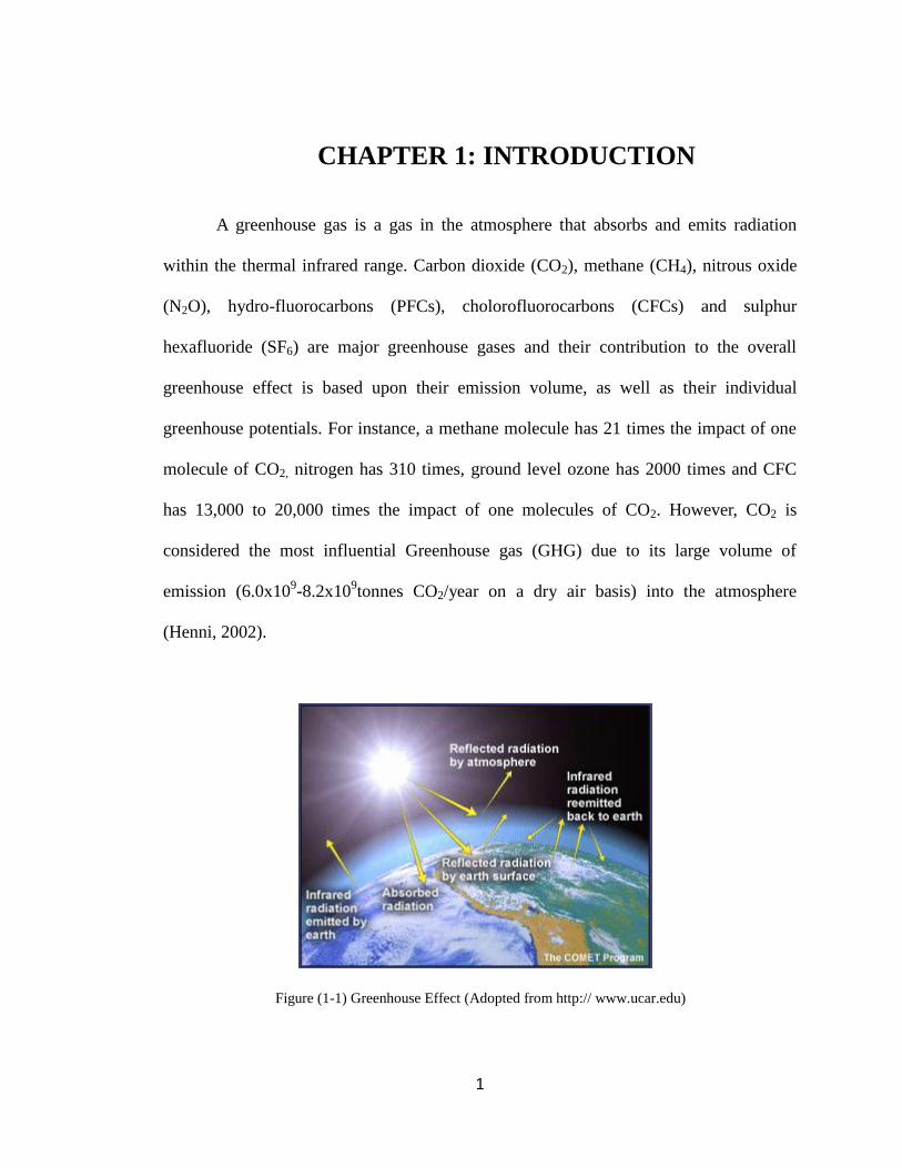
List of Figures Figure (1-1) Greenhouse Effect (Adopted from http:// www.ucar.edu) ................. 1

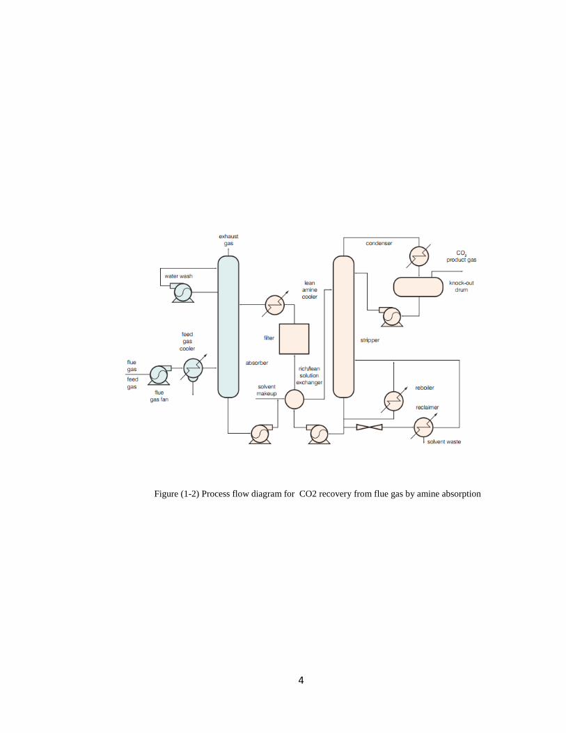
Figure (1-2) Process flow diagram for CO2 recovery from flue gas by amine

absorption ............................................................................................................ 4

Figure (3-1) Sectional view of the C80 Flow Calorimeter ................................... 29

Figure (3-1a) Sensitivity calibration curve .......................................................... 33

Figure (3-1b) Temperature calibration with indium at 0.4 K/min of scanning rate

........................................................................................................................... 34

Figure (3-2) Three steps method for determination of molar heat capacity signals

........................................................................................................................... 37

Figure (3-2a) Standard cell for measurement of the molar heat capacity .......... 38

Figure (3-3) Membrane mixing for the molar excess enthalpy measurement .... 40

Figure (3-4) Molar excess enthalpy graph ......................................................... 41

Figure (3-5) Comparison of the molar heat capacity data for pure MEA ............ 48

Figure (3-6) Comparison of the molar heat capacity data for pure MDEA ......... 48

Figure (3-7) Molar excess enthalpies for MDEA and water at 313.15 K ............ 49

Figure (4-1) Molar heat capacity of 4-EMP in aqueous solution at different

temperatures ...................................................................................................... 52

Figure (4-2) Molar excess heat capacity of 4-EMP in aqueous solution ............ 52

Figure (4-3) Reduced molar excess heat capacity for 4-Ethylmorpholine

solutions............................................................................................................. 54

Figure (4-4) Molar heat capacity of 2-IPAE in aqueous solution at different

temperatures ...................................................................................................... 57

Figure (4-5) Molar excess heat capacity of 2-IPAE in aqueous solution ............ 58

Figure (4-6) Reduced molar excess heat capacity for 2-(Isopropylamino)ethanol

solutions............................................................................................................. 58

Figure (4-7) Molar heat capacity of 2-(Diisopropylamino)ethanol at different

temperatures ...................................................................................................... 61

Figure (4-8) Molar excess heat capacity of 2-(Diisopropylamino)ethanol in

aqueous solution ................................................................................................ 62

Figure (4-9) Reduced molar excess heat capacity for 2-

(Diisopropylamino)ethanol solutions .................................................................. 62

Figure (4-9a) Molar heat capacity of 3-Dimethylamino-1-propanol at different

temperatures ...................................................................................................... 65

Figure (4-10) Molar excess heat capacity of 3-Dimethylamino-1-propanol in

aqueous solution ................................................................................................ 66

Figure (4-11) Reduced molar excess heat capacity for 3-Dimethylamino-1-

propanol solutions .............................................................................................. 66

Figure (4-12) Molar heat capacity of 1-Dimethylamino-2-propanol at different

temperatures ...................................................................................................... 69

vii

Figure (4-13) Molar excess heat capacity of 1-Dimethylamino-2-propanol in

aqueous solution ................................................................................................ 70

Figure (4-14) Reduced molar excess heat capacity for 1-Dimethylamino-2-

propanol solutions .............................................................................................. 70

Figure (4-15) Comparison of Cp values for five alkanolamines: 4-EMP,2-IPAE,2-

DPAE,3-DEAP,1-DEAP ..................................................................................... 73

Figure (4-16) Molar excess enthalpies for mixture of 4-EMP+ Water ............... 77

Figure (4-17) Molar excess enthalpy of 4-EMP+water represented by NRTL

model ................................................................................................................. 77

Figure (4-18) Molar excess enthalpy of 4-EMP+water represented by UNIQUAC

model ................................................................................................................. 77

Figure (4-19) Molar excess enthalpy of 4-EMP+water represented by UNIFAC

model ................................................................................................................. 78

Figure (4-19a) Molar excess enthalpies for mixture of 2-IPAE+ Water ............. 81

Figure (4-20) Molar excess enthalpy of 2-IPAE+water represented by NRTL

model ................................................................................................................. 82

Figure (4-21) Molar excess enthalpy of 2-IPAE+water represented by UNIQUAC

model ................................................................................................................. 82

Figure (4-22) Molar excess enthalpy of 2-IPAE+water represented by UNIFAC

model ................................................................................................................. 83

Figure (4-23) Molar excess enthalpies for mixture of 2-DPAE+ Water ............. 86

Figure (4-24) Molar excess enthalpy of 2-DPAE+water represented by NRTL

model ................................................................................................................. 86

Figure (4-25) Molar excess enthalpy of 2-DPAE+water represented by

UNIQUAC model ............................................................................................... 87

Figure (4-26) Molar excess enthalpy of 2-DPAE+water represented by UNIFAC

model ................................................................................................................. 88

Figure (4-27) Molar excess enthalpies for mixture of 3-DEAP+ Water ............. 90

Figure (4-28) Molar excess enthalpy of 3-DEAP+water represented by NRTL

model ................................................................................................................. 91

Figure (4-29) Molar excess enthalpy of 3-DEAP+water represented by

UNIQUAC model ............................................................................................... 91

Figure (4-30) Molar excess enthalpy of 3-DEAP+water represented by UNIFAC

model ................................................................................................................. 93

Figure (4-31) Molar excess enthalpies for mixture of 1-DEAP+ Water ............. 96

Figure (4-32) Molar excess enthalpy of 1-DEAP+water represented by NRTL

model ................................................................................................................. 96

Figure (4-33) Molar excess enthalpy of 1-DEAP+water represented by

UNIQUAC model ............................................................................................... 97

Figure (4-34) Molar excess enthalpy of 1-DEAP+water represented by UNIFAC

model ................................................................................................................. 98

viii

Figure (4-35) Comparison of the molar excess enthalpies of the five selected

alkanolamines at 333.15 K................................................................................. 99

Figure (4-36) Comparison of the molar excess enthalpies of different

alkanolamines .................................................................................................... 99

ix

List of Tables Table 1.1. Specifications of the selected alkanolamines ...................................... 8

Table 2.2. Main groups and the corresponding van der Waals quantities for the

modified UNIFAC ............................................................................................... 24

Table 3.1. Sensitivity constants ......................................................................... 31

Table 3.2. Temperature Correction Coefficients ................................................ 32

Table 3.3. Molar Heat Capacity Data of MEA and MDEA .................................. 45

Table 3.4. Molar excess enthalpies for MEA system ......................................... 46

Table 3.5. Molar excess enthalpies for MDEA system ....................................... 47

Table 4.1. Redlich-Kister Equation coefficients for the molar excess heat

capacity for 4-Ethylmorpholine (4-EMP) .................................................... 55

Table 4.2. Redlich-Kister Equation coefficients for the molar excess heat

capacity for 2-IPAE ..................................................................................... 59

Table 4.3. Redlich-Kister Equation coefficients for the molar excess heat

capacity for 2-DPAE ................................................................................... 63

Table 4.4. Redlich-Kister Equation coefficients for the molar excess heat

capacity for 3-DEAP ................................................................................... 67

Table 4.5. Redlich-Kister Equation coefficients for the molar excess heat

capacity for 1-DEAP ................................................................................... 71

Table 4.6. Fitting coefficients for Redlich-Kister Equation for the molar excess

enthalpy for 4-EMP+water at three temperatures .............................................. 76

Table 4.7. Parameters for NRTL and UNIQUAC models for the molar excess

enthalpy data of aqueous 4-EMP for three different temperatures (298.15,

313.15, and 33.15 K) ......................................................................................... 78

Table 4.8. ........................................................................................................... 79

Table 4.9. Interaction parameters for UNIFAC model for the molar excess

enthalpy data of aqueous 4-EMP for three different temperatures (298.15,

313.15, and 33.15 K) ......................................................................................... 79

Table 4.10. Fitting coefficients for Redlich-Kister Equation for the molar excess

enthalpy for 2-IPAE+water at three temperatures .............................................. 81

Table 4.11. Parameters for NRTL and UNIQUAC models for the molar excess

enthalpy data of aqueous 2-IPAE for three different temperatures (298.15,

313.15, and 33.15 K) ......................................................................................... 83

Table 4.12. Interaction parameters for UNIFAC model for the molar excess

enthalpy data of aqueous 2-IPAE for three different temperatures (298.15,

313.15, and 33.15) K ......................................................................................... 84

Table 4.13. Fitting coefficients for Redlich-Kister Equation for the molar excess

enthalpy for 2-DPAE+water at three temperatures ............................................ 85

x

Table 4.14. Parameters for NRTL and UNIQUAC models for the molar excess

enthalpy data of aqueous 2-DPAE for three different temperatures (298.15,

313.15, and 33.15) K ......................................................................................... 87

Table 4.15. Parameters for UNIFAC model for the molar excess enthalpy data of

aqueous 2-DPAE for three different temperatures (298.15, 313.15, and 33.15) K

........................................................................................................................... 88

Table 4.16. Fitting coefficients for Redlich-Kister Equation for the molar excess

enthalpy for 3-DEAP+water at three temperatures ............................................ 90

Table 4.17. Parameters for NRTL and UNIQUAC models for the molar excess

enthalpy data of aqueous 2-DPAE for three different temperatures (298.15,

313.15, and 33.15) K ......................................................................................... 92

Table 4.18. Parameters for NRTL and UNIQUAC models for the molar excess

enthalpy data of aqueous 3-DEAP for three different temperatures (298.15,

313.15, and 33.15 K) ......................................................................................... 93

Table 4.19. Fitting coefficients for Redlich-Kister Equation for the molar excess

enthalpy for 1-DEAP+water at three temperatures ............................................ 95

Table 4.20. Parameters for NRTL and UNIQUAC models for the molar excess

enthalpy data of aqueous 1-DEAP for three different temperatures (298.15,

313.15, and 33.15) K ......................................................................................... 97

Table 4.21. Parameters for NRTL and UNIQUAC models for the molar excess

enthalpy data of aqueous 1-DEAP for three different temperatures (298.15,

313.15, and 33.15) K ......................................................................................... 98

Table 7.1. The experimental values for the molar heat capacity (Cp/J.mole-1.K-1)

for 4-Ethylmorpholine (4-EMP) ........................................................................ 111

Table 7.2. The experimental values for the molar heat capacity (Cp/J.mole-1.K-1)

for 2-(Isopropylamino)ethanol (4-IPAE) .......................................................... 112

Table 7.3. The experimental values for the molar heat capacity (Cp/J.mole-1.K-1)

for 2-(Diisopropylamino)ethanol (2-DPAE)....................................................... 113

Table 7.4. The experimental values for the molar heat capacity (Cp/J.mole-1.K-1)

for 3-Dimethylamino-1-propanol (3-DEAP) ...................................................... 114

Table 7.5. The experimental values for the molar heat capacity (Cp/J.mole-1.K-1)

for 1-Dimethylamino-2-propanol (1-DEAP) ..................................................... 115

Table 7.6. Molar excess enthalpy (HE/J.mole-1), for 2-DPAE+water mixtures at

three different temperatures ( 298.15, 313.15, and 333.15 K) ......................... 116

Table 7.7. Molar excess enthalpy (HE/J.mole-1), for 2IPAE+water mixtures at

three different temperatures ( 298.15, 313.15, and 333.15 K) ......................... 117

Table 7.8. Molar excess enthalpy (HE/J.mole-1), for 4-EMP+water mixtures at

three different temperatures ( 298.15, 313.15, and 333.15 K) ......................... 118

Table 7.9. Molar excess enthalpy (HE/J.mole-1), for 3DEAP+water mixtures at

three different temperatures ( 298.15, 313.15, and 333.15 K) ......................... 119

xi

Table 7.10. Molar excess enthalpy (HE/J.mole-1), for 1DEAP+water mixtures at

three different temperatures ( 298.15, 313.15, and 333.15 K) ......................... 120

xii

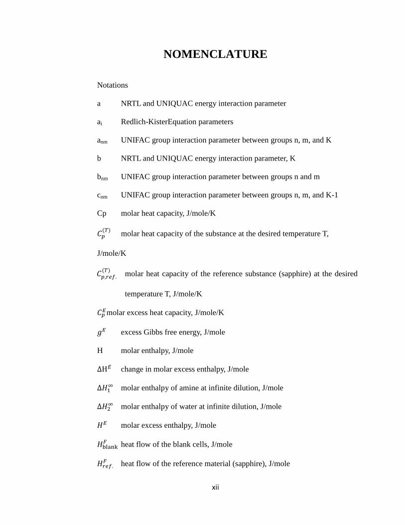
NOMENCLATURE

Notations

a NRTL and UNIQUAC energy interaction parameter

ai Redlich-KisterEquation parameters

anm UNIFAC group interaction parameter between groups n, m, and K

b NRTL and UNIQUAC energy interaction parameter, K

bnm UNIFAC group interaction parameter between groups n and m

cnm UNIFAC group interaction parameter between groups n, m, and K-1

Cp molar heat capacity, J/mole/K

molar heat capacity of the substance at the desired temperature T,

J/mole/K

molar heat capacity of the reference substance (sapphire) at the desired

temperature T, J/mole/K

molar excess heat capacity, J/mole/K

excess Gibbs free energy, J/mole

H molar enthalpy, J/mole

change in molar excess enthalpy, J/mole

molar enthalpy of amine at infinite dilution, J/mole

molar enthalpy of water at infinite dilution, J/mole

molar excess enthalpy, J/mole

heat flow of the blank cells, J/mole

heat flow of the reference material (sapphire), J/mole

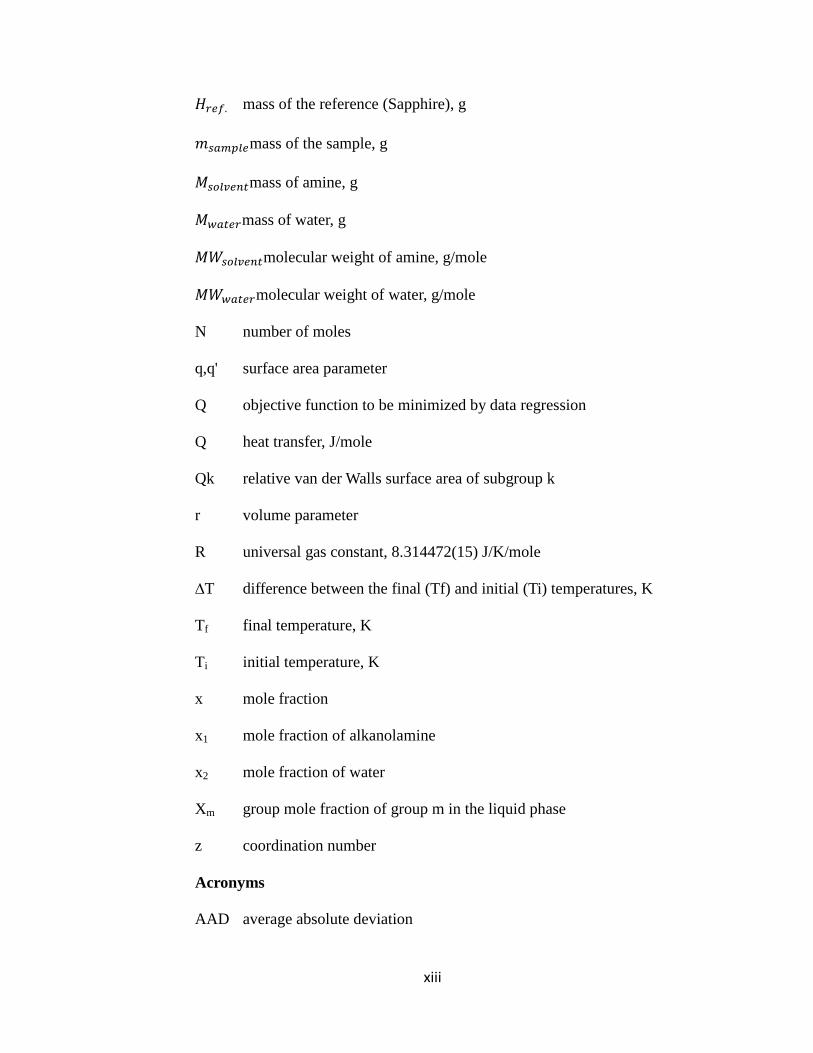
xiii

mass of the reference (Sapphire), g

mass of the sample, g

mass of amine, g

mass of water, g

molecular weight of amine, g/mole

molecular weight of water, g/mole

N number of moles

q,q' surface area parameter

Q objective function to be minimized by data regression

Q heat transfer, J/mole

Qk relative van der Walls surface area of subgroup k

r volume parameter

R universal gas constant, 8.314472(15) J/K/mole

∆T difference between the final (Tf) and initial (Ti) temperatures, K

Tf final temperature, K

Ti initial temperature, K

x mole fraction

x1 mole fraction of alkanolamine

x2 mole fraction of water

Xm group mole fraction of group m in the liquid phase

z coordination number

Acronyms

AAD average absolute deviation

xiv

MEA monoethanolamine

MDEA methyldiethanolamine

NRTL non-random two liquid

UNIFA universal quasi chemical functional group activity coefficients

Greek Letters

α randomness factor in NRTL model

group activity coefficient of group k in the mixture

group activity coefficient of group k in the pure substance

activity coefficient

θ area fraction in UNIQUAC model

surface fraction of group m in the liquid phase

number of structural groups of type k in molecule i

standard deviation of the indicated datainEquation

standard deviation

energy interaction perameters in NRTL and UNIQUAC models

segment fraction in UNIQUAC model

segment fraction in UNIQUAC model

Superscripts

c combinatorial

cal calculated value

e excess property

xv

exp experimental value

r residual

Subscripts

1 amine

12 interactions between amine and water

2 water

21 interactions between water and amine

i number of variables

i and j species

i,j interactions between I and j component

j numberof data points

j,i interactions between j and i component

k number of sets

m measured data

nm groups n and m

1

CHAPTER 1: INTRODUCTION

A greenhouse gas is a gas in the atmosphere that absorbs and emits radiation

within the thermal infrared range. Carbon dioxide (CO2), methane (CH4), nitrous oxide

(N2O), hydro-fluorocarbons (PFCs), cholorofluorocarbons (CFCs) and sulphur

hexafluoride (SF6) are major greenhouse gases and their contribution to the overall

greenhouse effect is based upon their emission volume, as well as their individual

greenhouse potentials. For instance, a methane molecule has 21 times the impact of one

molecule of CO2, nitrogen has 310 times, ground level ozone has 2000 times and CFC

has 13,000 to 20,000 times the impact of one molecules of CO2. However, CO2 is

considered the most influential Greenhouse gas (GHG) due to its large volume of

emission (6.0x109-8.2x10

9tonnes CO2/year on a dry air basis) into the atmosphere

(Henni, 2002).

Figure (1-1) Greenhouse Effect (Adopted from http:// www.ucar.edu)

2

Efforts to reduce the overall greenhouse gas (GHG) emissions began in the 1970s

(UNFCCC, 2007). Global CO2 emissions have increased by over 70% between 1971 and

2002. It is speculated that by the end of the century the earth’s average temperature

would increase by 1.4 to 6oC as carbon emissions reach approximately 26 Gt/year by the

year 2100. The effects of global warming have been felt inmany parts of world due to a

rise in sea levels, intense floods and climate change (Henni, 2002). In December 1997,

during the United Nations Framework Convention on Climate Change (UNFCCC), an

agreement was made between countries endorsing the treaty, to reduce global greenhouse

gas emissions by 2008-2012 at least 5% below the 1990 levels. Canada has agreed to

reduce its GHG emissions to 6% below 1990 levels. GHG emission control is best

implemented by projects like CCS (Carbon Dioxide Capture and Sequestration) in order

to reduce the concentration of CO2 in the atmosphere by reducing its emissions from

power plants and other large industrial sources. The goal of a CCS project is to develop

new technologies to capture CO2 from industrial gases and store it in deep geological

storage reservoirs, or for use in enhanced oil recovery (EOR).

To this end, CO2 capture technologywhich reducesgreenhouse gas emissions by

producing a stream of CO2that is transported to a storage site considered as one of the

most promising approaches that can be applied to power plants and large industrial

sectors asmajor sources of greenhouse gas emissions. The energy needed to operate CO2

capture units, however,requires some fuel consumption, reducesthe operational

efficiency, and may also have an impact on the environment. In spite of these drawbacks,

as more efficient capture methods become available, this technology will become more

competitive with lower emissions from fossil fuel. Optimization of required energy for

3

CO2 capture processes is important to make this technology cost-effective andhaveless

adverse impacts on the environment (Bet Metz et al., 2005).

The CO2 absorption process using aqueous alkanolamines is one of the most

promising methods for the removal of acid gas in industrial sectors. This process is based

on using alkanolamines as absorbents to remove CO2 from flue gas. The solvent

stripping process involves chemical reactions betweenthe solvent and CO2. Heating is

used toseparate the CO2 fromthe alkanolamine solution, which is regenerated in order to

be reused in the process. A drawback of the process is the limited lifetime of the amine

solution which becomes degraded due to oxidation and the high temperature of

regeneration. In addition,the occurrence of corrosionin the processneeds to be considered

(Leeet al., 2005). Currently, more energy-efficient solvents which possess suitable

physical and chemical properties need to be investigated. In this regard, knowledge of

the thermodynamic properties of new solvents, such as their heat of capacity and

enthalpies, is vital.

Molar heat capacity (Cp) is associated with basic thermodynamic properties such

as enthalpy, entropy and Gibbs energy. Knowledge of molar heat capacity is required to

evaluate the effect of temperature on chemical reactions (Czichos et al., 2006) and to

calculate the heat duty of equipment such as reboilers, heat exchangers and condensers in

gas-treating processes (Sandler et al., 2006).

Molar excess enthalpy (HE) is another significant thermodynamic property that

supplies information about the macroscopic behavior and molecular interactions between

the solvents in the solutions. Multistage and multi-component modeling of the CO2

absorption process also needs molar enthalpy data, and HE

values are required to develop

new theories (Sandler et al., 2006).

4

Figure (1-2) Process flow diagram for CO2 recovery from flue gas by amine absorption

5

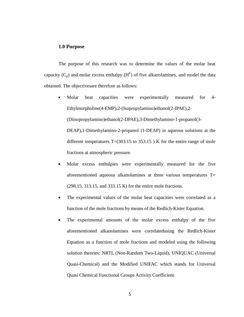
1.0 Purpose

The purpose of this research was to determine the values of the molar heat

capacity (Cp) and molar excess enthalpy (HE) of five alkanolamines, and model the data

obtained. The objectivesare therefore as follows:

Molar heat capacities were experimentally measured for 4-

Ethylmorpholine(4-EMP),2-(Isopropylamino)ethanol(2-IPAE),2-

(Diisopropylamino)ethanol(2-DPAE),3-Dimethylamino-1-propanol(3-

DEAP),1-Dimethylamino-2-propanol (1-DEAP) in aqueous solutions at the

different temperatures T=(303.15 to 353.15 ) K for the entire range of mole

fractions at atmospheric pressure.

Molar excess enthalpies were experimentally measured for the five

aforementioned aqueous alkanolamines at three various temperatures T=

(298.15, 313.15, and 333.15 K) for the entire mole fractions.

The experimental values of the molar heat capacities were correlated as a

function of the mole fractions by means of the Redlich-Kister Equation.

The experimental amounts of the molar excess enthalpy of the five

aforementioned alkanolamines were correlatedusing the Redlich-Kister

Equation as a function of mole fractions and modeled using the following

solution theories: NRTL (Non-Random Two-Liquid), UNIQUAC (Universal

Quasi-Chemical) and the Modified UNIFAC which stands for Universal

Quasi Chemical Functional Groups Activity Coefficient.

6

1.1 Scope

The five selected alkanolamines aqueous solutions were examined in terms of

molar heat capacity and molar excess enthalpy. Amongst the five chosen alkanolamines,

2-(Isopropylamino) ethanol (2-IPAE) is a secondary amine, 2-(Diisopropylamino)

ethanol (2-DPAE),3-Dimethylamino-1-propanol(3-DEAP), and 1-Dimethylamino-2-

propanol (1-DEAP) are tertiary amines and 4-Ethylmorpholine belongs to the cyclic

group of amine. There was no available data in the literature for the above-mentioned

alkanolamines aqueous solutions related to molar heat capacity and molar excess

enthalpy.

1.1.14-Ethylmorpholine

4-Ethylmorpholine is a colourless liquid with an ammonia-like odour. It is

flammable and a dangerous fire hazard. 4-Ethylmorpholine is used as a catalyst in the

manufacture of urethane foam, as an intermediate for dyestuffs, pharmaceuticals, rubber

accelerators and emulsifying agents, as a solvent for dyes, resins, oils, and as a substrate

for enzyme reactions (Health Council of the Netherlands).

1.1.22-(Isopropylamino)ethanol

2-(Isopropylamino)ethanol is highly flammable, with a boiling point of445K, and

it is slightly soluble in water. This amine is an aminoalcohol and chemical bases. It

neutralizes acids to form salts plus water. These acid-base reactions are exothermic. The

amount of heat that is evolved per mole of amine in neutralization is largely independent

7

of the strength of the amine as a base.

1.1.32-(Diisopropylamino)ethanol

2-(Diisopropylamino) ethanol is highly flammable, the range of boiling point

460-465Kand it is slightly soluble in water. This amine is an aminoalcohol and chemical

bases. It neutralizes acids to form salts plus water. These acid-base reactions are

exothermic. The amount of heat that is evolved per mole of amine in neutralization is

largely independent of the strength of the amine as a base.

1.1.43-Dimethylamino-1-propanol

3-Dimethylamino-1-propanol is a colourless to yellow liquid. The range of

boiling point is433-437K, and its melting point is238 K. It is stable, flammable and

incompatible with strong oxidizing agents.

1.1.51-Dimethylamino-2-propanol

1-Dimethylamino-2-propanol is a light yellow liquid. The range of its boiling

point is395-399 K, and its melting point is188 K. It is stable, flammable, and

incompatible with strong oxidizing agents, amines, and acids.

8

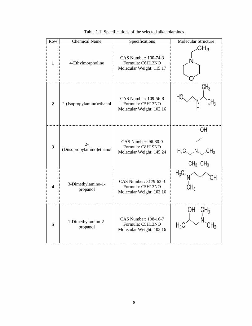
Table 1.1. Specifications of the selected alkanolamines

Row Chemical Name Specifications Molecular Structure

1 4-Ethylmorpholine

CAS Number: 100-74-3

Formula: C6H13NO

Molecular Weight: 115.17

2 2-(Isopropylamino)ethanol

CAS Number: 109-56-8

Formula: C5H13NO

Molecular Weight: 103.16

3 2-

(Diisopropylamino)ethanol

CAS Number: 96-80-0

Formula: C8H19NO

Molecular Weight: 145.24

4 3-Dimethylamino-1-

propanol

CAS Number: 3179-63-3

Formula: C5H13NO

Molecular Weight: 103.16

5 1-Dimethylamino-2-

propanol

CAS Number: 108-16-7

Formula: C5H13NO

Molecular Weight: 103.16

9

CHAPTER 2:LITERATURE REVIEW

The measurement of heat is associated with the exchange of heat. The exchange

of heat causes a temperature change in a substance and creates a heat flow leading to

temperature differences along its path which serves as a measurement of the flowing heat

(Perry et al., 2008). A calorimeter is a device used to measure the occurrence of a

chemical or physical process through measurement ofthe amount of the heat flow to or

from the system in order to attain the thermodynamic properties. Since the calorimeter

device is perfectly insulated and there is no heat exchange with its surroundings, the

device is able to measure the precise amount of heat absorbed or released during the

process.This measurement process is called calorimetry. Moreover, the calorimeter is

utilized to quantify the rates of heat flow as well as the characteristic temperatures of a

reaction.

The amount of heat transferred is related to the amount of change in the

temperature of a substance, and the relationship is as follows:

. is the amount of heat transferred, represents the heat capacity of the substance

defined as the amount of heat required to change the temperature of the given substance

by one degree, and represents the differentiation between the final and initial

temperatures denoted by respectively.

The values of enthalpy are utilized to determine the amount of heat duty in

different mixing or separation processes, and as a result, the enthalpy of formed-solution

changes per mole fraction because of the occurrence of the mixing process in the pure

components. Consequently the calorimetrically measurement values are referred to as the

10

molar excess enthalpy .

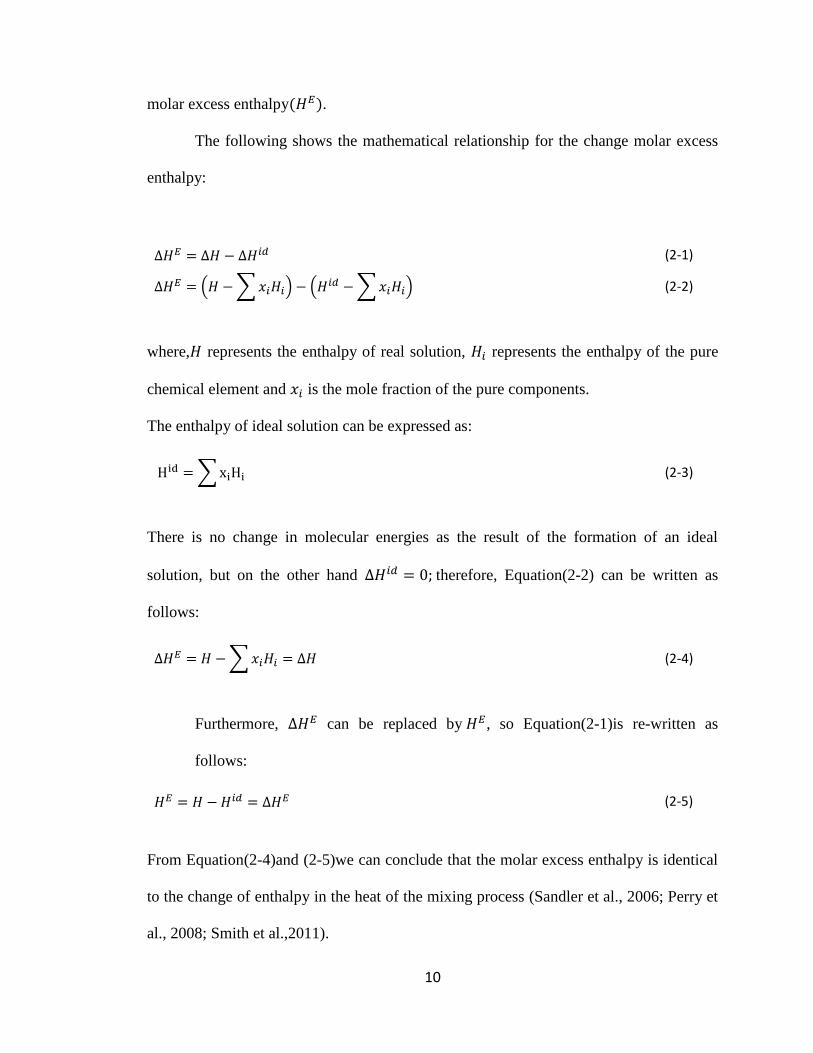
The following shows the mathematical relationship for the change molar excess

enthalpy:

(2-1)

(2-2)

where, represents the enthalpy of real solution, represents the enthalpy of the pure

chemical element and is the mole fraction of the pure components.

The enthalpy of ideal solution can be expressed as:

(2-3)

There is no change in molecular energies as the result of the formation of an ideal

solution, but on the other hand therefore, Equation (2-2) can be written as

follows:

(2-4)

Furthermore, can be replaced by , so Equation (2-1)is re-written as

follows:

(2-5)

From Equation (2-4)and (2-5)we can conclude that the molar excess enthalpy is identical

to the change of enthalpy in the heat of the mixing process (Sandler et al., 2006; Perry et

al., 2008; Smith et al.,2011).

11

2.1. Calorimeter Methods

2.1.1. Adiabatic Calorimeter

Adiabatic calorimetry deals with the quantification of energy liberated from a

reaction under adiabatic conditions.An adiabatic calorimeter is utilized when

experiments need to be run under low heat loss. In an adiabatic calorimeter, an insulator

is used to divide the two walls in order to keep the heat produced inside the calorimeter

which causes a rise in temperature.

Methods for adiabatic calorimetry consist of two categories: pressure resistance

or pressure compensated adiabatic calorimetry. The problem with this method is to have

relatively high thermal inertia and the temperature should not remain constant during the

run (Goodwin et al., 2003).

2.1.2. Isothermal Calorimeter

An isothermal calorimeter works based on the temperature dissimilarity between

the sample and its environment. The temperature must remain constant during the run.

An isothermal calorimeter is able to generate meticulous results and is utilized for

measuring molar excess enthalpy. In an isothermal calorimeter, neither corrections nor

compensation is required for the difference in heat content and heat loss, which can be

considered as advantages of this type of calorimeter. However, the measurements can

only be performed under phase change circumstances, which is the disadvantage of this

kind of calorimeter (Alonso et al.; Lim et al., 1994).

12

2.1.3. Isothermal Dilution Calorimeter

An isothermal dilution calorimeter is another isothermal method to measure the

molar excess enthalpy. In an isothermal dilution calorimeter, in order to maintain

isothermal conditions, energy in the form of electricity is utilized. In this method, an

element is added to a stirred vessel where the first component already exists. Once the

composition has reached the desired value, the injection of the second component may

be stopped. The value of heat of mixing is determined from the amount of the firstand

second components, as well as the amount of electrical energy, which are used to keep

the isothermal conditions (McGlashan et al., 1973).

2.1.4 Flow Calorimeter

In a flow calorimeter, both components are injected into a mixing compartment

simultaneously at a certain rate. In a flow calorimeter, a broad range of temperatures and

pressure measurements can be carried out in a shorter time compared to other methods

which is considered an advantage of this method, and it is known as one of the best

options for measuring heat of mixing for the majority of liquids (McGlashan et al.,

1969).

Generally, selection of a calorimeter type, such as batch or flow, depends on the

research demands. In chemical reactions, bio-processes and processes that involve phase

change, it is advisable to use a batch type, but, for measurement of heat of mixing,it is

much better to use a flow calorimeter.

13

2.2. Predictions and Correlation Approaches

In order to maximize usage of experimental data and avoid time consuming

processes and the difficulties involved in experimental measurements with the extra

elements of a multi-component process, it is suitable to use correlation and prediction

approaches. The following approaches are used in this research to predict and correlate

the properties of multi-component systems (Weidlich et al., 1987).

2.2.1. Experimental Expressions

2.2.1.1 Molar Excess Heat Capacity

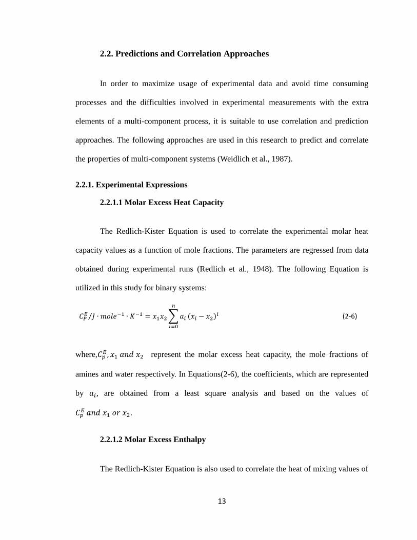
The Redlich-Kister Equation is used to correlate the experimental molar heat

capacity values as a function of mole fractions. The parameters are regressed from data

obtained during experimental runs (Redlich et al., 1948). The following Equation is

utilized in this study for binary systems:

(2-6)

where, represent the molar excess heat capacity, the mole fractions of

amines and water respectively. In Equations (2-6), the coefficients, which are represented

by , are obtained from a least square analysis and based on the values of

.

2.2.1.2 Molar Excess Enthalpy

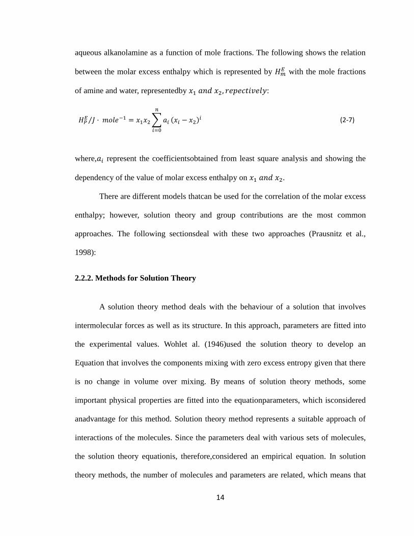
The Redlich-Kister Equation is also used to correlate the heat of mixing values of

14

aqueous alkanolamine as a function of mole fractions. The following shows the relation

between the molar excess enthalpy which is represented by with the mole fractions

of amine and water, representedby :

(2-7)

where, represent the coefficientsobtained from least square analysis and showing the

dependency of the value of molar excess enthalpy on .

There are different models thatcan be used for the correlation of the molar excess

enthalpy; however, solution theory and group contributions are the most common

approaches. The following sectionsdeal with these two approaches (Prausnitz et al.,

1998):

2.2.2. Methods for Solution Theory

A solution theory method deals with the behaviour of a solution that involves

intermolecular forces as well as its structure. In this approach, parameters are fitted into

the experimental values. Wohlet al. (1946)used the solution theory to develop an

Equation that involves the components mixing with zero excess entropy given that there

is no change in volume over mixing. By means of solution theory methods, some

important physical properties are fitted into the equationparameters, which isconsidered

anadvantage for this method. Solution theory method represents a suitable approach of

interactions of the molecules. Since the parameters deal with various sets of molecules,

the solution theory equationis, therefore,considered an empirical equation. In solution

theory methods, the number of molecules and parameters are related, which means that

15

greater numbers of molecules in a group needs more parameters (Whol et al., 1946).

In 1964, a new equationwas developed by Wilson. In his new proposal, the local

compositions were used instead of the mole fractions. With the equal number of

parameters this new Equationbetter represented the non-ideal behaviour of systems

compared to Wohl’sEquation. The other advantage of Wilson’s Equation was to represent

multi-component characterization with binary parameters; however, his Equation was not

able to cope with two liquid immiscibility conditions, which is considered themain

drawback of Wilson’s Equation.

A few years later, a model was developed by Prausnitz and his students based on

liquid-liquid theory which was called the NRTL (Prausnitz et al., 1968).The Non-

Random Two-Liquid, or NRTL,assumed that the liquid in the system is a binary

consisting of 2 types of molecules arranged in such a way that each of them is

surrounded by similar molecules and each individual surrounding molecule is encircled

in the same manner. The similarity between the NRTL model and Wilson Equation is

their accuracies in terms of correlation and prediction; however, the NRTL model can be

utilized for two liquid immiscible systems. One of the requirements in order to use the

NRTL model is to have three parameters for each pair of components, which is

considered a disadvantage of this model compared to the Wilson Equation. Cruz and his

co-worker later improved the NRTL model by extending it to the electrolyte solutions.

They combined the NRTL model with associated solution models,which resulted in

asatisfactory outcome in modeling molar excess enthalpies of alcohol solutions (Nagata

et al., 1984 and 1985).

UNIQUAC which stands for UNiversalQUAsi-Chemical Equation was

developed in 1975.Abrams and his colleague used concepts of both previous methods to

16

develop the UNIQUAC. In the universal quasi-chemical Equation, the activity

coefficients consist of two portions, the combinatorial and residual parts. The first part is

owing to different sizes and shapes of the molecules and the residual portion is because

of energetic interactions. Abrams and Prausnitz also demonstrated that by setting specific

parameters the Wohl and Wilson Equation as well as NRTL model could be considered

as special cases of the UNIQUAC model (Abramsand Prausnitz, 1975). Some features of

UNIQUAC Equation are as follows:

It can be applied to multi-components mixtures in relation to binary parameters

It can be applied to two-liquid equilibria

It can be used over moderate range is temperature dependency

It can represent mixtures of different molecular sizes

UNIQUAC involves complex algebraic parts, but despitethese complexities, sometimes

the result is not as accurate as the previous simpler methods, which is a drawback

ofUNIQUAC; however, the UNIQUAC Equation has room to be improved and is

considered a promising approach.

2.2.3. Methods of Group Contribution

Group contribution method is an optimized method to represent the experimental

data based upon the group contribution concept. The assumption made in the group

contribution method is that a real solution consists of the element group of its

components. Wilson and his colleagues developed this method for the first time, and it is

called an analytical solution of groups, although the concept was proposed by Langmuir

before (Wilson et al., 1962). In 1984, Vera and his co-workers proposeda simplified

17

group method analysis, which was a modified version of the group contribution methods

(Vera et al., 1984).UNIversal Functional Activity Coefficient (UNIFAC) was based on

previously developed methods in 1975. In UNIFAC, interaction in functional groups is

more important than molecules, which makes this method represent a broad range of

experimental values with fewerparameters,and also makes UNIFAC able to predict the

behaviour of systems more accuratelyeven when data are not available.

DISpersiveQUAsi Chemical (DISQUAC) is a group contribution method

thatutilizes the structure-dependent interaction parameters. In the DISQUAC method,

dispersive interchange energy characterizes each contact which could be polar or non-

polar. The quasi-chemical interchange energy and two more parameters characterize the

polar contacts (Kehiaianet al., 1978).

Basic knowledge regarding group elements of every component is needed for all

group contribution models; nevertheless, the calculations are more time consuming. It is

advisable to use either the solution theory method or group contribution model in order

to deal with experimental molar excess enthalpy data (Marongiu et al., 1996; Fanni et al.,

1996).

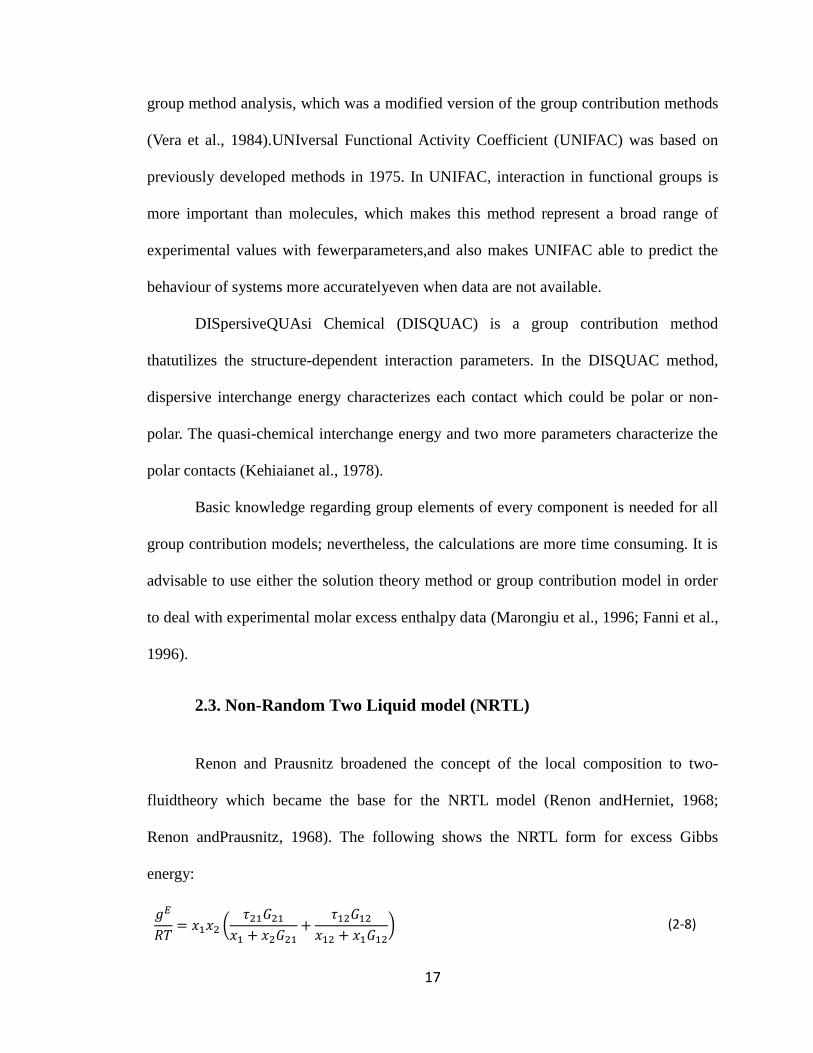
2.3. Non-Random Two Liquid model (NRTL)

Renon and Prausnitz broadened the concept of the local composition to two-

fluidtheory which became the base for the NRTL model (Renon andHerniet, 1968;

Renon andPrausnitz, 1968). The following shows the NRTL form for excess Gibbs

energy:

(2-8)

18

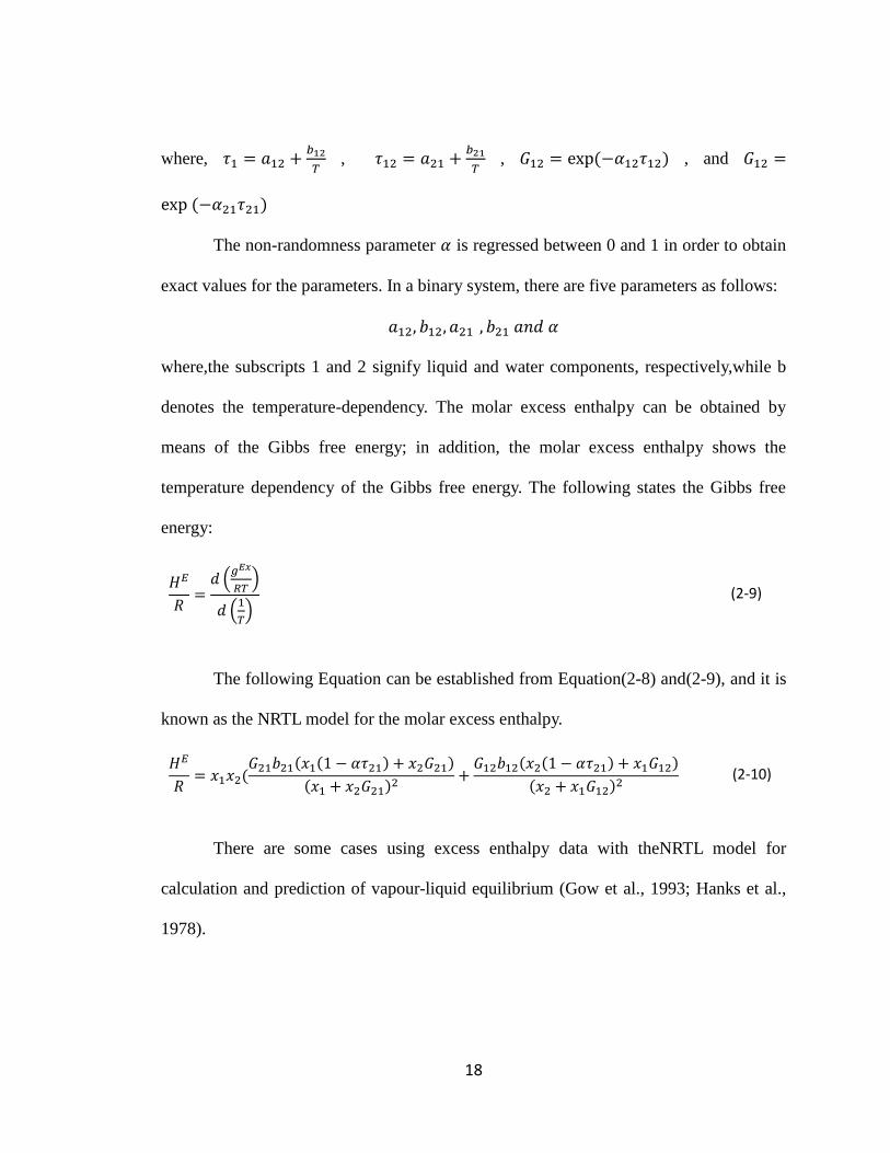
where,

,

, , and

The non-randomness parameter is regressed between 0 and 1 in order to obtain

exact values for the parameters. In a binary system, there are five parameters as follows:

where,the subscripts 1 and 2 signify liquid and water components, respectively,while b

denotes the temperature-dependency. The molar excess enthalpy can be obtained by

means of the Gibbs free energy; in addition, the molar excess enthalpy shows the

temperature dependency of the Gibbs free energy. The following states the Gibbs free

energy:

(2-9)

The following Equation can be established from Equation (2-8) and (2-9), and it is

known as the NRTL model for the molar excess enthalpy.

(2-10)

There are some cases using excess enthalpy data with theNRTL model for

calculation and prediction of vapour-liquid equilibrium (Gow et al., 1993; Hanks et al.,

1978).

19

2.4. Universal Quasi-Chemical Theory Model

Abrams and his co-worker found difficult inregressing data using the NRTL

model because of the lack of binary experimental data. They developed an Equation in

1975 based on the quasi-chemical theorydeveloped by Guggenheim. The Equation was

called the Universal Quasi-Chemical theory (UNIQUAC), which is an extension of the

above-mentioned theory for non-random mixtures (Abrams et al., 1975).

Combinatorial and residualare the two main portions in UNIQUAC model. The

residual part deals with the inter-molecular forces, which are obtained from the energy of

interactions and the mole fractions while the combinatorial part is involved in

combinatorial effects because of dissimilarity in size and shape of molecules.

Combinatorial parts consist of the segment fraction and the mole fraction. By

using the pure-components molecular structure, the amounts for the fractions can be

obtained; however, the pure-components molecular structure depends on the size of the

molecular and outer surface area. Since no adjustment binary parameters come into

existence in the combinatorial part,the correlations for experimental data are not

necessary to obtain contribution of the combinatorial part.

The energy interactions are represented by two parameters, and these parameters

cannot be measured; therefore, the best way to determine them is to regress these data

from two-liquid or vapour-liquid equilibrium.

The following represents UNIQUAC Equation:

(2-11)

The following formula shows a binary mixture:

20

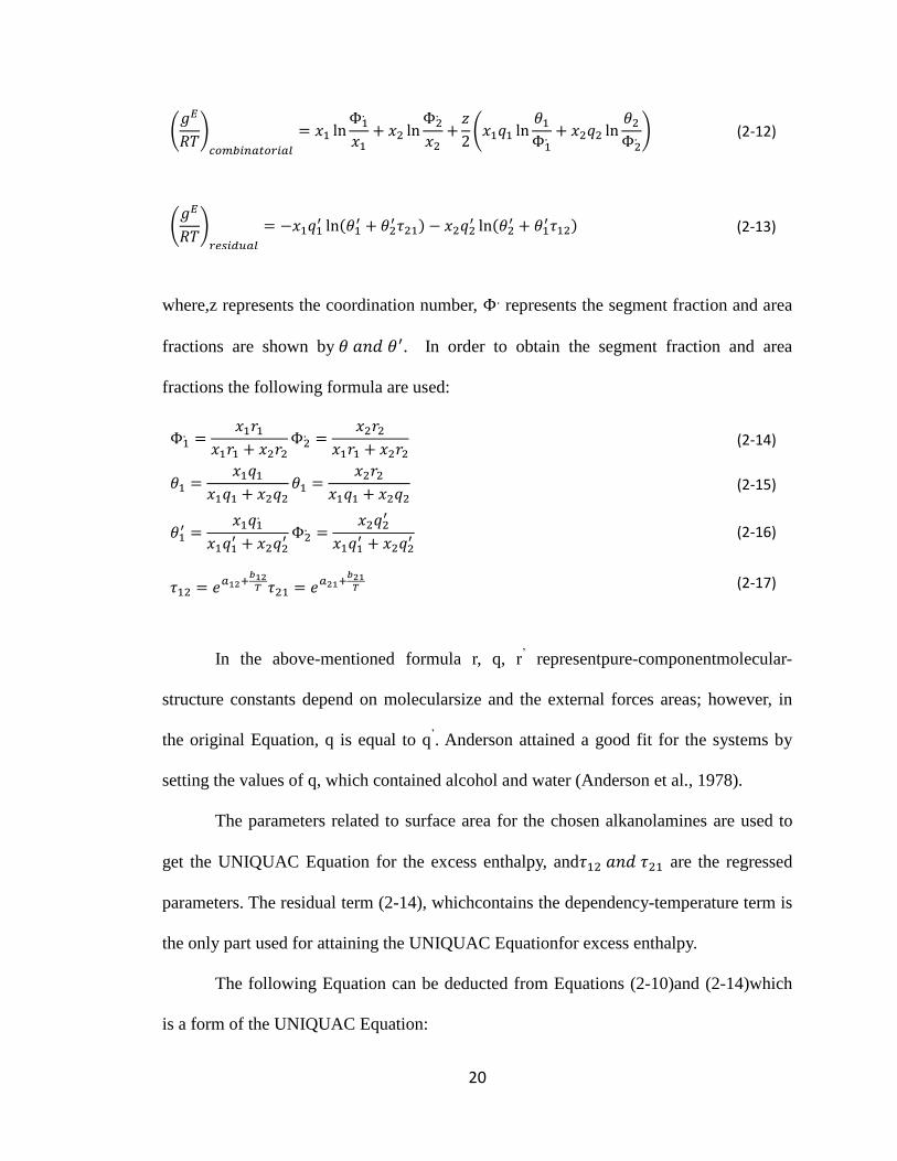
(2-12)

(2-13)

where,z represents the coordination number, represents the segment fraction and area

fractions are shown by . In order to obtain the segment fraction and area

fractions the following formula are used:

(2-14)

(2-15)

(2-16)

(2-17)

In the above-mentioned formula r, q, r’ representpure-componentmolecular-

structure constants depend on molecularsize and the external forces areas; however, in

the original Equation, q is equal to q’. Anderson attained a good fit for the systems by

setting the values of q, which contained alcohol and water (Anderson et al., 1978).

The parameters related to surface area for the chosen alkanolamines are used to

get the UNIQUAC Equation for the excess enthalpy, and are the regressed

parameters. The residual term (2-14), whichcontains the dependency-temperature term is

the only part used for attaining the UNIQUAC Equationfor excess enthalpy.

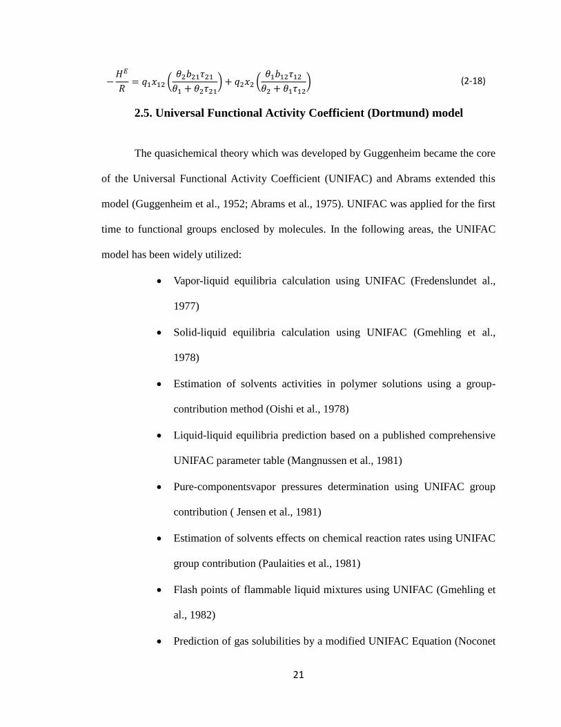
The following Equation can be deducted from Equations (2-10)and (2-14)which

is a form of the UNIQUAC Equation:

21

(2-18)

2.5. Universal Functional Activity Coefficient (Dortmund) model

The quasichemical theory which was developed by Guggenheim became the core

of the Universal Functional Activity Coefficient (UNIFAC) and Abrams extended this

model (Guggenheim et al., 1952; Abrams et al., 1975). UNIFAC was applied for the first

time to functional groups enclosed by molecules. In the following areas, the UNIFAC

model has been widely utilized:

Vapor-liquid equilibria calculation using UNIFAC (Fredenslundet al.,

1977)

Solid-liquid equilibria calculation using UNIFAC (Gmehling et al.,

1978)

Estimation of solvents activities in polymer solutions using a group-

contribution method (Oishi et al., 1978)

Liquid-liquid equilibria prediction based on a published comprehensive

UNIFAC parameter table (Mangnussen et al., 1981)

Pure-componentsvapor pressures determination using UNIFAC group

contribution ( Jensen et al., 1981)

Estimation of solvents effects on chemical reaction rates using UNIFAC

group contribution (Paulaities et al., 1981)

Flash points of flammable liquid mixtures using UNIFAC (Gmehling et

al., 1982)

Prediction of gas solubilities by a modified UNIFAC Equation (Noconet

22

al., 1983)

Some drawbacks were found in using the UNIFAC model, such as inadequate

results for the calculation of the activity coefficients at infinite dilution as mentioned by

Wieldlich et al., in 1987, especially for systems that involve molecules with various

sizes. Another disadvantage of UNIFAC is that the model is neither capable of accurate

predictions of the excess enthalpy nor the temperature-dependency of the Gibbs

Equation. Due to these drawbacks,Wieldlich decided to alter the genuine UNIFAC model

by setting one parameter that could precisely measure the heat of mixing and activity

coefficient at infinite dilution; however the description of the original UNIFAC Equation

was provided elsewhere (Fredenslund et al., 1977).

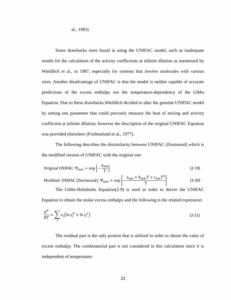
The following describes the dissimilarity between UNIFAC (Dortmund) which is

the modified version of UNIFAC with the original one:

(2-19)

(2-20)

The Gibbs-Helmholtz Equation (2-9) is used in order to derive the UNIFAC

Equation to obtain the molar excess enthalpy and the following is the related expression:

(2-21)

The residual part is the only portion that is utilized in order to obtain the value of

excess enthalpy. The combinatorial part is not considered in this calculation since it is

independent of temperature:

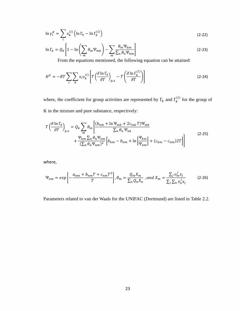
23

(2-22)

(2-23)

From the equations mentioned, the following equation can be attained:

(2-24)

where, the coefficient for group activities are represented by and

for the group of

K in the mixture and pure substance, respectively:

(2-25)

where,

(2-26)

Parameters related to van der Waals for the UNIFAC (Dortmund) are listed in Table 2.2.

24

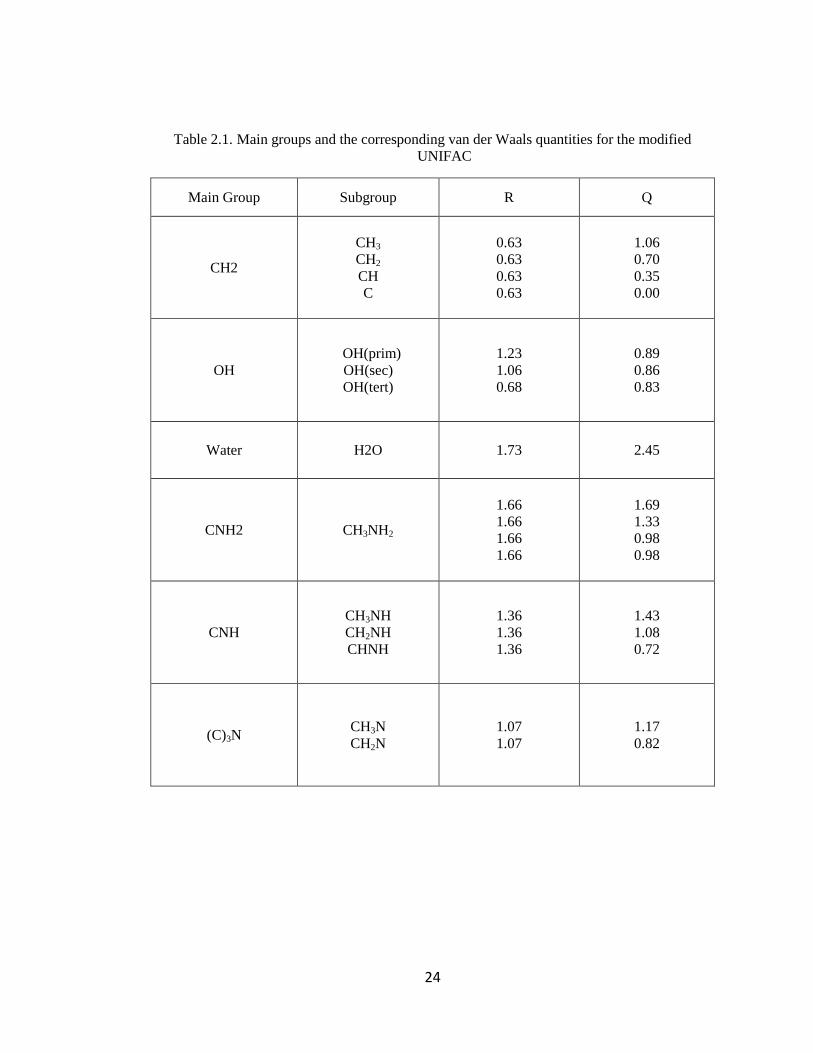
Table 2.1. Main groups and the corresponding van der Waals quantities for the modified

UNIFAC

Main Group Subgroup R Q

CH2

CH3

CH2

CH

C

0.63

0.63

0.63

0.63

1.06

0.70

0.35

0.00

OH

OH(prim)

OH(sec)

OH(tert)

1.23

1.06

0.68

0.89

0.86

0.83

Water H2O 1.73 2.45

CNH2 CH3NH2

1.66

1.66

1.66

1.66

1.69

1.33

0.98

0.98

CNH

CH3NH

CH2NH

CHNH

1.36

1.36

1.36

1.43

1.08

0.72

(C)3N CH3N

CH2N

1.07

1.07

1.17

0.82

25

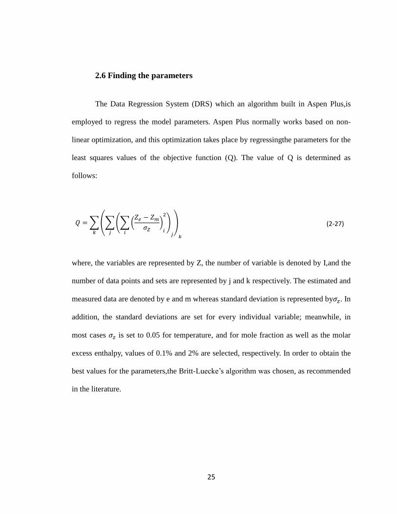
2.6 Finding the parameters

The Data Regression System (DRS) which an algorithm built in Aspen Plus,is

employed to regress the model parameters. Aspen Plus normally works based on non-

linear optimization, and this optimization takes place by regressingthe parameters for the

least squares values of the objective function (Q). The value of Q is determined as

follows:

(2-27)

where, the variables are represented by Z, the number of variable is denoted by I,and the

number of data points and sets are represented by j and k respectively. The estimated and

measured data are denoted by e and m whereas standard deviation is represented by . In

addition, the standard deviations are set for every individual variable; meanwhile, in

most cases is set to 0.05 for temperature, and for mole fraction as well as the molar

excess enthalpy, values of 0.1% and 2% are selected, respectively. In order to obtain the

best values for the parameters,the Britt-Luecke’s algorithm was chosen, as recommended

in the literature.

26

CHAPTER 3: EXPERIMENTAL METHODS

A heat flow calorimeter C-80, manufactured by Setaram Co.,was used in this

study to measure the experimental values for the molar heat capacity and molar excess

enthalpy. The description of the apparatus, procedure, calibration, and verifications are

discussed in this chapter. There are sources of error in the experiment which are included

and examined in Chapter 3, as well.

3.1. Equipment

A C80 Calvet Calorimeter is the instrument used in order to obtain experimental

values for the molar heat capacity and excess enthalpy. Setaram Instrumentation

Company from France manufactured the C80, and Tian-Calvet heat flow is employed as

the principletheory for this equipment. Calvet and his colleagues developed and

elaborated the Tian-Calvetmethod (Calvet et al., 1963).

There is data acquisition softwaretasked with obtaining and processing data from

C80,and it is compatible with Microsoft Windows. The temperature range in which C80

works is within 293 to 573 K. The sensitivity of the device is and the

measured and controlled pressure range is up to 1000 bar (Setaram).

The rate of heat flow measured by Calvet calorimeter is a function of

temperature. This rate has the same quantity of power that is needed to maintain the

sample temperature; however, it increases at a specific rate which is called the scanning

rate. The actual measurement is the deviation between the supplied power to the cells

27

and the calorimetric block. The signal measurement represents the power that is needed

by the sample heater in order to keep the sample and reference both in isothermal

condition. The measured signal considered as the heat of mixing or specific heat of the

sample.

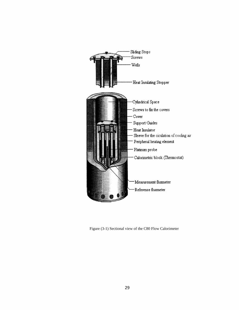
A C80 calorimeter generally consists of a chamber and a fluxmeter located at the

center of the chamber. There is an aluminum block that functions as a thermostat in the

calorimeter and is located at the center of the shell. The shell which looks like a

cylindrical is shown in Figure 3-1, together with other internal elements of the

calorimeter. In the C80, individual cells for the sample and reference are used and are

symmetrically placed into two similar cavities from the centerline of the shell. Standards

and membrane mixing are two types of sample cells used to measure the molar heat

capacity and excess enthalpy, respectively. Due to the instability of residual temperature,

there would be signal disturbances and to avoid these interfering signals, a separate

thermopile surrounds each cell, which is called a fluxmeter. These fluxmeters have the

same design and since they are linked in opposition they can provide a differential

output. Both cells are connected to the block through the fluxmeters. Each cell consists

of concentric rings and thermocouples. A detector is used in the C80 that takes

independent measurements in terms of the weights and shape of the sample (Setaram).

In order to measure and monitor the temperature of each cell, two platinum

probes are separately utilized. These two probes are placed inside the calorimeter and

denoted as PT1 and PT2. The temperature of the cells is measured by the first resistance

probe and this measurement takes place inside the calorimeter. The location of PT1 is

somewhere in between two cells. PT1 is linked to the safety unit for the temperature and

has resistance of 100 ohm at 273.15 K. The power is shut down automatically in case of

28

exceeding the maximum temperature. The other probe which is named, PT2, contributes

by controlling the block temperature and is connected to temperature controller unit. The

controller is assigned to maintain the experimental temperature of the C80 which is

already set, and it is linked to the aluminum heater block. For the purpose of thermal

insulation and cooling an air gap is set up adjacent to the insulating material that

surrounds the block.

29

Figure (3-1) Sectional view of the C80 Flow Calorimeter

30

3.2. Calibration

The C80 calorimeter needs to be calibrated in order to produce accurate output.

The calibration consists of two parts, the temperature scale and a sensitivity test.

Standard procedure aids in calibrating the C80 for both items. ICTAC, which is the

Confederation of National or Regional Thermal Analysis and Calorimetry Societies,

developed standards for the sensitivity and temperature calibration.

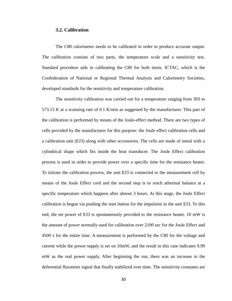
The sensitivity calibration was carried out for a temperature ranging from 303 to

573.15 K at a scanning rate of 0.1 K/min as suggested by the manufacturer. This part of

the calibration is performed by means of the Joule-effect method. There are two types of

cells provided by the manufacturer for this purpose: the Joule effect calibration cells and

a calibration unit (EJ3) along with other accessories. The cells are made of metal with a

cylindrical shape which fits inside the heat transducer. The Joule Effect calibration

process is used in order to provide power over a specific time for the resistance heater.

To initiate the calibration process, the unit EJ3 is connected to the measurement cell by

means of the Joule Effect cord and the second step is to reach athermal balance at a

specific temperature which happens after almost 3 hours. At this stage, the Joule Effect

calibration is begun via pushing the start button for the impulsion in the unit EJ3. To this

end, the set power of EJ3 is spontaneously provided to the resistance heater. 10 mW is

the amount of power normally used for calibration over 2100 sec for the Joule Effect and

4500 s for the entire time. A measurement is performed by the C80 for the voltage and

current while the power supply is set on 10mW, and the result in this case indicates 9.99

mW as the real power supply. After beginning the run, there was an increase in the

deferential fluxmeter signal that finally stabilized over time. The sensitivity constants are

31

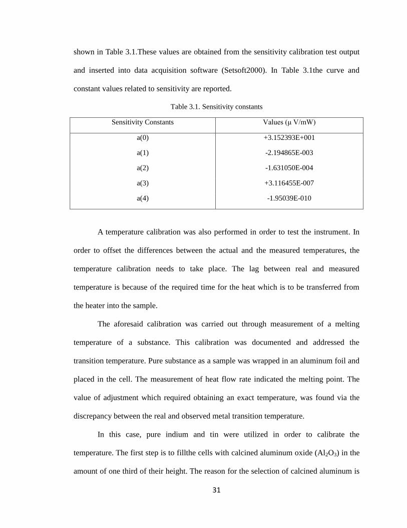
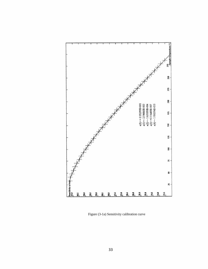
shown in Table 3.1.These values are obtained from the sensitivity calibration test output

and inserted into data acquisition software (Setsoft2000). In Table 3.1the curve and

constant values related to sensitivity are reported.

Table 3.1. Sensitivity constants

Sensitivity Constants Values (μ V/mW)

a(0) +3.152393E+001

a(1) -2.194865E-003

a(2) -1.631050E-004

a(3) +3.116455E-007

a(4) -1.95039E-010

A temperature calibration was also performed in order to test the instrument. In

order to offset the differences between the actual and the measured temperatures, the

temperature calibration needs to take place. The lag between real and measured

temperature is because of the required time for the heat which is to be transferred from

the heater into the sample.

The aforesaid calibration was carried out through measurement of a melting

temperature of a substance. This calibration was documented and addressed the

transition temperature. Pure substance as a sample was wrapped in an aluminum foil and

placed in the cell. The measurement of heat flow rate indicated the melting point. The

value of adjustment which required obtaining an exact temperature, was found via the

discrepancy between the real and observed metal transition temperature.

In this case, pure indium and tin were utilized in order to calibrate the

temperature. The first step is to fillthe cells with calcined aluminum oxide (Al2O3) in the

amount of one third of their height. The reason for the selection of calcined aluminum is

32

its properties regarding phase transition. Within the specific range of temperature used in

this study, Al2O3 has no phase transition and Al2O3 affects just the thermal mass in such

a way that it adds this mass to the cells, and consequently, the amount of the molar heat

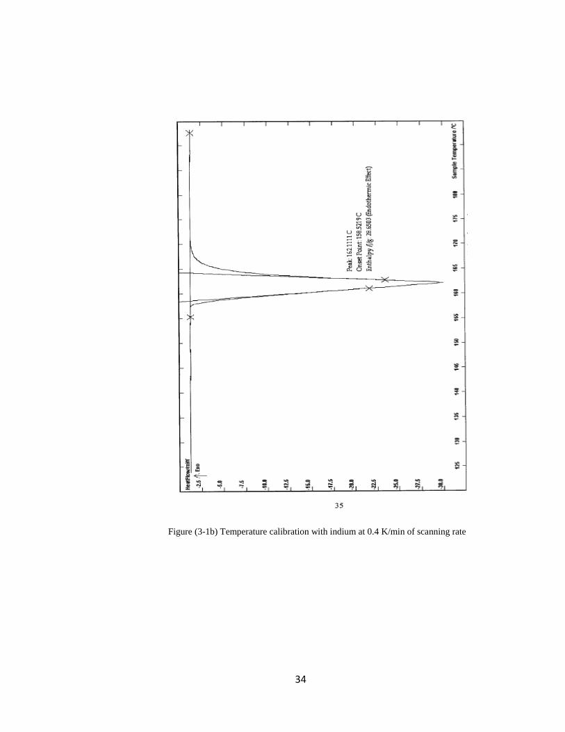
capacity is increased. As shown in Figure (3-1b),the measurement underneath the peak

area can be used to calculate the total heat amount thatwas absorbed by the sample over

the melting period. On the other hand, the melting point indicates the temperature

marking the beginning of the rise in heat flow in the melting process. This temperature is

considered as the alleged melting temperature if this is defined in terms of indicated

temperature over melting process in the calorimeter. The amount obtained via this

process is dependent on the rate of heating. The measurement takes place over different

rates of heating for both substances. In order to obtain the differences between the real

and observed temperature the software was utilized and theses values are denote by

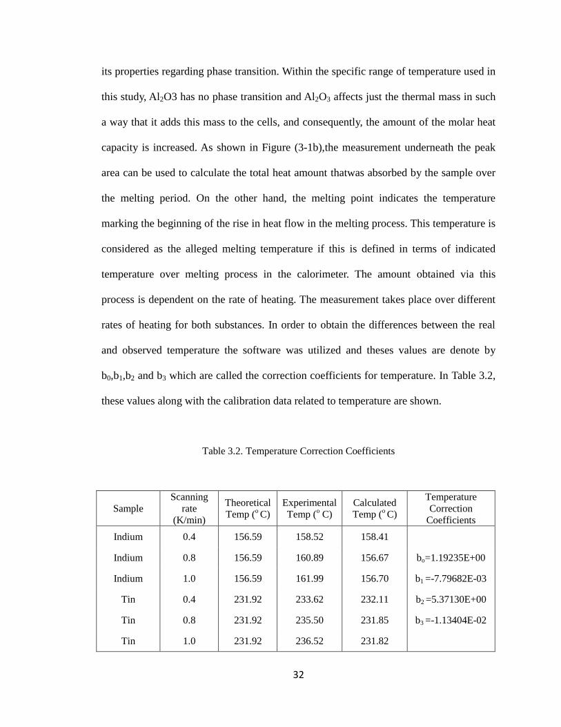
b0,b1,b2 and b3 which are called the correction coefficients for temperature. In Table 3.2,

these values along with the calibration data related to temperature are shown.

Table 3.2. Temperature Correction Coefficients

Sample

Scanning

rate

(K/min)

Theoretical

Temp (o C)

Experimental

Temp (o C)

Calculated

Temp (o C)

Temperature

Correction

Coefficients

Indium 0.4 156.59 158.52 158.41

Indium 0.8 156.59 160.89 156.67 bo=1.19235E+00

Indium 1.0 156.59 161.99 156.70 b1 =-7.79682E-03

Tin 0.4 231.92 233.62 232.11 b2 =5.37130E+00

Tin 0.8 231.92 235.50 231.85 b3 =-1.13404E-02

Tin 1.0 231.92 236.52 231.82

33

Figure (3-1a) Sensitivity calibration curve

34

Figure (3-1b) Temperature calibration with indium at 0.4 K/min of scanning rate

35

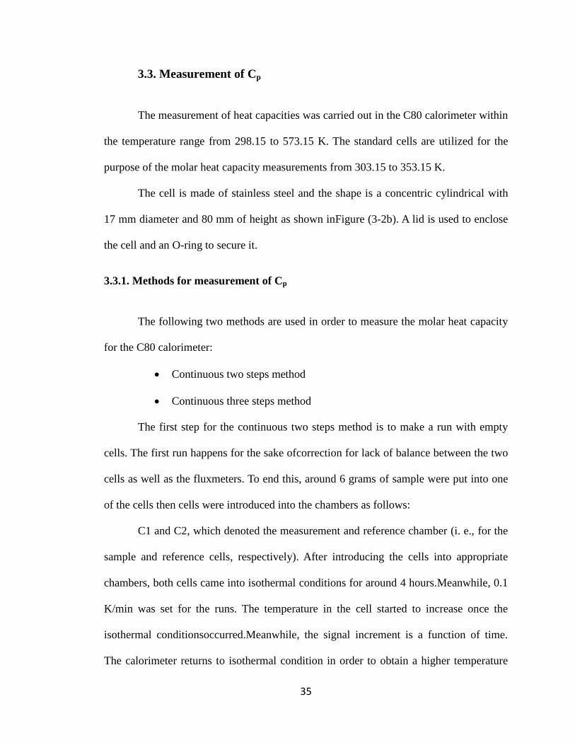
3.3. Measurement of Cp

The measurement of heat capacities was carried out in the C80 calorimeter within

the temperature range from 298.15 to 573.15 K. The standard cells are utilized for the

purpose of the molar heat capacity measurements from 303.15 to 353.15 K.

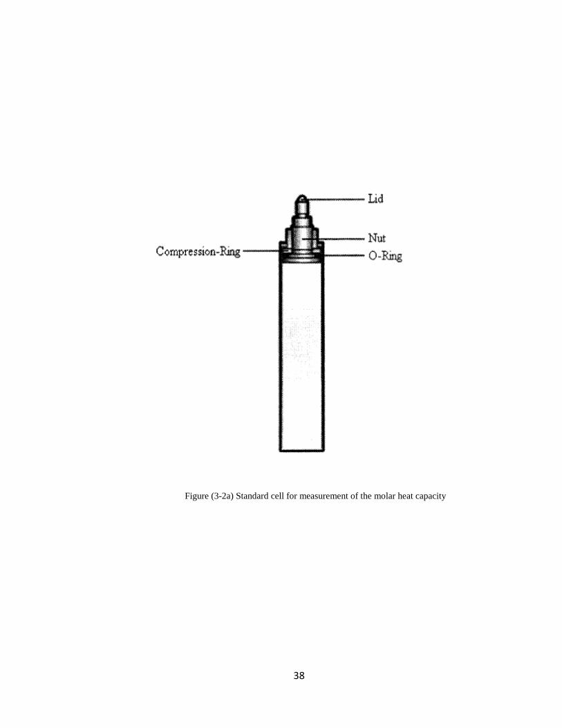
The cell is made of stainless steel and the shape is a concentric cylindrical with

17 mm diameter and 80 mm of height as shown inFigure (3-2b). A lid is used to enclose

the cell and an O-ring to secure it.

3.3.1. Methods for measurement of Cp

The following two methods are used in order to measure the molar heat capacity

for the C80 calorimeter:

Continuous two steps method

Continuous three steps method

The first step for the continuous two steps method is to make a run with empty

cells. The first run happens for the sake ofcorrection for lack of balance between the two

cells as well as the fluxmeters. To end this, around 6 grams of sample were put into one

of the cells then cells were introduced into the chambers as follows:

C1 and C2, which denoted the measurement and reference chamber (i. e., for the

sample and reference cells, respectively). After introducing the cells into appropriate

chambers, both cells came into isothermal conditions for around 4 hours.Meanwhile, 0.1

K/min was set for the runs. The temperature in the cell started to increase once the

isothermal conditionsoccurred.Meanwhile, the signal increment is a function of time.

The calorimeter returns to isothermal condition in order to obtain a higher temperature

36

which causes the signal of the calorimeter also to get back to the baseline.

The continuous steps method is meant for molar heat capacity measurements as

used by Becker et al. (2000) and Gmehling et al. (2001). They applied the aforesaid

method in order to measure the molar heat capacity for several organic substances. In the

three steps method, the scan rate is 0.1 K/min and there are three runs for this method

such as sample, blank and reference runs which is the only difference between the two

and three continuous steps method. The rest of the procedure is the same as in the

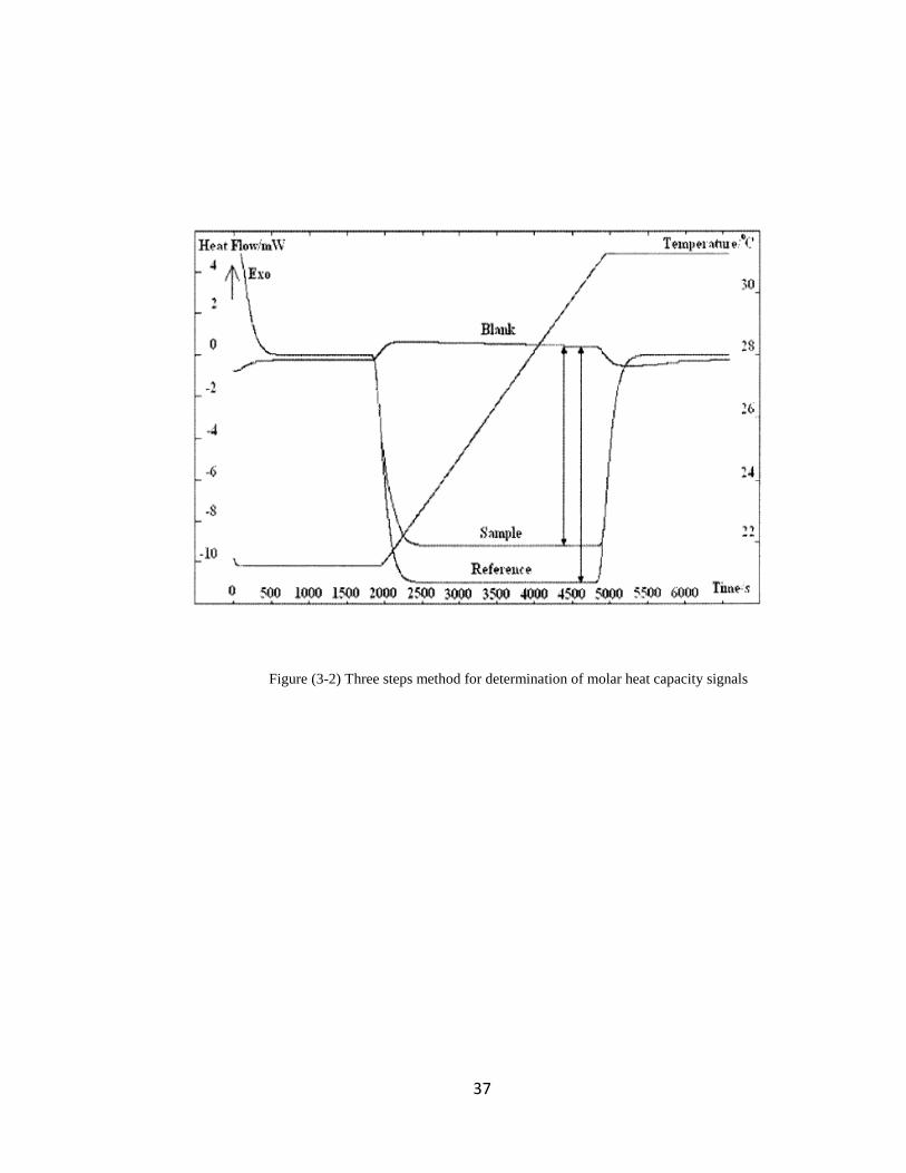
previous method. The condition of the experiments in three steps is the same. In 0Figure

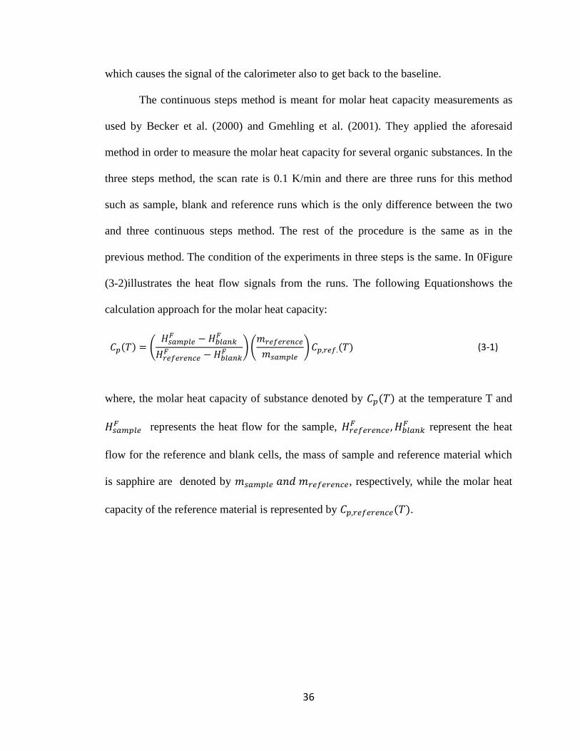
(3-2)illustrates the heat flow signals from the runs. The following Equationshows the

calculation approach for the molar heat capacity:

(3-1)

where, the molar heat capacity of substance denoted by at the temperature T and

represents the heat flow for the sample,

represent the heat

flow for the reference and blank cells, the mass of sample and reference material which

is sapphire are denoted by , respectively, while the molar heat

capacity of the reference material is represented by .

37

Figure (3-2) Three steps method for determination of molar heat capacity signals

38

Figure (3-2a) Standard cell for measurement of the molar heat capacity

39

3.4. Measurement of Heat of Mixing

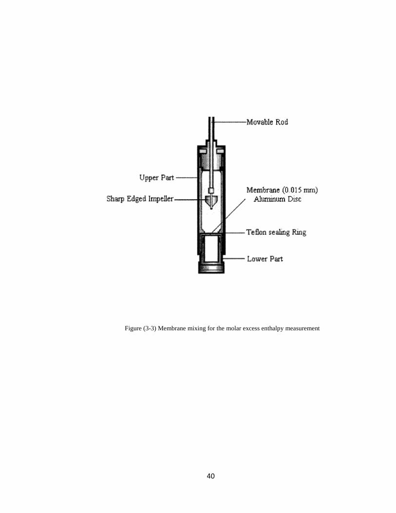
The C80 flow calorimeter alsohas the ability to measure the heat of mixing,

which is carried out in this study at three temperatures (298.15, 313.15 and 333.15 K).

For the purpose of the molar excess enthalpy measurement a membrane mixing cell is

utilized. Two membrane cells are needed: one is for measurement and the other is used

for the reference chamber. Amine and water are put into two compartments and separated

by means of a layer of aluminum foil. These two parts are mixed after enough time has

passed when the experiment is running. The reference cell is meant to maintain the

isothermal conditions by canceling the supplied heat as well as the small amount of heat

produced during the stirring process. After both cells are introduced into the calorimeter,

it is important to allow the calorimeter temperature to become stabilized before

initiatingthe stirring step. The stirring process is monitored through the heat flow display;

once it starts to decrease the stirring process has to be halted. The difference between the

cells and the calorimeter block in terms of the heat flow is considered as the measured

flux. In terms of receiving heat to the cells, the block has enough thermal mass. In Figure

(3-4) shows that the time against the heat flows produced a curve. The total amount of

molar excess enthalpy for the sample was calculated via an integration operation of the

area which was located underneath the curve.

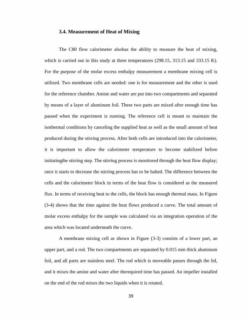
A membrane mixing cell as shown in Figure (3-3) consists of a lower part, an

upper part, and a rod. The two compartments are separated by 0.015 mm thick aluminum

foil, and all parts are stainless steel. The rod which is moveable passes through the lid,

and it mixes the amine and water after therequired time has passed. An impeller installed

on the end of the rod mixes the two liquids when it is rotated.

40

Figure (3-3) Membrane mixing for the molar excess enthalpy measurement

41

Figure (3-4) Molar excess enthalpy graph

42

3.5. Errors

The main errors, which may occur during the runs and preparation time of the

sample, occur of the following reasons:

Possible CO2 absorption from the air during sample preparation

The solvent does not mix well with water because a portion of the solvent

gets stuck to the cell wall

By avoiding the abovementioned source of error, the results of the experiments

can be made more accurate.

3.6. Preparation of solution

For the purpose of solution preparation an Ohaus analytical plus balance Model

AP250D ranging in 0.01mg resolution up to 52 g was utilized. The preparation is based

on the mole fraction and the following formula determines the required amount of water

for the solution:

(3-2)

where, the mole fraction of amines, mass of amines, and mass of water are denoted by

while represent the molecular weight of

alkanolamines and molecular weight of water respectively.

(3-3)

43

where, N represents the number of moles and is obtained as follows:

(3-4)

(3-5)

(3-6)

(3-7)

(3-8)

(3-9)

The amount of water for a particular mole fraction of solvent can be determined

by using Equation (3-9).

3.7. Verification of the C80 calorimeter

The C80 calorimeter has to be calibrated before use in order to determine the

accuracy of the equipment. To this end, two recognized amines,MDEA (99% mass

purity) and MEA (99% mass purity), were used for the purpose of testing the C80

calorimeter. Both were purchased from Sigma-Aldrich. The measurements of heat

capacities for both alkanolamines were carried out, and a comparison was made with the

available literature data within the temperature range from 303.15 to 353.15 K for the

entire mole fraction.

The measurement of heat of capacities using DSC wasdone by Chen et al. (2001)

44

and Chiu et al.(1999) for MDEA and MEA for temperatures from 303.15 to 353.15 K.

The scanning rate of 0.1 K/min was used for the measurement. The comparison with data

from literature shows absolute average deviations of 1.09% and 0.74% for MEA and

MDEA, respectively. The comparison is shown inFigures (3-5) and (3-6).

For the purpose of verification of the C80 heat flow calorimeter in terms of molar

excess enthalpy measurements, methyldiethanolamine and diethanolaminewere selected

as solvents as datafor their molar excess enthalpies were available in literature. The

corresponding data for the entire mole fractions at temperatures of 298.15, and 313.15 K

for DEA and MDEA respectively,were reported (Maham et al., 1997). Based on 2%

deviation for the measurement of the molar excess enthalpy for the entire mole fraction,

the measured values for calibration were in the acceptable range. The measured values

are listed in Table 3.4 and shown inFigure (3-6).

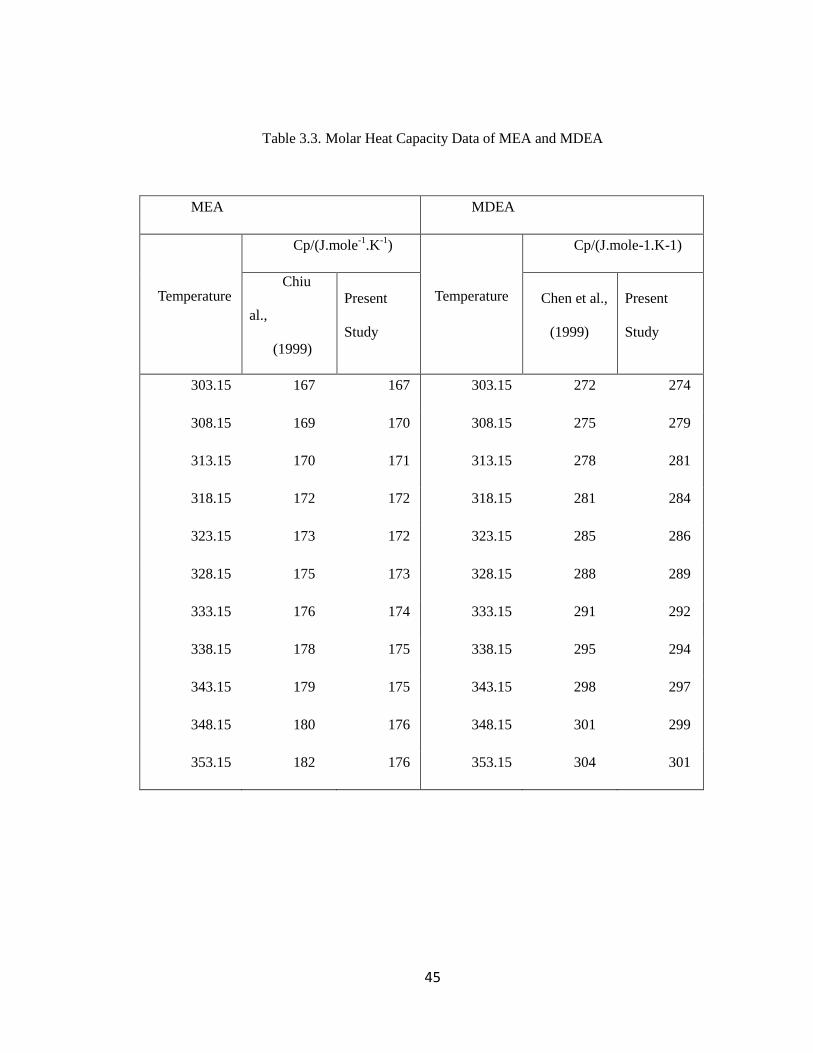
45

Table 3.3. Molar Heat Capacity Data of MEA and MDEA

MEA MDEA

Temperature

Cp/(J.mole-1

.K-1

)

Temperature

Cp/(J.mole-1.K-1)

Chiu

al.,

(1999)

Present

Study

Chen et al.,

(1999)

Present

Study

303.15 167 167 303.15 272 274

308.15 169 170 308.15 275 279

313.15 170 171 313.15 278 281

318.15 172 172 318.15 281 284

323.15 173 172 323.15 285 286

328.15 175 173 328.15 288 289

333.15 176 174 333.15 291 292

338.15 178 175 338.15 295 294

343.15 179 175 343.15 298 297

348.15 180 176 348.15 301 299

353.15 182 176 353.15 304 301

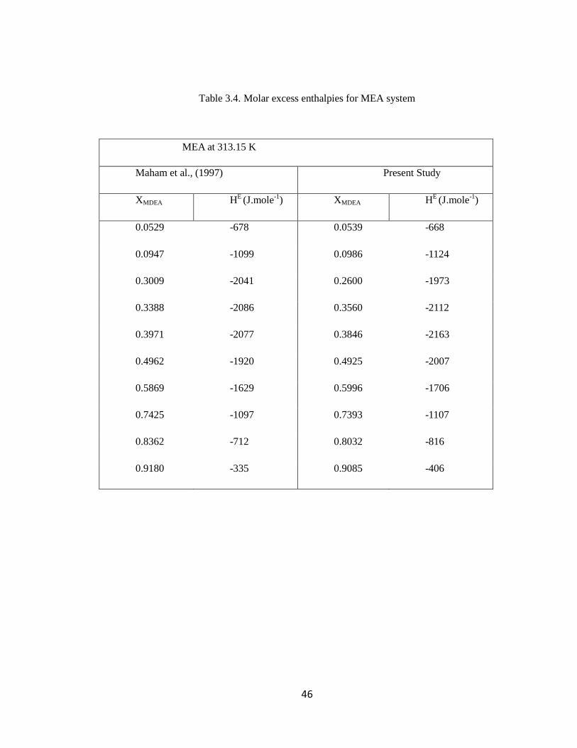
46

Table 3.4. Molar excess enthalpies for MEA system

MEA at 313.15 K

Maham et al., (1997) Present Study

XMDEA HE

(J.mole-1

) XMDEA HE

(J.mole-1

)

0.0529 -678 0.0539 -668

0.0947 -1099 0.0986 -1124

0.3009 -2041 0.2600 -1973

0.3388 -2086 0.3560 -2112

0.3971 -2077 0.3846 -2163

0.4962 -1920 0.4925 -2007

0.5869 -1629 0.5996 -1706

0.7425 -1097 0.7393 -1107

0.8362 -712 0.8032 -816

0.9180 -335 0.9085 -406

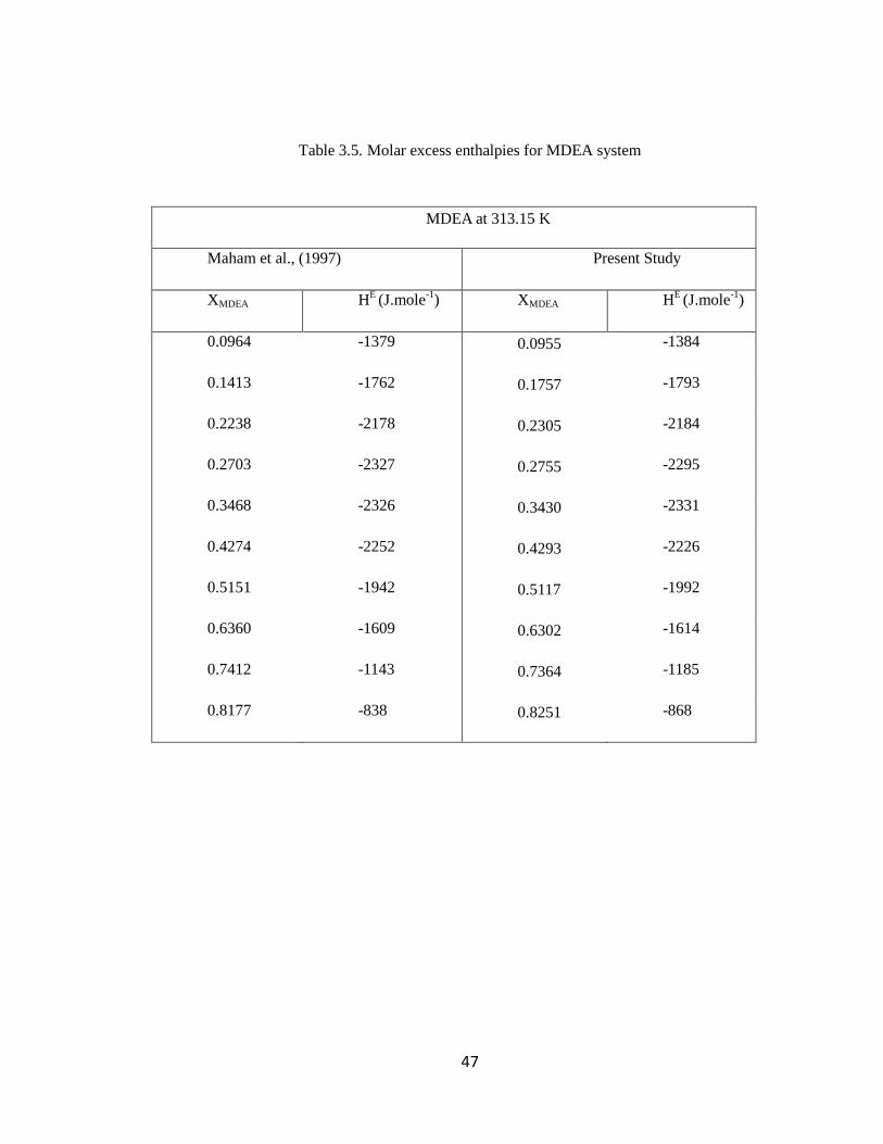
47

Table 3.5. Molar excess enthalpies for MDEA system

MDEA at 313.15 K

Maham et al., (1997) Present Study

XMDEA HE

(J.mole-1

) XMDEA HE

(J.mole-1

)

0.0964 -1379 0.0955 -1384

0.1413 -1762 0.1757 -1793

0.2238 -2178 0.2305 -2184

0.2703 -2327 0.2755 -2295

0.3468 -2326 0.3430 -2331

0.4274 -2252 0.4293 -2226

0.5151 -1942 0.5117 -1992

0.6360 -1609 0.6302 -1614

0.7412 -1143 0.7364 -1185

0.8177 -838 0.8251 -868

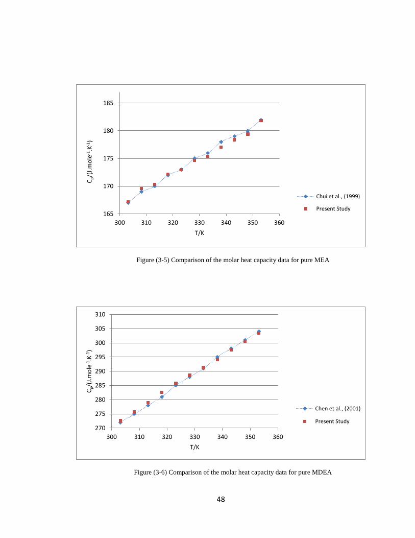
48

Figure (3-5) Comparison of the molar heat capacity data for pure MEA

Figure (3-6) Comparison of the molar heat capacity data for pure MDEA

165

170

175

180

185

300 310 320 330 340 350 360

Cp/(

J.m

ole

-1.K

-1)

T/K

Chui et al., (1999)

Present Study

270

275

280

285

290

295

300

305

310

300 310 320 330 340 350 360

Cp/(

J.m

ole

-1.K

-1)

T/K

Chen et al., (2001)

Present Study

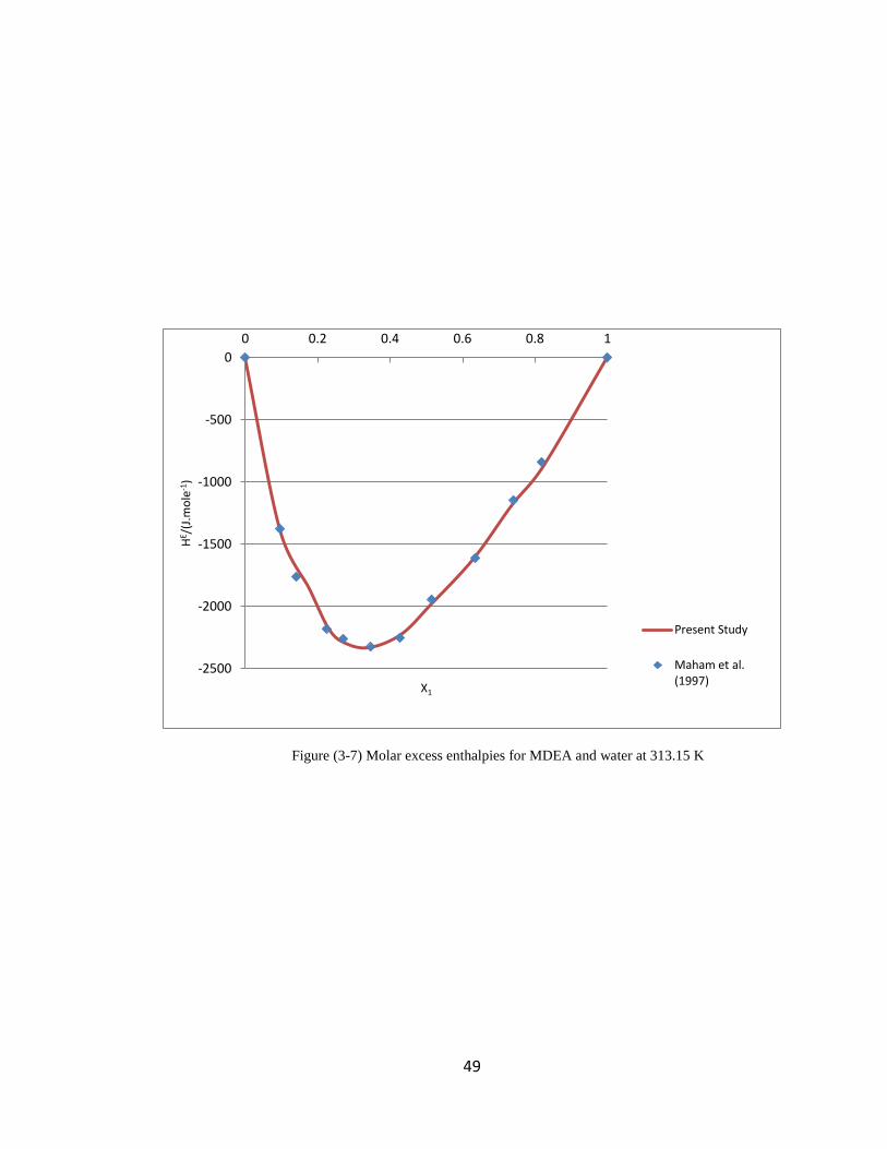
49

Figure (3-7) Molar excess enthalpies for MDEA and water at 313.15 K

-2500

-2000

-1500

-1000

-500

0

0 0.2 0.4 0.6 0.8 1

HE /

(J.m

ole

-1)

X1

Present Study

Maham et al. (1997)

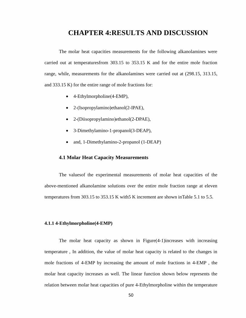
50

CHAPTER 4:RESULTS AND DISCUSSION

The molar heat capacities measurements for the following alkanolamines were

carried out at temperaturesfrom 303.15 to 353.15 K and for the entire mole fraction

range, while, measurements for the alkanolamines were carried out at (298.15, 313.15,

and 333.15 K) for the entire range of mole fractions for:

4-Ethylmorpholine(4-EMP),

2-(Isopropylamino)ethanol(2-IPAE),

2-(Diisopropylamino)ethanol(2-DPAE),

3-Dimethylamino-1-propanol(3-DEAP),

and, 1-Dimethylamino-2-propanol (1-DEAP)

4.1 Molar Heat Capacity Measurements

The valuesof the experimental measurements of molar heat capacities of the

above-mentioned alkanolamine solutions over the entire mole fraction range at eleven

temperatures from 303.15 to 353.15 K with5 K increment are shown in Table 5.1 to 5.5.

4.1.1 4-Ethylmorpholine(4-EMP)

The molar heat capacity as shown in Figure(4-1)increases with increasing

temperature , In addition, the value of molar heat capacity is related to the changes in

mole fractions of 4-EMP by increasing the amount of mole fractions in 4-EMP , the

molar heat capacity increases as well. The linear function shown below represents the

relation between molar heat capacities of pure 4-Ethylmorpholine within the temperature

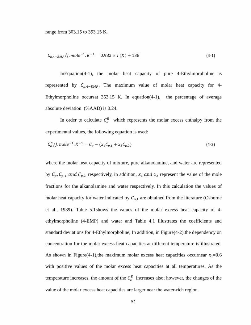
51

range from 303.15 to 353.15 K.

(4-1)

InEquation (4-1), the molar heat capacity of pure 4-Ethylmorpholine is

represented by . The maximum value of molar heat capacity for 4-

Ethylmorpholine occursat 353.15 K. In equation (4-1), the percentage of average

absolute deviation (%AAD) is 0.24.

In order to calculate which represents the molar excess enthalpy from the

experimental values, the following equation is used:

(4-2)

where the molar heat capacity of mixture, pure alkanolamine, and water are represented

by respectively, in addition, represent the value of the mole

fractions for the alkanolamine and water respectively. In this calculation the values of

molar heat capacity for water indicated by are obtained from the literature (Osborne

et al., 1939). Table 5.1shows the values of the molar excess heat capacity of 4-

ethylmorpholine (4-EMP) and water and Table 4.1 illustrates the coefficients and

standard deviations for 4-Ethylmorpholine, In addition, in Figure(4-2),the dependency on

concentration for the molar excess heat capacities at different temperature is illustrated.

As shown in Figure(4-1),the maximum molar excess heat capacities occurnear x1=0.6

with positive values of the molar excess heat capacities at all temperatures. As the

temperature increases, the amount of the increases also; however, the changes of the

value of the molar excess heat capacities are larger near the water-rich region.

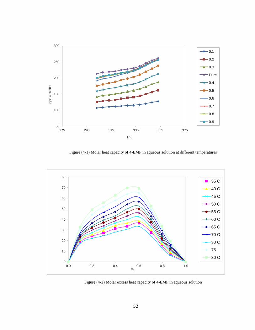
52

Figure (4-1) Molar heat capacity of 4-EMP in aqueous solution at different temperatures

Figure (4-2) Molar excess heat capacity of 4-EMP in aqueous solution

50

100

150

200

250

300

275 295 315 335 355 375

Cp/J

.mole

-1K

-1

T/K

0.1

0.2

0.3

Pure

0.4

0.5

0.6

0.7

0.8

0.9

0

10

20

30

40

50

60

70

80

0.0 0.2 0.4 0.6 0.8 1.0

35 C

40 C

45 C

50 C

55 C

60 C

65 C

70 C

30 C

75

80 C

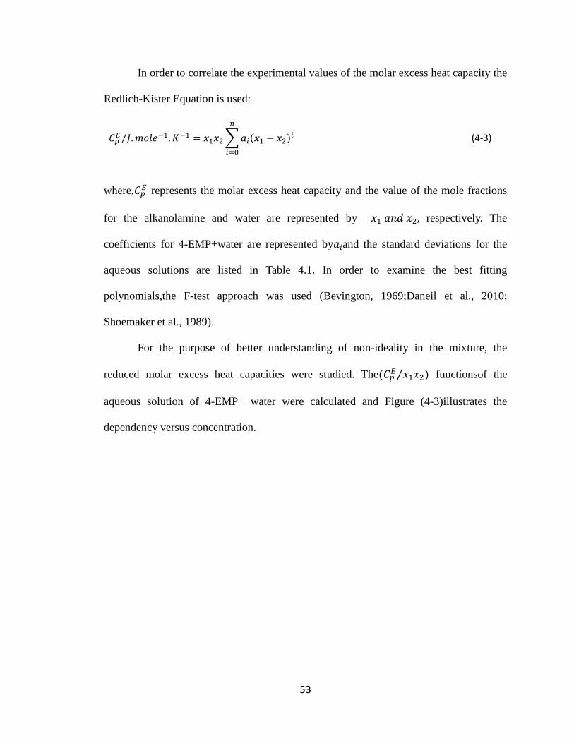
53

In order to correlate the experimental values of the molar excess heat capacity the

Redlich-Kister Equation is used:

(4-3)

where, represents the molar excess heat capacity and the value of the mole fractions

for the alkanolamine and water are represented by respectively. The

coefficients for 4-EMP+water are represented by and the standard deviations for the

aqueous solutions are listed in Table 4.1. In order to examine the best fitting

polynomials,the F-test approach was used (Bevington, 1969;Daneil et al., 2010;

Shoemaker et al., 1989).

For the purpose of better understanding of non-ideality in the mixture, the

reduced molar excess heat capacities were studied. The functionsof the

aqueous solution of 4-EMP+ water were calculated and Figure (4-3)illustrates the

dependency versus concentration.

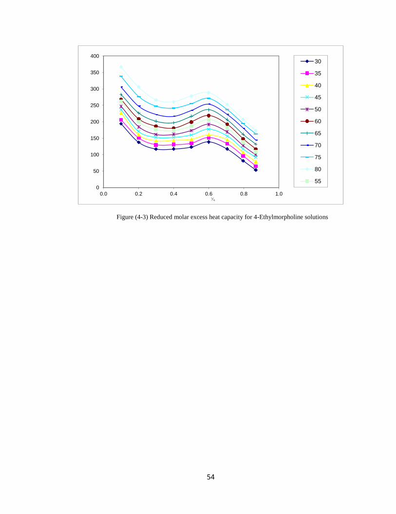
54

Figure (4-3) Reduced molar excess heat capacity for 4-Ethylmorpholine solutions

0

50

100

150

200

250

300

350

400

0.0 0.2 0.4 0.6 0.8 1.0

30

35

40

45

50

60

65

70

75

80

55

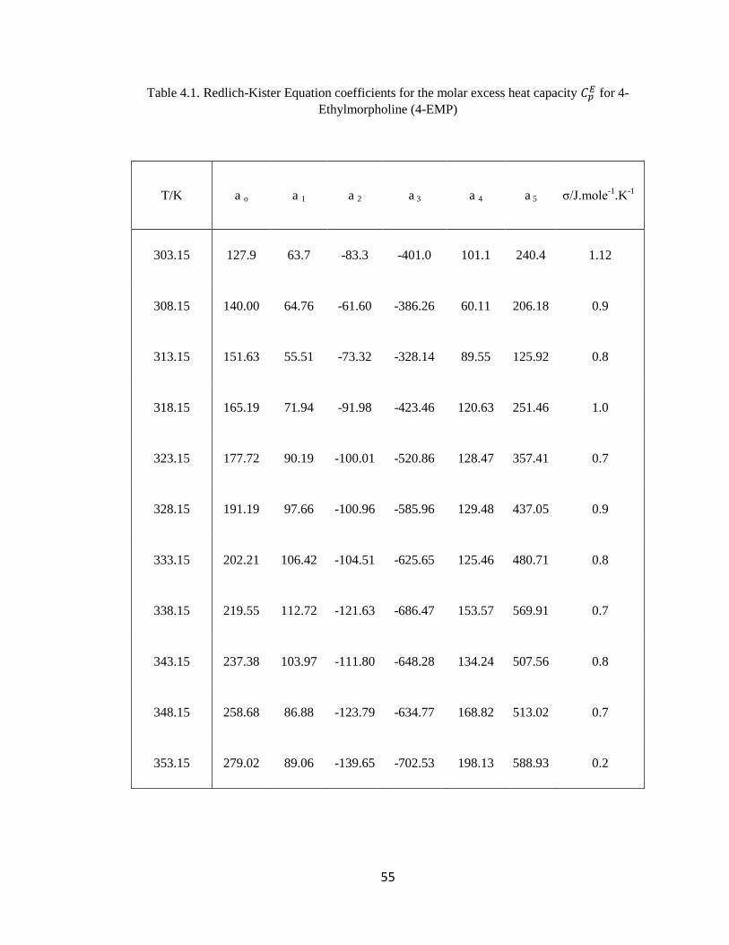
55

Table 4.1. Redlich-Kister Equation coefficients for the molar excess heat capacity for 4-

Ethylmorpholine (4-EMP)

T/K a o a 1 a 2 a 3 a 4 a 5 σ/J.mole-1

.K-1

303.15 127.9 63.7 -83.3 -401.0 101.1 240.4 1.12

308.15 140.00 64.76 -61.60 -386.26 60.11 206.18 0.9

313.15 151.63 55.51 -73.32 -328.14 89.55 125.92 0.8

318.15 165.19 71.94 -91.98 -423.46 120.63 251.46 1.0

323.15 177.72 90.19 -100.01 -520.86 128.47 357.41 0.7

328.15 191.19 97.66 -100.96 -585.96 129.48 437.05 0.9

333.15 202.21 106.42 -104.51 -625.65 125.46 480.71 0.8

338.15 219.55 112.72 -121.63 -686.47 153.57 569.91 0.7

343.15 237.38 103.97 -111.80 -648.28 134.24 507.56 0.8

348.15 258.68 86.88 -123.79 -634.77 168.82 513.02 0.7

353.15 279.02 89.06 -139.65 -702.53 198.13 588.93 0.2

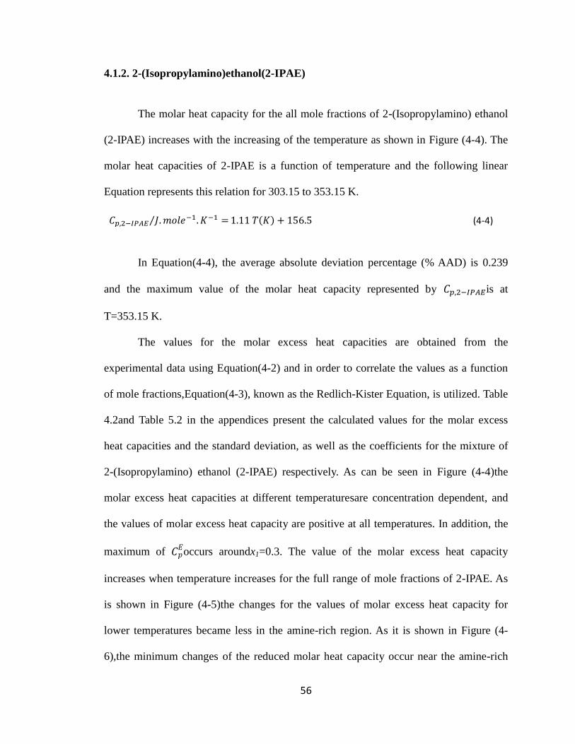
56

4.1.2. 2-(Isopropylamino)ethanol(2-IPAE)

The molar heat capacity for the all mole fractions of 2-(Isopropylamino) ethanol

(2-IPAE) increases with the increasing of the temperature as shown in Figure (4-4). The

molar heat capacities of 2-IPAE is a function of temperature and the following linear

Equation represents this relation for 303.15 to 353.15 K.

(4-4)

In Equation (4-4), the average absolute deviation percentage (% AAD) is 0.239

and the maximum value of the molar heat capacity represented by is at

T=353.15 K.

The values for the molar excess heat capacities are obtained from the

experimental data using Equation (4-2) and in order to correlate the values as a function

of mole fractions,Equation (4-3), known as the Redlich-Kister Equation, is utilized. Table

4.2and Table 5.2 in the appendices present the calculated values for the molar excess

heat capacities and the standard deviation, as well as the coefficients for the mixture of

2-(Isopropylamino) ethanol (2-IPAE) respectively. As can be seen in Figure (4-4)the

molar excess heat capacities at different temperaturesare concentration dependent, and

the values of molar excess heat capacity are positive at all temperatures. In addition, the

maximum of occurs aroundx1=0.3. The value of the molar excess heat capacity

increases when temperature increases for the full range of mole fractions of 2-IPAE. As

is shown in Figure (4-5)the changes for the values of molar excess heat capacity for

lower temperatures became less in the amine-rich region. As it is shown in Figure (4-

6),the minimum changes of the reduced molar heat capacity occur near the amine-rich

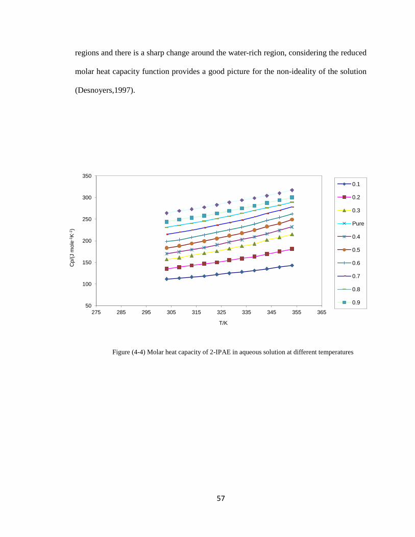
57

regions and there is a sharp change around the water-rich region, considering the reduced

molar heat capacity function provides a good picture for the non-ideality of the solution

(Desnoyers,1997).

Figure (4-4) Molar heat capacity of 2-IPAE in aqueous solution at different temperatures

50

100

150

200

250

300

350

275 285 295 305 315 325 335 345 355 365

Cp/(

J m

ole

-1K

-1)

T/K

0.1

0.2

0.3

Pure

0.4

0.5

0.6

0.7

0.8

0.9

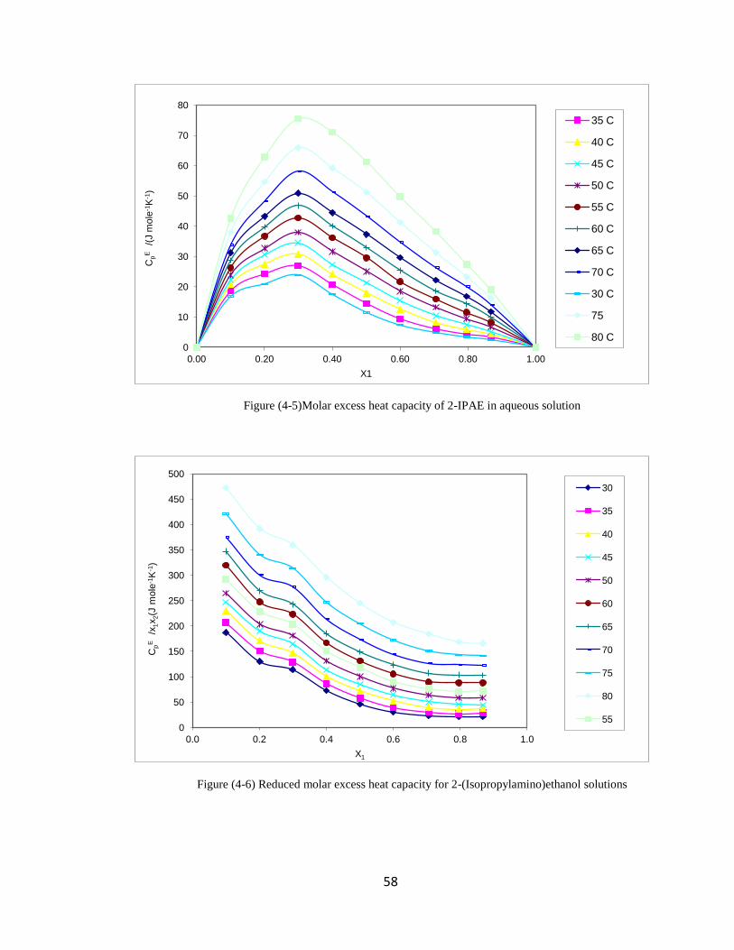
58

Figure (4-5)Molar excess heat capacity of 2-IPAE in aqueous solution

Figure (4-6) Reduced molar excess heat capacity for 2-(Isopropylamino)ethanol solutions

0

10

20

30

40

50

60

70

80

0.00 0.20 0.40 0.60 0.80 1.00

Cp

E /

(J m

ole

-1K

-1)

X1

35 C

40 C

45 C

50 C

55 C

60 C

65 C

70 C

30 C

75

80 C

0

50

100

150

200

250

300

350

400

450

500

0.0 0.2 0.4 0.6 0.8 1.0

Cp

E /

x1x

2(J

mole

-1K

-1)

X1

30

35

40

45

50

60

65

70

75

80

55

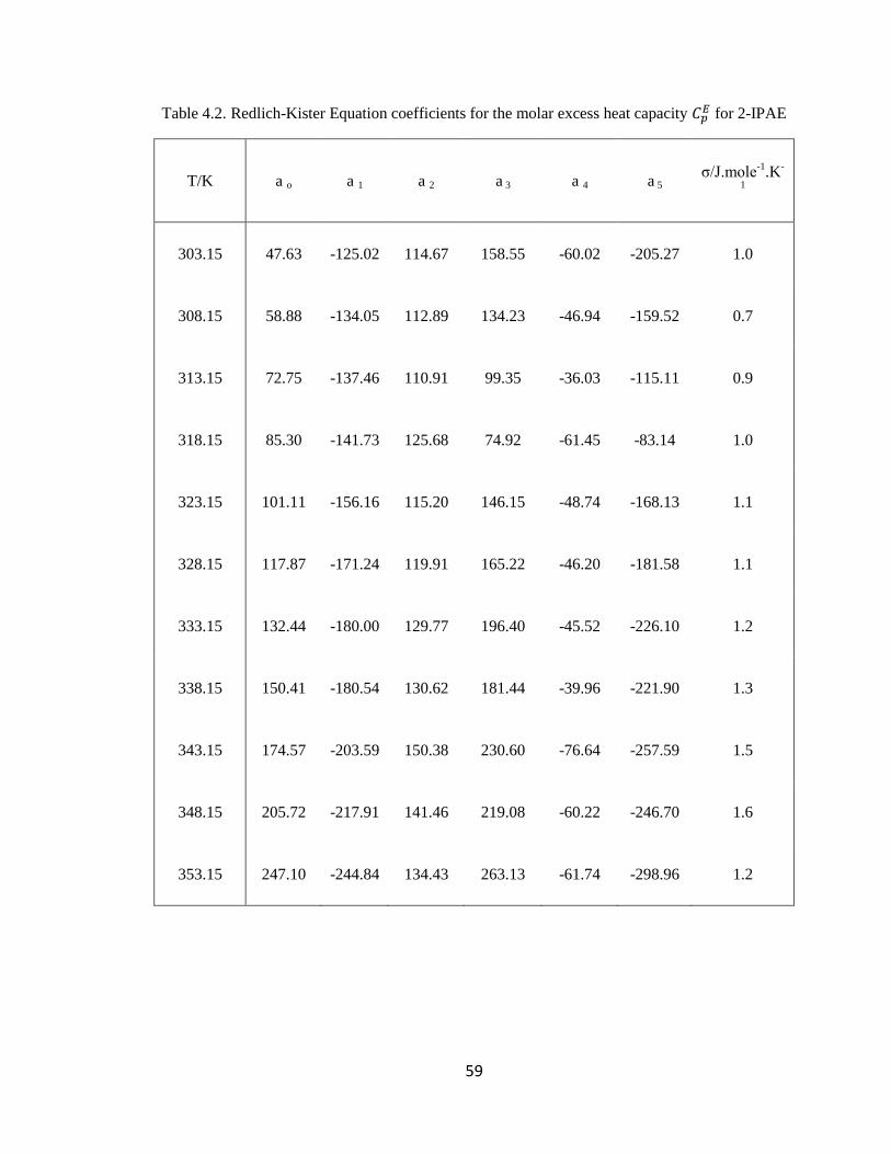
59

Table 4.2. Redlich-Kister Equation coefficients for the molar excess heat capacity for 2-IPAE

T/K a o a 1 a 2 a 3 a 4 a 5 σ/J.mole

-1.K

-

1

303.15 47.63 -125.02 114.67 158.55 -60.02 -205.27 1.0

308.15 58.88 -134.05 112.89 134.23 -46.94 -159.52 0.7

313.15 72.75 -137.46 110.91 99.35 -36.03 -115.11 0.9

318.15 85.30 -141.73 125.68 74.92 -61.45 -83.14 1.0

323.15 101.11 -156.16 115.20 146.15 -48.74 -168.13 1.1

328.15 117.87 -171.24 119.91 165.22 -46.20 -181.58 1.1

333.15 132.44 -180.00 129.77 196.40 -45.52 -226.10 1.2

338.15 150.41 -180.54 130.62 181.44 -39.96 -221.90 1.3

343.15 174.57 -203.59 150.38 230.60 -76.64 -257.59 1.5

348.15 205.72 -217.91 141.46 219.08 -60.22 -246.70 1.6

353.15 247.10 -244.84 134.43 263.13 -61.74 -298.96 1.2

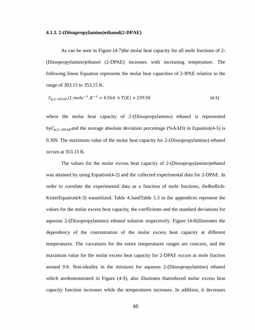
60

4.1.3. 2-(Diisopropylamino)ethanol(2-DPAE)

As can be seen in Figure (4-7)the molar heat capacity for all mole fractions of 2-

(Diisopropylamino)ethanol (2-DPAE) increases with increasing temperature. The

following linear Equation represents the molar heat capacities of 2-IPAE relation in the

range of 303.15 to 353.15 K.

(4-5)

where the molar heat capacity of 2-(Diisopropylamino) ethanol is represented

by and the average absolute deviation percentage (%AAD) in Equation‎(4-5) is

0.309. The maximum value of the molar heat capacity for 2-(Dissopropylamino) ethanol

occurs at 353.15 K.

The values for the molar excess heat capacity of 2-(Dissopropylamino)ethanol

was attained by using Equation‎(4-2) and the collected experimental data for 2-DPAE. In

order to correlate the experimental data as a function of mole fractions, theRedlich-

KisterEquation‎(4-3) wasutilized. ‎Table 4.3and‎Table 5.3 in the appendices represent the

values for the molar excess heat capacity, the coefficients and the standard deviations for

aqueous 2-(Diisopropylamino) ethanol solution respectively. Figure (4-8)illustrates the

dependency of the concentration of the molar excess heat capacity at different

temperatures. The curvatures for the entire temperatures ranges are concave, and the

maximum value for the molar excess heat capacity for 2-DPAE occurs at mole fraction

around 0.6. Non-ideality in the mixtures for aqueous 2-(Dissopropylamino) ethanol

which aredemonstrated in Figure (4-9), also illustrates thatreduced molar excess heat

capacity function increases while the temperatures increases. In addition, it decreases

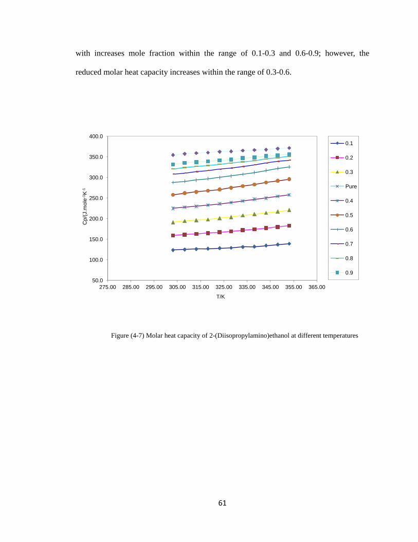
61

with increases mole fraction within the range of 0.1-0.3 and 0.6-0.9; however, the

reduced molar heat capacity increases within the range of 0.3-0.6.

Figure (4-7) Molar heat capacity of 2-(Diisopropylamino)ethanol at different temperatures

50.0

100.0

150.0

200.0

250.0

300.0

350.0

400.0

275.00 285.00 295.00 305.00 315.00 325.00 335.00 345.00 355.00 365.00

Cp/(

J.m

ole

-1K

-1

T/K

0.1

0.2

0.3

Pure

0.4

0.5

0.6

0.7

0.8

0.9

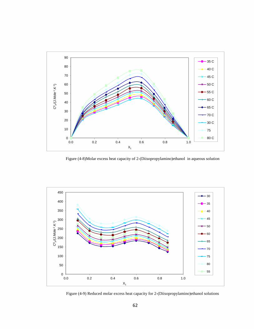
62

Figure (4-8)Molar excess heat capacity of 2-(Diisopropylamino)ethanol in aqueous solution

Figure (4-9) Reduced molar excess heat capacity for 2-(Diisopropylamino)ethanol solutions

0

10

20

30

40

50

60

70

80

90

0.0 0.2 0.4 0.6 0.8 1.0

CE

P/(

J.M

ole

-1.K

-1)

X1

35 C

40 C

45 C

50 C

55 C

60 C

65 C

70 C

30 C

75

80 C

0

50

100

150

200

250

300

350

400

450

0.0 0.2 0.4 0.6 0.8 1.0

CE

P/(

J.M

ole

-1.K

-1)

X1

30

35

40

45

50

60

65

70

75

80

55

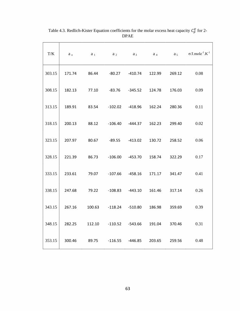
63

Table 4.3. Redlich-Kister Equation coefficients for the molar excess heat capacity for 2-

DPAE

T/K a o a 1 a 2 a 3 a 4 a 5 σ/J.mole-1

.K-1

303.15 171.74 86.44 -80.27 -410.74 122.99 269.12 0.08

308.15 182.13 77.10 -83.76 -345.52 124.78 176.03 0.09

313.15 189.91 83.54 -102.02 -418.96 162.24 280.36 0.11

318.15 200.13 88.12 -106.40 -444.37 162.23 299.40 0.02

323.15 207.97 80.67 -89.55 -413.02 130.72 258.52 0.06

328.15 221.39 86.73 -106.00 -453.70 158.74 322.29 0.17

333.15 233.61 79.07 -107.66 -458.16 171.17 341.47 0.41

338.15 247.68 79.22 -108.83 -443.10 161.46 317.14 0.26

343.15 267.16 100.63 -118.24 -510.80 186.98 359.69 0.39

348.15 282.25 112.10 -110.52 -543.66 191.04 370.46 0.31

353.15 300.46 89.75 -116.55 -446.85 203.65 259.56 0.48

64

4.1.4. 3-Dimethylamino-1-propanol(3-DEAP)

Figure (4-9a) shows that the molar heat capacity for all mole fractions of 3-

Dimethylamino-1-propanol (3-DEAP) increases with increasing temperature. The

following linear Equation represents the molar heat capacities of 3-DEAP in relation to

temperature changes for the range of 303.15 to 353.15 K.

(4-6)

where, presents the molar heat capacity of 3-Dimethylamino-1-propanol (3-

DEAP). Moreover, the percentage of AAD which stands for average absolute deviation

in Equation (4-6) is around 0.259, whereas at a temperature of 353.15 K, the maximum

value of the molar heat capacity for 3-Dimethylamino-1-propanol (3-DEAP) occurs.

For the purpose of obtaining the value of the molar excess heat capacity of 3-

Dimethylamino-1-propanol (3-DEAP) Equation (4-2) was used along with the obtained

data from the experiments. In order to correlate the experimental data as a function of

mole fraction the Redlich-KisterEquation (4-3) was employed, and the obtained value for

the molar excess heat capacity for aqueous solution of 3-Dimethylamino-1-propanol (3-

DEAP) along with the coefficients and the standard deviations are shown in Table 5.4and

Table 4.4, respectively.

Figure (4-10) shows the dependency of the concentration for the molar excess

heat capacity at different temperatures.Furthermore, it is noticeable that the values at all

temperatures are positive and at a mole fraction of 0.4, the maximum value of the mole

excess heat capacity for 3-DEAP occurs. It is apparentfrom Figure (4-11)that the amount

of reduced molar excess heat capacity becomes greater with increasing temperature.

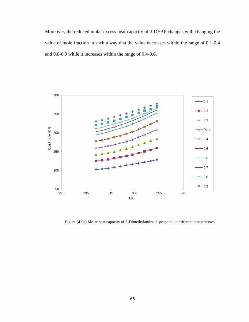
65

Moreover, the reduced molar excess heat capacity of 3-DEAP changes with changing the

value of mole fraction in such a way that the value decreases within the range of 0.1-0.4

and 0.6-0.9 while it increases within the range of 0.4-0.6.

Figure (4-9a) Molar heat capacity of 3-Dimethylamino-1-propanol at different temperatures

50

100

150

200

250

300

275 295 315 335 355 375

Cp/(

J.m

ole

-1K

-1)

T/K

0.1

0.2

0.3

Pure

0.4

0.5

0.6

0.7

0.8

0.9

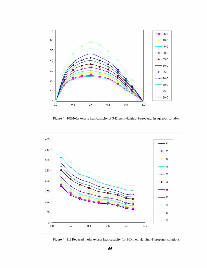
66

Figure (4-10)Molar excess heat capacity of 3-Dimethylamino-1-propanol in aqueous solution

Figure (4-11) Reduced molar excess heat capacity for 3-Dimethylamino-1-propanol solutions

0

10

20

30

40

50

60

70

0.0 0.2 0.4 0.6 0.8 1.0

35 C

40 C

45 C

50 C

55 C

60 C

65 C

70 C

30 C

75

80 C

0

50

100

150

200

250

300

350

400

0.0 0.2 0.4 0.6 0.8 1.0

30

35

40

45

50

60

65

70

75

80

55

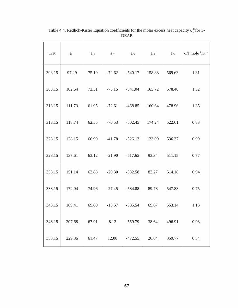
67

Table 4.4. Redlich-Kister Equation coefficients for the molar excess heat capacity for 3-

DEAP

T/K a o a 1 a 2 a 3 a 4 a 5 σ/J.mole-1

.K-1

303.15 97.29 75.19 -72.62 -540.17 158.88 569.63 1.31

308.15 102.64 73.51 -75.15 -541.04 165.72 578.40 1.32

313.15 111.73 61.95 -72.61 -468.85 160.64 478.96 1.35

318.15 118.74 62.55 -70.53 -502.45 174.24 522.61 0.83

323.15 128.15 66.90 -41.78 -526.12 123.00 536.37 0.99

328.15 137.61 63.12 -21.90 -517.65 93.34 511.15 0.77

333.15 151.14 62.88 -20.30 -532.58 82.27 514.18 0.94

338.15 172.04 74.96 -27.45 -584.88 89.78 547.88 0.75

343.15 189.41 69.60 -13.57 -585.54 69.67 553.14 1.13

348.15 207.68 67.91 8.12 -559.79 38.64 496.91 0.93

353.15 229.36 61.47 12.08 -472.55 26.84 359.77 0.34

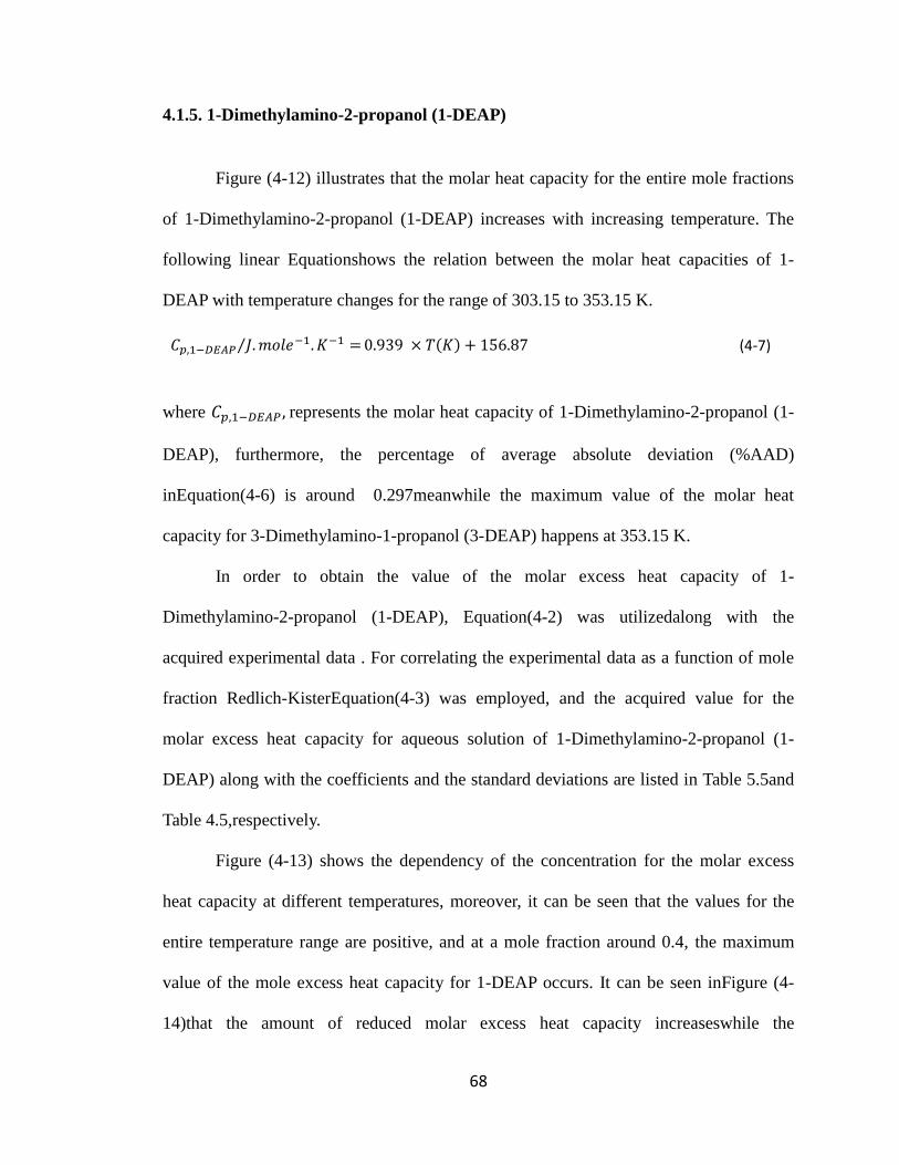
68

4.1.5. 1-Dimethylamino-2-propanol (1-DEAP)

Figure (4-12) illustrates that the molar heat capacity for the entire mole fractions

of 1-Dimethylamino-2-propanol (1-DEAP) increases with increasing temperature. The

following linear Equationshows the relation between the molar heat capacities of 1-

DEAP with temperature changes for the range of 303.15 to 353.15 K.

(4-7)

where represents the molar heat capacity of 1-Dimethylamino-2-propanol (1-

DEAP), furthermore, the percentage of average absolute deviation (%AAD)

inEquation (4-6) is around 0.297meanwhile the maximum value of the molar heat

capacity for 3-Dimethylamino-1-propanol (3-DEAP) happens at 353.15 K.

In order to obtain the value of the molar excess heat capacity of 1-

Dimethylamino-2-propanol (1-DEAP), Equation (4-2) was utilizedalong with the

acquired experimental data . For correlating the experimental data as a function of mole

fraction Redlich-KisterEquation (4-3) was employed, and the acquired value for the

molar excess heat capacity for aqueous solution of 1-Dimethylamino-2-propanol (1-

DEAP) along with the coefficients and the standard deviations are listed in Table 5.5and

Table 4.5,respectively.

Figure (4-13) shows the dependency of the concentration for the molar excess

heat capacity at different temperatures, moreover, it can be seen that the values for the

entire temperature range are positive, and at a mole fraction around 0.4, the maximum

value of the mole excess heat capacity for 1-DEAP occurs. It can be seen inFigure (4-

14)that the amount of reduced molar excess heat capacity increaseswhile the

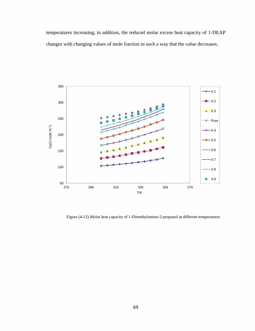
69

temperatures increasing, in addition, the reduced molar excess heat capacity of 1-DEAP

changes with changing values of mole fraction in such a way that the value decreases.

Figure (4-12) Molar heat capacity of 1-Dimethylamino-2-propanol at different temperatures

50

100

150

200

250

300

350

275 295 315 335 355 375

Cp/(

J m

ole

-1K

-1)

T/K

0.1

0.2

0.3

Pure

0.4

0.5

0.6

0.7

0.8

0.9

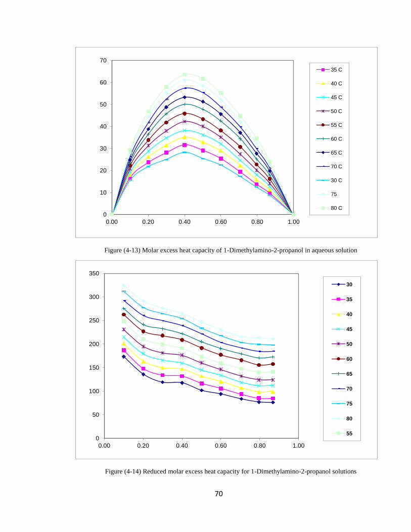
70

Figure (4-13) Molar excess heat capacity of 1-Dimethylamino-2-propanol in aqueous solution

Figure (4-14) Reduced molar excess heat capacity for 1-Dimethylamino-2-propanol solutions

0

10

20

30

40

50

60

70

0.00 0.20 0.40 0.60 0.80 1.00

35 C

40 C

45 C

50 C

55 C

60 C

65 C

70 C

30 C

75

80 C

0

50

100

150

200

250

300

350

0.00 0.20 0.40 0.60 0.80 1.00

30

35

40

45

50

60

65

70

75

80

55

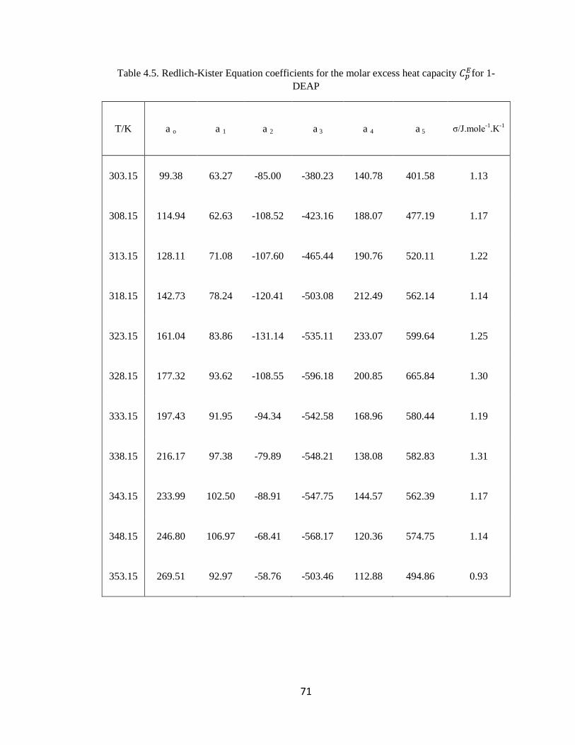
71

Table 4.5. Redlich-Kister Equation coefficients for the molar excess heat capacity for 1-

DEAP

T/K a o a 1 a 2 a 3 a 4 a 5 σ/J.mole-1

.K-1

303.15 99.38 63.27 -85.00 -380.23 140.78 401.58 1.13

308.15 114.94 62.63 -108.52 -423.16 188.07 477.19 1.17

313.15 128.11 71.08 -107.60 -465.44 190.76 520.11 1.22

318.15 142.73 78.24 -120.41 -503.08 212.49 562.14 1.14

323.15 161.04 83.86 -131.14 -535.11 233.07 599.64 1.25

328.15 177.32 93.62 -108.55 -596.18 200.85 665.84 1.30

333.15 197.43 91.95 -94.34 -542.58 168.96 580.44 1.19

338.15 216.17 97.38 -79.89 -548.21 138.08 582.83 1.31

343.15 233.99 102.50 -88.91 -547.75 144.57 562.39 1.17

348.15 246.80 106.97 -68.41 -568.17 120.36 574.75 1.14

353.15 269.51 92.97 -58.76 -503.46 112.88 494.86 0.93

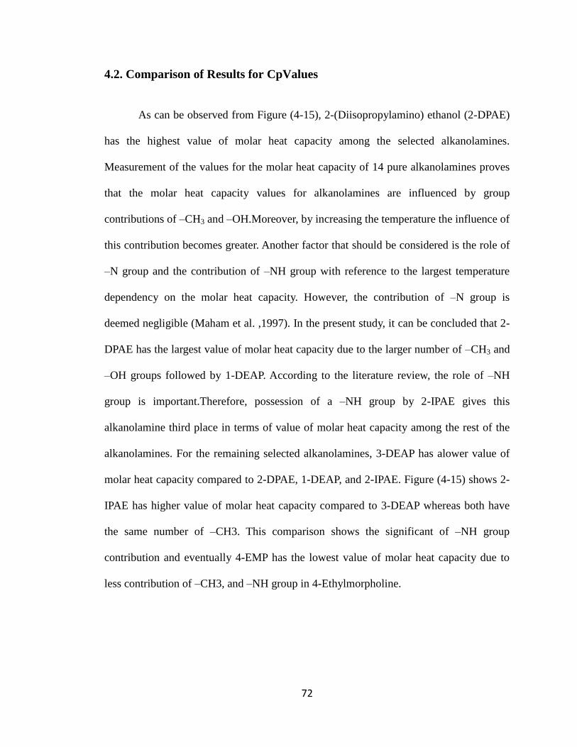
72

4.2. Comparison of Results for CpValues

As can be observed from Figure (4-15), 2-(Diisopropylamino) ethanol (2-DPAE)

has the highest value of molar heat capacity among the selected alkanolamines.

Measurement of the values for the molar heat capacity of 14 pure alkanolamines proves

that the molar heat capacity values for alkanolamines are influenced by group

contributions of –CH3 and –OH.Moreover, by increasing the temperature the influence of

this contribution becomes greater. Another factor that should be considered is the role of

–N group and the contribution of –NH group with reference to the largest temperature

dependency on the molar heat capacity. However, the contribution of –N group is

deemed negligible (Maham et al. ,1997). In the present study, it can be concluded that 2-

DPAE has the largest value of molar heat capacity due to the larger number of –CH3 and

–OH groups followed by 1-DEAP. According to the literature review, the role of –NH

group is important.Therefore, possession of a –NH group by 2-IPAE gives this

alkanolamine third place in terms of value of molar heat capacity among the rest of the

alkanolamines. For the remaining selected alkanolamines, 3-DEAP has alower value of

molar heat capacity compared to 2-DPAE, 1-DEAP, and 2-IPAE. Figure (4-15) shows 2-

IPAE has higher value of molar heat capacity compared to 3-DEAP whereas both have

the same number of –CH3. This comparison shows the significant of –NH group

contribution and eventually 4-EMP has the lowest value of molar heat capacity due to

less contribution of –CH3, and –NH group in 4-Ethylmorpholine.

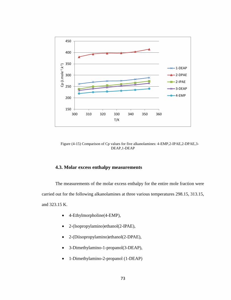
73

Figure (4-15) Comparison of Cp values for five alkanolamines: 4-EMP,2-IPAE,2-DPAE,3-

DEAP,1-DEAP

4.3. Molar excess enthalpy measurements

The measurements of the molar excess enthalpy for the entire mole fraction were

carried out for the following alkanolamines at three various temperatures 298.15, 313.15,

and 323.15 K.

4-Ethylmorpholine(4-EMP),

2-(Isopropylamino)ethanol(2-IPAE),

2-(Diisopropylamino)ethanol(2-DPAE),

3-Dimethylamino-1-propanol(3-DEAP),

1-Dimethylamino-2-propanol (1-DEAP)

150

200

250

300

350

400

450

300 310 320 330 340 350 360

Cp

(J.

mo

le-1

.k-1

)

T/K

1-DEAP

2-DPAE

2-IPAE

3-DEAP

4-EMP

74

The correlation of the empirical data was done as a function of the mole fractions

by means of the Redlich-KisterEquation (4-3). Maham’s method was used in order to

determine the values of the enthalpy for the solution of alkanolamines and water

(Maham et al,.1997). Finally, the NRTL (Non-Random Two Liquid), UNIQUAC

(Universal Quasi-Chemical) and UNIFAC (Universal Functional Activity Coefficient)

models were used to model the acquired data for the molar excess enthalpies.

4.3.1. 4-Ethylmorpholine(4-EMP)

The measurements of molar excess enthalpies for 4-Ethylmorpholine (4-EMP)

were carried out at three temperatures: 298.15, 313.15, and 323.15 K. Table 5.6and

Figure (4-16)illustrates the dependency of the mole fractions at different temperatures of

the calculated molar excess enthalpy values. As can be seen fromFigure (4-16), the

minimum molar enthalpy excess value occurs at x=0.3 and the curve is shown in Figure

(4-16) is negative which proves that an exothermic mixing process happened between 4-

Ethylmorpholine (4-EMP) and water. The interaction of the amine group in 4-

Ethylmorpholine and –OH group in water is probablythe main cause of the exothermic

mixing process.

The comparison between aqueous ethanol and diethylamine in terms of the molar

excess enthalpies value shows that the interaction between –OH group of water with the

amine group of diethylamine is more effective compared to the –OH group of

water.Therefore, the reverse effect on the molar excess enthalpies for the binary aqueous

solution with respect to the amine groups and ethanol should be considered (Maham et

al., 1997). Another comparison was made between diethanolamineand

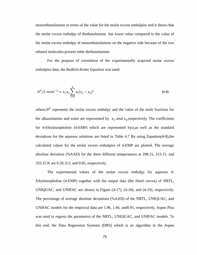
75

monoethanolamine in terms of the value for the molar excess enthalpies and it shows that

the molar excess enthalpy of diethanolamine has lower value compared to the value of

the molar excess enthalpy of monoethanolamine on the negative side because of the two

ethanol molecules present inthe diethanolamine.

For the purpose of correlation of the experimentally acquired molar excess

enthalpies data, the Redlich-Kister Equation was used:

(4-8)

where, represents the molar excess enthalpy and the value of the mole fractions for

the alkanolamine and water are represented by respectively. The coefficients

for 4-Ethylmorpholine (4-EMP) which are represented by as well as the standard

deviations for the aqueous solutions are listed in Table 4.7 By using Equation (4-8),the

calculated values for the molar excess enthalpies of 4-EMP are plotted. The average

absolute deviation (%AAD) for the three different temperatures at 298.15, 313.15, and

333.15 K are 0.28, 0.5, and 0.85, respectively.

The experimental values of the molar excess enthalpy for aqueous 4-

Ethylmorpholine (4-EMP) together with the output data (the fitted curves) of NRTL,

UNIQUAC, and UNIFAC are shown in Figure (4-17), (4-18), and (4-19), respectively.

The percentage of average absolute deviations (%AAD) of the NRTL, UNIQUAC, and

UNIFAC models for the empirical data are 1.96, 1.66, and0.91, respectively. Aspen Plus

was used to regress the parameters of the NRTL, UNIQUAC, and UNIFAC models. To

this end, the Data Regression Systems (DRS) which is an algorithm in the Aspen

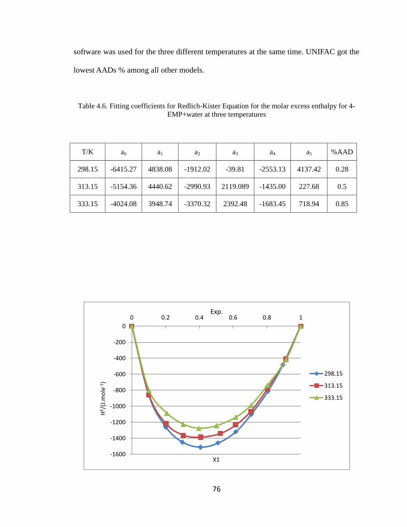
76

software was used for the three different temperatures at the same time. UNIFAC got the

lowest AADs % among all other models.

Table 4.6. Fitting coefficients for Redlich-Kister Equation for the molar excess enthalpy for 4-

EMP+water at three temperatures

T/K a0 a1 a2 a3 a4 a5 %AAD

298.15 -6415.27 4838.08 -1912.02 -39.81 -2553.13 4137.42 0.28

313.15 -5154.36 4440.62 -2990.93 2119.089 -1435.00 227.68 0.5

333.15 -4024.08 3948.74 -3370.32 2392.48 -1683.45 718.94 0.85

-1600

-1400

-1200

-1000

-800

-600

-400

-200

0

0 0.2 0.4 0.6 0.8 1

HE /

(J.m

ole

-1)

X1

Exp.

298.15

313.15

333.15

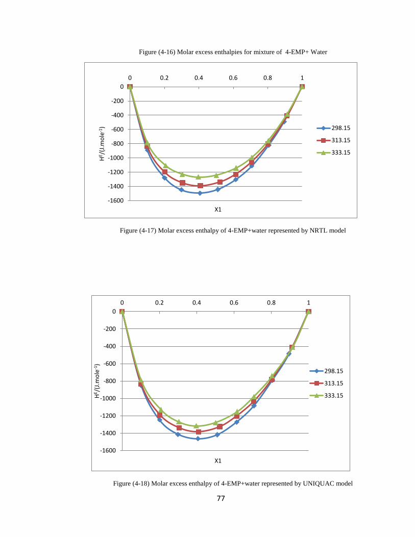
77

Figure (4-16) Molar excess enthalpies for mixture of 4-EMP+ Water

Figure (4-17) Molar excess enthalpy of 4-EMP+water represented by NRTL model

Figure (4-18) Molar excess enthalpy of 4-EMP+water represented by UNIQUAC model

-1600

-1400

-1200

-1000

-800

-600

-400

-200

0

0 0.2 0.4 0.6 0.8 1

HE /

(J.m

ole

-1)

X1

298.15

313.15

333.15

-1600

-1400

-1200

-1000

-800

-600

-400

-200

0

0 0.2 0.4 0.6 0.8 1

HE /

(J.m

ole

-1)

X1

298.15

313.15

333.15

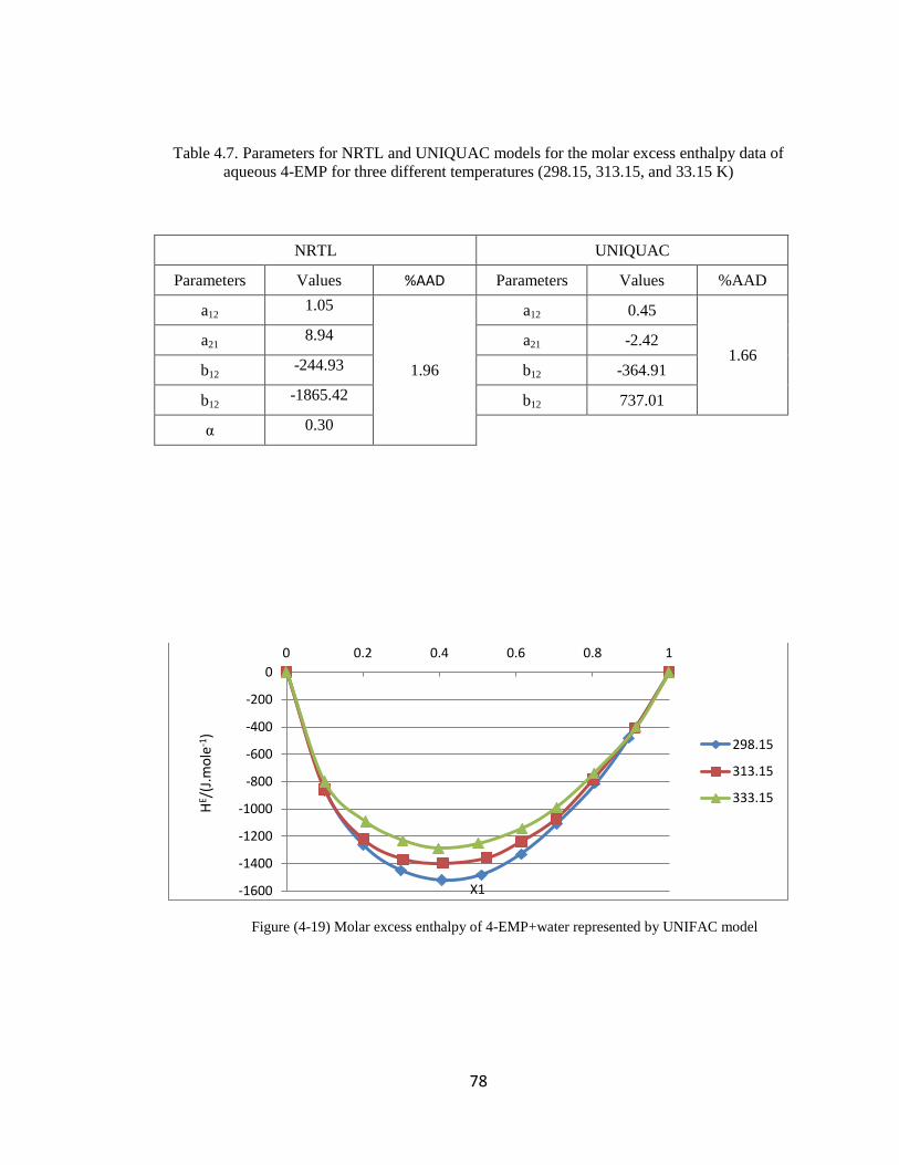
78

Table 4.7. Parameters for NRTL and UNIQUAC models for the molar excess enthalpy data of

aqueous 4-EMP for three different temperatures (298.15, 313.15, and 33.15 K)

NRTL UNIQUAC

Parameters Values %AAD Parameters Values %AAD

a12 1.05

1.96

a12 0.45

1.66 a21

8.94 a21 -2.42

b12 -244.93 b12 -364.91

b12 -1865.42 b12 737.01

α 0.30

Figure (4-19) Molar excess enthalpy of 4-EMP+water represented by UNIFAC model

-1600

-1400

-1200

-1000

-800

-600

-400

-200

0

0 0.2 0.4 0.6 0.8 1

HE /

(J.m

ole

-1)

X1

298.15

313.15

333.15

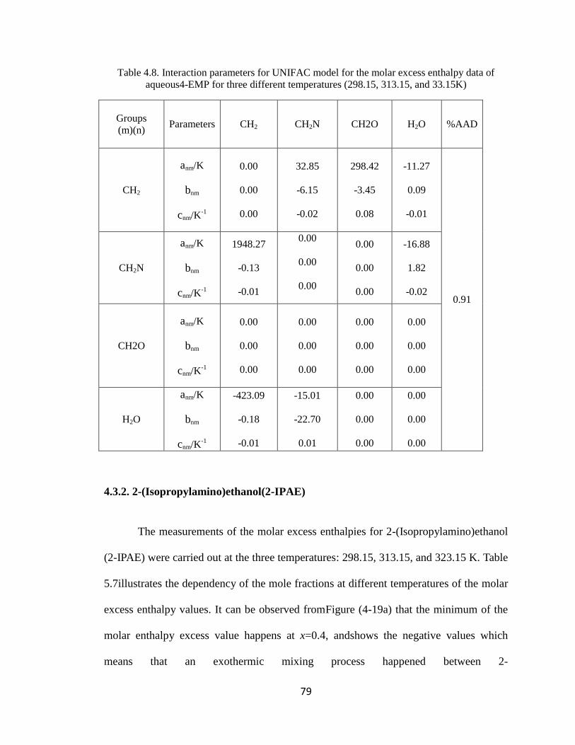
79

Table 4.8. Interaction parameters for UNIFAC model for the molar excess enthalpy data of

aqueous4-EMP for three different temperatures (298.15, 313.15, and 33.15K)

Groups

(m)(n)

Parameters CH2 CH2N CH2O H2O %AAD

CH2

anm/K

bnm

cnm/K-1

0.00

0.00

0.00

32.85

-6.15

-0.02

298.42

-3.45

0.08

-11.27

0.09

-0.01

0.91

CH2N

anm/K

bnm

cnm/K-1

1948.27

-0.13

-0.01

0.00

0.00

0.00

0.00

0.00

0.00

-16.88

1.82

-0.02

CH2O

anm/K

bnm

cnm/K-1

0.00

0.00

0.00

0.00

0.00

0.00

0.00

0.00

0.00

0.00

0.00

0.00

H2O

anm/K

bnm

cnm/K-1

-423.09

-0.18

-0.01

-15.01

-22.70

0.01

0.00

0.00

0.00

0.00

0.00

0.00

4.3.2. 2-(Isopropylamino)ethanol(2-IPAE)

The measurements of the molar excess enthalpies for 2-(Isopropylamino)ethanol

(2-IPAE) were carried out at the three temperatures: 298.15, 313.15, and 323.15 K. Table

5.7illustrates the dependency of the mole fractions at different temperatures of the molar

excess enthalpy values. It can be observed fromFigure (4-19a) that the minimum of the

molar enthalpy excess value happens at x=0.4, andshows the negative values which

means that an exothermic mixing process happened between 2-

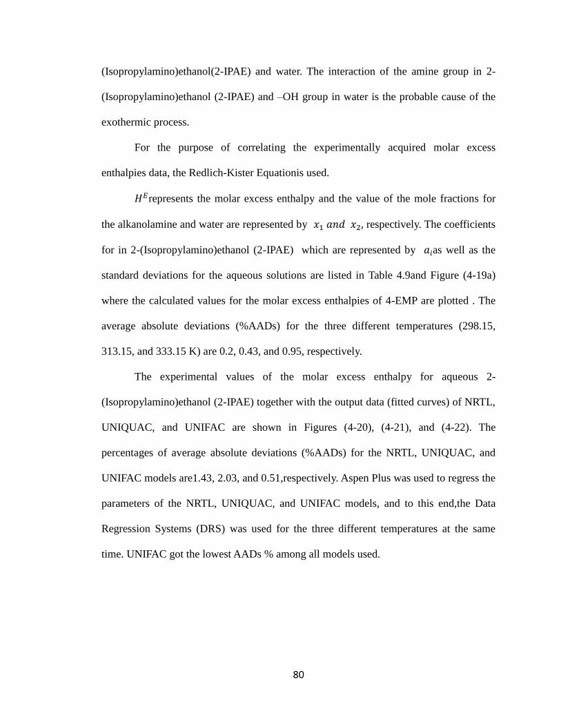
80

(Isopropylamino)ethanol(2-IPAE) and water. The interaction of the amine group in 2-

(Isopropylamino)ethanol (2-IPAE) and –OH group in water is the probable cause of the

exothermic process.

For the purpose of correlating the experimentally acquired molar excess

enthalpies data, the Redlich-Kister Equationis used.

represents the molar excess enthalpy and the value of the mole fractions for

the alkanolamine and water are represented by respectively. The coefficients

for in 2-(Isopropylamino)ethanol (2-IPAE) which are represented by as well as the

standard deviations for the aqueous solutions are listed in Table 4.9and Figure (4-19a)

where the calculated values for the molar excess enthalpies of 4-EMP are plotted . The

average absolute deviations (%AADs) for the three different temperatures (298.15,

313.15, and 333.15 K) are 0.2, 0.43, and 0.95, respectively.

The experimental values of the molar excess enthalpy for aqueous 2-

(Isopropylamino)ethanol (2-IPAE) together with the output data (fitted curves) of NRTL,

UNIQUAC, and UNIFAC are shown in Figures (4-20), (4-21), and (4-22). The

percentages of average absolute deviations (%AADs) for the NRTL, UNIQUAC, and

UNIFAC models are1.43, 2.03, and 0.51,respectively. Aspen Plus was used to regress the

parameters of the NRTL, UNIQUAC, and UNIFAC models, and to this end,the Data

Regression Systems (DRS) was used for the three different temperatures at the same

time. UNIFAC got the lowest AADs % among all models used.

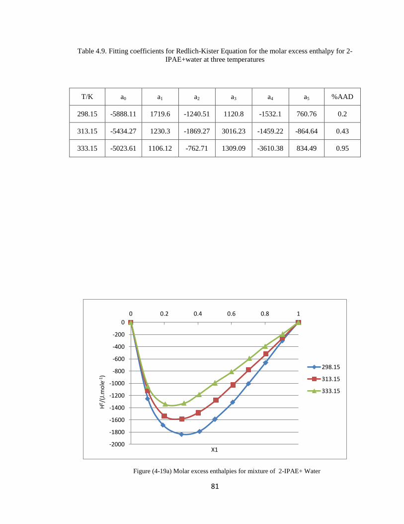
81

Table 4.9. Fitting coefficients for Redlich-Kister Equation for the molar excess enthalpy for 2-

IPAE+water at three temperatures

T/K a0 a1 a2 a3 a4 a5 %AAD

298.15 -5888.11 1719.6 -1240.51 1120.8 -1532.1 760.76 0.2

313.15 -5434.27 1230.3 -1869.27 3016.23 -1459.22 -864.64 0.43

333.15 -5023.61 1106.12 -762.71 1309.09 -3610.38 834.49 0.95

Figure (4-19a) Molar excess enthalpies for mixture of 2-IPAE+ Water

-2000

-1800

-1600

-1400

-1200

-1000

-800

-600

-400

-200

0

0 0.2 0.4 0.6 0.8 1

HE /

(J.m

ole

-1)

X1

298.15

313.15

333.15

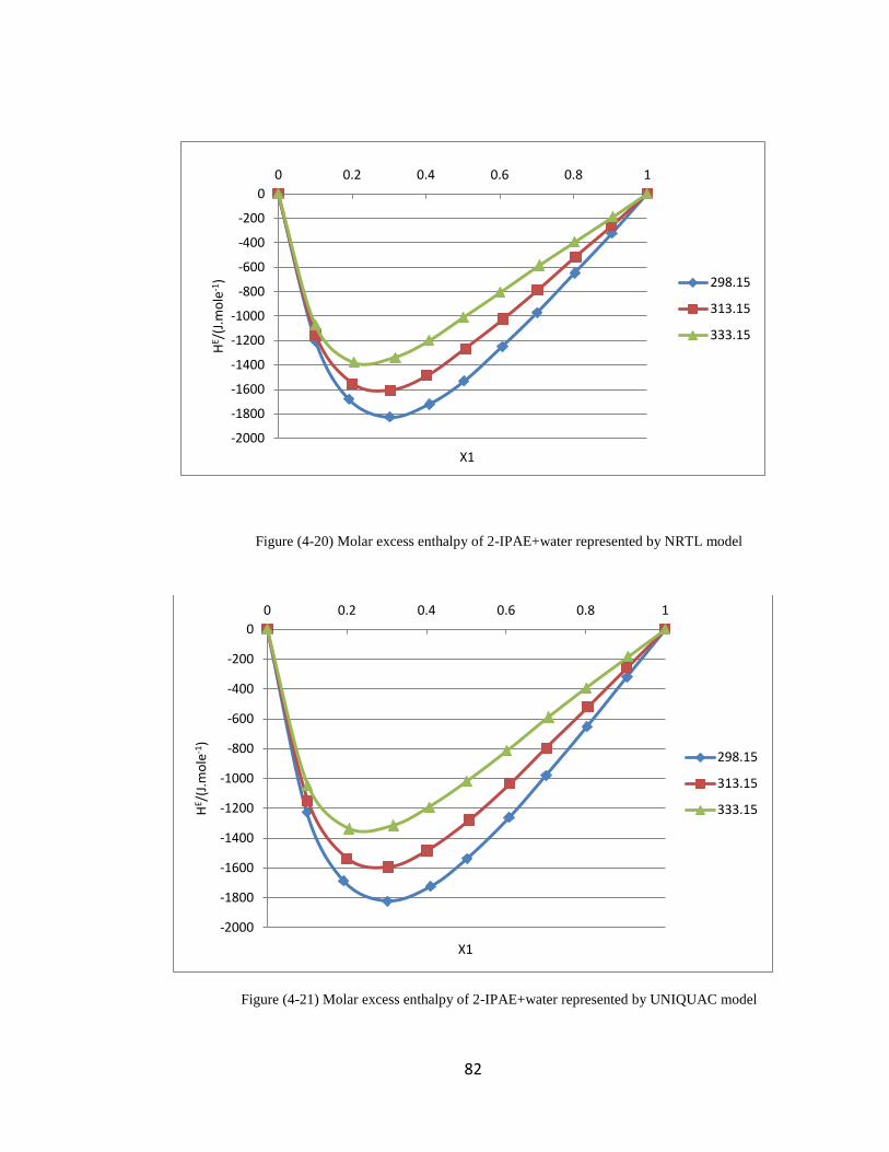
82

Figure (4-20) Molar excess enthalpy of 2-IPAE+water represented by NRTL model

Figure (4-21) Molar excess enthalpy of 2-IPAE+water represented by UNIQUAC model

-2000

-1800

-1600

-1400

-1200

-1000

-800

-600

-400

-200

0

0 0.2 0.4 0.6 0.8 1

HE /

(J.m

ole

-1)

X1

298.15

313.15

333.15

-2000

-1800

-1600

-1400

-1200

-1000

-800

-600

-400

-200

0

0 0.2 0.4 0.6 0.8 1

HE /

(J.m

ole

-1)

X1

298.15

313.15

333.15

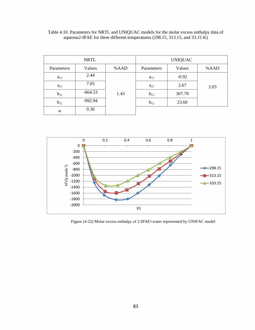
83

Table 4.10. Parameters for NRTL and UNIQUAC models for the molar excess enthalpy data of

aqueous2-IPAE for three different temperatures (298.15, 313.15, and 33.15 K)

NRTL UNIQUAC

Parameters Values %AAD Parameters Values %AAD

a12 2.44

1.43

a12 -0.92

2.03

a21 7.05 a21 2.67

b12 -664.53 b12 307.70

b12 -992.94 b12 23.60

α 0.30

Figure (4-22) Molar excess enthalpy of 2-IPAE+water represented by UNIFAC model

-2000

-1800

-1600

-1400

-1200

-1000

-800

-600

-400

-200

0

0 0.2 0.4 0.6 0.8 1

HE /

(J.m

ole

-1)

X1

298.15

313.15

333.15

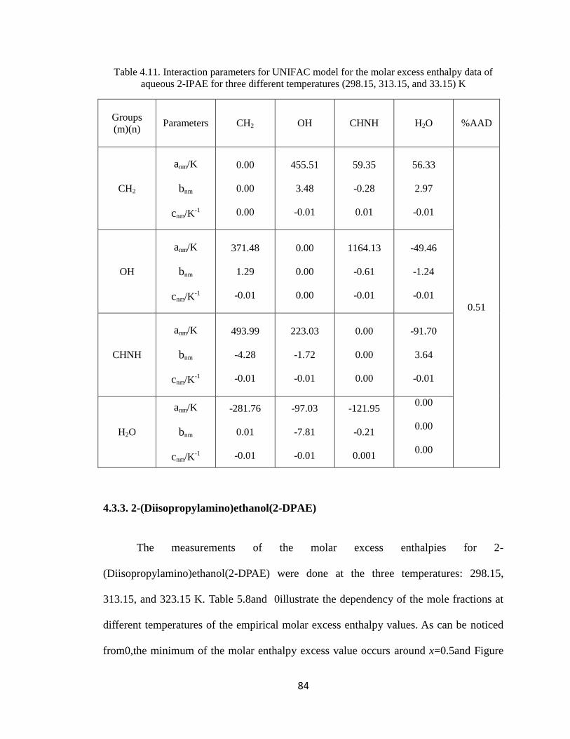
84

Table 4.11. Interaction parameters for UNIFAC model for the molar excess enthalpy data of

aqueous 2-IPAE for three different temperatures (298.15, 313.15, and 33.15) K

Groups

(m)(n)

Parameters CH2 OH CHNH H2O %AAD

CH2

anm/K

bnm

cnm/K-1

0.00

0.00

0.00

455.51

3.48

-0.01

59.35

-0.28

0.01

56.33

2.97

-0.01

0.51

OH

anm/K

bnm

cnm/K-1

371.48

1.29

-0.01

0.00

0.00

0.00

1164.13

-0.61

-0.01

-49.46

-1.24

-0.01

CHNH

anm/K

bnm

cnm/K-1

493.99

-4.28

-0.01

223.03

-1.72

-0.01

0.00

0.00

0.00

-91.70

3.64

-0.01

H2O

anm/K

bnm

cnm/K-1

-281.76

0.01

-0.01

-97.03

-7.81

-0.01

-121.95

-0.21

0.001

0.00

0.00

0.00

4.3.3. 2-(Diisopropylamino)ethanol(2-DPAE)

The measurements of the molar excess enthalpies for 2-

(Diisopropylamino)ethanol(2-DPAE) were done at the three temperatures: 298.15,

313.15, and 323.15 K. Table 5.8and 0illustrate the dependency of the mole fractions at

different temperatures of the empirical molar excess enthalpy values. As can be noticed

from 0,the minimum of the molar enthalpy excess value occurs around x=0.5and Figure

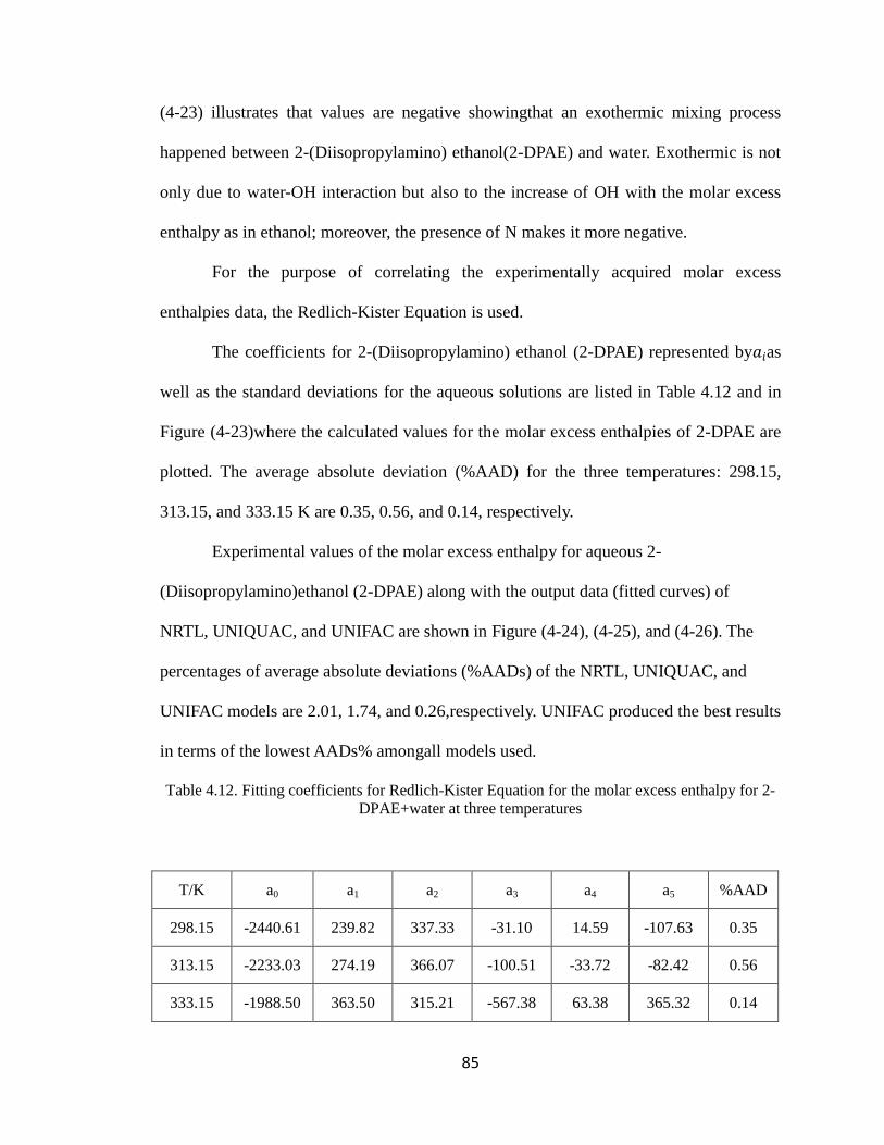
85

(4-23) illustrates that values are negative showingthat an exothermic mixing process

happened between 2-(Diisopropylamino) ethanol(2-DPAE) and water. Exothermic is not

only due to water-OH interaction but also to the increase of OH with the molar excess

enthalpy as in ethanol; moreover, the presence of N makes it more negative.

For the purpose of correlating the experimentally acquired molar excess

enthalpies data, the Redlich-Kister Equation is used.

The coefficients for 2-(Diisopropylamino) ethanol (2-DPAE) represented by as

well as the standard deviations for the aqueous solutions are listed in Table 4.12 and in

Figure (4-23)where the calculated values for the molar excess enthalpies of 2-DPAE are

plotted. The average absolute deviation (%AAD) for the three temperatures: 298.15,

313.15, and 333.15 K are 0.35, 0.56, and 0.14, respectively.

Experimental values of the molar excess enthalpy for aqueous 2-

(Diisopropylamino)ethanol (2-DPAE) along with the output data (fitted curves) of

NRTL, UNIQUAC, and UNIFAC are shown in Figure (4-24), (4-25), and (4-26). The

percentages of average absolute deviations (%AADs) of the NRTL, UNIQUAC, and

UNIFAC models are 2.01, 1.74, and 0.26,respectively. UNIFAC produced the best results

in terms of the lowest AADs% amongall models used.

Table 4.12. Fitting coefficients for Redlich-Kister Equation for the molar excess enthalpy for 2-

DPAE+water at three temperatures

T/K a0 a1 a2 a3 a4 a5 %AAD

298.15 -2440.61 239.82 337.33 -31.10 14.59 -107.63 0.35

313.15 -2233.03 274.19 366.07 -100.51 -33.72 -82.42 0.56

333.15 -1988.50 363.50 315.21 -567.38 63.38 365.32 0.14

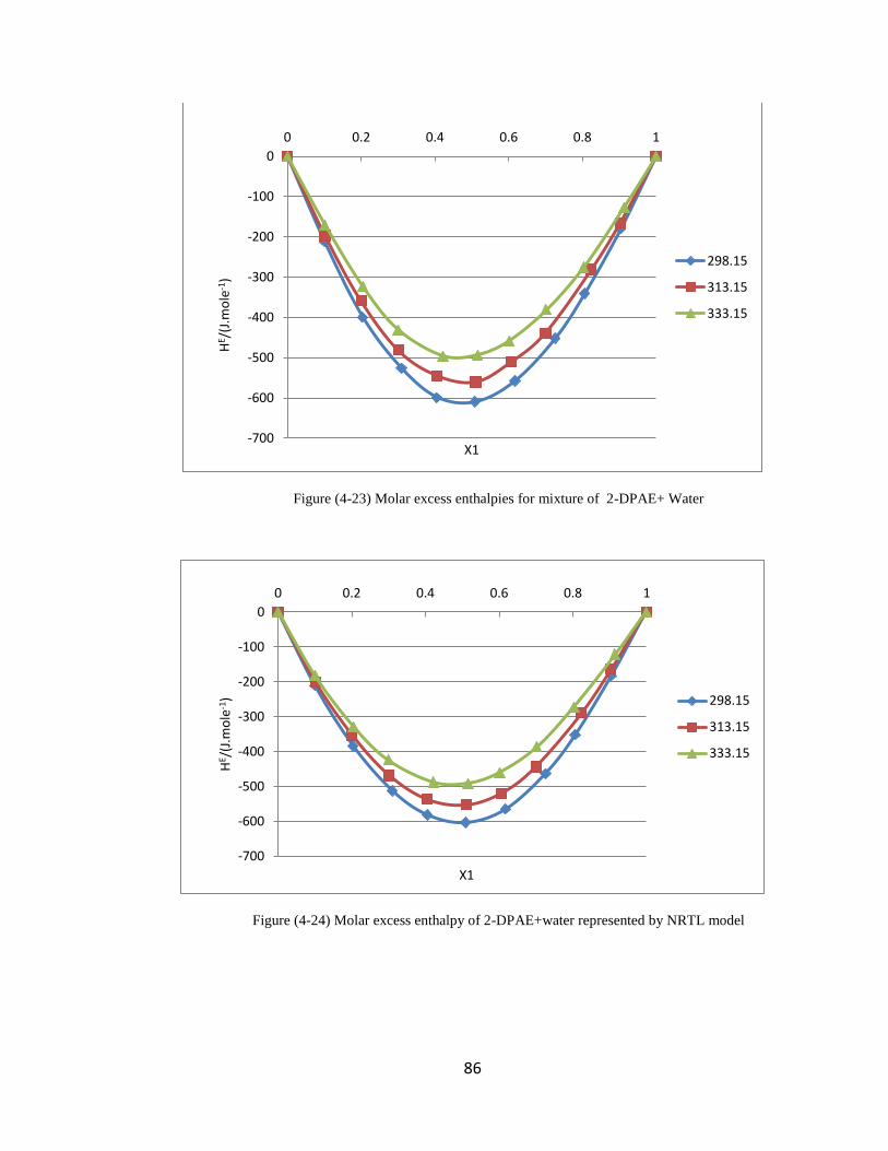
86

Figure (4-23) Molar excess enthalpies for mixture of 2-DPAE+ Water

Figure (4-24) Molar excess enthalpy of 2-DPAE+water represented by NRTL model

-700

-600

-500

-400

-300

-200

-100

0

0 0.2 0.4 0.6 0.8 1

HE /

(J.m

ole

-1)

X1

298.15

313.15

333.15

-700

-600

-500

-400

-300

-200

-100

0

0 0.2 0.4 0.6 0.8 1

HE /

(J.m

ole

-1)

X1

298.15

313.15

333.15

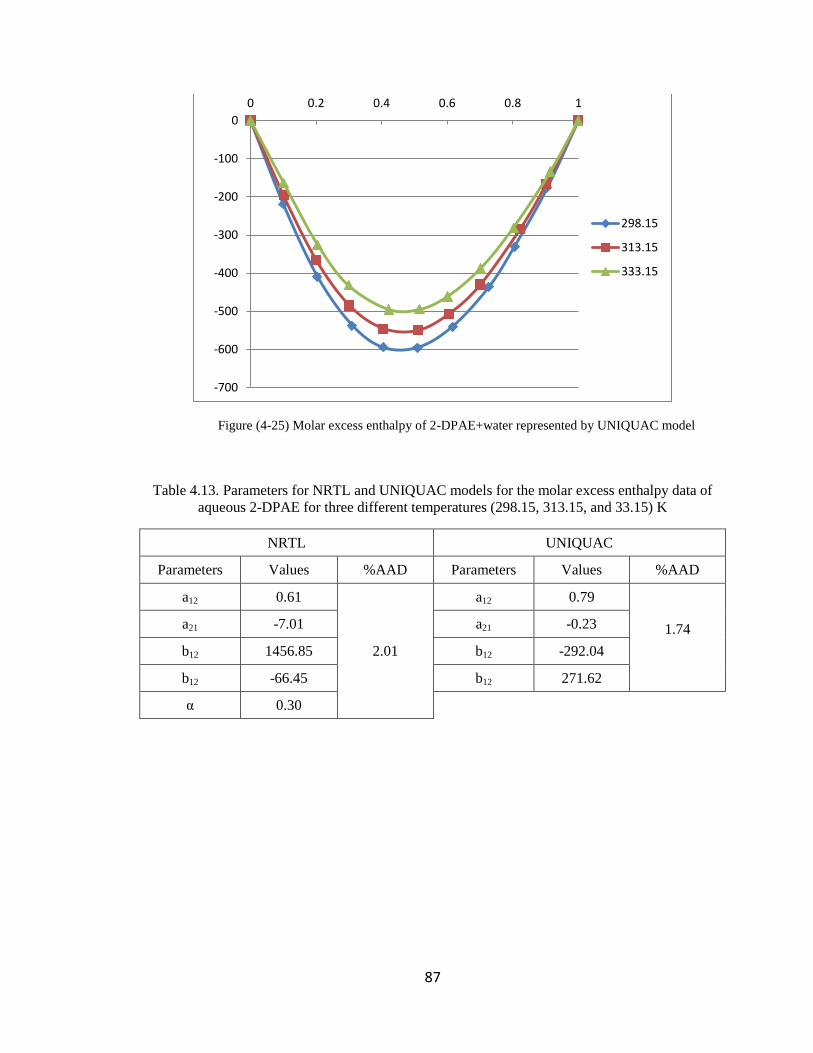
87

Figure (4-25) Molar excess enthalpy of 2-DPAE+water represented by UNIQUAC model

Table 4.13. Parameters for NRTL and UNIQUAC models for the molar excess enthalpy data of

aqueous 2-DPAE for three different temperatures (298.15, 313.15, and 33.15) K

NRTL UNIQUAC

Parameters Values %AAD Parameters Values %AAD

a12 0.61

2.01

a12 0.79

1.74

a21 -7.01 a21 -0.23

b12 1456.85 b12 -292.04

b12 -66.45 b12 271.62

α 0.30

-700

-600

-500

-400

-300

-200

-100

0

0 0.2 0.4 0.6 0.8 1

298.15

313.15

333.15

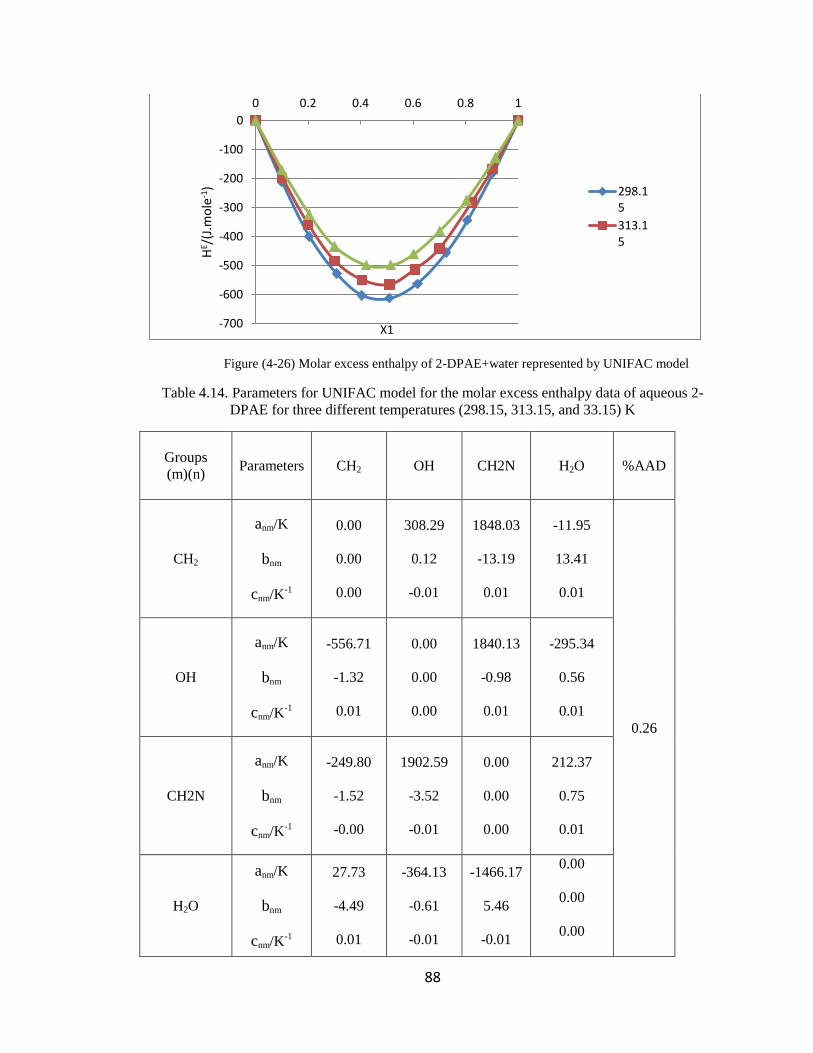
88

Figure (4-26) Molar excess enthalpy of 2-DPAE+water represented by UNIFAC model

Table 4.14. Parameters for UNIFAC model for the molar excess enthalpy data of aqueous 2-

DPAE for three different temperatures (298.15, 313.15, and 33.15) K

Groups

(m)(n)

Parameters CH2 OH CH2N H2O %AAD

CH2

anm/K

bnm

cnm/K-1

0.00

0.00

0.00

308.29

0.12

-0.01

1848.03

-13.19

0.01

-11.95

13.41

0.01

0.26

OH

anm/K

bnm

cnm/K-1

-556.71

-1.32

0.01

0.00

0.00

0.00

1840.13

-0.98

0.01

-295.34

0.56

0.01

CH2N

anm/K

bnm

cnm/K-1

-249.80

-1.52

-0.00

1902.59

-3.52

-0.01

0.00

0.00

0.00

212.37

0.75

0.01

H2O

anm/K

bnm

cnm/K-1

27.73

-4.49

0.01

-364.13

-0.61

-0.01

-1466.17

5.46

-0.01

0.00

0.00

0.00

-700

-600

-500

-400

-300

-200

-100

0

0 0.2 0.4 0.6 0.8 1

HE /

(J.m

ole

-1)

X1

298.15

313.15

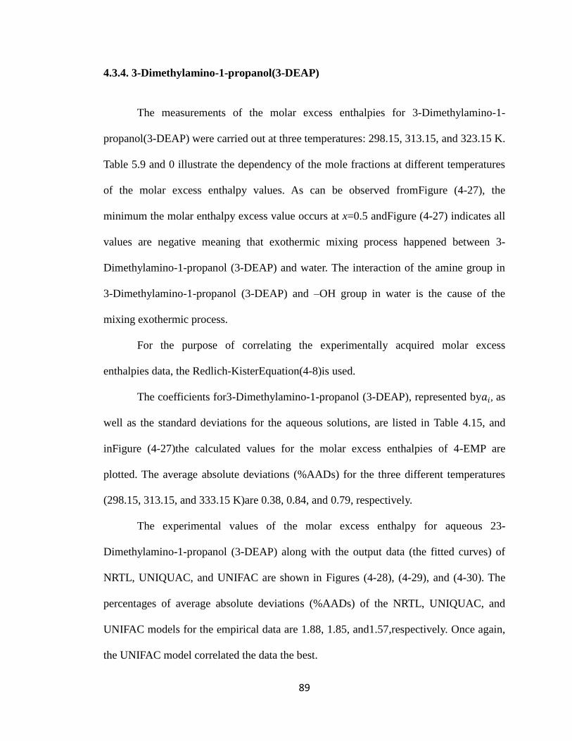
89

4.3.4. 3-Dimethylamino-1-propanol(3-DEAP)

The measurements of the molar excess enthalpies for 3-Dimethylamino-1-

propanol(3-DEAP) were carried out at three temperatures: 298.15, 313.15, and 323.15 K.

Table 5.9 and 0 illustrate the dependency of the mole fractions at different temperatures

of the molar excess enthalpy values. As can be observed fromFigure (4-27), the

minimum the molar enthalpy excess value occurs at x=0.5 andFigure (4-27) indicates all

values are negative meaning that exothermic mixing process happened between 3-

Dimethylamino-1-propanol (3-DEAP) and water. The interaction of the amine group in

3-Dimethylamino-1-propanol (3-DEAP) and –OH group in water is the cause of the

mixing exothermic process.

For the purpose of correlating the experimentally acquired molar excess

enthalpies data, the Redlich-KisterEquation (4-8)is used.

The coefficients for3-Dimethylamino-1-propanol (3-DEAP), represented by , as

well as the standard deviations for the aqueous solutions, are listed in Table 4.15, and

inFigure (4-27)the calculated values for the molar excess enthalpies of 4-EMP are

plotted. The average absolute deviations (%AADs) for the three different temperatures

(298.15, 313.15, and 333.15 K)are 0.38, 0.84, and 0.79, respectively.

The experimental values of the molar excess enthalpy for aqueous 23-

Dimethylamino-1-propanol (3-DEAP) along with the output data (the fitted curves) of

NRTL, UNIQUAC, and UNIFAC are shown in Figures (4-28), (4-29), and (4-30). The

percentages of average absolute deviations (%AADs) of the NRTL, UNIQUAC, and

UNIFAC models for the empirical data are 1.88, 1.85, and1.57,respectively. Once again,

the UNIFAC model correlated the data the best.

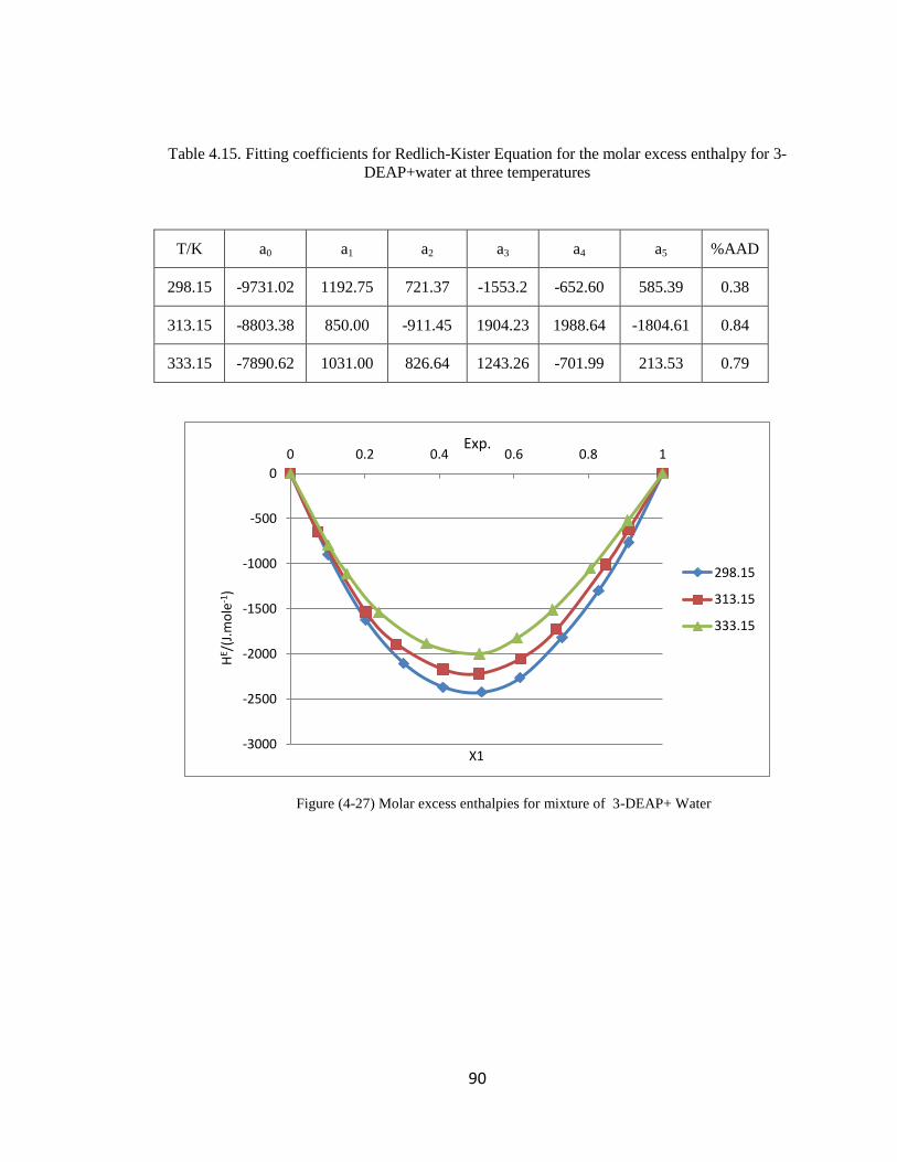
90

Table 4.15. Fitting coefficients for Redlich-Kister Equation for the molar excess enthalpy for 3-

DEAP+water at three temperatures

T/K a0 a1 a2 a3 a4 a5 %AAD

298.15 -9731.02 1192.75 721.37 -1553.2 -652.60 585.39 0.38

313.15 -8803.38 850.00 -911.45 1904.23 1988.64 -1804.61 0.84

333.15 -7890.62 1031.00 826.64 1243.26 -701.99 213.53 0.79

Figure (4-27) Molar excess enthalpies for mixture of 3-DEAP+ Water

-3000

-2500

-2000

-1500

-1000

-500

0

0 0.2 0.4 0.6 0.8 1

HE /

(J.m

ole

-1)

X1

Exp.

298.15

313.15

333.15

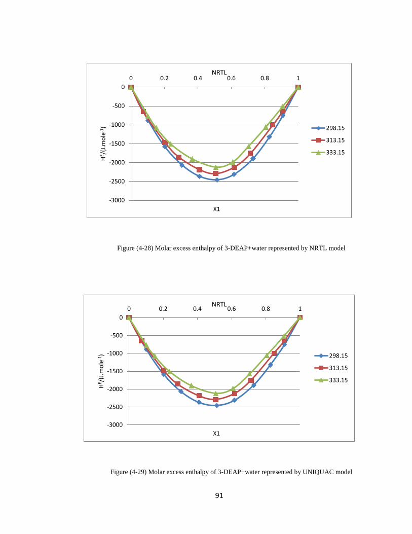
91

Figure (4-28) Molar excess enthalpy of 3-DEAP+water represented by NRTL model

Figure (4-29) Molar excess enthalpy of 3-DEAP+water represented by UNIQUAC model

-3000

-2500

-2000

-1500

-1000

-500

0

0 0.2 0.4 0.6 0.8 1

HE /

(J.m

ole

-1)

X1

NRTL

298.15

313.15

333.15

-3000

-2500

-2000

-1500

-1000

-500

0

0 0.2 0.4 0.6 0.8 1

HE /

(J.m

ole

-1)

X1

NRTL

298.15

313.15

333.15

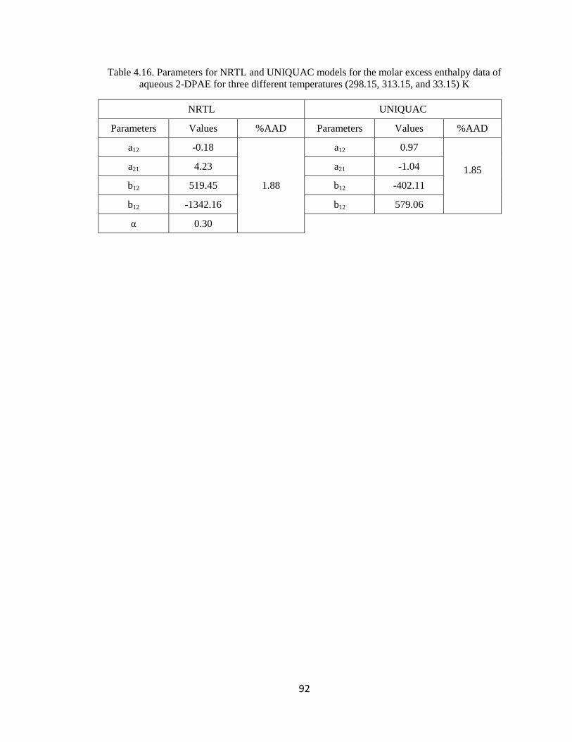
92

Table 4.16. Parameters for NRTL and UNIQUAC models for the molar excess enthalpy data of

aqueous 2-DPAE for three different temperatures (298.15, 313.15, and 33.15) K

NRTL UNIQUAC

Parameters Values %AAD Parameters Values %AAD

a12 -0.18

1.88

a12 0.97

1.85

a21 4.23 a21 -1.04

b12 519.45 b12 -402.11

b12 -1342.16 b12 579.06

α 0.30

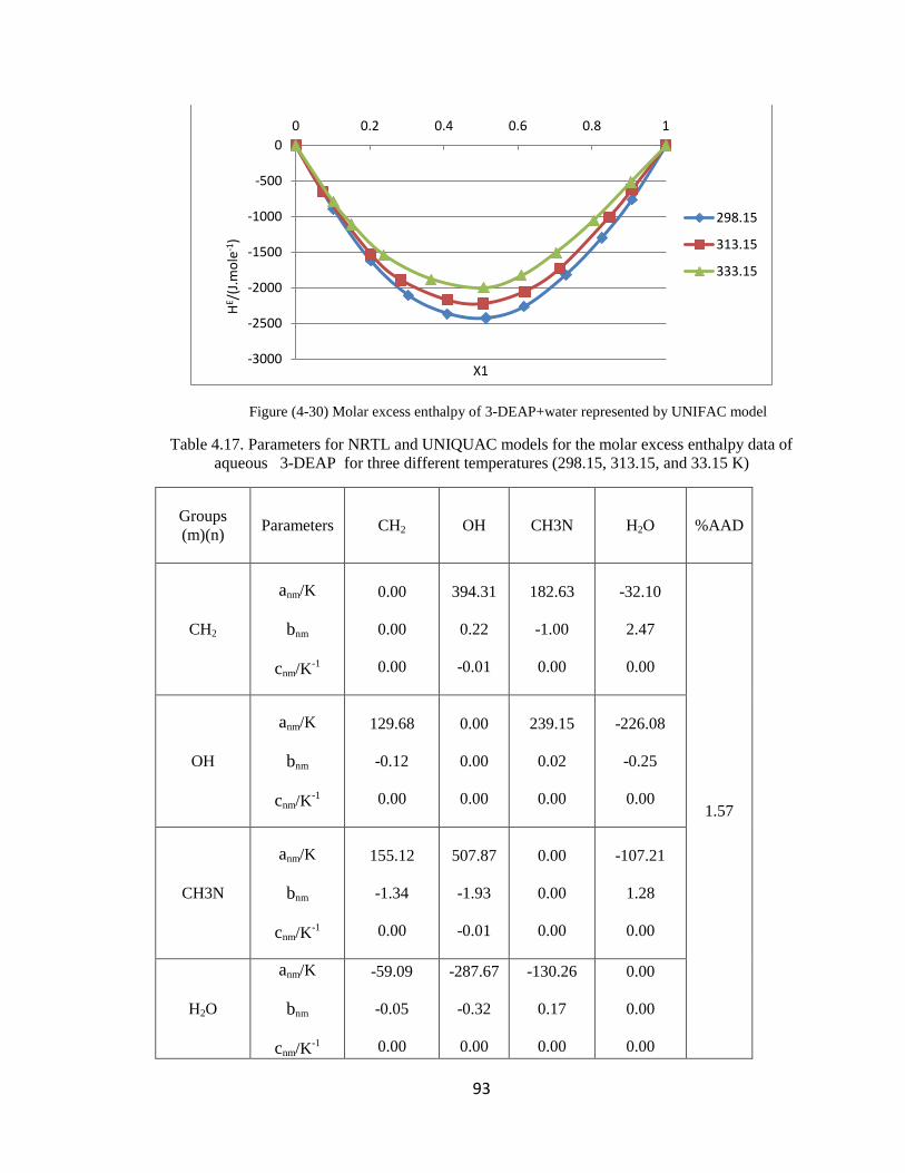
93

Figure (4-30) Molar excess enthalpy of 3-DEAP+water represented by UNIFAC model

Table 4.17. Parameters for NRTL and UNIQUAC models for the molar excess enthalpy data of

aqueous 3-DEAP for three different temperatures (298.15, 313.15, and 33.15 K)

Groups

(m)(n)

Parameters CH2 OH CH3N H2O %AAD

CH2

anm/K

bnm

cnm/K-1

0.00

0.00

0.00

394.31

0.22

-0.01

182.63

-1.00

0.00

-32.10

2.47

0.00

1.57

OH

anm/K

bnm

cnm/K-1

129.68

-0.12

0.00

0.00

0.00

0.00

239.15

0.02

0.00

-226.08

-0.25

0.00

CH3N

anm/K

bnm

cnm/K-1

155.12

-1.34

0.00

507.87

-1.93

-0.01

0.00

0.00

0.00

-107.21

1.28

0.00

H2O

anm/K

bnm

cnm/K-1

-59.09

-0.05

0.00

-287.67

-0.32

0.00

-130.26

0.17

0.00

0.00

0.00

0.00

-3000

-2500

-2000

-1500

-1000

-500

0

0 0.2 0.4 0.6 0.8 1

HE /

(J.m

ole

-1)

X1

298.15

313.15

333.15

94

4.3.5. 1-Dimethylamino-2-propanol (1-DEAP)

The measurements of the molar excess enthalpies for 1-Dimethylamino-2-

propanol (1-DEAP) were performed at three temperatures: 298.15, 313.15, and 323.15

K. Table 5.10and Figure (4-31) illustrate the dependency of the mole fractions at

different temperatures for the molar excess enthalpy values. As can be noticed from 0,

the minimum molar enthalpy excess value occurs near x=0.4 andFigure (4-31)shows that

values are negative and that themixing process between 1-Dimethylamino-2-propanol (1-

DEAP) and water was exothermic.

For the purpose of correlating the experimentally acquired molar excess

enthalpies data, the Redlich-Kister Equation is used.

The coefficients for in 1-Dimethylamino-2-propanol (1-DEAP) which are

represented by as well as the standard deviations for the aqueous solutions are listed in

Table 4.18, and plotted in Figure (4-31). The average absolute deviations (%AADs) for

the three different temperatures (298.15, 313.15, and 333.15 K)are 0.49, 0.25 and 0.85,

respectively.

The experimental values of the molar excess enthalpy for aqueous 1-

Dimethylamino-2-propanol (1-DEAP) along with the output data (fitted curves) of

NRTL, UNIQUAC, and UNIFAC are shown inFigure (4-32), (4-33), and (4-34). The

percentages of average absolute deviations (%AADs) of NRTL, UNIQUAC, and

UNIFAC models for the empirical data are 1.04, 1.13, and0.97, respectively. UNIFAC

was the best model in terms of correlating the data among all other models used.

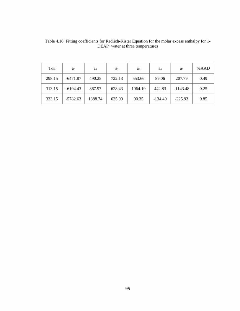
95

Table 4.18. Fitting coefficients for Redlich-Kister Equation for the molar excess enthalpy for 1-

DEAP+water at three temperatures

T/K a0 a1 a2 a3 a4 a5 %AAD

298.15 -6471.87 490.25 722.13 553.66 89.06 207.79 0.49

313.15 -6194.43 867.97 628.43 1064.19 442.83 -1143.48 0.25

333.15 -5782.63 1388.74 625.99 90.35 -134.40 -225.93 0.85

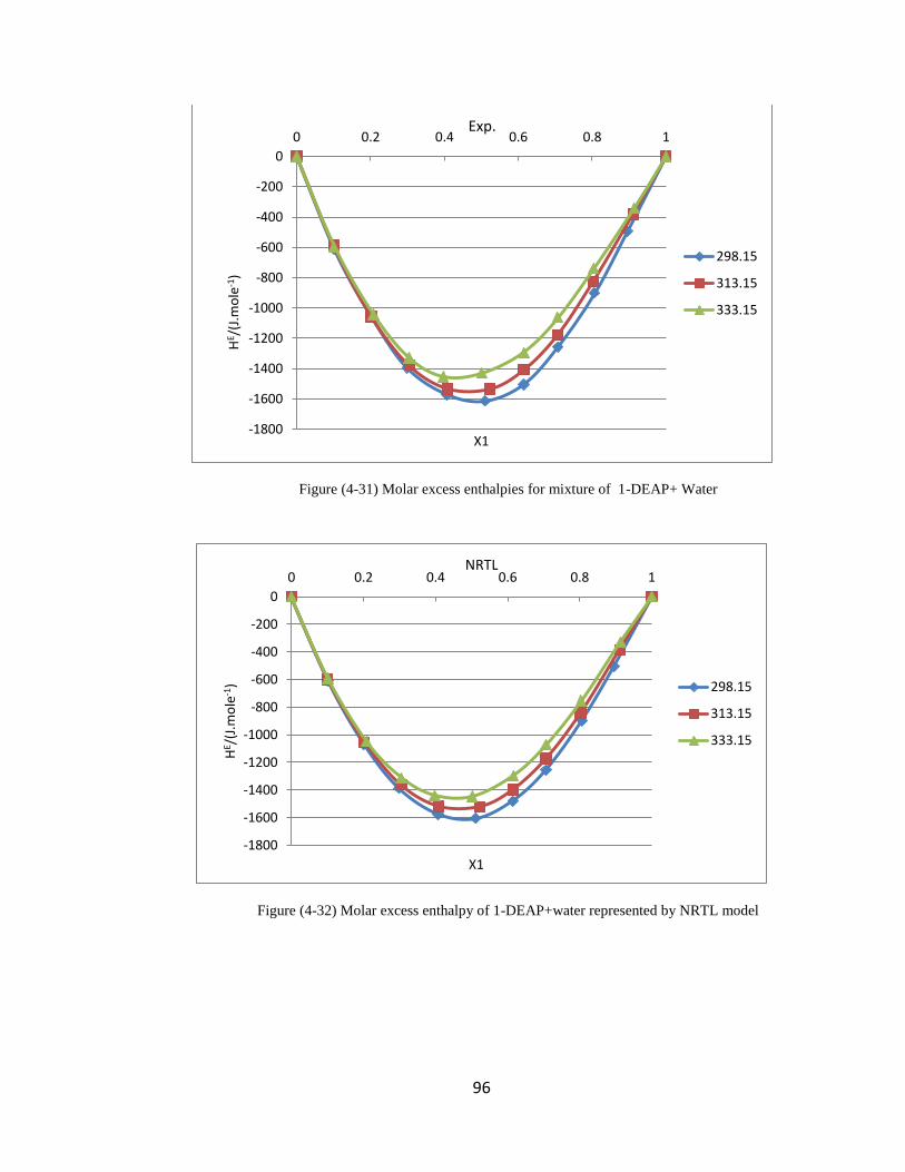
96

Figure (4-31) Molar excess enthalpies for mixture of 1-DEAP+ Water

Figure (4-32) Molar excess enthalpy of 1-DEAP+water represented by NRTL model

-1800

-1600

-1400

-1200

-1000

-800

-600

-400

-200

0

0 0.2 0.4 0.6 0.8 1

HE /

(J.m

ole

-1)

X1

Exp.

298.15

313.15

333.15

-1800

-1600

-1400

-1200

-1000

-800

-600

-400

-200

0

0 0.2 0.4 0.6 0.8 1

HE /

(J.m

ole

-1)

X1

NRTL

298.15

313.15

333.15

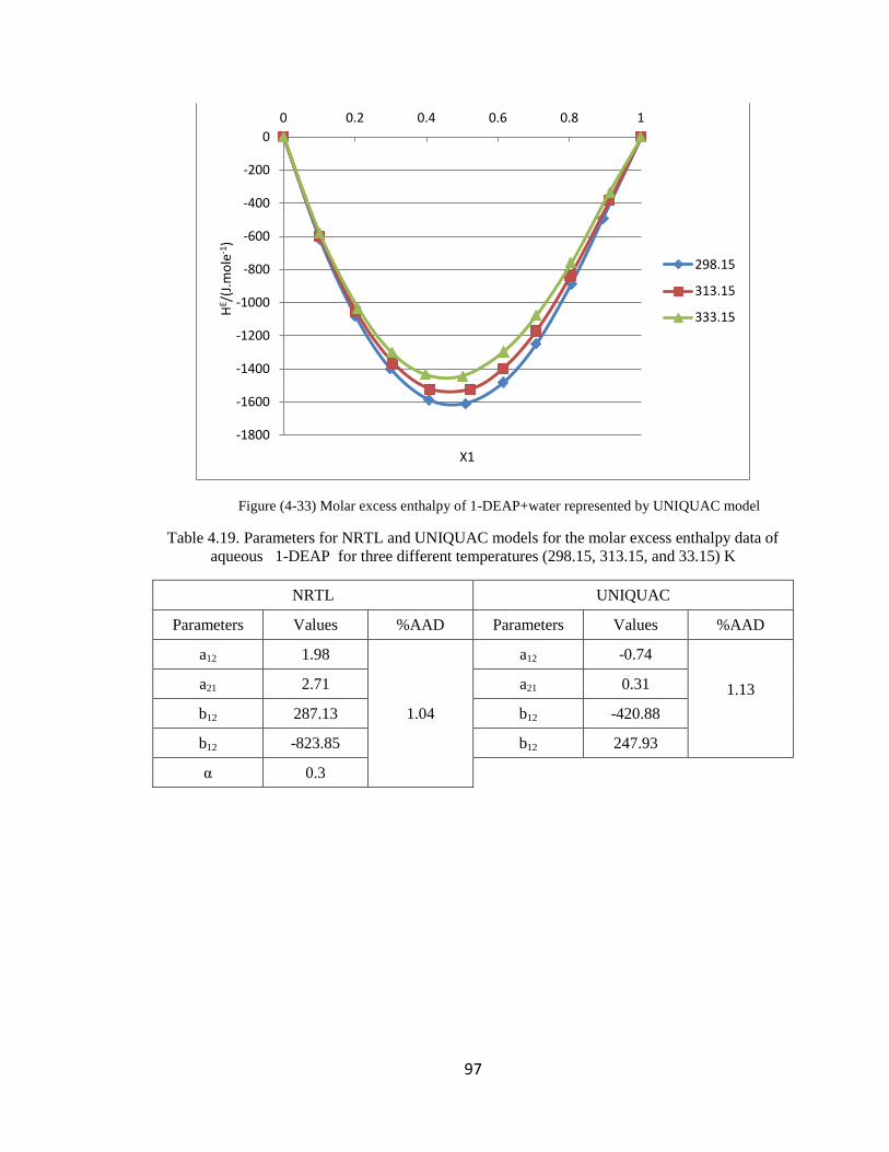
97

Figure (4-33) Molar excess enthalpy of 1-DEAP+water represented by UNIQUAC model

Table 4.19. Parameters for NRTL and UNIQUAC models for the molar excess enthalpy data of

aqueous 1-DEAP for three different temperatures (298.15, 313.15, and 33.15) K

NRTL UNIQUAC

Parameters Values %AAD Parameters Values %AAD

a12 1.98

1.04

a12 -0.74

1.13

a21 2.71 a21 0.31

b12 287.13 b12 -420.88

b12 -823.85 b12 247.93

α 0.3

-1800

-1600

-1400

-1200

-1000

-800

-600

-400

-200

0

0 0.2 0.4 0.6 0.8 1

HE /

(J.m

ole

-1)

X1

298.15

313.15

333.15

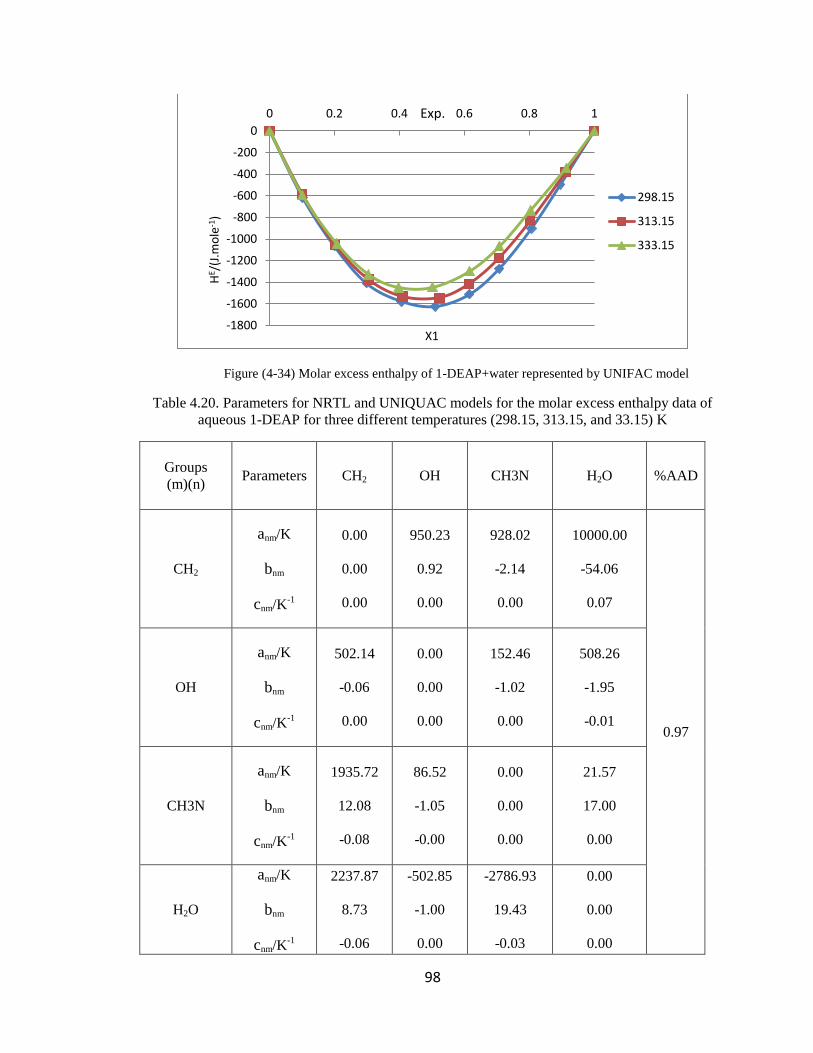
98

Figure (4-34) Molar excess enthalpy of 1-DEAP+water represented by UNIFAC model

Table 4.20. Parameters for NRTL and UNIQUAC models for the molar excess enthalpy data of

aqueous 1-DEAP for three different temperatures (298.15, 313.15, and 33.15) K

Groups

(m)(n)

Parameters CH2 OH CH3N H2O %AAD

CH2

anm/K

bnm

cnm/K-1

0.00

0.00

0.00

950.23

0.92

0.00

928.02

-2.14

0.00

10000.00

-54.06

0.07

0.97

OH

anm/K

bnm

cnm/K-1

502.14

-0.06

0.00

0.00

0.00

0.00

152.46

-1.02

0.00

508.26

-1.95

-0.01

CH3N

anm/K

bnm

cnm/K-1

1935.72

12.08

-0.08

86.52

-1.05

-0.00

0.00

0.00

0.00

21.57

17.00

0.00

H2O

anm/K

bnm

cnm/K-1

2237.87

8.73

-0.06

-502.85

-1.00

0.00

-2786.93

19.43

-0.03

0.00

0.00

0.00

-1800

-1600

-1400

-1200

-1000

-800

-600

-400

-200

0

0 0.2 0.4 0.6 0.8 1

HE /

(J.m

ole

-1)

X1

Exp.

298.15

313.15

333.15

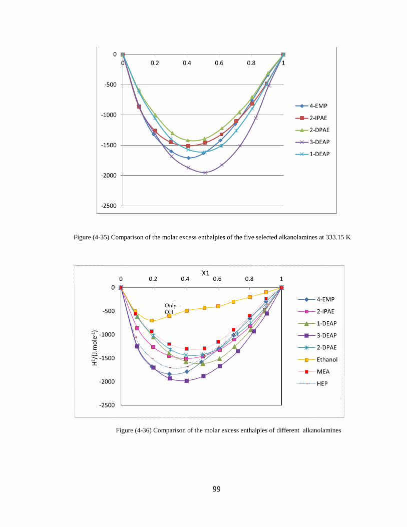
99

Figure (4-35) Comparison of the molar excess enthalpies of the five selected alkanolamines at 333.15 K

Figure (4-36) Comparison of the molar excess enthalpies of different alkanolamines

-2500

-2000

-1500

-1000

-500

0

0 0.2 0.4 0.6 0.8 1

4-EMP

2-IPAE

2-DPAE

3-DEAP

1-DEAP

-2500

-2000

-1500

-1000

-500

0

0 0.2 0.4 0.6 0.8 1

HE /

(J.m

ole

-1)

X1

4-EMP

2-IPAE

1-DEAP

3-DEAP

2-DPAE

Ethanol

MEA

HEP

Only -OH

100

CHAPTER 5: CONCLUSION

Molar heat capacities for the five selected aqueous alkanolamine solutions 4-

EMP (C6H13NO), 2-IPAE (C5H13NO), 2-DPAE (C8H19NO), 3-DEAP (C5H13NO),

and 1-DEAP (C5H13NO) at the temperature from 298.15 to 353.15 K were measured for

the entire mole fractions; in addition, the molar excess heat capacity values were derived

from the experimental values of Cp.In order to correlate the data, the Redlich-Kister

Equation was used. Among the five selected alkanolamines solutions, the solvent with

the highest value of molar heat capacity was2-DPAE, whereas 4-EMP possessed the

lowest value. This study confirmsthat the values of molar heat capacities are dominated

by group contributions of –CH2 and the effect of these group contributions become

greater as temperature increases. In the present study, it can be concluded that 2-DPAE

has the largest value of molar heat capacity due to the larger number of –CH3 groups

followed by 1-DEAP. According to the literature review, the role of –NH group is

important, Therefore, possession of a –NH group by 2-IPAE gives this alkanolamine

third place in terms of molar heat capacity value among the rest of the alkanolamines.

For the remaining selected alkanolamines, 3-DEAP has a lower value of molar heat

capacity compared to 2-DPAE, 1-DEAP, and 2-IPAE. Figure (4-15) shows 2-IPAE has

higher value of molar heat capacity compared to 3-DEAP whereas both have the same

number of –CH3. This comparison shows the role of –NH group contribution.

Eventually 4-EMP has the smallest value of molar heat capacity due to less contribution

of –CH3 and –NH groups in 4-Ethylmorpholine.

Molar excess enthalpies were measured for the five selected aqueous

alkanolamine solutions 4-EMP, 2-IPAE, 2-DPAE, 3-DEAP, and 1-DEAP at the three

101

different temperatures (298.15, 313.15, and 333.15 K) for the entire mole fractions.

The obtained experimental values were correlated as a function of mole fractions

using the Redlich-Kister Equation. Two solutions theory models (NRTL and

UNIQUAC), as well as a group contribution model: Modified UNIFAC (Dortmund)

were used.

Among the three models, the modified UNIFAC (Dortmund) correlated the data

with the lowest AAD % in all cases.

Comparison between the five selected alkanolamines shows that 3-DEAP

exhibited the highest values of molar excess enthalpies on the negative side compared to

the other selected alkanolamines, while2-DPAE displayed the smallest negative values of

molar excess enthalpies. A comparison between the two amines proves the significant

role of steric hindrance effects. In 2-(Diisopropylamino) ethanol, nitrogen atom is

surrounded by –CH3 groups and provides less access to the water molecules, therefore,

the nitrogen atom has less tendency to interact with water. On the other side , nitrogen

atom in 3-Dimethylamino-1-propanol has more access to water molecules and due to

more accessibility, the interaction between nitrogen atom and water molecules liberates

more energy, consequently produces larger amount of molar excess enthalpy and since

exothermic process happens, molar excess enthalpy increases in the negative side.

Another comparison between 3-Dimethylamino-1-propanol and 1-Dimethylamino-2-

propanol shows the value of molar excess enthalpies depends on the position of –OH. It

also can be concluded that the interaction between water hydrogen and –N group is more

dominant than the interactions between –OH and the water hydrogen. This study

provides new calorimetric data of five aqueous alkanolamines which in conjunction with

other information such as CO2 solubility and kinetic, data may be useful to judge the

102

potential of theses amines for CO2 capturing. We therefore highly recommend measuring

the kinetics of CO2 in aqueous 3-DEAP.

103

REFERENCES

Abrams, Denis S., and John M. Prausnitz. "Statistical thermodynamics of liquid mixtures: a

new expression for the excess Gibbs energy of partly or completely miscible systems."

AIChE Journal 21/1 (1975): 116-128.

Alonso R., GuerreroR., Corrales J.A. “Excess Molar Enthalpies of

(Methylcyclohexane+Alkanol) at 323K. Results for n-Butanol, n-Pentanol, and n-

Hexanol”, Elsevier.

Anderson, T. F., and J. M. Prausnitz."Application of the UNIQUAC Equation to

calculation of multicomponent phase equilibria.1. Vapor-liquid equilibria." Industrial

& Engineering Chemistry Process Design and Development 17/4 (1978): 552-561.

Becker, Lars, and Jürgen Gmehling."Measurement of heat capacities for 12 organic

substances by Tian-Calvetcalorimetry." Journal of Chemical & Engineering Data 46/6

(2001): 1638-1642.

Bet Metz, Ogunlade Davidson, Heleen de Coninck, Manuela Loos and Leo Meyer(Eds.).,

“IPCC”, 2005.

Bevington, Philip R., and D. Keith Robinson.Data reduction and error analysis for the

physical sciences.Vol. 2. New York: McGraw-Hill, 1969.

Calvet, Edouard, and Henri Prat.Recent progress in microcalorimetry. Ed. H. A. Skinner.

Oxford: Pergamon Press, 1963.

104

Chen, Yan-Jen, Tzn-Wei Shih, and Meng-Hui Li. "Heat capacity of aqueous mixtures of

monoethanolamine with N-methyldiethanolamine." Journal of Chemical &

Engineering Data 46/1 (2001): 51-55.

Chiu, Li-Feng, Hsiao-Fen Liu, and Meng-Hui Li. "Heat capacity of alkanolamines by

differential scanning calorimetry." Journal of Chemical & Engineering Data 44/3

(1999): 631-636.

Czichos, Horst, Tetsuya Saito, and Leslie Smith, eds. Springer handbook of materials

measurement methods.Springerverlag Berlin Heidelberg, 2006.

Daniel C., Harris, Quantitative chemical analysis. W. H. Freeman, 2010.

Desnoyers, Jacques E., and GéraldPerron."Treatment of excess thermodynamic quantities

for liquid mixtures." Journal of Solution Chemistry 26/8 (1997): 749-755.

Fanni, Anna Maria, et al. "DISQUAC predictions of excess enthalpies of the ternary

mixture: tetrahydrofuran+ cyclohexane+ butanenitrile." Fluid phase equilibria 126/2

(1996): 163-175.

Fredenslund, Aage, Jürgen Gmehling, and Peter Rasmussen.“Vapor-liquid equilibria using

UNIFAC: a group-contribution method”. Vol. 1. Amsterdam: Elsevier, 1977.

Fredenslund, Aage, Russell L. Jones, and John M. Prausnitz."Group‐contribution

estimation of activity coefficients in nonideal liquid mixtures."AIChE Journal 21/6

(1975): 1086-1099.

Gmehling, Juergen, and Peter Rasmussen. "Flash points of flammable liquid mixtures using

UNIFAC" Industrial & Engineering Chemistry Fundamentals 21/2 (1982): 186-188.

105

Gmehling, Jürgen G., Thomas F. Anderson, and John M. Prausnitz."Solid-liquid equilibria

using UNIFAC." Industrial & Engineering Chemistry Fundamentals 17/4 (1978): 269-

273.

Goodwin, Anthony, K. N. Marsh, and W. A. Wakeham. Measurement of the

thermodynamic properties of single phases.Vol. 6. Elsevier Science, 2003.

Gottlieb, Moshe, and MordechayHerskowitz."Estimation of the η parameter for poly

(dimethylsiloxane) solutions by the UNIFAC group contribution method."

Macromolecules 14/5 (1981): 1468-1471.

Gow, Arthur S. "Calculation of vapor-liquid equilibria from infinite-dilution excess

enthalpy data using the Wilson or NRTL Equation." Industrial &Engineering

Chemistry Research 32/12 (1993): 3150-3161.

Guggenheim, Edward A. Mixtures: the theory of the equilibrium properties of some simple

classes of mixtures, solutions and alloys. Clarendon Press, 1952.

Hanks, Richard W., Romeo L. Tan, and James J. Christensen."Limits on the simultaneous

correlation ofdata by the NRTL, LEMF and Wilson's Equations."ThermochimicaActa

23/1 (1978): 41-55.

Hanks, Richard W., Romeo L. Tan, and James J. Christensen. "The prediction of high

temperature vapor—liquid equilbiria from lower temperature heat of mixing data."

ThermochimicaActa 27/1 (1978): 9-18.

Health-based reassessment of administrative occupational exposure limits, Committee of

the Health Council of the Netherlands.

106

Henni, Amr, Juelin Li, and PaitoonTontiwachwuthikul."Reaction kinetics of CO2 in

aqueous ethylenediamine, ethyl ethanolamine, and diethyl monoethanolamine

solutions in the temperature range of 298-313 K, using the stopped-flow technique."

Industrial &Engineering Chemistry Research 46/13 (2007): 4426-4434.

Henni, Amr, Juelin Li, and PaitoonTontiwachwuthikul."Reaction kinetics of CO2 in

aqueous 1-amino-2-propanol, 3-amino-1-propanol, and dimethylmonoethanolamine

solutions in the temperature range of 298-313 K using the stopped-flow technique."

Industrial & Engineering Chemistry Research 47/7 (2008): 2213-2220.

Henni, Amr, et al. "Densities and viscosities for binary mixtures of N-

methyldiethanolamine+ triethylene glycol monomethyl ether from 25° C to 70° C and

N-methyldiethanolamine+ ethanol mixtures at 40° C." Journal of Chemical &

Engineering Data 45/2 (2000): 247-253.

Jensen, Torben, AageFredenslund, and Peter Rasmussen. "Pure-component vapor pressures

using UNIFAC group contribution." Industrial & Engineering Chemistry

Fundamentals 20/3 (1981): 239-246.

Kehiaian, H. V., J. P. E. Grolier, and G. C. Benson."Thermodynamics of organic

mixtures.A generalized quasichemical theory in terms of group surface interactions."

J. Chem. Phys 75/11-12 (1978): 1031-1048.

Lee, Seungmoon, et al. "Physical properties of aqueous sodium glycinate solution as an

absorbent for carbon dioxide removal." Journal of Chemical & Engineering Data 50/5

(2005): 1773-1776.

107

Lim, Kyung-Hee, Wallace B. Whiting, and Duane H. Smith. "Excess enthalpies and liquid-

liquid equilibrium phase compositions of the nonionicamphiphile 2-butoxyethanol and

water." Journal of Chemical and Engineering Data 39/2 (1994): 399-403.

Magnussen, Thomas, Peter Rasmussen, and AageFredenslund."UNIFAC parameter table

for prediction of liquid-liquid equilibrium." Industrial & Engineering Chemistry

Process Design and Development 20/2 (1981): 331-339.

Maham, Y, Hepler, LorenG., et al. "Molar heat capacities of alkanolamines from 299.1 to

397.8 K." Journal of the Chemical Society, Faraday Transactions 93/9 (1997): 1747-

1750.

Maham, Yadollah, Alan E. Mather, and Loren G. Hepler."Excess molar enthalpies of

(water+ alkanolamine) systems and some thermodynamic calculations." Journal of

Chemical & Engineering Data 42/5 (1997): 988-992.

Marongiu, Bruno. "DISQUAC predictions on excess enthalpies of the ternary mixture:

cyclohexane+ propanone+ tetrahydrofuran." Fluid Phase Equilibria 109/1 (1995): 67-

81.

McGlashan, Maxwell Len, and H. F. Stoeckli. "A flow calorimeter for enthalpies of mixing

The enthalpy of mixing ofhexane+ cyclohexane at 298.15 K." The Journal of

Chemical Thermodynamics 1/6 (1969): 589-594.

McGlashan, Maxwell Len. Chemical thermodynamics.Vol. 1.Royal Society of Chemistry,

1973.

108

Nagata, I.; Tamura, K. “Thermodynamics of solutions of ethanol in non-associating

components.”Thermochin.Acta77, (1984): 281-297.

Nagata, I.; Tamura, K. “Thermodynamics of solutions of propanols in non-associating

components.”ThermochemicaActa87, (1985): 129-140.

Nocon, G., et al. "Prediction of Gas Solubilities by a Modified UNIFAC‐Equation."

Berichte der BunsengesellschaftfürphysikalischeChemie 87/1, (1983): 17-23.

Osborne, Nathan S., Harold F. Stimson, and Defoe C. Ginnings. “Measurements of Heat

Capacity and Heat of Vaporization of Water in the Range of 0° to 100° C.”US

Department of Commerce, National Bureau of Standards, 1939.

Paulaities; S., L. H. M. E. “Estimation of solvent effects on chemical reactions rates using

UNIFAC group contribution.”AIChE Journal 27 (1981): 842-844.

Perry, Robert H., Don W. Green, and James O. Maloney. Perry's chemical engineers'

handbook.Vol. 7. New York: McGraw-Hill, 2008.

Prausnitz, John M., Rudiger N. Lichtenthaler, and Edmundo Gomes de Azevedo.Molecular

thermodynamics of fluid-phase equilibria.Prentice Hall, 1998.

Redlich, Otto, and A. T. Kister."Algebraic representation of thermodynamic properties and

the classification of solutions." Industrial& Engineering Chemistry 40/2 (1948): 345-

348.

Renon, H., and J. M. Prausnitz."Liquid-liquid and vapor-liquid equilibria for binary and

ternary systems with dibutyl ketone, dimethyl sulfoxide, n-hexane, and 1-

109

hexene."Industrial & Engineering Chemistry Process Design and Development 7/2

(1968): 220-225.

Renon, Henri, and J. M. Prausnitz."Estimation of parameters for the NRTL Equation for

excess Gibbs energies of strongly nonideal liquid mixtures." Industrial & Engineering

Chemistry Process Design and Development 8/3 (1969): 413-419.

Renon, Henri, and John M. Prausnitz."Local compositions in thermodynamic excess

functions for liquid mixtures."AIChE Journal 14/1 (1968): 135-144.

Sandler, Stanley I. Chemical, biochemical, and engineering thermodynamics.Vol. 4.

Hoboken, NJ: John Wiley & Sons, 2006.

Setaram Instrumentation. “http://www.setaram.com/C80-Specifications.htm”

Shoemaker, David P., Experiments in physical chemistry. New York: McGraw-Hill, 1967.

Skjold-Jørgensen, Steen."Gas solubility calculations.II. Application of a new group-

contribution Equation of state." Fluid Phase Equilibria 16/3 (1984): 317-351.

Smith, J.M., Van Ness, Abbott, M.M., Introduction to Chemical Engineering

Thermodynamics, 7th ed., McGraw-Hill, USA, 2011.

Vera, J. H., and J. Vidal."An improved group method for hydrocarbon-hydrocarbon

systems arising from a comparative study of ASOG and UNIFAC." Chemical

Engineering Science 39/4 (1984): 651-661.

110

Weidlich, Ulrich, and JuergenGmehling."A modified UNIFAC model.1. Prediction of

VLE, HE, and γ

∞.”Industrial &Engineering Chemistry Research 26/7 (1987): 1372-

1381.

Wilson, G. M., and C. H. Deal."Activity coefficients and molecular structure.Activity

coefficients in changing environments-solutions of groups." Industrial & Engineering

Chemistry Fundamentals 1/1 (1962): 20-23.

Wohl, Kurt. "Thermodynamic evaluation of binary and ternary liquid systems." Trans. Am.

Inst. Chem. Eng. 42/2 (1946): 215-249.

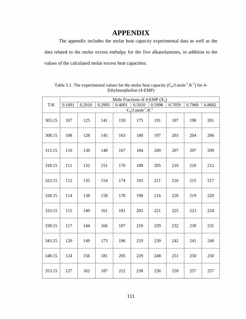
111

APPENDIX The appendix includes the molar heat capacity experimental data as well as the

data related to the molar excess enthalpy for the five alkanolamines, in addition to the

values of the calculated molar excess heat capacities.

Table 5.1. The experimental values for the molar heat capacity (Cp/J.mole-1

.K-1

) for 4-

Ethylmorpholine (4-EMP)

T/K

Mole Fractions of 4-EMP (X1)

0.1001 0.2010 0.2995 0.4001 0.5010 0.5998 0.7059 0.7960 0.8682

Cp/J.mole-1

.K-1

303.15 107 125 141 159 175 191 197 198 201

308.15 108 128 145 163 180 197 203 204 206

313.15 110 130 148 167 184 200 207 207 209

318.15 111 132 151 170 188 205 210 210 212

323.15 112 135 154 174 193 211 216 215 217

328.15 114 138 158 178 198 216 220 219 220

333.15 115 140 161 181 203 221 225 223 224

338.15 117 144 166 187 210 229 232 230 231

343.15 120 149 173 196 219 239 242 241 240

348.15 124 156 181 205 229 248 251 250 250

353.15 127 162 187 212 238 256 259 257 257

112

Table 5.2. The experimental values for the molar heat capacity (Cp/J.mole-1

.K-1

) for

1-Dimethylamino-2-propanol (1-DEAP)

T/K

Mole Fractions of 1-DEAP(X1)

0.1001 0.2010 0.2995 0.4001 0.5010 0.5998 0.7059 0.7960 0.8682

Cp/J.mole-1

.K-1

303.15 111 135 157 170 183 198 216 232 245

308.15 114 139 161 175 188 202 220 236 249

313.15 116 143 166 180 194 208 225 241 253

318.15 118 147 171 184 199 213 230 246 258

323.15 120 150 176 190 205 219 236 251 263

328.15 123 155 182 197 212 225 242 257 269

333.15 126 159 188 203 218 232 248 263 275

338.15 129 164 193 209 225 239 255 270 281

343.15 132 170 202 218 233 247 263 277 288

348.15 137 178 212 229 245 258 273 286 296

353.15 143 187 224 244 259 271 286 297 306

113

Table 5.3. The experimental values for the molar heat capacity (Cp/J.mole-1

.K-1

) for

2-(Diisopropylamino)ethanol (2-DPAE)

T/K

Mole Fractions of 2-DPAE (X1)

0.1001 0.2010 0.2995 0.4001 0.5010 0.5998 0.7059 0.7960 0.8682

Cp/J.mole-1

.K-1

303.15 123 159 191 224 258 287 308 321 332

308.15 125 161 194 228 262 291 312 325 335

313.15 126 163 196 230 265 294 314 327 338

318.15 127 165 198 233 268 297 317 329 339

323.15 128 167 201 236 271 300 320 332 341

328.15 129 169 204 239 275 304 323 335 344

333.15 131 172 208 243 279 308 326 338 347

338.15 132 174 211 247 283 312 330 341 350

343.15 134 177 214 251 288 318 335 345 352

348.15 137 180 217 254 292 322 339 348 354

353.15 139 183 221 259 296 325 341 350 355

114

Table 5.4. The experimental values for the molar heat capacity (Cp/J.mole-1

.K-1

) for

3-Dimethylamino-1-propanol (3-DEAP)

T/K

Mole Fractions of 3-DEAP (X1)

0.1001 0.2010 0.2995 0.4001 0.5010 0.5998 0.7059 0.7960 0.8682

Cp/J.mole-1

.K-1

303.15 105 126 142 159 178 198 205 213 221

308.15 105 127 144 161 180 200 207 215 223

313.15 107 129 147 165 184 203 211 219 227

318.15 108 132 150 168 188 207 215 223 231

323.15 110 135 154 172 192 212 221 228 235

328.15 112 138 158 177 197 217 226 233 240

333.15 114 142 162 182 203 223 232 238 244

338.15 117 146 167 188 210 231 240 245 250

343.15 119 151 173 195 216 238 246 251 256

348.15 122 155 179 201 223 245 254 258 262

353.15 125 159 184 208 231 252 262 265 267

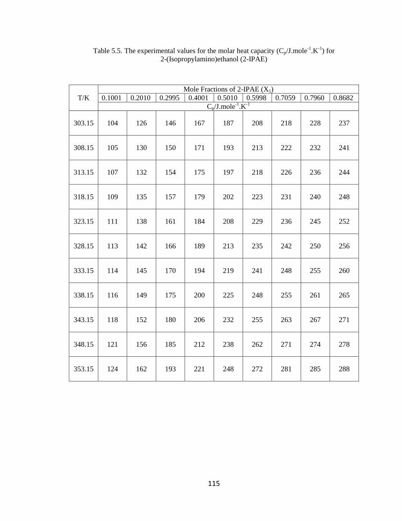
115

Table 5.5. The experimental values for the molar heat capacity (Cp/J.mole-1

.K-1

) for

2-(Isopropylamino)ethanol (2-IPAE)

T/K

Mole Fractions of 2-IPAE (X1)

0.1001 0.2010 0.2995 0.4001 0.5010 0.5998 0.7059 0.7960 0.8682

Cp/J.mole-1

.K-1

303.15 104 126 146 167 187 208 218 228 237

308.15 105 130 150 171 193 213 222 232 241

313.15 107 132 154 175 197 218 226 236 244

318.15 109 135 157 179 202 223 231 240 248

323.15 111 138 161 184 208 229 236 245 252

328.15 113 142 166 189 213 235 242 250 256

333.15 114 145 170 194 219 241 248 255 260

338.15 116 149 175 200 225 248 255 261 265

343.15 118 152 180 206 232 255 263 267 271

348.15 121 156 185 212 238 262 271 274 278

353.15 124 162 193 221 248 272 281 285 288

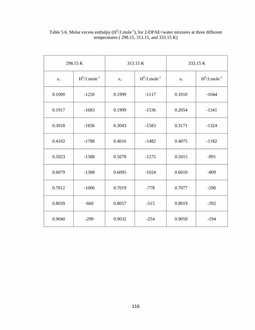
116

Table 5.6. Molar excess enthalpy (HE/J.mole

-1), for 2-DPAE+water mixtures at three different

temperatures ( 298.15, 313.15, and 333.15 K)

298.15 K 313.15 K 333.15 K

x1 HE/J.mole

-1 x1 H

E/J.mole

-1 x1 H

E/J.mole

-1

0.1000 -1250 0.1999 -1117 0.1010 -1044

0.1917 -1683 0.1999 -1536 0.2054 -1341

0.3018 -1836 0.3043 -1583 0.3171 -1324

0.4102 -1788 0.4016 -1482 0.4075 -1182

0.5023 -1588 0.5078 -1275 0.5015 -991

0.6079 -1308 0.6095 -1024 0.6010 -809

0.7012 -1006 0.7019 -778 0.7077 -590

0.8039 -660 0.8057 -515 0.8019 -392

0.9040 -299 0.9032 -254 0.9059 -194

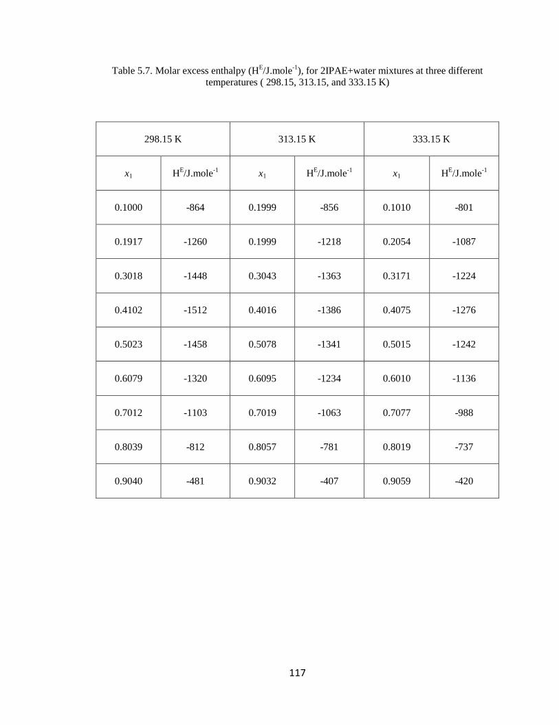
117

Table 5.7. Molar excess enthalpy (HE/J.mole

-1), for 2IPAE+water mixtures at three different

temperatures ( 298.15, 313.15, and 333.15 K)

298.15 K 313.15 K 333.15 K

x1 HE/J.mole

-1 x1 H

E/J.mole

-1 x1 H

E/J.mole

-1

0.1000 -864 0.1999 -856 0.1010 -801

0.1917 -1260 0.1999 -1218 0.2054 -1087

0.3018 -1448 0.3043 -1363 0.3171 -1224

0.4102 -1512 0.4016 -1386 0.4075 -1276

0.5023 -1458 0.5078 -1341 0.5015 -1242

0.6079 -1320 0.6095 -1234 0.6010 -1136

0.7012 -1103 0.7019 -1063 0.7077 -988

0.8039 -812 0.8057 -781 0.8019 -737

0.9040 -481 0.9032 -407 0.9059 -420

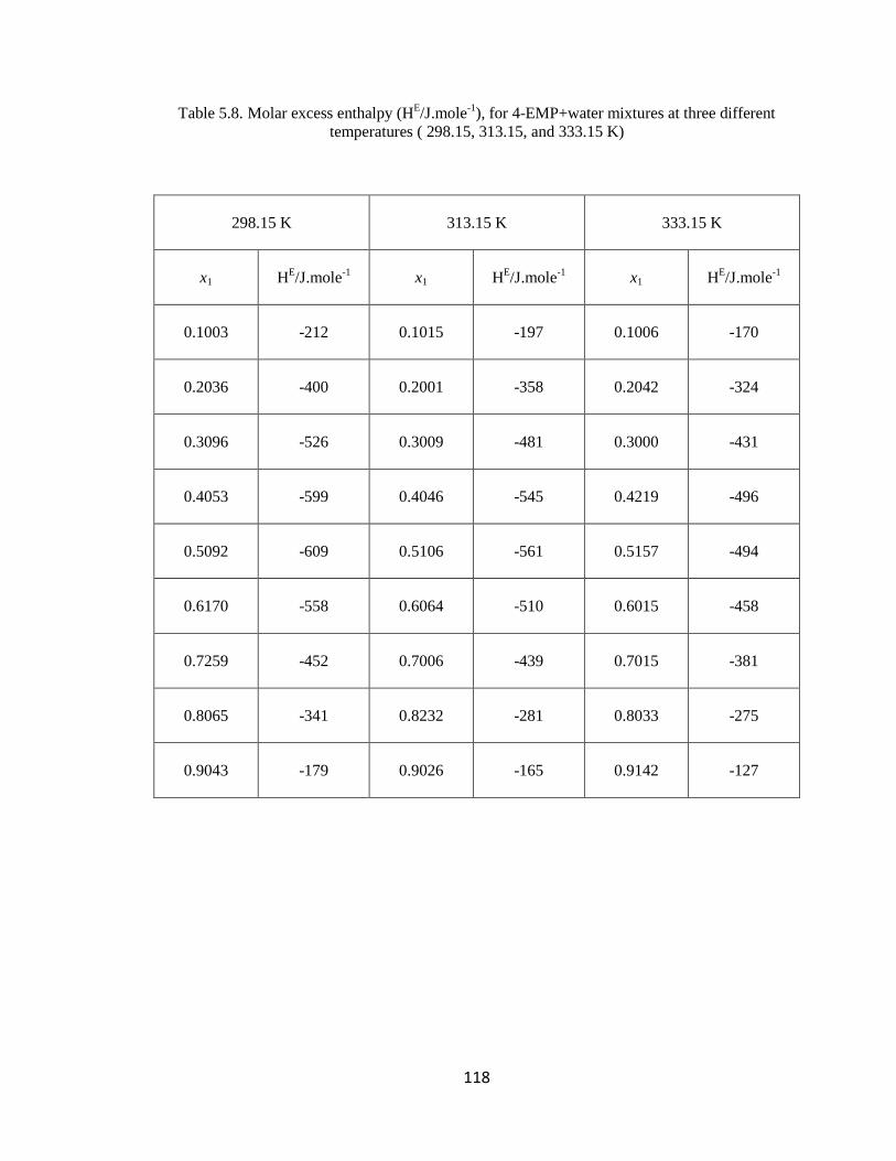
118

Table 5.8. Molar excess enthalpy (HE/J.mole

-1), for 4-EMP+water mixtures at three different

temperatures ( 298.15, 313.15, and 333.15 K)

298.15 K 313.15 K 333.15 K

x1 HE/J.mole

-1 x1 H

E/J.mole

-1 x1 H

E/J.mole

-1

0.1003 -212 0.1015 -197 0.1006 -170

0.2036 -400 0.2001 -358 0.2042 -324

0.3096 -526 0.3009 -481 0.3000 -431

0.4053 -599 0.4046 -545 0.4219 -496

0.5092 -609 0.5106 -561 0.5157 -494

0.6170 -558 0.6064 -510 0.6015 -458

0.7259 -452 0.7006 -439 0.7015 -381

0.8065 -341 0.8232 -281 0.8033 -275

0.9043 -179 0.9026 -165 0.9142 -127

119

Table 5.9. Molar excess enthalpy (HE/J.mole

-1), for 3DEAP+water mixtures at three different

temperatures ( 298.15, 313.15, and 333.15 K)

298.15 K 313.15 K 333.15 K

x1 HE/J.mole

-1 x1 H

E/J.mole

-1 x1 H

E/J.mole

-1

0.1013 -897 0.0735 -651 0.1014 -851

0.2028 -1624 0.1028 -1562 0.1510 -1109

0.3044 -2106 0.2346 -1702 0.2376 -1537

0.4096 -2408 0.3310 -2068 0.3253 -1815

0.5140 -2424 0.4387 -2183 0.4274 -1950

0.6166 -2221 0.5188 -2189 0.6088 -1823

0.7302 -1820 0.7137 -1750 0.7045 -1509

0.8278 -1298 0.7480 -1537 0.8061 -1052

0.9088 -763 0.9085 -623 0.9062 -518

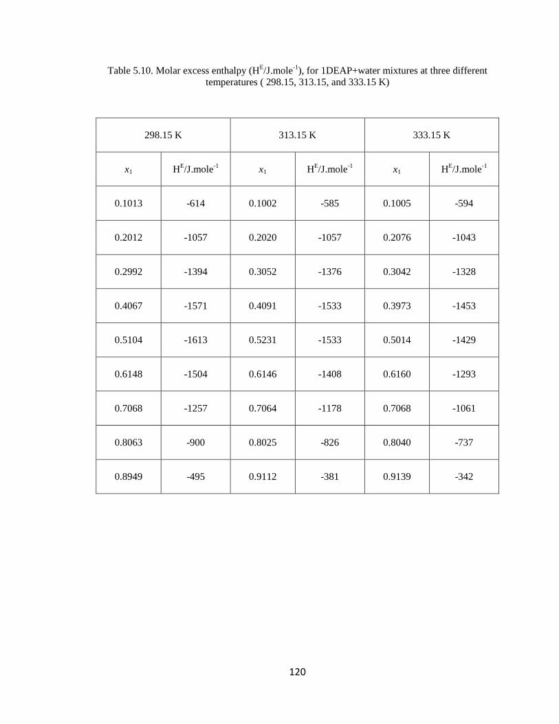
120

Table 5.10. Molar excess enthalpy (HE/J.mole

-1), for 1DEAP+water mixtures at three different

temperatures ( 298.15, 313.15, and 333.15 K)

298.15 K 313.15 K 333.15 K

x1 HE/J.mole

-1 x1 H

E/J.mole

-1 x1 H

E/J.mole

-1

0.1013 -614 0.1002 -585 0.1005 -594

0.2012 -1057 0.2020 -1057 0.2076 -1043

0.2992 -1394 0.3052 -1376 0.3042 -1328

0.4067 -1571 0.4091 -1533 0.3973 -1453

0.5104 -1613 0.5231 -1533 0.5014 -1429

0.6148 -1504 0.6146 -1408 0.6160 -1293

0.7068 -1257 0.7064 -1178 0.7068 -1061

0.8063 -900 0.8025 -826 0.8040 -737

0.8949 -495 0.9112 -381 0.9139 -342