Measuring Benefits from Reduced Air Pollution in the ...iegindia.org/upload/pdf/wp249.pdf · Kolkata in India Using ... consumer surplus benefits from reducing the air pollution from

Measuring Benefits from Reduced Air Pollution in the Cities of Delhi and Kolkata in India Using Hedonic Property Prices Model

M.N. Murty, S.C. Gulati and Avishek Banerjee

Institute of Economic Growth Delhi University Enclave

Delhi-110007 India

August, 2004

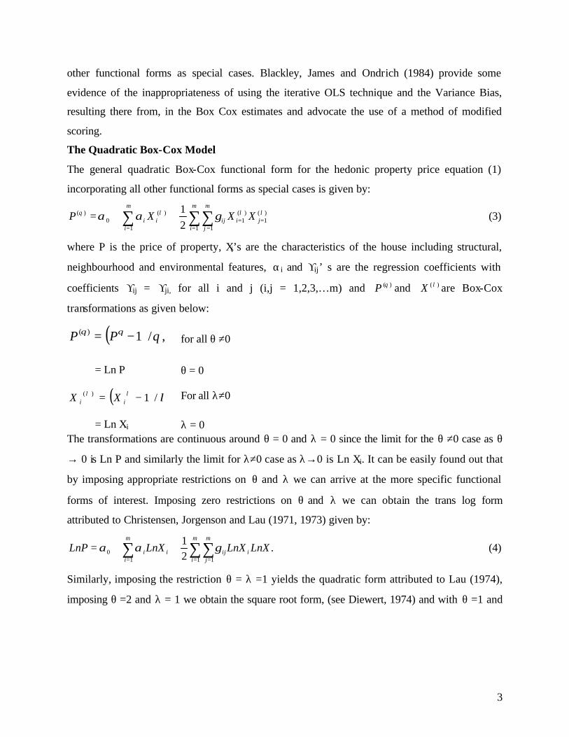
Abstract: This paper* estimates welfare gains to urban households from reduced air pollution in the Indian cities of Delhi and Kolkata using the hedonic property price model. Primary data collected from the household surveys are used in the estimation of model. Alternative estimates of hedonic property price equation and the inverse demand function for atmospheric quality are obtained using the quadratic Box-Cox and trans log specifications. Usually in the empirical literature on hedonic property value models, quadratic Box-Cox specification of property price equation is found to be superior in terms of: (a) various hypotheses tested and (b) in displaying the required curvature property of both the hedonic price equation and inverse demand function for atmospheric quality. Estimates of welfare gains or consumer surplus benefits from reducing the air pollution from the current level to a safe level as defined by WHO or Indian MINAS standards for a representative household and all households in each city are obtained. The estimate of annual benefits from the reduced air pollution to all the households in Delhi and Kolkata are respectively, Rs.54833.1 millions and Rs.37026.2 millions.

JEL Classification: Q 25 Key words: Hedonic property prices, Urban air pollution, Welfare gains, Box-Cox

Contact Address of authors: Institute of Economic Growth, Delhi University Enclave, Delhi-110007, India. Phone: 91-11-27667268 91-11-27667101 Fax: 91-11-27667410 E-mail: [email protected] : [email protected] : [email protected] -------------------------------------------- *This paper forms part of the Research Project, `Valuation and Accounting of Urban Air Pollution: A study of some urban areas in the Indian subcontinent' funded by the South Asian Network of Economic Institutions (SANEI). We are grateful to the participants in the project research workshop at the Institute of Economic Growth, Delhi for useful comments on an earlier draft of this paper.

1

I. Introduction

Commodities could be distinguished by the characteristics they possess and their prices are

functions of these characteristics. From the point of view of the owner, land property could be

distinguished in terms of its location, size, and local environmental quality, while from the

worker’s perspective, a job is a differentiated product in terms of the risk of an on job accident,

working conditions, prestige, training and enhancement of skills, and the local environmental

quality at the work place. Environmental characteristics like air or water quality affect the price

of land either as a producer good or as a consumer good. Ridker (1967) and Ridker and Henning

(1976) provided the first empirical evidence that air pollution affects the property values.

Freeman (1974), and Rosen (1974) used the hedonic price theory to interpret the derivative of

hedonic property price function with respect to air pollution as a marginal implicit price and

therefore the marginal willingness-to-pay of individuals for air pollution reduction. Thaler and

Rosen (1976) are the first to suggest that the labor market could be viewed as the hedonic

market. The derivative of the hedonic wage function with respect to any job characteristic, say

exposure to air pollution at work place, could be interpreted as the marginal implicit price or

worker’s marginal willingness to accept for increased exposure to pollution.

In a hedonic prices model therefore there are two equations to be estimated: The hedonic price

function and the individual’s marginal willingness-to-pay function for the improved environmental

quality1. In the model of hedonic property prices estimated in this paper, the equations are given as:

Phi = Ph (Si, Ni, Qi). (1)

bij = bij ( qj, Qi*,Si, Ni, Gi). (2)

Equation (1) is the hedonic price equation where Phi is the property price2 of the ith house, Si

consists of the structural characteristics of the house, Ni contains the neighborhood

characteristics of the house and Qi stands for the Environmental characteristics of the house.

Equation (2) is the individual’s marginal willingness to `pay function where bij is the marginal

willingness-to-pay for improved air quality for the jth household, while Qi*

is the vector of other

environmental characteristics and Gi stands for socio-economic characteristics. qj is the particular

environmental characteristic for which we want to derive the marginal willingness-to-pay function.

1 See Freeman (1974a) for the derivation of these equations using models explaining consumer choices of private goods, house property, jobs and environmental quality. 2 Here the monthly rental value of the house is taken as a proxy for the property price.

2

There are a number of empirical studies3, mainly in the developed country context, estimating the

hedonic property value model for environmental values. The objective of these studies is to estimate

the hedonic price and the individual’s marginal willingness-to-pay functions with the required

curvature properties. For example, one expects that property prices are an increasing function of the

environmental quality given the characteristics of the house. Similarly, the individual’s marginal

willingness-to-pay is a decreasing function of environmental quality (inverse demand function for

environmental quality) 4.

Obtaining estimates of these functions with the required properties depends upon: (a) Correctness of

data used, and (b) Choice of appropriate functional forms. This paper, using the data collected

through carefully designed household surveys in Delhi and Kolkata, the two important urban areas

in India, explains the importance of choice of appropriate functional forms in the estimation of the

hedonic property value model and provides estimates of consumer surplus benefits to households in

both the cities from reducing air pollution to the safe level.

II. Choice of Functional Forms in Hedonic Price Models

The choice of functional form has usually been restricted both by theoretically unwarranted

restrictions and by convenience in dealing with the problem at hand. As a result in most of the

studies, a linear or a semi- log and at most a trans log model has been widely used. Griliches

(1967) suggested the use of the Box Cox (1964) methodology for choosing among alternative

functional forms under a relevant statistical framework. The early exception from the over

restrictive theoretical framework was noted in Goodman (1978). The flexible functional form

includes the quadratic, translog, square root quadratic, generalized square root and generalized

Leontief. However, Halvorsen and Pollakowski (1981) provide a lucid discus sion on the

combination of the Box Cox and the flexible functional form approaches. They specify a

generalized functional form, namely the quadratic Box Cox functional form, which yields all

3 Ridker (1967) and Rid ker and Henning (1976) provide the first empirical evidence that air pollution affects the property values.

The early studies include Freeman (1974a; 1974b), Anderson and Crocker (1971; 1972), Lind (1973), Pines and Weiss (1976),

Polinsky and Shavell (1976), Nelson (1978), Portney (1981), Horowitz (1986), Murdoch and Thayer (1988), and Kanemoto

(1988). The most recent studies include the following: Michaels and Smith (1990), Parsons (1992), Lansford and Jones (1995),

Kiel (1995), Kiel and McClain (1995), and Mahan, Polasky, and Adams (2000). Rrecent studies in India: are Parikh (1994), Sen

(1994) and Murty, Gulati and Banerjee (2003). 4 Some studies have failed to obtain inverse an demand function for environmental quality for example, Mahan, Polasky, and Adams (2000).

3

other functional forms as special cases. Blackley, James and Ondrich (1984) provide some

evidence of the inappropriateness of using the iterative OLS technique and the Variance Bias,

resulting there from, in the Box Cox estimates and advocate the use of a method of modified

scoring.

The Quadratic Box-Cox Model

The general quadratic Box-Cox functional form for the hedonic property price equation (1)

incorporating all other functional forms as special cases is given by:

∑ ∑∑= = =

==++=m

i

m

i

m

jjiijii XXXP

1 1 1

)(1

)(1

)(0

)(

21 λλλθ γαα (3)

where P is the price of property, Xi’s are the characteristics of the house including structural,

neighbourhood and environmental features, αi and ϒij’ s are the regression coefficients with

coefficients ϒij = ϒji, for all i and j (i,j = 1,2,3,…m) and )(θP and )(λX are Box-Cox

transformations as given below:

( ) ,/1)( θθθ −= PP for all θ ≠0

= Ln P θ = 0

( ) λλλ /1)( −= ii XX For all λ≠0

= Ln Xi λ = 0 The transformations are continuous around θ = 0 and λ = 0 since the limit for the θ ≠0 case as θ

→ 0 is Ln P and similarly the limit for λ≠0 case as λ→0 is Ln Xi. It can be easily found out that

by imposing appropriate restrictions on θ and λ we can arrive at the more specific functional

forms of interest. Imposing zero restrictions on θ and λ we can obtain the trans log form

attributed to Christensen, Jorgenson and Lau (1971, 1973) given by:

∑∑∑= ==

++=m

i

m

jiij

m

iii LnXLnXLnXLnP

1 110 .

21

γαα (4)

Similarly, imposing the restriction θ = λ =1 yields the quadratic form attributed to Lau (1974),

imposing θ =2 and λ = 1 we obtain the square root form, (see Diewert, 1974) and with θ =1 and

4

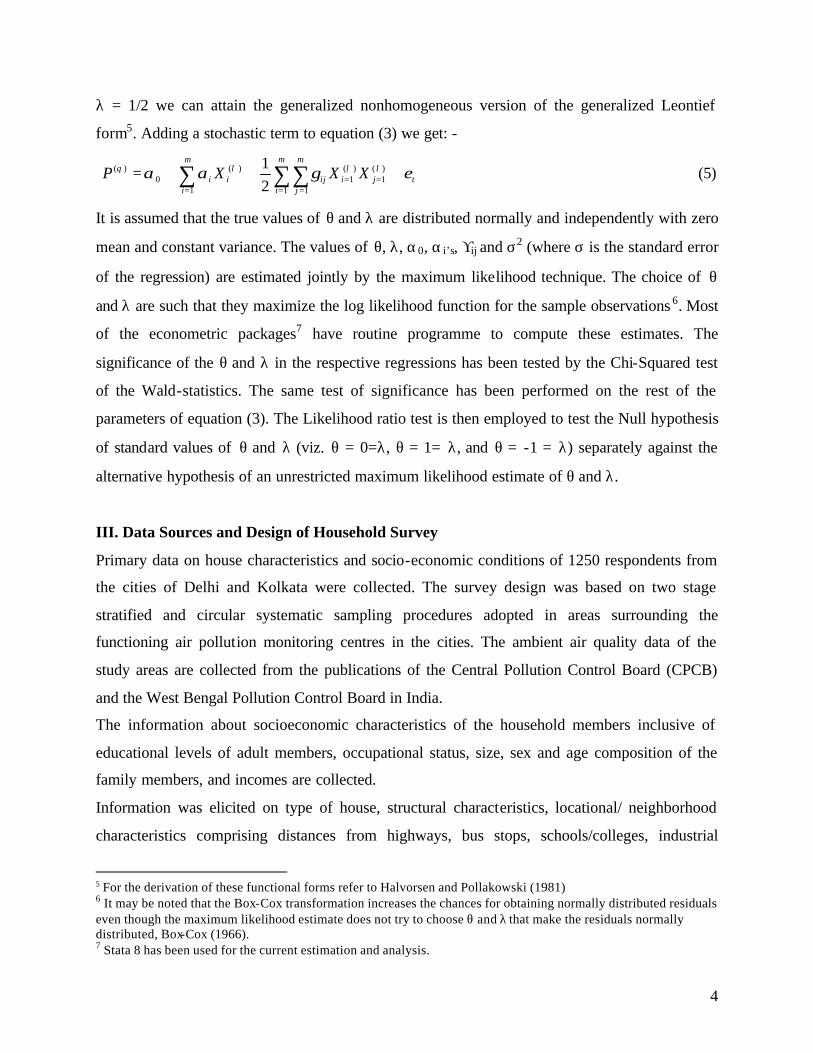
λ = 1/2 we can attain the generalized nonhomogeneous version of the generalized Leontief

form5. Adding a stochastic term to equation (3) we get: -

t

m

i

m

i

m

jjiijii XXXP εγαα λλλθ +++= ∑ ∑∑

= = ===

1 1 1

)(1

)(1

)(0

)(

21

(5)

It is assumed that the true values of θ and λ are distributed normally and independently with zero

mean and constant variance. The values of θ, λ, α0, αi’s, ϒij and σ2 (where σ is the standard error

of the regression) are estimated jointly by the maximum likelihood technique. The choice of θ

and λ are such that they maximize the log likelihood function for the sample observations 6. Most

of the econometric packages7 have routine programme to compute these estimates. The

significance of the θ and λ in the respective regressions has been tested by the Chi-Squared test

of the Wald-statistics. The same test of significance has been performed on the rest of the

parameters of equation (3). The Likelihood ratio test is then employed to test the Null hypothesis

of standard values of θ and λ (viz. θ = 0=λ, θ = 1= λ, and θ = -1 = λ) separately against the

alternative hypothesis of an unrestricted maximum likelihood estimate of θ and λ.

III. Data Sources and Design of Household Survey

Primary data on house characteristics and socio-economic conditions of 1250 respondents from

the cities of Delhi and Kolkata were collected. The survey design was based on two stage

stratified and circular systematic sampling procedures adopted in areas surrounding the

functioning air pollution monitoring centres in the cities. The ambient air quality data of the

study areas are collected from the publications of the Central Pollution Control Board (CPCB)

and the West Bengal Pollution Control Board in India.

The information about socioeconomic characteristics of the household members inclusive of

educational levels of adult members, occupational status, size, sex and age composition of the

family members, and incomes are collected.

Information was elicited on type of house, structural characteristics, locational/ neighborhood

characteristics comprising distances from highways, bus stops, schools/colleges, industrial

5 For the derivation of these functional forms refer to Halvorsen and Pollakowski (1981) 6 It may be noted that the Box-Cox transformation increases the chances for obtaining normally distributed residuals even though the maximum likelihood estimate does not try to choose θ and λ that make the residuals normally distributed, Box-Cox (1966). 7 Stata 8 has been used for the current estimation and analysis.

5

complexes, public parks, etc. was also elicited. Further, information on community

characteristics like majority religion, dominant professional group, and crime rate in the locality

was collected. Information on the respondent’s perception of the environmental

conditions/characteristics such as the air quality, water quality, extent of green cover, etc. was

also collected.

Detailed information on prices of properties was also elicited from the respondents. To cross

check, the property prices obtained from the respondents in the survey, data on property prices

were also collected from the property dealers in the surveyed areas. We surveyed 1250

households from each city expecting that information could be obtained completely for at least

1000 households per city. The sample size was divided equally around the functioning air

pollution monitoring stations in the two cities. For illustration, the sample size of 1250 in Delhi

was divided into a sub-sample size of around 180 around each of the 7 pollution-monitoring

stations of the Central Pollution Control Board (CPCB). In Kolkata the sample size of around 65

was fixed around 19 air-pollution monitoring centres monitored by the West Bengal Pollution

Control Boards (WBPCB). Ultimately, full information could be obtained only for 1187

households in Delhi and 1204 households in Kolkata. Thus, the first stage of stratification was

geographic which was purposive in the sense that the localities around the monitoring stations

were the selection criterion for the locality.

In the second stage, in each city the inhabited localities around the monitoring stations were

stratified according to the type of locality adjudged by the standards of living of the inhabitants

in terms of size of the houses, types of the houses such as bungalows/ independent houses or

flats, type of conveyances used in general, etc. through physical verification by visiting the areas.

At this stage, three localities one each from the high, medium and low income category were

identified to draw a sample comprising a whole range of households in terms of socioeconomic

status. The identification and mapping of localities selected for the survey has provided the

necessary framework for selecting the households in the third stage. The selection of the targeted

number of households was done by adopting a circular systematic sampling procedure in each

selected locality nearer to the monitoring station.

6

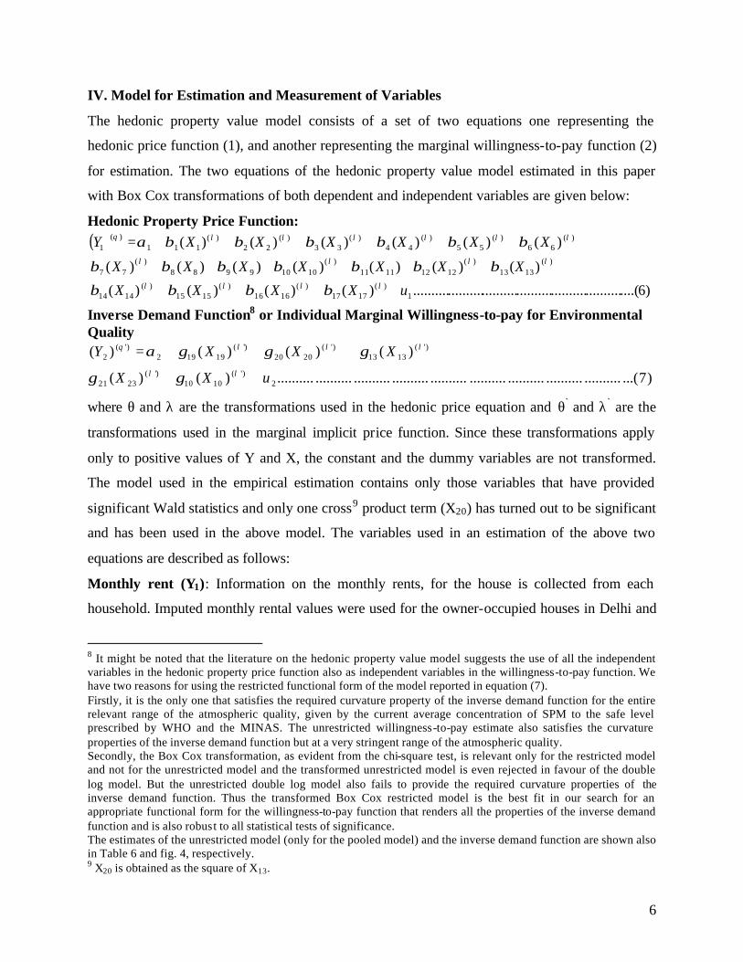
IV. Model for Estimation and Measurement of Variables

The hedonic property value model consists of a set of two equations one representing the

hedonic price function (1), and another representing the marginal willingness-to-pay function (2)

for estimation. The two equations of the hedonic property value model estimated in this paper

with Box Cox transformations of both dependent and independent variables are given below:

Hedonic Property Price Function: ( )

)6....(............................................................)()()()(

)()()()()()()(

)()()()()()(

1)(

1717)(

1616)(

1515)(

1414

)(1313

)(12121111

)(10109988

)(77

)(66

)(55

)(44

)(33

)(22

)(111

)(1

uXXXX

XXXXXXX

XXXXXXY

++++

+++++++

+++++++=

λλλλ

λλλλ

λλλλλλθ

ββββ

βββββββ

ββββββα

Inverse Demand Function8 or Individual Marginal Willingness-to-pay for Environmental Quality

)7...(..........................................................................................)()(

)()()()(

2)'(

1010)'(

2321

)'(1313

)'(2020

)'(19192

)'(2

uXX

XXXY

++

++++=λλ

λλλθ

γγ

γγγα

where θ and λ are the transformations used in the hedonic price equation and θ` and λ` are the

transformations used in the marginal implicit price function. Since these transformations apply

only to positive values of Y and X, the constant and the dummy variables are not transformed.

The model used in the empirical estimation contains only those variables that have provided

significant Wald statistics and only one cross9 product term (X20) has turned out to be significant

and has been used in the above model. The variables used in an estimation of the above two

equations are described as follows:

Monthly rent (Y1): Information on the monthly rents, for the house is collected from each

household. Imputed monthly rental values were used for the owner-occupied houses in Delhi and

8 It might be noted that the literature on the hedonic property value model suggests the use of all the independent variables in the hedonic property price function also as independent variables in the willingness-to-pay function. We have two reasons for using the restricted functional form of the model reported in equation (7). Firstly, it is the only one that satisfies the required curvature property of the inverse demand function for the entire relevant range of the atmospheric quality, given by the current average concentration of SPM to the safe level prescribed by WHO and the MINAS. The unrestricted willingness-to-pay estimate also satisfies the curvature properties of the inverse demand function but at a very stringent range of the atmospheric quality. Secondly, the Box Cox transformation, as evident from the chi-square test, is relevant only for the restricted model and not for the unrestricted model and the transformed unrestricted model is even rejected in favour of the double log model. But the unrestricted double log model also fails to provide the required curvature properties of the inverse demand function. Thus the transformed Box Cox restricted model is the best fit in our search for an appropriate functional form for the willingness-to-pay function that renders all the properties of the inverse demand function and is also robust to all statistical tests of significance. The estimates of the unrestricted model (only for the pooled model) and the inverse demand function are shown also in Table 6 and fig. 4, respectively. 9 X20 is obtained as the square of X13.

7

Kolkata. Data for monthly rents collected through the survey is compared with the information

about the market rents and property prices collected from the interviews of property dealers from

different localities in Delhi and Kolkata.

Structural Characteristics of the House

Covered area (X1): Data for total covered area of the houses were collected directly from the

households and the figures were reported in square yards. In the case of independent owner

occupied or rented houses care was taken to exclude any uncovered area. For the flats, of course

no such problems was encountered. In the case of multistoried buildings, the covered area was

scaled for the number of floors.

Number of rooms including drawing rooms (X2): The total number of rooms including

drawing room were considered as a control variable for the monthly rental value of the house.

Indoor sanitation (X3): The index for indoor sanitation was constructed out of the following

information: separate kitchen, separate bathrooms and toilets, and condition of indoor

ventilation. The index ranges from 0 to 6. Whenever a facility was found separately in a house it

scored a value of 1 otherwise 0, in this way it can take up to a maximum value of 3 where

separate kitchen, toilet and bathroom facilities are available. For ventilation, a scale of 1 to 3 was

used with a higher number denoting better ventilation. These values were then added to arrive at

the composite scale of 0 to 6.

Distance Characteristics :

Distance from business centre (X4): The distance from any common business centre in the city

was collected from each household.

Distance from national highways (X5): The distance of the house from the national highways

were collected and then an average distance was computed which proxies for the overall distance

of the house from these national highways.

Distance from slum (X6): Distance from the nearby slums was collected for area around each

monitoring station in the cities separately.

Distance from industry (X7): Distance from nearby industries for each monitoring station in

each city was used to control for the extreme conditions of pollution in certain parts of the cities.

8

Distance from shopping centre (X8): The distance from the nearest local shopping complex

was collected for each monitoring station in the cities.

Environmental Variables:

Perception about air quality (X10): This is an ordered variable in the range of 1 to 3, which is

used to rank the locality in terms of the air quality as perceived by the households, the higher the

rank, the higher the air quality available.

Perception about water quality (X12): This is also an ordered variable in the range of 1 to 3,

which is used to rank the locality in terms of the water quality as perceived by the residents of

that area, the higher being the rank, the higher the water quality.

Dummy for Adequacy of Green Cover (X11): This is a 1, 0 binary dummy variable, which is

used to ascertain the perception of a household in any locality about the adequacy of the green

cover (tree cover) in its location.

SPM (X13): The average concentration of SPM in ì gms/m3 in the last 6 months from the month

of survey for a particular locality is used as the pollution variable.

SO2 (X14): The average concentration of SO2 in ì gms/m3 in the last 6 months for a particular

locality is used as the pollution variable.

NOx (X15): The average concentration of NOx in ì gms/m3 in the last 6 months for a particular

locality is used as the pollution variable.

Water supply (X16): The hours of water supply in the particular locality.

Other variables:

Business or salaried class (X9):A dummy variable assigning 1 to business communities and 0 to

salaried class communities.

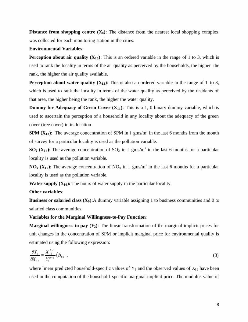
Variables for the Marginal Willingness-to-Pay Function:

Marginal willingness-to-pay (Y2): The linear transformation of the marginal implicit prices for

unit changes in the concentration of SPM or implicit marginal price for environmental quality is

estimated using the following expression:

( )1311

113

13

1 βθ

λ

−

−

=∂∂

Y

X

X

Y, (8)

where linear predicted household-specific values of Y1 and the observed values of X13 have been

used in the computation of the household-specific marginal implicit price. The modulus value of

9

the above expression is used as the dependent variables in the marginal willingness-to-pay

function.

Square of SPM (X20): The square of SPM is used in the second equation keeping in mind the

necessary curvature property of the willingness-to-pay function and its significance of ϒ20 in the

regression. It is expected that the pollution, SPM, positively related to the marginal willingness-

to-pay for reduction in pollution. Alternatively the environmental quality is expected to be

inversely related to the marginal willingness-to-pay. The descriptive statistics of all the selected

variables are presented in the Appendix (Tables A1, A2 and A3).

City Dummy (X23): All the observations belonging to Delhi are marked as 1 and all observations

belonging to Kolkata are marked as 0 in the pooled model.

Socio-economic Variables

Education in years (X18): The education variable is constructed by adding the years of

education undertaken by the first five adult members of the family and dividing by 5.

Annual gross family income (X19): This is based on the gross annual family income of the

household. In the absence of any concrete figures for actual incomes for certain households it

was necessary to offer certain income brackets to the respondents to choose from.

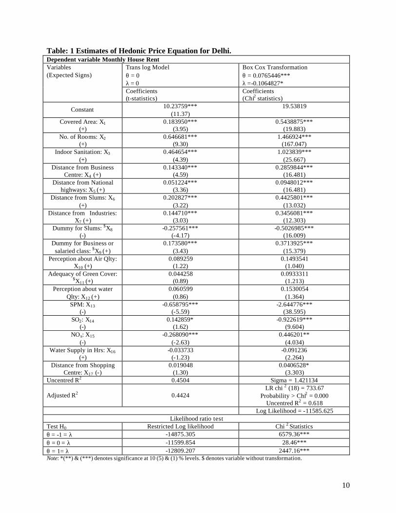
V. Estimates of Hedonic Property Value Model Under Alternative Functional Forms

Estimates of the hedonic property price function for Delhi under the general quadratic Box Cox

estimation and the trans log functional forms are provided in Table 1. In both the estimates the

structural variables like Covered Area (X1), Number of rooms (X2), Indoor sanitation (X3) show

the correct sign and is significant at the 1% level. Among the distance characteristics variables

Distance form Business centre (X4), Distance from industries (X7) and Distance from national

highway (X5) are also significant at 1% and bear the correct sign. Distance from slums (X6) and

the dummy for availability of slum (X8) have proper signs and are significant at the 1% level.

The variables measuring the distance from shopping centre (X17) has a positive coefficient and it

is also significant in the unrestricted model.

It is also noted that the presence of business class (X9) affects house rents significantly in both

the model estimates. The Environmental variables like Perception about air quality (X10),

Adequacy of green cover (X11) and Perception about water quality (X12) have expected signs in

both the models but they are not significant. Even hours of water supply (X16) do not seem to

10

Table: 1 Estimates of Hedonic Price Equation for Delhi. Dependent variable Monthly House Rent

Trans log Model θ = 0 λ = 0

Box Cox Transformation θ = 0.0765446*** λ =-0.1064827*

Variables (Expected Signs)

Coefficients (t-statistics)

Coefficients (Chi2 statistics)

Constant 10.23759*** (11.37)

19.53819

Covered Area: X1 (+)

0.183950*** (3.95)

0.5438875*** (19.883)

No. of Rooms: X2 (+)

0.646681*** (9.30)

1.466924*** (167.047)

Indoor Sanitation: X3 (+)

0.464654*** (4.39)

1.023839*** (25.667)

Distance from Business Centre: X4 (+)

0.143340*** (4.59)

0.2859844*** (16.481)

Distance from National highways: X5 (+)

0.051224*** (3.36)

0.0948012*** (16.481)

Distance from Slums: X6 (+)

0.202827*** (3.22)

0.4425801*** (13.032)

Distance from Industries: X7 (+)

0.144710*** (3.03)

0.3456081*** (12.303)

Dummy for Slums: $X8 (-)

-0.257561*** (-4.17)

-0.5026985*** (16.009)

Dummy for Business or salaried class: $X9 (+)

0.173580*** (3.43)

0.3713925*** (15.379)

Perception about Air Qlty: X10 (+)

0.089259 (1.22)

0.1493541 (1.040)

Adequacy of Green Cover: $X11 (+)

0.044258 (0.89)

0.0933311 (1.213)

Perception about water Qlty: X12 (+)

0.060599 (0.86)

0.1530054 (1.364)

SPM: X13 (-)

-0.658795*** (-5.59)

-2.644776*** (38.595)

SO2: X14 (-)

0.142859* (1.62)

-0.922619*** (9.604)

NOx: X15 (-)

-0.268090*** (-2.63)

0.446201** (4.034)

Water Supply in Hrs: X16 (+)

-0.033733 (-1.23)

-0.091236 (2.264)

Distance from Shopping Centre: X17 (-)

0.019048 (1.30)

0.0406528* (3.303)

Uncentred R2 0.4504 Sigma = 1.421134

Adjusted R2 0.4424 LR chi 2 (18) = 733.67

Probability > Chi2 = 0.000 Uncentred R2 = 0.618

Log Likelihood = -11585.625 Likelihood ratio test

Test H0 Restricted Log likelihood Chi 2 Statistics θ = -1 = λ -14875.305 6579.36*** θ = 0 = λ -11599.854 28.46*** θ = 1= λ -12809.207 2447.16*** Note: *(**) & (***) denotes significance at 10 (5) & (1) % levels. $ denotes variable without transformation.

11

affect house rents significantly. The coefficient of the pollution variable, SPM concentration

(X13) is highly significant and has the expected sign in both the models. Given that pollution

concentrations of SO2 and NOx are quite within the safe limits we believe a further reduction or a

slight increase in their concentration would not affect house rents significantly. The uncentred R2

is computed for both the models and it is much higher in the unrestricted model. Other standard

diagnostic tests were performed on these models and both the models are free from any serious

problem10. The likelihood ratio test is also performed on each of the independent variables and

there was no problem of convergence encountered in the process11.

The Likelihood ratio test is employed to test the Null hypothesis of standard values of θ and λ

(viz. θ = 0=λ, θ = 1= λ and θ = -1 = λ) separately against the alternative hypothesis of

unrestricted maximum likelihood estimates of θ and λ. The tests reject the null hypothesis of θ

and λ to be of any of the above standard form against the alternative of unrestricted θ and λ in all

the models estimated in the paper. Thus the quadratic Box Cox estimation is superior when

compared to the parametric estimates of the trans log model (or any other restricted model)

thereby highlighting the importance of the appropriate choice of the functional form for the

hedonic price equation.

The linear predictions of the house rents Y1, were computed from the model estimates of the

hedonic price equation using the appropriate reverse transformation and these were used to

compute the house specific estimates of the marginal implicit prices as shown by equation (8)

above. The expression for Delhi is given by12:

( ) .|644776.2||| 11

113

13

1 −=∂∂

−

−

θ

λ

YX

XY

(9)

The household marginal willingness-to-pay function for the reduction in SPM is estimated by

regressing the implicit marginal prices on income, education and other socioeconomic variables

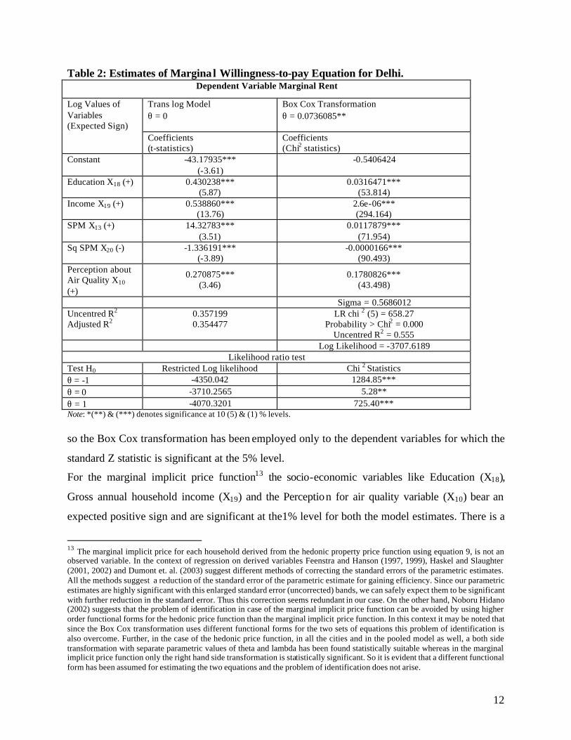
and the SPM concentration and its square. Table 2 provides the parametric estimates of the

marginal willingness-to-pay function under the two models. For this function the standard Z test

does not reject the null hypothesis that lambda is equal to zero even at the10% level of

significance

10 The White’s heteroscedasticity corrected standard errors are reported. 11 For a detailed discussion in the estimation method consult Stata 8 Reference Manual (Vol. 1, A to F). 12 For the trans log model theta and lambda are zero and hence equation (13) reduces to the ratio of X13 to Y1 times the coefficient (-0.658).

12

Table 2: Estimates of Margina l Willingness-to-pay Equation for Delhi. Dependent Variable Marginal Rent

Trans log Model θ = 0

Box Cox Transformation θ = 0.0736085**

Log Values of Variables (Expected Sign)



Constant -43.17935*** (-3.61)

-0.5406424

Education X18 (+) 0.430238*** (5.87)

0.0316471*** (53.814)

Income X19 (+) 0.538860*** (13.76)

2.6e-06*** (294.164)

SPM X13 (+) 14.32783*** (3.51)

0.0117879*** (71.954)

Sq SPM X20 (-) -1.336191*** (-3.89)

-0.0000166*** (90.493)

Perception about Air Quality X10 (+)

0.270875*** (3.46)

0.1780826*** (43.498)

Sigma = 0.5686012 Uncentred R2 Adjusted R2

0.357199 0.354477

LR chi 2 (5) = 658.27 Probability > Chi2 = 0.000

Uncentred R2 = 0.555 Log Likelihood = -3707.6189

Likelihood ratio test Test H0 Restricted Log likelihood Chi 2 Statistics θ = -1 -4350.042 1284.85*** θ = 0 -3710.2565 5.28** θ = 1 -4070.3201 725.40*** Note: *(**) & (***) denotes significance at 10 (5) & (1) % levels.

so the Box Cox transformation has been employed only to the dependent variables for which the

standard Z statistic is significant at the 5% level.

For the marginal implicit price function13 the socio-economic variables like Education (X18),

Gross annual household income (X19) and the Perception for air quality variable (X10) bear an

expected positive sign and are significant at the1% level for both the model estimates. There is a

13 The marginal implicit price for each household derived from the hedonic property price function using equation 9, is not an observed variable. In the context of regression on derived variables Feenstra and Hanson (1997, 1999), Haskel and Slaughter (2001, 2002) and Dumont et. al. (2003) suggest different methods of correcting the standard errors of the parametric estimates. All the methods suggest a reduction of the standard error of the parametric estimate for gaining efficiency. Since our parametric estimates are highly significant with this enlarged standard error (uncorrected) bands, we can safely expect them to be significant with further reduction in the standard error. Thus this correction seems redundant in our case. On the other hand, Noboru Hidano (2002) suggests that the problem of identification in case of the marginal implicit price function can be avoided by using higher order functional forms for the hedonic price function than the marginal implicit price function. In this context it may be noted that since the Box Cox transformation uses different functional forms for the two sets of equations this problem of identification is also overcome. Further, in the case of the hedonic price function, in all the cities and in the pooled model as well, a both side transformation with separate parametric values of theta and lambda has been found statistically suitable whereas in the marginal implicit price function only the right hand side transformation is statistically significant. So it is evident that a different functional form has been assumed for estimating the two equations and the problem of identification does not arise.

13

notable distinction in the signs of X13 and X20 (pollution variables) in the two models. Only

parametric estimates of the unrestricted Box Cox estimation satisfy the required curvature

property of the marginal willingness-to-pay function.

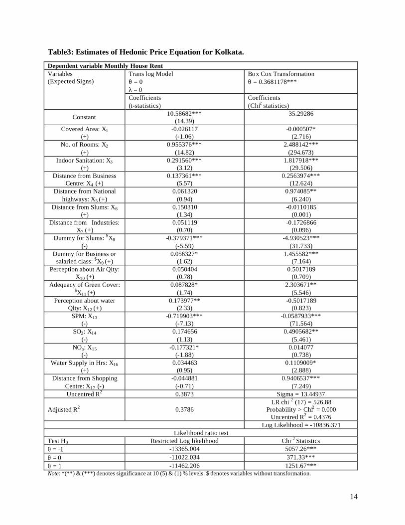
Table 3 provides the parametric estimates of hedonic property price function for Kolkata. In the

case of Kolkata, the Box-Cox transformation is given only to the dependent variable, as the

transformation of the independent variables does not produce any significant change in the

regression as is evident by the Chi2 test. The likelihood ratio test rejects the H0 for all the

standard values of θ tested against the unrestricted value of θ.

In the unrestricted model the regression coefficient for (X13) is quite small when compared to the

same for the Delhi model. However it is highly significant and bears the correct negative sign.

We are again indifferent to the signs picked up by the coefficients of (X14) and (X15) for the

reasons stated above. Among the structural characteristics, the coefficients of (X3) and (X2) have

required positive signs and are highly significant while the coefficient of (X1) bears the opposite

sign and is insignificant in the trans log model while in the unrestricted model it is significant.

The dummy for Slums X8 is significant and negative in both the models while the distance

characteristics produce mixed results for Kolkata as a whole14. Similar to the model for Delhi,

the linear predictions for (Y1) are computed using expression (8) to get the household specific

marginal implicit prices. In this case however exogenous variables are not transformed and so

the expression for the marginal implicit price is:

( ) |0587933.01

||| 1113

1 −=∂∂

−θYXY

(10)

The estimates of marginal willingness-to-pay function for Kolkata are given in Table 4 below.

The coefficients of all the explanatory variables except Income (X19) bear the correct sign and

are highly significant. Even in case of Kolkata the unrestricted model shows the household

diminishing marginal willingness-to-pay for the atmospheric quality.

Two separate estimates of the marginal willingness-to-pay function are made using the pooled

data for Delhi and Kolkata. One estimate is based on the hedonic property price functions

estimated for the segmented house markets Delhi and Kolkata. The implicit marginal prices for

SPM reductions are computed for each market and then pooled. The pooled implicit marginal

14 They are still more effective in case of the unrestricted model (e.g. X5 and X17).

14

Table3: Estimates of Hedonic Price Equation for Kolkata.

Dependent variable Monthly House Rent Trans log Model θ = 0 λ = 0

Box Cox Transformation θ = 0.3681178***

Variables (Expected Signs)



Constant 10.58682*** (14.39)

35.29286

Covered Area: X1 (+)

-0.026117 (-1.06)

-0.000507* (2.716)

No. of Rooms: X2 (+)

0.955376*** (14.82)

2.488142*** (294.673)

Indoor Sanitation: X3 (+)

0.291560*** (3.12)

1.817918*** (29.506)

Distance from Business Centre: X4 (+)

0.137361*** (5.57)

0.2563974*** (12.624)

Distance from National highways: X5 (+)

0.061320 (0.94)

0.974085** (6.240)

Distance from Slums: X6 (+)

0.150310 (1.34)

-0.0110185 (0.001)

Distance from Industries: X7 (+)

0.051119 (0.70)

-0.1726866 (0.096)

Dummy for Slums: $X8 (-)

-0.379371*** (-5.59)

-4.930523*** (31.733)

Dummy for Business or salaried class: $X9 (+)

0.056327* (1.62)

1.455582*** (7.164)

Perception about Air Qlty: X10 (+)

0.050404 (0.78)

0.5017189 (0.709)

Adequacy of Green Cover: $X11 (+)

0.087828* (1.74)

2.303671** (5.546)

Perception about water Qlty: X12 (+)

0.173977** (2.33)

-0.5017189 (0.823)

SPM: X13 (-)

-0.719903*** (-7.13)

-0.0587933*** (71.564)

SO2: X14 (-)

0.174656 (1.13)

0.4905682** (5.461)

NOx: X15 (-)

-0.177321* (-1.88)

0.014077 (0.738)

Water Supply in Hrs: X16 (+)

0.034463 (0.95)

0.1109009* (2.888)

Distance from Shopping Centre: X17 (-)

-0.044881 (-0.71)

0.9406537*** (7.249)

Uncentred R2 0.3873 Sigma = 13.44937

Adjusted R2 0.3786 LR chi 2 (17) = 526.88

Probability > Chi2 = 0.000 Uncentred R2 = 0.4376


Test H0 Restricted Log likelihood Chi 2 Statistics θ = -1 -13365.004 5057.26*** θ = 0 -11022.034 371.33*** θ = 1 -11462.206 1251.67*** Note: *(**) & (***) denotes significance at 10 (5) & (1) % levels. $ denotes variables without transformation.

15

Table 4: Estimates of Marginal Willingness-to-pay Equation for Kolkata Dependent Variable Marginal Rent



Log Values of Variables (Expected Sign) Coefficients

(t-statistics) Coefficients (Chi2 statistics)

Constant -22.96979** (-2.48)

3.069313

Education X18 (+) 0.796318*** (6.94)

0.0119188*** (22.779)

Income X19 (+) 0.571237*** (11.52)

-2.42e-07*** (9.191)

SPM X13 (+) 6.737927** (2.07)

0.0021936*** (10.354)

Sq SPM X20 (-) -0.693091** (-2.42)

-3.63e-06*** (11.905)


0.173072*** (3.30)

0.0336502*** (10.415)


0.333585 0.330727

LR chi 2 (5) = 61.23 Probability > Chi2 = 0.000

Uncentred R2 = 0.50 Log Likelihood = -3707.6189

Likelihood ratio test Test H0 Restricted Log likelihood Chi 2 Statistics θ = -1 -1421.3999 49.53*** θ = 0 -1399.136 5.01** θ = 1 -1399.4891 5.71** Note: *(**) & (***) denotes significance at 10 (5) & (1) % levels.

prices are regressed on the SPM levels and the socioeconomic characteristics of households

along with a city specific dummy variable (X23). This is one approach to deal with the

econometric problem of identification in the estimation of the household marginal willingness-

to-pay function in the hedonic property value model as discussed in Freeman (1993). Another

estimate is based on the hedonic property price function estimated using the pooled data for

Delhi and Kolkata. However, we are reporting the results of only the marginal willingness-to-pay

function for the pooled model estimated by using the market segmentation approach15.

The parametric estimates of the two models have the proper sign and are highly significant. In

this case also, the curvature property is satisfied by the unrestricted model only. The likelihood

ratio test rejects H0 for all standard forms of θ and thus the unrestricted model is unambiguously

superior to the trans log counterparts16 in the estimates for both the cities as well as the pooled

15 The complete set of results of the pooled model is available on request from the authors. 16 All standard transformations are rejected in favour of the unrestricted quadratic Box Cox transformation.

16

model. Further, only by following the segmented market approach in the case of pooled model

estimates, the required curvature property was satisfied.

Table 5: Estimates of Marginal Willingness-to-pay Equation for the pooled model Dependent Variable Marginal Rent



Log Values of Variables (Expected Sign)



Constant -30.62877*** (-5.25)

0.4782014

Education X18 (+) 0.558753*** (9.23)

0.013794*** (88.590)

Income X19 (+) 0.554709*** (18.01)

8.87e -07*** (325.828)

SPM X13 (+) 9.689258*** (4.77)

0.0052934*** (228.374)

Sq SPM X20 (-) -0.950415*** (-5.42)

-7.7e-06*** (258.450)


0.221595*** (5.05)

0.0477618*** (40.216)

City Dummy X23 (+) 0.790453*** (21.48)

0.214818*** (327.223)


0.42295 0.42148

LR chi 2 (6) = 1096.25 Probability > Chi2 = 0.000 Uncentred R2 = 0.46372


Test H0 Restricted Log likelihood Chi 2 Statistics θ = -1 -7116.5125 1485.73*** θ = 0 -6400.8154 54.33** θ = 1 -7502.4537 2257.61** Note: *(**) & (***) denotes significance at 10 (5) & (1) % levels.

Ideally, one could expect that the similar sets of structural and neighbourhood variables (as used

in the estimation of the Hedonic price function) along with the environmental and socioeconomic

characteristics determine the marginal willingness-to-pay for environmental quality. However in

the current study, it has been observed that the parametric estimates of the pollution variables

remain unaffected with the inclusion of the structural and environmental characteristics in the

marginal willingness-to-pay function. The robustness of the parametric estimates can be

attributed to the weak separability between the Environmental variables with the Structural and

Neighbourhood characteristics while determining the marginal willingness-to-pay for clean air.

The parametric estimate of the unrestricted17 marginal willingness-to-pay is provided in Table 6

below. The Likelihood ratio test rejects the double log model as well as all other standard 17 Using all the independent variables that were used in the hedonic price function.

17

functional forms of the marginal willingness-to-pay function in favour of the both sides

transformed unrestricted model. Also in the both sides transformation model the individual z-test

rejects the null hypothesis that the true value of λ and θ are zero. However all single-sided

transformations or double-sided transformation with the same parameter of the unrestricted

model are rejected in favour of the double log model and render insignificant parametric

estimates of λ and θ as well. Thus it is easy to conclude that the both side transformation model

is more appropriate than any other model in terms of statistical analysis. But unfortunately, even

the both side transformation model fails to offer the required curvature property of the inverse

demand function in the relevant range 18, just as any other functional form of the unrestricted

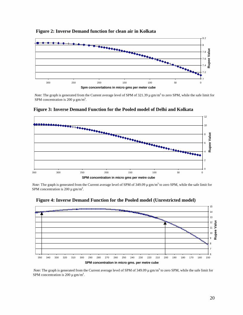
model. Figure 4 represents the inverse demand function estimated form the unrestricted model.

The market segmentation approach has been followed for all the pooled data estimates.

The unrestricted willingness-to-pay function fails to provide the required curvature properties in

the individual city-specific19 models as well. Thus the welfare gains obtained from a reduction of

air pollution have been computed only from the restricted model of the marginal willingness-to-

pay function.

18 The relevant range is defined as the current average concentration of SPM to the WHO, MINAS prescribed safe level of 200 µ gm/m3. 19 These estimates are not reported here.

18

Table 6: Estimates of Marginal Willingness-to-pay Equation for the pooled model (Unrestricted)

Dependent Variable Marginal Rent Box Cox Transformation parameters Theta = -0.0526165 *** Lambda = -0.3364357***

Variables Coefficients (Chi2 statistics)

Variables Coefficients (Chi2 statistics)

Constant -316.5959 Dummy for Business or salaried class: $X9

0.3092857*** (26.029)

Covered Area: X1

0.826*** (431.178)

Perception about Air Qlty: X10 0.0274651*** (13.754)

No. of Rooms: X2

0.0340558*** (332.138)

Adequacy of Green Cover: $X11 0.0043971*** (0.187)

Indoor Sanitation: X3

0.0495319*** (140.092)

Perception about water Qlty: X12 0.0107325** (4.572)

Distance from Business Centre: X4

0.0631395*** (129.693)

SPM: X13

-42.17456*** (408.905)

Distance from National highways: X5

0.0312554*** (331.616)

Sq SPM X20 141.5829*** (404.324)

Distance from Slums: X6 0.2264228*** (198.459)

Water Supply in Hrs: X16 -0.0302438*** (8.623)

Distance from Industries: X7 0.1892529*** (728.652)

Distance from Shopping Centre: X17 0.0093668*** (35.112)

Dummy for Slums: $X8

-0.2085701*** (858.672)

LR chi 2 (20) = 2929.85 Probability > Chi2 = 0.000 Uncentred R2 = 0.78 Log Likelihood = -5268.4761

Likelihood ratio test

Test H0 Restricted Log

likelihood Chi 2 Statistics Test H0

θ = -1 -6449.8946 2362.84*** θ = -1 θ = 0 -5541.989 547.03*** θ = 0 θ = 1 -6674.0822 2811.21*** θ = 1 Note: *(**) & (***) denotes significance at 10 (5) & (1) % levels.

V. Inverse Demand Functions for Environmental Quality and Welfare Gains from Reduced Air Pollution By fixing variables X18, X19 and X10 in the estimated20 equations of marginal willingness-to-pay

at their sample mean values, and treating pollution variables (X13) and (X20) as the only variable,

the inverse demand function21 for clean air was derived. After applying the appropriate reverse

transformation, the linearized22 predicted values of marginal willingness-to-pay (MWP) in the

20 Given in Tables 2, 4 and 6 for Delhi, Kolkata and the Pooled model, respectively. 21 This is also the marginal willingness-to-pay function for clean air. 22 The reverse linear transformation refers to the Y = (1 + θα0 + θΣαiXi)

1/θ in which anything other than X13 and X20 are set at their mean values.

19

inverse demand functions for Delhi, Kolkata and the Pooled model are given by equations (11),

(12) and (13). The reverse transformation is necessary in order to express the predicted values of

marginal willingness-to-pay, out of the Box Cox transformed variables, in the actual rupee

values, given that Monthly rent (Y1) is expressed in rupees.

MWP = [1.051322 + 0.0008677 X13 – 0.0000012 X20]13.585 [Delhi] (11)

MWP = [2.560514 + 0.0010512 X13 – 0.0000017 X20]2.0867 [Kolkata] (12)

MWP = [0.826114 + 0.0009079 X13 – 0.0000013 X20]13.585 [Pooled] (13)

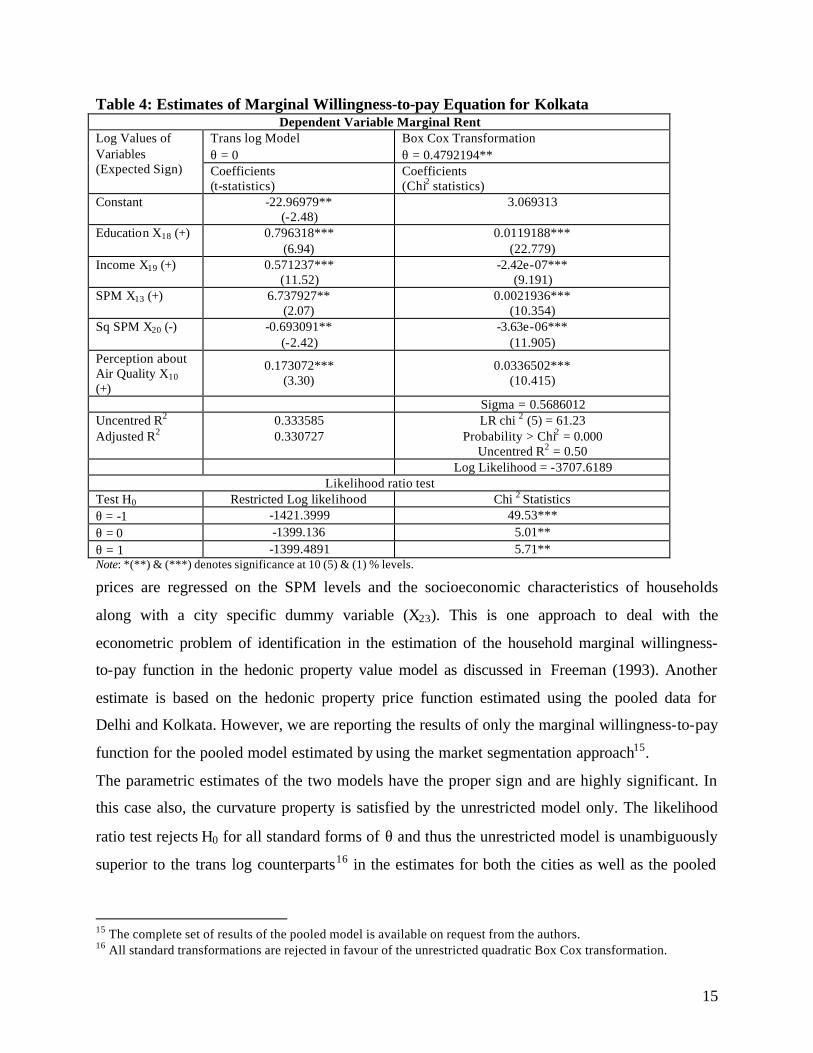
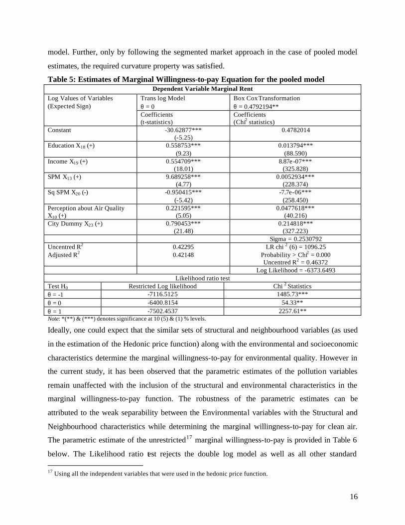
From the above estimates of the inverse demand function the margina l willingness-to-pay, for a

typical household, for a reduction in SPM concentration by one micro gram per metre cube from

the current average level of pollution, is computed as Rs.12.63 for Delhi, Rs.8.06 for Kolkata

and Rs.10.21 for a representative household in the pooled model. By using suitable dummies for

the cities and the city-specific SPM concentrations the willingness-to-pay for reduction in SPM

concentration by one micro gram per meter cube from the current average level of pollution, is

computed as Rs.12.01 in Delhi and Rs.8.74 in Kolkata from the pooled model. The marginal

willingness-to-pay estimated from the individual estimates are thus very close to the estimates

obtained from the pooled model. This shows that the pooled model may be used for extrapolation

of consumer surpluses for any representative city in India using the benefit transfer method. The

graphs of inverse demand functions are shown in figs. 1, 2 and 3, respectively for Delhi, Kolkata

and the pooled model. The SPM concentration is shown in reversed scale on the X-axis to

represent ambient air quality and MWP is shown on the Y-axis

Figure 1: Inverse demand function for clean air in Delhi

0

2

4

6

8

10

12

14

050100150200250300350

SPM concentration in micro gms per metre cube

Rup

ee V

alue

M

Note: The graph is generated from the Current average level of SPM of 366.31 µ gm/m3 to zero SPM, while the safe limit for SPM concentration is 200 µ gm/m3.

20

Figure 2: Inverse Demand function for clean air in Kolkata

7

7.2

7.4

7.6

7.8

8

8.2

050100150200250300

Spm concenrtations in micro gms per meter cube

Rup

ee V

alue


Figure 3: Inverse Demand Function for the Pooled model of Delhi and Kolkata

0

2

4

6

8

10

12

050100150200250300350

SPM concentration in micro gms per metre cube

Rup

ee V

alue


Figure 4: Inverse Demand Function for the Pooled model (Unrestricted model)

6

7

8

9

10

11

12

13

14

15

150160170180190200210220230240250260270280290300310320330340350

SPM concentration in micro gms. per metre cube

Rup

ee V

alue


21

Table 7: Estimates of Welfare Gains to Urban Households in Delhi, Kolkata and for the Pooled Model

Gains to Household Based on Individual

Estimates from Cities

Gains to Household Using Market Segmentation

Approach23 Nature of Gains to Households

Delhi Kolkata Delhi Kolkata Pooled

Monthly gains in Rental value due to reduction of SPM concentration by 1 ì gms/m3

Rs.12.63 Rs.8.06 Rs.12.01 Rs.8.74 Rs.10.21

Monthly gains in Rental value due to reduction of SPM concentration from the current average to the safe level corresponding to 200 ì gms/m3

Rs.1946.14 Rs.977.22 Rs.1887.65 Rs.980.69 Rs.1420.61

Annual gains in Rental value due to reduction of SPM concentration by 1 ì gms/m3

Rs.151.56 Rs.96.72 Rs.144.12 Rs.104.88 Rs.122.52

Annual gains in Rental value due to reduction of SPM concentration from the current average to the safe level corresponding to 200 ì gms/m3

Rs.23353.68 Rs.11726.59 Rs.22651.80 Rs.11768.28 Rs.17047.32

Annual gains in Rental value due to reduction of SPM concentration from the current average to the safe level corresponding to 200 ì gms/m3 to the total Urban Households24.

Rs.54833.08

Million

Rs.37026.16

Million

Rs.53185.10

Million

Rs.37157.78

Million

Rs.92612.69

Million25

23 The estimates of individual cities are calculated by using the city-specific dummy and the city’s average level of pollution. 24 The total urban population is obtained from Census 2001 data and deflated by the average size of household in the respective cities which is 5.46 for Delhi and 4.56.for Kolkata. 25 The total urban population of Delhi and Kolkata is used to evaluate the total gains

23

The consumer surplus generated by a reduction of SPM concentration from the current average

to the safe level of 200 µ gm/m3 is computed by integrating the inverse demand function given

by equations (11) to (13) within 200 µ gm/m3 as the lower limit 26 and the current average level

of pollution in the respective cities as the upper limit. Integration of the inverse demand

functions were carried out in Mathematica27 4.1 and the results of the consumer surpluses are

provided in Table 7 above. The estimated consumer surplus also measures the average

willingness-to-pay by a representative household for reduction in the ambient air pollution from

the current average to the safe WHO or MINAS28 standards. The annual welfare gains to a

typical household from reducing SPM concentration from the current level to the MINAS

standard of 200 ì gms/m3 in Delhi, and Kolkata are respectively, Rs.23353.68 and Rs.11726.59.

According to 2000 census, Delhi and Kolkata have urban populations of 12.8 millions, and 14.4

millions with sample average household sizes of 5.46 and 4.56, respectively. Thus there are

23,47,942, and 31,57,452 estimated urban households in Delhi and Kolkata. The annual benefits

from reduc ing the SPM concentration to safe level in Delhi and Kolkata are respectively

estimated as Rs.54,833.08 million and Rs.37,026.16 million. The estimates of welfare gains to

the two cities as computed form the Pooled model are also given in Table 7. These estimates are

very close to the individual estimates of gains in these cities. This shows the robustness of the

pooled model that may be used in extrapolating welfare gains from a reduction in air pollution in

some other metropolitan centres in India. The welfare gains are not computed from the trans log

model, as the required curvature properties are not satisfied by the inverse demand function.

VI. Conclusion

Empirical studies using the observed behavioral methods (household production function and

hedonic prices models) look for the derivation of an inverse demand function or marginal

willingness-to-pay function for the environmental quality with appropriate curvature properties for

an estimation of the consumer surplus benefits from the improved environmental quality. The

failure to obtain an inverse demand function in some empirical studies might arise either due to: (a)

the poor quality of data used and (b) inappropriate functional form used for the estimation of

hedonic price and willingness-to-pay functions. We have shown that given the reliable data, the 26 200 µ gm/m3 is the safe WHO and MINAS standard for residential area in India. 27 Software for Mathematical Solutions. 28 MINAS: Minimum National Standards for Environmental Pollution in India.

24

inverse demand function with the required properties could be derived with the choice of

appropriate functional form for the hedonic property price and the marginal willingness-to-pay

equations. Starting from a more general quadratic Box Cox functional form for the hedonic price

function a number of functional forms could be considered and tested for their appropriateness.

The hedonic property price function is estimated using the primary data collected for house

characteristics through carefully designed household surveys in Delhi and Kolkata. Estimates of

consumer surplus benefits to a representative household from each city are obtained by integrating

the inverse demand function for air quality in the range of current average quality and the quality

corresponding to safe level.

A representative household gets an annual benefit of Rs.23,353.68 in Delhi and Rs.11,726.59 in

Kolkata. When the benefits are extrapolated to all the urban households in each city, the households

in Delhi get benefits worth Rs.54,833.08 million while those in Kolkata get benefits worth

Rs.37,026.16 million. Though these benefits appear to be high, they are not so in comparison to the

cost to various economic agents like the Government and polluters to reduce the air pollution levels

from the current level to the safe level. In fact these benefit estimates justify the cost of

environmental policy changes like introducing CNG operated vehicles, and substituting the metro

rail in place of road transport and the relocation of polluting industries in the cities.

25

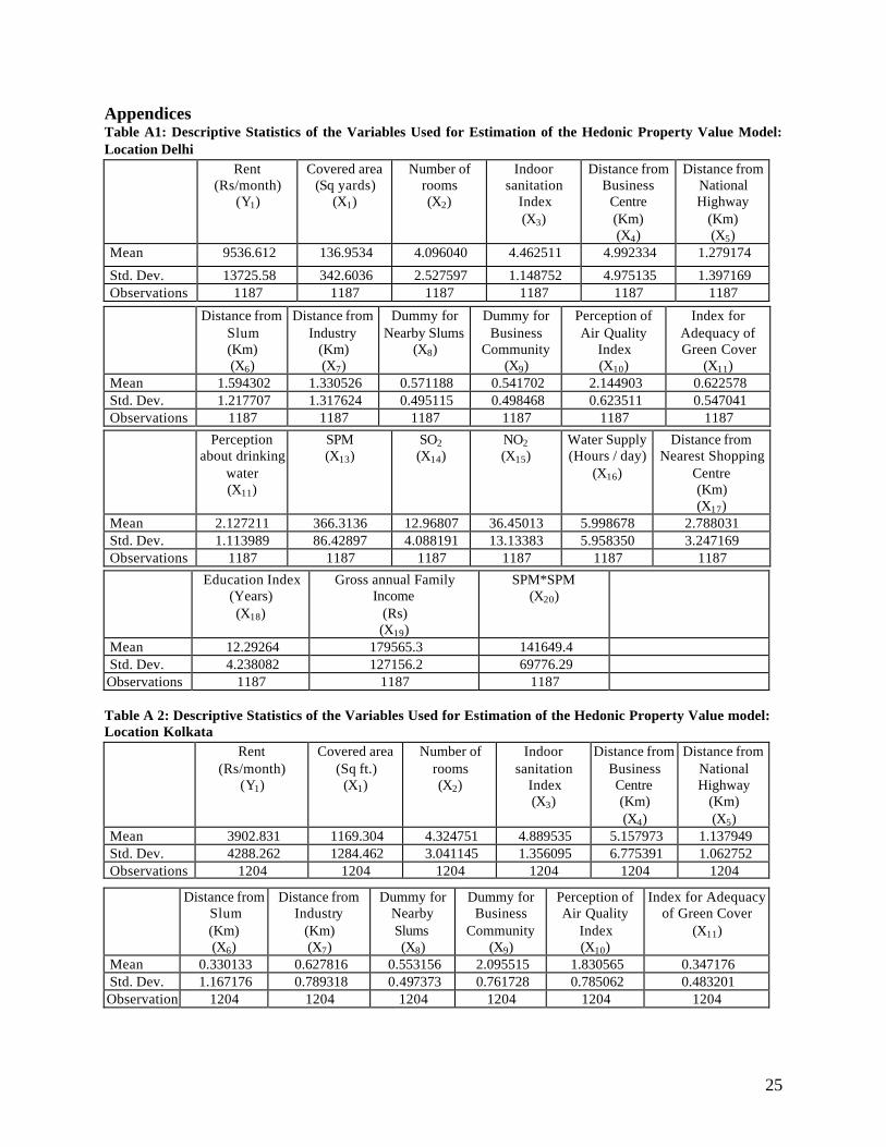
Appendices Table A1: Descriptive Statistics of the Variables Used for Estimation of the Hedonic Property Value Model: Location Delhi

Rent (Rs/month)

(Y1)

Covered area (Sq yards)

(X1)

Number of rooms (X2)

Indoor sanitation

Index (X3)

Distance from Business

Centre (Km) (X4)

Distance from National Highway

(Km) (X5)

Mean 9536.612 136.9534 4.096040 4.462511 4.992334 1.279174

Std. Dev. 13725.58 342.6036 2.527597 1.148752 4.975135 1.397169 Observations 1187 1187 1187 1187 1187 1187

Distance from Slum (Km) (X6)

Distance from Industry

(Km) (X7)

Dummy for Nearby Slums

(X8)

Dummy for Business

Community (X9)

Perception of Air Quality

Index (X10)

Index for Adequacy of Green Cover

(X11) Mean 1.594302 1.330526 0.571188 0.541702 2.144903 0.622578 Std. Dev. 1.217707 1.317624 0.495115 0.498468 0.623511 0.547041 Observations 1187 1187 1187 1187 1187 1187

Perception about drinking

water (X11)

SPM (X13)

SO2 (X14)

NO2 (X15)

Water Supply (Hours / day)

(X16)

Distance from Nearest Shopping

Centre (Km) (X17)

Mean 2.127211 366.3136 12.96807 36.45013 5.998678 2.788031 Std. Dev. 1.113989 86.42897 4.088191 13.13383 5.958350 3.247169 Observations 1187 1187 1187 1187 1187 1187

Education Index (Years) (X18)

Gross annual Family Income

(Rs) (X19)

SPM*SPM (X20)

Mean 12.29264 179565.3 141649.4 Std. Dev. 4.238082 127156.2 69776.29 Observations 1187 1187 1187 Table A 2: Descriptive Statistics of the Variables Used for Estimation of the Hedonic Property Value model: Location Kolkata

Rent (Rs/month)

(Y1)

Covered area (Sq ft.)

(X1)


Indoor sanitation

Index (X3)

Distance from Business Centre (Km) (X4)


(Km) (X5)




(Km) (X7)

Dummy for Nearby Slums (X8)

Dummy for Business

Community (X9)


Index (X10)


(X11)

Mean 0.330133 0.627816 0.553156 2.095515 1.830565 0.347176 Std. Dev. 1.167176 0.789318 0.497373 0.761728 0.785062 0.483201 Observation 1204 1204 1204 1204 1204 1204

26

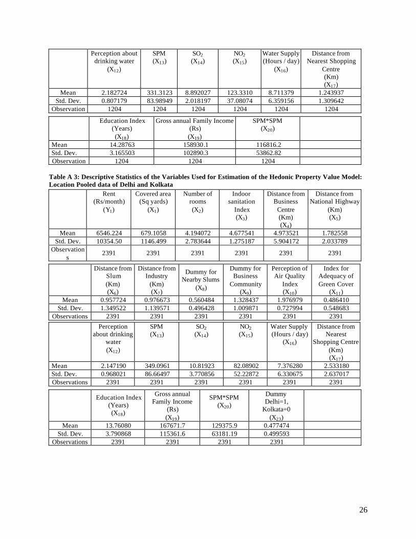
Perception about drinking water

(X12)

SPM (X13)

SO2 (X14)

NO2 (X15)


(X16)

Distance from Nearest Shopping

Centre (Km) (X17)

Mean 2.182724 331.3123 8.892027 123.3310 8.711379 1.243937 Std. Dev. 0.807179 83.98949 2.018197 37.08074 6.359156 1.309642

Observation 1204 1204 1204 1204 1204 1204

Education Index (Years) (X18)

Gross annual Family Income (Rs) (X19)

SPM*SPM (X20)

Mean 14.28763 158930.1 116816.2 Std. Dev. 3.165503 102890.3 53862.82 Observation 1204 1204 1204

Table A 3: Descriptive Statistics of the Variables Used for Estimation of the Hedonic Property Value Model: Location Pooled data of Delhi and Kolkata

Rent (Rs/month)

(Y1)

Covered area (Sq yards)

(X1)


Indoor sanitation

Index (X3)

Distance from Business

Centre (Km) (X4)


(Km) (X5)

Mean 6546.224 679.1058 4.194072 4.677541 4.973521 1.782558 Std. Dev. 10354.50 1146.499 2.783644 1.275187 5.904172 2.033789

Observations

2391 2391 2391 2391 2391 2391



(Km) (X7)

Dummy for Nearby Slums

(X8)

Dummy for Business

Community (X9)


Index (X10)


(X11) Mean 0.957724 0.976673 0.560484 1.328437 1.976979 0.486410

Std. Dev. 1.349522 1.139571 0.496428 1.009871 0.727994 0.548683 Observations 2391 2391 2391 2391 2391 2391

Perception about drinking

water (X12)

SPM (X13)

SO2 (X14)

NO2 (X15)


(X16)

Distance from Nearest

Shopping Centre (Km) (X17)


Education Index

(Years) (X18)

Gross annual Family Income

(Rs) (X19)

SPM*SPM (X20)

Dummy Delhi=1,

Kolkata=0 (X23)

Mean 13.76080 167671.7 129375.9 0.477474 Std. Dev. 3.790868 115361.6 63181.19 0.499593

Observations 2391 2391 2391 2391

27

References: Anderson, Robert J., and Thomas D. Crocker (1971). “Air Pollution and Residential Property

Values,” Urban Studies 8: 171-80.

_____________ (1972). “Air Pollution and Property Values A Reply ” Review of Economics and Statistics. 54, 470-73.

Blackley, Paul., James, R. Follain, and Jr. Jan Ondrich (1984). “Box-Cox estimation of Hedonic Models: How serious is the Iterative OLS” The Review of Economics and Statistics 66: 348-53.

Box, G., and D. Cox (1964). “An Analysis of Transformations”, J. Roy. Statist. Soc. Ser. B. 26: 211-52.

Christensen, L., D. Jorgenson, and L. Lau (1971). “Conjugate Duality and Transcendental Logarithmic Production Function”, Econometrica 39: 255-56.

Dales. J.H. (1968). Pollution, Property and Prices. University of Toronto Press, Toronto.

Diewert,W. (1974). “Functional forms for Revenue and Factor Requirement Functions”, International Economic Review 15: 119-30.

Dumont, M., G. Rayp, P. Willeme, O. Thas, (2003). “Correcting Standard Error in Two-Stage

Estimation Procedures with Generated Regressands”, Working paper no. D2003/7012/10, Universitiet Gent.

Feenstra R.C., and G.H. Hanson (1997). “Productivity measurement and the impact of trade and

technology on wages: estimates for the US 1972-1990, NBER Working paper no 6052. _____________ (1999) “The impact of outsourcing and high-technology capital on wages:

estimates for the United States, 1979-1990, Quarterly Journal of Economics 114 (3): 907-40.

Freeman, A. Myrick, III, (1974a). “Air Pollution and Property Values A Further Comment”, Review of Economics and Statistics 56: 454-56.

_____________. (1974b). “On Estimating Air Pollution Control benefits from Land Value Studies”, Journal of Environmental Economics and Management 1: 74-83.

_____________. (1993). The Measurement of Environmental and Resource Values Theory and Methods, Washington D. C. Resources for the Future.

Goodman, C. Allen, (1978). “Hedonic Prices, Price Indices and Housing Markets”, Journal of Urban Economics. 5: 471-84.

Griliches, Z. (1967). “Hedonic Price Index Revisited: Some Notes on the State of the Art, in ‘1967 Proceedings of the Business and Economic Statistics Section”, pp.324-32, American Statistical Association.

28

Halvorsen, Robert, and H.O. Pollakowski (1981). “Choice of Functional Form for Hedonic Price Equation”, Journal of Urban Economics 10: 37-49.

Haskel, J., and M.J. Slaughter (2001). “Trade technology and UK wage inequality” The Economic

Journal 111: 163-87. _____________ (2002). “Does the sector bias of skill-biased technical change explain changing

skill premia? European Economic Review 46: 1757-83. Hidano Noboru (2002). ‘The Economic Valuation of the Environmental and Public Policy: A

Hedonic Approach’ Edward Elgar Publishing Limited, UK. Horowitz, Joel L. (1986). “Bidding Models of Housing Markets,” Journal of Urban Economics 20:

168-90.

Kanemoto, Yoshitsugu (1988). “Hedonic Prices and the Benefits of Public Projects,” Econometrica.56: 981-89.

Kiel, K.A. (1995). “Measuring the Impact of the Discovery and Cleaning of Identified Hazardous Waste sites on House Values”, Land Economics. 71: 428-35.

Kiel, K.A., and K.T. McClain (1995) “The Effect of an Incinerator Sitting on Housing Appreciation Rates”, Journal of Urban Economics. 37, 311-23.

Lansford, N.H., and Lonnie Jones (1995). “Recreational and Aesthetic Value of Water via the Hedonic Price Analysis”, Journal of Agricultural and Resource Economics 20: 341-55.

Lau, L. (1974). ‘Application of Duality Theory: A comment’, in Frontiers of Quantitative Economics (M. Intriligator and D. Kendrick Eds.), Vol. 2, 176-199. North Holland, Amsterdam. Lind, Robert C. (1973). “Spatial Equilibrium, the Theory of Rents, and the Measurement of

Benefits from Public Program,” Quarterly Journal of Economics. 87: 188-207.

Linneman, P. (1980). “Some Empirical results on the nature of hedonic property functions for the urban housing market”, Journal of Urban Economics 8: 47-68.

Mahan, B.L., S. Polasky, and R.M. Adams (2000). “Valuing Urban wetlands A Property Price Approach”, Land Economics 76: 100-13.

Markandya, A. and P. W. Abelson (1985). ‘The Interpretation of Capitalised Hedonic Prices in a Dynamic Environment’. Journal of Environmental Economics and Management pp.12195-206.

Mendelsohn, R. (1987). “A Review of Identification of Hedonic Supply and Demand Functions”, Growth and Change 18: 82-92.

29

Michaels, G.R.and Smith, V.K. (1990). “ Market Segmentation and Valuing Amenities with Hedonic Models: The case of Hazardous Waste Sites”. Journal of Urban Economics 28(2): 223-42.

Murdoch, James C., and Mark J. Thayer, (1988) “Hedonic Price Estimation of Variable Urban Air Quality,” Journal of Environmental Economics and Management 15(2): 143-46.

Murty, M.N., S.C. Gulati, and A. Banerjee (2003). “Hedonic Property Prices and Valuation of Benefits from Reducing Urban Air Pollution in India”, Working paper no. E 237/2003, Institute of Economic Growth, Delhi.

Nelson, Jon P.(1978). “Residential Choices, Hedonic Prices and the Demand for Urban Air Quality”, Journal of Urban Economics 5(3): 357-69.

Parikh, K.S. (1994). Economic Valuation of Air Quality Degradation in Chembur, Bombay, IGIDR Project Report.

Parsons, G.R. (1992). “The Effect of Coastal Land Use Restrictions on Housing Prices A Repeat Sale Prices”, Journal of Environmental Economics and Management 22: 25-37.

Pines, David, and Yoram Weiss, (1976) “Land Improvement Projects and Land Values,” Journal of Urban Economics 3: 1-13.

Polinsky, S, A. Mitchell, and Steven Shavell (1976). “ Amenities and Property Values in a Model of an Urban Area,“ Journal of Public Economics 5: 119-29.

Portney, P. R. (1981). “Housing Prices, Health Effects and Valuing Reduction in Risk of Death”, Journal of Environmental Economics and Management 8, 72-78.

Ridker, Ronald G. (1967). Economic Costs of Air Pollution Studies in Measurement Praeger, New York.

Ridker, Ronald G. and John A. Henning (1976). “The Determinants of Residential Property Values with Special Reference to Air Pollution,” Review of Economics and Statistics 49: 246-57.

Rosen, S. (1974). “Hedonic Prices and Implicit Markets, Product Differentiation in Pure

Competition”, Journal of Political Economy 82: 34-55.

Sen, Akshay (1994). “Determinants of Residential House Price A Case Study of Delhi”, (M.Phil Dissertation, Delhi School of Economics) Delhi.

Thaler, R. and S Rosen (1976). “The Value of Life Savings”, Household Production and Consumption, N. Terleckyi (ed) Columbia University Press: New York

Documents

Measuring Benefits from Reduced Air Pollution in the ...iegindia.org/upload/pdf/wp249.pdf · Kolkata in India Using ... consumer surplus benefits from reducing the air pollution from