Measuring exposure to location-based risk factors during daily activities in urban landscapesg y p

Douglas Wiebe, PhDDepartment of Biostatistics & EpidemiologyUniversity of Pennsylvania

Consortium for Education and Social Science ResearchIndiana University

Workshop in MethodsWorkshop in Methods

March 4, 2011

Source: The Broad Street Pump, Safe & Sound, Penguin, 1971 in English MP, Victorian Values -- The Life and Times of Dr. Edwin Lankester, 1990.

Map used by John Snow in describing the Broad Street pump cholera outbreak of 1854

“BREWERYYARD”

Epidemiologic TriadEpidemiologic Triad

S Ti Ad l Ri k S dSpace-Time Adolescent Risk StudySchool of Medicine School of NursingSchool of Nursing School of Arts and SciencesSchool of Social WorkSchool of Engineering & Applied ScienceChildren’s Hospital of PhiladelphiaChildren s Hospital of Philadelphia

Paul Allison PhD, Elijah Anderson PhD*, Charles Branas PhD, Wensheng Guo PhD, Judd Hollander MD, Michael Nance MD, C. William Schwab MD, Therese Richmond PhD RN, C Dana Tomlin PhD Douglas Wiebe PhDC. Dana Tomlin PhD, Douglas Wiebe PhD

University of Pennsylvania*Yale University

Graphic provided by The HELP Network, Chicago

National Institute on Alcohol Abuse and Alcoholism, National Institute of Child Health & Human Development (R01AA014944)

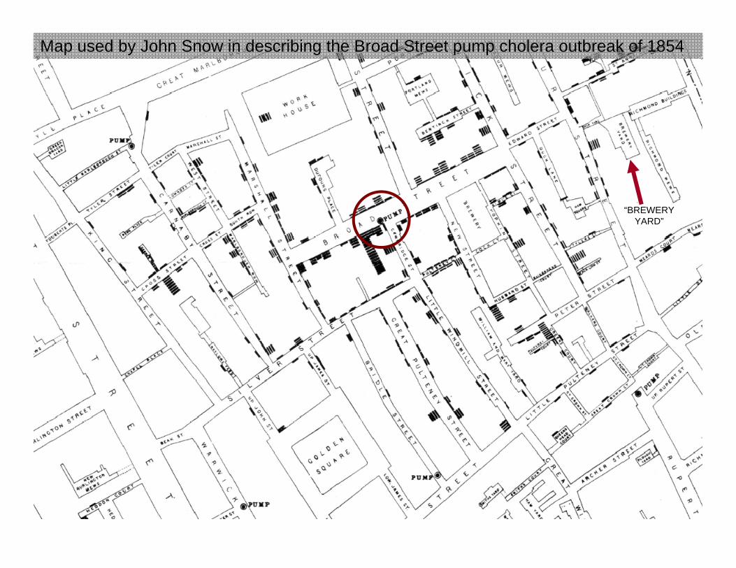
Alcohol outlets: n=1700

0 2.5 51.25 Miles

STARS is a “population-based case-control study”S S s a popu at o based case co t o study

Aschengrau & Seage, Essentials of Epidemiology for Public Health 2003, p. 137 (with edits)

Design of cohort study vs case-control studyS

tudi

es

ctor

Present(exposed)

What % got disease

(risk E)(follow forward in time)

Coh

ort S Fac

Absent(not exposed)

What % got disease

(follow forward in time)

(risk E)

Design of cohort study vs case-control study

Case-Control Studies

Disease

Present(cases)

Absent(controls)

(l k b k d

What % had What % had

(look backwardin time)

been exposed been exposed

Design of cohort study vs case-control study

Case-Control StudiesCohort study RR = A/A+B

C/C+D

Disease

Case-control OR = ADstudy BC

Present(cases)

Absent(controls)

Stu

dies

ctor

Present(exposed) A B

Coh

ort S Fac

Absent(not exposed) DC

Klepeis et al. J Expo Analysis & Environ Epi, 2001

Proportion of time spent in each of six locations

Klepeis et al. J Expo Analysis & Environ Epi, 2001

These are “activity pattern data”

Radon & falloutRadon is a colorless, odorless, naturally occurring, radioactive noble gas that is formed from the decay of radium.

Radon is a significant contaminant that affects indoor air quality worldwide. Radon gas from natural sources can accumulate in buildings, especially inaccumulate in buildings, especially in confined areas such as the basement and reportedly causes 21,000 lung cancer deaths per year in the US.

Radon is the second most frequent cause of lung cancer, after cigarette smoking, and radon‐induced lung cancer i th ht t b th 6th l di fis thought to be the 6th leading cause of cancer death overall. 

Radon can be found in some spring waters and hot springs.

Gatrell & Loytonen, GIS & Health 1998, p.106

RecruitmentRecruitmentCase subjects: HUP and CHOP– Screening by Academic AssociatesScreening by Academic Associates– Interviewing by full-time project staff– Interview takes place in ER, on hospital

ward, home, or research officeward, home, or research office

Control subjects: communityScreening via RDD (random digit dialing)– Screening via RDD (random digit dialing)

– Interviewing by full-time project staff– Interview takes place at home or

research officeresearch office

Time 6:00 am 6:10 6:20 6:30 6:40 6:50 7:00 am

How are you getting around? Here are some examples. Others?

7:00 am 7:10 7:20 7:30 7:40 7:50 8:00 am 8:10 8:20 8:30 8:40 8:50 9:00 am

(1) (2) (3) (4) (5) (6) (7) (0)

What are you doing? Anything else?

(1) (2) (3) (4) (5) (6) (7) (0)

9:10 9:20 9:30 9:40 9:50 10:00 am 10:10 10:20 10:30 10:40 10:50 11:00 am 11:10

(1) (2) (3) (4) (5) (6) (7) (0)

How safe do you feel? On a scale of 1-10, how safe do you feel?

10 FEELING VERY SAFE

1 FEELING VERY UNSAFE

11:10 11:20 11:30 11:40 11:50 12:00 pm 12:10 12:20 12:30 12:40 12:50 1:00 pm 1:10

10 9 8 7 6 5 4 3 2 1

1:20 1:30 1:40 1:50 2:00 pm 2:10 2:20 2:30 2:40 2:50 3:00 pm 3:10 3 20

Are any of these things involved? Anything else?

3:20 3:30 3:40 3:50 4:00 pm 4:10 4:20 4:30 4:40 4:50 5:00 pm 5:10 5:20

(1) (2) (3) (4) (5) (6) (9) (0)

Who are you with? Family, Friends, Girlfriend, Boyfriend, Someone you don’t like, anyone else?

5:20 5:30 5:40 5:50 GO TO NEXT

PAGE

Census tracts: n=381

´ 0 1 20.5 Miles

Time-varying exposures and covariatesTime varying exposures and covariates

4

Yes

0

Expo

sed

No

Y

06 12 18 24

Hours preceding shooting

Figure 1. Dichotomous variable

0.8

1

1.2

e le

vel

H

igh

0

0.2

0.4

0.6

6 12 18 24

Expo

sure

Low

Hours preceding shooting

Figure 3. Gravity measure

Hours preceding shooting

Figure 2. Continuous variable

Neighborhoods: n=69

2

1

´ 0 1 20.5 Miles

Basta, Richmond, WiebeSoc Sci Med 2010

Basta, Richmond, WiebeSoc Sci Med 2010

Median 

Characteristics of one‐day activity paths of 15‐19 year‐old subjects (n=55)

Min Max Mean (SD) (25%, 75%)Time (hrs) spent outside home during one‐day reporting period 0.0 23.5 7.9 (5.6) 8.3 (3.5, 10.9)

Greatest linear distance from home (mi) 0.0 7.2 1.4 (1.7) 0.9 (0.2, 2.4)

Distance travelled (mi) 0.0 20.6 4.5 (4.7) 3.2 (0.7, 9.1)

Time (hrs) spent outside census tract of residence during one‐day reporting period 0.0 19.8 6.3 (5.5) 7.0 (0.0, 9.4)

P ti f t id th h ti th tProportion of outside‐the‐home time that was spent outside census tract of residence (%) 0.0 99.4 71.0 (36.5) 91.5 (56.9, 96.7)

Number of census tracts intersected by subject's y jone‐day activity path 1 34 8.1 (8.5) 6 (1, 10)

25% and 75% denote the twenty‐fifth and seventy‐fifth percentiles, respectively.

In most instances (87.8%), it was one of four types of locations that constituted the place along a subject’s path that was the farthest point (ie, linear distance) from their home: school, work, places of recreation, and food stores and restaurants.

Basta, Richmond, WiebeSoc Sci Med 2010

Median values of the greatest linear distances Interview days

Monday 18%Tuesday 20%Wednesday 6%

gtraveled from home:

1.1 mi on weekdays vs 0.4 mi on weekends (Mann-Whitney z=1.83, p=0.07)

bj t ’ ti iti ll i l d t i l t

y

Wednesday 6%Thursday 11%Friday 15%Saturday 13%

- subjects’ activities generally involved staying closer to home on weekends

Cumulative distances travelled were generallySaturday 13%Sunday 18%

Cumulative distances travelled were generally shorter on weekends also (medians):

4.2 mi on weekdays vs 1.2 mi on weekends(Mann-Whitney z=1.89, p=0.09)

Basta, Richmond, WiebeSoc Sci Med 2010

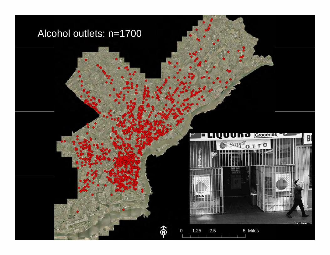
Various measures of exposure to alcohol outlets for 15‐19 year‐old subjects (n=55)

Min Max Mean (SD)Median       

(25%, 75%)l h l l lAlcohol outlet prevalence in 

subject's census tract of residencePer 1000             residents 0.0 46.4 5.1 (8.9) 2.3 (0.8, 4.3)Per road kilometer 0.0 5.2 1.0 (1.0) 0.8 (0.3, 1.1)

Alcohol outlets contacted during one‐day activities

Walked within 18 meters 0 54 3.2 (7.8) 1 (0, 3)

Walked within 200 meters 0 120 12.1 (19.0) 5 (2, 16)

d d h f f h d f f h l l25% and 75% denote the twenty‐fifth and seventy‐fifth percentiles, respectively.

Basta, Richmond, WiebeSoc Sci Med 2010

00

200

s)Spearman’s rho=0.06

p=0.660

150

ed (1

8 m

eter

s0

10ut

lets

con

tact

e0

50Ou

0

0 10 20 30 40 50Outlets per 1000 residents in subject's home census tract

Relation between alcohol outlet prevalence in subjects’ census tracts of                    residence and alcohol outlets contacted during one‐day activities

100

Experiences in their neighborhoods: 13‐17 controls vs. case subjects*

70

80

90p<0.05

40

50

60

70

Perc

ent

Shot

Control

p<0.05

10

20

30

40 p<0.05

0

10

I've heardgunshots

I've seenpeople using or

selling drugs

I often seedrunk people on

the street

I've seensomeone get

stabbed

I've seensomeone pull a

gun on

I've seensomeone get

shotg g gsomebody

*Partial data; preliminary

Wiebe AJPH 2010K02 AA017974

KEY POINTSThe notion that exposure levels can vary in meaningful ways over the course of dailyThe notion that exposure levels can vary in meaningful ways over the course of daily activities has been noted in some research fields, but may remain under-appreciated in large-scale studies of neighborhoods and health.

These results illustrate how individuals’ daily activities frequently occur in locations f th i h d i i t ti b d i d lik l lt iaway from their homes, cross administrative boundaries, and likely result in exposure

to environmental exposures at very different levels than at their home.

Measuring exposure should thus be carefully considered in light of the exposure-disease relation under study and the induction period of the exposure of interest.disease relation under study and the induction period of the exposure of interest.

CONCLUSIONIn studies of environmental exposures that are encountered outside the home and that vary in etiologically meaningful ways over the course of daily activitiesthat vary in etiologically meaningful ways over the course of daily activities, classifying subjects as exposed based solely on the prevalence of the exposure in the administrative geographic unit of their residence (e.g. a Census tract or ZIP code) will likely result in exposure misclassification.

Ask, Where do subjects spend time? And how much time do they spend there? Both will be key to better understanding “neighborhood.”do they spend there? Both will be key to better understanding neighborhood.