Embed Size (px)
Citation preview

MEASURING&
MONITORING
Plant Populations
AUTHORS:
Caryl L. Elzinga Ph.D.Alderspring Ecological ConsultingP.O. Box 64Tendoy, ID 83468
Daniel W. SalzerCoordinator of Research and MonitoringThe Nature Conservancy of Oregon821 S.E. 14th AvenuePortland, OR 97214
John W. WilloughbyState BotanistBureau of Land ManagementCalifornia State Office2135 Butano DriveSacramento, CA 95825
This technical reference represents a team effort by the three authors. The orderof authors is alphabetical and does not represent the level of contribution.
Though this document was produced through an interagency effort, the following BLM numbershave been assigned for tracking and administrative purposes:
BLM Technical Reference 1730-1
BLM/RS/ST-98/005+1730

61
MEASURING AND MONITORING PLANT POPULATIONS
CHAPTER 5. Basic Principles of Sampling
CHAPTER 5. Basic Principles ofSampling
A. IntroductionWhat is sampling? A review of several dictionary definitions led to the following compositedefinition:
The act or process of selecting a part of something with the intent of showing the quality,style, or nature of the whole.
Monitoring does not always involve sampling techniques. Sometimes you can count or measure allindividuals within a population of interest. Other times you may select qualitative techniques thatare not intended to show the quality, style, or nature of the whole population (e.g., subjectivelypositioned photoplots).
What about those situations where you have an interest in learning something about the entirepopulation, but where counting or measuring all individuals is not practical? This situation callsfor sampling. The role of sampling is to provide information about the population in such a waythat inferences about the total population can be made. This inference is the process of general-izing to the population from the sample, usually with the inclusion of some measure of the"goodness" of the generalization (McCall 1982).
Sampling will not only reduce the amount of work and cost associated with characterizing apopulation, but sampling can also increase the accuracy of the data gathered. Some kinds oferrors are inherent in all data collection procedures, and by focusing on a smaller fraction of thepopulation, more attention can be directed toward improving the accuracy of the data collected.
This chapter includes information on basic principles of sampling. Commonly used samplingterminology is defined and the principal concepts of sampling are described and illustrated. Eventhough the examples used in this chapter are based on counts of plants in quadrats (densitymeasurements), most of the concepts apply to all kinds of sampling.
B. Populations and SamplesThe term "population" has both a biological definition and a statistical definition. In this chapterand in Chapter 7, we will be using the term "population" to refer to the statistical population orthe "sampling universe" in which monitoring takes place. The statistical population will some-times include the entire biological population, and other times, some portion of the biologicalpopulation. The population consists of the complete set of individual objects about which youwant to make inferences. We will refer to these individual objects as sampling units. The samplingunits can be individual plants or they may be quadrats (plots), points, or transects. The sample issimply part of the population, a subset of the total possible number of sampling units. Theseterms can be clarified in reference to an artificial plant population shown in Figure 5.1. Thereare a total of 400 plants in this population, distributed in 20 patches of 20 plants each. All theplants are contained within the boundaries of a 20m x 20m "macroplot." The collection of plantsin this macroplot population will be referred to as the "400-plant population." A randomarrangement of ten 2m x 2m quadrats positioned within the 400-plant population is shown in

MEASURING AND MONITORING PLANT POPULATIONS
62 CHAPTER 5. Basic Principles of Sampling
Figure 5.1. Counts of plants within the individual quadrats are directed at the objective ofestimating the total number of plants in the 20m x 20m macroplot. The sampling unit in thiscase is the 2m x 2m quadrat. The sample shown in Figure 5.1 is a set of 10 randomly selectedquadrats. The population in this case is the total collection of all possible 2m x 2m quadratsthat could be placed in the macroplot (N=100).
C. Population Parameters vs. Sample StatisticsPopulation parameters are descriptive measures which characterize the population and areassumed to be fixed but unknown quantities that change only if the population changes. Greekletters such as µ and σ are often used to denote parameters. If we count all the plants in all thequadrats that make up the 400-plant population shown in Figure 5.1 (400 plants), and divide bythe total number of possible 2m x 2m quadrat locations in the macroplot (100 quadrats), weobtain the true average number of plants per quadrat (4 plants/quadrat). This, assuming we havemade no errors, is the true population mean (µ). If we know how much each individual quadratdiffers from the true population mean, we can calculate another important population parame-ter, the true population standard deviation (σ). The standard deviation is a measure of how similareach individual observation is to the overall mean and is the most common measure of variabilityused in statistics. Populations with a large amount of variation among possible sampling unitswill have a larger standard deviation than populations with sampling units that are more similarto one another.
Sample statistics are descriptive measures derived from a sample (e.g., 10 of the possible 100 2mx 2m quadrats). Sample statistics provide estimates of population parameters. Sample statisticswill vary from sample to sample in addition to changing whenever the underlying populationchanges. Roman letters such asX and s are usually used for sample statistics. Consider the
00
2
4
6
8
10
12
14
16
18
20Population parametersTotal population size:400 plantsMean # plants/quadrat:µ = 4Standard deviation:o = 5.005
Sample statistics (n = 10)Mean # plants/quadrat:x = 5.0Standard deviation:s = 6.146
Population estimateEstimated populationsize = 500 plants95% confidenceinterval = ± 361 plants
Sample informationCoordinatesX Y2 2 46 4 016 4 312 6 214 6 56 8 100 12 02 12 614 12 02 14 20
# ofplants
2 4 6 8 10meters
12 14 16 18 20
FIGURE 5.1. Population of 400 plants distributed in 20 clumps of 20 plants. This figure shows a simple random sample often 2m x 2m quadrats, along with sample statistics and true population parameters.
63
MEASURING AND MONITORING PLANT POPULATIONS
CHAPTER 5. Basic Principles of Sampling
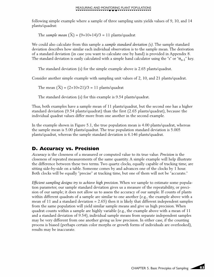
following simple example where a sample of three sampling units yields values of 9, 10, and 14plants/quadrat:
The sample mean (X) = (9+10+14)/3 = 11 plants/quadrat
We could also calculate from this sample a sample standard deviation (s). The sample standarddeviation describes how similar each individual observation is to the sample mean. The derivationof a standard deviation (in case you want to calculate one by hand) is provided in Appendix 8.The standard deviation is easily calculated with a simple hand calculator using the "s" or "σn-1" key.
The standard deviation (s) for the simple example above is 2.65 plants/quadrat.
Consider another simple example with sampling unit values of 2, 10, and 21 plants/quadrat.
The mean (X) = (2+10+21)/3 = 11 plants/quadrat
The standard deviation (s) for this example is 9.54 plants/quadrat.
Thus, both examples have a sample mean of 11 plants/quadrat, but the second one has a higherstandard deviation (9.54 plants/quadrat) than the first (2.65 plants/quadrat), because theindividual quadrat values differ more from one another in the second example.
In the example shown in Figure 5.1, the true population mean is 4.00 plants/quadrat, whereasthe sample mean is 5.00 plants/quadrat. The true population standard deviation is 5.005plants/quadrat, whereas the sample standard deviation is 6.146 plants/quadrat.
D. Accuracy vs. PrecisionAccuracy is the closeness of a measured or computed value to its true value. Precision is thecloseness of repeated measurements of the same quantity. A simple example will help illustratethe difference between these two terms. Two quartz clocks, equally capable of tracking time, aresitting side-by-side on a table. Someone comes by and advances one of the clocks by 1 hour.Both clocks will be equally "precise" at tracking time, but one of them will not be "accurate."
Efficient sampling designs try to achieve high precision. When we sample to estimate some popula-tion parameter, our sample standard deviation gives us a measure of the repeatability, or preci-sion of our sample; it does not allow us to assess the accuracy of our sample. If counts of plantswithin different quadrats of a sample are similar to one another (e.g., the example above with amean of 11 and a standard deviation = 2.65) then it is likely that different independent samplesfrom the same population will yield similar sample means and give us high precision. Whenquadrat counts within a sample are highly variable (e.g., the example above with a mean of 11and a standard deviation of 9.54), individual sample means from separate independent samplesmay be very different from one another giving us low precision. In either case, if the countingprocess is biased (perhaps certain color morphs or growth forms of individuals are overlooked),results may be inaccurate.

MEASURING AND MONITORING PLANT POPULATIONS
64 CHAPTER 5. Basic Principles of Sampling
E. Sampling vs. Nonsampling errorsIn any monitoring study errors should be minimized. Two categories of errors are described next.
1. Sampling errorsSampling errors result from chance; they occur when sample information does not reflect thetrue population information. These errors are introduced by measuring only a subset of allthe sampling units in a population.
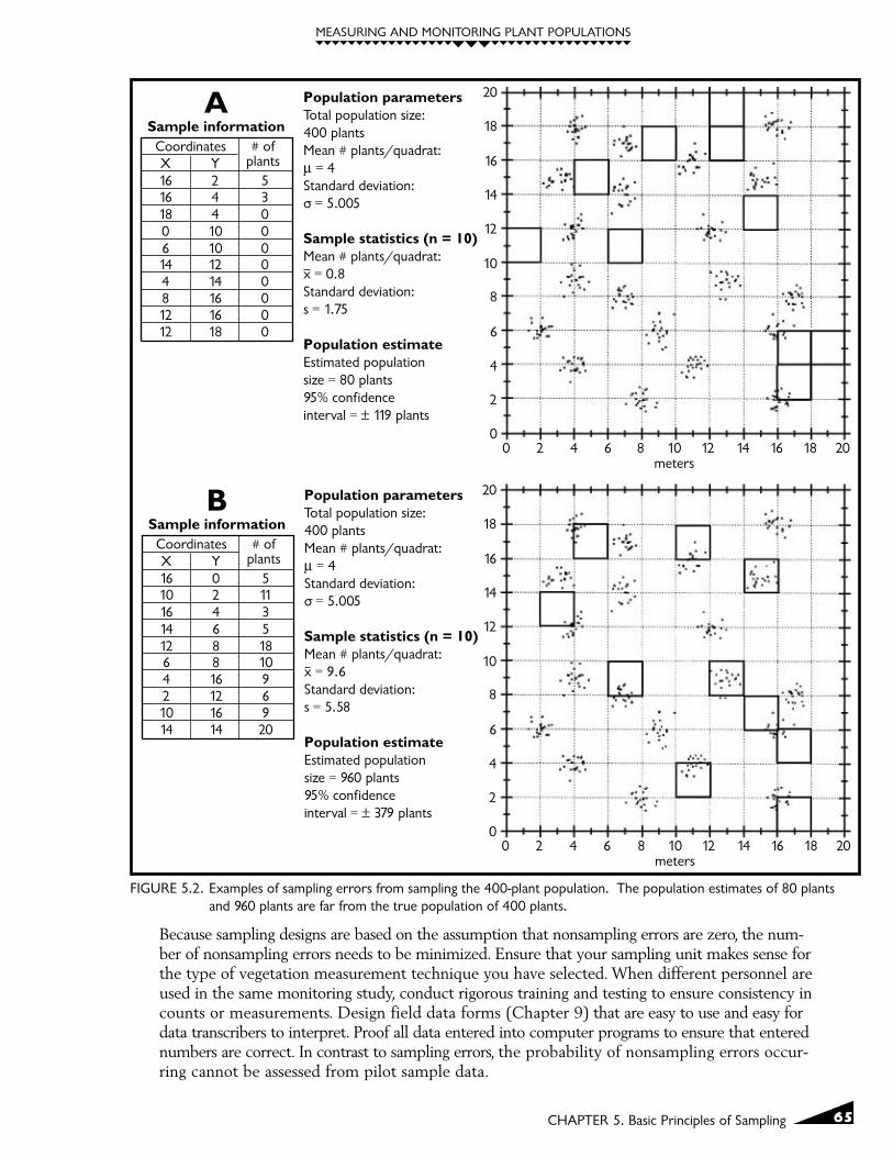
Sampling errors are illustrated in Figure 5.2, in which two separate, completely random sam-ples (2A and 2B) are taken from the 400-plant population shown in Figure 5.1. In each case,ten 2m x 2m quadrats are sampled and an estimate is made of the total number of plantswithin the population. The sample shown in Figure 5.2A produces a population estimate ofonly 80 plants, whereas the sample shown in Figure 5.2B yields an estimate of 960 plants.Both estimates are poor because of sampling error (chance placement of the quadratsresulted in severe under- or overestimates of the true population total).
You can imagine the problems that can arise if you monitor the same population two yearsin a row and get sample information that indicates that the population shifted from 960plants to 80 plants when it really didn't change at all. Sampling errors can lead to two kindsof mistakes: (1) missing real changes (missed-change errors), and (2) detecting apparentchanges that don't really exist (false-change errors).
Sampling errors can be estimated from the sampling data. Some of the basic sampling designtools covered in Chapter 7, enable you to evaluate the effectiveness of your monitoring studyby taking a closer look at the sampling data. This can be especially helpful when setting upnew projects; an evaluation of pilot sampling data can point out potential sampling errorproblems, enabling an investigator to fix them at an early stage of the project. Good samplingdesigns can reduce sampling errors without increasing the cost of sampling.
2. Nonsampling errorsNonsampling errors are errors associated with human, rather than chance, mistakes.Examples of nonsampling errors include:
� Using biased selection rules, such as selecting "representative samples" by subjectivelylocating sampling units, or by substituting sampling units that are "easier" to measure.
� Using vegetation measurement or counting techniques within sampling units in whichattributes cannot be accurately counted or measured. For example, counts of grass stemswithin a quadrat with counts in the hundreds may lead to numerous counting errors.
� Inconsistent field sampling effort. Nonsampling errors can be introduced if different inves-tigators use different levels of effort (e.g., one investigator makes counts from "eye-level,"whereas another counts by kneeling next to the quadrat).
� Transcription and recording errors. Nonsampling errors can be introduced if the datarecorder's "7's" look like "1's" to the person entering the data.
� Incorrect or inconsistent species identification. This category also includes biases introducedby missing certain size classes or color morphs.
65
MEASURING AND MONITORING PLANT POPULATIONS
CHAPTER 5. Basic Principles of Sampling
Because sampling designs are based on the assumption that nonsampling errors are zero, the num-ber of nonsampling errors needs to be minimized. Ensure that your sampling unit makes sense forthe type of vegetation measurement technique you have selected. When different personnel areused in the same monitoring study, conduct rigorous training and testing to ensure consistency incounts or measurements. Design field data forms (Chapter 9) that are easy to use and easy fordata transcribers to interpret. Proof all data entered into computer programs to ensure that enterednumbers are correct. In contrast to sampling errors, the probability of nonsampling errors occur-ring cannot be assessed from pilot sample data.
00
2
4
6
8
10
12
14
16
18
20Population parametersTotal population size:400 plantsMean # plants/quadrat:µ = 4Standard deviation:o = 5.005
Sample statistics (n = 10)Mean # plants/quadrat:x = 0.8Standard deviation:s = 1.75
Population estimateEstimated populationsize = 80 plants95% confidenceinterval = ± 119 plants
Sample informationCoordinatesX Y16 2 516 4 318 4 00 10 06 10 014 12 04 14 08 16 012 16 012 18 0
# ofplants
2 4 6 8 10meters
12 14 16 18 20
FIGURE 5.2. Examples of sampling errors from sampling the 400-plant population. The population estimates of 80 plantsand 960 plants are far from the true population of 400 plants.
00
2
4
6
8
10
12
14
16
18
20Population parametersTotal population size:400 plantsMean # plants/quadrat:µ = 4Standard deviation:o = 5.005
Sample statistics (n = 10)Mean # plants/quadrat:x = 9.6Standard deviation:s = 5.58
Population estimateEstimated populationsize = 960 plants95% confidenceinterval = ± 379 plants
Sample information
A
BCoordinatesX Y16 0 510 2 1116 4 314 6 512 8 186 8 104 16 92 12 610 16 914 14 20
# ofplants
2 4 6 8 10meters
12 14 16 18 20

MEASURING AND MONITORING PLANT POPULATIONS
66 CHAPTER 5. Basic Principles of Sampling
F. Sampling DistributionsOne way of evaluating the risk of obtaining a sample value that is vastly different than the truevalue (such as population estimates of 80 or 960 plants when the true population is 400 plants)is to sample a population repeatedly and look at the differences among the repeated populationestimates. If almost all the separate, independently derived population estimates are similar, thenyou know you have a good sampling design with high precision. If many of the independentpopulation estimates are not similar, then you know your precision is low.
The 400-plant population can be resampled by erasing the 10 quadrats (as shown in eitherFigure 5.1 or Figure 5.2) and putting 10 more down in new random positions. We can keeprepeating this procedure, each time writing down the sample mean. Plotting the results of a largenumber of individual sample means in a simple histogram graph yields a sampling distribution. Asampling distribution is a distribution of many independently gathered sample statistics (mostoften a distribution of sample means). Under most circumstances, this distribution of samplemeans fits a normal or bell-shaped curve.
A distribution of population size estimates from 10,000 separate random samples using ten 2m x2m quadrats from the 400-plant population is shown in Figure 5.3A. The x-axis shows the rangeof different population estimates, and the y-axis shows the relative and actual frequency of thedifferent population estimates. Think of this as the results of 10,000 different people samplingthe same population on the same day, each one setting out 10 randomly positioned 2m x 2mquadrats (somehow without negatively impacting the population) and coming up with their ownindependent population estimate. The highest population estimate out of the 10,000 separatesamples was 960 plants and the lowest population estimate was zero (four of the 10,000 sam-ples yielded a population estimate of zero). The shape of this distribution indicates the magni-tude of likely sampling errors. Wide distributions could yield population estimates that are "far"from the true population value. A sampling design that led to the type of sampling distributiondepicted in Figure 5.3A would not be useful since few of the estimates approach the true popu-lation size of 400 plants. One of the principal objectives in sampling design is to make the shape ofsampling distributions as narrow as possible.
Fortunately, you do not have to repeatedly sample your population and see how wide your sam-pling distribution is to determine if you need to change anything. There are some simple statisti-cal tools that provide a convenient shortcut for evaluating the precision of your sampling effortfrom a single sample. These tools involve calculating standard errors and confidence intervals toestimate sampling precision levels.
1. Standard errorA standard error is the standard deviation of a large numberof independent sample means. It is a measure of precisionthat you derive from a single sample. The formula forcalculating a standard error is as follows:
To paraphrase the earlier statement regarding an importantobjective of sampling design, one of the principal objectives insampling design is to reduce the size of the standard error.
This formula demonstrates that there are only two ways of minimizing standard errors,either: (1) increase sample size (n), or (2) decrease the standard deviation (s).
Formula for standard error:
Where: SE = Standard errors = Standard deviationn = Sample size
SE =sn

67
MEASURING AND MONITORING PLANT POPULATIONS
CHAPTER 5. Basic Principles of Sampling
� Increase sample size. A new sampling distribution of 10,000 separate random samplesdrawn from our example population is shown in Figure 5.3B. This distribution came fromrandomly drawing samples of twenty 2m x 2m quadrats instead of the ten quadrats used tocreate the sampling distribution in Figure 5.3A. This increase in sample size from 10 to 20provides a 29.3% improvement in precision (as measured by the reduced size of thestandard error).
� Decrease sample standard deviation. Another sampling distribution of 10,000 separaterandom samples drawn from our 400-plant population is shown in Figure 5.3C. Thesampling design used to create this distribution of population estimates is similar to
0.10
0.08
0.12
0.06
0.04
0.02
prop
ortio
n pe
r ba
r
Cou
nt
0.0800 900
0.4m x 10m, n = 20
2m x 2m, n = 20
2m x 2m, n = 10
1000700600500estimated total population
40030020010000
200100
300
500
700
900
1100
400
600
800
1000
1200
0.05
0.04
0.06
0.07
0.08
0.03
0.02
0.01
prop
ortio
n pe
r ba
r
Cou
nt
0.0800 900 1000700600500
estimated total population4003002001000
0
200
100
300
500
700
400
600
800
0.05
0.04
0.06
0.03
0.02
0.01
prop
ortio
n pe
r ba
r
Cou
nt
0.0800 900 1000700600500
estimated total population4003002001000
0
200
100
300
500
400
600
A
B
C
FIGURE 5.3. Sampling distributions from three separate sampling designs used on the 400-plantpopulation. All distributions were created by sampling the population 10,000 separatetimes. The smooth lines show a normal bell-shaped curve fit to the data. Figure 3Ashows a sampling distribution where ten 2m x 2m quadrats were used. Figure 3Bshows a sampling distribution where twenty 2m x 2m quadrats were used. Figure 3Cshows a sampling distribution where twenty 0.4m x 10m quadrats were used.

MEASURING AND MONITORING PLANT POPULATIONS
68 CHAPTER 5. Basic Principles of Sampling
the one used to create the sampling distribution in Figure 5.3B. The only differencebetween the two designs is in quadrat shape. The sampling distribution shown in Figure5.3B came from using twenty 2m x 2m quadrats; the sampling distribution shown inFigure 5.3C came from using twenty 0.4m x 10m quadrats. This change in quadrat shapereduced the true population standard deviation from 5.005 plants to 3.551 plants. Thischange in quadrat shape led to a 29.0% improvement in precision over the 2m x 2mdesign shown in Figure 5.3B (as measured by the reduced size of the standard error). This29.0% improvement in precision came without changing the sampling unit size (4m2) orthe number of quadrats sampled (n=20); only the quadrat shape (from square to rectan-gular) changed. When compared to the original sampling design of ten 2m x 2m quadrats,the twenty 0.4m x 10m quadrat design led to a 49.8% improvement in precision. Detailsof this method and other methods of reducing sample standard deviation are covered inChapter 7.
How is the standard error most often used to report the precision level of sampling data?Sometimes the standard error is reported directly. You may see tables with standard errorsreported or graphs that include error bars that show ± 1 standard error. Often, however, thestandard error is multiplied by a coefficient that converts the number into something called aconfidence interval.
2. Confidence intervalsA confidence interval provides an estimate of precision around a sample mean, a sample pro-portion, or an estimate of total population size that specifies the likelihood that the intervalincludes the true value. The vertical lines marked with the "95%" in Figure 5.4 indicate that95% of all the samples (9,500 out of the 10,000) fit between these two lines. Five percent ofthe samples (2.5% in each tail of the distribution) fall outside the vertical lines. These lines
0.05
0.04
0.06
0.07
0.08
0.03
0.02
0.01
prop
ortio
n pe
r ba
r
Cou
nt
0.0800 900 1000700600500
estimated total population400
50%
95%
30020010000
200
100
300
500
400
600
700
800
FIGURE 5.4. Distribution from sampling the 400-plant population 10,000 times using ten samplesof 2m x 2m quadrats. The 95%, 80%, and 50% confidence intervals around the truepopulation of 400 plants are shown. The smooth line shows a normal, bell-shapecurve fit to the data.
80%

69
MEASURING AND MONITORING PLANT POPULATIONS
CHAPTER 5. Basic Principles of Sampling
are positioned equally from the center of the sampling distribution, approximately 320plants away from the center of 400 plants. Thus, 95% of all samples are within ± 320 plantsof the true population size.
A confidence interval includes twocomponents: (1) the confidence inter-val width (e.g., ± 320 plants); and (2)the confidence level (e.g., 90%, 95%).The confidence level indicates theprobability that the interval includesthe true value. Confidence intervalwidth decreases as the confidencelevel decreases. This relationship isshown in Figure 5.4 where three dif-ferent confidence levels are graphedon the sampling distribution obtainedby sampling the 400-plant populationwith ten 2m x 2m quadrats. Thesesame three confidence intervals areshown again in Figure 5.5A, wherethey are graphed in a format com-monly used to report confidenceintervals. There is no gain in precisionassociated with the narrowing of con-fidence interval width as you go fromleft to right in Figure 5.5A (i.e., from95% confidence, to 80% confidence,to 50% confidence); only the proba-bility that the confidence intervalincludes the true value is altered.Another set of three confidence inter-vals is shown in Figure 5.5B. LikeFigure 5.5A, confidence intervals getnarrower as we move from left toright in the graph, but this time theconfidence level is the same (95%)and the narrower widths came fromusing different sampling designs.There is a gain in precision associatedwith the narrowing of confidenceinterval width as you go from left toright in Figure 5.5B (i.e., from the ten2m x 2m design to the twenty 2m x2m design to the twenty 0.4m x 10mdesign) because we have reduced the uncertainty of our population estimate by tighteningthe confidence interval width at the same confidence level.
In order to calculate confidence intervals for sample means, we need two values: (1) the standarderror calculated according to the above formula (SE = s/√n), and (2) the corresponding valuefrom a table of critical values of the t distribution (see Appendix 8 for instructions on calculatingconfidence intervals around proportions). The confidence interval half-width, extending anequal distance on both sides of the mean, is the standard error × the critical t value (except
B
num
ber
of p
lant
s
twenty 2m x 2msampling design
95% confidence levels for 3 different sampling designs
0
200
100
300
500
400
600
700
800
ten 2m x 2m twenty 0.4m x 10m
A
num
ber
of p
lant
s80%
confidence level
different confidence levels for the ten 2m x 2m quadrat design
0
200
100
300
500
400
600
700
800
95% 50%
FIGURE 5.5. Comparison of confidence intervals and confidencelevels for different sampling designs from the 400-plant population. Figure 5A shows three differentconfidence levels (95%, 80%, and 50%) for thesame data set based upon sampling ten 2m x 2mquadrats. Figure 5B shows 95% confidence intervalsfor three different sampling designs that differ inthe level of precision of the population estimates.
MEASURING AND MONITORING PLANT POPULATIONS
70 CHAPTER 5. Basic Principles of Sampling
when sampling from finite populations, see below). The appropriate critical value of tdepends on the level of confidence desired and the number of sampling units (n) in the sam-ple. A table of critical values for the t distribution (Zar 1996) is found in Appendix 5. To usethis table, you must first select the appropriate confidence level column. If you want to be95% confident that your confidence interval includes the true mean, use the column headedα(2) = 0.05. For 90% confidence, use the column headed α(2) = 0.10. You use α(2) becauseyou are interested in a confidence interval on both sides of the mean. You then use the rowindicating the number of degrees of freedom (v), which is the number of sampling unitsminus one (n-1).
For example, if we sample 20 quadrats and come up with a mean of 4.0 plants and a stan-dard deviation of 5.005, here are the steps for calculating a 95% confidence interval aroundour sample mean:
The standard error (SE = s/√n) = 5.005/4.472 = 1.119.
The appropriate t value from Appendix 5 for 19 degrees of freedom (v) is 2.093.
One-half of our confidence interval width is then SE × t-value = 1.119 × 2.093 = 2.342.
Our 95% confidence interval can then be reported as 4.0 ± 2.34 plants/quadrat or we canreport the entire confidence interval width from 1.66 to 6.34 plants/quadrat. This indicates a95% chance that our interval from 1.66 plants/quadrat to 6.34 plants/quadrat includes thetrue value.
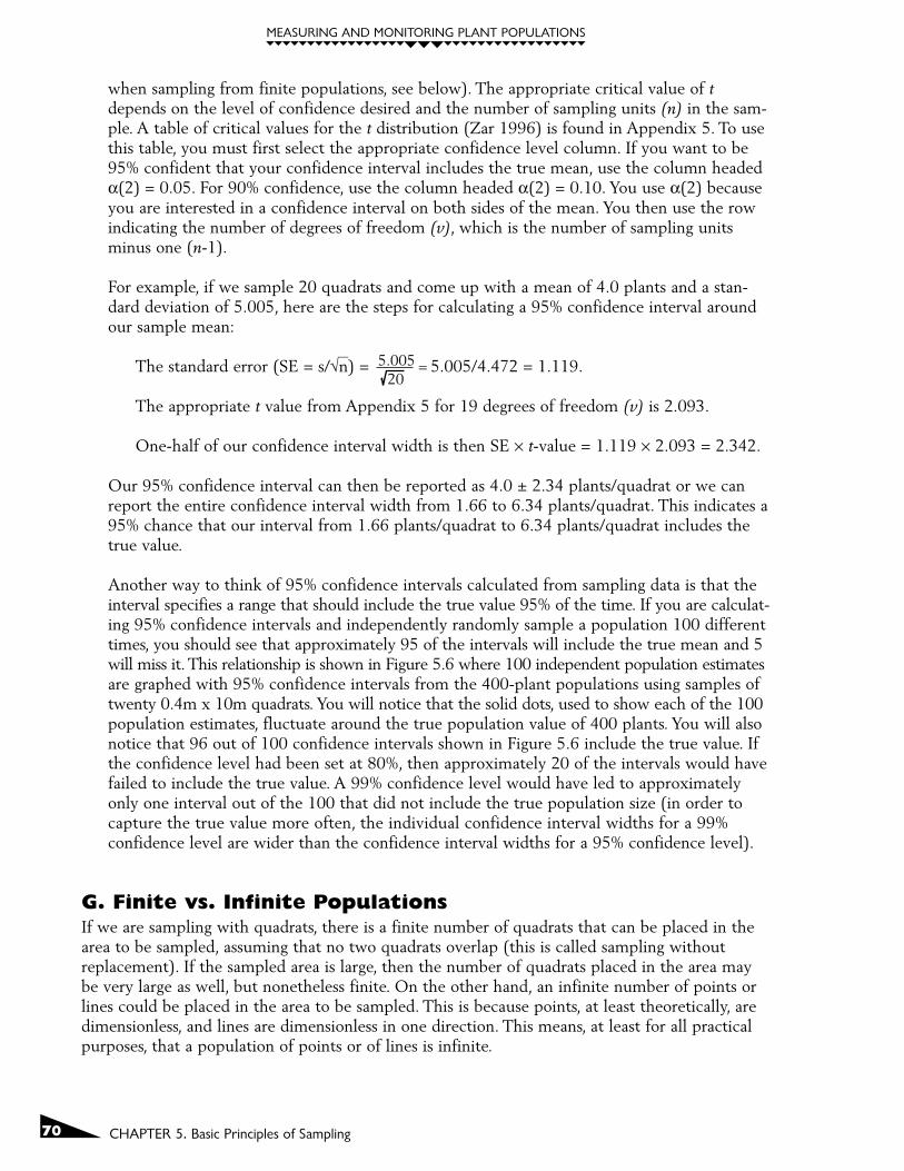
Another way to think of 95% confidence intervals calculated from sampling data is that theinterval specifies a range that should include the true value 95% of the time. If you are calculat-ing 95% confidence intervals and independently randomly sample a population 100 differenttimes, you should see that approximately 95 of the intervals will include the true mean and 5will miss it. This relationship is shown in Figure 5.6 where 100 independent population estimatesare graphed with 95% confidence intervals from the 400-plant populations using samples oftwenty 0.4m x 10m quadrats. You will notice that the solid dots, used to show each of the 100population estimates, fluctuate around the true population value of 400 plants. You will alsonotice that 96 out of 100 confidence intervals shown in Figure 5.6 include the true value. Ifthe confidence level had been set at 80%, then approximately 20 of the intervals would havefailed to include the true value. A 99% confidence level would have led to approximatelyonly one interval out of the 100 that did not include the true population size (in order tocapture the true value more often, the individual confidence interval widths for a 99%confidence level are wider than the confidence interval widths for a 95% confidence level).
G. Finite vs. Infinite PopulationsIf we are sampling with quadrats, there is a finite number of quadrats that can be placed in thearea to be sampled, assuming that no two quadrats overlap (this is called sampling withoutreplacement). If the sampled area is large, then the number of quadrats placed in the area maybe very large as well, but nonetheless finite. On the other hand, an infinite number of points orlines could be placed in the area to be sampled. This is because points, at least theoretically, aredimensionless, and lines are dimensionless in one direction. This means, at least for all practicalpurposes, that a population of points or of lines is infinite.
= 5.005 20
71
MEASURING AND MONITORING PLANT POPULATIONS
CHAPTER 5. Basic Principles of Sampling
If the area to be sampled is large relative to the area that is actually sampled, the distinction betweenfinite and infinite is of only theoretical interest. When, however, the area sampled makes up a signifi-cant portion of the area to be sampled, wecan apply the finite population correction factor,which reduces the size of the standard error.The most commonly used finite populationcorrection factor is shown to the right:
When n is small relative to N, the equationis close to 1, whereas when n is large relative to N, the value approaches zero. The standard error(s/√n) is multiplied by the finite population correction factor to yield a corrected standard errorfor the finite population.
Consider the following example. The density of plant species X is estimated within a 20m x 50mmacroplot (total area = 1000m2). This estimate is obtained by collecting data from randomlyselected 1m x 10m quadrats (10m2). Sampling without replacement, there are 100 possiblequadrat positions.
Thus, our population, N, is 100. Let’s say we take a random sample, n, of 30 of these quadrats andcalculate a mean of eight plants per quadrat and a standard deviation of four plants per quadrat.Our standard error is thus: s/√n = 4/√30 = 0.73. Although our sample mean is an unbiased estimatorof the true population mean and needs no correction, the standard error should be corrected by thefinite population correction factor shown on the top of page 72:
popu
latio
n es
timat
e
50 60 70 80independent samples
0
200
100
300
500
400
600
700
800
0 10 20 30 40 90 100
FIGURE 5.6. Population estimates from 100 separate random samples from the 400-plant population.Each sample represents the population estimate from sampling twenty 0.4m x 10mquadrats. The horizontal line through the graph indicates the true population of 400plants. Vertical bars represent 95% confidence intervals. Four of the intervals miss thetrue population size.
Formula for the finite population correction:
Where: N = total number of potential quadrat positionsn = number of quadrats sampled
FPC = N - nN
total area 1000m2
quadrat area 10m2=

MEASURING AND MONITORING PLANT POPULATIONS
72 CHAPTER 5. Basic Principles of Sampling
Since the standard error is one ofthe factors used to calculate con-fidence intervals (the other is theappropriate value of t from a ttable), correcting the standarderror with the finite populationcorrection factor makes theresulting confidence interval
narrower. It does this, however, only if n is sufficiently large relative to N. A rule of thumb is thatunless the ratio n/N is greater than .05 (i.e., you are sampling more than 5% of the populationarea), there is little to be gained by applying the finite population correction factor to yourstandard error.
The finite population correction factor is also important in sample size determination (Chapter 7)and in adjusting test statistics (Chapter 11). The finite population correction factor works, how-ever, only with finite populations, which we will have when using quadrats, but will not havewhen using points or lines.
H. False-Change Errors and Statistical Power ConsiderationsThese terms relate to situations where two or more sample means or proportions are being com-pared with some statistical test. This comparison may be between two or more places or thesame place between two or more time periods. These terms are pertinent to both planning andinterpretation stages of a monitoringstudy. Consider a simple examplewhere you have sampled a popula-tion in two different years and nowyou want to determine whether achange took place between the twoyears. You usually start with theassumption, called the null hypothe-sis, that no change has taken place.There are two types of decisions thatyou can make when interpreting theresults of a monitoring study: (1) youcan decide that a change took place,or (2) you can decide that no changetook place. In either case, you caneither be right, or you can be wrong (Figure 5.7).
1. The change decision and false-change errors The conclusion that a change took place may lead to some kind of action. For example, if apopulation of a rare plant is thought to have declined, a change in management may beneeded. If a change did not actually occur, this constitutes a false-change error, a sort of falsealarm. Controlling this type of error is important because taking action unnecessarily can beexpensive (e.g., a range permittee is not going to want to change the grazing intensity if adecline in a rare plant population really didn't take place). There will be a certain probabilityof concluding that a change took place even if no difference actually occurred. The probabilityof this occurring is usually labeled the P-value, and it is one of the types of information thatcomes out of a statistical analysis of the data. The P-value reports the likelihood that the
no change hastaken place
monitoring for change — possible errors
there has beena real change
false-change error(Type I)
monitoringsystem detects a
change
no error(Power) 1 -
no error(1 - )
monitoringsystem detects no
change
missed-change error(Type II)
FIGURE 5.7. Four possible outcomes for a statistical test of some nullhypothesis, depending on the true state of nature.
Example of applying the finite population correction factor:
Where: SE' = corrected standard errorSE = uncorrected standard errorN = total number of potential quadrat positionsn = number of quadrats sampled
SE' = (SE) N - nN
SE' = (0.73) = 0.61100 - 30100

73
MEASURING AND MONITORING PLANT POPULATIONS
CHAPTER 5. Basic Principles of Sampling
observed difference was due to chance alone. For example, if a statistical test comparing twosample means yields a P-value of 0.24 this indicates that there is a 24% chance of obtainingthe observed result even if there is no true difference between the two sample means.
Some threshold value for this false-change error rate should be set in advance so that theP-value from a statistical test can be evaluated relative to the threshold. P-values from astatistical test that are smaller than or equal to the threshold are considered statistically"significant," whereas P-values that are larger than the threshold are considered statistically"nonsignificant." Statistically significant differences may or may not be ecologically significantdepending upon the magnitude of difference between the two values. The most commonlycited threshold for false-change errors is the 0.05 level; however, there is no reason to arbi-trarily adopt the 0.05 level as the appropriate threshold. The decision of what false-changeerror threshold to set depends upon the relative costs of making this type of mistake and theimpact of this error level on the other type of mistake, a missed-change error (see below).
2. The no-change decision, missed-change errors, and statistical powerThe conclusion that no change took place usually does not lead to changes in managementpractices. Failing to detect a true change constitutes a missed-change error. Controlling thistype of error is important because failing to take action when a true change actually occurredmay lead to the serious decline of a rare plant population.
Statistical power is the complement of the missed-change error rate (e.g., a missed-changeerror rate of 0.25 gives you a power of 0.75; a missed-change error rate of 0.05 gives you apower of 0.95). High power (a value close to 1), is desirable and corresponds to a low risk ofa missed-change error. Low power (a value close to 0) is not desirable because it correspondsto a high risk of a missed-change error.
Since power levels are directly related to missed-change error levels, either level can bereported and the other level can be easily calculated. Power levels are often reported insteadof missed-change error levels, because it seems easier to convey this concept in terms of thecertainty of detecting real changes. For example, the statement "I want to be at least 90%certain of detecting a real change of five plants/quadrat" (power is 0.90) is simpler to under-stand than the statement "I want the probability of missing a real change of five plants/quadratto be 10% or less" (missed-change error rate is 0.10).
An assessment of statistical power or missed-change errors has been virtually ignored in thefield of environmental monitoring. A survey of over 400 papers in fisheries and aquatic sci-ences found that 98% of the articles that reported nonsignificant results failed to report anypower results (Peterman 1990). A separate survey, reviewing toxicology literature, found highpower in only 19 out of 668 reports that failed to reject the null hypothesis (Hayes 1987).Similar surveys in other fields such as psychology or education have turned up "depressinglylow" levels of power (Brewer 1972; Cohen 1988).
3. Minimum detectable changeAnother sampling design concept that is directly related to statistical power and false-changeerror rates is the size of the change that you want to be able to detect. This will be referredto as the minimum detectable change or MDC. The MDC greatly influences power levels. Aparticular sampling design will be more likely to detect a true large change (i.e., with highpower) than to detect a true small change (i.e., with low power).

MEASURING AND MONITORING PLANT POPULATIONS
74 CHAPTER 5. Basic Principles of Sampling
Setting the MDC requires the consideration of ecological information for the species beingmonitored. How large of a change should be considered biologically meaningful? With alarge enough sample size, statistically significant changes can be detected for changes thathave no biological significance. For example, if an intensive monitoring design leads to theconclusion that the mean density of a plant population increased from 10.0 plants/m2 to10.1 plants/m2, does this represent some biologically meaningful change in populationdensity? Probably not.
Setting a reasonable MDC can be difficult when little is known about the natural history of aparticular plant species. Should a 30% change in the mean density of a rare plant populationbe cause for alarm? What about a 20% change or a 10% change? The MDC considerationsare likely to vary when assessing vegetation attributes other than density, such as cover orfrequency (Chapter 8). The initial MDC, set during the design of a new monitoring study,can be modified once monitoring information demonstrates the size and rate of populationfluctuations.
4. How to achieve high statistical powerStatistical power is related to four separate sampling design components by the followingfunction equation:
Power = a function of (s, n, MDC, and α)
where: s = standard deviationn = number of sampling units
MDC = minimum detectable change α = false-change error rate
Power can be increased in the following four ways:
1. Reducing standard deviation. This means altering the sampling design to reduce theamount of variation among sampling units (see Chapter 7).
2. Increasing the number of sampling units sampled. This method of increasing power isstraightforward, but keep in mind that increasing n has less of an effect than decreasing ssince the square root of sample size is used in the standard error equation (SE = s/√n).
3. Increasing the acceptable level of false-change errors (α).
4. Increasing the MDC.
Note that the first two ways of increasing power are related to making changes in thesampling design, whereas the other two ways are related to making changes in the samplingobjective (see Chapter 6).
5. Graphical comparisonsAs stated, power is driven by four different factors: standard deviation, sample size, mini-mum detectable change size, and false-change error rate. In this section we take a graphicallook at how altering these factors changes power. The comparisons in this section are basedupon sampling a fictitious plant population where we are interested in assessing plant densityrelative to an established threshold value of 25 plants/m2. Any true population densities less
75
MEASURING AND MONITORING PLANT POPULATIONS
CHAPTER 5. Basic Principles of Sampling
than 25 plants/m2 will trigger management action. We are only concerned with the questionof whether the density is lower than 25 plants/m2 and not whether the density is higher. Inthis example, our null hypothesis (HO) is that the population density equals 25 plants/m2 andour alternative hypothesis is that density is less than 25 plants/m2. The density value of 25plants/m2 is the most critical single density value since it defines the lower limit of acceptableplant density.
The figures in this section are all based upon sampling distributions where we happen toknow the true plant density. Recall that a sampling distribution is a bell-shaped curve thatdepicts the distribution of a large number of independently gathered sample statistics. Asampling distribution defines the range and relative probability of any possible sample mean.You are more likely to obtain sample means near the middle of the distribution than you areto obtain sample means near either tail of the distribution.
A sampling distribution based on sampling our fictitious population with a true mean densi-ty of 25 plants/m2 is shown in Figure 5.8A. This distribution is based on a sampling designusing thirty 1m x 1m quadrats where the true standard deviation is ± 20 plants/quadrat. If1,000 different people randomly sample and calculate a sample mean based upon their 30quadrat values, approximately half the individually drawn sample means will be less than 25plants/m2 and half will be greater than 25 plants/m2. Approximately 40% of the samples willyield sample means less than or equal to 24 plants/m2. A few of our 1,000 individuals willobtain estimates of the mean density that deviate from the true value by a large margin. Oneof the individuals will likely stand up and say, "my estimate of the mean density is 13plants/m2", even though the true density is actually 25 plants/m2. As interpreters of themonitoring information, we would conclude that since 999 of the 1,000 people obtainedestimates of the density that were greater than 13, the true density is probably not 13. Ourbest estimate of the true mean density will be the average of the 1,000 separate estimates(this average is likely to be extremely close to the actual true value).
Now that we have the benefit of 1,000 independent estimates of the true mean density, wecan return to the population at a later time, take a single random sample of thirty 1m x 1mquadrats, calculate the sample mean, and then ask the question, "what is the probability ofobtaining our sample mean value if the true population is still 25 plants/m2?" If our samplemean density turns out to be 24 plants/m2, would this lead to the conclusion that the popu-lation has crossed our threshold value? Seeing that our sample mean is lower than our targetvalue might raise some concerns, but we have no objective basis to conclude that the truepopulation is not, in fact, still actually 25 plants/m2. We learned in the previous paragraphthat a full 40% of possible samples are likely to yield mean densities of 24 plants/m2 or less ifthe true mean is 25 plants/m2. Thus, the probability of obtaining a single sample mean of 24plants/m2 or less when the true density is actually 25 plants/m2 is approximately 0.40.Obtaining a sample mean of 24 plants/m2 is consistent with the hypothesis that the truepopulation density is actually 25 plants/m2.
How small a sample mean do we need to obtain to feel confident that the population hasindeed dropped below 25 plants/m2? What will our interpretation be if we obtained a sam-ple mean of 22 plants/m2? Based upon our sampling distribution from the 1,000 people, theprobability of obtaining an estimate of 22 plants/m2 or less is around 20%, which representsa 1-in-5 chance that the true mean is still actually 25 plants/m2. Based upon the samplingdistribution from our 1,000 separate samplers, we can look at the likelihood of obtainingother different sample means. The probability of obtaining a sample of 20 plants/m2 is 8.5%,
MEASURING AND MONITORING PLANT POPULATIONS
76 CHAPTER 5. Basic Principles of Sampling
and the probability of obtaining a sample of 18 plants/m2 is 2.9% if the true mean density is25 plants/m2.
Since in most circumstances we will only have the results from a single sample (and not thebenefit of 1,000 independently gathered sample means), another technique must be used todetermine whether the population density has dropped below 25 plants/m2. One method isto run a statistical test that compares our sample mean to our density threshold value (25
00
5 10 15 20 25
if H0 is true and the true mean = 25
rela
tive
freq
uenc
y
18.830 35 40
A
= 0.62
= 0.05
observed mean density (plants/m2)
00
5 10 15 20 25
rela
tive
freq
uenc
y
18.830 35 40
B
observed mean density (plants/m2)
power = 0.38
if H0 is false and the true mean = 20
reject H0 do not reject H0
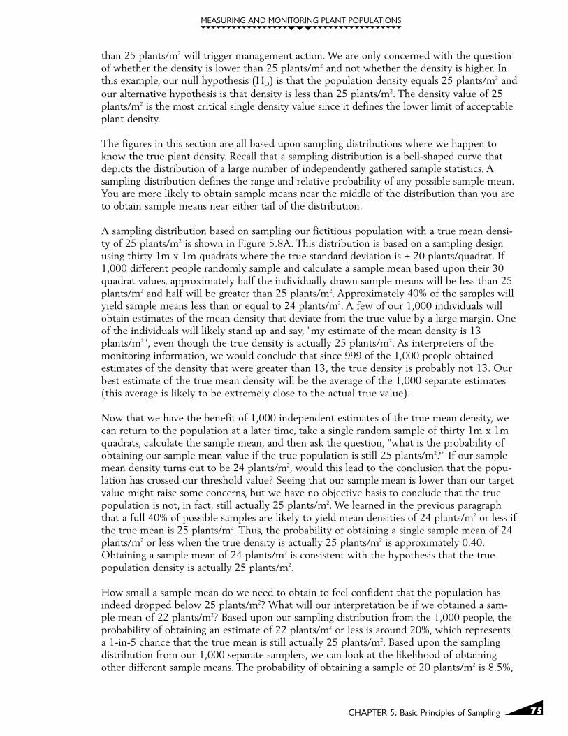
FIGURE 5.8. Example of sampling distributions for mean plant density in samples of 30 permanentquadrats where the among-quadrat standard deviation is 20 plants/m2. Part A is thesampling distribution for the case in which the null hypothesis, H0, is true and the truepopulation mean density is 25 plants/m2. The shaded area in part A is the criticalregion for = 0.05 and the vertical dashed line is at the critical sample mean value, 18.8.Part B is the sampling distribution for the case in which the H0 is false and the true meanis 20 plants/m2. In both distributions, a sample mean to the left of the vertical dashedline would reject H0, and to the right of it, would not reject H0. Power and values inpart B, in which H0 is false and the true mean = 20, are the proportion of samplemeans that would occur in the region in which H0 was rejected or not rejected,respectively (adapted from Peterman 1990).

77
MEASURING AND MONITORING PLANT POPULATIONS
CHAPTER 5. Basic Principles of Sampling
plants/m2). The statistical test will yield a P-value that defines the probability of obtainingour sample mean if the true population density is actually 25 plants/m2. As interpreters ofour monitoring information, we will need to set some probability threshold P-value to guideour interpretation of the results from the statistical test. This P-value threshold defines ouracceptable false-change error rate. If we run a statistical test that compares our sample meanto our density threshold value (25 plants/m2) and the P-value from the test is lower than ourthreshold value, then we conclude that the population density has, in fact, declined below 25plants/m2. Thus, if we set our P-value threshold to 0.05 and the statistical test yields a P-value of 0.40, then we fail to reject the null hypothesis that the true population density is 25plants/m2. If, however, the statistical test yields a P-value of 0.022, this is lower than ourthreshold P-value of 0.05, and we would reject the null hypothesis that the population is 25plants/m2 in favor of our alternative hypothesis that the density is lower than 25 plants/m2.
The relationship between the P-value threshold of 0.05 and our sampling distribution basedupon sampling thirty 1m x 1m quadrats is shown in Figure 5.8A. The threshold density valuecorresponding to our P-value threshold of 0.05 is 18.8 plants/m2, which is indicated on thesampling distribution by the dashed vertical line. Thus, if we obtain a mean density of 18plants/m2, which is to the left of the vertical line, we reject the null hypothesis that thepopulation density is 25 plants/m2 in favor of an alternative hypothesis that density is lowerthan 25 plants/m2. If we obtain a mean density of 21 plants/m2, which is to the right of thevertical line, then we fail to reject the null hypothesis that the population density is really 25plants/m2.
So far we have been discussing the situation where the true population density is right at thethreshold density of 25 plants/m2. Let's look now at a situation where we know the truedensity has declined to 20 plants/m2. What is the likelihood of our detecting this true densitydifference of 5 plants/m2? Figure 5.8B shows a new sampling distribution based upon thetrue density of 20 plants/m2 (standard deviation is still ± 20 plants/m2). We know from ourprevious discussion that sample means to the right of the vertical line in Figure 5.8A lead tothe conclusion that we can't reject the null hypothesis that our density is 25 plants/m2. If ournew sample mean turns out to exactly match the new true population mean (i.e., 20plants/m2), will we reject the idea that the sample actually came from a population with atrue mean of 25 plants/m2? No, at least not at our stated P-value (false-change error) thresh-old of 0.05. A sample mean value of 20 plants/m2 falls to the right of our dashed thresholdline in the "do not reject HO" portion of the graph and we would have failed to detect thetrue difference that actually occurred. Thus, we would have committed a missed-change error.
What is the probability of missing the true difference of five plants/m2 show in Figure 5.8B?This probability represents the missed-change error rate (β) and it is defined by the nonshadedarea under the sampling distribution in Figure 5.8B, which represents 62% of the possiblesample mean values. Recall that the area under the whole curve defines the entire range ofpossible values that you could obtain by sampling the population with the true mean = 20plants/m2. If we bring back our 1,000 sampling people and have each of them sample thirty1m x 1m quadrats in our new population, we will find that approximately 620 of them willobtain estimates of the mean density that are greater than the 18.8 plants/m2 threshold valuethat is shown by the vertical dashed line. What about the other 380 people? They will obtainpopulation estimates fewer than the critical threshold of 18.8 plants/m2 and they will rejectthe null hypothesis that the population equals 25 plants per quadrat. This proportion of 0.38(380 people out of 1,000 people sampling) represents the statistical power of our samplingdesign and it is represented by the shaded area under the curve in Figure 5.8B. If the truepopulation mean is indeed 20 plants/m2 instead of 25 plants/m2, then we can be 38%

MEASURING AND MONITORING PLANT POPULATIONS
78 CHAPTER 5. Basic Principles of Sampling
(power = 0.38) sure that we will detect this true difference of five plants/m2. With this par-ticular sampling design (thirty 1m x 1m quadrats) and a false-change error rate of α=0.05,we run a 62% chance (β=0.62) that we will commit a missed-change error (i.e., fail to detectthe true difference of five plants/m2). If the difference of five plants/m2 is biologically impor-tant, a power of only 0.38 would not be satisfactory.
We can improve the low-power situation in four different ways: (1) increase the acceptablefalse-change error rate; (2) increase the acceptable MDC; (3) increase sample size; or (4)decrease the standard deviation. New paired sampling distributions illustrate the influence ofmaking each of these changes.
a. Increasing the acceptable false-change error rate
In Figure 5.8B, a false-change error rate of α=0.05 resulted in a missed-change error rate ofβ=0.62 to detect a difference of five plants/m2. Given these error rates, we are more than 12times more likely to commit a missed-change error than we are to commit a false-changeerror. What happens to our missed-change error rate if we specify a new, higher false-changeerror rate? Shifting our false-change error rate from α=0.05 to α=0.10 is illustrated in Figure 5.9
00
5 10 15 25
if H0 is true and the true mean = 25
rela
tive
freq
uenc
y
20.230 35 40
A
= 0.47
observed mean density (plants/m2)
= 0.10
00
5 10 15 20 25
rela
tive
freq
uenc
y
20.230 35 40
B
observed mean density (plants/m2)
power = 0.53
if H0 is false and the true mean = 20
FIGURE 5.9. The critical region for the false-change error in the sampling distributions from Figure5.8 has been increased from = 0.05 to = 0.10. Part B, in which the H0 is false andthe true mean = 20, shows that power is larger for = 0.10 than for Figure 5.8 where = 0.05 (adapted from Peterman 1990).
79
MEASURING AND MONITORING PLANT POPULATIONS
CHAPTER 5. Basic Principles of Sampling
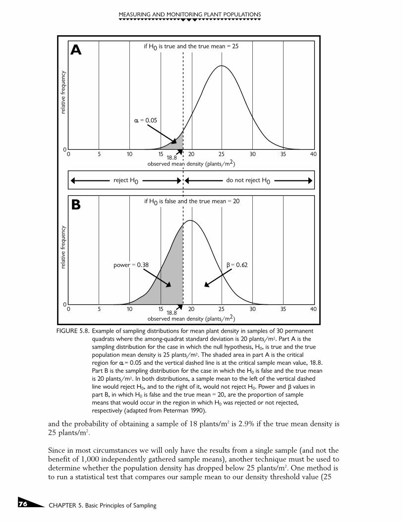
for the same sampling distributions shown in Figure 5.8. Our critical density threshold at theP=0.10 level is now 20.21 plants/m2, and our missed-change error rate has dropped fromβ=0.62 down to β=0.47 (i.e., the power to detect a true five plant/m2 difference went from0.38 to 0.53). A sample mean of 20 plants/m2 will now lead to the correct conclusion that adifference of five plants/m2 between the populations does exist. Of course, the penalty wepay for increasing our false-change error rate is that we are now twice as likely to concludethat a difference exists in situations when there is no true difference and our populationmean is actually 25 plants/m2. Changing the false-change error rate even more, to α=0.20,(Figure 5.10) reduces the probability of making a missed-change error down to β=0.29 (i.e.,giving us a power of 0.71 to detect a true difference of five plants/m2).
b. Increasing the acceptable MDC
Any sampling design is more likely to detect a true large difference than a true small differ-ence. As the magnitude of the difference increases, we will see an increase in the power todetect the difference. This relationship is shown in Figure 5.11B, where we see a samplingdistribution with a true mean density of 15 plants/m2, which is 10 plants/m2 below ourthreshold density of 25 plants/m2. The false-change error rate is set at α=0.05 in this example.
00
5 10 15 20
if H0 is true and the true mean = 25
rela
tive
freq
uenc
y
21.9 30 35 40
FIGURE 5.10. The critical region for the false-change error in the sampling distributions fromFigure 5.8 has been increased from = 0.05 to = 0.20. Part B, in which theH0 is false and the true mean = 20, shows that power is larger for = 0.20 thanfor Figure 5.8 where = 0.05 or Figure 5.9 where = 0.10. Again, a samplemean to the left of the vertical dashed line would reject H0, while one to theright of it would not reject H0 (adapted from Peterman 1990).
A
00
5 10 15 20observed mean density (plants/m2)
rela
tive
freq
uenc
y
21.9 30 35 40
B
= 0.29power = 0.71
= 0.20
if H0 is false and the true mean = 20
observed mean density (plants/m2)

MEASURING AND MONITORING PLANT POPULATIONS
80 CHAPTER 5. Basic Principles of Sampling
This figure shows that the statistical power to detect this larger difference of 10 plants/m2
(25 plants/m2 to 15 plants/m2) is 0.85 compared with the original power value of 0.38 todetect the difference of five plants/m2 (25 plants/m2 to 20 plants/m2). Thus, with a false-change error rate of 0.05, we can be 85% certain of detecting a difference from our 25plants/m2 threshold of 10 plants/m2 or greater. If we raised our false-change error fromα=0.05 to α=0.10 (not shown in Figure 5.11), our power value would rise to 0.92, whichcreates a sampling situation where our two error rates are nearly equal (α=0.10, β=0.08).
c. Increasing the sample size
The sampling distributions shown in Figures 5.8 to 5.11 were all created by sampling thepopulations with n=30 1m x 1m quadrats. Any increase in sample size will lead to a subse-quent increase in power to detect some specified minimum detectable difference. Thisincrease in power results from the sampling distributions becoming narrower. Sampling dis-tributions based on samples of n=50 are shown in Figure 5.12 where the true differencebetween the two populations is once again five plants/m2 with a false-change error ratethreshold of α=0.05. The increase in sample size led to an increase in power from
00
5 10 15 20 25
if H0 is true and the true mean = 25
rela
tive
freq
uenc
y
18.8 30 35 40
FIGURE 5.11. Part A is the same as Figure 5.8; in part B, the true population mean is 15 plants/m2
instead of the 20 plants/m2 shown in Figure 5.8. Note that power increases(and decreases) when the new true population mean gets further from the originaltrue mean of 25 plants/m2. Again, a sample mean to the left of the vertical dashedline would reject H0, while one to the right of it would not reject H0 (adapted fromPeterman 1990).
A
00
5 10 15 20 25observed mean density (plants/m2)
rela
tive
freq
uenc
y
18.8 30 35 40
B
= 0.15power = 0.85
= 0.05
observed mean density (plants/m2)
if H0 is false and the true mean = 15

81
MEASURING AND MONITORING PLANT POPULATIONS
CHAPTER 5. Basic Principles of Sampling
power=0.38 with n=30 to power=0.54 with n=50. Note that the critical threshold densityassociated with an α = 0.05 is now 20.3 plants/m2 as compared to the 18.8 plants/m2
threshold when n = 30.
d. Decreasing the standard deviation
The sampling distributions shown in Figures 5.8 to 5.12 all are based on sampling distributionswith a standard deviation of ±20 plants/m2. The quadrat size used in the sampling was asquare 1m x 1m quadrat. If individuals in the plant population are clumped in distribution,then it is likely that a rectangular shaped quadrat will result in a lower standard deviation(See Chapter 7 for a detailed description of the relationship between standard deviation andsampling unit size and shape). Figure 5.13 shows sampling distributions where the standarddeviation was reduced from ±20 plants/m2 to ±10 plants/m2. Note that the critical thresholddensity associated with an α = 0.05 is now 21.9 plants/m2 as compared to the 18.8 plants/m2
threshold when the standard deviation was ± 20 plants/m2. This reduction in the true stan-dard deviation came from a change in quadrat shape from the 1m x 1m square shape to a0.2m x 5m rectangular shape. Note that quadrat area (1m2) stayed the same so that themean densities are consistent with the previous sampling distributions shown in Figures 5.8
00
5 10 15 25
if H0 is true and the true mean = 25
With n = 50 instead of n = 30
rela
tive
freq
uenc
y
30 35 40
FIGURE 5.12. The sample size was increased to n = 50 quadrats from the n = 30 quadrats shown inFigure 5.8. Note that power increases (and decreases) at larger sample sizes. Again,a sample mean to the left of the vertical dashed line would reject H0, while one to theright of it would not reject H0 (adapted from Peterman 1990).
A
00
5 10 15 20 25observed mean density (plants/m2)
rela
tive
freq
uenc
y
30 35 40
B
power = 0.54 = 0.46
= 0.05
observed mean density (plants/m2)
if H0 is false and the true mean = 20
20 20.3
20.3
MEASURING AND MONITORING PLANT POPULATIONS
82 CHAPTER 5. Basic Principles of Sampling
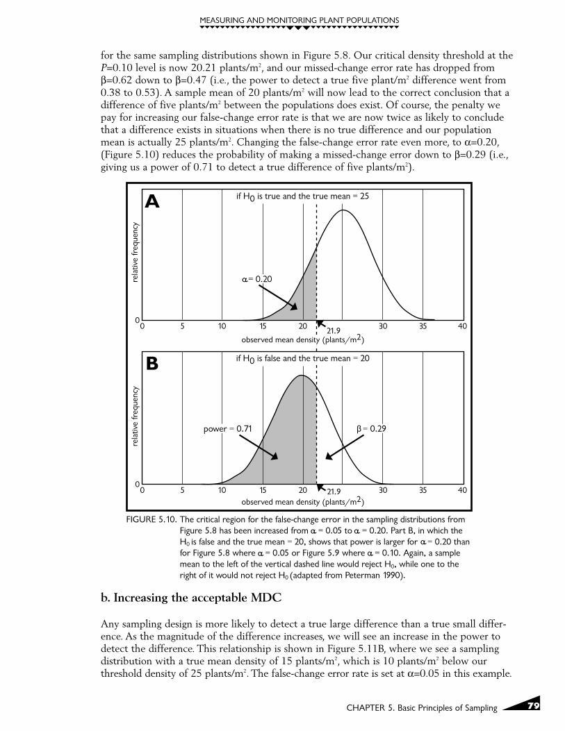
through 5.12. This reduction in standard deviation led to a dramatic improvement in power,from 0.38 (with sd = 20 plants/m2) to 0.85 (with sd = 10 plants/m2). Reducing the standarddeviation has a more direct impact on increasing power than increasing sample size, becausethe sample size is reduced by taking its square root in the standard error equation (SE = s/√n).Recall that the standard error provides an estimate of sampling precision from a single samplewithout having to enlist the support of 1,000 people who gather 1,000 independent samplemeans.
e. Power curves
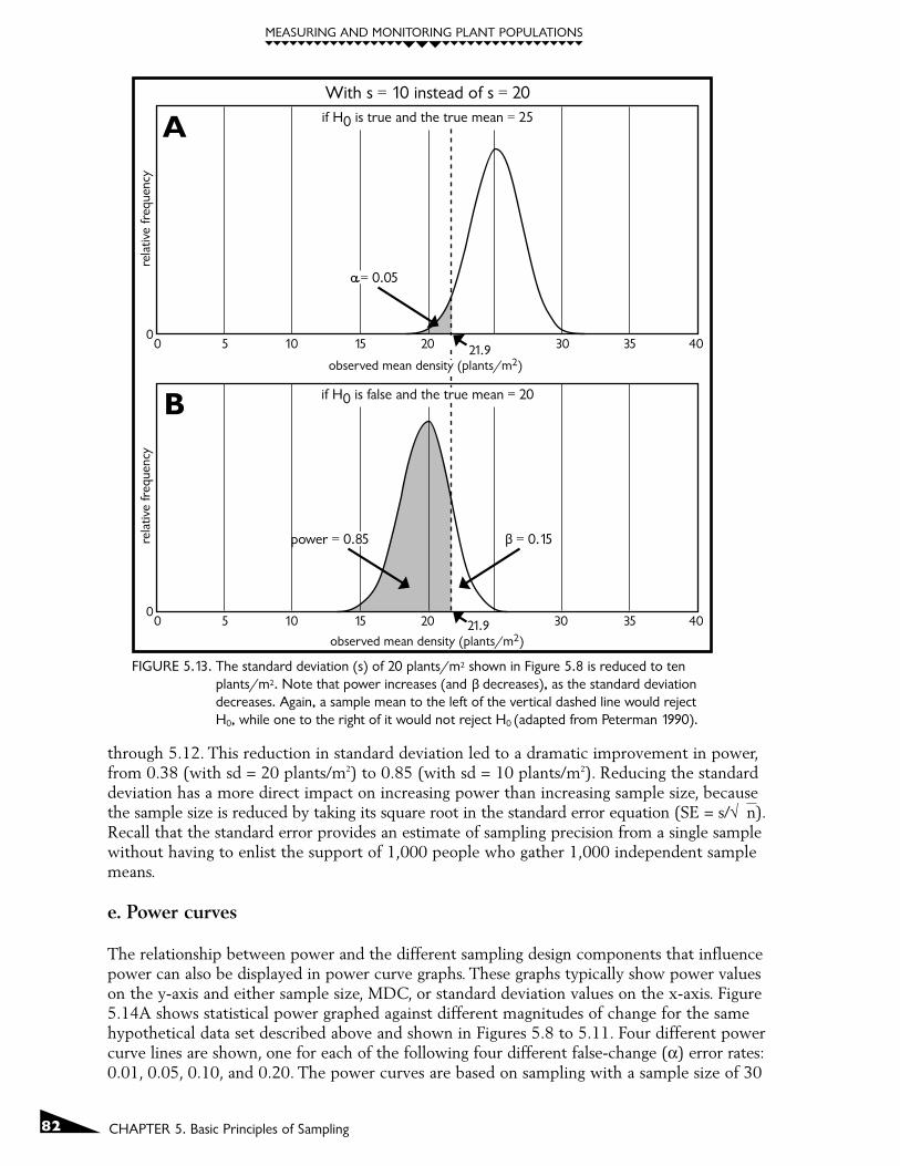
The relationship between power and the different sampling design components that influencepower can also be displayed in power curve graphs. These graphs typically show power valueson the y-axis and either sample size, MDC, or standard deviation values on the x-axis. Figure5.14A shows statistical power graphed against different magnitudes of change for the samehypothetical data set described above and shown in Figures 5.8 to 5.11. Four different powercurve lines are shown, one for each of the following four different false-change (α) error rates:0.01, 0.05, 0.10, and 0.20. The power curves are based on sampling with a sample size of 30
00
5 10 15
if H0 is true and the true mean = 25
With s = 10 instead of s = 20
rela
tive
freq
uenc
y
30 35 40
FIGURE 5.13. The standard deviation (s) of 20 plants/m2 shown in Figure 5.8 is reduced to tenplants/m2. Note that power increases (and decreases), as the standard deviationdecreases. Again, a sample mean to the left of the vertical dashed line would rejectH0, while one to the right of it would not reject H0 (adapted from Peterman 1990).
A
00
5 10 15 20
observed mean density (plants/m2)
rela
tive
freq
uenc
y
30 35 40
B
power = 0.85 = 0.15
= 0.05
observed mean density (plants/m2)
if H0 is false and the true mean = 20
20 21.9
21.9

83
MEASURING AND MONITORING PLANT POPULATIONS
CHAPTER 5. Basic Principles of Sampling
quadrats and a standard deviation of 20 plants/m2. For any particular false-change error rate,power increases as the magnitude of the minimum detectable change increases. When α=0.05,the power to detect small changes is very low (Figure 5.14A). For example, we have only a13% chance of detecting a difference of 2 plants/m2 (i.e., a density of 23 plants/m2 which is 2plants/m2 below our threshold value of 25 plants/m2). In contrast, we can be 90% sure ofdetecting a minimum difference of 11 plants/m2. We can also attain higher power by increasing
0
0.1
0.2
0.3
0.4
0.5
0.6
0.7
0.8
0.9
1
2 3 4 5 6 7 8 9 10 11 12 13 14minimum detectable change size
pow
er
15 16 17 18 19 20
= 0.
20
= 0.
10
= 0.
05
= 0.
01
An = 30sd = 20
0
0.1
0.2
0.3
0.4
0.5
0.6
0.7
0.8
0.9
1
2 3 4 5 6 7 8 9 10 11 12 13 14minimum detectable change size
pow
er
15 16 17 18 19 20
= 0.
20=
0.10
= 0.
05
= 0.
01
Bn = 50sd = 20
FIGURE 5.14. Power curves showing power values for various magnitudes of minimum detectable changeand false-change error rates when the standard deviation is 20. Part A shows power curveswith a sample size of 30. Part B shows power curves with a sample size of 50.

MEASURING AND MONITORING PLANT POPULATIONS
84 CHAPTER 5. Basic Principles of Sampling
the false-change error rate. The power to detect a change of eight plants/m2 is only 0.41when α=0.01, but it increases to 0.69 at α=0.05, to 0.81 at α=0.10, and to 0.91 at α=0.20.
A different set of power curves are shown in Figure 5.14B where the sample size is n=50 insteadof the n=30 shown in Figure 5.14A. This larger smaller sample size shifts all of the power curvesto the left, making it more likely that smaller changes will be detected. For example, with a false-change error rate of α=0.10, the power to detect a seven plant/m2 difference is 0.88 with asample size of n=50 quadrats compared to the power of 0.73 with a sample size of n=30quadrats.
Power curves that show the effect of reducing the standard deviation are shown in Figure5.15. Figure 5.15A is the same as Figure 5.14A where the standard deviation is 20 plants/m2.Figure 5.15B shows the same power curves except they are based on a standard deviation of10 plants/m2. The smaller standard deviation shifts all of the power curves to the left andresults in much steeper slopes. The smaller standard deviation leads to substantially higherpower levels for any particular MDC value. For example, the power to detect a change offive plants/m2 with a false change error rate of α=0.10 is only 0.53 in Figure 5.15A ascompared to the power of 0.92 in Figure 5.15B.
6. Setting false-change and missed-change error ratesBoth false-change and missed-change error rates can be reduced by sampling design changesthat increase sample size or decrease sample standard deviations. Missed-change and false-change error rates are inversely related, which means that reducing one will increase theother (but not proportionately) if no other changes are made. The decision of which type oferror is more important should be based on the nature of the changes you are trying todetermine, and the consequences of making either kind of mistake.
Because false-change and missed-change error rates are inversely related to each other, andbecause these errors have different consequences to different interest groups, there are differ-ent opinions as to what the "acceptable" error rates should be. The following examplesdemonstrate the conflict between false-change and missed-change errors.
� Testing for a lethal disease. When screening a patient for some disease that is lethal with-out treatment, a physician is less concerned about making a false diagnosis error (analogousto a false-change error) of concluding that the person has the disease when they do notthan failing to detect the disease (analogous to a missed-change error) and concluding thatthe person does not have the disease when in fact they do.
� Testing for guilt in our judicial system. In the United States, the null hypothesis is thatthe accused person is innocent. Different standards for making judgement errors are useddepending upon whether the case is a criminal or a civil case. In criminal cases, proof mustbe "beyond a reasonable doubt." In these situations it is less likely that an innocent personwill be convicted (analogous to a false-change error), but it is more likely that a guilty per-son will go free (analogous to a missed-change error). In civil cases, proof only needs to be"on the balance of probabilities." In these situations, there is a greater likelihood of makinga false conviction (analogous to a false-change error), but a lower likelihood of making amissed conviction (analogous to a missed-change) error.
� Testing for pollution problems. In pollution monitoring situations, the industry has aninterest in minimizing false-change errors and may desire a very low false-change error

85
MEASURING AND MONITORING PLANT POPULATIONS
CHAPTER 5. Basic Principles of Sampling
rate (e.g., α = 0.01 or 0.001). Companies do not want to be shut down or implementexpensive pollution control procedures if a real impact has not occurred. In contrast, anorganization concerned with the environmental impacts of some pollution activity willlikely want to have high power (low missed-change error rate) so that they do not missany real changes that take place. They may not be as concerned about occasional false-
0
0.1
0.2
0.3
0.4
0.5
0.6
0.7
0.8
0.9
1
2 3 4 5 6 7 8 9 10 11 12 13 14minimum detectable change
pow
er
15 16 17 18 19 20
An = 30sd = 20
0
0.1
0.2
0.3
0.4
0.5
0.6
0.7
0.8
0.9
1
2 3 4 5 6 7 8 9 10 11 12 13 14minimum detectable change
pow
er
15 16 17 18 19 20
= 0.
20
= 0.
10
= 0.
05
= 0.
01
= 0.
20=
0.10
= 0.
05
= 0.
01
Bn = 30sd = 10
FIGURE 5.15. Power curves showing power values for various magnitudes of minimum detectable changeand false-change error rates when the sample size = 30. Part A shows power curveswith a standard deviation of 20 plants/m2. Part B shows power curves with a standarddeviation of 10 plants/m2.

MEASURING AND MONITORING PLANT POPULATIONS
86 CHAPTER 5. Basic Principles of Sampling
change errors (which would result in additional pollution control efforts even though realchanges did not take place).
Missed-change errors may be as costly or more costly than false-change errors in environ-mental monitoring studies (Toft and Shea 1983; Peterman 1990; Fairweather 1991). A false-change error may lead to the commitment of more time, energy, and people, but probablyonly for the short period of time until the mistake is discovered (Simberloff 1990). In con-trast, a missed-change error, as a result of a poor study design, may lead to a false sense ofsecurity until the extent of the damages are so extreme that they show up in spite of a poorstudy design (Fairweather 1991). In this case, rectifying the situation and returning thesystem to its preimpact condition could be costly. For this reason, you may want to set equalfalse-change and missed-change error rates or even consider setting the missed-change errorrate lower than the false-change error rate (Peterman 1990; Fairweather 1991).
There are many historical examples of costly missed-change errors in environmental moni-toring. For example, many fish population monitoring studies have had low power to detectbiologically meaningful declines so that declines were not detected until it was too late andentire populations crashed (Peterman 1990). Some authors advocate the use of somethingthey call the "precautionary principle" (Peterman and M'Gonigle 1992). They argue that, insituations where there is low power to detect biologically meaningful declines in some envi-ronmental parameter, management actions should be prescribed as if the parameter had actu-ally declined. Similarly, some authors prefer to shift the burden of proof in situations wherethere might be an environmental impact from environmental protection interests to indus-try/development interests (Peterman 1990; Fairweather 1991). They argue that a conservativemanagement strategy of "assume the worst until proven otherwise" should be adopted. Underthis strategy, developments that may negatively impact the environment should not proceeduntil the proponents can demonstrate, with high power, a lack of impact on the environment.
7. Why has statistical power been ignored for so long?It is not clear why missed-change errors, power, and minimum detectable change size havetraditionally been ignored. Perhaps researchers have not been sufficiently exposed to the ideaof missed-change errors. Most introductory texts and statistics courses deal with the materialonly briefly. Computer packages for power analysis have only recently become available.Perhaps people have not realized the potentially high costs associated with making missed-change errors. Perhaps researchers have not understood how understanding power canimprove their work.
The issue of power and missed-change errors has gained a lot of attention in recent years. Aliterature review in the 1980’s would not have turned up many articles dealing with statisticalpower issues. A literature review today would turn up dozens of articles in many disciplinesfrom journals all over the world (see Peterman 1990 and Fairweather 1991 for good reviewpapers on statistical power). Journal editors may soon start requiring that power analysisinformation be reported for all nonsignificant results (Peterman 1990). There may also besome departure from the strict adherence to the 0.05 significance level (Peterman 1990;Fairweather 1991).
8. Use of prior power analysis during study designPower analysis can be useful during both the design of monitoring studies and in the inter-pretation of monitoring results. The former is sometimes called "prior power analysis,"whereas the latter is sometimes called "post-hoc power analysis" (Fairweather 1991). Post-hocpower analysis is covered in Chapter 11.

87
MEASURING AND MONITORING PLANT POPULATIONS
CHAPTER 5. Basic Principles of Sampling
The use of power analysis during the design and planning of monitoring studies providesvaluable information that can help avoid monitoring failures. Once some preliminary or pilotdata have been gathered, or if some previous years' monitoring data are available, poweranalysis can be used to evaluate the adequacy of the sampling design. Prior power analysis canbe done in several different ways. All are based upon the power function described earlier:
Power = a function of (s, n, MDC, and α)
The power of a particular sampling design can be evaluated by plugging sample standarddeviation, sample size, the desired MDC, and an acceptable false-change error rate, intoequations or computer programs (Appendix 16) and solving for power. If the power to detecta biologically important change turns out to be quite low (high probability of a missed-change error), then the sampling design can be modified to try to achieve higher power.
Alternatively, a desired power level can be specified and the terms in the power function canbe rearranged to solve for sample size. This will give you assurance that your study designwill succeed in being able to detect a certain magnitude of change at the specified power andfalse-change error rate. This is the format for the sample size equations that are discussed inChapter 7 and presented in Appendix 7.
Still another way to do prior power analysis is to specify a desired power level and a particu-lar sample size and then rearrange the terms in the power function to solve for the MDC(Rotenberry and Wiens 1985; Cohen 1988). If the MDC is unacceptably large, then attemptsshould be made to improve the sampling design. If these efforts fail, then the decision mustbe made to either live with the large MDC or to reject the sampling design and perhapsconsider an alternative monitoring approach.
The main advantage of prior power analysis is that it allows the adequacy of the samplingdesign to be evaluated at an early stage in the monitoring process. It is much better to learnthat a particular design has a low power at a time when modifications can easily be madethan it is to learn of low power after many years of data have already been gathered. Theimportance of specifying acceptable levels of false-change and missed-change errors alongwith the magnitude of change that you want to be able to detect is covered in Chapter 6 thenext chapter, which introduces sampling objectives.
Literature CitedBrewer, J. K. 1972. On the power of statistical tests in the American Educational Research
Journal. American Educational Research Journal 9: 391-401.
Cohen, J. 1988. Statistical power analysis for the behavioral sciences. 2nd edition. Hillsdale, N. J.Lawrence Erlbaum Associates.
Fairweather, P. G. 1991. Statistical power and design requirements for environmental monitoring.Australian Journal of Marine and Freshwater Research 42: 555-567.
Hayes, J. P. 1987. The positive approach to negative results in toxicology studies. Ecotoxicologyand Environmental Safety 14: 73-77.
McCall, C. H. 1982. Sampling and statistics handbook for research. Ames, IA: The Iowa StateUniversity Press.

MEASURING AND MONITORING PLANT POPULATIONS
88 CHAPTER 5. Basic Principles of Sampling
Peterman, R. M. 1990. Statistical power analysis can improve fisheries research and manage-ment. Canadian Journal of Fisheries and Aquatic Sciences. 47: 2-15.
Peterman, R. M.; M'Gognigle. M. 1992. Statistical power analysis and the precautionary principle.Marine Pollution Bulletin. 24(5): 231-234.
Rotenberry, J. T.; Wiens J. A. 1985. Statistical power analysis and community-wide patterns.American Naturalist. 125: 164-168.
Simberloff, D. 1990. Hypotheses, errors, and statistical assumptions. Herpetelogica. 46: 351-357.
Toft, C. A.; P. J. Shea. 1983. Detecting community-wide patterns: estimating power strengthensstatistical inference. American Naturalist. 122: 618-625.
Zar, J. H. 1996. Biostatistical Analysis. Englewood Cliffs, N.J. Jersey: Prentice-Hall, Inc.

61
MEASURING AND MONITORING PLANT POPULATIONS
CHAPTER 5. Basic Principles of Sampling
CHAPTER 5. Basic Principles ofSampling
A. IntroductionWhat is sampling? A review of several dictionary definitions led to the following compositedefinition:
The act or process of selecting a part of something with the intent of showing the quality,style, or nature of the whole.
Monitoring does not always involve sampling techniques. Sometimes you can count or measure allindividuals within a population of interest. Other times you may select qualitative techniques thatare not intended to show the quality, style, or nature of the whole population (e.g., subjectivelypositioned photoplots).
What about those situations where you have an interest in learning something about the entirepopulation, but where counting or measuring all individuals is not practical? This situation callsfor sampling. The role of sampling is to provide information about the population in such a waythat inferences about the total population can be made. This inference is the process of general-izing to the population from the sample, usually with the inclusion of some measure of the"goodness" of the generalization (McCall 1982).
Sampling will not only reduce the amount of work and cost associated with characterizing apopulation, but sampling can also increase the accuracy of the data gathered. Some kinds oferrors are inherent in all data collection procedures, and by focusing on a smaller fraction of thepopulation, more attention can be directed toward improving the accuracy of the data collected.
This chapter includes information on basic principles of sampling. Commonly used samplingterminology is defined and the principal concepts of sampling are described and illustrated. Eventhough the examples used in this chapter are based on counts of plants in quadrats (densitymeasurements), most of the concepts apply to all kinds of sampling.
B. Populations and SamplesThe term "population" has both a biological definition and a statistical definition. In this chapterand in Chapter 7, we will be using the term "population" to refer to the statistical population orthe "sampling universe" in which monitoring takes place. The statistical population will some-times include the entire biological population, and other times, some portion of the biologicalpopulation. The population consists of the complete set of individual objects about which youwant to make inferences. We will refer to these individual objects as sampling units. The samplingunits can be individual plants or they may be quadrats (plots), points, or transects. The sample issimply part of the population, a subset of the total possible number of sampling units. Theseterms can be clarified in reference to an artificial plant population shown in Figure 5.1. Thereare a total of 400 plants in this population, distributed in 20 patches of 20 plants each. All theplants are contained within the boundaries of a 20m x 20m "macroplot." The collection of plantsin this macroplot population will be referred to as the "400-plant population." A randomarrangement of ten 2m x 2m quadrats positioned within the 400-plant population is shown in
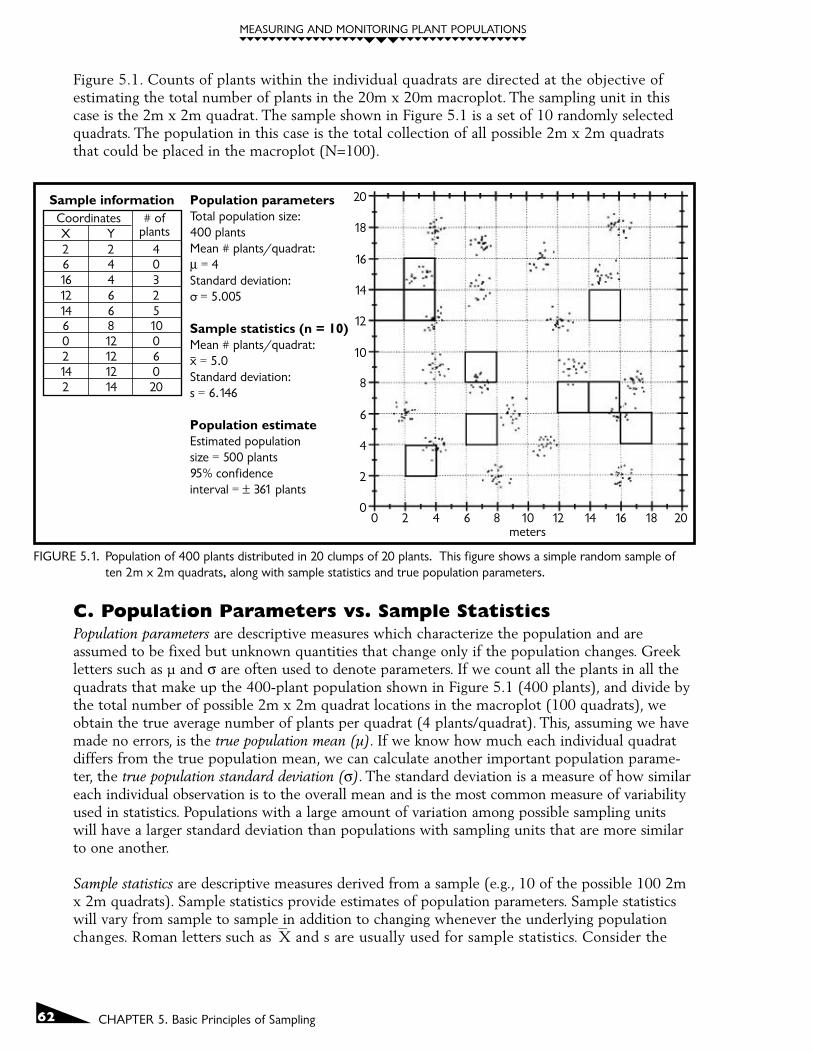
MEASURING AND MONITORING PLANT POPULATIONS
62 CHAPTER 5. Basic Principles of Sampling
Figure 5.1. Counts of plants within the individual quadrats are directed at the objective ofestimating the total number of plants in the 20m x 20m macroplot. The sampling unit in thiscase is the 2m x 2m quadrat. The sample shown in Figure 5.1 is a set of 10 randomly selectedquadrats. The population in this case is the total collection of all possible 2m x 2m quadratsthat could be placed in the macroplot (N=100).
C. Population Parameters vs. Sample StatisticsPopulation parameters are descriptive measures which characterize the population and areassumed to be fixed but unknown quantities that change only if the population changes. Greekletters such as µ and σ are often used to denote parameters. If we count all the plants in all thequadrats that make up the 400-plant population shown in Figure 5.1 (400 plants), and divide bythe total number of possible 2m x 2m quadrat locations in the macroplot (100 quadrats), weobtain the true average number of plants per quadrat (4 plants/quadrat). This, assuming we havemade no errors, is the true population mean (µ). If we know how much each individual quadratdiffers from the true population mean, we can calculate another important population parame-ter, the true population standard deviation (σ). The standard deviation is a measure of how similareach individual observation is to the overall mean and is the most common measure of variabilityused in statistics. Populations with a large amount of variation among possible sampling unitswill have a larger standard deviation than populations with sampling units that are more similarto one another.
Sample statistics are descriptive measures derived from a sample (e.g., 10 of the possible 100 2mx 2m quadrats). Sample statistics provide estimates of population parameters. Sample statisticswill vary from sample to sample in addition to changing whenever the underlying populationchanges. Roman letters such asX and s are usually used for sample statistics. Consider the
00
2
4
6
8
10
12
14
16
18
20Population parametersTotal population size:400 plantsMean # plants/quadrat:µ = 4Standard deviation:o = 5.005
Sample statistics (n = 10)Mean # plants/quadrat:x = 5.0Standard deviation:s = 6.146
Population estimateEstimated populationsize = 500 plants95% confidenceinterval = ± 361 plants
Sample informationCoordinatesX Y2 2 46 4 016 4 312 6 214 6 56 8 100 12 02 12 614 12 02 14 20
# ofplants
2 4 6 8 10meters
12 14 16 18 20
FIGURE 5.1. Population of 400 plants distributed in 20 clumps of 20 plants. This figure shows a simple random sample often 2m x 2m quadrats, along with sample statistics and true population parameters.

63
MEASURING AND MONITORING PLANT POPULATIONS
CHAPTER 5. Basic Principles of Sampling
following simple example where a sample of three sampling units yields values of 9, 10, and 14plants/quadrat:
The sample mean (X) = (9+10+14)/3 = 11 plants/quadrat
We could also calculate from this sample a sample standard deviation (s). The sample standarddeviation describes how similar each individual observation is to the sample mean. The derivationof a standard deviation (in case you want to calculate one by hand) is provided in Appendix 8.The standard deviation is easily calculated with a simple hand calculator using the "s" or "σn-1" key.
The standard deviation (s) for the simple example above is 2.65 plants/quadrat.
Consider another simple example with sampling unit values of 2, 10, and 21 plants/quadrat.
The mean (X) = (2+10+21)/3 = 11 plants/quadrat
The standard deviation (s) for this example is 9.54 plants/quadrat.
Thus, both examples have a sample mean of 11 plants/quadrat, but the second one has a higherstandard deviation (9.54 plants/quadrat) than the first (2.65 plants/quadrat), because theindividual quadrat values differ more from one another in the second example.
In the example shown in Figure 5.1, the true population mean is 4.00 plants/quadrat, whereasthe sample mean is 5.00 plants/quadrat. The true population standard deviation is 5.005plants/quadrat, whereas the sample standard deviation is 6.146 plants/quadrat.
D. Accuracy vs. PrecisionAccuracy is the closeness of a measured or computed value to its true value. Precision is thecloseness of repeated measurements of the same quantity. A simple example will help illustratethe difference between these two terms. Two quartz clocks, equally capable of tracking time, aresitting side-by-side on a table. Someone comes by and advances one of the clocks by 1 hour.Both clocks will be equally "precise" at tracking time, but one of them will not be "accurate."
Efficient sampling designs try to achieve high precision. When we sample to estimate some popula-tion parameter, our sample standard deviation gives us a measure of the repeatability, or preci-sion of our sample; it does not allow us to assess the accuracy of our sample. If counts of plantswithin different quadrats of a sample are similar to one another (e.g., the example above with amean of 11 and a standard deviation = 2.65) then it is likely that different independent samplesfrom the same population will yield similar sample means and give us high precision. Whenquadrat counts within a sample are highly variable (e.g., the example above with a mean of 11and a standard deviation of 9.54), individual sample means from separate independent samplesmay be very different from one another giving us low precision. In either case, if the countingprocess is biased (perhaps certain color morphs or growth forms of individuals are overlooked),results may be inaccurate.
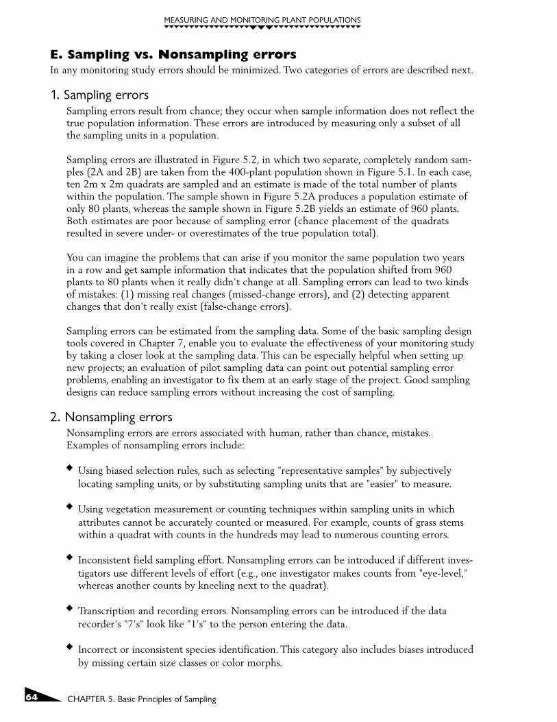
MEASURING AND MONITORING PLANT POPULATIONS
64 CHAPTER 5. Basic Principles of Sampling
E. Sampling vs. Nonsampling errorsIn any monitoring study errors should be minimized. Two categories of errors are described next.
1. Sampling errorsSampling errors result from chance; they occur when sample information does not reflect thetrue population information. These errors are introduced by measuring only a subset of allthe sampling units in a population.
Sampling errors are illustrated in Figure 5.2, in which two separate, completely random sam-ples (2A and 2B) are taken from the 400-plant population shown in Figure 5.1. In each case,ten 2m x 2m quadrats are sampled and an estimate is made of the total number of plantswithin the population. The sample shown in Figure 5.2A produces a population estimate ofonly 80 plants, whereas the sample shown in Figure 5.2B yields an estimate of 960 plants.Both estimates are poor because of sampling error (chance placement of the quadratsresulted in severe under- or overestimates of the true population total).
You can imagine the problems that can arise if you monitor the same population two yearsin a row and get sample information that indicates that the population shifted from 960plants to 80 plants when it really didn't change at all. Sampling errors can lead to two kindsof mistakes: (1) missing real changes (missed-change errors), and (2) detecting apparentchanges that don't really exist (false-change errors).
Sampling errors can be estimated from the sampling data. Some of the basic sampling designtools covered in Chapter 7, enable you to evaluate the effectiveness of your monitoring studyby taking a closer look at the sampling data. This can be especially helpful when setting upnew projects; an evaluation of pilot sampling data can point out potential sampling errorproblems, enabling an investigator to fix them at an early stage of the project. Good samplingdesigns can reduce sampling errors without increasing the cost of sampling.
2. Nonsampling errorsNonsampling errors are errors associated with human, rather than chance, mistakes.Examples of nonsampling errors include:
� Using biased selection rules, such as selecting "representative samples" by subjectivelylocating sampling units, or by substituting sampling units that are "easier" to measure.
� Using vegetation measurement or counting techniques within sampling units in whichattributes cannot be accurately counted or measured. For example, counts of grass stemswithin a quadrat with counts in the hundreds may lead to numerous counting errors.
� Inconsistent field sampling effort. Nonsampling errors can be introduced if different inves-tigators use different levels of effort (e.g., one investigator makes counts from "eye-level,"whereas another counts by kneeling next to the quadrat).
� Transcription and recording errors. Nonsampling errors can be introduced if the datarecorder's "7's" look like "1's" to the person entering the data.
� Incorrect or inconsistent species identification. This category also includes biases introducedby missing certain size classes or color morphs.

65
MEASURING AND MONITORING PLANT POPULATIONS
CHAPTER 5. Basic Principles of Sampling
Because sampling designs are based on the assumption that nonsampling errors are zero, the num-ber of nonsampling errors needs to be minimized. Ensure that your sampling unit makes sense forthe type of vegetation measurement technique you have selected. When different personnel areused in the same monitoring study, conduct rigorous training and testing to ensure consistency incounts or measurements. Design field data forms (Chapter 9) that are easy to use and easy fordata transcribers to interpret. Proof all data entered into computer programs to ensure that enterednumbers are correct. In contrast to sampling errors, the probability of nonsampling errors occur-ring cannot be assessed from pilot sample data.
00
2
4
6
8
10
12
14
16
18
20Population parametersTotal population size:400 plantsMean # plants/quadrat:µ = 4Standard deviation:o = 5.005
Sample statistics (n = 10)Mean # plants/quadrat:x = 0.8Standard deviation:s = 1.75
Population estimateEstimated populationsize = 80 plants95% confidenceinterval = ± 119 plants
Sample informationCoordinatesX Y16 2 516 4 318 4 00 10 06 10 014 12 04 14 08 16 012 16 012 18 0
# ofplants
2 4 6 8 10meters
12 14 16 18 20
FIGURE 5.2. Examples of sampling errors from sampling the 400-plant population. The population estimates of 80 plantsand 960 plants are far from the true population of 400 plants.
00
2
4
6
8
10
12
14
16
18
20Population parametersTotal population size:400 plantsMean # plants/quadrat:µ = 4Standard deviation:o = 5.005
Sample statistics (n = 10)Mean # plants/quadrat:x = 9.6Standard deviation:s = 5.58
Population estimateEstimated populationsize = 960 plants95% confidenceinterval = ± 379 plants
Sample information
A
BCoordinatesX Y16 0 510 2 1116 4 314 6 512 8 186 8 104 16 92 12 610 16 914 14 20
# ofplants
2 4 6 8 10meters
12 14 16 18 20
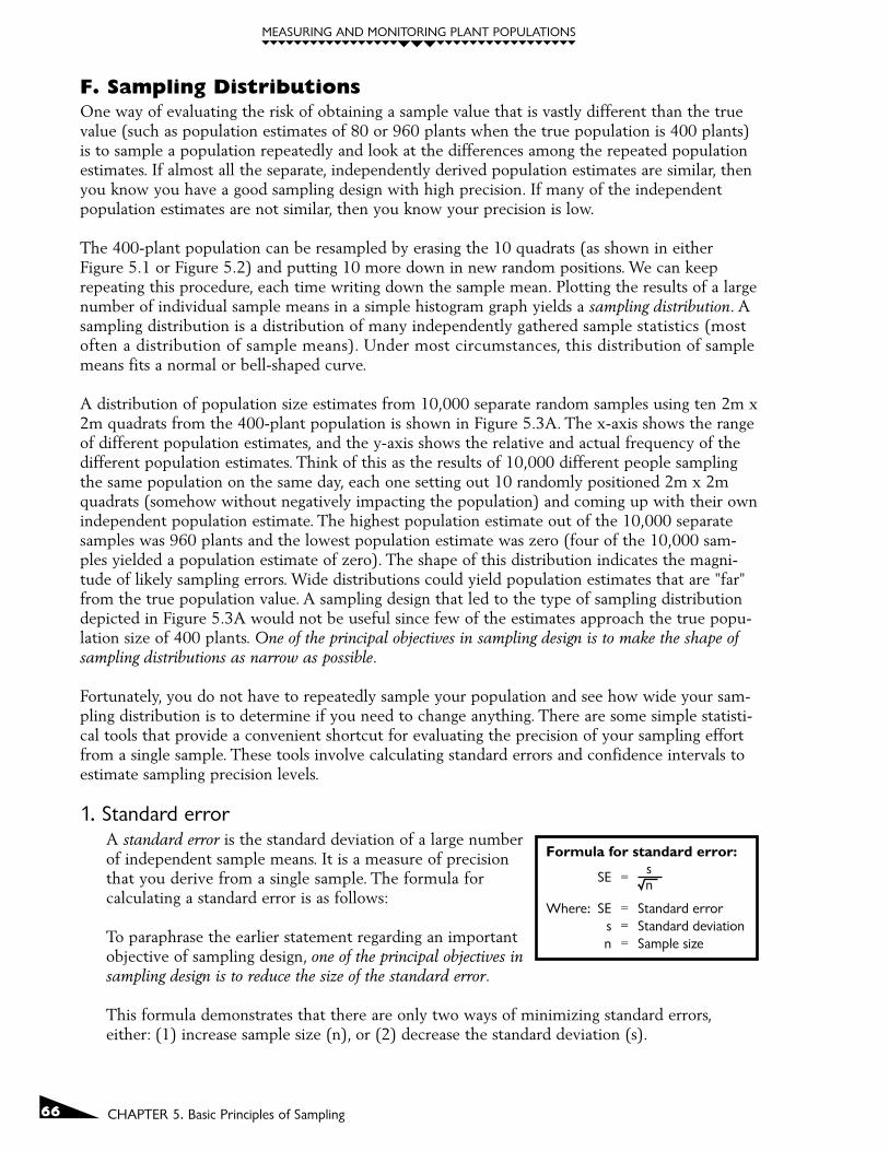
MEASURING AND MONITORING PLANT POPULATIONS
66 CHAPTER 5. Basic Principles of Sampling
F. Sampling DistributionsOne way of evaluating the risk of obtaining a sample value that is vastly different than the truevalue (such as population estimates of 80 or 960 plants when the true population is 400 plants)is to sample a population repeatedly and look at the differences among the repeated populationestimates. If almost all the separate, independently derived population estimates are similar, thenyou know you have a good sampling design with high precision. If many of the independentpopulation estimates are not similar, then you know your precision is low.
The 400-plant population can be resampled by erasing the 10 quadrats (as shown in eitherFigure 5.1 or Figure 5.2) and putting 10 more down in new random positions. We can keeprepeating this procedure, each time writing down the sample mean. Plotting the results of a largenumber of individual sample means in a simple histogram graph yields a sampling distribution. Asampling distribution is a distribution of many independently gathered sample statistics (mostoften a distribution of sample means). Under most circumstances, this distribution of samplemeans fits a normal or bell-shaped curve.
A distribution of population size estimates from 10,000 separate random samples using ten 2m x2m quadrats from the 400-plant population is shown in Figure 5.3A. The x-axis shows the rangeof different population estimates, and the y-axis shows the relative and actual frequency of thedifferent population estimates. Think of this as the results of 10,000 different people samplingthe same population on the same day, each one setting out 10 randomly positioned 2m x 2mquadrats (somehow without negatively impacting the population) and coming up with their ownindependent population estimate. The highest population estimate out of the 10,000 separatesamples was 960 plants and the lowest population estimate was zero (four of the 10,000 sam-ples yielded a population estimate of zero). The shape of this distribution indicates the magni-tude of likely sampling errors. Wide distributions could yield population estimates that are "far"from the true population value. A sampling design that led to the type of sampling distributiondepicted in Figure 5.3A would not be useful since few of the estimates approach the true popu-lation size of 400 plants. One of the principal objectives in sampling design is to make the shape ofsampling distributions as narrow as possible.
Fortunately, you do not have to repeatedly sample your population and see how wide your sam-pling distribution is to determine if you need to change anything. There are some simple statisti-cal tools that provide a convenient shortcut for evaluating the precision of your sampling effortfrom a single sample. These tools involve calculating standard errors and confidence intervals toestimate sampling precision levels.
1. Standard errorA standard error is the standard deviation of a large numberof independent sample means. It is a measure of precisionthat you derive from a single sample. The formula forcalculating a standard error is as follows:
To paraphrase the earlier statement regarding an importantobjective of sampling design, one of the principal objectives insampling design is to reduce the size of the standard error.
This formula demonstrates that there are only two ways of minimizing standard errors,either: (1) increase sample size (n), or (2) decrease the standard deviation (s).
Formula for standard error:
Where: SE = Standard errors = Standard deviationn = Sample size
SE =sn

67
MEASURING AND MONITORING PLANT POPULATIONS
CHAPTER 5. Basic Principles of Sampling
� Increase sample size. A new sampling distribution of 10,000 separate random samplesdrawn from our example population is shown in Figure 5.3B. This distribution came fromrandomly drawing samples of twenty 2m x 2m quadrats instead of the ten quadrats used tocreate the sampling distribution in Figure 5.3A. This increase in sample size from 10 to 20provides a 29.3% improvement in precision (as measured by the reduced size of thestandard error).
� Decrease sample standard deviation. Another sampling distribution of 10,000 separaterandom samples drawn from our 400-plant population is shown in Figure 5.3C. Thesampling design used to create this distribution of population estimates is similar to
0.10
0.08
0.12
0.06
0.04
0.02
prop
ortio
n pe
r ba
r
Cou
nt
0.0800 900
0.4m x 10m, n = 20
2m x 2m, n = 20
2m x 2m, n = 10
1000700600500estimated total population
40030020010000
200100
300
500
700
900
1100
400
600
800
1000
1200
0.05
0.04
0.06
0.07
0.08
0.03
0.02
0.01
prop
ortio
n pe
r ba
r
Cou
nt
0.0800 900 1000700600500
estimated total population4003002001000
0
200
100
300
500
700
400
600
800
0.05
0.04
0.06
0.03
0.02
0.01
prop
ortio
n pe
r ba
r
Cou
nt
0.0800 900 1000700600500
estimated total population4003002001000
0
200
100
300
500
400
600
A
B
C
FIGURE 5.3. Sampling distributions from three separate sampling designs used on the 400-plantpopulation. All distributions were created by sampling the population 10,000 separatetimes. The smooth lines show a normal bell-shaped curve fit to the data. Figure 3Ashows a sampling distribution where ten 2m x 2m quadrats were used. Figure 3Bshows a sampling distribution where twenty 2m x 2m quadrats were used. Figure 3Cshows a sampling distribution where twenty 0.4m x 10m quadrats were used.
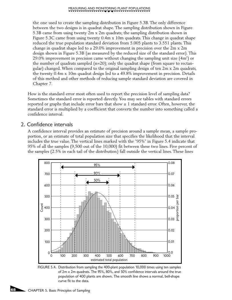
MEASURING AND MONITORING PLANT POPULATIONS
68 CHAPTER 5. Basic Principles of Sampling
the one used to create the sampling distribution in Figure 5.3B. The only differencebetween the two designs is in quadrat shape. The sampling distribution shown in Figure5.3B came from using twenty 2m x 2m quadrats; the sampling distribution shown inFigure 5.3C came from using twenty 0.4m x 10m quadrats. This change in quadrat shapereduced the true population standard deviation from 5.005 plants to 3.551 plants. Thischange in quadrat shape led to a 29.0% improvement in precision over the 2m x 2mdesign shown in Figure 5.3B (as measured by the reduced size of the standard error). This29.0% improvement in precision came without changing the sampling unit size (4m2) orthe number of quadrats sampled (n=20); only the quadrat shape (from square to rectan-gular) changed. When compared to the original sampling design of ten 2m x 2m quadrats,the twenty 0.4m x 10m quadrat design led to a 49.8% improvement in precision. Detailsof this method and other methods of reducing sample standard deviation are covered inChapter 7.
How is the standard error most often used to report the precision level of sampling data?Sometimes the standard error is reported directly. You may see tables with standard errorsreported or graphs that include error bars that show ± 1 standard error. Often, however, thestandard error is multiplied by a coefficient that converts the number into something called aconfidence interval.
2. Confidence intervalsA confidence interval provides an estimate of precision around a sample mean, a sample pro-portion, or an estimate of total population size that specifies the likelihood that the intervalincludes the true value. The vertical lines marked with the "95%" in Figure 5.4 indicate that95% of all the samples (9,500 out of the 10,000) fit between these two lines. Five percent ofthe samples (2.5% in each tail of the distribution) fall outside the vertical lines. These lines
0.05
0.04
0.06
0.07
0.08
0.03
0.02
0.01
prop
ortio
n pe
r ba
r
Cou
nt
0.0800 900 1000700600500
estimated total population400
50%
95%
30020010000
200
100
300
500
400
600
700
800
FIGURE 5.4. Distribution from sampling the 400-plant population 10,000 times using ten samplesof 2m x 2m quadrats. The 95%, 80%, and 50% confidence intervals around the truepopulation of 400 plants are shown. The smooth line shows a normal, bell-shapecurve fit to the data.
80%
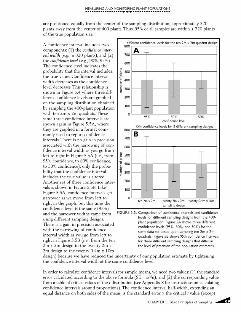
69
MEASURING AND MONITORING PLANT POPULATIONS
CHAPTER 5. Basic Principles of Sampling
are positioned equally from the center of the sampling distribution, approximately 320plants away from the center of 400 plants. Thus, 95% of all samples are within ± 320 plantsof the true population size.
A confidence interval includes twocomponents: (1) the confidence inter-val width (e.g., ± 320 plants); and (2)the confidence level (e.g., 90%, 95%).The confidence level indicates theprobability that the interval includesthe true value. Confidence intervalwidth decreases as the confidencelevel decreases. This relationship isshown in Figure 5.4 where three dif-ferent confidence levels are graphedon the sampling distribution obtainedby sampling the 400-plant populationwith ten 2m x 2m quadrats. Thesesame three confidence intervals areshown again in Figure 5.5A, wherethey are graphed in a format com-monly used to report confidenceintervals. There is no gain in precisionassociated with the narrowing of con-fidence interval width as you go fromleft to right in Figure 5.5A (i.e., from95% confidence, to 80% confidence,to 50% confidence); only the proba-bility that the confidence intervalincludes the true value is altered.Another set of three confidence inter-vals is shown in Figure 5.5B. LikeFigure 5.5A, confidence intervals getnarrower as we move from left toright in the graph, but this time theconfidence level is the same (95%)and the narrower widths came fromusing different sampling designs.There is a gain in precision associatedwith the narrowing of confidenceinterval width as you go from left toright in Figure 5.5B (i.e., from the ten2m x 2m design to the twenty 2m x2m design to the twenty 0.4m x 10mdesign) because we have reduced the uncertainty of our population estimate by tighteningthe confidence interval width at the same confidence level.
In order to calculate confidence intervals for sample means, we need two values: (1) the standarderror calculated according to the above formula (SE = s/√n), and (2) the corresponding valuefrom a table of critical values of the t distribution (see Appendix 8 for instructions on calculatingconfidence intervals around proportions). The confidence interval half-width, extending anequal distance on both sides of the mean, is the standard error × the critical t value (except
B
num
ber
of p
lant
s
twenty 2m x 2msampling design
95% confidence levels for 3 different sampling designs
0
200
100
300
500
400
600
700
800
ten 2m x 2m twenty 0.4m x 10m
A
num
ber
of p
lant
s80%
confidence level
different confidence levels for the ten 2m x 2m quadrat design
0
200
100
300
500
400
600
700
800
95% 50%
FIGURE 5.5. Comparison of confidence intervals and confidencelevels for different sampling designs from the 400-plant population. Figure 5A shows three differentconfidence levels (95%, 80%, and 50%) for thesame data set based upon sampling ten 2m x 2mquadrats. Figure 5B shows 95% confidence intervalsfor three different sampling designs that differ inthe level of precision of the population estimates.

MEASURING AND MONITORING PLANT POPULATIONS
70 CHAPTER 5. Basic Principles of Sampling
when sampling from finite populations, see below). The appropriate critical value of tdepends on the level of confidence desired and the number of sampling units (n) in the sam-ple. A table of critical values for the t distribution (Zar 1996) is found in Appendix 5. To usethis table, you must first select the appropriate confidence level column. If you want to be95% confident that your confidence interval includes the true mean, use the column headedα(2) = 0.05. For 90% confidence, use the column headed α(2) = 0.10. You use α(2) becauseyou are interested in a confidence interval on both sides of the mean. You then use the rowindicating the number of degrees of freedom (v), which is the number of sampling unitsminus one (n-1).
For example, if we sample 20 quadrats and come up with a mean of 4.0 plants and a stan-dard deviation of 5.005, here are the steps for calculating a 95% confidence interval aroundour sample mean:
The standard error (SE = s/√n) = 5.005/4.472 = 1.119.
The appropriate t value from Appendix 5 for 19 degrees of freedom (v) is 2.093.
One-half of our confidence interval width is then SE × t-value = 1.119 × 2.093 = 2.342.
Our 95% confidence interval can then be reported as 4.0 ± 2.34 plants/quadrat or we canreport the entire confidence interval width from 1.66 to 6.34 plants/quadrat. This indicates a95% chance that our interval from 1.66 plants/quadrat to 6.34 plants/quadrat includes thetrue value.
Another way to think of 95% confidence intervals calculated from sampling data is that theinterval specifies a range that should include the true value 95% of the time. If you are calculat-ing 95% confidence intervals and independently randomly sample a population 100 differenttimes, you should see that approximately 95 of the intervals will include the true mean and 5will miss it. This relationship is shown in Figure 5.6 where 100 independent population estimatesare graphed with 95% confidence intervals from the 400-plant populations using samples oftwenty 0.4m x 10m quadrats. You will notice that the solid dots, used to show each of the 100population estimates, fluctuate around the true population value of 400 plants. You will alsonotice that 96 out of 100 confidence intervals shown in Figure 5.6 include the true value. Ifthe confidence level had been set at 80%, then approximately 20 of the intervals would havefailed to include the true value. A 99% confidence level would have led to approximatelyonly one interval out of the 100 that did not include the true population size (in order tocapture the true value more often, the individual confidence interval widths for a 99%confidence level are wider than the confidence interval widths for a 95% confidence level).
G. Finite vs. Infinite PopulationsIf we are sampling with quadrats, there is a finite number of quadrats that can be placed in thearea to be sampled, assuming that no two quadrats overlap (this is called sampling withoutreplacement). If the sampled area is large, then the number of quadrats placed in the area maybe very large as well, but nonetheless finite. On the other hand, an infinite number of points orlines could be placed in the area to be sampled. This is because points, at least theoretically, aredimensionless, and lines are dimensionless in one direction. This means, at least for all practicalpurposes, that a population of points or of lines is infinite.
= 5.005 20

71
MEASURING AND MONITORING PLANT POPULATIONS
CHAPTER 5. Basic Principles of Sampling
If the area to be sampled is large relative to the area that is actually sampled, the distinction betweenfinite and infinite is of only theoretical interest. When, however, the area sampled makes up a signifi-cant portion of the area to be sampled, wecan apply the finite population correction factor,which reduces the size of the standard error.The most commonly used finite populationcorrection factor is shown to the right:
When n is small relative to N, the equationis close to 1, whereas when n is large relative to N, the value approaches zero. The standard error(s/√n) is multiplied by the finite population correction factor to yield a corrected standard errorfor the finite population.
Consider the following example. The density of plant species X is estimated within a 20m x 50mmacroplot (total area = 1000m2). This estimate is obtained by collecting data from randomlyselected 1m x 10m quadrats (10m2). Sampling without replacement, there are 100 possiblequadrat positions.
Thus, our population, N, is 100. Let’s say we take a random sample, n, of 30 of these quadrats andcalculate a mean of eight plants per quadrat and a standard deviation of four plants per quadrat.Our standard error is thus: s/√n = 4/√30 = 0.73. Although our sample mean is an unbiased estimatorof the true population mean and needs no correction, the standard error should be corrected by thefinite population correction factor shown on the top of page 72:
popu
latio
n es
timat
e
50 60 70 80independent samples
0
200
100
300
500
400
600
700
800
0 10 20 30 40 90 100
FIGURE 5.6. Population estimates from 100 separate random samples from the 400-plant population.Each sample represents the population estimate from sampling twenty 0.4m x 10mquadrats. The horizontal line through the graph indicates the true population of 400plants. Vertical bars represent 95% confidence intervals. Four of the intervals miss thetrue population size.
Formula for the finite population correction:
Where: N = total number of potential quadrat positionsn = number of quadrats sampled
FPC = N - nN
total area 1000m2
quadrat area 10m2=

MEASURING AND MONITORING PLANT POPULATIONS
72 CHAPTER 5. Basic Principles of Sampling
Since the standard error is one ofthe factors used to calculate con-fidence intervals (the other is theappropriate value of t from a ttable), correcting the standarderror with the finite populationcorrection factor makes theresulting confidence interval
narrower. It does this, however, only if n is sufficiently large relative to N. A rule of thumb is thatunless the ratio n/N is greater than .05 (i.e., you are sampling more than 5% of the populationarea), there is little to be gained by applying the finite population correction factor to yourstandard error.
The finite population correction factor is also important in sample size determination (Chapter 7)and in adjusting test statistics (Chapter 11). The finite population correction factor works, how-ever, only with finite populations, which we will have when using quadrats, but will not havewhen using points or lines.
H. False-Change Errors and Statistical Power ConsiderationsThese terms relate to situations where two or more sample means or proportions are being com-pared with some statistical test. This comparison may be between two or more places or thesame place between two or more time periods. These terms are pertinent to both planning andinterpretation stages of a monitoringstudy. Consider a simple examplewhere you have sampled a popula-tion in two different years and nowyou want to determine whether achange took place between the twoyears. You usually start with theassumption, called the null hypothe-sis, that no change has taken place.There are two types of decisions thatyou can make when interpreting theresults of a monitoring study: (1) youcan decide that a change took place,or (2) you can decide that no changetook place. In either case, you caneither be right, or you can be wrong (Figure 5.7).
1. The change decision and false-change errors The conclusion that a change took place may lead to some kind of action. For example, if apopulation of a rare plant is thought to have declined, a change in management may beneeded. If a change did not actually occur, this constitutes a false-change error, a sort of falsealarm. Controlling this type of error is important because taking action unnecessarily can beexpensive (e.g., a range permittee is not going to want to change the grazing intensity if adecline in a rare plant population really didn't take place). There will be a certain probabilityof concluding that a change took place even if no difference actually occurred. The probabilityof this occurring is usually labeled the P-value, and it is one of the types of information thatcomes out of a statistical analysis of the data. The P-value reports the likelihood that the
no change hastaken place
monitoring for change — possible errors
there has beena real change
false-change error(Type I)
monitoringsystem detects a
change
no error(Power) 1 -
no error(1 - )
monitoringsystem detects no
change
missed-change error(Type II)
FIGURE 5.7. Four possible outcomes for a statistical test of some nullhypothesis, depending on the true state of nature.
Example of applying the finite population correction factor:
Where: SE' = corrected standard errorSE = uncorrected standard errorN = total number of potential quadrat positionsn = number of quadrats sampled
SE' = (SE) N - nN
SE' = (0.73) = 0.61100 - 30100

73
MEASURING AND MONITORING PLANT POPULATIONS
CHAPTER 5. Basic Principles of Sampling
observed difference was due to chance alone. For example, if a statistical test comparing twosample means yields a P-value of 0.24 this indicates that there is a 24% chance of obtainingthe observed result even if there is no true difference between the two sample means.
Some threshold value for this false-change error rate should be set in advance so that theP-value from a statistical test can be evaluated relative to the threshold. P-values from astatistical test that are smaller than or equal to the threshold are considered statistically"significant," whereas P-values that are larger than the threshold are considered statistically"nonsignificant." Statistically significant differences may or may not be ecologically significantdepending upon the magnitude of difference between the two values. The most commonlycited threshold for false-change errors is the 0.05 level; however, there is no reason to arbi-trarily adopt the 0.05 level as the appropriate threshold. The decision of what false-changeerror threshold to set depends upon the relative costs of making this type of mistake and theimpact of this error level on the other type of mistake, a missed-change error (see below).
2. The no-change decision, missed-change errors, and statistical powerThe conclusion that no change took place usually does not lead to changes in managementpractices. Failing to detect a true change constitutes a missed-change error. Controlling thistype of error is important because failing to take action when a true change actually occurredmay lead to the serious decline of a rare plant population.
Statistical power is the complement of the missed-change error rate (e.g., a missed-changeerror rate of 0.25 gives you a power of 0.75; a missed-change error rate of 0.05 gives you apower of 0.95). High power (a value close to 1), is desirable and corresponds to a low risk ofa missed-change error. Low power (a value close to 0) is not desirable because it correspondsto a high risk of a missed-change error.
Since power levels are directly related to missed-change error levels, either level can bereported and the other level can be easily calculated. Power levels are often reported insteadof missed-change error levels, because it seems easier to convey this concept in terms of thecertainty of detecting real changes. For example, the statement "I want to be at least 90%certain of detecting a real change of five plants/quadrat" (power is 0.90) is simpler to under-stand than the statement "I want the probability of missing a real change of five plants/quadratto be 10% or less" (missed-change error rate is 0.10).
An assessment of statistical power or missed-change errors has been virtually ignored in thefield of environmental monitoring. A survey of over 400 papers in fisheries and aquatic sci-ences found that 98% of the articles that reported nonsignificant results failed to report anypower results (Peterman 1990). A separate survey, reviewing toxicology literature, found highpower in only 19 out of 668 reports that failed to reject the null hypothesis (Hayes 1987).Similar surveys in other fields such as psychology or education have turned up "depressinglylow" levels of power (Brewer 1972; Cohen 1988).
3. Minimum detectable changeAnother sampling design concept that is directly related to statistical power and false-changeerror rates is the size of the change that you want to be able to detect. This will be referredto as the minimum detectable change or MDC. The MDC greatly influences power levels. Aparticular sampling design will be more likely to detect a true large change (i.e., with highpower) than to detect a true small change (i.e., with low power).

MEASURING AND MONITORING PLANT POPULATIONS
74 CHAPTER 5. Basic Principles of Sampling
Setting the MDC requires the consideration of ecological information for the species beingmonitored. How large of a change should be considered biologically meaningful? With alarge enough sample size, statistically significant changes can be detected for changes thathave no biological significance. For example, if an intensive monitoring design leads to theconclusion that the mean density of a plant population increased from 10.0 plants/m2 to10.1 plants/m2, does this represent some biologically meaningful change in populationdensity? Probably not.
Setting a reasonable MDC can be difficult when little is known about the natural history of aparticular plant species. Should a 30% change in the mean density of a rare plant populationbe cause for alarm? What about a 20% change or a 10% change? The MDC considerationsare likely to vary when assessing vegetation attributes other than density, such as cover orfrequency (Chapter 8). The initial MDC, set during the design of a new monitoring study,can be modified once monitoring information demonstrates the size and rate of populationfluctuations.
4. How to achieve high statistical powerStatistical power is related to four separate sampling design components by the followingfunction equation:
Power = a function of (s, n, MDC, and α)
where: s = standard deviationn = number of sampling units
MDC = minimum detectable change α = false-change error rate
Power can be increased in the following four ways:
1. Reducing standard deviation. This means altering the sampling design to reduce theamount of variation among sampling units (see Chapter 7).
2. Increasing the number of sampling units sampled. This method of increasing power isstraightforward, but keep in mind that increasing n has less of an effect than decreasing ssince the square root of sample size is used in the standard error equation (SE = s/√n).
3. Increasing the acceptable level of false-change errors (α).
4. Increasing the MDC.
Note that the first two ways of increasing power are related to making changes in thesampling design, whereas the other two ways are related to making changes in the samplingobjective (see Chapter 6).
5. Graphical comparisonsAs stated, power is driven by four different factors: standard deviation, sample size, mini-mum detectable change size, and false-change error rate. In this section we take a graphicallook at how altering these factors changes power. The comparisons in this section are basedupon sampling a fictitious plant population where we are interested in assessing plant densityrelative to an established threshold value of 25 plants/m2. Any true population densities less

75
MEASURING AND MONITORING PLANT POPULATIONS
CHAPTER 5. Basic Principles of Sampling
than 25 plants/m2 will trigger management action. We are only concerned with the questionof whether the density is lower than 25 plants/m2 and not whether the density is higher. Inthis example, our null hypothesis (HO) is that the population density equals 25 plants/m2 andour alternative hypothesis is that density is less than 25 plants/m2. The density value of 25plants/m2 is the most critical single density value since it defines the lower limit of acceptableplant density.
The figures in this section are all based upon sampling distributions where we happen toknow the true plant density. Recall that a sampling distribution is a bell-shaped curve thatdepicts the distribution of a large number of independently gathered sample statistics. Asampling distribution defines the range and relative probability of any possible sample mean.You are more likely to obtain sample means near the middle of the distribution than you areto obtain sample means near either tail of the distribution.
A sampling distribution based on sampling our fictitious population with a true mean densi-ty of 25 plants/m2 is shown in Figure 5.8A. This distribution is based on a sampling designusing thirty 1m x 1m quadrats where the true standard deviation is ± 20 plants/quadrat. If1,000 different people randomly sample and calculate a sample mean based upon their 30quadrat values, approximately half the individually drawn sample means will be less than 25plants/m2 and half will be greater than 25 plants/m2. Approximately 40% of the samples willyield sample means less than or equal to 24 plants/m2. A few of our 1,000 individuals willobtain estimates of the mean density that deviate from the true value by a large margin. Oneof the individuals will likely stand up and say, "my estimate of the mean density is 13plants/m2", even though the true density is actually 25 plants/m2. As interpreters of themonitoring information, we would conclude that since 999 of the 1,000 people obtainedestimates of the density that were greater than 13, the true density is probably not 13. Ourbest estimate of the true mean density will be the average of the 1,000 separate estimates(this average is likely to be extremely close to the actual true value).
Now that we have the benefit of 1,000 independent estimates of the true mean density, wecan return to the population at a later time, take a single random sample of thirty 1m x 1mquadrats, calculate the sample mean, and then ask the question, "what is the probability ofobtaining our sample mean value if the true population is still 25 plants/m2?" If our samplemean density turns out to be 24 plants/m2, would this lead to the conclusion that the popu-lation has crossed our threshold value? Seeing that our sample mean is lower than our targetvalue might raise some concerns, but we have no objective basis to conclude that the truepopulation is not, in fact, still actually 25 plants/m2. We learned in the previous paragraphthat a full 40% of possible samples are likely to yield mean densities of 24 plants/m2 or less ifthe true mean is 25 plants/m2. Thus, the probability of obtaining a single sample mean of 24plants/m2 or less when the true density is actually 25 plants/m2 is approximately 0.40.Obtaining a sample mean of 24 plants/m2 is consistent with the hypothesis that the truepopulation density is actually 25 plants/m2.
How small a sample mean do we need to obtain to feel confident that the population hasindeed dropped below 25 plants/m2? What will our interpretation be if we obtained a sam-ple mean of 22 plants/m2? Based upon our sampling distribution from the 1,000 people, theprobability of obtaining an estimate of 22 plants/m2 or less is around 20%, which representsa 1-in-5 chance that the true mean is still actually 25 plants/m2. Based upon the samplingdistribution from our 1,000 separate samplers, we can look at the likelihood of obtainingother different sample means. The probability of obtaining a sample of 20 plants/m2 is 8.5%,

MEASURING AND MONITORING PLANT POPULATIONS
76 CHAPTER 5. Basic Principles of Sampling
and the probability of obtaining a sample of 18 plants/m2 is 2.9% if the true mean density is25 plants/m2.
Since in most circumstances we will only have the results from a single sample (and not thebenefit of 1,000 independently gathered sample means), another technique must be used todetermine whether the population density has dropped below 25 plants/m2. One method isto run a statistical test that compares our sample mean to our density threshold value (25
00
5 10 15 20 25
if H0 is true and the true mean = 25
rela
tive
freq
uenc
y
18.830 35 40
A
= 0.62
= 0.05
observed mean density (plants/m2)
00
5 10 15 20 25
rela
tive
freq
uenc
y
18.830 35 40
B
observed mean density (plants/m2)
power = 0.38
if H0 is false and the true mean = 20
reject H0 do not reject H0
FIGURE 5.8. Example of sampling distributions for mean plant density in samples of 30 permanentquadrats where the among-quadrat standard deviation is 20 plants/m2. Part A is thesampling distribution for the case in which the null hypothesis, H0, is true and the truepopulation mean density is 25 plants/m2. The shaded area in part A is the criticalregion for = 0.05 and the vertical dashed line is at the critical sample mean value, 18.8.Part B is the sampling distribution for the case in which the H0 is false and the true meanis 20 plants/m2. In both distributions, a sample mean to the left of the vertical dashedline would reject H0, and to the right of it, would not reject H0. Power and values inpart B, in which H0 is false and the true mean = 20, are the proportion of samplemeans that would occur in the region in which H0 was rejected or not rejected,respectively (adapted from Peterman 1990).
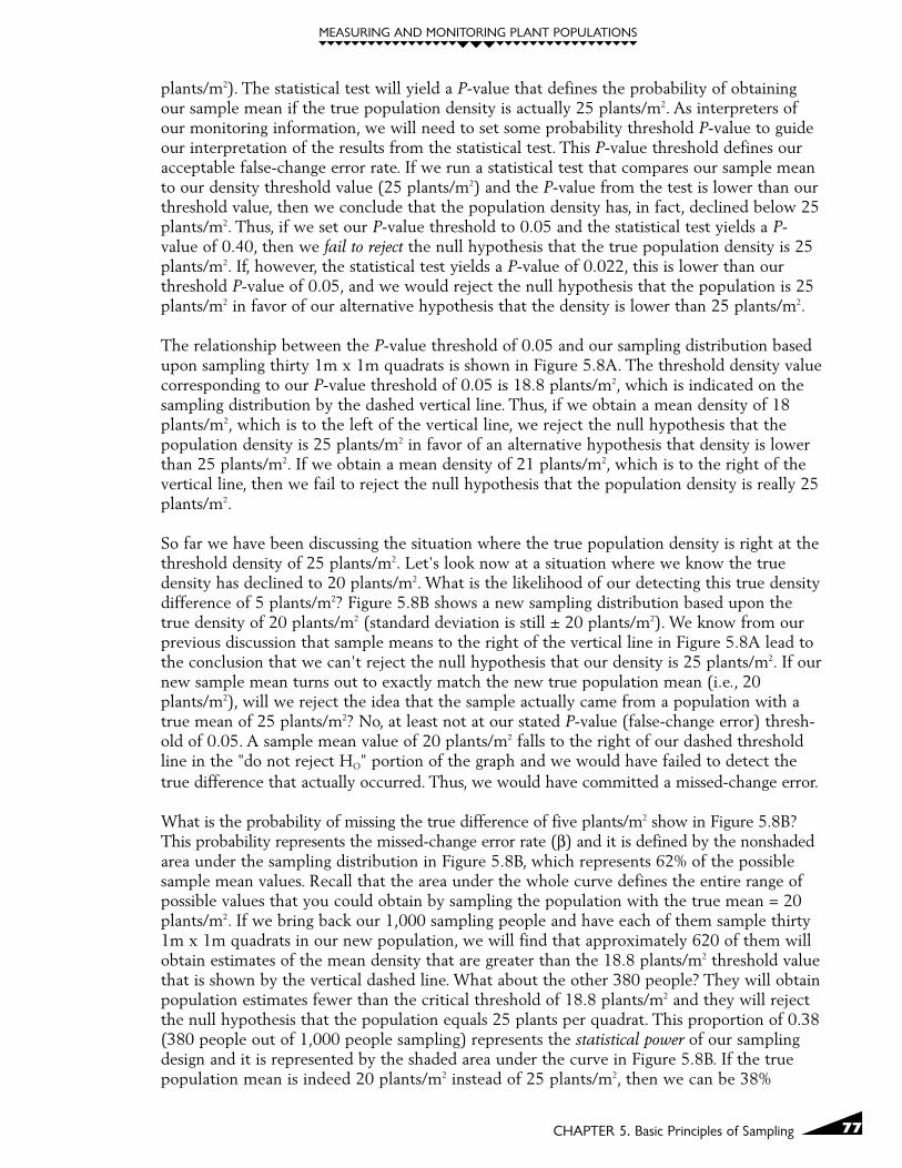
77
MEASURING AND MONITORING PLANT POPULATIONS
CHAPTER 5. Basic Principles of Sampling
plants/m2). The statistical test will yield a P-value that defines the probability of obtainingour sample mean if the true population density is actually 25 plants/m2. As interpreters ofour monitoring information, we will need to set some probability threshold P-value to guideour interpretation of the results from the statistical test. This P-value threshold defines ouracceptable false-change error rate. If we run a statistical test that compares our sample meanto our density threshold value (25 plants/m2) and the P-value from the test is lower than ourthreshold value, then we conclude that the population density has, in fact, declined below 25plants/m2. Thus, if we set our P-value threshold to 0.05 and the statistical test yields a P-value of 0.40, then we fail to reject the null hypothesis that the true population density is 25plants/m2. If, however, the statistical test yields a P-value of 0.022, this is lower than ourthreshold P-value of 0.05, and we would reject the null hypothesis that the population is 25plants/m2 in favor of our alternative hypothesis that the density is lower than 25 plants/m2.
The relationship between the P-value threshold of 0.05 and our sampling distribution basedupon sampling thirty 1m x 1m quadrats is shown in Figure 5.8A. The threshold density valuecorresponding to our P-value threshold of 0.05 is 18.8 plants/m2, which is indicated on thesampling distribution by the dashed vertical line. Thus, if we obtain a mean density of 18plants/m2, which is to the left of the vertical line, we reject the null hypothesis that thepopulation density is 25 plants/m2 in favor of an alternative hypothesis that density is lowerthan 25 plants/m2. If we obtain a mean density of 21 plants/m2, which is to the right of thevertical line, then we fail to reject the null hypothesis that the population density is really 25plants/m2.
So far we have been discussing the situation where the true population density is right at thethreshold density of 25 plants/m2. Let's look now at a situation where we know the truedensity has declined to 20 plants/m2. What is the likelihood of our detecting this true densitydifference of 5 plants/m2? Figure 5.8B shows a new sampling distribution based upon thetrue density of 20 plants/m2 (standard deviation is still ± 20 plants/m2). We know from ourprevious discussion that sample means to the right of the vertical line in Figure 5.8A lead tothe conclusion that we can't reject the null hypothesis that our density is 25 plants/m2. If ournew sample mean turns out to exactly match the new true population mean (i.e., 20plants/m2), will we reject the idea that the sample actually came from a population with atrue mean of 25 plants/m2? No, at least not at our stated P-value (false-change error) thresh-old of 0.05. A sample mean value of 20 plants/m2 falls to the right of our dashed thresholdline in the "do not reject HO" portion of the graph and we would have failed to detect thetrue difference that actually occurred. Thus, we would have committed a missed-change error.
What is the probability of missing the true difference of five plants/m2 show in Figure 5.8B?This probability represents the missed-change error rate (β) and it is defined by the nonshadedarea under the sampling distribution in Figure 5.8B, which represents 62% of the possiblesample mean values. Recall that the area under the whole curve defines the entire range ofpossible values that you could obtain by sampling the population with the true mean = 20plants/m2. If we bring back our 1,000 sampling people and have each of them sample thirty1m x 1m quadrats in our new population, we will find that approximately 620 of them willobtain estimates of the mean density that are greater than the 18.8 plants/m2 threshold valuethat is shown by the vertical dashed line. What about the other 380 people? They will obtainpopulation estimates fewer than the critical threshold of 18.8 plants/m2 and they will rejectthe null hypothesis that the population equals 25 plants per quadrat. This proportion of 0.38(380 people out of 1,000 people sampling) represents the statistical power of our samplingdesign and it is represented by the shaded area under the curve in Figure 5.8B. If the truepopulation mean is indeed 20 plants/m2 instead of 25 plants/m2, then we can be 38%

MEASURING AND MONITORING PLANT POPULATIONS
78 CHAPTER 5. Basic Principles of Sampling
(power = 0.38) sure that we will detect this true difference of five plants/m2. With this par-ticular sampling design (thirty 1m x 1m quadrats) and a false-change error rate of α=0.05,we run a 62% chance (β=0.62) that we will commit a missed-change error (i.e., fail to detectthe true difference of five plants/m2). If the difference of five plants/m2 is biologically impor-tant, a power of only 0.38 would not be satisfactory.
We can improve the low-power situation in four different ways: (1) increase the acceptablefalse-change error rate; (2) increase the acceptable MDC; (3) increase sample size; or (4)decrease the standard deviation. New paired sampling distributions illustrate the influence ofmaking each of these changes.
a. Increasing the acceptable false-change error rate
In Figure 5.8B, a false-change error rate of α=0.05 resulted in a missed-change error rate ofβ=0.62 to detect a difference of five plants/m2. Given these error rates, we are more than 12times more likely to commit a missed-change error than we are to commit a false-changeerror. What happens to our missed-change error rate if we specify a new, higher false-changeerror rate? Shifting our false-change error rate from α=0.05 to α=0.10 is illustrated in Figure 5.9
00
5 10 15 25
if H0 is true and the true mean = 25
rela
tive
freq
uenc
y
20.230 35 40
A
= 0.47
observed mean density (plants/m2)
= 0.10
00
5 10 15 20 25
rela
tive
freq
uenc
y
20.230 35 40
B
observed mean density (plants/m2)
power = 0.53
if H0 is false and the true mean = 20
FIGURE 5.9. The critical region for the false-change error in the sampling distributions from Figure5.8 has been increased from = 0.05 to = 0.10. Part B, in which the H0 is false andthe true mean = 20, shows that power is larger for = 0.10 than for Figure 5.8 where = 0.05 (adapted from Peterman 1990).

79
MEASURING AND MONITORING PLANT POPULATIONS
CHAPTER 5. Basic Principles of Sampling
for the same sampling distributions shown in Figure 5.8. Our critical density threshold at theP=0.10 level is now 20.21 plants/m2, and our missed-change error rate has dropped fromβ=0.62 down to β=0.47 (i.e., the power to detect a true five plant/m2 difference went from0.38 to 0.53). A sample mean of 20 plants/m2 will now lead to the correct conclusion that adifference of five plants/m2 between the populations does exist. Of course, the penalty wepay for increasing our false-change error rate is that we are now twice as likely to concludethat a difference exists in situations when there is no true difference and our populationmean is actually 25 plants/m2. Changing the false-change error rate even more, to α=0.20,(Figure 5.10) reduces the probability of making a missed-change error down to β=0.29 (i.e.,giving us a power of 0.71 to detect a true difference of five plants/m2).
b. Increasing the acceptable MDC
Any sampling design is more likely to detect a true large difference than a true small differ-ence. As the magnitude of the difference increases, we will see an increase in the power todetect the difference. This relationship is shown in Figure 5.11B, where we see a samplingdistribution with a true mean density of 15 plants/m2, which is 10 plants/m2 below ourthreshold density of 25 plants/m2. The false-change error rate is set at α=0.05 in this example.
00
5 10 15 20
if H0 is true and the true mean = 25
rela
tive
freq
uenc
y
21.9 30 35 40
FIGURE 5.10. The critical region for the false-change error in the sampling distributions fromFigure 5.8 has been increased from = 0.05 to = 0.20. Part B, in which theH0 is false and the true mean = 20, shows that power is larger for = 0.20 thanfor Figure 5.8 where = 0.05 or Figure 5.9 where = 0.10. Again, a samplemean to the left of the vertical dashed line would reject H0, while one to theright of it would not reject H0 (adapted from Peterman 1990).
A
00
5 10 15 20observed mean density (plants/m2)
rela
tive
freq
uenc
y
21.9 30 35 40
B
= 0.29power = 0.71
= 0.20
if H0 is false and the true mean = 20
observed mean density (plants/m2)

MEASURING AND MONITORING PLANT POPULATIONS
80 CHAPTER 5. Basic Principles of Sampling
This figure shows that the statistical power to detect this larger difference of 10 plants/m2
(25 plants/m2 to 15 plants/m2) is 0.85 compared with the original power value of 0.38 todetect the difference of five plants/m2 (25 plants/m2 to 20 plants/m2). Thus, with a false-change error rate of 0.05, we can be 85% certain of detecting a difference from our 25plants/m2 threshold of 10 plants/m2 or greater. If we raised our false-change error fromα=0.05 to α=0.10 (not shown in Figure 5.11), our power value would rise to 0.92, whichcreates a sampling situation where our two error rates are nearly equal (α=0.10, β=0.08).
c. Increasing the sample size
The sampling distributions shown in Figures 5.8 to 5.11 were all created by sampling thepopulations with n=30 1m x 1m quadrats. Any increase in sample size will lead to a subse-quent increase in power to detect some specified minimum detectable difference. Thisincrease in power results from the sampling distributions becoming narrower. Sampling dis-tributions based on samples of n=50 are shown in Figure 5.12 where the true differencebetween the two populations is once again five plants/m2 with a false-change error ratethreshold of α=0.05. The increase in sample size led to an increase in power from
00
5 10 15 20 25
if H0 is true and the true mean = 25
rela
tive
freq
uenc
y
18.8 30 35 40
FIGURE 5.11. Part A is the same as Figure 5.8; in part B, the true population mean is 15 plants/m2
instead of the 20 plants/m2 shown in Figure 5.8. Note that power increases(and decreases) when the new true population mean gets further from the originaltrue mean of 25 plants/m2. Again, a sample mean to the left of the vertical dashedline would reject H0, while one to the right of it would not reject H0 (adapted fromPeterman 1990).
A
00
5 10 15 20 25observed mean density (plants/m2)
rela
tive
freq
uenc
y
18.8 30 35 40
B
= 0.15power = 0.85
= 0.05
observed mean density (plants/m2)
if H0 is false and the true mean = 15
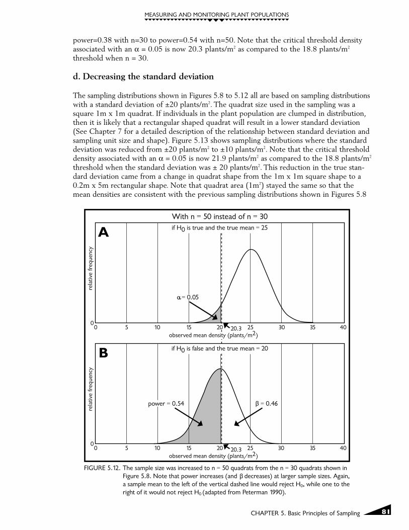
81
MEASURING AND MONITORING PLANT POPULATIONS
CHAPTER 5. Basic Principles of Sampling
power=0.38 with n=30 to power=0.54 with n=50. Note that the critical threshold densityassociated with an α = 0.05 is now 20.3 plants/m2 as compared to the 18.8 plants/m2
threshold when n = 30.
d. Decreasing the standard deviation
The sampling distributions shown in Figures 5.8 to 5.12 all are based on sampling distributionswith a standard deviation of ±20 plants/m2. The quadrat size used in the sampling was asquare 1m x 1m quadrat. If individuals in the plant population are clumped in distribution,then it is likely that a rectangular shaped quadrat will result in a lower standard deviation(See Chapter 7 for a detailed description of the relationship between standard deviation andsampling unit size and shape). Figure 5.13 shows sampling distributions where the standarddeviation was reduced from ±20 plants/m2 to ±10 plants/m2. Note that the critical thresholddensity associated with an α = 0.05 is now 21.9 plants/m2 as compared to the 18.8 plants/m2
threshold when the standard deviation was ± 20 plants/m2. This reduction in the true stan-dard deviation came from a change in quadrat shape from the 1m x 1m square shape to a0.2m x 5m rectangular shape. Note that quadrat area (1m2) stayed the same so that themean densities are consistent with the previous sampling distributions shown in Figures 5.8
00
5 10 15 25
if H0 is true and the true mean = 25
With n = 50 instead of n = 30
rela
tive
freq
uenc
y
30 35 40
FIGURE 5.12. The sample size was increased to n = 50 quadrats from the n = 30 quadrats shown inFigure 5.8. Note that power increases (and decreases) at larger sample sizes. Again,a sample mean to the left of the vertical dashed line would reject H0, while one to theright of it would not reject H0 (adapted from Peterman 1990).
A
00
5 10 15 20 25observed mean density (plants/m2)
rela
tive
freq
uenc
y
30 35 40
B
power = 0.54 = 0.46
= 0.05
observed mean density (plants/m2)
if H0 is false and the true mean = 20
20 20.3
20.3

MEASURING AND MONITORING PLANT POPULATIONS
82 CHAPTER 5. Basic Principles of Sampling
through 5.12. This reduction in standard deviation led to a dramatic improvement in power,from 0.38 (with sd = 20 plants/m2) to 0.85 (with sd = 10 plants/m2). Reducing the standarddeviation has a more direct impact on increasing power than increasing sample size, becausethe sample size is reduced by taking its square root in the standard error equation (SE = s/√n).Recall that the standard error provides an estimate of sampling precision from a single samplewithout having to enlist the support of 1,000 people who gather 1,000 independent samplemeans.
e. Power curves
The relationship between power and the different sampling design components that influencepower can also be displayed in power curve graphs. These graphs typically show power valueson the y-axis and either sample size, MDC, or standard deviation values on the x-axis. Figure5.14A shows statistical power graphed against different magnitudes of change for the samehypothetical data set described above and shown in Figures 5.8 to 5.11. Four different powercurve lines are shown, one for each of the following four different false-change (α) error rates:0.01, 0.05, 0.10, and 0.20. The power curves are based on sampling with a sample size of 30
00
5 10 15
if H0 is true and the true mean = 25
With s = 10 instead of s = 20
rela
tive
freq
uenc
y
30 35 40
FIGURE 5.13. The standard deviation (s) of 20 plants/m2 shown in Figure 5.8 is reduced to tenplants/m2. Note that power increases (and decreases), as the standard deviationdecreases. Again, a sample mean to the left of the vertical dashed line would rejectH0, while one to the right of it would not reject H0 (adapted from Peterman 1990).
A
00
5 10 15 20
observed mean density (plants/m2)
rela
tive
freq
uenc
y
30 35 40
B
power = 0.85 = 0.15
= 0.05
observed mean density (plants/m2)
if H0 is false and the true mean = 20
20 21.9
21.9

83
MEASURING AND MONITORING PLANT POPULATIONS
CHAPTER 5. Basic Principles of Sampling
quadrats and a standard deviation of 20 plants/m2. For any particular false-change error rate,power increases as the magnitude of the minimum detectable change increases. When α=0.05,the power to detect small changes is very low (Figure 5.14A). For example, we have only a13% chance of detecting a difference of 2 plants/m2 (i.e., a density of 23 plants/m2 which is 2plants/m2 below our threshold value of 25 plants/m2). In contrast, we can be 90% sure ofdetecting a minimum difference of 11 plants/m2. We can also attain higher power by increasing
0
0.1
0.2
0.3
0.4
0.5
0.6
0.7
0.8
0.9
1
2 3 4 5 6 7 8 9 10 11 12 13 14minimum detectable change size
pow
er
15 16 17 18 19 20
= 0.
20
= 0.
10
= 0.
05
= 0.
01
An = 30sd = 20
0
0.1
0.2
0.3
0.4
0.5
0.6
0.7
0.8
0.9
1
2 3 4 5 6 7 8 9 10 11 12 13 14minimum detectable change size
pow
er
15 16 17 18 19 20
= 0.
20=
0.10
= 0.
05
= 0.
01
Bn = 50sd = 20
FIGURE 5.14. Power curves showing power values for various magnitudes of minimum detectable changeand false-change error rates when the standard deviation is 20. Part A shows power curveswith a sample size of 30. Part B shows power curves with a sample size of 50.

MEASURING AND MONITORING PLANT POPULATIONS
84 CHAPTER 5. Basic Principles of Sampling
the false-change error rate. The power to detect a change of eight plants/m2 is only 0.41when α=0.01, but it increases to 0.69 at α=0.05, to 0.81 at α=0.10, and to 0.91 at α=0.20.
A different set of power curves are shown in Figure 5.14B where the sample size is n=50 insteadof the n=30 shown in Figure 5.14A. This larger smaller sample size shifts all of the power curvesto the left, making it more likely that smaller changes will be detected. For example, with a false-change error rate of α=0.10, the power to detect a seven plant/m2 difference is 0.88 with asample size of n=50 quadrats compared to the power of 0.73 with a sample size of n=30quadrats.
Power curves that show the effect of reducing the standard deviation are shown in Figure5.15. Figure 5.15A is the same as Figure 5.14A where the standard deviation is 20 plants/m2.Figure 5.15B shows the same power curves except they are based on a standard deviation of10 plants/m2. The smaller standard deviation shifts all of the power curves to the left andresults in much steeper slopes. The smaller standard deviation leads to substantially higherpower levels for any particular MDC value. For example, the power to detect a change offive plants/m2 with a false change error rate of α=0.10 is only 0.53 in Figure 5.15A ascompared to the power of 0.92 in Figure 5.15B.
6. Setting false-change and missed-change error ratesBoth false-change and missed-change error rates can be reduced by sampling design changesthat increase sample size or decrease sample standard deviations. Missed-change and false-change error rates are inversely related, which means that reducing one will increase theother (but not proportionately) if no other changes are made. The decision of which type oferror is more important should be based on the nature of the changes you are trying todetermine, and the consequences of making either kind of mistake.
Because false-change and missed-change error rates are inversely related to each other, andbecause these errors have different consequences to different interest groups, there are differ-ent opinions as to what the "acceptable" error rates should be. The following examplesdemonstrate the conflict between false-change and missed-change errors.
� Testing for a lethal disease. When screening a patient for some disease that is lethal with-out treatment, a physician is less concerned about making a false diagnosis error (analogousto a false-change error) of concluding that the person has the disease when they do notthan failing to detect the disease (analogous to a missed-change error) and concluding thatthe person does not have the disease when in fact they do.
� Testing for guilt in our judicial system. In the United States, the null hypothesis is thatthe accused person is innocent. Different standards for making judgement errors are useddepending upon whether the case is a criminal or a civil case. In criminal cases, proof mustbe "beyond a reasonable doubt." In these situations it is less likely that an innocent personwill be convicted (analogous to a false-change error), but it is more likely that a guilty per-son will go free (analogous to a missed-change error). In civil cases, proof only needs to be"on the balance of probabilities." In these situations, there is a greater likelihood of makinga false conviction (analogous to a false-change error), but a lower likelihood of making amissed conviction (analogous to a missed-change) error.
� Testing for pollution problems. In pollution monitoring situations, the industry has aninterest in minimizing false-change errors and may desire a very low false-change error
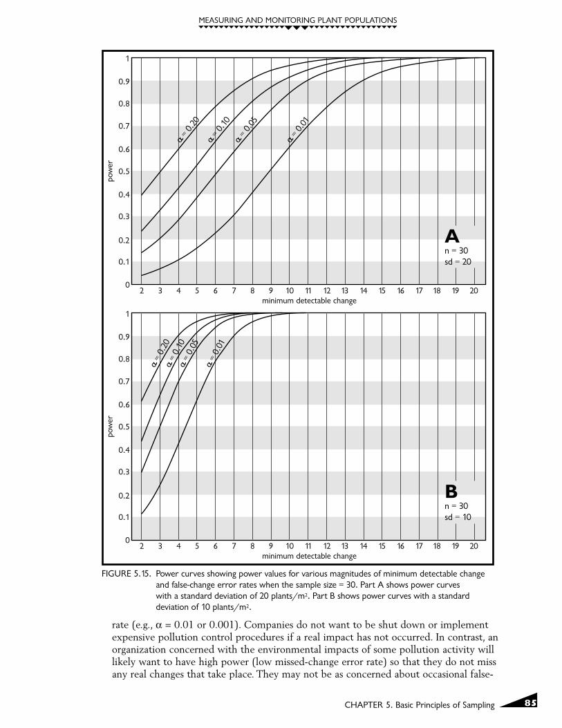
85
MEASURING AND MONITORING PLANT POPULATIONS
CHAPTER 5. Basic Principles of Sampling
rate (e.g., α = 0.01 or 0.001). Companies do not want to be shut down or implementexpensive pollution control procedures if a real impact has not occurred. In contrast, anorganization concerned with the environmental impacts of some pollution activity willlikely want to have high power (low missed-change error rate) so that they do not missany real changes that take place. They may not be as concerned about occasional false-
0
0.1
0.2
0.3
0.4
0.5
0.6
0.7
0.8
0.9
1
2 3 4 5 6 7 8 9 10 11 12 13 14minimum detectable change
pow
er
15 16 17 18 19 20
An = 30sd = 20
0
0.1
0.2
0.3
0.4
0.5
0.6
0.7
0.8
0.9
1
2 3 4 5 6 7 8 9 10 11 12 13 14minimum detectable change
pow
er
15 16 17 18 19 20
= 0.
20
= 0.
10
= 0.
05
= 0.
01
= 0.
20=
0.10
= 0.
05
= 0.
01
Bn = 30sd = 10
FIGURE 5.15. Power curves showing power values for various magnitudes of minimum detectable changeand false-change error rates when the sample size = 30. Part A shows power curveswith a standard deviation of 20 plants/m2. Part B shows power curves with a standarddeviation of 10 plants/m2.

MEASURING AND MONITORING PLANT POPULATIONS
86 CHAPTER 5. Basic Principles of Sampling
change errors (which would result in additional pollution control efforts even though realchanges did not take place).
Missed-change errors may be as costly or more costly than false-change errors in environ-mental monitoring studies (Toft and Shea 1983; Peterman 1990; Fairweather 1991). A false-change error may lead to the commitment of more time, energy, and people, but probablyonly for the short period of time until the mistake is discovered (Simberloff 1990). In con-trast, a missed-change error, as a result of a poor study design, may lead to a false sense ofsecurity until the extent of the damages are so extreme that they show up in spite of a poorstudy design (Fairweather 1991). In this case, rectifying the situation and returning thesystem to its preimpact condition could be costly. For this reason, you may want to set equalfalse-change and missed-change error rates or even consider setting the missed-change errorrate lower than the false-change error rate (Peterman 1990; Fairweather 1991).
There are many historical examples of costly missed-change errors in environmental moni-toring. For example, many fish population monitoring studies have had low power to detectbiologically meaningful declines so that declines were not detected until it was too late andentire populations crashed (Peterman 1990). Some authors advocate the use of somethingthey call the "precautionary principle" (Peterman and M'Gonigle 1992). They argue that, insituations where there is low power to detect biologically meaningful declines in some envi-ronmental parameter, management actions should be prescribed as if the parameter had actu-ally declined. Similarly, some authors prefer to shift the burden of proof in situations wherethere might be an environmental impact from environmental protection interests to indus-try/development interests (Peterman 1990; Fairweather 1991). They argue that a conservativemanagement strategy of "assume the worst until proven otherwise" should be adopted. Underthis strategy, developments that may negatively impact the environment should not proceeduntil the proponents can demonstrate, with high power, a lack of impact on the environment.
7. Why has statistical power been ignored for so long?It is not clear why missed-change errors, power, and minimum detectable change size havetraditionally been ignored. Perhaps researchers have not been sufficiently exposed to the ideaof missed-change errors. Most introductory texts and statistics courses deal with the materialonly briefly. Computer packages for power analysis have only recently become available.Perhaps people have not realized the potentially high costs associated with making missed-change errors. Perhaps researchers have not understood how understanding power canimprove their work.
The issue of power and missed-change errors has gained a lot of attention in recent years. Aliterature review in the 1980’s would not have turned up many articles dealing with statisticalpower issues. A literature review today would turn up dozens of articles in many disciplinesfrom journals all over the world (see Peterman 1990 and Fairweather 1991 for good reviewpapers on statistical power). Journal editors may soon start requiring that power analysisinformation be reported for all nonsignificant results (Peterman 1990). There may also besome departure from the strict adherence to the 0.05 significance level (Peterman 1990;Fairweather 1991).
8. Use of prior power analysis during study designPower analysis can be useful during both the design of monitoring studies and in the inter-pretation of monitoring results. The former is sometimes called "prior power analysis,"whereas the latter is sometimes called "post-hoc power analysis" (Fairweather 1991). Post-hocpower analysis is covered in Chapter 11.

87
MEASURING AND MONITORING PLANT POPULATIONS
CHAPTER 5. Basic Principles of Sampling
The use of power analysis during the design and planning of monitoring studies providesvaluable information that can help avoid monitoring failures. Once some preliminary or pilotdata have been gathered, or if some previous years' monitoring data are available, poweranalysis can be used to evaluate the adequacy of the sampling design. Prior power analysis canbe done in several different ways. All are based upon the power function described earlier:
Power = a function of (s, n, MDC, and α)
The power of a particular sampling design can be evaluated by plugging sample standarddeviation, sample size, the desired MDC, and an acceptable false-change error rate, intoequations or computer programs (Appendix 16) and solving for power. If the power to detecta biologically important change turns out to be quite low (high probability of a missed-change error), then the sampling design can be modified to try to achieve higher power.
Alternatively, a desired power level can be specified and the terms in the power function canbe rearranged to solve for sample size. This will give you assurance that your study designwill succeed in being able to detect a certain magnitude of change at the specified power andfalse-change error rate. This is the format for the sample size equations that are discussed inChapter 7 and presented in Appendix 7.
Still another way to do prior power analysis is to specify a desired power level and a particu-lar sample size and then rearrange the terms in the power function to solve for the MDC(Rotenberry and Wiens 1985; Cohen 1988). If the MDC is unacceptably large, then attemptsshould be made to improve the sampling design. If these efforts fail, then the decision mustbe made to either live with the large MDC or to reject the sampling design and perhapsconsider an alternative monitoring approach.
The main advantage of prior power analysis is that it allows the adequacy of the samplingdesign to be evaluated at an early stage in the monitoring process. It is much better to learnthat a particular design has a low power at a time when modifications can easily be madethan it is to learn of low power after many years of data have already been gathered. Theimportance of specifying acceptable levels of false-change and missed-change errors alongwith the magnitude of change that you want to be able to detect is covered in Chapter 6 thenext chapter, which introduces sampling objectives.
Literature CitedBrewer, J. K. 1972. On the power of statistical tests in the American Educational Research
Journal. American Educational Research Journal 9: 391-401.
Cohen, J. 1988. Statistical power analysis for the behavioral sciences. 2nd edition. Hillsdale, N. J.Lawrence Erlbaum Associates.
Fairweather, P. G. 1991. Statistical power and design requirements for environmental monitoring.Australian Journal of Marine and Freshwater Research 42: 555-567.
Hayes, J. P. 1987. The positive approach to negative results in toxicology studies. Ecotoxicologyand Environmental Safety 14: 73-77.
McCall, C. H. 1982. Sampling and statistics handbook for research. Ames, IA: The Iowa StateUniversity Press.

MEASURING AND MONITORING PLANT POPULATIONS
88 CHAPTER 5. Basic Principles of Sampling
Peterman, R. M. 1990. Statistical power analysis can improve fisheries research and manage-ment. Canadian Journal of Fisheries and Aquatic Sciences. 47: 2-15.
Peterman, R. M.; M'Gognigle. M. 1992. Statistical power analysis and the precautionary principle.Marine Pollution Bulletin. 24(5): 231-234.
Rotenberry, J. T.; Wiens J. A. 1985. Statistical power analysis and community-wide patterns.American Naturalist. 125: 164-168.
Simberloff, D. 1990. Hypotheses, errors, and statistical assumptions. Herpetelogica. 46: 351-357.
Toft, C. A.; P. J. Shea. 1983. Detecting community-wide patterns: estimating power strengthensstatistical inference. American Naturalist. 122: 618-625.
Zar, J. H. 1996. Biostatistical Analysis. Englewood Cliffs, N.J. Jersey: Prentice-Hall, Inc.