Measuring the Performance of a Distributed

Quota Enforcement System for Spam Control

by

John Dalbert Zamfirescu-Pereira

Submitted to the Department of Electrical Engineering and Computer

Sciencein partial fulfillment of the requirements for the degree of

Master of Engineering in Electrical Engineering and Computer Science

at the

MASSACHUSETTS INSTITUTE OF TECHNOLOGY

June 2006

c© John Dalbert Zamfirescu-Pereira, MMVI. All rights reserved.

The author hereby grants to MIT permission to reproduce anddistribute publicly paper and electronic copies of this thesis document

in whole or in part.

Author . . . . . . . . . . . . . . . . . . . . . . . . . . . . . . . . . . . . . . . . . . . . . . . . . . . . . . . . . . . . . .

Department of Electrical Engineering and Computer ScienceMay 23, 2006

Certified by. . . . . . . . . . . . . . . . . . . . . . . . . . . . . . . . . . . . . . . . . . . . . . . . . . . . . . . . . .Hari Balakrishnan

ProfessorThesis Supervisor

Accepted by . . . . . . . . . . . . . . . . . . . . . . . . . . . . . . . . . . . . . . . . . . . . . . . . . . . . . . . . .Arthur C. Smith

Chairman, Department Committee on Graduate Theses

2

Measuring the Performance of a Distributed Quota

Enforcement System for Spam Control

by

John Dalbert Zamfirescu-Pereira

Submitted to the Department of Electrical Engineering and Computer Scienceon May 23, 2006, in partial fulfillment of the

requirements for the degree ofMaster of Engineering in Electrical Engineering and Computer Science

Abstract

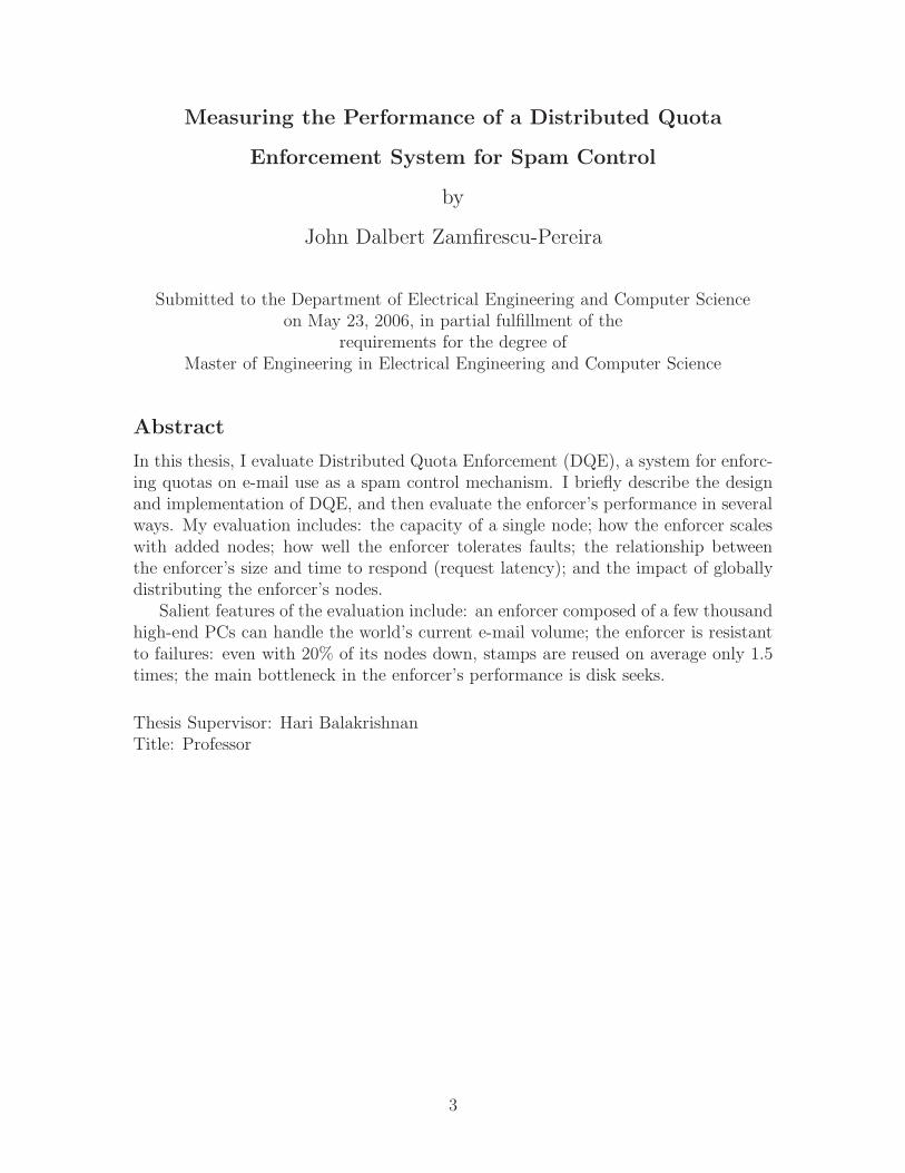
In this thesis, I evaluate Distributed Quota Enforcement (DQE), a system for enforc-ing quotas on e-mail use as a spam control mechanism. I briefly describe the designand implementation of DQE, and then evaluate the enforcer’s performance in severalways. My evaluation includes: the capacity of a single node; how the enforcer scaleswith added nodes; how well the enforcer tolerates faults; the relationship betweenthe enforcer’s size and time to respond (request latency); and the impact of globallydistributing the enforcer’s nodes.

Salient features of the evaluation include: an enforcer composed of a few thousandhigh-end PCs can handle the world’s current e-mail volume; the enforcer is resistantto failures: even with 20% of its nodes down, stamps are reused on average only 1.5times; the main bottleneck in the enforcer’s performance is disk seeks.

Thesis Supervisor: Hari BalakrishnanTitle: Professor

3

4

Acknowledgments

My first thanks go to my supervisor Hari Balakrishnan, for helping me realize that

hard work is very rewarding; if there is anything I will take away from my experience

at CSAIL, that is it. Hari has—through his example—shown me new ways of looking

at problems, and his research ability has been (and will continue to be) a source of

inspiration for me.

I would also like to thank Michael Walfish, my partner in crime. First, for his

help in getting my technical writing into shape; second, for pointing me in the right

direction on numerous occasions; and third, for helping me realize that good work

takes time.

This work would have been much more difficult without the Emulab testbed; my

thanks go out to everyone involved with the Flux Research Group at the University

of Utah. Thank you all!

Finally, I would like to thank my parents, and especially my mother, for their help

in bringing me where I am today!

5

6

Contents

1 Introduction 13

1.1 Quota System Requirements . . . . . . . . . . . . . . . . . . . . . . . 14

1.2 DQE Evaluation . . . . . . . . . . . . . . . . . . . . . . . . . . . . . 15

1.3 Organization . . . . . . . . . . . . . . . . . . . . . . . . . . . . . . . 16

2 Distributed Quota Enforcement for Spam Control 19

2.1 DQE Architecture . . . . . . . . . . . . . . . . . . . . . . . . . . . . . 19

2.2 The Enforcer . . . . . . . . . . . . . . . . . . . . . . . . . . . . . . . 20

2.2.1 Replication . . . . . . . . . . . . . . . . . . . . . . . . . . . . 21

2.2.2 get and put . . . . . . . . . . . . . . . . . . . . . . . . . . . 22

2.2.3 Avoiding “Distributed Livelock” . . . . . . . . . . . . . . . . . 23

2.2.4 Cluster and Wide-area Deployments . . . . . . . . . . . . . . 25

3 Implementation and Evaluation of the Enforcer 27

3.1 Implementation . . . . . . . . . . . . . . . . . . . . . . . . . . . . . . 27

3.1.1 DQE Client Software . . . . . . . . . . . . . . . . . . . . . . . 27

3.1.2 Enforcer Node Software . . . . . . . . . . . . . . . . . . . . . 28

3.2 Evaluation . . . . . . . . . . . . . . . . . . . . . . . . . . . . . . . . . 28

3.2.1 Environment . . . . . . . . . . . . . . . . . . . . . . . . . . . 29

3.2.2 Fault Tolerance . . . . . . . . . . . . . . . . . . . . . . . . . . 29

3.2.3 Single-node Microbenchmarks . . . . . . . . . . . . . . . . . . 31

3.2.4 Capacity of the Enforcer . . . . . . . . . . . . . . . . . . . . . 32

3.2.5 Estimating the Enforcer Size . . . . . . . . . . . . . . . . . . . 35

7

3.2.6 Clustered and Wide-area Enforcers . . . . . . . . . . . . . . . 38

3.2.7 Avoiding “Distributed Livelock” . . . . . . . . . . . . . . . . . 39

3.2.8 Limitations . . . . . . . . . . . . . . . . . . . . . . . . . . . . 40

4 Trade-offs in “Distributed Livelock Avoidance” 41

4.1 Repeated Use of a Single Stamp . . . . . . . . . . . . . . . . . . . . . 42

4.1.1 test = set . . . . . . . . . . . . . . . . . . . . . . . . . . . . 42

4.1.2 test ≺ set . . . . . . . . . . . . . . . . . . . . . . . . . . . . 43

4.1.3 test ≻ set . . . . . . . . . . . . . . . . . . . . . . . . . . . . 43

4.2 Stamps Used At Most Twice . . . . . . . . . . . . . . . . . . . . . . . 44

4.2.1 test = set . . . . . . . . . . . . . . . . . . . . . . . . . . . . 44

4.2.2 test ≺ set . . . . . . . . . . . . . . . . . . . . . . . . . . . . 44

4.2.3 test ≻ set . . . . . . . . . . . . . . . . . . . . . . . . . . . . 45

4.3 Prioritizing Based on Content . . . . . . . . . . . . . . . . . . . . . . 46

5 Related Work 49

5.1 Spam Control . . . . . . . . . . . . . . . . . . . . . . . . . . . . . . . 49

5.2 Related Distributed Systems . . . . . . . . . . . . . . . . . . . . . . . 51

5.3 Related Measurement Work . . . . . . . . . . . . . . . . . . . . . . . 53

6 Conclusions 55

A Relating Microbenchmarks to System Performance 57

B Exact Expectation Calculation in “Crashed” Experiment 63

8

List of Figures

2-1 DQE architecture. . . . . . . . . . . . . . . . . . . . . . . . . . . . . 20

2-2 Enforcer design . . . . . . . . . . . . . . . . . . . . . . . . . . . . . . 21

2-3 Pseudo-code for test and set . . . . . . . . . . . . . . . . . . . . . . 22

2-4 Pseudo-code for get and put . . . . . . . . . . . . . . . . . . . . . . 24

3-1 Effect of “bad” nodes . . . . . . . . . . . . . . . . . . . . . . . . . . . 30

3-2 32-node enforcer capacity . . . . . . . . . . . . . . . . . . . . . . . . . 35

3-3 Enforcer scalability . . . . . . . . . . . . . . . . . . . . . . . . . . . . 36

3-4 Link latencies in the Abilene PoP network . . . . . . . . . . . . . . . 38

3-5 Effect of livelock avoidance . . . . . . . . . . . . . . . . . . . . . . . . 40

4-1 Comparing livelock priorities . . . . . . . . . . . . . . . . . . . . . . . 46

9

10

List of Tables

3.1 Single-node performance . . . . . . . . . . . . . . . . . . . . . . . . . 32

3.2 Enforcer size estimate . . . . . . . . . . . . . . . . . . . . . . . . . . 35

3.3 Enforcer Size vs. Latency . . . . . . . . . . . . . . . . . . . . . . . . 37

A.1 RPCs generated by a test . . . . . . . . . . . . . . . . . . . . . . . . 58

A.2 set circumstances . . . . . . . . . . . . . . . . . . . . . . . . . . . . 59

A.3 Reused test circumstances . . . . . . . . . . . . . . . . . . . . . . . 59

A.4 Values of C(Ai, Bj) . . . . . . . . . . . . . . . . . . . . . . . . . . . . 60

A.5 Probabilities P(Bj | Ai) . . . . . . . . . . . . . . . . . . . . . . . . . . 60

11

12

Chapter 1

Introduction

By industry accounts, spam—unsolicited commercial e-mail—constitutes some 65%

of the world’s total e-mail volume [9]. Several solutions to the spam problem have

been proposed, some of which are in use (e.g., context-based filters such as Spa-

mAssassin [54]) and some which are not (e.g., quota systems, like the Penny Black

project [45]). As of 2006, context- and content-based filters are by far the more

popular anti-spam measure. However, while filters do provide temporary relief from

spam, they have one important shortcoming: filters are inherently limited by their

potential to falsely identify legitimate mail as spam, which reduces e-mail’s reliability

as a communications medium. A quota system addresses this shortcoming (but not

without its own problems, of course), by fighting spam on a different level: a quota

scheme simply prevents individuals and organizations from sending more than their

fair share of e-mail.

In a quota system, all participants are assigned a quota of stamps. A message

sender then attaches one of these stamps to each e-mail, which the message receiver

tests at a quota enforcer to verify that it has not already been used. A “fresh” (unused)

stamp is guaranteed to bring its associated message to the receiver’s attention. The

hope is that by allocating everyone a reasonable quota, legitimate users will not be

substantially constrained in their ability to send mail, but spammers will no longer

be able to send the volumes of messages required to be profitable.

Note that quota enforcement is a different problem from quota allocation; the

13

latter is a social problem, which we don’t purport to solve, while the former is a

technical one and the focus of this work—in fact, our intent is to show that the

challenges in quota enforcement can be overcome.

Our group has designed, implemented, and evaluated Distributed Quota Enforce-

ment (DQE); my contribution to this project, and indeed my main focus in this thesis,

is the experimental evaluation of DQE. A majority of the work presented here has

already appeared in print in [59]; text in this document that appears in that paper is

so indicated.

1.1 Quota System Requirements

We begin by discussing some of the motivations behind DQE. In addition to restoring

reliability to e-mail by preventing false positives, a quota-based system must address

two sets of concerns. The first set apply to the manner in which clients communicate

with the quota enforcer: First, our ban on false positives means clients must never

be led to believe that a message is spam when it is not. As we assume that a reused

stamp indicates spam, a fresh stamp must never appear used. Second, clients must

not be required to trust the enforcer, so that the enforcer need not be run by a

central authority. Finally, the quota system should not impact the semantics of e-

mail, specifically, enforcer queries should not identify senders, and stamps should not

be an irrefutable testament that one party sent a particular message to another.

The second set of concerns apply to the quota enforcer itself. From [59]:

Scalability The enforcer must scale to current and future e-mail vol-

umes. Studies estimate that 80-90 billion e-mails will be sent daily this

year [31, 47]. (We admit that we have no way to verify these claims.)

We set an initial target of 100 billion daily messages (an average of about

1.2 million stamp checks per second) and strive to keep pace with future

growth. To cope with these rates, the enforcer must be composed of many

hosts.

14

Fault-tolerance Given the required number of hosts, it is highly likely

that some subset will experience crash faults (e.g., be down) or Byzantine

faults (e.g., become subverted). The enforcer should be robust to these

faults. In particular, it should guarantee no more than a small amount of

stamp reuse, despite such failures.

High throughput To control management and hardware costs, we

wish to minimize the required number of machines, which requires maxi-

mizing throughput.

Attack-resilience Spammers will have a strong incentive to cripple

the enforcer; it should thus resist denial-of-service (DoS) and resource

exhaustion attacks.

Mutually untrusting nodes In both federated and monolithic en-

forcer organizations, nodes could be compromised. In the federated case,

even when the nodes are uncompromised, they may not trust each other.

Thus, in either case, besides being untrusted (by clients), nodes should

also be untrusting (of other nodes), even as they do storage operations for

each other.

These concerns guide the design of DQE. A full treatment of how these concerns

have influenced our design decisions is beyond the scope of this thesis. However, for

completeness, I summarize the relevant features of DQE’s design in Chapter 2.

1.2 DQE Evaluation

Some of the requirements that drive DQE’s construction also present an avenue for

evaluation. In this thesis, we1 evaluate:

1Though the evaluation of DQE presented here is primarily driven by my own work, all parts ofDQE are the result of a collaborative effort; thus, the narrative uses “we” instead of “I” to describecollective work.

15

Scalability We first evaluate the performance of a single-node enforcer. Then we

evaluate how performance scales with successively larger enforcers. The ideal behavior

is a linear increase in performance as the enforcer grows; the observed behavior very

nearly matches this ideal.

Fault-tolerance Next, we evaluate how well the enforcer prevents stamp reuse in

the presence of node failures; a conservative upper bound suggests that the enforcer

can keep stamp use as low as 1.3 uses/stamp, even if 10% of the node are “bad”.

High throughput We also verify that an enforcer is capable of handling global

e-mail volumes, without requiring an unreasonable number of nodes; a simple calcu-

lation indicates that an enforcer of several thousand nodes would suffice.

Size/latency trade-off Here we investigate the relationship between an enforcer’s

size and the time required for it to respond to clients’ requests; an increased tolerance

for latency in responses allows a smaller enforcer.

Wide-area distribution Finally, we investigate the differences between a clus-

tered enforcer and one whose nodes are spread across several different organizations,

possibly with global distribution; we see that this distribution has limited effects on

throughput, but does increase response latency.

In addition to these meeting these requirements, the design of DQE includes sev-

eral interesting technical solutions for problems we encountered while implementing

the enforcer. Included among these is a scheme to avoid “distributed livelock” by pri-

oritizing certain packet classes over others; we present an analysis of the implemented

scheme and a number of alternative prioritizations as well.

1.3 Organization

The remainder of this document is organized as follows: Chapter 2 describes the

features of DQE’s design that are relevant to the experimental evaluation; Chapter 3

16

presents the experimental evaluation itself; in Chapter 4 we consider several “dis-

tributed livelock” avoidance schemes; Chapter 5 presents a summary of related work;

finally, Chapter 6 presents conclusions.

17

18

Chapter 2

Distributed Quota Enforcement for

Spam Control

DQE can be logically split into two parts. The first is the external interface, consisting

of quota allocation and stamp creation and verification. The second is the enforcer

itself. In this chapter, I briefly summarize the design of DQE.1

2.1 DQE Architecture

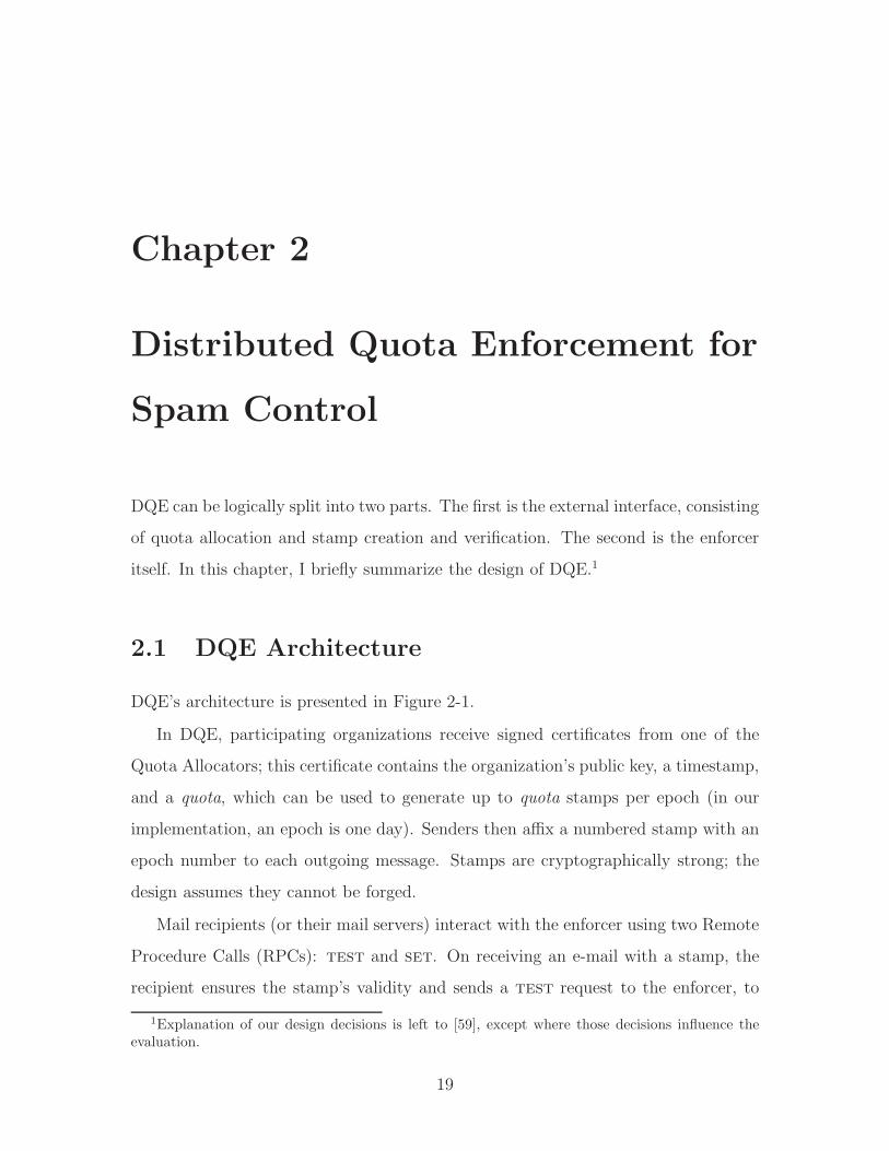
DQE’s architecture is presented in Figure 2-1.

In DQE, participating organizations receive signed certificates from one of the

Quota Allocators; this certificate contains the organization’s public key, a timestamp,

and a quota, which can be used to generate up to quota stamps per epoch (in our

implementation, an epoch is one day). Senders then affix a numbered stamp with an

epoch number to each outgoing message. Stamps are cryptographically strong; the

design assumes they cannot be forged.

Mail recipients (or their mail servers) interact with the enforcer using two Remote

Procedure Calls (RPCs): test and set. On receiving an e-mail with a stamp, the

recipient ensures the stamp’s validity and sends a test request to the enforcer, to

1Explanation of our design decisions is left to [59], except where those decisions influence theevaluation.

19

EnforcerQuota

Allocators

Outgoing Mail Server

Portal

Incoming Mail Server

Certificatewith quota

(or mail sender) (or mail recipient)

Mail with certificate and stamp

1. TEST3. SET

2. RESP

Client

Figure 2-1: DQE architecture.

determine whether the enforcer has seen a fingerprint of the stamp. If the response

is “not found”, the recipient sends a set request to the enforcer, presenting a fin-

gerprint of the stamp to be stored. The enforcer itself stores a mapping from the

stamp’s postmark—hash(hash(stamp))—to its fingerprint—hash(stamp); map-

pings are stored for the current and previous epochs. To prevent a malicious node from

falsely claiming it has seen a stamp, a test queries the postmark, and the enforcer

must respond with the corresponding pre-image under hash (i.e., the fingerprint of

the stamp).

2.2 The Enforcer

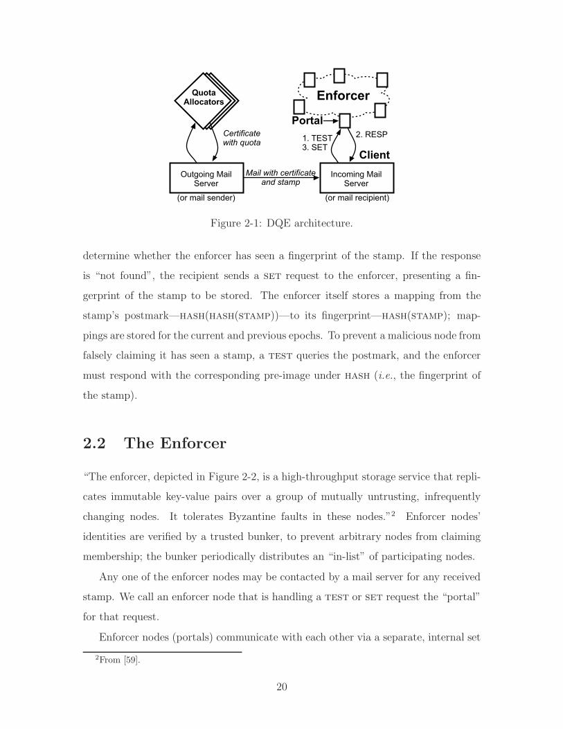
“The enforcer, depicted in Figure 2-2, is a high-throughput storage service that repli-

cates immutable key-value pairs over a group of mutually untrusting, infrequently

changing nodes. It tolerates Byzantine faults in these nodes.”2 Enforcer nodes’

identities are verified by a trusted bunker, to prevent arbitrary nodes from claiming

membership; the bunker periodically distributes an “in-list” of participating nodes.

Any one of the enforcer nodes may be contacted by a mail server for any received

stamp. We call an enforcer node that is handling a test or set request the “portal”

for that request.

Enforcer nodes (portals) communicate with each other via a separate, internal set

2From [59].

20

idC IPC

idB IPB

IPAidAindex

in-listnode A

B

C

D

TEST(k)

SET(k,v)

GET(k)

GET(k)

GET(k)

{idB, idC, idD}k

PUT(k,v)

Bunker in-list

in-list

Figure 2-2: Enforcer design. A test causes multiple gets; a set causes one put.Here, A is the portal. The ids are in a circular identifier space with the identifiersdetermined by the bunker.

of RPCs: get and put. They treat clients’ test and set requests as queries on

key-value pairs, that is, as test(k) and set(k, v), where k = hash(v). Portals then

send get(k) and put(k, v) requests to other enforcer nodes to implement test and

set.

Responsibility for storing a particular stamp is distributed across r enforcer nodes.

We call these nodes the “assigned” nodes for a particular stamp; they are determined

by the stamp, using a consistent hashing [34] algorithm. Any of the assigned nodes

for a stamp may store its associated key-value pair.

In response to a test(k) request, a portal invokes a get(k) request at k’s r

assigned nodes, one at a time. If any of the nodes returns “found” with a v such

that v = hash(k), the portal stops and returns “found” to the client. Otherwise, the

portal simply returns “not found” to the client. In response to a set(k, v) request,

the portal chooses one of the r nodes at random and issues it a put(k, v) request.

Pseudo-code for test and set is given in Figure 2-3.

2.2.1 Replication

A major factor in the ability of the enforcer to withstand faults is the choice of

replication factor, r. We assume for this analysis that nodes do not abuse their role

as “portal”.

21

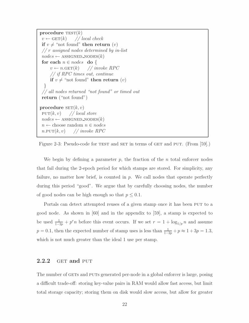
procedure test(k)v ← get(k) // local checkif v 6= “not found” then return (v)// r assigned nodes determined by in-listnodes← assigned nodes(k)for each n ∈ nodes do {

v ← n.get(k) // invoke RPC// if RPC times out, continueif v 6= “not found” then return (v)

}// all nodes returned “not found” or timed outreturn (“not found”)

procedure set(k, v)put(k, v) // local storenodes← assigned nodes(k)n← choose random n ∈ nodesn.put(k, v) // invoke RPC

Figure 2-3: Pseudo-code for test and set in terms of get and put. (From [59].)

We begin by defining a parameter p, the fraction of the n total enforcer nodes

that fail during the 2-epoch period for which stamps are stored. For simplicity, any

failure, no matter how brief, is counted in p. We call nodes that operate perfectly

during this period “good”. We argue that by carefully choosing nodes, the number

of good nodes can be high enough so that p ≤ 0.1.

Portals can detect attempted reuses of a given stamp once it has been put to a

good node. As shown in [60] and in the appendix to [59], a stamp is expected to

be used 11−2p

+ prn before this event occurs. If we set r = 1 + log1/p n and assume

p = 0.1, then the expected number of stamp uses is less than 11−2p

+ p ≈ 1+3p = 1.3,

which is not much greater than the ideal 1 use per stamp.

2.2.2 get and put

The number of gets and puts generated per-node in a global enforcer is large, posing

a difficult trade-off: storing key-value pairs in RAM would allow fast access, but limit

total storage capacity; storing them on disk would slow access, but allow for greater

22

storage.

DQE uses a “key-value store” data structure that combines an in-RAM component

(a hash map and overflow table, collectively called the “index”) with an on-disk

component (that stores key-value pairs). A queried key is first looked up in the index;

if the key has been put, that lookup returns a pointer to the disk block storing the

the key-value pair. A put request results in insertion of the key into a hash table

(or an overflow table in the event of a collision), and storage of the key-value pair on

disk.

The key-value store has several attractive properties: puts are fast; the store has

a small memory footprint, storing 5.3 bytes per stamp instead of the stamp’s original

40 bytes; and the store is almost always able to respond to “not found” requests

quickly, that is, without accessing the disk, though “found” requests require a disk

seek and are thus “slow”. The exact interaction between get and put requests and

the key-value store is presented in Figure 2-4.

2.2.3 Avoiding “Distributed Livelock”

One key requirement for the enforcer is that performance not degrade under load,

where load may be the result of heavy legitimate system use or attackers’ spurious

requests. In fact, in an early implementation, our enforcer’s capacity, as measured by

the total number of correct responses to test requests, did worsen under load. In

response to this degradation, we made several changes to the libasync library we use

to support our RPC protocol. This section describes those changes.

First observe that all of the work enforcer nodes perform is caused by packets as-

sociated with RPCs from clients or other nodes, and that these packets can be divided

into three classes: (1) tests and sets from clients comprise “external” requests; (2)

gets and puts from other enforcer nodes comprise “internal” requests; and (3) get

and put responses from other enforcer nodes comprise internal responses.

Overload—when the CPU is unable to do the work caused by all arriving packets—

will result in some packets being dropped (we call those that are not dropped “admit-

ted”). To maximize correct test responses, nodes must ensure successful completion

23

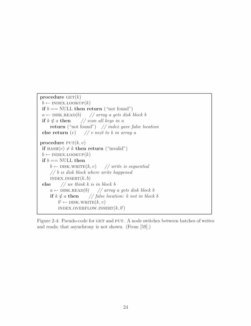
procedure get(k)b← index.lookup(k)if b == NULL then return (“not found”)a← disk.read(b) // array a gets disk block bif k /∈ a then // scan all keys in a

return (“not found”) // index gave false locationelse return (v) // v next to k in array a

procedure put(k, v)if hash(v) 6= k then return (“invalid”)b← index.lookup(k)if b == NULL then

b← disk.write(k, v) // write is sequential// b is disk block where write happenedindex.insert(k, b)

else // we think k is in block ba← disk.read(b) // array a gets disk block bif k /∈ a then // false location: k not in block b

b′ ← disk.write(k, v)index.overflow.insert(k, b′)

Figure 2-4: Pseudo-code for get and put. A node switches between batches of writesand reads; that asynchrony is not shown. (From [59].)

24

of the get and put operations generated by tests. To maximize the number of

completed get and put requests, nodes must ensure that, under heavy load, the

responses to those get and put requests that are admitted are then admitted them-

selves by the requesting portal. Note that if a node admits a get request when it

could have admitted a get response instead, the work put in to that response is

wasted. Thus, to maximize successfully completed gets and puts, nodes prioritize

the three packet classes, so that internal responses (3) are preferred over internal

requests (2), in turn preferred over external requests (1).

In our early implementations, nodes did not prioritize, and instead served the

three classes in a round-robin manner. Round-robin admittance meant that packets

were dropped from all three classes, causing two problems: first, many get requests

and responses were dropped, resulting in unsuccessful gets and thus incorrect test

responses; second, additional test requests were admitted at the expense of get

requests and responses, causing the enforcer to over-commit to clients. As noted

in [59]: “The combination is distributed livelock: nodes spent cycles on tests and

sets and meanwhile dropped get and put requests and responses from other nodes.”

The astute reader may realize that prioritizing the three packet classes does little

more than cause enforcer nodes to drop packets from the beginning of the “distributed

pipeline” formed by the test→get request→get response RPC sequence. The

overriding principle is that a system should drop those packets in which it has invested

the least amount of work; in the enforcer’s case, those packets are the ones in class

(1): test and set requests.

Note that the “distributed pipeline” formed by RPCs can be constructed in several

ways: above, tests and sets are considered to be in the same class, but a test may

also be considered to come before the set in the pipeline. Different pipelines suggest

different prioritization schemes; I explore some of these alternatives in Chapter 4.

2.2.4 Cluster and Wide-area Deployments

Recall from the requirements laid out in Chapter 1 that the enforcer should support

a range of deployments. One such deployment, and indeed the focus of Chapter 3, is

25

a “monolithic” enforcer whose nodes are located in a single cluster. In a monolithic

enforcer, all nodes are on a single LAN. This LAN can be provisioned with enough

bandwidth to handle peak rates without congestion, and a simple UDP-based protocol

suffices for inter-node communication.

Given the thousands of nodes (see §3.2.5) a global enforcer would require, a “feder-

ated” enforcer—with nodes either individually owned by participating organizations

or grouped in clusters around the globe—may be a more realistic deployment. In

a federated enforcer, a substantial fraction of internal traffic—gets and puts—will

travel over commodity Internet links. For the enforcer to “play well” with existing

network traffic, some care must be taken to ensure that heavy load does not unreason-

ably degrade those links. A naıve option is to use pairwise TCP connections between

enforcer nodes, but TCP incurs significant overhead providing semantics the enforcer

does not need: guaranteed and in-order delivery.

To avoid TCP’s overhead, the enforcer has the option of using a TCP-friendly

datagram protocol, the Datagram Congestion Control Protocol (DCCP) [35] for com-

munication between nodes. DCCP is a natural choice, providing the minimum needed:

congestion control for the unreliable datagram flows the enforcer nodes use to com-

municate with each other.

It is worth noting that the livelock avoidance scheme and congestion control op-

erate at opposite ends of the spectrum. If an enforcer is clustered, it needs livelock

avoidance, but not congestion control; by the same token, a federated enforcer—whose

nodes are connected via relatively low-capacity links—needs congestion control, but

not livelock avoidance.

26

Chapter 3

Implementation and Evaluation of

the Enforcer

In this chapter, I describe the implementation and evaluation of DQE. Most of the

text appearing in §3.2 is taken verbatim from [59].

3.1 Implementation

DQE consists of two parts: the DQE client software, which runs at e-mail senders

and receivers, and the DQE enforcer software.

3.1.1 DQE Client Software

From [59]:

The DQE client software is two Python modules. A sender module is in-

voked by a sendmail hook; it creates a stamp and inserts it in a new

header in the departing message. The receiver module is invoked by

procmail; it checks whether the e-mail has a stamp and, if so, executes

a test RPC over XDR to a portal. Depending on the results (no stamp,

already canceled stamp, forged stamp, etc.), the module adds a header

to the e-mail for processing by filter rules. To reduce client-perceived la-

27

tency, the module first delivers e-mail to the recipient and then, for fresh

stamps, asynchronously executes the set.

3.1.2 Enforcer Node Software

The enforcer is a 5000-line event-driven C++ program that exposes its interfaces via

XDR RPC over UDP or DCCP (configurable at compile time). It uses libasync [41]

and its asynchronous I/O daemon [38]; we modified libasync to implement the livelock

avoidance scheme from §2.2.3, and modified the asynchronous I/O daemon to support

DCCP (see §2.2.4). The enforcer runs under both Linux 2.6 and FreeBSD 5.3; DCCP

requires the use of a custom kernel under Linux and is currently unsupported under

FreeBSD.

3.2 Evaluation

In this section, we evaluate the enforcer experimentally. We first investigate how its

observed fault-tolerance—in terms of the average number of stamp reuses as a function

of the number of faulty machines—matches the analysis in §2.2.1. We next investigate

the capacity of a single enforcer node, measure how this capacity scales with multiple

nodes, and then estimate the number of dedicated enforcer nodes needed to handle

100 billion e-mails per day (our target volume; see §1.1). We next evaluate the livelock

avoidance scheme from §2.2.3. Finally, we investigate the effects of distributing the

enforcer over a wide area.

All of our experiments use the Emulab testbed [21]. Except where noted, these

experiments consist of between one and 64 enforcer nodes connected to a single LAN,

using UDP for inter-node communication.1 The setup models a clustered network

service with a high-speed access link. We additionally run one simulated “wide-area”

experiment and one experiment using DCCP for inter-node communication (both in

§3.2.6).

1We evaluate the enforcer using UDP instead of DCCP simply because UDP communication wasimplemented first.

28

3.2.1 Environment

Each enforcer node runs on a separate Emulab host. To simulate clients and to test

the enforcer under load, we run up to 25 instances of an open-loop tester, U (again,

one per Emulab host). All hosts run Linux FC4 (2.6 kernel) and are Emulab’s “PC

3000s”, which have 3 GHz Xeon processors, 2 GBytes of RAM, 100 Mbit/s Ethernet

interfaces, and 10,000 RPM SCSI disks.

Each U follows a Poisson process to generate tests and selects the portal for each

test uniformly at random. This process models various e-mail servers sending tests

to various enforcer nodes. (As argued in [44], Poisson processes appropriately model a

collection of many random, unrelated session arrivals in the Internet.) The proportion

of reused tests (stamps2 previously set by U) to fresh tests (stamps never set by

U) is configurable. These two test types model an e-mail server receiving a spam or

non-spam message, respectively. In response to a “not found” reply—which happens

either if the stamp is fresh or if the enforcer lost the reused stamp—U issues a set

to the portal it chose for the test.

Our reported experiments run for 12 or 30 minutes. Separately, we ran a 12-hour

test to verify that the performance of the enforcer does not degrade over time.

3.2.2 Fault Tolerance

We first investigate whether failures in the implemented system reflect the analysis.

Recall that this analysis (in §2.2.1, and in detail in [59]’s appendix and in Appendix B)

upper bounds the average number of stamp uses in terms of p, where p is the prob-

ability a node is bad, i.e., that it is ever down while a given stamp is relevant (two

days). Below, we model “bad” with crash faults only (see [59], §4.5 for the relationship

between Byzantine and crash faults).

We run two experiments in which we vary the number of bad nodes. These

experiments measure how often the enforcer fails to “find” stamps it has already

“heard” about because some of its nodes have crashed.

2In this section (§3.2), we often use “stamp” to refer to the key-value pair associated with thestamp.

29

1

1.2

1.4

1.6

1.8

2

25.022.520.017.515.0

Avg

. # u

ses/

stam

p

% nodes bad (40 nodes total)

upper boundcrashed, analytic

crashed, observedchurning, observed

Figure 3-1: Effect of “bad” nodes on stamp reuse for two types of “bad”. Observeduses obey the upper bound from the analysis (see §2.2.1 and [59]’s appendix). Thecrashed case in analyzed exactly in appendix B; the observations track this analysisclosely.

In the first experiment, called crashed, the bad nodes are never up. In the second,

called churning, the bad nodes repeat a 90-second cycle of 45 seconds of down time

followed by 45 seconds of up time. Both experiments run for 30 minutes. The Us

issue tests and sets to the up nodes, as described in §3.2.1. Half the tests are for

fresh stamps, and the other half are for a reuse group—843,750 reused stamps that

are each queried 32 times during the experiment. This group of tests models an

adversary trying to reuse a stamp. The Us count the number of “not found” replies

for each stamp in the reuse group; each such reply counts as a stamp use. We set

n = 40, and the number of bad nodes is between 6 and 10, so p varies between 0.15

and 0.25. For the replication factor (§2.2.1), we set r = 3.

The results are depicted in Figure 3-1. The two “observed” lines plot the average

number of times a stamp in the “reuse group” was used successfully. These obser-

vations obey the model’s least upper bound. This bound, from [59]’s appendix, is

30

1+ 32p+3p2+p3

[40 (1− p)−

(1 + 3

2+ 3)]

and is labeled “upper bound”.3 The crashed

experiment is amenable to an exact expectation calculation. The resulting expres-

sion4 is depicted by the line labeled “crashed, analytic”; it matches the observations

well.

3.2.3 Single-node Microbenchmarks

We now examine the performance of a single-node enforcer. We begin with RAM

and ask how it limits the number of puts. Each key-value pair consumes roughly

5.3 bytes of memory in expectation (see §2.2.2 and [59], §4.2), and each is stored for

two days. Thus, with one GByte of RAM, a node can store slightly fewer than 200

million key-value pairs, which, over two days, is roughly 1100 puts per second. A

node can certainly accept a higher average rate over any given period but must limit

the total number of puts it accepts each day to 100 million for every GByte of RAM.

Our implementation does not currently rate-limit inbound puts.

We next ask how the disk limits gets. (The disk does not bottleneck puts because

writes are sequential and because disk space is ample.) Consider a key k requested

at a node d. We call a get slow if d stores k on disk (if so, d has an entry for k in

its index) and k is not in d’s RAM cache (see §2.2.2 and [59], §4.2). We expect d’s

ability to respond to slow gets to be limited by disk seeks. To verify this belief, an

instance of U sends tests and sets at a high rate to a single-node enforcer, inducing

local gets and puts. The node runs with its cache of key-value pairs disabled. The

node responds to an average of 400 slow gets per second (measured over 5-second

intervals, with standard deviation less than 10% of the mean). This performance

agrees with our disk benchmark utility, which does random access reads in a tight

loop.

We next consider fast gets, which are gets on keys k for which the node has k

3We take n = 40(1− p) instead of n = 40 because, as mentioned above, the Us issue tests andsets only to the “up” nodes.

4The expression, with m = 40(1−p), is (1−p)3(1)+3p2(1−p)α+3p(1−p)2β+p3m(

1−(

m−1m

)32)

.

α is∑

m

i=1 i(

23

)i−1 1m

(1 + m−i

3

), and β is

∑m−1i=1 i

(13

)i−1 m−i

m(m−1)

(2 + 2

3 (m− (i + 1))). See ap-

pendix B for a derivation.

31

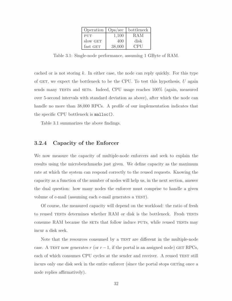
Operation Ops/sec bottleneckput 1,100 RAMslow get 400 diskfast get 38,000 CPU

Table 3.1: Single-node performance, assuming 1 GByte of RAM.

cached or is not storing k. In either case, the node can reply quickly. For this type

of get, we expect the bottleneck to be the CPU. To test this hypothesis, U again

sends many tests and sets. Indeed, CPU usage reaches 100% (again, measured

over 5-second intervals with standard deviation as above), after which the node can

handle no more than 38,000 RPCs. A profile of our implementation indicates that

the specific CPU bottleneck is malloc().

Table 3.1 summarizes the above findings.

3.2.4 Capacity of the Enforcer

We now measure the capacity of multiple-node enforcers and seek to explain the

results using the microbenchmarks just given. We define capacity as the maximum

rate at which the system can respond correctly to the reused requests. Knowing the

capacity as a function of the number of nodes will help us, in the next section, answer

the dual question: how many nodes the enforcer must comprise to handle a given

volume of e-mail (assuming each e-mail generates a test).

Of course, the measured capacity will depend on the workload: the ratio of fresh

to reused tests determines whether RAM or disk is the bottleneck. Fresh tests

consume RAM because the sets that follow induce puts, while reused tests may

incur a disk seek.

Note that the resources consumed by a test are different in the multiple-node

case. A test now generates r (or r−1, if the portal is an assigned node) get RPCs,

each of which consumes CPU cycles at the sender and receiver. A reused test still

incurs only one disk seek in the entire enforcer (since the portal stops geting once a

node replies affirmatively).

32

32-node experiments We first determine the capacity of a 32-node enforcer. To

emulate the per-node load of a several thousand-node deployment, we set r = 5

(which we get because, from §2.2.1, r = 1 + log1/p n; we take p = 0.1 and n = 8000,

which is the upper bound in §3.2.5).

We run two groups of experiments in which 20 instances of U send half fresh and

half reused tests at various rates to this enforcer. In the first group, called disk, the

nodes’ key-value caches are disabled, forcing a disk seek for every affirmative get

(§2.2.2). In the second group, called CPU, we enable the caches and set them large

enough that stamps will be stored in the cache for the duration of the experiment.

The first group of experiments is fully pessimistic and models a disk-bound workload

whereas the second is (unrealistically) optimistic and models a workload in which RPC

processing is the bottleneck. We ignore the RAM bottleneck in these experiments

but consider it at the end of the section.

Each node reports how many reused tests it served over the last 5 seconds (if

too many arrive, the node’s kernel silently drops). Each experiment run happens at a

different test rate. For each run, we produce a value by averaging together all of the

nodes’ 5-second reports. Figure 3-2 graphs the positive response rate as a function

of the test rate. The left and right y-axes show, respectively, a per-node per-second

mean and a per-second mean over all nodes; the x-axis is the aggregate sent test

rate. (The standard deviations are less than 9% of the means.) The graph shows that

maximum per-node capacity is 400 reused tests/sec when the disk is the bottleneck

and 1875 reused tests/sec when RPC processing is the bottleneck; these correspond

to 800 and 3750 total tests/sec (recall that half of the sent tests are reused).

The microbenchmarks explain these numbers. The per-node disk capacity is given

by the disk benchmark. We now connect the per-node test-processing rate (3750

per second) to the RPC-processing microbenchmark (38,000 per second). Recall

that a test generates multiple get requests and multiple get responses (how many

depends on whether the test is fresh). Also, if the stamp was fresh, a test induces

a set request, a put request, and a put response. Taking all of these “requests”

together (and counting responses as “requests” because each response also causes the

33

node to do work), the average test generates 9.95 “requests” in this experiment (see

Appendix B for details). Thus, 3750 test requests per node per second is 37,312

“requests” per node per second, which is within 2% of the microbenchmark from

§3.2.3 (last row of Table 3.1).

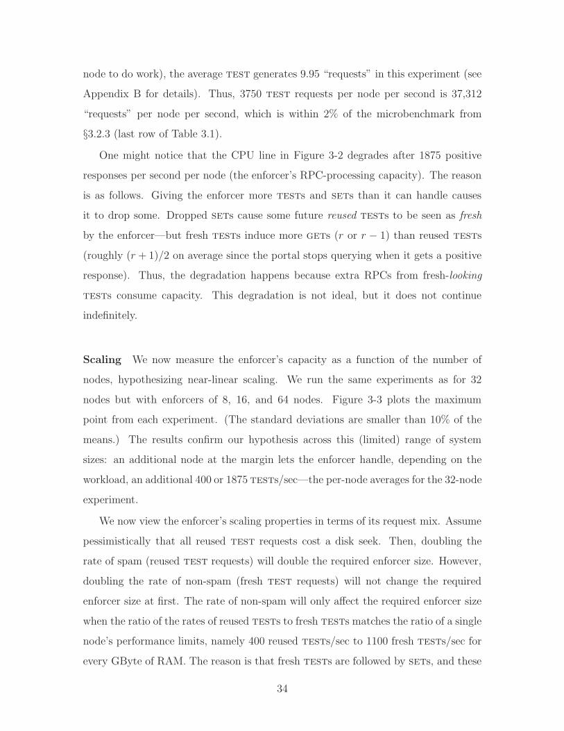
One might notice that the CPU line in Figure 3-2 degrades after 1875 positive

responses per second per node (the enforcer’s RPC-processing capacity). The reason

is as follows. Giving the enforcer more tests and sets than it can handle causes

it to drop some. Dropped sets cause some future reused tests to be seen as fresh

by the enforcer—but fresh tests induce more gets (r or r − 1) than reused tests

(roughly (r + 1)/2 on average since the portal stops querying when it gets a positive

response). Thus, the degradation happens because extra RPCs from fresh-looking

tests consume capacity. This degradation is not ideal, but it does not continue

indefinitely.

Scaling We now measure the enforcer’s capacity as a function of the number of

nodes, hypothesizing near-linear scaling. We run the same experiments as for 32

nodes but with enforcers of 8, 16, and 64 nodes. Figure 3-3 plots the maximum

point from each experiment. (The standard deviations are smaller than 10% of the

means.) The results confirm our hypothesis across this (limited) range of system

sizes: an additional node at the margin lets the enforcer handle, depending on the

workload, an additional 400 or 1875 tests/sec—the per-node averages for the 32-node

experiment.

We now view the enforcer’s scaling properties in terms of its request mix. Assume

pessimistically that all reused test requests cost a disk seek. Then, doubling the

rate of spam (reused test requests) will double the required enforcer size. However,

doubling the rate of non-spam (fresh test requests) will not change the required

enforcer size at first. The rate of non-spam will only affect the required enforcer size

when the ratio of the rates of reused tests to fresh tests matches the ratio of a single

node’s performance limits, namely 400 reused tests/sec to 1100 fresh tests/sec for

every GByte of RAM. The reason is that fresh tests are followed by sets, and these

34

0

500

1000

1500

2000

2500

3000

3500

0 50 100 150 200 250 300 0

20

40

60

80

100

120

Posi

tive

TE

ST r

espo

nses

(pkt

s/se

c/no

de)

(100

0s p

kts/

sec)

Sent "fresh"+"reused" TESTs(1000s pkts/sec)

CPU workloaddisk workload

Figure 3-2: For a 32-node enforcer, mean response rate to test requests as functionof sent test rate for disk- and CPU-bound workloads. The two y-axes show theresponse rate in different units: (1) per-node and (2) over the enforcer in aggregate.Here, r = 5, and each reported sample’s standard deviation is less than 9% of itsmean.

sets are a bottleneck only if nodes see more than 1100 puts per second per GByte

of RAM; see Table 3.1.

3.2.5 Estimating the Enforcer Size

We now give a rough estimate of the number of dedicated enforcer nodes required to

handle current e-mail volumes. The calculation is summarized in Table 3.2. Some

current estimates suggest 84 billion e-mail messages per day [31] and a spam rate

100 billion e-mails daily (target from §1.1)65% spam [42, 9]

65 billion disk seeks / day (pessimistic)400 disk seeks/second/node (§3.2.3)

86400 seconds/day

1881 nodes (from three quantities above)

Table 3.2: Estimate of enforcer size (based on average rates).

35

0

20

40

60

80

100

120

64 32 16 8Max

. Pos

itive

TE

ST r

espo

nses

(100

0s p

kts/

sec)

Number of nodes

CPU workloaddisk workload

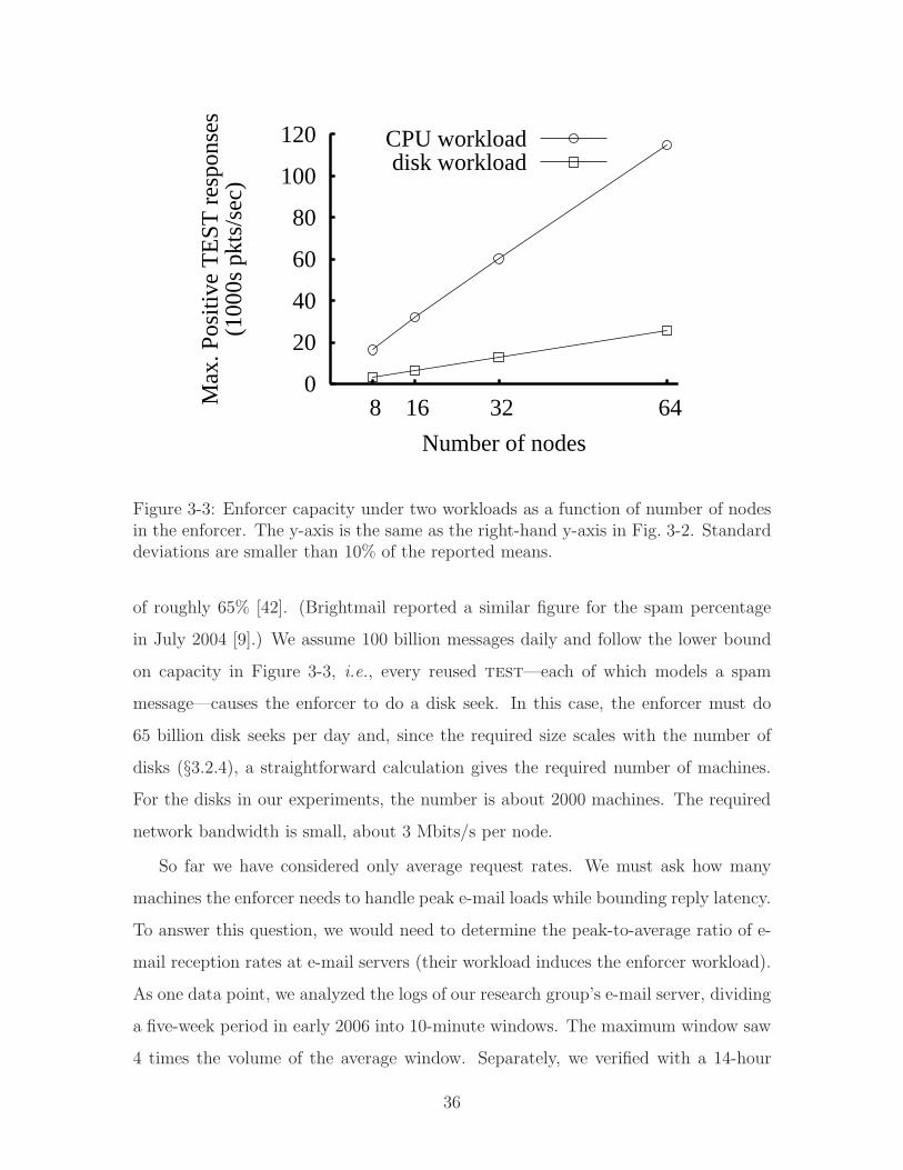
Figure 3-3: Enforcer capacity under two workloads as a function of number of nodesin the enforcer. The y-axis is the same as the right-hand y-axis in Fig. 3-2. Standarddeviations are smaller than 10% of the reported means.

of roughly 65% [42]. (Brightmail reported a similar figure for the spam percentage

in July 2004 [9].) We assume 100 billion messages daily and follow the lower bound

on capacity in Figure 3-3, i.e., every reused test—each of which models a spam

message—causes the enforcer to do a disk seek. In this case, the enforcer must do

65 billion disk seeks per day and, since the required size scales with the number of

disks (§3.2.4), a straightforward calculation gives the required number of machines.

For the disks in our experiments, the number is about 2000 machines. The required

network bandwidth is small, about 3 Mbits/s per node.

So far we have considered only average request rates. We must ask how many

machines the enforcer needs to handle peak e-mail loads while bounding reply latency.

To answer this question, we would need to determine the peak-to-average ratio of e-

mail reception rates at e-mail servers (their workload induces the enforcer workload).

As one data point, we analyzed the logs of our research group’s e-mail server, dividing

a five-week period in early 2006 into 10-minute windows. The maximum window saw

4 times the volume of the average window. Separately, we verified with a 14-hour

36

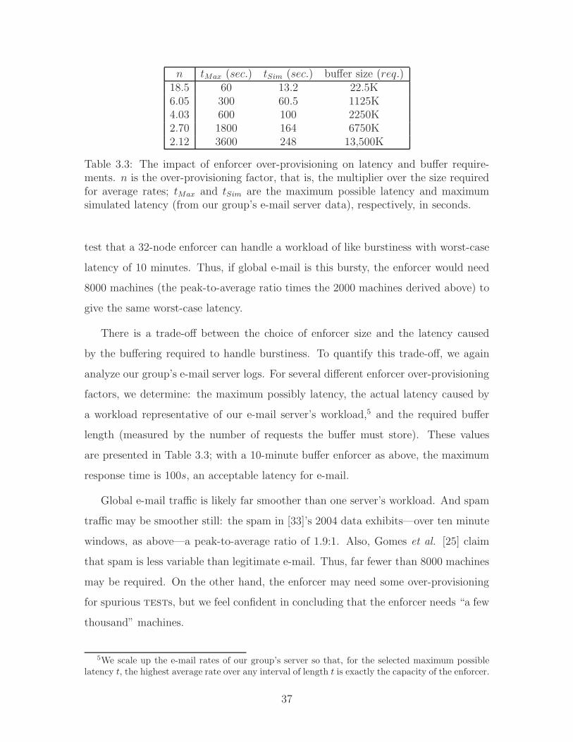
n tMax (sec.) tSim (sec.) buffer size (req.)18.5 60 13.2 22.5K6.05 300 60.5 1125K4.03 600 100 2250K2.70 1800 164 6750K2.12 3600 248 13,500K

Table 3.3: The impact of enforcer over-provisioning on latency and buffer require-ments. n is the over-provisioning factor, that is, the multiplier over the size requiredfor average rates; tMax and tSim are the maximum possible latency and maximumsimulated latency (from our group’s e-mail server data), respectively, in seconds.

test that a 32-node enforcer can handle a workload of like burstiness with worst-case

latency of 10 minutes. Thus, if global e-mail is this bursty, the enforcer would need

8000 machines (the peak-to-average ratio times the 2000 machines derived above) to

give the same worst-case latency.

There is a trade-off between the choice of enforcer size and the latency caused

by the buffering required to handle burstiness. To quantify this trade-off, we again

analyze our group’s e-mail server logs. For several different enforcer over-provisioning

factors, we determine: the maximum possibly latency, the actual latency caused by

a workload representative of our e-mail server’s workload,5 and the required buffer

length (measured by the number of requests the buffer must store). These values

are presented in Table 3.3; with a 10-minute buffer enforcer as above, the maximum

response time is 100s, an acceptable latency for e-mail.

Global e-mail traffic is likely far smoother than one server’s workload. And spam

traffic may be smoother still: the spam in [33]’s 2004 data exhibits—over ten minute

windows, as above—a peak-to-average ratio of 1.9:1. Also, Gomes et al. [25] claim

that spam is less variable than legitimate e-mail. Thus, far fewer than 8000 machines

may be required. On the other hand, the enforcer may need some over-provisioning

for spurious tests, but we feel confident in concluding that the enforcer needs “a few

thousand” machines.

5We scale up the e-mail rates of our group’s server so that, for the selected maximum possiblelatency t, the highest average rate over any interval of length t is exactly the capacity of the enforcer.

37

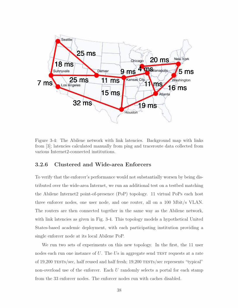
Figure 3-4: The Abilene network with link latencies. Background map with linksfrom [3]; latencies calculated manually from ping and traceroute data collected fromvarious Internet2-connected institutions.

3.2.6 Clustered and Wide-area Enforcers

To verify that the enforcer’s performance would not substantially worsen by being dis-

tributed over the wide-area Internet, we run an additional test on a testbed matching

the Abilene Internet2 point-of-presence (PoP) topology. 11 virtual PoPs each host

three enforcer nodes, one user node, and one router, all on a 100 Mbit/s VLAN.

The routers are then connected together in the same way as the Abilene network,

with link latencies as given in Fig. 3-4. This topology models a hypothetical United

States-based academic deployment, with each participating institution providing a

single enforcer node at its local Abilene PoP.

We run two sets of experiments on this new topology. In the first, the 11 user

nodes each run one instance of U . The Us in aggregate send test requests at a rate

of 19,200 tests/sec, half reused and half fresh; 19,200 tests/sec represents “typical”

non-overload use of the enforcer. Each U randomly selects a portal for each stamp

from the 33 enforcer nodes. The enforcer nodes run with caches disabled.

38

As expected, spreading the enforcer’s nodes across a topology that introduces

per-link latency increases the enforcer’s response time. For the Abilene topology, the

average time for the enforcer to respond to a client is 372 ms (σ = 164 ms), compared

to 51.8 ms (σ = 122 ms) for a monolithic enforcer.

In the second set of experiments on the Abilene topology, the Us generate request

rates from 50,000 to 150,000 fresh and reused tests/sec in aggregate, and the enforcer

nodes run with caches large enough to hold all set stamps. As expected, the new

topology does not degrade the enforcer’s aggregate CPU-bound throughput, which is

the expected 33 · 3750 = 123, 750 fresh and reused tests/sec.

Finally, we also examine the extent to which using DCCP instead of UDP for

internal RPCs impacts performance; a microbenchmark experiment with a 2-node

enforcer suggests that DCCP may reduce RPC processing capacity by up to 30%,

however, DCCP does not impact the enforcer’s disk and memory bottlenecks, and

thus our estimate of the required enforcer size remains unchanged.

3.2.7 Avoiding “Distributed Livelock”

We now briefly evaluate the scheme to avoid livelock (from §2.2.3). The goal of

the scheme is to maximize correct test responses under high load. To verify that

the scheme meets this goal, we run the following experiment: 20 U instances send

test requests (half fresh, half reused) at high rates, first, to a 32-node enforcer with

the scheme and then, for comparison, to an otherwise identical enforcer without the

scheme. Here, r = 5 and the nodes’ caches are enabled. Also, each stamp is used

no more than twice; tests thus generate multiple gets, some of which are dropped

by the enforcer without the scheme. Figure 3-5 graphs the positive responses as a

function of the sent test rate. At high sent test rates, an enforcer with the scheme

gives twice as many positive responses—that is, blocks more than twice as much

spam—as an enforcer without the scheme.

39

10

20

30

40

50

60

70

0 50 100 150 200 250 300 350

Posi

tive

TE

ST r

espo

nses

(100

0s p

kts/

sec)

Sent TEST rate (1000s pkts/sec)

with schemewithout scheme

Figure 3-5: Effect of livelock avoidance scheme from §2.2.3. As the sent test rateincreases, the ability of an enforcer without the scheme to respond accurately toreused tests degrades.

3.2.8 Limitations

Although we have tested the enforcer under heavy load to verify that it does not

degrade, we have not tested a flash crowd in which a single stamp s is geted by

all (several thousand) of the enforcer nodes. Note, however, that handling several

thousand simultaneous gets is not difficult because after a single disk seek for s, an

assigned node has the needed key-value pair in its cache.

We have also not addressed heterogeneity. For static heterogeneity, i.e., nodes that

have unequal resources (e.g., CPU, RAM), the bunker can adjust the load-balanced

assignment of keys to values. Dynamic heterogeneity, i.e., when certain nodes are

busy, will be handled by the enforcer’s robustness to unresponsive nodes and by the

application’s insensitivity to latency.

40

Chapter 4

Trade-offs in “Distributed Livelock

Avoidance”

In this chapter, we consider several different prioritization schemes for “livelock avoid-

ance.” Recall that the scheme presented in §2.2.3 considered test and set requests

to form a single class; here, we consider prioritization schemes in which test or set

has a higher priority than the other.

Throughout this chapter, our goal is to maximize the rate of blocked spam; we do

not concern ourselves with latency or even “not found” responses to tests, as the

current implementation treats a “not found” response in the same way as no response

at all.

We focus our attention on the external RPCs, test and set, and assume that

any generated internal RPCs and their responses will be admitted. We consider three

possible prioritization schemes based on packet type and one based on packet content.

To evaluate the different schemes, we consider two overload conditions. In the first,

every reused stamp is the same stamp, which nodes (unrealistically) do not cache. In

the second, each “reused” stamp is used exactly twice.

For the rest of this chapter, we let L (for “load”) be the sent test rate, a fraction s

of which is for reused stamps. R is the enforcer’s RPC capacity, and r is its replication

factor. For simplicity, we assume that r is small compared to the enforcer’s size, and

we ignore the probability that tests and sets occur at assigned nodes.

41

4.1 Repeated Use of a Single Stamp

In this section, we consider an overload scenario in which all reused tests are for the

same stamp, and that this stamp is already stored on at least 1 assigned node.

Recall from §2.2 that an admitted fresh test generates r gets and r get re-

sponses, and that a reused test generates r+12

gets and r+12

get responses in ex-

pectation; a fresh test further induces 1 set, 1 put, and 1 put response. (See

Appendix A for a detailed analysis.)

Thus, an admitted fresh test will generate a total of 1 + r + r = 2r + 1 RPCs,

and, if the subsequent set is admitted, 3 additional RPCs, including the test itself.

An admitted reused test will generate a total of 1 + r+12

+ r+12

= r + 2 RPCs, and

will never induce a set.

4.1.1 test = set

We first consider the prioritization scheme in which tests and sets are served in

a round-robin manner by the enforcer, as described in §2.2.3. To determine how

the fraction of blocked spam is affected by overload, we first calculate the enforcer’s

capacity and then analyze what happens as the test rate is increased.

At capacity, every sent test and set is admitted (note that our assumption that

all gets and put successfully complete guarantees that any admitted test or set

will be successfully completed). The enforcer’s capacity is thus given by the invariant

R = L(1− s)(2r + 1 + 3)︸ ︷︷ ︸

fresh

+ Ls(r + 2)︸ ︷︷ ︸

reused

.

To determine the capacity (rate of blocked spam), we must find Ls:

Ls =Rs

(1− s)(2r + 4) + s(r + 2).

As we increase L past this limit, the enforcer will begin to drop fresh tests, reused

tests, and sets, all at the same rate; let Q be the fraction of tests and sets that

42

are admitted. Note, however, that the number of generated sets does not increase

with L but instead with the rate of admitted tests. Thus if Q ·L(1− s) fresh tests

are admitted, we expect Q2 · L(1 − s) sets to be admitted, as each generated set

is admitted with probability Q. The exact relationship between Q and L can be

determined, but for now we note that Q approximately decreases with 1/L. In the

limit as Q approaches 0, the number of admitted sets approaches 0, and thus the

number of admitted reused tests approaches Rs(1−s)(2r+1)+s(r+2)

.

4.1.2 test ≺ set

We next consider a scheme in which tests precede sets, that is, a scheme that

prioritizes tests over sets. As before, capacity is given by Ls = Rs(1−s)(2r+4)+s(r+2)

.

However, under this scheme, increasing the rate of sent tests now causes tests to

be selected over sets. Under our stamp reuse assumptions (one stamp reused many

times; that stamp is already set), sets are irrelevant. Thus, the maximum test

capacity is when sets are dropped and Ls = Rs(1−s)(2r+1)+s(r+2)

, the same as in the

test = set case.

4.1.3 test ≻ set

Now we consider a scheme that prioritizes sets over tests. Capacity is again given

by Ls = Rs(1−s)(2r+4)+s(r+2)

, but now increasing the test rate will cause the enforcer

to drop fresh and reused tests but not sets, and thus the number of admitted

tests and sets does not change. In the limit as L → ∞, then, capacity remains

Rs(1−s)(2r+4)+s(r+2)

.

To maximize capacity in the case when all reused tests request the same stamp,

thus, the enforcer should prioritize tests over sets; at a high level this is true because

sets do not improve the enforcer’s ability to respond to reused tests. However,

if sets are necessary—we consider this case below—prioritizing tests may prove

disastrous.

43

4.2 Stamps Used At Most Twice

If stamps are each used at most twice—as we assume in most of Chapter 3—ensuring

that the enforcer admits sets becomes much more important. As before, an admitted

fresh test generates r gets and r get responses, and 1 set, which itself generates

a put and a put response. An admitted reused test, however, is not so simple. Let

Qt, Qs be the fraction of tests, sets that the enforcer admits. Then, a reused test’s

stamp will have been previously stored with probability Qt ·Qs, as with probability Qt

the first test was admitted, and with probability Qs, the set was admitted. Thus,

a reused test generates r+12

gets and get responses with probability Qt ·Qs. With

probability 1−Qt ·Qs, a reused test generates r gets and get responses, and then

further generates a set. Since sets are admitted with probability Qs, our invariant

is:

R = Qt ·L(1−s)(1+2r +Qs ·3)+Qt ·Ls [1 + QtQs(r + 1) + (1−QtQs)(2r + Qs · 3)]

(4.1)

Given this invariant, the rate at which the enforcer blocks spam is LsQt ·QtQs.

4.2.1 test = set

Now consider again the prioritization scheme in which tests and sets are served

in a round-robin manner. Under this scheme, Qs = Qt, which for simplicity we

now call Q. Solving equation 4.1 for Q = Qs = Qt is non-trivial, but fortunately

unnecessary. Observe that when Q is small, which intuitively must occur when L is

large, Q ∝ 1L. Thus the amount of blocked spam is LsQ3 ∝ s

L2 , and in the limit

L→∞, sL2 approaches 0.

4.2.2 test ≺ set

If tests are preferred over sets, the behavior when L approaches infinity can be

intuitively determined: no sets will be admitted, and as a consequence no spam will

be blocked.

44

4.2.3 test ≻ set

If sets are preferred over tests, however, the behavior is more complex. We can

first simplify by noting that Qs = 1. Under legitimate use, a client will only generate

a set after receiving a response to a test, and thus for any sets to be generated,

some tests must be admitted, which can only occur if all sets are admitted. The

total quantity of spam blocked is LsQt · Qt, the number of admitted reused tests

times the probability that the original test for a reused test’s queried stamp was

admitted. Beginning with equation 4.1, we derive:

R = Qt · L(1− s)(1 + 2r + 3) + Qt · Ls [1 + Qt(r + 1) + (1−Qt)(2r + 3)]

0 = R−QtL [(1 + 2r + 3)] + Q2t Ls [r + 2]

Qt =L(1 + 2r + 3)±

√

L2(1 + 2r + 3)2 − 4(R)Ls(r + 2)

2Ls(r + 2)

Qt =(1 + 2r + 3)±

√

(1 + 2r + 3)2 − 1L4(R)s(r + 2)

2s(r + 2)

Once again, as L→∞, Qt → 0, and limL→∞LsQt ·Qt = 0.

This result is also intuitive: the probability that a single stamp’s fresh and reused

tests both succeed approaches 0 as the fraction of tests that are admitted ap-

proaches 0. Note, however, that under slight overload, as when L is not much greater

than capacity, the amount of blocked spam is greater than in the test = set case;

see Figure 4-1.

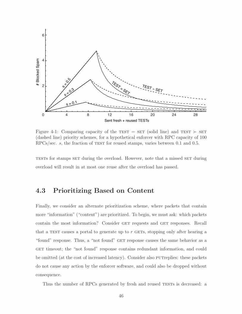
What conclusions can we draw from these results? First, we see that if the

stamps being test during overload are also those being set—as in a chronic over-

load condition—the ability of the enforcer to block spam suffers dramatically, but that

preferring sets over tests helps the enforcer block spam if the overload is not too

great. However, if the overload concerns stamps that have been set before overload

began—as in §4.1 above—preferring tests over sets yields a small improvement.

Note that the analysis presented here only considers how the enforcer performs

during overload, and not the effects of the chosen priority scheme after the overload

has passed; sets are a more important consideration if we concern ourselves with

45

0 4 8 12 16 20 24 28

2

4

6

Sent fresh + reused TESTs

# B

locked S

pam

s =

0.5

s = 0.1

s = 0

.3TEST ≻ SET

TEST = SET

Figure 4-1: Comparing capacity of the test = set (solid line) and test ≻ set

(dashed line) priority schemes, for a hypothetical enforcer with RPC capacity of 100RPCs/sec. s, the fraction of test for reused stamps, varies between 0.1 and 0.5.

tests for stamps set during the overload. However, note that a missed set during

overload will result in at most one reuse after the overload has passed.

4.3 Prioritizing Based on Content

Finally, we consider an alternate prioritization scheme, where packets that contain

more “information” (“content”) are prioritized. To begin, we must ask: which packets

contain the most information? Consider get requests and get responses. Recall

that a test causes a portal to generate up to r gets, stopping only after hearing a

“found” response. Thus, a “not found” get response causes the same behavior as a

get timeout; the “not found” response contains redundant information, and could

be omitted (at the cost of increased latency). Consider also putreplies: these packets

do not cause any action by the enforcer software, and could also be dropped without

consequence.

Thus the number of RPCs generated by fresh and reused tests is decreased: a

46

fresh test now generates 1(test)+ r(get)+ 1(set)+ 1(put) = 3+ r RPCs instead

of 1(test) + 2r(get, resp.) + 1(set) + 2(put, resp.) = 4 + 2r RPCs. Similarly, a

reused test now generates 1 + r+12

+ 1 = 2 + r+12

RPCs instead of (r + 2) RPCs.

These savings mean that the capacity of the enforcer under overload is increased from

Ls = Rs(1−s)(2r+4)+s(r+2)

to

Ls =Rs

(1− s)(r + 3) + s( r+12

+ 2).

For r = 5, s = 0.5, the conditions used in most of §3.2, this corresponds to an

increase in RPC capacity of 62%.

The analysis from the packet type-based prioritization schemes still applies on top

of content-based prioritization, which can be thought of as simply a mechanism for

decreasing the number of RPCs generated by tests and sets.

47

48

Chapter 5

Related Work

As the number of proposed spam control measures approaches ∞, placing one’s own

approach in context becomes more and more difficult. My focus in this thesis has

been on the distributed system facet of DQE; for completeness, I excerpt the spam

control section of [59]’s related work, and then focus on related distributed systems

and analyses.

5.1 Spam Control

Spam filters (e.g., [54, 28]) analyze incoming e-mail to classify it as spam

or legitimate. While these tools certainly offer inboxes much relief, they

do not achieve our top-level goal of reliable e-mail (see §1). Moreover,

filters and spammers are in an arms race that makes classification ever

harder.

The recently-proposed Re: [24] shares our reliable e-mail goal. Re: uses

friend-of-friend relationships to let correspondents whitelist each other

automatically. In contrast to DQE, Re: allows some false positives (for

non-whitelisted senders), but on the other hand does not require globally

trusted entities (like the quota allocators and bunker, in our case). Tem-

pleton [57] proposes an infrastructure formed by cooperating ISPs to han-

dle worldwide e-mail; the infrastructure throttles e-mail from untrusted

49

sources that send too much. Like DQE, this proposal tries to control vol-

umes but unlike DQE presumes the enforcement infrastructure is trusted.

Other approaches include single-purpose addresses [32] and techniques by

which e-mail service providers can stop outbound spam [27].

In postage proposals (e.g., [23, 49]), senders pay receivers for each e-

mail; well-behaved receivers will not collect if the e-mail is legitimate.

This class of proposals is critiqued by Levine [37] and Abadi et al. [1].

Levine argues that creating a micropayment infrastructure to handle the

world’s e-mail is infeasible and that potential cheating is fatal. Abadi et al.

argue that micropayments raise difficult issues because “protection against

double spending [means] making currency vendor-specific .... There are

numerous other issues ... when considering the use of a straight micro-

commerce system. For example, sending email from your email account

at your employer to your personal account at home would in effect steal

money from your employer” [1].

With pairwise postage, receivers charge CPU cycles [20, 10, 5] or mem-

ory cycles [2, 19] (the latter being fairer because memory bandwidths are

more uniform than CPU bandwidths) by asking senders to exhibit the

solution of an appropriate puzzle. Similarly, receivers can demand human

attention (e.g., [55]) from a sender before reading an e-mail.

Abadi et al. pioneered bankable postage [1]. Senders get tickets from

a “Ticket Server” (TS) (perhaps by paying in memory cycles) and attach

them to e-mails. Receivers check tickets for freshness, cancel them with

the TS, and optionally refund them. Abadi et al. note that, compared

to pairwise schemes, this approach offers: asynchrony (senders get tickets

“off-line” without disrupting their workflow), stockpiling (senders can get

tickets from various sources, e.g., their ISPs), and refunds (which conserve

tickets when the receiver is friendly, giving a higher effective price to

spammers, whose receivers would not refund).

DQE is a bankable postage scheme, but TS differs from DQE in three

50

ways: first, it does not separate allocation and enforcement (see §1);

second, it relies on a trusted central server; and third, it does not pre-

serve sender-receiver e-mail privacy. Another bankable postage scheme,

SHRED [36], also has a central, trusted cancellation authority. Unlike

TS and SHRED, DQE does not allow refunds (letting it do so is future

work for us), though receivers can abstain from canceling stamps of known

correspondents. . . .

Goodmail [26]—now used by two major e-mail providers [16]—resembles

TS. (See also Bonded Sender [8], which is not a postage proposal but has

the same goal as Goodmail.) Goodmail accredits bulk mailers, trying to

ensure that they send only solicited e-mail, and tags their e-mail as “cer-

tified”. The providers then bypass filters to deliver such e-mail to their

customers directly. However, Goodmail does not eliminate false positives

because only “reputable bulk mailers” get this favored treatment. More-

over, like TS, Goodmail combines allocation and enforcement and does

not preserve privacy.

5.2 Related Distributed Systems1

As a distributed storage service, the enforcer shares many properties with DHTs and

other distributed storage systems. Indeed, an early design used a DHT in the enforcer,

but we discovered that a DHT’s goals do not perfectly match the enforcer’s [6]. Many

DHTs (see, e.g., [56, 51, 63, 48]) are designed for large systems with decentralized

management of membership and of peer arrivals and departures; in contrast, the

enforcer is small and is assumed to have low churn. As a result, the enforcer can

have static membership (provided by the bunker), allowing for mutually untrusting

nodes that can focus on handling requests instead of routing them. This is not to

say that all DHTs must have mutually trusting nodes; for example, Castro et al. [11]

propose a mechanism for handling nodes that route for each other and are mutually

1This section is modeled on §4.3 and §7 of [59].

51

untrusting, but with high complexity. Further, one-hop DHTs [29, 30] do away with

routing altogether, but membership information must still be propagated in a trusted

manner.

Static configuration is common in the replicated state machine literature; see,

e.g., [12, 52]. The BAR model [4] and Rosebud [50] both assume (as DQE does) that

configuration is conducted by a trusted party. Byzantine quorum solutions also make

use of static configuration; see, e.g., [39, 40]. The enforcer differs from these systems

by tolerating faults without mechanism beyond the bunker. Enforcer nodes do not

keep track of which other nodes are up, nor do nodes or clients attempt to protect

data; fault-tolerance is possible because of our application’s insensitivity to lost data.

Additionally, while many of these systems use TCP connections between nodes

in the wide-area, a few propose new protocols for inter-node communication. For

example, DHash++ [17] uses an alternative non-TCP congestion control protocol, the

Striped Transport Protocol (STP). STP is designed to take advantage of DHash++’s

distribution of data segments among nodes; nodes send requests to many peers and

receive their responses simultaneously, reducing latency. Unlike TCP’s per-connection

state, each node using STP maintains a single window for outstanding requests, under

the assumption that congestion will occur on or near an edge link. However, STP

provides semantics not useful to DQE: enforcer nodes issue requests serially, and

(unlike DHash++) data from just a single node suffices to respond to the client.

There is also work related to the livelock avoidance scheme from §2.2.3 and Chap-

ter 4. First, there is a lot of work that addresses overload conditions in general;

much of this work uses fine-grained resource allocation to prevent servers from being

overloaded (see SEDA [62, 61], LRP [18], and Defensive Programming [46] and their

bibliographies). Additional work focuses on clusters of identical servers and how to

balance load among them (see Neptune [53] and its bibliography). However, all of

this research focuses on management of single hosts; the livelock avoidance scheme we

propose concerns single requests that require the resources of many separate hosts.

52

5.3 Related Measurement Work

There is both academic and anecdotal work dealing with spam and e-mail volumes

and trends. Gomes et al. [25] analyze size and time distribution in both spam and

legitimate e-mail at Federal University of Minas Gerais in Brazil; as mentioned in

§3.2.5, they claim that spam arrival rates have a peak-to-average ratio of 2.3 using

1-hour granularity (compared to 5.4 for non-spam). They also compare spam and

non-spam message sizes and recipient counts, and find that spam is once again less

variable than non-spam. Jung and Sit [33] analyze spam trends in the context of DNS

blacklists, finding that the distribution of SMTP connections from spam-sending hosts

has become more heavy-tailed in that time (suggesting that blacklists may become

less effective); they generously provided their data for us to use in determining peak-

to-average rates in spam data entering MIT’s networks.

Work on e-mail use includes: Bertolotti and Calzarossa [7] analyze interarrival

time and message size distributions for e-mail, and additionally consider e-mail server

use by local POP and IMAP clients; they find that no one distribution well-models

e-mail interarrival times, but that the tail is best modeled by a Pareto distribution,

while the body is best modeled by a Weibull distribution. Pang et al. [43] analyze

e-mail use in the context of all traffic in a medium-sized organization, and find that

most WAN SMTP connections last around 1.5-6 seconds and transfer under 1 MByte

of data. Many studies (see, e.g., [7, 58]) also discuss the correlation between spam

and the number of messages sent per SMTP connection.

Anecdotal studies of the costs of spam include those discussed in the introduction

([15, 14]), claiming that false positives will cost U.S. businesses about $419 million

in 2008. As a testament to the variability of estimation, however, another study

([22]) claims that blocked legitimate e-mail cost U.S. businesses $3.5 billion in 2003;

anecdotal spam volume studies include [9, 47, 42], claiming anywhere from 60 billion

to 140 billion messages sent in 2004.

Finally, there is also related work on measurement and simulation. Paxson and

Floyd [44] suggest that incoming connection arrivals can be well-modeled by Poisson

53

processes (even though packet arrivals more generally cannot be); in fact, the software

we use to test the enforcer generates requests by a Poisson process. The QoS literature

contains studies of peak-to-average traffic rates in the context of their impact on total

delay: for example, Clark et al. [13] claim that buffering helps reduce provisioning

when the workload size is not heavy-tailed, as is the case in our application.2

2E-mail use (e.g., volume in bytes) may be heavy-tailed, but the test and set requests of theenforcer are of constant size.

54

Chapter 6

Conclusions

Our aim is to show that the technical problems surrounding an e-mail quota system

are solvable. To this end, we present the design, implementation, and evaluation of

DQE, a quota system with enforcer that has the properties we initially set out in

Chapter 1: scalability, resilience to faults and attacks, high-throughput, and mutual

distrust between nodes.

In this work, we show that an enforcer composed of just a few thousand dedi-

cated, mutually untrusting nodes can handle stamp queries at the rate generated by

the volume of the world’s e-mail. The enforcer’s simplicity—nodes do not maintain

neighbor state, manage replicas, or even trust each other—helps convince us of its

practicality.

My main focus in this thesis has been on the evaluation of DQE, with three main

results. First, the enforcer is high-performance: running our software, a single node

is capable of handling over 38,000 RPCs/sec. Second, the enforcer scales well with

size: all else being equal, an enforcer with twice as many nodes will handle twice as

many requests. Third, the enforcer is resistant to faults: with up to 20% of its nodes

“bad”, the enforcer is still able to limit stamp use to 1.5 uses/stamp on average.

I separately present an analysis of different prioritizations for our livelock avoid-

ance scheme, and show that—regardless of priority—the scheme is effective at han-

dling transient overload: chronic overload severely degrades the enforcer’s ability to

block spam.

55

Future work for our team includes further analysis of “distributed livelock avoid-

ance”, including the development of a library to be used by future distributed system

engineers in helping their designs handle transient overload.

56

Appendix A

Relating Microbenchmarks to

System Performance

In this appendix,1 we calculate how many RPCs are induced by a test in expectation.

Claim 1 The average number of RPCs per test in the 32-node enforcer experiments

described in §3.2.4, in which 50% of test requests are “fresh”, is 9.95.

Proof:

Recall from §3.2.4 that the 32-node enforcer is configured with replication factor

r = 5. On receiving a fresh test, the portal must contact all 5 assigned nodes for the

stamp. With probability 5/32, the portal is an assigned node for the stamp, and one

of the gets will be local. Thus, we expect a fresh test to generate 532·4+ 27

32·5 = 4.84

get requests and get responses. (Note that a request and a response both cause the

CPU to do roughly the same amount of work, and thus an RPC response counts as

an RPC in our calculations.) A fresh test will also be followed by a set that will

in turn cause both a put and a put response with probability 31/32 = 0.97. (With

probability 1/32, the portal is one of the assigned nodes and chooses itself as the node

to put to, generating no remote put.)

A reused test generates no subsequent set, put request, or put response. In

addition, for reused tests, the number of induced gets is less than in the fresh

1The contents of this appendix appear in [60].

57

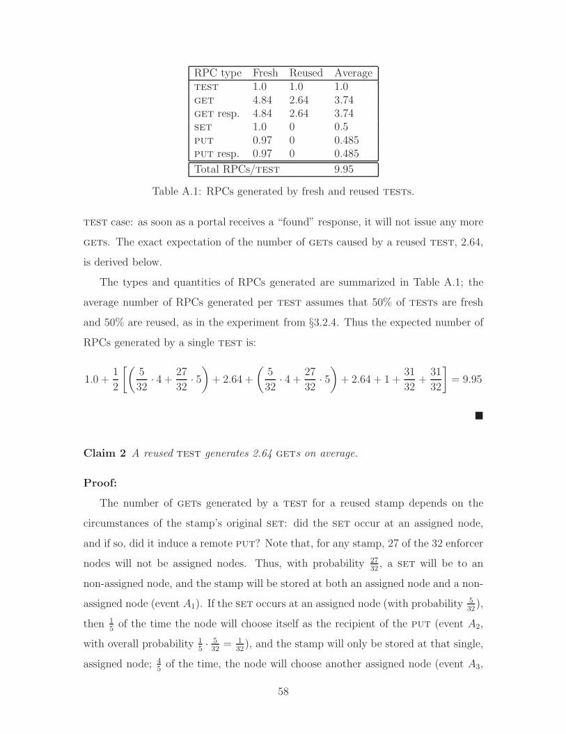
RPC type Fresh Reused Averagetest 1.0 1.0 1.0get 4.84 2.64 3.74get resp. 4.84 2.64 3.74set 1.0 0 0.5put 0.97 0 0.485put resp. 0.97 0 0.485

Total RPCs/test 9.95

Table A.1: RPCs generated by fresh and reused tests.

test case: as soon as a portal receives a “found” response, it will not issue any more

gets. The exact expectation of the number of gets caused by a reused test, 2.64,

is derived below.

The types and quantities of RPCs generated are summarized in Table A.1; the

average number of RPCs generated per test assumes that 50% of tests are fresh

and 50% are reused, as in the experiment from §3.2.4. Thus the expected number of

RPCs generated by a single test is:

1.0 +1

2

[(5

32· 4 +

27

32· 5

)

+ 2.64 +

(5

32· 4 +

27

32· 5

)

+ 2.64 + 1 +31

32+

31

32

]

= 9.95

�

Claim 2 A reused test generates 2.64 gets on average.

Proof:

The number of gets generated by a test for a reused stamp depends on the

circumstances of the stamp’s original set: did the set occur at an assigned node,

and if so, did it induce a remote put? Note that, for any stamp, 27 of the 32 enforcer

nodes will not be assigned nodes. Thus, with probability 2732

, a set will be to an

non-assigned node, and the stamp will be stored at both an assigned node and a non-

assigned node (event A1). If the set occurs at an assigned node (with probability 532

),

then 15

of the time the node will choose itself as the recipient of the put (event A2,

with overall probability 15· 5

32= 1

32), and the stamp will only be stored at that single,

assigned node; 45

of the time, the node will choose another assigned node (event A3,

58

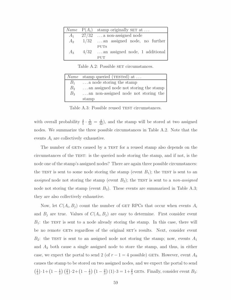
Name P(Ai) stamp originally set at . . .A1 27/32 . . . a non-assigned nodeA2 1/32 . . . an assigned node, no further

putsA3 4/32 . . . an assigned node, 1 additional

put

Table A.2: Possible set circumstances.

Name stamp queried (tested) at . . .B1 . . . a node storing the stampB2 . . . an assigned node not storing the stampB3 . . . an non-assigned node not storing the

stamp

Table A.3: Possible reused test circumstances.

with overall probability 45· 5

32= 4

32), and the stamp will be stored at two assigned

nodes. We summarize the three possible circumstances in Table A.2. Note that the

events Ai are collectively exhaustive.

The number of gets caused by a test for a reused stamp also depends on the

circumstances of the test: is the queried node storing the stamp, and if not, is the

node one of the stamp’s assigned nodes? There are again three possible circumstances:

the test is sent to some node storing the stamp (event B1); the test is sent to an

assigned node not storing the stamp (event B2); the test is sent to a non-assigned

node not storing the stamp (event B3). These events are summarized in Table A.3;

they are also collectively exhaustive.

Now, let C(Ai, Bj) count the number of get RPCs that occur when events Ai

and Bj are true. Values of C(Ai, Bj) are easy to determine. First consider event

B1: the test is sent to a node already storing the stamp. In this case, there will

be no remote gets regardless of the original set’s results. Next, consider event

B2: the test is sent to an assigned node not storing the stamp; now, events A1

and A2 both cause a single assigned node to store the stamp, and thus, in either

case, we expect the portal to send 2 (of r− 1 = 4 possible) gets. However, event A3

causes the stamp to be stored on two assigned nodes, and we expect the portal to send(

12

)·1+

(1− 1

2

) (23

)·2+

(1− 1

2

) (1− 2

3

)(1)·3 = 1+ 2

3gets. Finally, consider event B3:

59

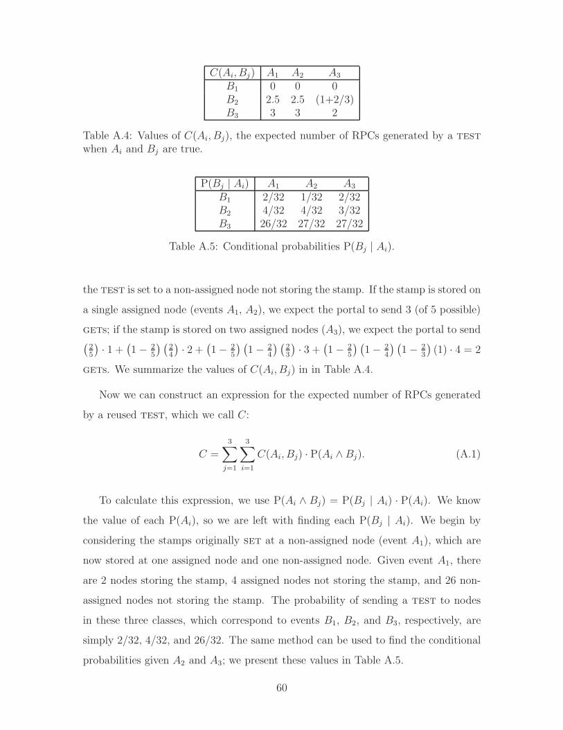
C(Ai, Bj) A1 A2 A3

B1 0 0 0B2 2.5 2.5 (1+2/3)B3 3 3 2

Table A.4: Values of C(Ai, Bj), the expected number of RPCs generated by a test

when Ai and Bj are true.

P(Bj | Ai) A1 A2 A3

B1 2/32 1/32 2/32B2 4/32 4/32 3/32B3 26/32 27/32 27/32

Table A.5: Conditional probabilities P(Bj | Ai).

the test is set to a non-assigned node not storing the stamp. If the stamp is stored on

a single assigned node (events A1, A2), we expect the portal to send 3 (of 5 possible)

gets; if the stamp is stored on two assigned nodes (A3), we expect the portal to send(

25

)· 1 +

(1− 2

5

) (24

)· 2 +

(1− 2

5

) (1− 2

4

) (23

)· 3 +

(1− 2

5

) (1− 2

4

) (1− 2

3

)(1) · 4 = 2

gets. We summarize the values of C(Ai, Bj) in in Table A.4.

Now we can construct an expression for the expected number of RPCs generated

by a reused test, which we call C:

C =3∑

j=1

3∑

i=1

C(Ai, Bj) · P(Ai ∧Bj). (A.1)

To calculate this expression, we use P(Ai ∧ Bj) = P(Bj | Ai) · P(Ai). We know

the value of each P(Ai), so we are left with finding each P(Bj | Ai). We begin by

considering the stamps originally set at a non-assigned node (event A1), which are

now stored at one assigned node and one non-assigned node. Given event A1, there

are 2 nodes storing the stamp, 4 assigned nodes not storing the stamp, and 26 non-

assigned nodes not storing the stamp. The probability of sending a test to nodes

in these three classes, which correspond to events B1, B2, and B3, respectively, are

simply 2/32, 4/32, and 26/32. The same method can be used to find the conditional

probabilities given A2 and A3; we present these values in Table A.5.

60

Combining the values of C(Ai, Bj) with the joint probabilities, we compute, from

equation (A.1), C = 2.64.

�

61

62

Appendix B

Exact Expectation Calculation in

“Crashed” Experiment

In this appendix,1 we derive an exact expression for expected stamp use in the

“crashed” experiment from §3.2.2. (The expression is stated in footnote 4.) Recall

from that section that n is the number of nodes in the system, p is the probability a

machine is “bad” (i.e., does not respond to queries), m = n(1− p) is the number of

“up” or “good” machines, stamps are queried 32 times, and r, the replication factor,

is 3.

Claim 3 The expected number of uses per stamp in the “crashed” experiment from §3.2.2

is:

(1− p)3(1) + 3p2(1− p)α + 3p(1− p)2β + p3m

(

1−

(m− 1

m

)32)

, for

α =m∑

i=1

i

(2

3

)i−11

m

(

1 +m− i

3

)

,

β =

m−1∑

i=1

i

(1

3

)i−1m− i

m(m− 1)

(

2 +2

3(m− (i + 1))

)

1The contents of this appendix appear in [60].

63

Proof:

To prove this claim, we consider 4 cases: 0 of a stamp’s 3 assigned nodes are good;

1 is good; 2 are good; all 3 are good.

Let U(s) be the number of times a stamp s is used. We calculate the expected

value of U(s) in each of the four cases. The first case is trivial: if all of s’s assigned

nodes are good (which occurs with probability (1−p)3), the stamp will be used exactly

once.

Next, to determine E[U ] for stamp with no good assigned nodes (probability p3),

we recall the facts of the experiment: stamps are queried 32 times at random portals,

and once a stamp has been set at a portal, no more reuses of the stamp will occur

at that portal. Thus, the expected number of times that s will be used, if none of

its assigned nodes is good, is the expected number of distinct bins (out of m) that

32 random balls will cover. Since the probability a bin isn’t covered is(

m−1m

)32, the

expected value of U(s) in this case is:

m

(

1−

(m− 1

m

)32)

.

We now compute the expected number of stamp uses for stamps with one or two

good assigned nodes. In either case:

E[U ] = 1 · P (exactly 1 use) + 2 · P (exactly 2 uses) + · · ·

For stamps with one good assigned node (probability (1−p)p2) there are two ways

for the stamp to be used exactly once: either, with probability 1m

, the stamp is test

and then set at the one good assigned node, or, with probability(

m−1m

)13, the put

generated by the set is sent to the good assigned node. (The latter probability is the

product of the probabilities that the test and set are sent to a node other than the

good assigned node and that the resulting put is sent to the good assigned node.)

Thus, P (exactly 1 use) = 1m

+(

m−1m

)13.

64

If the stamp is used exactly twice, then the stamp was not stored at its good

assigned node on first use; this occurs with probability(

m−1m

)23. To calculate the

probability that the second use is the last use, we apply the same logic as in the

exactly 1 use case. Either, with probability 1m−1

, the stamp is test and set at the

good assigned node (m− 1 because there has already been one use, so one of the m

nodes already stores the stamp, and thus a test at that node would not have resulted

in this second use), or, with probability(

m−2m−1

)13, the put generated by the set is

sent to the good assigned node. Thus, P (exactly 2 uses) =(

m−1m

)23

[1

m−1+(

m−2m−1

)13

].

By the same logic, a third use only happens if the first and second uses do

not store the stamp on the good node, and the third use is the last use if it re-

sults in the stamp being stored on its good assigned node: P (exactly 3 uses) =(

m−1m

)23

(m−2m−1

)23

[1

m−2+(

m−3m−2

)13

]. A pattern emerges; cancellation of terms yields

an expression for the general case: P(exactly i uses) =(

23

)i−1 1m

(1 + m−i

3

).

Thus we have an expression for the expected number of uses for stamps with one

good node:

E[U ] =m∑

i=1

i

(2

3

)i−11

m

(

1 +m− i

3

)

(B.1)

A similar argument applies to stamps with two good nodes (probability (1−p)2p),

except we begin with P (exactly 1 use) = 2m

+(

m−2m

)23. The 2

mterm replaces 1

mbecause

a test and set to either of the (now two) good assigned nodes will result in exactly

1 use, and 23

replaces 13

because the set’s put now has a 23

chance of reaching a good

assigned node.

To get P (exactly 2 uses), we follow similar logic as before. The first use is not the

last with probability(

m−2m

)13, as the stamp is set to a non-assigned node with proba-

bility m−2m

and put to a bad node with probability 13. Then, the second use is the last

with probability 2m−1

+(

m−3m−1

)23, and P (exactly 2 uses) =

(m−2

m

)13

[2

m−1+(

m−3m−1

)23

].

Continuing, P (exactly 3 uses) =(

m−2m

)13

(m−3m−1

)13

[2

m−2+(

m−4m−2

)23

]. Again, a pat-

tern emerges, and cancellation yields P(exactly i uses) =(

13

)i−1 m−im(m−i)

(2 + 2

3(m− (i + 1))

).

Thus, the expected number of uses for a stamp with two good nodes is:

65

E[U ] =m−1∑

i=1

i

(1

3

)i−1m− i

m(m− 1)

(

2 +2

3(m− (i + 1))

)

(B.2)

Note that for equations B.1 and B.2, the summation begins with the first use

(i = 1) and ends with the stamp being on as many nodes as possible (i = m or

i = m− 1).

Letting

α =

m∑

i=1

i

(2

3

)i−11

m

(

1 +m− i

3

)

(from equation B.1), and

β =

m−1∑

i=1

i

(1

3

)i−1m− i

m(m− 1)

(

2 +2

3(m− (i + 1))

)

(from equation B.2),

we get the claim, which justifies the expression from footnote 4 of Chapter 3.

�

66

Bibliography

[1] M. Abadi, A. Birrell, M. Burrows, F. Dabek, and T. Wobber. Bankable postage

for network services. In Proc. Asian Computing Science Conference, Dec. 2003.

[2] M. Abadi, M. Burrows, M. Manasse, and T. Wobber. Moderately hard, memory-

bound functions. In NDSS, 2003.

[3] Abilene backbone network. http://abilene.internet2.edu/.

[4] A. S. Aiyer, L. Alvisi, A. Clement, M. Dahlin, J.-P. Martin, and C. Porth. BAR

fault tolerance for cooperative services. In SOSP, Oct. 2005.

[5] A. Back. Hashcash. http://www.cypherspace.org/adam/hashcash/.

[6] H. Balakrishnan and D. Karger. Spam-I-am: A proposal to combat spam using

distributed quota management. In HotNets, Nov. 2004.

[7] L. Bertolotti and M. C. Calzarossa. Workload characterication of mail servers.

In SPECTS, 2000.

[8] Bonded Sender Program. http://www.bondedsender.com/info_center.jsp.

[9] Brightmail, Inc.: Spam percentages and spam categories. http://web.archive.

org/web/20040811090755/http://www.brightmail.com/spa%mstats.html.

[10] Camram. http://www.camram.org/.

[11] M. Castro, P. Druschel, A. Ganesh, A. Rowstron, and D. S. Wallach. Secure

routing for structured peer-to-peer overlay networks. In OSDI, Dec. 2002.

67

[12] M. Castro and B. Liskov. Practical Byzantine fault tolerance and proactive

recovery. ACM TOCS, 20(4):398–461, Nov. 2002.

[13] D. Clark, W. Lehr, and I. Liu. Provisioning for bursty internet traffic: Impli-

cations for industry and internet structure. In MIT ITC Workshop on Internet

Quality of Service, Nov. 1999.

[14] ClickZ News. Costs of blocking legit e-mail to soar, Jan. 2004. http://www.

clickz.com/news/article.php/3304671.

[15] ClickZ News. Spam blocking experts: False positives inevitable, Feb. 2004. http:

//www.clickz.com/news/article.php/3315541.

[16] ClickZ News. AOL to implement e-mail certification program, Jan. 2006. http:

//www.clickz.com/news/article.php/3581301.

[17] F. Dabek et al. Designing a DHT for low latency and high throughput. In NSDI,

Mar. 2004.

[18] P. Druschel and G. Banga. Lazy receiver processing (LRP): A network subsystem

architecture for server systems. In OSDI, Oct. 1996.

[19] C. Dwork, A. Goldberg, and M. Naor. On memory-bound functions for fighting

spam. In CRYPTO, 2003.

[20] C. Dwork and M. Naor. Pricing via processing or combatting junk mail. In

CRYPTO, 1992.

[21] Emulab. http://www.emulab.net.

[22] Enterprise IT Planet. False positives: Spam’s casualty of war costing billions,

Aug. 2003. http://www.enterpriseitplanet.com/security/news/article.

php/2246371.

[23] S. E. Fahlman. Selling interrupt rights: A way to control unwanted e-mail and

telephone calls. IBM Systems Journal, 41(4):759–766, 2002.

68

[24] S. Garriss, M. Kaminsky, M. J. Freedman, B. Karp, D. Mazieres, and H. Yu. Re:

Reliable email. In NSDI, May 2006.

[25] L. H. Gomes, C. Cazita, J. M. Almeida, V. Almeida, and W. Meira Jr. Chara-

terizing a spam traffic. In IMC, Oct. 2004.

[26] Goodmail Systems. http://www.goodmailsystems.com.

[27] J. Goodman and R. Rounthwaite. Stopping outgoing spam. In ACM Conf. on

Electronic Commerce (EC), May 2004.

[28] P. Graham. Better bayesian filtering. http://www.paulgraham.com/better.

html.

[29] A. Gupta, B. Liskov, and R. Rodrigues. Efficient routing for peer-to-peer over-

lays. In NSDI, Mar. 2004.

[30] I. Gupta, K. Birman, P. Linka, A. Demers, and R. van Renesse. Building an effi-

cient and stable P2P DHT through increased memory and background overhead.

In IPTPS, Feb. 2003.

[31] IDC. Worldwide email usage forecast, 2005-2009: Email’s future depends on

keeping its value high and its cost low. http://www.idc.com/, Dec. 2005.

[32] J. Ioannidis. Fighting spam by encapsulating policy in email addresses. In NDSS,

2003.

[33] J. Jung and E. Sit. An empirical study of spam traffic and the use of DNS black

lists. In IMC, Oct. 2004.

[34] D. Karger et al. Consistent hashing and random trees: Distributed caching

protocols for relieving hot spots on the World Wide Web. In ACM STOC, May

1997.

[35] E. Kohler, M. Hendley, and S. Floyd. Datagram Congestion Control Protocol

(DCCP), Dec. 2005. draft-ietf-dccp-spec-13.txt, IETF draft (Work in Progress).

69

[36] B. Krishnamurthy and E. Blackmond. SHRED: Spam harassment reduction

via economic disincentives. http://www.research.att.com/~bala/papers/

shred-ext.ps, 2004.

[37] J. R. Levine. An overview of e-postage. Taughannock Networks,

http://www.taugh.com/epostage.pdf, 2003.

[38] J. Li, M. N. Krohn, D. Mazieres, and D. Shasha. Secure untrusted data repository

(SUNDR). In OSDI, Dec. 2004.

[39] D. Malkhi and M. K. Reiter. Byzantine quorum systems. In ACM STOC, 1997.

[40] D. Malkhi and M. K. Reiter. Secure and scalable replication in phalanx. In IEEE

Symp. on Reliable Distrib. Systems, Oct. 1998.

[41] D. Mazieres. A toolkit for user-level file systems. In USENIX Technical Confer-

ence, June 2001.

[42] MessageLabs Ltd. http://www.messagelabs.com/Threat_Watch/Threat_

Statistics/Spam_Intercep%ts, 2006.

[43] R. Pang, M. Allman, M. Bennett, J. Lee, V. Paxson, and B. Tierney. A first

look at modern enterprise traffic. In IMC, Oct. 2005.

[44] V. Paxson and S. Floyd. Wide area traffic: the failure of Poisson modeling.

IEEE/ACM TON, 3(3):226–244, 1995.

[45] The Penny Black Project. http://research.microsoft.com/research/sv/

PennyBlack/.

[46] X. Qie, R. Pang, and L. Peterson. Defensive programming: Using an annotation

toolkit to build DoS-resistant software. In OSDI, Dec. 2002.

[47] Radicati Group Inc.: Market Numbers Quarterly Update Q2 2003.

70

[48] S. Rhea, D. Geels, T. Roscoe, and J. Kubiatowicz. Handling Churn in a DHT.

In Proceedings of the 2004 USENIX Technical Conference, Boston, MA, USA,

June 2004.

[49] F.-R. Rideau. Stamps vs spam: Postage as a method to eliminate unsolicited

commercial email. http://fare.tunes.org/articles/stamps_vs_spam.html.

[50] R. Rodrigues and B. Liskov. Rosebud: A scalable Byzantine-fault-tolerant stor-

age architecture. Technical Report TR/932, MIT LCS, Dec. 2003.

[51] A. Rowstron and P. Druschel. Pastry: Scalable, distributed object location

and routing for large-scale peer-to-peer systems. In IFIP/ACM International

Conference on Distributed Systems Platforms (Middleware), pages 329–350, Nov.

2001.

[52] F. B. Schneider. Implementing fault-tolerant services using the state machine

approach: A tutorial. ACM Computing Surveys, 22(4):299–319, Dec. 1990.

[53] K. Shen, H. Tang, T. Yang, and L. Chu. Integrated resource management for

cluster-based internet services. In OSDI, Dec. 2002.

[54] SpamAssassin. http://spamassassin.apache.org/.

[55] Spambouncer. http://www.spambouncer.org.

[56] I. Stoica et al. Chord: A scalable peer-to-peer lookup protocol for Internet

applications. IEEE/ACM Transactions on Networking, 11(1):17–32, Feb. 2003.

[57] B. Templeton. Best way to end spam. http://www.templetons.com/brad/

spam/endspam.html.

[58] D. Twining, M. M. Williamson, M. J. F. Mowbray, and M. Rahmouni. Email

prioritization: reducing delays on legitimate email caused by junk mail. In Pro-

ceedings of the 2004 USENIX Technical Conference, Boston, MA, USA, June

2004.

71

[59] M. Walfish, J. D. Zamfirescu, H. Balakrishnan, D. Karger, and S. Shenker. Dis-

tributed Quota Enforcement for Spam Control. In NSDI, May 2006.

[60] M. Walfish, J. D. Zamfirescu, H. Balakrishnan, D. Karger, and S. Shenker. Sup-

plement to “Distributed Quota Enforcement for Spam Control”. Technical re-

port, MIT CSAIL, Apr. 2006. Available from http://nms.csail.mit.edu/dqe.

[61] M. Welsh and D. Culler. Adaptive overload control for busy Internet servers. In

USENIX USITS, Mar. 2003.

[62] M. Welsh, D. Culler, and E. Brewer. SEDA: An architecture for well-conditioned,

scalable Internet services. In SOSP, Oct. 2001.

[63] B. Y. Zhao, J. D. Kubiatowicz, and A. D. Joseph. Tapestry: An infrastructure

for fault-tolerant wide-area location and routing. Technical Report UCB/CSD-

01-1141, UC Berkeley, Apr. 2001.

72