NPL REPORT: COAM 19

MEASURING VISUAL APPEARANCE - A FRAMEWORK FOR THE FUTURE Project 2.3 Measurement of Appearance

Michael R Pointer

November 2003

Report NPL COAM 19

ii

Report NPL COAM 19

iii

Measuring Visual Appearance –

A Framework for the Future

Project 2.3

Measurement of Appearance

Michael R Pointer

ABSTRACT Starting from a definition of soft metrology and a description of measurement scales, this report describes a framework on which a set of measurements could be made to provide correlates of visual appearance. It will be shown that the interactions between the various components of the framework are complex, that physical parameters relating to objects are influenced, at the perception stage, by the physiological response of the human visual system and, in addition by the psychological aspects of human learning, pattern, culture and tradition. The end result might be to conclude that an attempt to measure appearance may be too bold a step to take. Thus, a sub-framework is considered in terms of what can now be measured, and what might be measured after further investigation and research. By dealing with the optical properties of materials it is seen that there are, perhaps, four headings under which possible measures might be made: colour, gloss, translucency and texture. It is recognised that these measures are not necessarily independent; colour may influence gloss, colour will certainly influence translucency, and texture is probably a function of all three of the other measures.

Report NPL COAM 19

iv

PROJECT PARTNERS 1. Alcan Limited* Canadian based multinational 2. BykGardner Inc Multinational instrumentation manufacturer 3. CERAM Research UK based research association 4. Corus UK Limited** Multinational 5. Dia-Stron Limited UK SME instrumentation manufacturer 6. GretagMacbeth (UK) Limited Multinational instrumentation manufacturer 7. Guy’s and St Thomas’ Hospital UK teaching hospital 8. Jaguar Cars Limited* UK manufacturing industry 9. Mars UK Limited* UK manufacturing industry 10. Minolta(UK) Limited Multinational instrumentation manufacturer 11. Murakami Japanese instrumentation manufacturer 12. Panaspect Limited UK SME instrumentation manufacturer 13. Proctor & Gamble Multinational 14. QinetiQ (Malvern) UK Defence Agency 15. Reckitt Benckiser Limited* UK manufacturing industry 16. RHM Technology Multinational 17. The Tintometer Limited UK based instrumentation manufacturer 18. Unilever Limited* Multinational 19. University Derby UK University 20. University of Leeds UK University 21. University of Westminster UK University 22. VeriVide Limited UK based instrumentation manufacturer 23. Weetabix Limited UK manufacturing industry * These partners, while informally supporting the aims of Project 2.3, are partners of the ‘Intersect Project’ to build a gonio spectrophotometer. ** This partner is a supporter of Project 2.3 and of the ‘Intersect Project’ to build a gonio spectrophotometer. Project start date: 1 May 2002 Project completion date: 30 June 2004

Report NPL COAM 19

v

� Crown Copyright 2003 Reproduced by Permission of the Controller of HMSO

ISSN 1475-6684

National Physical Laboratory Queens Road, Teddington, Middlesex, TW11 0LW

No extracts from this report may be reproduced without the prior written consent of the Managing Director, National Physical Laboratory; if consent is given the source must be

acknowledged and may not be used out of context.

Approved on behalf of Managing Director, NPL by D H Nettleton, Head of Centre for Optical and Analytical Measurement

Report NPL COAM 19

vi

Report NPL COAM 19

1

MEASURING VISUAL APPEARANCE – A FRAMEWORK FOR THE FUTURE Dr Michael R Pointer

EXECUTIVE SUMMARY .......................................................................................................3

1. INTRODUCTION .............................................................................................................5

1.1. Soft metrology - a definition......................................................................................5

1.2. Measurement scales ...................................................................................................6

1.3. Economic relevance of soft metrology ....................................................................11

2. APPEARANCE ...............................................................................................................12

2.1. The measurement of light ........................................................................................12

2.2. Appearance – a definition ........................................................................................12

2.3. The measurement of appearance..............................................................................12

2.4. Total appearance ......................................................................................................13

2.5. Factors affecting total appearance ...........................................................................15

3. OPTICAL PROPERTIES ................................................................................................20

3.1. Measuring optical properties....................................................................................20

4. MEASURING COLOUR ................................................................................................22

4.2. Colour appearance ...................................................................................................28

4.3. Colour appearance models.......................................................................................28

4.4. Discussion – colour..................................................................................................33

4.4.1. Geometry..........................................................................................................34 4.4.2. Non-uniformity and surface texture.................................................................40

5. GLOSS APPEARANCE..................................................................................................42

5.1. Measuring gloss – gloss meters ...............................................................................46

5.2. Measuring gloss – goniophotometers ......................................................................48

5.3. Discussion – gloss....................................................................................................50

6. TRANSLUCENCY..........................................................................................................52

6.1. Theory of scattering in materials .............................................................................53

6.2. Haze of transparent plastics .....................................................................................56

6.3. A new instrument.....................................................................................................57

6.4. Discussion - translucency ........................................................................................59

7. SURFACE TEXTURE ....................................................................................................61

7.1. Psychophysics ..........................................................................................................62

7.2. Illumination..............................................................................................................63

7.3. Analysis techniques .................................................................................................63

Report NPL COAM 19

2

7.4. Autocorrelation ........................................................................................................64

7.5. Fourier power analysis.............................................................................................65

7.6. Co-occurrence matrices ...........................................................................................67

7.7. Run length analysis ..................................................................................................71

7.8. Other methods..........................................................................................................71

7.9. Data sets ...................................................................................................................72

7.10. Spatial colour difference and texture .......................................................................72

7.11. Discussion – surface texture ....................................................................................73

8. CONCLUSIONS..............................................................................................................75

9. FUTURE WORK.............................................................................................................77

10. GLOSSARY OF TERMS............................................................................................79

11. ACKNOWLEDGEMENTS.........................................................................................87

12. REFERENCES ............................................................................................................88

Report NPL COAM 19

3

MEASURING VISUAL APPEARANCE – A FRAMEWORK FOR THE FUTURE

Dr Michael R Pointer EXECUTIVE SUMMARY Starting from a definition of soft metrology and a description of measurement scales, this report describes a framework on which a set of measurements could be made to provide correlates of visual appearance. It will be shown that the interactions between the various components of the framework are complex, that physical parameters relating to objects are influenced, at the perception stage, by the physiological response of the human visual system and, in addition by the psychological aspects of human learning, pattern, culture and tradition. The end result might be to conclude that an attempt to measure appearance may be too bold a step to take. Thus, a sub-framework is considered in terms of what can now be measured, and what might be measured after further investigation and research. By dealing with the optical properties of materials it is seen that there are, perhaps, four headings under which possible measures might be made: colour, gloss, translucency and texture. It is recognised that these measures are not necessarily independent; colour may influence gloss, colour will certainly influence translucency, and texture is probably a function of all three of the other measures. Colour measurement, colorimetry, is based on the measurement of spectral reflectance, and is an established science that is possible using commercial instrumentation available at reasonable cost. Two short-comings are identified. First, there are a number of modern materials where colour measurements made using a single pair of illumination/viewing angles is not sufficient to describe the perceived colorimetric effect. Thus, measurement at more illumination/viewing angle combinations is required. Second, the traditional, CIE recommended colorimetric parameters, while providing correlates of visual percepts, are not able to predict the absolute appearance of a coloured sample because no recognition is given to the surround to the sample, the colour of the light source, and, most importantly, the absolute level of the illumination. Colour appearance models provide a viable approach to provide absolute measures of colour appearance and, while their derivation must be assumed to be on going, the model that is currently recommended for use by the CIE is robust enough to be used as an industrial tool. It should be noted that traceable measurements are available in the field of colour measurement. By logical extension, it should be possible, if required, to provide a figure for the measurement uncertainty of the output of a colour appearance model. The extension of colour measurement to more angles of illumination and viewing, however, requires further measurements to give traceability. It would also be useful if new artefacts became available to provide a traceable measurement chain specifically using some of the new special-effect pigments. The measurement of gloss is an established methodology and it is possible to make measurements traceable to a national laboratory. There does seem to be some doubt as to the scientific basis for making the measurements using the present method and there are a number of people attempting to define alternative approaches in specific industries. The extension of gloss measurement, which is essentially a measurement made at a specific angle depending on the apparent gloss of the sample, can be extended to investigate the shape of

Report NPL COAM 19

4

the gloss peak – the so-called distinctness-of-image. This measure should be able to provide more information, especially because most materials are not perfect reflectors and this gloss peak will always be influenced by localised diffuse reflectance. Translucency is probably a subjective term that relates to a scale of values going from total opacity to total transparency. In order to progress this work it would be very useful to find an industry, that requires this type of measurement to be made. An instrument is being developed by a project partner to measure the translucency of liquids at the opaque end of the scale. It is possible to make measurements of absorption and scattering using a conventional spectrophotometer. If a suitable procedure could be devised, then a traceable measurement should be possible together with the associated knowledge of measurement uncertainty. Texture is an all-together harder measurement to perform. The advent of digital imaging systems makes the acquisition of images of materials relatively easy, assuming due consideration is given to the resolution of the image capturing device, be it a camera or a scanner. Characterising these images to give accurate CIE based colorimetry is now possible and the application of suitable analysis software should be able to provide numbers (a scale?) that relates to the perceived texture. The concepts of optical and physical texture must be considered; not all perceived texture originates from the physical structure of a material at its surface. The idea of establishing a series of ‘standard’ textures is not without possibility; such a set of real materials would be useful to help establish a scale and a traceable measurement system. Division 1 of CIE now has a Technical Committee, TC 1-65 Visual Appearance Measurement, that aims to ‘To study, develop and recommend a soft-metrology framework for measuring visual appearance – this should include potential measurement areas, psychophysical procedures and real applications.’ The overall goal is to encourage others to contribute to the understanding of both the individual components of the framework, and the total concept of appearance measurement. CIE Division 2 has appointed a Reporter to monitor the progress of the Division 1 committee. The author of this report (Mike R Pointer, NPL) is both the chairman of the Technical Committee and the Reporter. The project for which this report has been written is attempting to progress the science of the measurement of appearance. As discussed above, this may be too bold a step to take, but deliverables of the project aim to make progress in the following ways: �� To demonstrate leadership in the area of soft metrology, and in appearance measurement

in particular.

�� To publish some aspects of this report as conference papers to try to encourage others to work within the framework.

�� To encourage standardising bodies such as CIE and ASTM to take an interest in the subject by taking leadership positions in these organisations.

�� To work with industry, specifically with the project partners, to solve their appearance related problems.

�� To assemble a number of examples together with measurements made using a variety of available instruments to demonstrate what can be measured and the interpretation of those measurements.

Report NPL COAM 19

5

MEASURING VISUAL APPEARANCE – A FRAMEWORK FOR THE FUTURE 1. INTRODUCTION The measurement of visual appearance can be considered a part of the overall science of soft metrology�. 1.1. Soft metrology - a definition Soft metrology covers the development of measurement techniques and mathematical models that enable objective quantification of the properties of materials, products and activities, that are determined by human response, Figure 1.

Figure 1. A perception models that relates a physical property of an object as measured to an aspect of that object that is defined by a human response.

Soft metrology, in its broadest sense, is not yet an established branch of metrology and, at present, it does not find a unique place within the structure of the National Measurement System. This is not to say that measurement scales do not exist or that research is not being conducted that falls within the definition of soft metrology, but rather that these projects find a place in several of the established technical programmes.

� Definitions of terms in italics can be found in Section 6. Glossary of Terms – at the end of this report.

Humansensor

Perception model

Perceived property

Physical property

Measurement scale

Ruler

Report NPL COAM 19

6

Soft metrology can been formally defined as:

The measurement of parameters that, either singly or in combination, correlate with attributes of human response. Note. The human response may be in any of the five senses: sight, smell, sound, taste and touch.

Soft metrology entails the measurement of appropriate physical parameters and the development of models to correlate them to perceptual quantities. Traceable soft metrology can be achieved both through traceable measurement of the physical parameters and the development of accurate correlation models. 1.2. Measurement scales Thus, soft metrology can be considered as the investigation of correlation between human, subjective, responses, and physical, objective, measures. What is generated is a measurement scale, a number series, which allows the subjective response to be predicted from the objective measure, Figure 2.

Report NPL COAM 19

7

HUMANRESPONSES MEASUREMENTS

Visual response

STIMULUS

Subjective

Perceptual

Olfactory response

Aural response

Flavoural response

Tactile response

Sight

Smell

Sound

Taste

Touch

Objective

Physical

Colorimetry

Photometry

Sound level

?

MEASUREMENTSCALECorrelation

Figure 2. The concept of a measurement scale correlating human responses to physical measurements.

One way of thinking about the subject of soft metrology is to consider, as an example, the perception and measurement of length. Consider a series of boxes perceived to increase in size, Figure 3.

Figure 3. A set of boxes that are perceived to increase in SIZE: the corresponding physical measurement is of LENGTH (for example, in metres).

Report NPL COAM 19

8

A human observer could be asked to denote a number that relates to their impression of the size. Equally, a device could be constructed, for example a ruler, which could be used to ‘measure’ the size of each box. It is likely that the human responses, the ‘soft’ measure, will correlate with the measurements made using the ruler, the physical measure. This example may be thought trivial because the concept of using a ruler as a readily available measuring device is well understood. If required, the ruler can be calibrated and form part of a traceable measurement system with associated measurement uncertainties. A second example might prove a little more demanding. Consider the series of boxes shown in Figure 4.

Figure 4. A set of boxes that differ in a systematic manner.

To the human observer, something is changing as the boxes are scanned from left to right – what is it? How can it be described? Some may call it lightness, some brightness, some density; others may think in terms of the amount of ink or toner that has been laid down on the paper in reproducing each box. It has been shown by experiment that human observers, after a little training, can give a consistent response to the changes they see. Equally, a number of physical measures, for example the reflectance, the density or even the luminance, can be made of each box using a suitable meter, and a scale constructed that relates the two ‘measures’. Thus, in the example shown in Figure 4, the perceived lightness of each box can be predicted from a measure of its relative luminance. It should be noted that the relationship between the subjective and the objective measures that define the scale does not have to be linear and may involve more than one objective measure. For example, the appearance of the boxes in Figure 4 may change according to the level and colour of the illumination used to view them as well as by the variation in the reflectance of the surface. There are many other examples that could be given of human responses and their associated measurements. To date most of these examples are associated with visual and aural response because it is in these areas that most advances have been made in seeking correlations between the subjective and objective measures. Figure 5 and Figure 6 provide illustrations of the soft metrology associated with two consumer products: a car and a tomato respectively.

Report NPL COAM 19

9

HUMAN RESPONSES

interior leather

interior finish

colour scheme

headlamp brightness

exhaust

paintwork finish

exterior finish

closing doors

exhaust

engine

radio/CD

facia glare

colorimetry

photometry

gloss

viewing glare

gas chromatography

gas content

texture

profile

sound level

sound level

sound level

sound quality

MEASUREMENTS

Sound

Touch

Smell

Sight

STIMULUS

Figure 5. An example of soft metrology showing the physical measurements associated with human responses for a car.

Report NPL COAM 19

10

HUMAN RESPONSES

freshness

firmness

colour

ripeness

sweetness

shine

ripeness

texture

sweetness

flavour

strength

freshness

colorimetry

?

gloss

?

gas chromatography

?

?

?

sugar content

?

MEASUREMENTS

Taste

Touch

Smell

Sight

STIMULUS

Figure 6. An example of soft metrology showing the physical measurements associated with human responses for a tomato.

Report NPL COAM 19

11

1.3. Economic relevance of soft metrology Much of human behaviour is controlled by responses to the five senses. To the consumer, the appearance, the feel, the smell, the sound and the taste of specific products, whether natural or man-made, is used to assess quality, both consciously and subconsciously, and hence mediate product choice. There is an industrial requirement to characterise consumer products to enhance their attractiveness to consumers and to ensure appropriate quality control of perceptual attributes during manufacture. It is therefore essential that instrumentation and methods are available to measure characteristics of products that are correlated to the human response. This is especially true of ‘quality’ related parameters that have been judged traditionally by human response using an ‘expert’ or product panel. The ISO 9000 framework, however, requires that these parameters be ‘measured’ in a more formal way, together with associated tolerances, to establish a formal quality-control system. This is more easily done using instruments because of their inherent controllability, stability and repeatability.

Report NPL COAM 19

12

2. APPEARANCE Light touches so many areas of modern life that it is important that measurements of light itself, the detection of light, and the optical properties of materials, including their colour and gloss, are made on a recognised and traceable basis. Such is the importance that light is the only human response that has an associated SI Unit, the candela. 2.1. The measurement of light Quantification of a physical parameter, such as the level of illumination in an operating theatre, appears straightforward. The purchase of a simple meter, a quick measurement, and an entry in a notebook should provide a complete process. The validity of the measurement is, however, open to question unless comparison is made with the measurement of an appropriate reference standard. Even then, there is no guarantee of validity unless that reference standard is in turn directly traceable to a well-maintained national scale that is validated by international comparison. 2.2. Appearance – a definition Appearance may be defined as follows1:

The aspect of visual perception by which objects are recognised. There is an implied pre-condition in this definition in that there should be a desire in the observer to want to recognise the object. In fact, this is an inbuilt response that comes as part of the processing ability of our brain. We perceive an image of the outside world in our visual cortex and automatically apply pre-learned rules to what we ‘see’ in that image. This leads to recognition and subsequent interpretation of the objects in the image. Thus, we might perceive a vase of flowers on a table. In passing, that is all we see but if our attention is drawn to the flowers, perhaps by additional responses, the fragrance or someone remarking on them, then we apply further rules to interpret the image and may recognise the type of flower, and perhaps how they got there or who gave them to us. This might further evoke memories of other instances when flowers were significant. Thus appearance, leading to the recognition of objects, is very important. 2.3. The measurement of appearance The quantification of the appearance of an object or a scene is an altogether more complicated issue2. We use the response from our visual sense to process the complex patterns of light around us into objects, space, location and movement, and from that information, we make judgements leading to a particular course of action. For example, how we perceive the visual appearance of a product may cause us to buy it, reject it or even write and complain about it. We may choose to buy a particular food because its appearance suggests freshness. Our choice of car may have been influenced because its glossy appearance made us think of quality and prestige. Alternatively, we may reject a particular surface finish because its appearance suggested poor quality and the presence of defects. All of these examples represent judgements made on appearance. Is this food safe/desirable to eat? Will this car improve our image? Is this surface finish adequate for the job? If it were possible to measure appearance, and make the link between those measurements and consumer perception and product characteristics, then the possibility would exist to ensure an affirmative answer to all the above questions before the products left the factory. It is not surprising to learn, therefore, that there is considerable interest within

Report NPL COAM 19

13

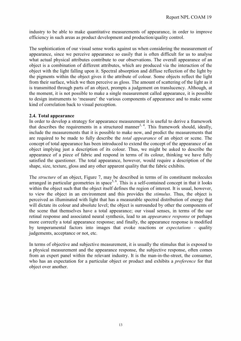
industry to be able to make quantitative measurements of appearance, in order to improve efficiency in such areas as product development and production/quality control. The sophistication of our visual sense works against us when considering the measurement of appearance, since we perceive appearance so easily that is often difficult for us to analyse what actual physical attributes contribute to our observations. The overall appearance of an object is a combination of different attributes, which are produced via the interaction of the object with the light falling upon it. Spectral absorption and diffuse reflection of the light by the pigments within the object gives it the attribute of colour. Some objects reflect the light from their surface, which we then perceive as gloss. The amount of scattering of the light as it is transmitted through parts of an object, prompts a judgement on translucency. Although, at the moment, it is not possible to make a single measurement called appearance, it is possible to design instruments to ‘measure’ the various components of appearance and to make some kind of correlation back to visual perception. 2.4. Total appearance In order to develop a strategy for appearance measurement it is useful to derive a framework that describes the requirements in a structured manner3, 4. This framework should, ideally, include the measurements that it is possible to make now, and predict the measurements that are required to be made to fully describe the total appearance of an object or scene. The concept of total appearance has been introduced to extend the concept of the appearance of an object implying just a description of its colour. Thus, we might be asked to describe the appearance of a piece of fabric and respond in terms of its colour, thinking we have fully satisfied the questioner. The total appearance, however, would require a description of the shape, size, texture, gloss and any other apparent quality that the fabric exhibits. The structure of an object, Figure 7, may be described in terms of its constituent molecules arranged in particular geometries in space5, 6. This is a self-contained concept in that it looks within the object such that the object itself defines the region of interest. It is usual, however, to view the object in an environment and this provides the stimulus. Thus, the object is perceived as illuminated with light that has a measurable spectral distribution of energy that will dictate its colour and absolute level; the object is surrounded by other the components of the scene that themselves have a total appearance; our visual senses, in terms of the our retinal response and associated neural synthesis, lead to an appearance response or perhaps more correctly a total appearance response; and finally, the appearance response is modified by temperamental factors into images that evoke reactions or expectations - quality judgements, acceptance or not, etc. In terms of objective and subjective measurement, it is usually the stimulus that is exposed to a physical measurement and the appearance response, the subjective response, often comes from an expert panel within the relevant industry. It is the man-in-the-street, the consumer, who has an expectation for a particular object or product and exhibits a preference for that object over another.

Report NPL COAM 19

14

Moleculesx

geometry

STRUCTUREx

environment

STIMULUSx

neural factors

APPEARANCEx

temperamentalfactors

STRUCTURE

STIMULUS

APPEARANCE

EXPECTATION

MEASUREMENT

EXPERT

CONSUMER

=

=

=

=

OBJECT

Physical effects

Psychophysicaleffects

Psychologicaleffects

Figure 7. A framework linking the neural and temperamental factors associated with appearance.

Another way of thinking of an object7 is to consider three aspects of appearance: physical, physiological and psychological, Figure 7. For instance, the gloss and colour of objects depend on the geometrical spatial distribution of light reflected by those objects (the physical aspect); this light distribution then stimulates the binocular human visual system, i.e. it provides a sensation (physiological aspects); and finally, thanks to long training, these sensations are interpreted by the cortex and recognised as objects (psychological aspects). Some synergy between these two ways of thinking is apparent in that the physical aspects are similar and measurable. The structure shown in Figure 7, however, ignores (or hides) the physiological aspects of appearance by assuming that their influence is on the appearance as interpreted by the visual response – the expert response. It is only after taking the

Report NPL COAM 19

15

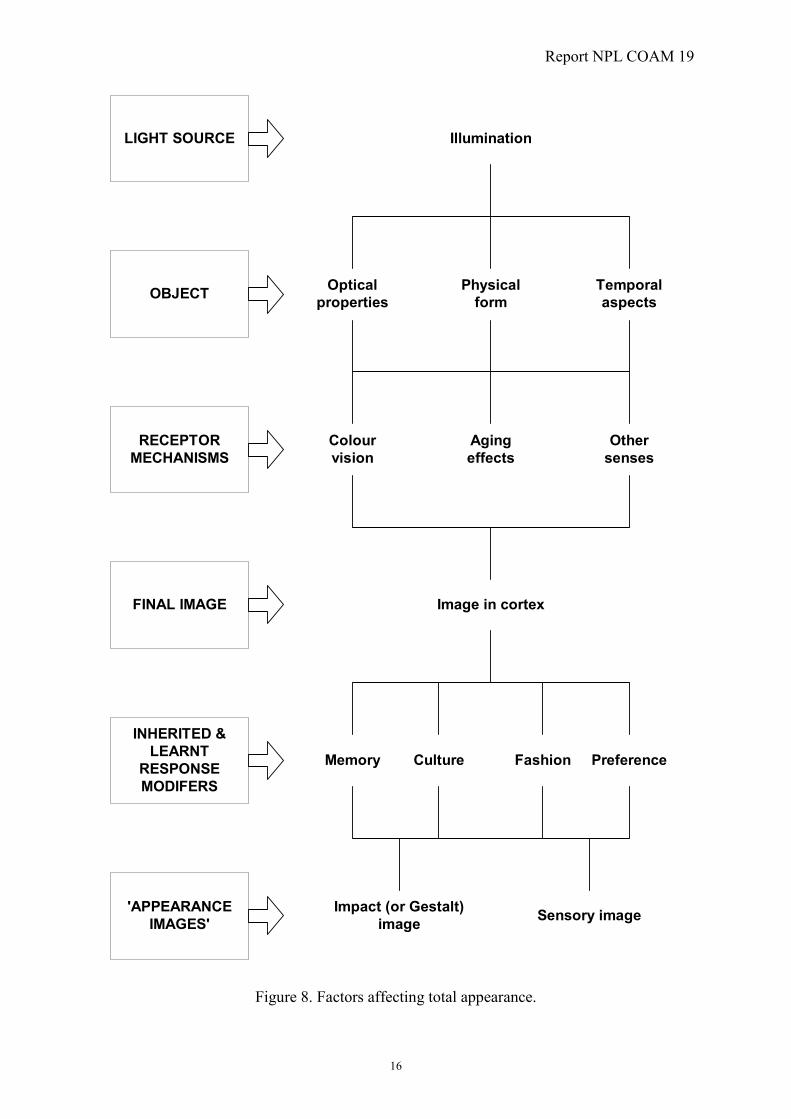
temperamental factors into consideration that this response is modified and the psychological response obtained. 2.5. Factors affecting total appearance At each of the lower three levels described in Figure 7, above, there are important factors that contribute to the response8. As already described, the light source that illuminates the scene has a spectral power distribution that defines the colour and absolute level of that illumination, Figure 8. The object itself has physical properties, optical properties, and temporal properties. The appearance response is influenced by the colour vision of the observer, ageing effects due specifically to the age of the observer, and the influence of responses from the other senses: hearing, smell, taste and touch. While these other responses are not considered as part of the framework for appearance measurement, their existence cannot be ignored because they influence any subjective data derived by observers. The final stage, that which defines the expectation of the observer, is influenced by many factors including the pre-conceptions of what the object should look like based on memory colour, cultural difference, what is in fashion, as well as our preference. The inference from the above is that ‘total appearance’ is a concept that is derived from a physical object or stimulus under the influence of the factors described by the various levels described by Figure 7 and Figure 8. In the real world, however, this is not the case because the appearance images come first – we see what we see – and base our responses and decisions on our interpretation of that image. Thus, Figure 8 could, with strong reason, be drawn the other way up!

Report NPL COAM 19

16

LIGHT SOURCE

OBJECT

RECEPTORMECHANISMS

INHERITED &LEARNT

RESPONSEMODIFERS

FINAL IMAGE

Illumination

Physicalform

Agingeffects

Othersenses

Colourvision

Opticalproperties

Temporalaspects

PreferenceFashionCultureMemory

Image in cortex

'APPEARANCEIMAGES'

Impact (or Gestalt)image Sensory image

Figure 8. Factors affecting total appearance.

Report NPL COAM 19

17

Hutchings9 suggests there are two classes of appearance images: the impact (or Gestalt) image, and the sensory image. The impact image is the initial recognition of the object or scene (the gestalt), plus an initial opinion or judgement. For the sensory appearance image, three hedonic descriptors are suggested for use, sensory, emotional and intellectual, that are used to prompt questions that should be asked of the image. For example, when eating a carrot, the sensory image contains an assessment of the visually perceived sensory properties – this jam will taste of strawberry. The emotional aspect might indicate that ‘we are eating this because we are celebrating my birthday’. The intellectual aspect might provoke the question ‘who cooked this cake?’ Thus, the concept of total appearance is indeed complicated, not least because of the multiple interactions between the various components of the process from object to expectation via visual response10. An example serves to illustrate this complexity. Tomatoes are perhaps initially perceived as being round red objects. Experience (memory – training) tells us that these are tomatoes, or at least they look like tomatoes (they might be real; they might be models). Depending on our expectation of the tomatoes, other responses are evoked. If we are in the supermarket and want to buy them then we might take particular notice of the colour and firmness as an indication of ripeness, the shine as an indication of freshness and the smell as an indication of sweetness. These responses are inter-related and their outcome leads to a decision based on the overall (perceived) quality; we either buy or not. Assuming a purchase is made then the decision is vindicated at home when the product is eaten because now the taste response, the flavour, the sweetness and the texture, all bear on our feeling of enjoyment (quality). As discussed above, it is unlikely that any physical scale called “appearance” will be possible and it is, therefore, necessary to look into the framework and find physical parameters that can be measured and the most obvious area for exploitation is that described in terms of the optical properties. 2.6 Discussion The above section attempts to provide a logical framework that describes the way in which the human observer responds to an external stimulus and, with the added benefits of both experience and memory, is able to make judgements about that stimulus in terms of its appearance. In order to ‘measure’ this concept called appearance, part of the framework includes the consideration of physical parameters that might correlate with the human response, Figure 7. The next section of this report will consider a further sub-division of the measurements into several different classes based on the optical properties of the object whose appearance in being assessed. In all of the discussion, several important considerations have been assumed. Most of these considerations might in themselves influence the final appearance of the object and so, in a complete assessment of appearance, need to be considered as variables in the system. It is reasonable for the sake of simplicity, however, and within the scope of this report, to consider these parameters as fixed, defined or constant. Our reaction to the appearance of an object is governed by the stimulus received by our senses and our response to that stimulus; the latter being the result of both physiological and psychological factors. It seems a reasonable assumption that physiological factors are

Report NPL COAM 19

18

common across racial, cultural and geographical boundaries, but the same can probably not be said for the psychological factors. The way a person responds to a stimulus is governed largely by his experience. It is highly likely that human experience does not have enough commonality to allow the development of universal measurement scales. Thus, each scale may relate only to a specific object as perceived by the members of a given society. In all situations requiring an assessment based on appearance it is a requirement that the object be lit, and the design of the lighting itself can either enhance or detract from the quality of the perceived object. A successful lighting design, whether it is daylighting or electric lighting or, as is more usual, a combination of the two, needs to satisfy a number of often conflicting requirements, one of which can be termed the visual function. This is a function of many parameters including:

�� the size of the light source, large and diffuse, or a point source, relative to the distance from the object – this will effect the highlights and shadows11,

�� the angular position of the light source, or sources, relative to the object and to the direction of view – this will effect the light modelling, as well as the highlights and shadows12,

�� the spectral distribution of the output of the source,

�� the level of illumination – as characterised by the brightness at the task area13,

�� the uniformity of that illumination over the task area,

�� the contrast between the task area and the surrounding area,

�� the amount of glare coming from extraneous light sources,

�� the colour performance of the light source14,

�� the presence of flicker from the light source15,

�� the reflectance of the object(s) to be lit16.

While for optimum appearance, each of these parameters needs to be optimised; there are other areas which must be considered in any good lighting design17. These include – in no particular order:

�� Energy efficiency

�� Installation maintenance

�� Capital and operational cost

�� Architectural integration

�� Visual amenity

Thus the lighting appearance of a scene, in which there is an area where a task has to be performed, can be an important additional consideration in any discussion of total appearance. Lighting can be regulated, but only to the extent that a number of Codes of Practice are available that provide recommendations for lighting specific scenes, both interior and exterior18. The concept of personal preference also plays an important part in many

Report NPL COAM 19

19

lighting installations especially for social use: for example, a low level of illumination may not be realistic for reading the menu in a restaurant, but it may be preferred from an aesthetic point-of-view! Preference is subjective and difficult to measure; suggestions have been made, however, for its definition when applied to practical applications19, 20. Another subject that has arguably been assumed in the above description is that of shape or form perception. This aspect of appearance also includes depth and motion perception. There are many different theories about how we recognise shapes21, 22, 23, 24:

�� Template theory – we have idealised templates stored in memory and we perform a match between these templates and the visual stimulus.

�� The Gestalt psychologist’s approach that emphasizes the whole context of an object and is not so interested in the individual elements of a scene but how they are all arranged together.

�� The information processing approach which focuses on a sequence of events and has the goal to try to understand each part of the sequence in terms of hierarchical organisation.

This latter theory attracts most support perhaps because it encompasses elements of the other two theories. Template theory requires only the knowledge of the shape of elemental parts of objects, the so-called primitive features. These can be both two-dimensional and three-dimensional, and it is assumed that the cortex ‘parses’ the image of the scene, a process known as perceptual parsing, and interprets its appearance in terms of the different primitives and their relationship one with another25. Gestalt theory has dominance over template theory because it requires not so much the recognition of templates but the understanding of the organisation of the whole scene: not the parts of the scene but the sum of those parts. Thus, the form or shape of an object is not perceived as a collection of its individual components but as a whole (Gestalt: a German word that means “entire figure”). As an example of a Gestalt interpretation, we recognise a television newsreader as a human being and assume that he/she has legs, even though they are not usually seen on the television screen. A mere analysis of the component parts of the image would not lead to this conclusion because the information perceived would be taken at face value. The size of an object, in its viewed environment, gives a clue as to the location of that object in a depth perspective and the temporal change of the object gives clues as to its movement (or not). Traditionally it has been assumed that depth perception is facilitated by the fact that the two two-dimensional images formed on the separate retinas of the two eyes are different and that the cortex uses the different information to construct the three-dimensional image of the scene. There are however, a number of monocular depth clues and an example is objects seen alongside receding railway lines. The parallel lines will converge in the distance, thus indicating where the distant point is and providing a suitable scaling point26.

Report NPL COAM 19

20

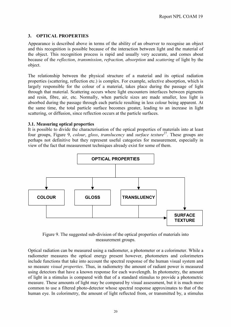
3. OPTICAL PROPERTIES Appearance is described above in terms of the ability of an observer to recognise an object and this recognition is possible because of the interaction between light and the material of the object. This recognition process is rapid and usually very accurate, and comes about because of the reflection, transmission, refraction, absorption and scattering of light by the object. The relationship between the physical structure of a material and its optical radiation properties (scattering, reflection etc.) is complex. For example, selective absorption, which is largely responsible for the colour of a material, takes place during the passage of light through that material. Scattering occurs where light encounters interfaces between pigments and resin, fibre, air, etc. Normally, when particle sizes are made smaller, less light is absorbed during the passage through each particle resulting in less colour being apparent. At the same time, the total particle surface becomes greater, leading to an increase in light scattering, or diffusion, since reflection occurs at the particle surfaces. 3.1. Measuring optical properties It is possible to divide the characterisation of the optical properties of materials into at least four groups, Figure 9, colour, gloss, translucency and surface texture27. These groups are perhaps not definitive but they represent useful categories for measurement, especially in view of the fact that measurement techniques already exist for some of them.

OPTICAL PROPERTIES

SURFACETEXTURE

TRANSLUENCYGLOSSCOLOUR

Figure 9. The suggested sub-division of the optical properties of materials into measurement groups.

Optical radiation can be measured using a radiometer, a photometer or a colorimeter. While a radiometer measures the optical energy present however, photometers and colorimeters include functions that take into account the spectral response of the human visual system and so measure visual properties. Thus, in radiometry the amount of radiant power is measured using detectors that have a known response for each wavelength. In photometry, the amount of light in a stimulus is compared with that of a standard stimulus to provide a photometric measure. These amounts of light may be compared by visual assessment, but it is much more common to use a filtered photo-detector whose spectral response approximates to that of the human eye. In colorimetry, the amount of light reflected from, or transmitted by, a stimulus

Report NPL COAM 19

21

can be detected using three photo-detectors whose individual spectral response approximates to the colour responses of the human eye28. These measurements can also be made spectrally by measuring the amounts of radiation using narrow bands of wavelengths situated at regular intervals throughout the spectrum. The photometric and colorimetric parameters are then calculated using tables of data corresponding to the appropriate spectral responses. Thus, the human perceptual attribute, the ‘colour’, of a sample can be ‘measured’ and its position relative to any other colour located on a colour map. This type of measurement is of importance, for example, in assessing whether the colour of a signal light is appropriate. To be correct, the measured colour must fall within a defined area on the colour map and this area is usually specified by an appropriate standard. There should be no overlap between the areas designated for different coloured signals to avoid confusion to the observer. An obvious application is in railway signalling where red signals from different manufacturers may appear to have a slightly different colour but their measured colours must all fall within the designated area of the colour map. Thus, to the train driver they should all appear ‘red’. What is often of more interest to industry is not the absolute colour of a sample but the relative ‘colour-difference’ between a reference sample and a test sample. In the clothing industry, for example, a cloth sample swatch might be provided and a dye-house required to dye fabric to match. While an instrument can measure the colour of both pieces of fabric in an absolute sense, it can also calculate the colour-difference between them, on a scale that correlates with the colour difference perceived by a human observer.

Report NPL COAM 19

22

4. MEASURING COLOUR There are three ways of measuring colour. The first is by using the human eye and an example of a visual colorimeter is the Lovibond Tintometer designed to optimise the use of Lovibond glass filters29. Originally constructed to measure the colour of beer, it relies on three sets of glasses that are uniformly graded to provide a continuous scale in red, yellow and blue. The observer makes a match between combinations of these glasses and the object whose colour is being monitored. The result is then expressed in terms of the amounts of the three glasses. As such, this can be considered to be a measurement of the appearance of the object, for example a particular sample may be matched as 25 Yellow 10 Red. While this instrument has found wide acceptance in the brewing, edible oil, petroleum spirit, honey, tallow and fats, rosins and resins industries, it relies on the individual observer to make the match and thus represents a simple and, at present, non-traceable means of measuring colour. An interesting extension of this visual colorimeter is the establishment of a large number of one-dimensional scales for specific products. Examples are the European Pharmacopoeia scales30, 31 for the pharmaceutical industry, Figure 10, the Gardner scale for resins32, the ASTM D1500 scale for petroleum oils33, the ICUMSA scale for sugars34, the EBC Scale for beer35, the Platinum-Cobalt/Hazen/APHA Colour Scale for water36, and the US Navel Stores Scale for rosins37. These scales are truly appearance scales in that a series of glasses are designed to visually match the range of a specific product.

0.30

0.35

0.40

0.45

0.30 0.35 0.40 0.45 0.50

x

y

Red Yellow Brow n

Brow nish-Yellow Greenish-Yellow

(a)

Report NPL COAM 19

23

0

10

20

30

40

50

60

-20 -10 0 10 20 30 40

CIELAB a*

CIE

LAB

b*

Red Yellow BrownBrownish-Yellow Greenish-Yellow

Figure 10. The 5 colour scales of the European Pharmacopoeia standards plotted in (a) the x, y chromaticity diagram and (b), the a*, b* diagram.

Figure 11. The fundamental components that enable colour perception.

(b)

Report NPL COAM 19

24

4.1 CIE colorimetry In order to measure the colour of an object more rigorously, three things must be characterised: the light source used to illuminate the object, the spectral absorption properties of the object and the spectral response of the human eye, Figure 11. The CIE (Commission Internationale de L’Eclairage) has specified a helpful measure of the light source and the observer, and the measurement of the spectral reflectance (or transmittance) can be made using a suitable spectrophotometer38.

0

50

100

150

200

250

350 400 450 500 550 600 650 700 750 800

Wavelength nm

Rel

ativ

e sp

ectr

al p

ower

SAD65

Figure 12. Relative spectral power distributions of CIE standard illuminants D65 and SA.

0.0

0.2

0.4

0.6

0.8

1.0

1.2

1.4

1.6

1.8

2.0

350 400 450 500 550 600 650 700 750 800

Wavelength nm

Rel

ativ

e re

spon

se

x bar

y bar

z bar

Figure 13. The CIE colour-matching functions for the 1931 Standard Colorimetric Observer.

Report NPL COAM 19

25

The CIE recommends the use of two standard illuminants: one representing a phase of daylight with a correlated colour temperature of 6500K (D65) and a second representing incandescent illumination (SA), Figure 12. While these might not be real sources of illumination – they are presented as tables of data – their use implies consistency wherever in the world the measurements are made. Similarly, the CIE has been able to specify the response characteristics of a ‘standard observer’, based on early experimental work involving 20 observers at Imperial College and at NPL, Figure 13. By integrating the spectral reflectance data, R(�), with that of the illuminant, S(�), and the observer, )(z),(y),(x ��� , three numbers, the tristimulus values, X, Y, Z, are obtained that uniquely define a colour as viewed in the given environment:

���

�����

�����

�����

d)(z)(S)(RkZ

d)(y)(S)(RkY

d)(x)(S)(RkX

� ���� d)(y)(S/kwhere 100 The CIE system is configured such that the Y tristimulus value correlates approximately with brightness or, more usually with lightness (relative brightness). The X and Z tristimulus values, however, have no perceptual correlates. Important colour, or chromaticity attributes can however, be related to the relative magnitudes of the tristimulus values and it is therefore helpful to calculate the chromaticity coordinates:

)ZYX/(Yy)ZYX/(Xx

���

���

The original CIE 1931 x, y chromaticity diagram provides a convenient way of mapping the positions of coloured samples relative to the position of the ‘white’ light that is used to illuminate them, Figure 14. The boundary of this diagram, the spectrum locus, is the locus of points that represent monochromatic stimuli throughout the spectrum. It has been found, however, that the sensitivity of the eye to colour differences varies in different parts of the chromaticity diagram, and in particular, in the green region quite large changes in position are not very obvious visually. To correct this, the diagram can be altered in shape so that equal distances more nearly represent equal perceptual steps. This led to the CIE 1976 u’, v’ chromaticity diagram.

Report NPL COAM 19

26

0.0

0.1

0.2

0.3

0.4

0.5

0.6

0.7

0.8

0.9

0.0 0.1 0.2 0.3 0.4 0.5 0.6 0.7 0.8

CIE chromaticity x

CIE

chr

omat

icity

y

SL

D65

SA

Figure 14. The CIE x, y chromaticity diagram.

Chromaticity diagrams have many uses, but, as they show only proportions of tristimulus values, and not their actual magnitudes, they are only strictly applicable to colours having the same luminance. In general, colours vary in both chromaticity and luminance, and some method of combining these variables is therefore required. To meet this need, the CIE has recommended the use of one of two alternative colour spaces, designated CIELAB colour space and CIELUV colour space, and it is the former that has found favour in the world of surface colours. The coordinates of CIELAB colour space are L*, a*, and b*, and these are, or can be combined to be, correlates of the perceptual quantities, lightness, chroma and hue. There is also a colour-difference formula associated with both spaces39, 40. L* = 116 (Y/Yn)1/3 – 16 Y/Yn > 0.008856

L* = 903.3 (Y/Yn) Y/Yn <= 0.008856

a* = 500 [f(X/Xn) - f(Y/Yn)]

b* = 200 [f(Y/Yn) - f(Z/Zn)]

where f(X/Xn) = (X/Xn)1/3 X/Xn > 0.008856

f(X/Xn) = 7.787(X/Xn) + 16/116 X/Xn <= 0.008856

f(Y/Yn) = (Y/Yn)1/3 Y/Yn > 0.008856

f(Y/Yn) = 7.787(Y/Yn) + 16/116 Y/Yn <= 0.008856

f(Z/Zn) = (Z/Zn)1/3 Z/Zn > 0.008856

f(Z/Zn) = 7.787(Z/Zn) + 16/116 Z/Zn <= 0.008856

C*ab = (a*2 + b*2)1/2

hab = arctan (b*/a*)

Report NPL COAM 19

27

+ a*

- a*

+ b*

- b*

C*ab constant hab constant

L*

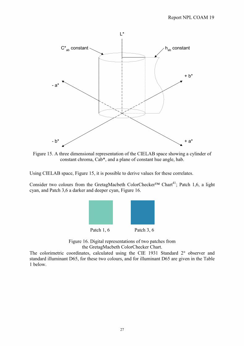
Figure 15. A three dimensional representation of the CIELAB space showing a cylinder of

constant chroma, Cab*, and a plane of constant hue angle, hab.

Using CIELAB space, Figure 15, it is possible to derive values for these correlates. Consider two colours from the GretagMacbeth ColorChecker™ Chart41; Patch 1,6, a light cyan, and Patch 3,6 a darker and deeper cyan, Figure 16.

Patch 1, 6 Patch 3, 6

Figure 16. Digital representations of two patches from the GretagMacbeth ColorChecker Chart.

The colorimetric coordinates, calculated using the CIE 1931 Standard 2� observer and standard illuminant D65, for these two colours, and for illuminant D65 are given in the Table 1 below.

Report NPL COAM 19

28

Table 1. Colorimetric coordinates for patches (1, 3), (3, 6) and illuminant D65. (1, 6) (3, 6) D65 Tristimulus values X 31.5 15.0 95.6 Y 43.1 20.3 100.0 Z 45.3 41.0 109.7 1931Chromaticity coordinates x 0.2629 0.1963 0.3131 y 0.3593 0.2662 0.3276 1976 Chromaticity coordinates u’ 0.1550 0.1353 0.1986 v’ 0.4766 0.4129 0.4676 1976 Uniform colour scale L* 71.63 52.16 100.0 coordinates (CIELAB) a* -32.18 -24.31 0.0 b* 2.11 -26.53 0.0 C* 32.24 35.98 0.0 h 227� 176� 0.0

The chromaticity coordinates can be interpreted by plotting on a chromaticity diagram but the easiest way to interpret the data, and the appearance of the colours, is to consider the CIELAB coordinates. The following can be deduced: �� Patch (1, 6) is lighter than Patch (3, 6) – L* = 71.63 is greater than L* = 52.16 �� Patch (1, 6) is slightly lower in chroma than Patch (3, 6) – C* = 32.24 is less than C* =

35.98 �� Patch (1, 6) is bluer than Patch (3, 6) – 227� is closer to 300�, the approximate position

of unique blue. �� Conversely, Patch (3, 6) is greener than Patch (1, 6) – 176� is on the green side of 227�. Notice that these deductions are relative: it is not possible, using CIE colorimetry, to deduce anything about the absolute appearance of the coloured patches. 4.1. Colour appearance Traditional CIE colorimetry has been with us for a long time – the CIE 1931 Standard Colorimetric Observer celebrated its 70th birthday in 2001! The CIE system of colour measurement, based as it is on the colour matching functions that represent the standard observer, has stood the test of time and proved to be of immense value in helping to solve many measurement problems. As one of the ‘fathers’ of the Standard Observer, David Wright, has so aptly pointed out, however: “The definition of a colour by its X, Y, Z tristimulus values, although it involves an observer and is therefore based on subjective observation does not in itself define the appearance of the colour.42” 4.2. Colour appearance models The situation can be imagined where there are two colours, both specified in terms of their tristimulus values, and it is required to know their difference in appearance when viewed

Report NPL COAM 19

29

under the same specified viewing conditions. Some approximate estimates can be obtained by transforming the tristimulus values to chromaticity coordinates and plotting these values on a chromaticity diagram together with the position of the appropriate white point. In this way a relative idea can be obtained as to whether one sample is, for example, redder than another, and which sample has the higher purity. No information is available, however, as to their absolute colour appearances. Within the last 20 years much progress has been made to derive models of colour appearance that provide both absolute and relative correlates that relate to the appearance of objects. A colour appearance model should comprise at least three stages, Figure 17: a chromatic adaptation transform, a dynamic response model and a colour space for representing the correlates of the percepts43. The purpose of the chromatic adaptation transform is to allow tristimulus input data for any illuminant. A transformation is then made to give the equivalent tristimulus values for the illuminant used by the model, usually Illuminant D65 or Illuminant SE. This might carry out a normalisation in cone response space and currently there is no recommended method for making this step. There are several chromatic adaptation transforms that seem to work moderately well and none can be clearly defined as the best, based on available data for evaluation. Thus, there is no CIE recommended transform. CIE have however, produced a report that discusses the situation and presents the most efficient transforms44.

Report NPL COAM 19

30

The COLOUR element

The SURROUND field

The BACKGROUND

Effect of CHROMATICADAPTATION

CONE RESPONSEFUNCTIONS

PERCEPTUALCORRELATES

Redness-greennessYellowness-blueness

HueBrightness

Colourfulness

HueLightness

Croma

Saturation

The level ofILLUMINATION

Figure 17. Block diagram showing the building blocks of a colour appearance model.

Under a given set of viewing conditions, there will be a predictable relationship between the responses of the cones in the human retina and the intensity (magnitude) of the stimulus and there is much evidence to suggest that this relationship is non-linear. If the cone responses are taken to be related to the stimulus intensity by a power function then the observed reduction in dynamic range is adequately predicted. When the intensity of the stimulus is very low, noise in the system must prevent extremely small cone responses from being significant; and,

Report NPL COAM 19

31

when the intensity of the stimulus is very intense, the response must eventually reach a maximum and the power function cannot predict this. For this reason a hyperbolic function is often chosen as the dynamic response function: there is some physiological evidence for the existence of such a function in the retina45, Figure 18.

-1.0

-0.5

0.0

0.5

1.0

1.5

2.0

2.5

3.0

-4.0 -3.0 -2.0 -1.0 0.0 1.0 2.0 3.0

Log (Input radiation)

Log

(Con

e re

spon

se)

Square root

Hyperbolic

Figure 18. Cone response function. The log of the function is plotted against the log of the

input radiation.

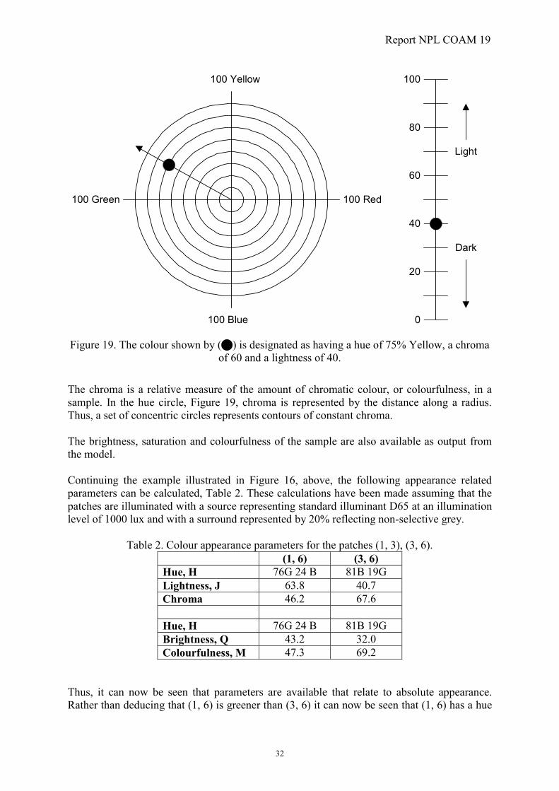
A model of colour vision, first proposed by Hunt in 198246, has provided a basis for predicting colour appearance that is in good agreement with available data including established colour order systems (for example, the Swedish Natural Color System47). The basic model provides predictions of colour appearance using illuminants other than daylight and the input data includes the colour and absolute level of the illumination and the colour of the surround to the sample of interest. The output of the model includes the hue, the lightness and the chroma of the measured sample. The hue of a coloured sample can be expressed in terms of the psychological primaries: red, yellow, green and blue. These four unique hues can be represented as the points on a hue circle, Figure 19. The hue of a coloured sample can then be expressed as a unique hue, e.g. 100% red, or as a mixture of two adjacent unique hues, e.g. a turquoise colour may be 60% blue and 40% green. The hue can also be represented as a continuous scale of 0 to 400 where 0 represents unique red, 100 unique yellow, 200 unique green and 300 unique blue. On this scale the hue of the turquoise sample would be 260. The lightness may be thought of as a measure of relative brightness, i.e. the brightness of a colour relative to the brightness of a similarly illuminated white in the same scene. If the latter is scaled as 100, all other colours can be attributed numbers between zero (black) and 100, Figure 19.

Report NPL COAM 19

32

100 Red100 Green

100 Yellow

100 Blue

Light

Dark

100

80

60

40

20

0

Figure 19. The colour shown by (�) is designated as having a hue of 75% Yellow, a chroma of 60 and a lightness of 40.

The chroma is a relative measure of the amount of chromatic colour, or colourfulness, in a sample. In the hue circle, Figure 19, chroma is represented by the distance along a radius. Thus, a set of concentric circles represents contours of constant chroma. The brightness, saturation and colourfulness of the sample are also available as output from the model. Continuing the example illustrated in Figure 16, above, the following appearance related parameters can be calculated, Table 2. These calculations have been made assuming that the patches are illuminated with a source representing standard illuminant D65 at an illumination level of 1000 lux and with a surround represented by 20% reflecting non-selective grey.

Table 2. Colour appearance parameters for the patches (1, 3), (3, 6). (1, 6) (3, 6) Hue, H 76G 24 B 81B 19G Lightness, J 63.8 40.7 Chroma 46.2 67.6 Hue, H 76G 24 B 81B 19G Brightness, Q 43.2 32.0 Colourfulness, M 47.3 69.2

Thus, it can now be seen that parameters are available that relate to absolute appearance. Rather than deducing that (1, 6) is greener than (3, 6) it can now be seen that (1, 6) has a hue

Report NPL COAM 19

33

of 76% green and 24% blue, whereas (3, 6) has a hue of 81% blue and 19% green – a difference of 57 hue units. Note that the use of hue, brightness and colourfulness is useful when comparing the appearance of the same colour under different levels of illumination. The values of these parameters will increase with increasing level whereas those for the relative parameters, hue, lightness and chroma will stay approximately constant. At a CIE meeting, held in Kyoto, Japan, in 1997, CIE agreed to recommend the CIECAM97s colour appearance model for further evaluation48. This model depends on the work of many different investigators, including Nayatani and his co-workers from Japan, Berns and Fairchild from the USA, and Hunt and Luo and their co-workers from the UK. The main strengths of the model are as follows49: �� It relies on much physiological data and hence includes the minimum of empiricism.

�� While not perhaps definitive, it represents the best available model.

�� It has international acceptance.

�� Its application in colour management systems in the colour reproduction industry has been successful.

The main negative response to the model concerns its complexity. That this is so was almost inevitable because the human visual system, which the model attempts to imitate, is known to be very complex; so complex that it is not yet fully understood from a physiological point-of-view. There are parts of the model that now require change to improve the prediction to experimental data; indeed, there are many new sets of experimental data. It is thus likely that there will be a new version of the model, recommended by CIE, in the near future50, 51, 52. In addition, there are now moves to progress from colour appearance models to image appearance models. The objective in formulating such a model is to simultaneously provide traditional colour appearance capabilities, spatial vision attributes and colour difference metrics, in a model simple enough for practical applications53. Another short-coming of the recommended colour appearance model is that it defines a white point to which it is assumed the eye is totally adapted. There are, however, some real situations where the eye is viewing two scenes, perhaps by moving the field-of-view from one to the other. If these two scenes have different white points then the eye has to adapt to an intermediate point and will not be totally adapted to either. An example of such a scene is to be found in the world of colour printing, graphic arts, where a soft copy proof may be viewed on a computer monitor with a white point defined as having a correlated colour temperature of 9300 K. A hard copy reproduction is typically viewed in a booth having a correlated colour temperature equivalent to CIE illuminant D50. It has been shown that the eye adapts approximately 40% to the monitor and 60% to the viewing booth54, 55, 56, 57. This represents a mixed-adaptation situation and needs to be included in a future colour appearance model if it is to be successfully applied to the colour image reproduction chain. 4.3. Discussion – colour Thus, the ‘appearance’ of a coloured sample can be well described, at least within the confine of the latest colour appearance model. Traditional colour measuring instruments, usually

Report NPL COAM 19

34

measuring spectral data and based on diffraction grating monochromators with photo-diode array detectors, provide an adequate means of measuring CIE tristimulus values. The conversion to colour appearance parameters is dependent on the environment in which the coloured sample is viewed, the viewing conditions, and to calculate these numbers additional data are needed, including the absolute level of the illumination and the colour of the surround to the sample. A colour measurement system based on digital imaging could provide these data leading to output in terms of colour appearance variables after suitable calculation. There are at least two other variables that influence the appearance of a coloured sample and that are not implicitly considered in the above description. These are the effect of variation in angles of illumination and detection of the light incident onto, and reflected from, the sample respectively, and the effect of local variation, or non-uniformity of the physical surface that is being measured. 4.3.1. Geometry It is common experience that the appearance of coloured samples varies with the direction of the illumination and viewing. If surfaces were perfectly diffuse and uniform, this would not happen. But most surfaces have some gloss or sheen (to be discussed explicitly later in this report). The gloss results in some of the incident light being reflected without passing through the colorant and it therefore desaturates the colour, the amount of desaturation being dependent on the angles of illumination and viewing. To expedite a measurement process, the CIE has recommended two basic systems of geometry that are usually implemented in measuring instruments58. The first requires the specimen to be illuminated at an angle of 45� � 5� from the normal to that surface and viewed in the direction normal to the surface, Figure 20. This is known as 45/0 geometry and the converse 0/45 geometry is also permitted. In the second configuration the sample is illuminated diffusely by an integrating sphere and then viewed along a line at approximately 8� to the normal to the surface; a configuration known as d/8 geometry. Again the converse geometry, 0/d is permitted.

Report NPL COAM 19

35

45/0 0/45

0/dd/8

IlluminationIllumination

Illumination

Illumination

ViewingViewing

Viewing

Viewing

Figure 20. The configuration of d/8, 0/d, 45/0 and 0/45 illuminating/viewing geometries as

recommended by the CIE.

It is seen in the above discussion that the geometries of both illumination and collection of the light are considered together. There are, however, many surfaces that cannot be adequately measured using such limited conditions – the so-called gonio-apparent or special- effect colours59, 60. A popular example is the often coloured, metallic finish applied to many automobiles61, 62. This changes its appearance according to the angle of illumination and viewing and, for complete characterisation, should have the colour measured at more than one illumination/viewing angle combination63, 64. To use an integrating sphere is a compromise in that it might capture the average colorimetry of the sample but not the detailed variation of the colour with angle. This limitation has been partly overcome by the introduction of so called multi-angle spectrophotometers, which measure at more than one, and typically four or five angles, Figure 2165.

Report NPL COAM 19

36

110degrees

75degrees

25degrees

Illumination Specular angle

15degrees

45degrees

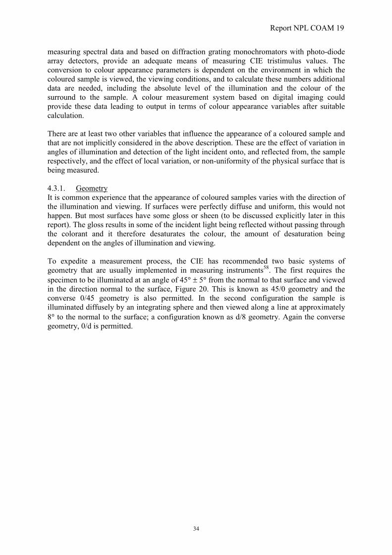
Figure 21. Multi-angle spectrophotometry – viewing angles are measured with respect to the aspecular angle.

Note that these instruments use the concept of aspecular angle and rather than designating the angles from the normal to the sample surface, designate them with respect to the specular angle66, Table 3.

Table 3. The designation of incident and viewing angles for multi-angle spectral measurements.

Angle designated with respect to the aspecular

angle

Angle designated with respect to the normal the surface to be measured

Angle designated with respect to the surface to

be measured Incident - illumination Incident – illumination Incident – illumination

90� 45� 45�

Viewing - detection Viewing – detection Viewing - detection 15� -30� 120� 25� -20� 110� 45� 0� 90� 75� 30� 60� 110� 65� 25�

The figures shown in bold in Table 3 are the angles used to describe the measurements made using commercially available multi-angle spectrophotometers: it is seen that they are a mixture in that the viewing angle is designated with respect to the normal to the surface and the viewing angles with respect to the aspecular angle. The left-hand column of the table shows the values of the angles designated with respect to the normal to the surface to be measured. A more convenient system may be as shown in the right-hand column where the angles are designated with respect the surface to be measured – this system negates the use of negative numbers and is likely to be more convenient when it becomes necessary to measure at more than 5 angles – see below.

Report NPL COAM 19

37

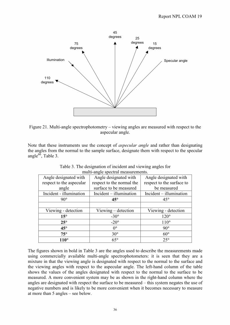
For many surfaces, notably some of the pearlescent67, 68 and interference69, 70, 71, 72, 73, 74, 75, 76, 77 pigments that are now being used for product finishes, the limitation to four angles78 is probably insufficient and the use of a goniospectrophotometer becomes necessary79, 80. This instrument, which can be considered as an extended goniophotometer as used in the measurement of the light distribution from, for example, a luminaire, enables the sample to be illuminated from any angle and viewed over a wide range of angles, often by scanning a range from � 85� to the normal to the surface. While such instruments are commercially available, their use is not widespread partly perhaps due to their relatively high cost, and the lack of a standard procedure for making multi-angle measurements81, 82. In order to differentiate between current multi-angle instruments, which measure at four or five angles, and goniospectrophotometers, it might be useful to classify the former ‘four (or five)-angle spectrophotometers’ and keep the designation ‘multi-angle’ for the true gonio instruments. New methods are going to be needed to represent the large amount of data that can be generated from a goniospectrophotometric instrument. Obviously, plots of the spectral data will be of use, but the colorimetry, and colour appearance parameters, derived from those spectral data are of greater value.

0

100

200

300

400

500

600

-45 -30 -15 0 15 30 45 60 75 90 105 120 135

Viewing (aspecular) angle

CIE

LAB

ligh

tnes

s L*

SolidPearlMetal

Figure 22. CIELAB lightness, L*, plotted as a function of the aspecular angle at which the

spectral measurement was made: illumination at 45� to the normal to the surface – equivalent to 90� aspecular angle. Data are shown for a solid colour, a metallic pigment

and a pearlescent pigment.

Report NPL COAM 19

38

Figure 22 shows a series of measurements made using a goniospectrophotometer of a number of samples made using different pigments: CIELAB lightness, L*, is plotted as a function of the viewing (aspecular) angle. The gap in the data from 65� to 105� represents the position of the illuminating beam of light. It is seen that the lightness of the solid colour does not significantly change with viewing angle. The lightness of the metallic pigment changes from approximately 12 near to the illuminating beam to over 100 close to the specular beam and over 500 at the specular position. A similar trend is exhibited by the pearlescent pigment although the lightness close to the illumination beam is higher, at approximately 75, than that of the metallic pigment at the same angle. It should be noted that both the metallic and pearlescent pigments are over-coated with an acrylic lacquer to give a high gloss finish.

0

50

100

150

200

250

300

-45 -30 -15 0 15 30 45 60 75 90 105 120 135

Viewing (aspecular) angle

CIE

LAB

hue

ang

le h

Solid

Pearl

Metal

Figure 23. CIELAB hue angle, h, plotted as a function of the aspecular angle at which the

spectral measurement was made: illumination at 45� to the normal to the surface – equivalent to 90� aspecular angle. Data are shown for a solid colour, a metallic pigment

and a pearlescent pigment. Figure 23 shows the same series of measurements as shown in Figure 22 but with CIELAB hue angle, h, plotted as a function of the viewing (aspecular) angle. It is seen that the hue of the solid colour does not significantly change with viewing angle. The hue of the metallic pigment changes from approximately 270� near to the illuminating beam to 230� close to the specular beam: this change indicates the appearance of the material taking on the colour of the illuminant as the viewing angle approaches the specular position. The hue of the pearlescent pigment, however, changes from 100� close to the illuminating position, to 220� close to the specular position indicating a change in hue from yellowish-green to bluish-green83.

Report NPL COAM 19

39

One measure that has been suggested is the Flop Index developed by Alman84 who had observers rate the perceived flop of several metallic car panels as the sample was rotated through the entire range of viewing angles. A solid colour has a value of zero and the very high flop of a metallic coating has a value in the range 15 to 17. An equation for the Flop Index was derived based on the measurement angles recommended by DuPont and constructed in terms of the CIE Lightness, L15*, L45* and L110*, calculated from the reflectance measurements at the three angles 15�, 45� and 110�, respectively85:

Flop IndexL LL

�

�2 69 15 1101 11

450 86

. ( )( )

* * .

* .

Figure 24 shows a typical plot of CIELAB Lightness, L*, as a function of measurement angle for a metallic paint sample2; the associated value of Flop Index is approximately 14.

0

20

40

60

80

100

120

140

0 20 40 60 80 100 120Measurement Angle

CIE

Met

ric L

ight

ness

, L*

Figure 24. CIELAB Lightness, L*, as a function of measurement angle for a metallic sample.

A second measure, based on goniospectrophotometric measurements, has been presented by the makers of the ChromaFlair� pigments as a method of describing the high colour gamut associated with these products86. A series of readings of CIELAB a* and b* values is obtained as a function of measurement angle, typically from 10 to 60 degrees in steps of 5 degrees. Lines are drawn connecting the respective a*, b* values, Figure 25, and the end points are connected to the achromatic point given by a*, b* = 0, 0. The Dynamic Colour Area, DCA�, metric is then given by the area of the shape so defined. It should be noted that the outer boundary of this shape, as defined by the values of a*, b*, defines the change in perceived colour with change in angle. Thus, the pigment represented in Figure 25 is a cyan/purple/red pigment.

Report NPL COAM 19

40

-80

-60

-40

-20

0

20

40

60

-40 -20 0 20 40 60 80 100

CIELAB a*

CIE

LAB

b*

Figure 25. ChromaFlair� dynamic colour area defined in CIE a*, b* uniform colour space.

These new parameters are useful in that they both attempt to correlate with visual percepts, the flop index to the lightness and the dynamic colour area to the angular change in hue/chroma. They do not capture, however, all of the variation that can be defined from gonio measurements. To do this, it might be necessary to selectively plot the data to enable the rate of change of the separate parameters to be observed; it might be necessary to define new parameters. It is also necessary to consider the colour difference between gonio-apparent samples and it is unlikely that the usual colour-difference equations can be applied. Nicholls87 has suggested an equation based on measurements at three angles together with a measurement based on specular included (diffuse) geometry. DIN has recently published a standard defining methods for colour measurement using four specular angles: 25�, 45�, 75� and 110�. An associated colour-difference formula uses different scaling factors to separately weight the contributions of the lightness, chroma and hue differences to the overall colour difference at each angle88. 4.3.2. Non-uniformity and surface texture The presence of non-uniformity and surface texture can make the colour of the sample vary as it is rotated or translated in its own plane and this will occur with any interlaced material such as textiles, and with tufted materials such as carpet. In addition, there are products such as aluminium (as used for drinks cans), knitted fabrics, metallic car finishes, and many decorative and natural surface finishes that are textured. It should be noted that two types of surface texture can be identified. Car finishes use a pigment layer that is itself textured but is protected by an overcoat of acrylic varnish. Thus, the physical surface is smooth while the visual appearance is of texture: this can be referred to as optical texture. The drinks can, however, has a physical topology that is not smooth and this effect is referred to as physical texture89. It should be further noted that both of these definitions of surface texture require there to be visible mechanical structure to the surface. Any purely colour non-uniformity is referred to as colour uniformity or colour patterning. Thus, although the same mathematical analysis methods might be used for both aspects of non-uniformity, it is clearly recognised

Report NPL COAM 19

41

that there is a difference between colour patterning due only to colour, and colour patterning due to surface texture. The percept of surface texture will be discussed in a later section of this report where it will be noted that an electronic image-capturing device, for example a digital camera, can be used to aid the ‘measurement’ of texture. This is possible because the device has the ability to capture a large amount of data in a spatial sense. It should also be possible to use a digital camera to ‘measure’ the colour appearance parameters, described above. Because the camera is a spatial recording device, it can capture an image that includes not only the coloured object whose appearance requires measurement, but also information about the colour of the surround to the object and, if a suitable white reference object is placed in the field-of-view, information about the colour of the illuminant. If a suitable calibration is available then the absolute level of this illumination can be recorded giving all of the information that is required to compute the appearance parameters. Digital cameras record information using device dependent R, G, B values that can be considered analogous to X, Y, Z tristimulus values. R, G, B values are device dependent because different manufacturers’ cameras have different values of spectral response; X, Y, Z tristimulus values however, are independent of the device because they rely on only the spectral response of one of the CIE standard colorimetric observers for calculation90. Procedures are available for characterising digital cameras to derive a matrix that will convert the device R, G, B values to approximate CIE X, Y, Z tristimulus values91, 92, 93. Note that, in the world of food processing, the term texture has a different meaning94. Here, texture is concerned with the feel of food in the mouth and is an important parameter in the assessment of different food products by the perception of the structural properties. Thus, the perception of moisture, size, shape and roughness of food particles are important factors influencing texture sensations95, 96. It is mainly for this reason that the percept of texture is termed surface texture in the above discussion concerned with total appearance.

Report NPL COAM 19

42

5. GLOSS APPEARANCE Gloss perception is associated with the way that an object reflects light, particularly depending on the way that light is reflected from the surface of the object at and near the specular direction. Gloss is normally perceived independent of colour; it may, however, be affected by the underlying colour of the object or itself affect the perceived colour of the object. It is usual, however, for the perception of gloss to be abstracted from the total visual experience as separate from colour. Hunter97 first defined specular gloss as the ratio of the light reflected from a surface at a specified angle to that incident on the surface at the same angle on the other side of the surface normal, Figure 26. Hunter recognised, however, that the perception of gloss requires more than just consideration of the specular reflection.

S

I

I

I S

I

I

Sh

S

S

D

D B

Specular gloss

Sheen

Contrast gloss or lustre

Distinctness-of-image gloss

Absence-of-bloom gloss

G � S/I

G � �S/I

G � D/S

G � (B-D)/I

G � dR/d�

Figure 26. Hunter’s five types of gloss.

Report NPL COAM 19

43

Sheen was defined as gloss at grazing angles of incidence and viewing; contrast gloss or lustre as the ratio of the specularly reflected light and that diffusely reflected normal to the surface, absence-of-bloom as a measure of the absence of haze or a milky appearance adjacent to the specularly reflected light; and distinctness-of-image as the sharpness of the specularly reflected light. Thus, a surface can appear very shiny if it has a well-defined specular reflectance at the specular angle. The perception of an image reflected in the surface can be degraded by appearing unsharp, or by appearing to be of low contrast, Figure 27. The former is characterised by the distinctness-of-image and the latter by the haze or contrast gloss (haze is the inverse of absence-of-bloom)98. An added complexity is due to surface non-uniformity leading to an effect known as orange peel. This effect can be caused, for example, by uneven coating of the acrylic overcoat on an automobile finish leading to a relatively low frequency ‘ripple’. It should be noted that it is not always the ‘top’ surface of a material that contributes to the gloss. The quality of the colour image produced by inkjet printing technology, for example, varies depending on the type and quality of the substrate, the raw stock paper99. To get a high laydown of ink requires a relatively rough surface to give a high surface area on which to print; this, however, tends to be a relatively low gloss surface and so the print will not look ‘photographic’ or have a high gloss.

0.0

0.2

0.4

0.6

0.8

1.0

-2.0 -1.0 0.0 1.0 2.0

Offset angle from specular

Ref

lect

ed in

tens

ity

Figure 27. Examples of distinctness-of-image measurements at three levels of gloss.

Harrison100, after extensive studies in which the ability of individual observers to rank a range of surfaces according to their gloss was compared with instrumental measurements, has concluded that the gloss of surfaces is not a simple physical property but a psychological Gestalt, that is an appraisal of the physical situation taken as a whole. It was found that observers tend to fall in to one of two categories. In the first, observers judge gloss with reference to the total amount of light reflected from a surface, whilst the others judge gloss according to the sharpness of images seen via the reflecting surface. The only other ‘historic’ comprehensive study of visual gloss scaling is that made by O’Donnell and Billmeyer101. Painted panels were prepared with a wide range of gloss and three achromatic colours (white, grey and black) by varying the composition and heat

Report NPL COAM 19

44

treatment of an automobile acrylic lacquer system. Magnitude scaling was used to estimate the visual dissimilarities between members of all possible pairs of specimens in series of 15-20 samples. The data were analysed using multidimensional scaling techniques. Measurements were also made using a conventional three-angle gloss meter (described below). It was considered conceivable that observers would be able to distinguish at least three types of gloss simultaneously: distinctness-of-image gloss, specular gloss and reflection haze. The results of the multidimensional scaling analysis however, showed that observers could not reliably distinguish more than one dimension. This perhaps suggests that there is an inherent property of a surface, related to its gloss, which was scaled by the observers and which is independent of illumination and viewing angle. Put another way, the concepts of distinctness-of-image gloss, specular gloss and reflection haze are essentially all aspects of the same phenomenon102. It was also noted that the visual data obtained in this experiment did not always correlate well with associated measurements made using the conventional gloss-meter. A final experiment that should be mentioned is that which describes a model of surface reflectance for use in computer modelling and computer design software in order that the shading of objects on the CRT display matches that of the real world objects which they are trying to mimic. This aspect of a computer-displayed image is important because the perceived shape of an object is heavily influenced by the variation (and uniformity) of the light reflected from its surface. Ferwerda103 generated a number of computer images of white, grey and black spheres using a model of surface reflection104. The model allowed the diffuse reflectance, the energy in the specular component and the spread of the specular component to be varied, thus making it possible to produce a systematic array of spheres. The observers were shown pairs of spheres (378 pairs in total) and asked to judge their difference in terms of apparent gloss. Multidimensional scaling analysis was then applied and two dimensions found to adequately describe the data and these could be related to the apparent contrast of the reflected image (contrast gloss) and the distinctness of the reflected image (distinctness-of-image). A second experiment was conducted to place metrics on these two axes. Observers were asked to use magnitude estimation to scale the perceptual gloss dimensions, using a sub-set of the spheres from the first experiment. Analysing these data showed that the perceived gloss values, d, of a set of samples that was changed systematically by varying the width of the specular lobe, �, were related such that:

���1d

To investigate contrast gloss, spheres were displayed with systematic variations in the diffuse reflectance, �d, and the energy in the specular lobe, �s. The perceived contrast gloss could be described by:

33 22 //c dds ������ Thus, these linear metrics relate changes in perceived gloss to variations in the physical parameters of the light reflection model. Further, to make the space defined by contrast gloss and distinctness-of-image perceptually uniform it is necessary to find weighting factors for the metrics so that distances in the space represent equally perceived differences. These weights can be found as part of the multidimensional scaling analysis and are given by:

22 781 )]dd(.[)cc(D jijiij ����

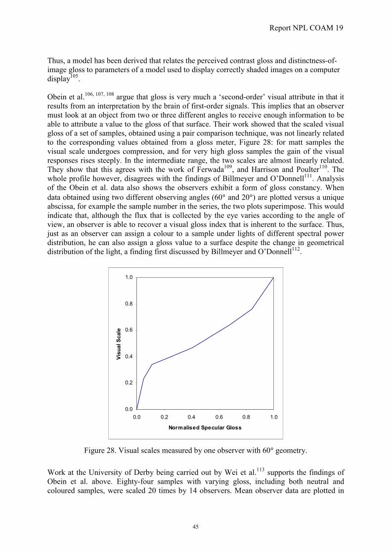
Report NPL COAM 19

45

Thus, a model has been derived that relates the perceived contrast gloss and distinctness-of-image gloss to parameters of a model used to display correctly shaded images on a computer display105. Obein et al.106, 107, 108 argue that gloss is very much a ‘second-order’ visual attribute in that it results from an interpretation by the brain of first-order signals. This implies that an observer must look at an object from two or three different angles to receive enough information to be able to attribute a value to the gloss of that surface. Their work showed that the scaled visual gloss of a set of samples, obtained using a pair comparison technique, was not linearly related to the corresponding values obtained from a gloss meter, Figure 28: for matt samples the visual scale undergoes compression, and for very high gloss samples the gain of the visual responses rises steeply. In the intermediate range, the two scales are almost linearly related. They show that this agrees with the work of Ferwada109, and Harrison and Poulter110. The whole profile however, disagrees with the findings of Billmeyer and O’Donnell111. Analysis of the Obein et al. data also shows the observers exhibit a form of gloss constancy. When data obtained using two different observing angles (60� and 20�) are plotted versus a unique abscissa, for example the sample number in the series, the two plots superimpose. This would indicate that, although the flux that is collected by the eye varies according to the angle of view, an observer is able to recover a visual gloss index that is inherent to the surface. Thus, just as an observer can assign a colour to a sample under lights of different spectral power distribution, he can also assign a gloss value to a surface despite the change in geometrical distribution of the light, a finding first discussed by Billmeyer and O’Donnell112.

0.0

0.2

0.4

0.6

0.8

1.0

0.0 0.2 0.4 0.6 0.8 1.0

Normalised Specular Gloss

Visu

al S

cale

Figure 28. Visual scales measured by one observer with 60� geometry.

Work at the University of Derby being carried out by Wei et al.113 supports the findings of Obein et al. above. Eighty-four samples with varying gloss, including both neutral and coloured samples, were scaled 20 times by 14 observers. Mean observer data are plotted in

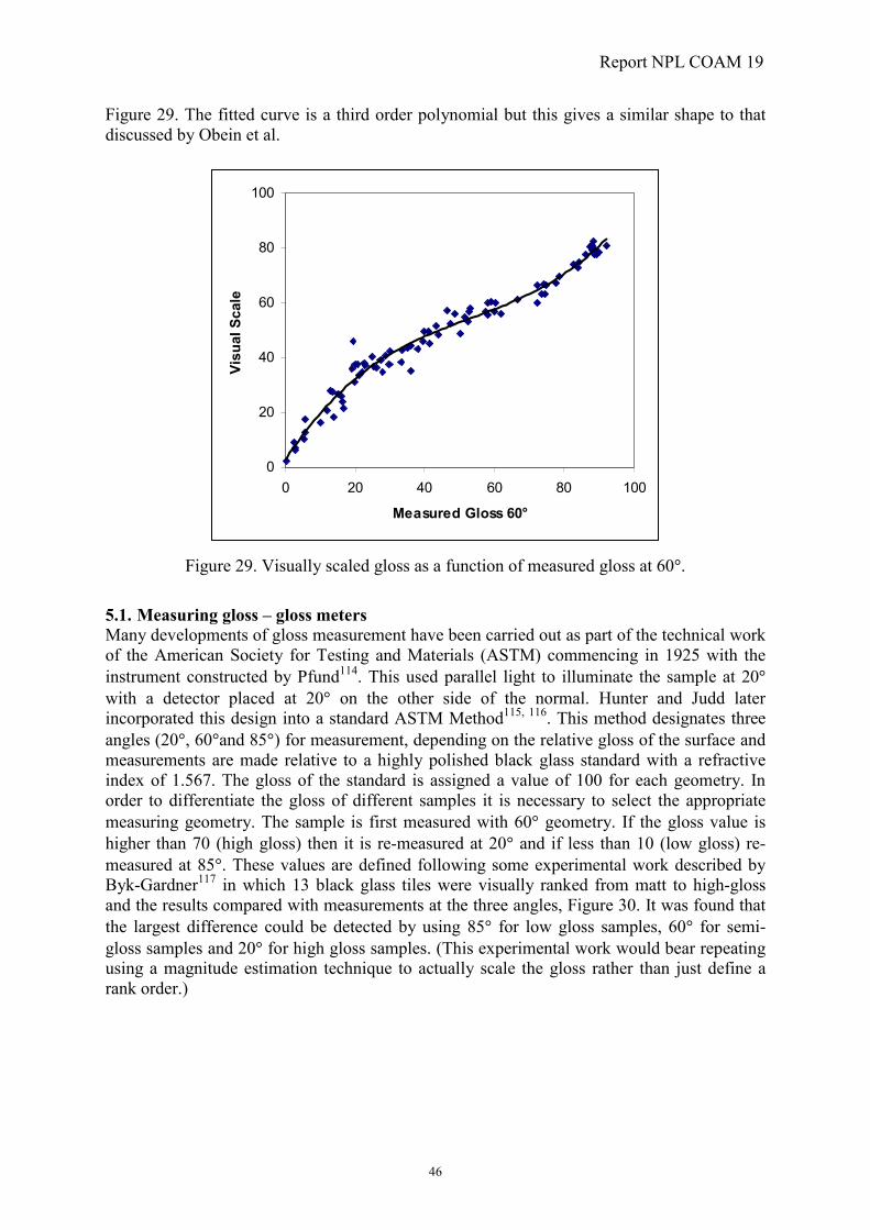
Report NPL COAM 19

46

Figure 29. The fitted curve is a third order polynomial but this gives a similar shape to that discussed by Obein et al.

0

20

40

60

80

100

0 20 40 60 80 100

Measured Gloss 60°

Visu

al S

cale

Figure 29. Visually scaled gloss as a function of measured gloss at 60�.

5.1. Measuring gloss – gloss meters Many developments of gloss measurement have been carried out as part of the technical work of the American Society for Testing and Materials (ASTM) commencing in 1925 with the instrument constructed by Pfund114. This used parallel light to illuminate the sample at 20� with a detector placed at 20� on the other side of the normal. Hunter and Judd later incorporated this design into a standard ASTM Method115, 116. This method designates three angles (20�, 60�and 85�) for measurement, depending on the relative gloss of the surface and measurements are made relative to a highly polished black glass standard with a refractive index of 1.567. The gloss of the standard is assigned a value of 100 for each geometry. In order to differentiate the gloss of different samples it is necessary to select the appropriate measuring geometry. The sample is first measured with 60� geometry. If the gloss value is higher than 70 (high gloss) then it is re-measured at 20� and if less than 10 (low gloss) re-measured at 85�. These values are defined following some experimental work described by Byk-Gardner117 in which 13 black glass tiles were visually ranked from matt to high-gloss and the results compared with measurements at the three angles, Figure 30. It was found that the largest difference could be detected by using 85� for low gloss samples, 60� for semi-gloss samples and 20� for high gloss samples. (This experimental work would bear repeating using a magnitude estimation technique to actually scale the gloss rather than just define a rank order.)

Report NPL COAM 19

47

0

10

20

30

40

50

60

70

80

90

100

1 2 3 4 5 6 7 8 9 10 11 12 13

Visual Assessment

Mea

sure

d Va

lue

20 deg

60 deg

85 deg

Low gloss Semi gloss High gloss

Figure 30. Measurements of a series of samples, at three angles, as a function of visual assessment of their gloss.

Recent work at the Graphic Technology Research Association in Germany (FOGRA) describes experiments to re-assess the measurement of gloss118. It is argued that the current methods for measuring gloss are only valid when comparison is required between surfaces that are nominally similar in visual gloss. In the graphic arts world however, it is required to compare the gloss of unprinted paper with that of printed paper where there can be a considerable perceptual gloss difference. The results of visual experiments suggested that only one angle need be used for measuring gloss, and that the brightness (lightness) of the sample be taken into consideration. It is also suggested that different colours may give different gloss values when printed on the same paper. This difference is partially accounted for however, by taking the relative brightness (lightness) into consideration. The gloss of textile materials, better known as lustre, has been quantified in several ways by different workers but none of the methods has been standardised. Some work supporting the Hunter definition is described by Joshi et al.119. Connected with the above work, ISO TC 130/WG4 Graphic technology/media and materials is leading a series of experiments with the aim of producing a new measure of visual lustre. This measure is based on the ratio of the diffuse reflectance to the specular reflectance with the illumination is set at 45� and visual data for a number samples have been obtained from groups in Germany, Japan, Switzerland and the UK. The samples include a number of different paper types unprinted and printed with cyan, magenta, yellow and black ink. There are potential problems in that the measurements obtained by the different countries, using different instruments, are not all correlated, and the visual experiments differ in detail in the different countries. Further analysis of the data is awaited. A committee draft standard120 is available which proposes the following measure of visual lustre, L, in terms of the specular reflectance with illumination at 45�, I45/45, and the diffuse reflectance, I0/45.

Report NPL COAM 19

48

��

���

� ��

NkII

LogL // 450454599150

where k represents the ratio of measurements made using a reference white:

W/

/

IIk ��

�

����

��

450

4545

and N represents the difference in the measurements made using a black glass:

� �G// kIIN 4504545 �� Early indications however, are that including the diffuse reflectance in the formula does not improve the correlation between the visual data and the measurements121. ISO/IEC JTC1/SC28 Office Equipment, is responsible for developing office equipment standards in the areas of: copying machines; page printers; word processors; electronic typewriters; facsimile equipment; office equipment supplies; office equipment specification sheets; and scanners. The technical committee includes a working group addressing issues to do with the assessment of the printed image quality; included under this heading is gloss, within-page gloss uniformity and page-to-page gloss uniformity, all applied to both black-and-white and colour images of text and/or pictures122. Also introduced is the concept of micro-gloss, to represent the fine structure in the perceived gloss. The presence of this structure can be objectionable and detracts from the overall image quality123, 124, 125, 126. 5.2. Measuring gloss – goniophotometers The most informative and precise technique for measurement of the gloss of surfaces is undoubtedly goniophotometry – the measurement of the intensity of reflected light as a function of viewing angle127. It is often the case that the angle of illumination of a goniophotometer is also variable. Typical goniophotometric data obtained using this type of instrument are shown in Figure 31 where the relative amount of light reflected from a white gloss tile when illuminated with a parallel beam of incident at 8� to the surface normal. The gap in the data, to the left of the figure, indicates the position of the illuminating beam; the gloss peak is shown to the right of the figure. Similar measurements made using a matt tile would show only a small gloss peak – for a perfect matt sample there would be no gloss peak.

Report NPL COAM 19

49

0.000

0.010

0.020

0.030

0.040

-0.020 -0.010 0.000 0.010 0.020

Gloss tileMatt tile

0.01

0.10

1.00

10.00

100.00

1000.00

-90 -75 -60 -45 -30 -15 0 15 30 45 60 75 90

Viewing angle

Log

rela

tive

refle

ctan

ce

Gloss tile

Matt tile

Figure 31. Goniophotometric data plots showing the relative amount of light reflected from a

white gloss tile and a white matt tile over the angular range �85�, when illuminated with a parallel beam of light incident at 8� to the surface normal. Plotted using (a) Cartesian coordinates and (b) polar coordinates – and the logarithm of the relative reflectance.

It is apparent that, if several samples are to be compared, some method must be devised for simplifying the information. The simplest value to consider is the peak height, Is, for a given value of illumination angle, but it has been found that this does not give a significantly better correlation with subjective assessment than does a simple measurement from a gloss meter. One useful way of summarising the information from data for various angles of illumination is shown in Figure 32 in which values of (Is – Id) are plotted against (90� - angle of illumination) for each angle of illumination, where Id is the diffuse reflectance, the intensity

(a)

(b)

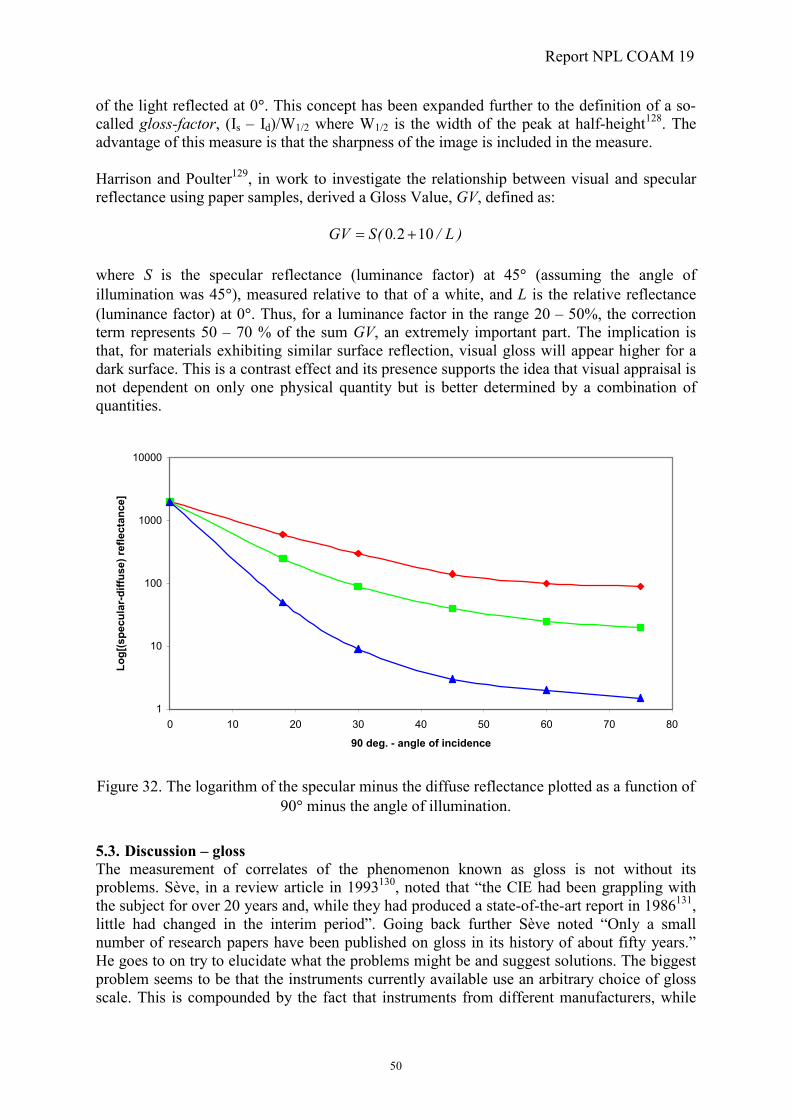
Report NPL COAM 19

50

of the light reflected at 0�. This concept has been expanded further to the definition of a so-called gloss-factor, (Is – Id)/W1/2 where W1/2 is the width of the peak at half-height128. The advantage of this measure is that the sharpness of the image is included in the measure. Harrison and Poulter129, in work to investigate the relationship between visual and specular reflectance using paper samples, derived a Gloss Value, GV, defined as:

)L/.(SGV 1020 �� where S is the specular reflectance (luminance factor) at 45� (assuming the angle of illumination was 45�), measured relative to that of a white, and L is the relative reflectance (luminance factor) at 0�. Thus, for a luminance factor in the range 20 – 50%, the correction term represents 50 – 70 % of the sum GV, an extremely important part. The implication is that, for materials exhibiting similar surface reflection, visual gloss will appear higher for a dark surface. This is a contrast effect and its presence supports the idea that visual appraisal is not dependent on only one physical quantity but is better determined by a combination of quantities.

1

10

100

1000

10000

0 10 20 30 40 50 60 70 80

90 deg. - angle of incidence

Log[

(spe

cula

r-di

ffuse

) ref

lect

ance

]

Figure 32. The logarithm of the specular minus the diffuse reflectance plotted as a function of

90� minus the angle of illumination.

5.3. Discussion – gloss The measurement of correlates of the phenomenon known as gloss is not without its problems. Sève, in a review article in 1993130, noted that “the CIE had been grappling with the subject for over 20 years and, while they had produced a state-of-the-art report in 1986131, little had changed in the interim period”. Going back further Sève noted “Only a small number of research papers have been published on gloss in its history of about fifty years.” He goes to on try to elucidate what the problems might be and suggest solutions. The biggest problem seems to be that the instruments currently available use an arbitrary choice of gloss scale. This is compounded by the fact that instruments from different manufacturers, while

Report NPL COAM 19

51

making measurements at nominally the same angles, show wide variation in the aperture size and beam geometry. Sève proposes that the measurement of gloss be related to the measurement of luminance factor in the specular direction; he also discusses the influence of polarisation on the measurements.

Report NPL COAM 19

52

6. TRANSLUCENCY A translucent material is one that transmits, reflects and scatters light and as a phenomenon, translucency occurs between the extremes of complete transparency and complete opacity. Within the concept of total appearance, translucency has an important part to play because a object may ‘appear’ different depending not just on its colour, but also on the appearance of that colour due to the relationship between the light transmitted, the light reflected, and the light scattered by the body of the object. In order to understand the relationship, for example, between the structure of many food products and the consumer perception of quality, it has been found necessary to understand the part played by translucency132. If it is possible to see an object or scene through a material then that material is said to be transparent. If is it is possible to see only a ‘blurred’ image through the material then it has a degree of transparency the extent of which is a property of the particular material133, 134. This blurring, or loss of information, is due to the diffusion of light as it passes through the material. If it is obvious that no light is being transmitted by the material then it is said to be opaque and opacity can be considered a property of the material whereby the passage of light is inhibited, i.e. the opposite of transparency. Other terms used to describe similar visual effects include clarity, defined in terms of the ability to perceive the fine detail of images through the material; haze, defined as a property of the material whereby objects viewed through it appear to be reduced in contrast; and translucency, a property of the material by which it transmits light diffusely without permitting a clear view of objects beyond it. These terms all imply a scattering or diffusing mechanism within the material but there is an important distinction between clarity and haze. Consider a target that consists of a series of sets of black and white bars and each set is of a different spatial frequency135. For a material with a high value of clarity and a low value of haze, it will be possible to discern a high spatial frequency pattern irrespective of the contrast between the black and the white bars at the highest discernible frequency. For a material with a high value of haze but low value of clarity it will be possible to distinguish only a blurred image at the higher frequencies, because the contrast between the black and white bars appears much reduced. Thus, the concept of translucency can perhaps be regarded as a descriptor of the combined effects defined above as clarity and haze. This implies that it is a more general term and, perhaps, should be limited to use as a subjective term, keeping clarity and haze as descriptors of objective, or measurable, correlates. Also of importance is turbidity which is defined as the reduction in transparency due to the presence of particulate matter in the material. It can be seen from the above discussion that, in general terms, the transparency of the material is determined by the balance between the directly transmitted light and the scattered light; it is the former that conveys information from which the visual sensation, the image, is formed, and the latter which degrades that image. Indeed, it might be thought that the use of the terms translucency, clarity, haze, opacity, etc., is superfluous and that transparency is both totally applicable and sufficient. It has been demonstrated above, however, that there is a clear distinction between the perceived contrast of an image and the detection of fine detail in that image: thus the terms haze and clarity are required. Indeed, it can be demonstrated that a series of materials that lead to a decrease in haze might show increasing clarity.

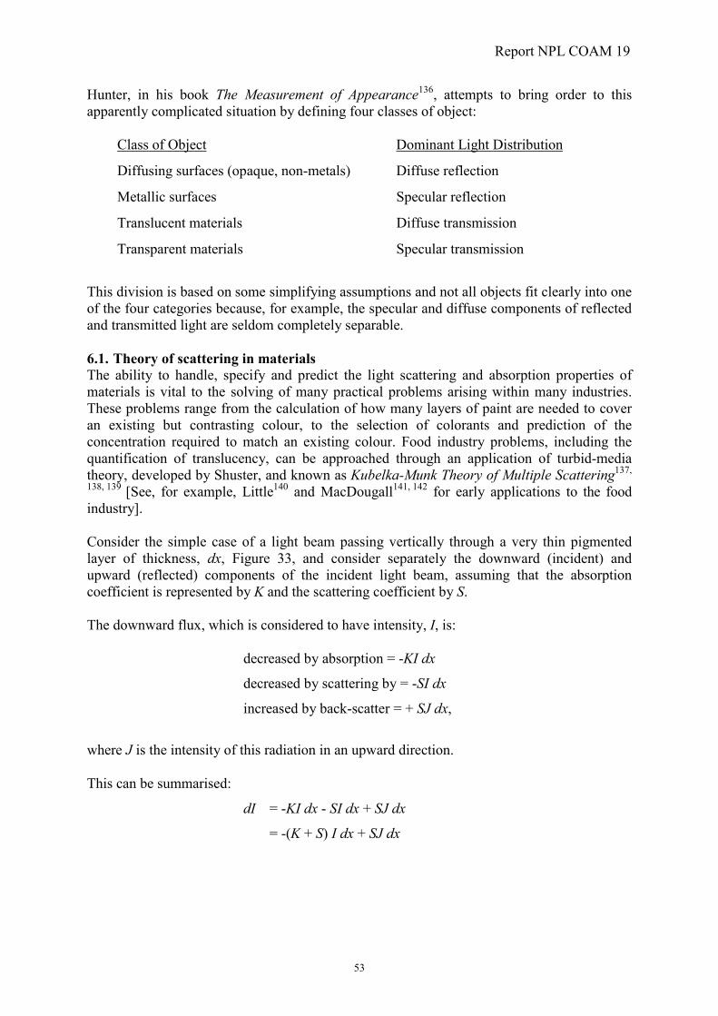
Report NPL COAM 19

53

Hunter, in his book The Measurement of Appearance136, attempts to bring order to this apparently complicated situation by defining four classes of object:

Class of Object Dominant Light Distribution

Diffusing surfaces (opaque, non-metals) Diffuse reflection

Metallic surfaces Specular reflection

Translucent materials Diffuse transmission

Transparent materials Specular transmission

This division is based on some simplifying assumptions and not all objects fit clearly into one of the four categories because, for example, the specular and diffuse components of reflected and transmitted light are seldom completely separable. 6.1. Theory of scattering in materials The ability to handle, specify and predict the light scattering and absorption properties of materials is vital to the solving of many practical problems arising within many industries. These problems range from the calculation of how many layers of paint are needed to cover an existing but contrasting colour, to the selection of colorants and prediction of the concentration required to match an existing colour. Food industry problems, including the quantification of translucency, can be approached through an application of turbid-media theory, developed by Shuster, and known as Kubelka-Munk Theory of Multiple Scattering137,

138, 139 [See, for example, Little140 and MacDougall141, 142 for early applications to the food industry]. Consider the simple case of a light beam passing vertically through a very thin pigmented layer of thickness, dx, Figure 33, and consider separately the downward (incident) and upward (reflected) components of the incident light beam, assuming that the absorption coefficient is represented by K and the scattering coefficient by S. The downward flux, which is considered to have intensity, I, is: decreased by absorption = -KI dx

decreased by scattering by = -SI dx

increased by back-scatter = + SJ dx,

where J is the intensity of this radiation in an upward direction. This can be summarised:

dI = -KI dx - SI dx + SJ dx

= -(K + S) I dx + SJ dx

Report NPL COAM 19

54

Surface of film

x

I

J

dx

Substrate

Figure 33. The simple case of a light beam passing vertically through a very thin pigmented layer of thickness, dx, with a downward component I, and upward component J.

At the same time, the upward flux of intensity, J, is: decreased by absorption = -KJ dx

decreased by scattering by = SJ dx

increased by back-scatter = + SI dx,

where I is the intensity of this radiation downwards as above: dJ = -KJ dx - SJ dx + SI dx

= -(K + S) J dx + SI dx

The solution to these differential equations depends on the boundary conditions applied but, in the absence of scattering (S = 0), leads to the familiar Lambert-Bouguer Law for the downward flux:

)Kl(expII �� 0 i.e. layers of equal thickness, l, of the same material transmit the same fraction of the incident monochromatic radiation, I/I0, whatever its intensity: K is known as the absorption coefficient. For an isotropically absorbing and scattering layer of infinite thickness, or at least so thick that the background layer reflection can be considered negligible, it leads to the widely used Kubelka-Munk expression:

�

��

�

R)R(S/K

21 2

where R� = Jo/Io is the reflection factor at the surface for a sample of infinite thickness.

Report NPL COAM 19

55

A number of other solutions for the above differential equations have been tabulated by Judd and Wyszecki143 and a more complete discussion of Kubelka-Munk theory can be found in Nobbs144. Of interest are those that relate the reflectance, R, of a colorant layer backed by a known reflectance, Rg, where Ro is the reflectance of a layer with an ideal black background, i.e. Rg = 0, and those that relate the internal transmittance, Ti, of the layer and its reflectance properties:

KKS

RRRRR

Rag

g ��

��

�

�

��

�

� ���

0

0

21

baR ��

�

where 22 1)a(b ��

220

2 b)Ra(Ti ���

Thus two measurements of a thin layer of a sample, over a white and a black background, enable K and S to be calculated. Some of the major limitations of the Kubelka-Munk type of analysis are that it deals only with monochromatic radiation, and handles only two fluxes (diffuse light travelling upwards or downwards) through a homogenous absorbing and scattering medium. The light loss through the edges is neglected, as are the reflections from the front surface of the sample and the diffuse light incident upon this surface from the inside. It is possible to apply a correction for this latter effect145. Coffee is a convenient model system for demonstrating the effect of translucency properties and the use of K/S measurements146, 147. In an experiment148, nine samples, differing in amount of coffee and whitener concentration, were presented to observers in vertical sided, glazed white, cups and assessed for creaminess and strength. Thin layers were assessed for opacity. It was found that these three attributes could be defined in terms of the K/S ratio and the internal transmittance, Ti, Figure 34.

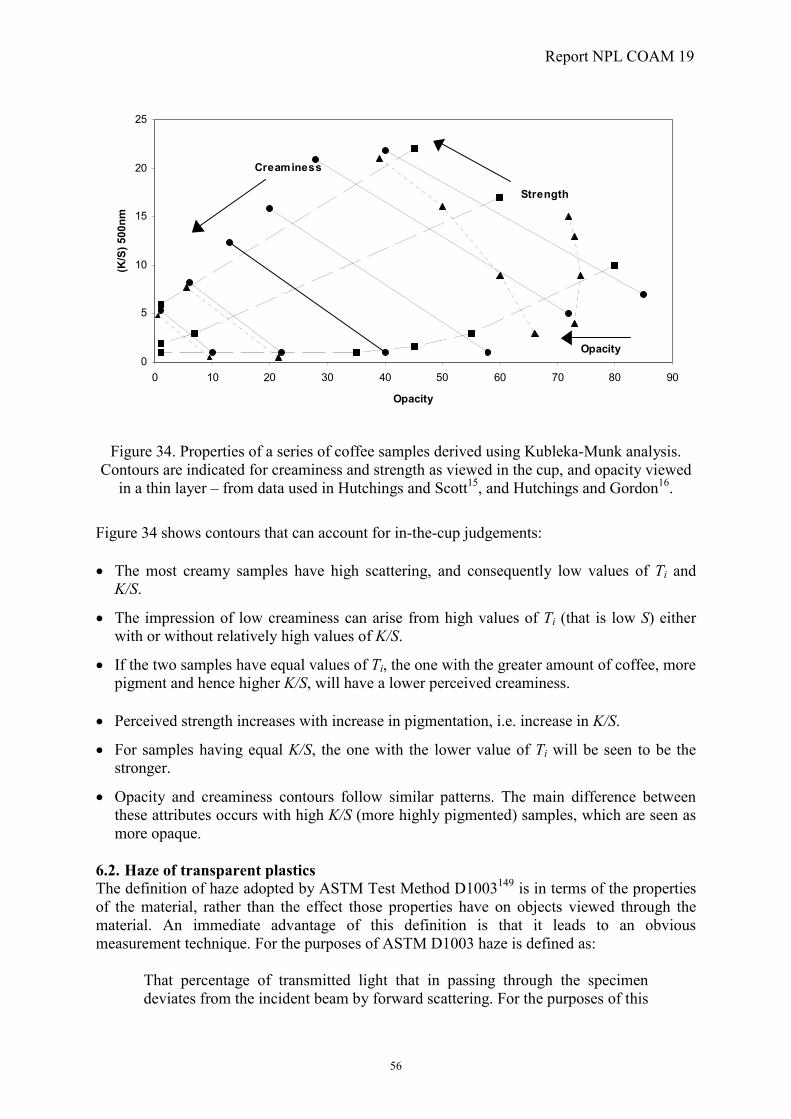
Report NPL COAM 19

56

0

5

10

15

20

25

0 10 20 30 40 50 60 70 80 90

Opacity

(K/S

) 500

nm

Strength

Creaminess

Opacity

Figure 34. Properties of a series of coffee samples derived using Kubleka-Munk analysis. Contours are indicated for creaminess and strength as viewed in the cup, and opacity viewed

in a thin layer – from data used in Hutchings and Scott15, and Hutchings and Gordon16.

Figure 34 shows contours that can account for in-the-cup judgements: �� The most creamy samples have high scattering, and consequently low values of Ti and

K/S.

�� The impression of low creaminess can arise from high values of Ti (that is low S) either with or without relatively high values of K/S.

�� If the two samples have equal values of Ti, the one with the greater amount of coffee, more pigment and hence higher K/S, will have a lower perceived creaminess.

�� Perceived strength increases with increase in pigmentation, i.e. increase in K/S.

�� For samples having equal K/S, the one with the lower value of Ti will be seen to be the stronger.

�� Opacity and creaminess contours follow similar patterns. The main difference between these attributes occurs with high K/S (more highly pigmented) samples, which are seen as more opaque.

6.2. Haze of transparent plastics The definition of haze adopted by ASTM Test Method D1003149 is in terms of the properties of the material, rather than the effect those properties have on objects viewed through the material. An immediate advantage of this definition is that it leads to an obvious measurement technique. For the purposes of ASTM D1003 haze is defined as:

That percentage of transmitted light that in passing through the specimen deviates from the incident beam by forward scattering. For the purposes of this

Report NPL COAM 19

57

method only the light flux deviating more than 2.5 degrees (0.044 rad.) on the average is considered to be haze.

It is necessary to translate this definition into a suitable instrumental technique and the ASTM Method describes a suitable device150. Four measurements are needed: the incident light, T1, with no specimen and a white standard on the sphere port; the total light transmitted by specimen, T2, with the sample in place and a white standard on the sphere port; the light scattered by instrument, T3, with no specimen and a light trap on the sphere port; and the light scattered by the instrument and the specimen T4, with the specimen in place and a light trap on the sphere port. Although not strictly necessary, it is usual to calculate the total luminous transmittance of the specimen, Tt, as well as the haze, H. The equations used are:

%x)T/T(Tt 10012�

%x)]T/T()T/T[(H 1001324 ��

Note that if the diffuse transmittance, Td, is defined by:

11234 T/)]T/T(TT[Td �� then the haze, H, can be defined by:

%xT/TH td 1004� The spectral and geometric requirements detailed in the Standard are precise and must be adhered to in order that comparative measurements can be made. A series of calibrated haze standards is needed for periodic verification of the accuracy and precision of the measurements obtained using the instrument. Ideally, these standards should be suitable thicknesses of a material similar to that usually measured. BS EN ISO 13468, Determination of the Total Luminous Transmittance of Transparent Materials, 1996151 follows the methodology described for ASTN D1003 above. 6.3. A new instrument Dia-Stron Limited, of Andover, have been developing an instrument to measure the light back-scattered by a ‘translucent’ material. This instrument is based on the principles outlined in a patent152 and the main use of the instrument, as described in this patent, is to measure the scattering properties of skin153, 154. This measurement must be made non-invasively in order that the instrument does not influence the parameters it is trying to measure. The particular interests of Dia-Stron however, are in the measurement of the translucency of liquids and their method is particularly applicable to relatively opaque materials. Thus, on a scale of translucency going from transparent to opaque, Dia-Stron are operating at the relatively high opacity, or low transparency, end.

Report NPL COAM 19

58

Incident light Photodetector arrayon top of a fibre-optic faceplate

Scattering medium

Figure 35. Principle of the Dia-Stron instrument

A pulse of light enters the material and is scattered, Figure 35. Adjacent to the light source, a light-emitting diode (LED), is a linear photo-diode array that detects the light back-scattered by the medium. The front surface of this array is fitted with a fibre-optic light-guide to ensure that only light approximately normal to the surface is detected. It can be shown, Figure 36, that this light level, as a function of distance from the source, is a characteristic of the scattering properties of the material155. It is assumed that the thickness of the scattering medium is such that no light is transmitted. Based on this assumption, the method might not be suitable when applied to materials that have a relatively high transparency because a large path length would be required to satisfy this criterion.

-25

-20

-15

-10

-5

0

0 20 40 60 80 100

Detection distance r mm

Mea

sure

d va

lue

ln(r

)

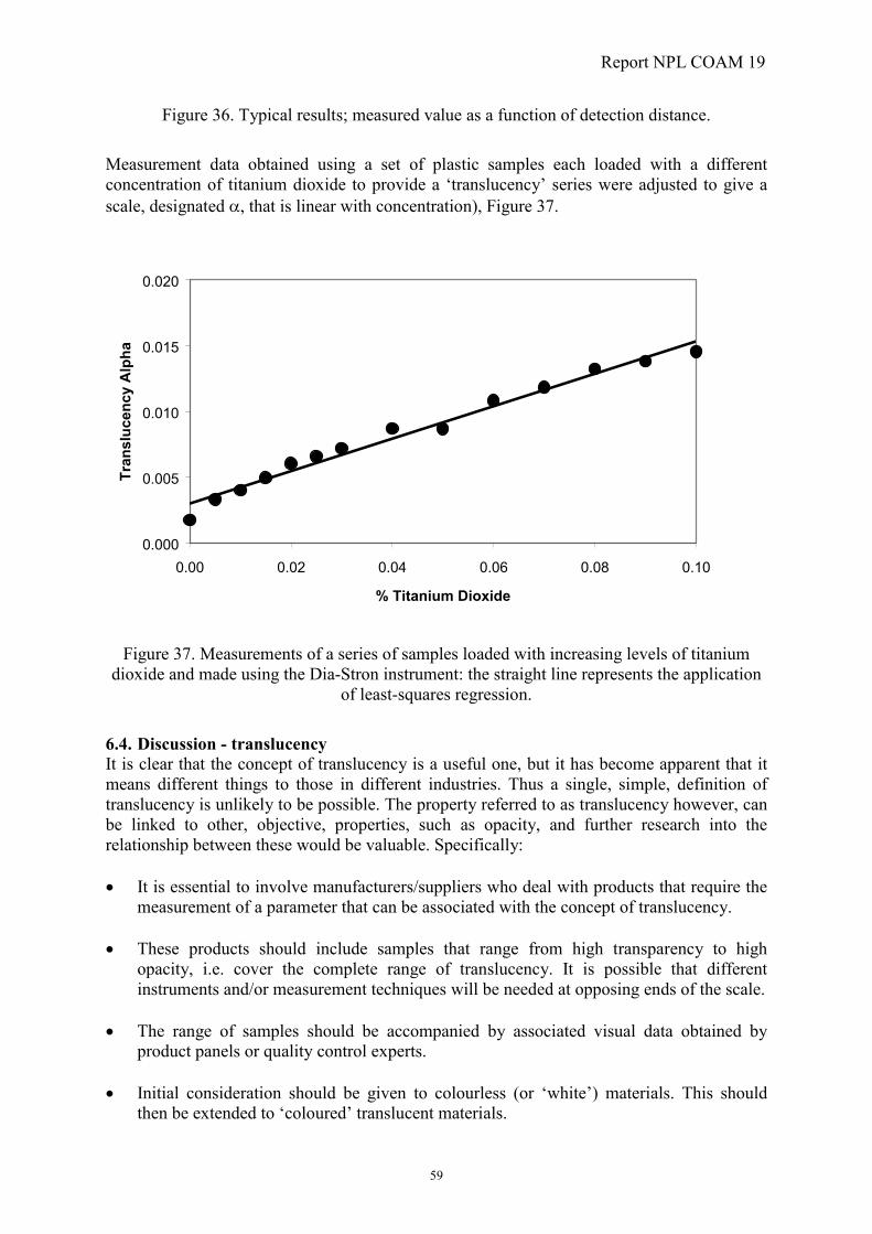
Report NPL COAM 19

59

Figure 36. Typical results; measured value as a function of detection distance.

Measurement data obtained using a set of plastic samples each loaded with a different concentration of titanium dioxide to provide a ‘translucency’ series were adjusted to give a scale, designated , that is linear with concentration), Figure 37.

0.000

0.005

0.010

0.015

0.020

0.00 0.02 0.04 0.06 0.08 0.10

% Titanium Dioxide

Tran

sluc

ency

Alp

ha

Figure 37. Measurements of a series of samples loaded with increasing levels of titanium dioxide and made using the Dia-Stron instrument: the straight line represents the application

of least-squares regression.

6.4. Discussion - translucency It is clear that the concept of translucency is a useful one, but it has become apparent that it means different things to those in different industries. Thus a single, simple, definition of translucency is unlikely to be possible. The property referred to as translucency however, can be linked to other, objective, properties, such as opacity, and further research into the relationship between these would be valuable. Specifically: �� It is essential to involve manufacturers/suppliers who deal with products that require the

measurement of a parameter that can be associated with the concept of translucency. �� These products should include samples that range from high transparency to high

opacity, i.e. cover the complete range of translucency. It is possible that different instruments and/or measurement techniques will be needed at opposing ends of the scale.

�� The range of samples should be accompanied by associated visual data obtained by

product panels or quality control experts. �� Initial consideration should be given to colourless (or ‘white’) materials. This should

then be extended to ‘coloured’ translucent materials.

Report NPL COAM 19

60

�� It would be constructive to carry out a simple visual experiment, based on a series of

plastic samples of varying translucency, to demonstrate the difference between the concepts of clarity and haze.

�� Future ‘translucency’ standards will probably have to be related to specific industrial

needs: a series of plastic samples with varying loading of titanium dioxide could be a useful starting point.

Report NPL COAM 19

61

7. SURFACE TEXTURE The fourth aspect of appearance assessment to be considered is that of surface texture, Figure 9. The concept of texture is intuitively obvious but is difficult to define. ASTM156 has:

The visible surface structure depending on the size and organisation of small constituent parts of a material; typically, the surface of a woven fabric.

While this definition is satisfactory, it is by no means complete and is, perhaps, spoilt by the example. If this is a definition of surface texture, it is necessary to differentiate between what is becoming known as physical texture, texture associated with physical, topological, variability in a surface, and optical texture, texture associated with spatial variation in appearance caused by non-uniformity of colorant, Figure 37. Example of the former are the woven fabric and the surface of a metal, and of the latter is a metallic automobile finish where the variation caused by the spatial distribution of the discrete aluminium flakes is visible through an acrylic varnish overcoat which itself gives a smooth, high gloss, finish. In the past, surface texture has been assessed by the judgement of an inspector, either by eye or even by fingernail. In order to put a number to the surface texture, a more accurate means of measurement is required. A typical surface-measuring instrument will consist of a stylus with a small tip (the fingernail), a gauge or transducer, a traverse datum and a processor. The surface is measured by moving the stylus across the surface. As the stylus moves up and down along the surface, the transducer converts this movement into a signal which is then exported to a processor which converts this into a number and usually a visual profile157. For correct data collection, the gauge needs to pass over the surface in a straight line such that only the stylus tip follows the surface under test. This is done using a straightness datum. This can consist of some form of datum bar that is usually lapped or precision ground to a high straightness tolerance. Two attributes are distinguished: roughness, and waviness. Roughness is a measure of the process marks produced during the creation of the surface and other factors such as the structure of the material, and waviness is a longer wavelength variation in surface away from its basic form158, 159, 160. The human response to texture can be using terms like fine, coarse, grained, smooth. Alternatively, texture can be described as a variation in tone (intensity or lightness161) and structure. Other responses to a physical surface may be in terms of its roughness, smoothness, ripple or orange peel, or its apparent mottle or speckle. Whichever scheme is used the words are attempting to describe a variation and it is pertinent to try to establish what it is that is actually varying. The building blocks of texture can be considered as texture elements – those elements of the physical surface that are perceived to be different162. These have variously been called texture primitives, texture elements, textons and texels. Texture can then be described by the number and types of primitives, and by their relative spatial relationships, a process called texture classification. It should also be noted that the perception of physical texture is scale dependent; the viewing distance from the physical surface will influence the perception: it is also dependent on the angles of illumination and viewing163.

Report NPL COAM 19

62

. . . . .

. . . . .

. . . . .

(a)

(b)

(c)

Figure 38. (a) Texture primitive; (b) Pattern generated by a line of primitives; (c)2-dimensional texture pattern generated by an array of lines of primitives.

Consider a texture primitive, a circle, Figure 38(a), that builds up into a line a circles, (b), and then an array of circles (c). This simple example shows the formation of a (regular) textured pattern based on the simple texture primitive, a circle. If this formation process could be reversed, and applied to more complex patterns (textures), to define the primitive and its spatial repeat, then a suitable analysis technique, texture segmentation, has been devised. If texture is considered as a variation along a linear dimension of a material, then there are a number of techniques that can be used to provide numbers that relate to this variation. By including the analysis of several, parallel, lines then a spatial map can be built up. The advent of digital image processing techniques, based on the output from digital cameras, for example, has led to the easy availability of data to enable this process to be carried out and has, indeed, led to techniques that analyse the complete image data in a direct spatial sense. This, in turn, has led to the published literature concerned with texture analysis being very prolific. There are applications, based on digital imaging, in the military (target recognition in camouflage situations, and terrain classification from aerial images), in machine vision (product detection during manufacture to find inadequate mixing in biscuits or other defects in the product), and in the medical world (for remote diagnosis and radiographic image interpretation). In these applications, it is sometimes possible to compare a sample image with a ‘standard’ image but in many circumstances, it is necessary to analyse the spatial distributions in the actual image to detect the required perturbation. It should be noted that, in some applications, it is the detection of objects in the image that is important (pattern recognition); in other applications, it is an analysis of the noise pattern that requires an understanding of the texture (texture segmentation). 7.1. Psychophysics One reason why it is important to study the psychophysics of texture perception is that the performance of various texture algorithms is evaluated against the performance the human

Report NPL COAM 19

63

visual system doing the same task164. Julesz has studied texture perception extensively in the context of texture discrimination165, 166, 167. The question he posed was “When is a texture pair discriminable, given that they have the same brightness, contrast and colour?” Julesz concentrates on the spatial statistics of the image grey levels that are inherent in the definition of texture by keeping other illumination-related properties the same. The results of the experiments suggested that two textures are not discriminable if their second-order statistics are identical. (First-order statistics are to do with the likelihood of observing a specific pixel value at a random position in an image, second-order statistics are defined as the likelihood of observing a pair of pixel values at two defined locations in the image.) Thus, Julesz favours an explanation of texture discrimination in terms of spatial distribution. Beck et al.168, however, argue that the perception of texture is primarily a function of spatial frequency and not the result of grouping of spatial information. 7.2. Illumination Chantler argues that the appearance of surface texture is dependant on the direction and angle of the illumination169, 170. Thus, many researchers recognise that the texture appears different when viewed from different directions but do not consider that the texture will also appear different when viewed from a fixed direction but under variable direction and angle of illumination. Chantler shows that the use of directed illumination during image capture, can act as a directional filter of texture, and that the directional characteristics of the texture are not just a function of surface relief but are affected by the angle of the illumination. Chantler further shows that the use of the analysis of stereo pairs, with their associated differences in illumination and view-point, gives advantages in surface texture classification171. 7.3. Analysis techniques Overall, texture analysis can be considered under two headings: syntactic and analytical, Figure 39. The latter is essentially subjective and, as discussed above, there are, as yet, no common perceptual scales that can be assigned to such an analysis172. On the other hand, digital images can be thought of as arrays of data representing the spatial world and, as such, they lend themselves to computational analysis and a number of techniques have been proved useful.

Report NPL COAM 19

64

TEXTURE

Optical Physical

Syntactic Analytical

Fine, coarse

Tone: light, dark

Rough, smooth, rippled

Matte, speckled

Regular, irregular

Structural

Statistical

Spectral

Fractal

Figure 39. Texture analysis via analytical and syntactic routes.

Those methods described in the literature are called by different names by different authors but they can loosely be discussed under two headings, Figure 39:

�� structural – where the texture is considered to be defined by sub-patterns, called primitives (examples are those methods based on autocorrelation and spatial frequency analysis);

�� statistical – where the texture is defined by a set of statistics extracted from the entire textural region (examples are methods based on co-occurrence matrices or on run length)

The different methods capture the inherent coarseness or fineness of texture173, 174, 175. Fractal based texture classification is another approach that attempts to find correlation between texture coarseness and fractal dimension. 7.4. Autocorrelation Assuming that the variation causing the perception of texture can be measured in some way (by a trace of profile height if physical, or by the digital values from an electronically derived image), then the standard deviation about the mean value of this parameter can be used to describe the amplitude characteristics of the variation. A much more informative approach to this analysis, however, is to use methods routinely used in communications theory. Instead of just evaluating the mean square of the values associated with each pixel, the mean of the product of these values and those separated by a defined distance is calculated. The result, a plot of the product versus the distance, is known as the autocorrelation function of the texture and is a measure of the dependence of a series of values at one point on the values at another

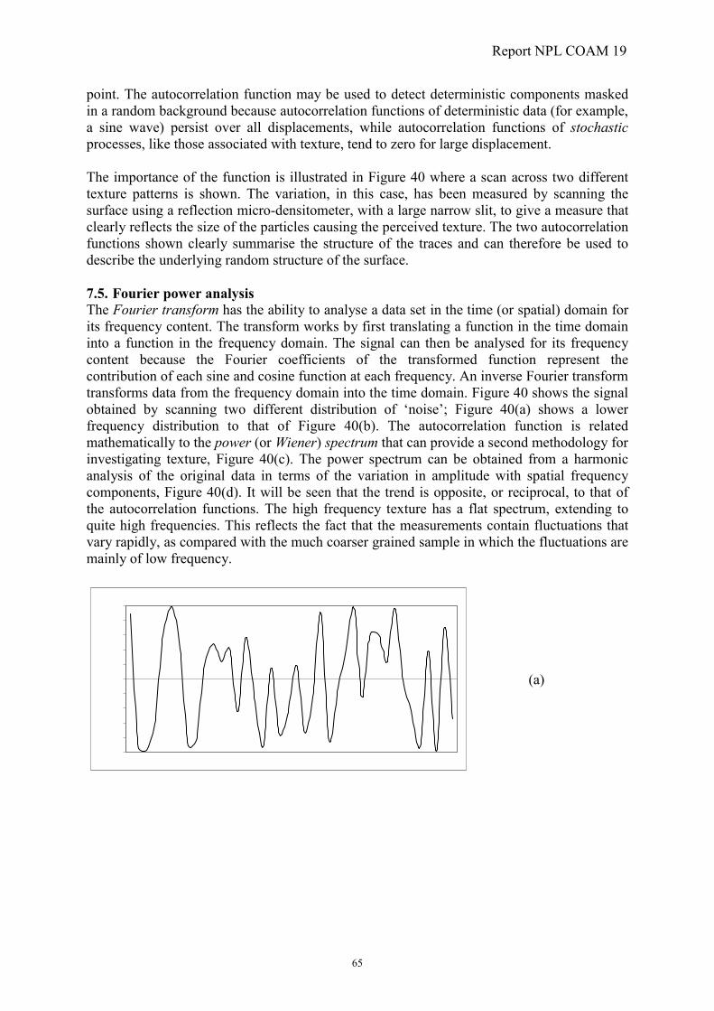
Report NPL COAM 19

65

point. The autocorrelation function may be used to detect deterministic components masked in a random background because autocorrelation functions of deterministic data (for example, a sine wave) persist over all displacements, while autocorrelation functions of stochastic processes, like those associated with texture, tend to zero for large displacement. The importance of the function is illustrated in Figure 40 where a scan across two different texture patterns is shown. The variation, in this case, has been measured by scanning the surface using a reflection micro-densitometer, with a large narrow slit, to give a measure that clearly reflects the size of the particles causing the perceived texture. The two autocorrelation functions shown clearly summarise the structure of the traces and can therefore be used to describe the underlying random structure of the surface. 7.5. Fourier power analysis The Fourier transform has the ability to analyse a data set in the time (or spatial) domain for its frequency content. The transform works by first translating a function in the time domain into a function in the frequency domain. The signal can then be analysed for its frequency content because the Fourier coefficients of the transformed function represent the contribution of each sine and cosine function at each frequency. An inverse Fourier transform transforms data from the frequency domain into the time domain. Figure 40 shows the signal obtained by scanning two different distribution of ‘noise’; Figure 40(a) shows a lower frequency distribution to that of Figure 40(b). The autocorrelation function is related mathematically to the power (or Wiener) spectrum that can provide a second methodology for investigating texture, Figure 40(c). The power spectrum can be obtained from a harmonic analysis of the original data in terms of the variation in amplitude with spatial frequency components, Figure 40(d). It will be seen that the trend is opposite, or reciprocal, to that of the autocorrelation functions. The high frequency texture has a flat spectrum, extending to quite high frequencies. This reflects the fact that the measurements contain fluctuations that vary rapidly, as compared with the much coarser grained sample in which the fluctuations are mainly of low frequency.

-0.5-0.4-0.3-0.2-0.10.00.10.20.30.40.5

1

(a)

Report NPL COAM 19

66

-0.5-0.4-0.3-0.2-0.10.00.10.20.30.40.50.6

1

0.00.20.40.60.81.01.21.4

0.0 1.0 2.0 3.0 4.0 5.0 6.0 7.0

Distance

0.0

0.2

0.4

0.6

0.8

1.0

1.2

0 50 100 150 200

Spatial frequency (cycles/mm)

Figure 40. Autocorrelation functions (c) and noise-power (Wiener spectra) (d) of two different structures (a) and (b).

The presence of prominent peaks in the frequency spectrum gives the principal direction of the texture patterns; the location of the peaks in the spectrum gives the fundamental spatial period of the patterns; and eliminating the periodic components gives the non-periodic elements, which can then be described by statistical techniques. Although the autocorrelation function and the power spectrum are closely related, and may be readily calculated from each other, they both have distinct roles. The autocorrelation function relates well to the causes of the physical variation while the power spectrum is important in assessing its visual impact.

(b)

(c)

(d)

Report NPL COAM 19

67

7.6. Co-occurrence matrices To move from the structural analysis of texture to a more statistical approach, co-occurrence matrices count how often pairs of neighbouring grey levels of pixels, that are separated by a certain distance and lie along a certain direction, occur in a digital image of the surface texture of a sample. The concept of tone is based on the varying shades of grey in the digital image. This form of analysis makes an inherent assumption that texture is perceived as perturbation in tonal (brightness or, relatively, lightness) information only. An argument to support this statement can be based on the example of a piece of fabric woven from a single coloured thread. Texture is seen in the final product, so is a variation in colour. Because the colour of the constituent thread is constant, however, the perceived spatial variation, the texture, must be due to the regular pattern of the weave and the spatial variation in lightness or tone. Thus, it is reasonable to conduct the analysis using this parameter. A classic paper by Haralick et al. describes the process of generating co-occurrence matrices in detail176, 177. Consider an image of a textured pattern. The image is rectangular and each pixel is quantised to a defined number of levels: in most PC based analysis systems, this number of levels will be 256 (28) representing an 8-bit system. In a coloured image, each pixel will have an associated red, green and blue quantised level; in a black-and-white image there will be only one scale, usually described by the grey levels. It is assumed that the texture content information in the image is contained in the overall or ‘average’ spatial relationship that the grey levels have to one another. There are four, closely related, measures from which all of the texture features are derived. These measures are the arrays derived by investigating the values of nearest-neighbour pixels where the pixel separation, d, is equal to 1. In a subset of the image, Figure 41, pixels 1 and 5 are 0� nearest neighbours to the central pixel; pixels 2 and 6 are 135� nearest neighbours; pixels 3 and 7 are 90� nearest neighbours; and pixels 4 and 8 are 45� nearest neighbours. Note that this information is purely spatial and not related to the pixel bit value. The co-occurrence matrix is comprised of the relative frequencies with which two nearest neighbour pixels, separated by a given distance (defined in terms of a number of pixels) occur in the image.

6 87

5 1x

4 23

0 degrees

45 degrees90 degrees135 degrees

Figure 41. Pixels 1 and 5 are 0� (horizontal) nearest neighbours to pixel x; pixels 2 and 6 are 135� nearest neighbours; pixels 3 and 7 are 90� nearest neighbours; and pixels 4 and 8 are 45�

nearest neighbours to x.

Report NPL COAM 19

68

The process is best explained by an example. Consider a 4 by 4 image with three grey-scale values, Figure 42(a) (Haralick, Figure 3). The general form of the grey-scale value spatial dependence matrix for this image is shown in Figure 42(b). Figure 42(c-f) then give matrices, P, containing the number of times, the occurrence, each of the respective pairs of adjacent pixels, for each of the four direction operators. Thus the pair with grey-scale values (0, 0) occurs four times; pixels (1, 1) and (1, 2), pixels (1, 2) and (1, 1), pixels (2, 1) and (2, 2), and pixels (2, 2) and (2, 1). The total number of nearest-neighbour pixel pairs for each operator is as follows:

�� For the 0� operator, and for an image comprising Nx rows and Ny columns, there are a total of 2Ny(Nx – 1) nearest neighbour pixel pairs.

�� For the 45� operator, there will be 2(Nx – 1) neighbouring pixel pairs in all except the first row where there are none, and there are Ny rows. This provides a total of 2(Ny – 1)(Nx – 1) nearest-neighbour pixel pairs.

�� For the 90� operator, by symmetry, there will be 2Nx(Ny-1) pairs.

�� For the 135� operator, by symmetry there will be 2(Nx – 1)(Ny – 1) pairs. It can be seen that, for images comprising many millions of pixels, and quantised to 8-bits, the size of the co-occurrence matrix is very large. The computational complexity is compounded by the fact that co-occurrence may be investigated between pixels where the separation, d, has an integer value greater than unity.

Report NPL COAM 19

69

(0,0) (0,3)(0,2)(0,1)

(1,0) (1,3)(1,2)(1,1)

(2,0) (2,3)(2,2)(2,1)

(3,0) (3,3)(3,2)(3,1)

1 32 4

1

2

4

3

(a)

0 110

2 332

0 222

0 110

(b)

4 012

0 210

1 160

2 004

6 020

0 020

2 222

0 024

4 001

0 010

0 142

1 122

2 031

0 020

3 261

1 012

(c) (d)

(f)(e)

900

1450

00

1350

Figure 42. (a) A 4 x 4 image with four grey scale values 0-3. (b) General form of and grey-scale spatial dependence matrix for an image with grey-scale values 0-3 – the elements (i, j)

stand for the number of times grey-scale values i and j are nearest neighbours. (c)-(f) Calculation of all four distance 1 grey-tone spatial-dependence matrices.

An initial assumption of this technique is that all of the texture information is contained in the grey-scale spatial-dependent matrices. From these matrices, a set of 14 measures of textural features is now defined in Table 4 below.

Report NPL COAM 19

70

Table 4. Classifiers described by Haralick. Classifiers that express visual textual features: f1 – Angular second moment – homogeneity f2 – Contrast f3 – Correlation – grey scale linear dependencies Classifiers that are based on statistics: f4 – Sum of squares f5 – Inverse difference moment f6 – Sum average f7 – Sum variance f10 – Difference variance Classifiers that are based on information theory, in particular entropy: f8 – Sum entropy f9 – Entropy f11 – Difference entropy Classifiers that are based on information measures of correlation: f12 – Information measure of correlation (i) f13 – Information measure of correlation (ii) f14 – Maximal correlation coefficient

Specific equations for each of these attributes are given in the paper178. Note that a moment is a tool for representing the shape of an object, e.g. the centre-of-gravity, or the orientation and the translation from a reference point. Thus, for a chosen value of pixel separation, d, there are four, angular, grey-value spatial-dependency matrices. Hence there are four values of each of the above 14 measures. The mean and range of each of these 14 measures, averaged over the four values, comprise the set of 28 features that can be used as inputs to a texture classifier. Haralick describes early examples of the application of this technique related to the detection of features in satellite images, what might be called macro-texture, and related to the categorisation of various rocks (sandstones) where different types of rock were identified by their texture using (black-and-white) photo-micrographic images; this latter application might be termed micro-texture. Gotlieb179 describe experiments in which textures from the Brodatz book of textures�, together with those from a number of other sources, were analysed. It was found possible to use co-occurrence matrices and derive measures that enabled the various texture patterns to � A standard reference for texture classification has been the 112 images in the album designed for use by graphic artists, Phil Brodatz, Textures: A Photographic Album for Artists and Designers, Dover Publications, New York, 1966.

Report NPL COAM 19

71

classified in a similar manner to that used in the book. Six of the Haralick parameters were found to be particularly useful: f1, f2, f5, f9, f12 and f13. A study into the classification of the texture of the same breakfast cereal, manufactured at several sites throughout the world (with the basic wheat sourced locally) also showed that the Haralick measures were adequate. This latter method was based on coloured images obtained with a one-megapixel digital camera180. 7.7. Run length analysis This method of texture analysis, sometimes called primitive length analysis, bears some resemblance to the concept behind the autocorrelation method in that it looks for patterns along lines in an image of the texture, and some resemblance to the method using co-occurrence matrices181. The method requires the calculation of the number of times a ‘run’, a set of equal identical pixels, occurs in an image, for various run lengths. Analysis can be performed in only one direction but further information can be obtained by carrying the calculations using an additional orthogonal direction. Five measures are defined: �� Short run emphasis – the run length value divided by the square of the length of the run,

normalised by dividing by the total number of runs in the image;

�� Long run emphasis – the run length value multiplied by the square of the length of the run, normalised by dividing by the total number of runs in the image;

�� Grey level non-uniformity – the square of the number of run lengths at each grey value, normalised by dividing by the total number of runs in the image;

�� Run length non-uniformity – the sum of the squares of the number of runs for each length, normalised by dividing by the total number of runs in the image;

�� Run percentage – the ratio of the total number of runs to the total number of possible runs if all runs had a length of one.

Galloway182 describes a successful application of this technique to feature analysis in a set of images and there are several comparative studies published in the literature, including some that do not explicitly use grey level analysis but recognise that the world is coloured and carry out the analysis using a colour digital image. Siew et al.183 have applied this co-occurrence matrix method to an analysis of carpet wear. They found useful correlation between the subjective scaling of physical wear and a number of the statistics that form an output to the process. They also applied run length analysis, again, with useful results. 7.8. Other methods The methods described above are not exhaustive; there are a number of other methods mentioned in the literature that might be applicable to specific circumstances including:

�� Fractal analysis – compares texture coarseness and fractal dimension184, 185, 186, 187.

�� Edge frequency – similar to run length analysis but uses the distance-related gradients of the difference between adjacent pixels rather than the similarity of adjacent pixels. This lead to the detection of edges and the frequency of occurrence of those edges.

�� Law’s Method – use gradient operators (matrices) to ‘filter’ an image to extract features.

�� Mathematical morphology – based on the use of set theory to extract image components such as shape boundaries, texture primitives and the convex hull (Formally: the smallest

Report NPL COAM 19

72

convex set containing the points. Informally: the rubber band wrapped around the "outside" points.

�� Autoregression texture model.

�� Markov random field model – this model assumes that the value of a specific pixel depend only on the values of its nearest neighbours.

�� Gabor transforms – an enhancement of the Fourier technique described above. �� Theoretical – using the mathematics that describe physical principles to analyse the

effect of surface structure on other parameters, for example, colour and gloss188. 7.9. Data sets As might be expected the subject of surface texture analysis is both complex and diverse. It includes the concept of pattern recognition and feature analysis for images obtained in the world of medical diagnosis, seismology, oil exploration, geology, computer vision, remote sensing and many other scientific disciplines. The complexity has lead to the establishment of a small number of image sets to try to encourage research using the same data189. These include: �� The 112 images in the album designed for use by graphic artists and assembled by Phil

Brodatz in 1966.

�� The Meastex data set for the comparison of MEASurement of TEXture classification algorithms190. This is at the Cooperative Research Centre for Sensor Signal and Information Processing, Adelaide, Australia.

�� The Vistex data set for experiments in VISion TEXture191. This is at the Massachusetts Institute of Technology, US.

7.10. Spatial colour difference and texture The CIELAB colour-difference metric, E*192, is suitable for measuring colour difference of uniform colour targets – subtending at least 2° visual angle in size. Most real images, however, are not made up of large uniform areas and many psychological studies have shown that discrimination and appearance of small-field, fine-patterned colours differ from similar measurements made using large uniform fields193. Therefore, applying CIELAB E* to predict local colour reproduction errors in patterned images does not give satisfactory results. For example, when a continuous-tone coloured image is compared with a half-tone version of the image, a point-by-point computation of the CIELAB difference produces large colour differences at most image points. Because the half-tone dots vary rapidly in a spatial sense, these differences are blurred by the eye and the reproduction may still preserve the appearance of the original. In general, as the spatial frequencies present in the target increase, to give finer variation in a spatial sense, colour differences become harder to see, especially those differences that align in the blue-yellow colour direction. The S-CIELAB metric has been proposed as a measure of perceptual colour fidelity to include this perceived blurring and, when applied to an image containing structure or texture, may give a more realistic measure of spatial colour variation194, 195, 196. The S-CIELAB metric adds a spatial pre-processing step to the standard CIELAB E* metric to account for the spatial-colour sensitivity of the human eye. The S-CIELAB calculation is illustrated in Figure 43 below197. The key components are the colour transformation from a three colour-channel

Report NPL COAM 19

73

system to a three opponent-channel system comprising luminance, red-green and blue-yellow channels, and the addition of a two-dimensional spatial filtering before inverse transformation back to CIE X, Y, Z. for subsequent calculation of CIELAB E*.

Figure 43. A flow chart showing how to compute S-CIELAB.

7.11. Discussion – surface texture The above descriptions serve to show that surface texture is a complex subject that has no unique mathematical interpretation and certainly no defined method of measurement. The advent of high-speed computers with suitable digital imaging software has opened up the possibility of analysing images of physical and optical texture and obtaining suitable measures based on the statistics of those images. It has been argued that first-order statistics, those based on the likelihood of observing a particular pixel value at a specified location, can be correlated with the perception of that texture. Second-order statistics, based on the likelihood of perceiving a difference in pixel value at two specified locations, however, do not correlate well with the visually perceived texture198. That this is so is unfortunate because the more powerful techniques, for example, the autocorrelation function derived by Fourier analysis, have the ability to reduce greatly the amount of data to more manageable form. One rider to the above conclusion needs to be noted. Much of the early work on ‘texture analysis’ was carried out using patterns of information produced by a computer, and these were often patterns of regular arrays of characters. This is not related, except in exceptional circumstances, to the real world. A successful application of image analysis to a surface texture problem is that discussed by Xu who discusses fabric appearance199. This is routinely tested during textile and apparel manufacture as in both a quality control and a product improvement environment. Traditionally it is evaluated by observers following a number of standardised test methods200, 201. These methods are however, characterised by poor accuracy because of their subjective nature and a digital imaging solution was sort. Using a camera-based system, wrinkle (an undesirable crease or short and irregular deformation), stain (a discoloured area), pills (bunches or balls of tangled fibres which are held on the surface of the fabric by one or more fibres), crease (a break or line in a fabric, generally caused by a sharp fold inserted

Report NPL COAM 19

74

intentionally by application of pressure, heat or moisture), smoothness (similar to wrinkles and measured over larger areas) and colour were all successfully assessed to give an overall fabric grading. Another successful application of image analysis involves the characterisation of the topography of the surface of paper in terms of smoothness and porosity202. Suitable filtering of images enabled measures to be obtained that correlated with conventional laser profilometry measurements.

Report NPL COAM 19

75

8. CONCLUSIONS Starting from a definition of soft metrology and a description of measurement scales, this report has attempted to describe a framework on which a set of measurements can be made to provide important correlates of visual appearance. It has been shown that the interactions between the various components of the framework are complex, that physical parameters relating to objects are influenced, at the perception stage, by the physiological response of the human visual system and, in turn, by the additional psychological aspects of human learning, pattern, culture and tradition. The end result might be to conclude that an attempt to measure appearance may be too bold a step to take. Thus, a sub-framework is considered in terms of what can now be measured, and what might be measured after further investigation and research. By dealing with the optical properties of materials it is seen that there are, perhaps, four headings under which possible measures might be made: colour, gloss, translucency and surface texture. It is recognised that these measures are not necessarily independent; colour may influence gloss, colour will certainly influence translucency, and surface texture is probably a function of all three of the other measures. Colour measurement, colorimetry, is based on the measurement of spectral reflectance, and is an established science that is possible using commercial instrumentation available at reasonable cost. Two short-comings have been identified. First, there are a number of modern materials where colour measurements made using a single pair of illumination/viewing angles are not sufficient to describe the perceived colorimetric effect. Thus, measurement at more illumination/viewing angle combinations is required. Second, the traditional, CIE recommended colorimetric parameters, while providing correlates of visual percepts, are not able to predict the absolute appearance of a coloured sample because no recognition is given to the surround to the sample, the colour of the light source, and, most importantly, the absolute level of the illumination. Colour appearance models provide a viable approach to provide absolute measures of colour appearance and, while their derivation must be assumed to be on going, the model that is currently recommended for use by the CIE is robust enough to be used as an industrial tool. It should be noted that traceable measurements are available in the field of colour measurement. By logical extension, it should be possible, if required, to provide a figure for the measurement uncertainty of the output of a colour appearance model. The extension of colour measurement to more angles of illumination and viewing, however, requires further measurements to give traceability. It would also be useful if new artefacts became available to provide a traceable measurement chain specifically using some of the new special-effect pigments. The measurement of gloss is an established methodology and it is possible to make measurements traceable to a national laboratory. There does seem to be some doubt as to the scientific basis for making the measurements using the present method and there are a number of people attempting to define alternative approaches. These tend to be industry specific and thus there is room for CIE to show leadership in this area. Division 1 of CIE has recently established a technical to investigate the subject203. The extension of gloss measurement, which is essentially a measurement made at a specific angle depending on the apparent gloss of the sample, can be extended to investigate the shape of the gloss peak – the so-called distinctness-of-image. This measure should be able to provide more information, especially because most materials are not perfect reflectors and the gloss peak will always be influenced by localised diffuse reflectance.

Report NPL COAM 19

76

Translucency is probably a subjective term that relates to a scale of values going from total opacity to total transparency. In order to progress this work it would be very useful to find an industry, that requires this type of measurement to be made. An instrument is being developed by a project partner to measure the translucency of liquids at the opaque end of the scale. It is possible to make measurements of the Kubelka-Munk K/S (absorption/scattering) values using a conventional spectrophotometer. If a suitable procedure could devised, then a traceable measurement should be possible together with the associated knowledge of measurement uncertainty. Surface texture is an all-together harder measurement to make. The advent of digital imaging systems makes the acquisition of images of materials relatively easy, assuming due consideration is given to the resolution of the image capturing device, be it a camera or a scanner. Characterising these images to give accurate CIE based colorimetry is now possible and the application of suitable analysis software should be able to provide numbers (a scale?) that relates to the perceived texture. The concepts of optical and physical texture must be considered; not all perceived texture originates from the physical structure of a material at its surface. The idea of establishing a series of ‘standard’ textures is not without possibility; such a set of real materials would be useful to help establish a scale and a traceable measurement system.

Report NPL COAM 19

77

9. FUTURE WORK The project for which this report has been written is attempting to progress the science of the measurement of appearance. As discussed above, this may be too bold a step to take, but deliverables of the project aim to make progress in the following ways: �� To demonstrate leadership in the area of soft metrology, and in appearance measurement

in particular. �� To publish some aspects of this report as conference papers to try to encourage others to

work within the framework, or an improvement of it, in such a way that new knowledge and experience is gained in a structured manner.

�� To encourage standardising bodies such as CIE and ASTM to take an interest in the

subject by being proactive in leadership of technical work. �� To work with industry, specifically with the project partners, to solve their appearance

related problems. While these may be industry/product specific, there is every opportunity to use the experience gained with one industry to help another and to work towards generic solutions.

�� To assemble a number of examples together with measurements made using a variety of

available instruments to demonstrate what can be measured and the interpretation of those measurements. The instruments available include the following:

o Spectrophotometers

��d/8 specular included geometry

��d/8 specular excluded geometry

��45/0 geometry

��multi-angle: 45� illumination - 15�, 25�, 45�, 75�, 110� viewing

o Goniospectrophotometer ��being built as part of a separate project

o Reflectometer

��national reference instrument

o Gloss meters ��conventional: 20�, 60�

��distinctness-of-image meter: 20�, 60�

o Haze meter ��for transmitting specimens

o Digital imaging system

��being developed and using NPL as a beta test site

Report NPL COAM 19

78

These examples should be extended to include a number of case studies that demonstrate solutions for specific industries.

�� The whole question of perceived appearance is to be investigated using a questionnaire.

The idea is to ask a wide variety of people how they would describe the ‘appearance’ of a number of objects. They are also asked to consider their response to the other senses, and whether these latter responses are more important that the visual responses. This should give information on the importance of colour, gloss, etc. as well as the importance of visual responses.

�� To consider the development of new scales that correlate subjective data with objective

measurement. These will probably be industry specific and might be product specific. �� The use of computer simulation presents a possible way of modelling appearance effects.

This could be developed by using suitable Ray Tracing/CAD software to develop a set of images that form a series of perturbation images about a master image. These could be assessed by suitable observers and these results correlated with the dimensions of the known perturbations204.

�� Appearance is formed in the visual cortex, at a higher level than colour appearance etc. –

it is a cognitive effect. One could start co-operating with physiological and psychological studies to get correlation between ‘optical property space’ and ‘cortical mechanism space205.

The results of many of the above work items will form the basis of future reports and provide guidance for future studies.

Report NPL COAM 19

79

10. GLOSSARY OF TERMS The terminology associated with appearance measurement, gonio-apparent materials and multi-angle spectrophotometry can be said to be still evolving. Many of the terms in this glossary come from the ASTM Standard Terminology of Appearance and can thus be considered to be recommended for use. It has been found, however, that the ASTM committees working on new Standard Methods involving the measurement of gonio-apparent surfaces often need to modify the definitions. ASTM’s philosophy is to promote uniformity of practice and they have historically found that this iterative approach works very well. Their policy is also to rigorously review all Standard Methods and Practices every 5 years and so the issuing of revised editions of the publications is adequately provided for. Many terms can be applied to both ‘conventional’ solid colour samples as well as those exhibiting gonio-apparent properties. When a term is applied specifically to a gonio-apparent situation ASTM requires that the phrase “in gonio-apparent phenomena”, or the equivalent, is added after the term to properly delimit the use of that term to that defined in the specialised terminology. For terms not included here, the reader is referred to the most recent copy of ASTM E 284 and also to the CIE International Lighting Vocabulary. Where appropriate, more general words are defined according to the Oxford English Dictionarty#. Note that the spelling of the words comprising the terms and definitions has been anglicised! appearance 1. the aspect of visual experience by which things are recognised.

2. in psychophysical studies, visual perception in which the spectral and geometric aspects of a visual stimulus are integrated with its illuminating and viewing environment.

3. the aspect of visual experience by which things are recognised. absence-of-bloom(gloss)

a measure of how two close light sources (or two points in an extended light source) are resolved at the specular angle. Note. an alternative expression for distinctness-of-image gloss.

absorption the transformation of radiant energy to a different form of energy by

interaction with matter. ageing effects effects which influence the human response that can be attributed to

change in age. aspecular away from the specular direction. aspecular angle viewing angle measured from the specular direction, in the illuminator

plane unless otherwise specified. # ASTM E 284 – 99a, Standard Terminology of Appearance, 1999. CIE Publication No. 17.4, International Lighting Vocabulary, International Electrotechnical Commission,

Geneva, 1987. Oxford English Dictionary, 10th Ed., 1999. Access Science Dictionary at http://www.accessscience.com/Dictionary/

Report NPL COAM 19

80

bloom the scattering of light in directions near the specular angle of reflection by a deposit on or exudation from a specimen.

brightness aspect of visual perception whereby an area appears to emit more or less

light. chroma attribute of colour used to indicate the degree of departure from a grey

of the same lightness. chromatic adaptation

changes in the visual system’s sensitivities due to changes in the spectral quality of illumination and viewing conditions.

chromaticity the colour quality of a colour stimulus defined by its chromaticity

coordinates, or by its dominant (or complementary) wavelength and its purity taken together.

chromaticity coordinates

the ratio of each of the tristimulus values of any viewed light to the sum of the three.

chromaticity diagram

a plane diagram in which points specified by chromaticity coordinates represent the chromaticity of lights (colour stimuli)

CIE the abbreviation of the French title of the International Commission on

Illumination, Commission Internationale de l’Éclairage. CIE standard illuminant A

colorimetric illuminant, representing the full radiator at 2855.6 K, defined by the CIE in terms of a relative spectral power distribution.

CIE standard illuminant D65

colorimetric illuminant, representing daylight with a correlated colour temperature of 6505 K, defined by the CIE in terms of a relative spectral power distribution.

clarity the characteristic of a transparent body whereby distinct high-contrast

images or high-contrast objects (separated by some distance from the body) are observable through the body.

colour 1. of an object, aspect of object appearance distinct from form, shape,

size, position or gloss that depends upon the spectral composition of the incident light, the spectral reflectance or transmittance of the object, and the spectral response of the observer, as well as the illuminating and viewing geometry.

2. perceived, attribute of visual perception that can be described by colour names such as white, grey, black, red, yellow, green, blue.

colour appearance model

model of colour vision devised to predict the appearance of colours.

colour difference 1. perceived, the magnitude and character of the difference between

two colours described by such terms as redder, bluer, lighter, darker, greyer etc.

Report NPL COAM 19

81

2. computed, the magnitude and direction of the difference between two psychophysical colour stimuli and their components computed from tristimulus values, or chromaticity coordinates and luminance factor, by means of a specified set of colour-difference equations.

colour patterning See colour uniformity. colour uniformity variation in perceived colour due to non-uniformity of colour.

Discussion: This effect relates to variation in colour only and does not include effects do to surface texture. See colour patterning.

colour vision human response (process) in which there is an ability to discriminate

between all colours. contrast 1. objective: the degree of dissimilarity of a measured quantity such as

luminance of two areas, expressed as a number computed by a specified formula.

Discussion: The following formulas for the luminance contrast between areas having luminances L1, and L2 (where L2 is the larger) have been adopted by the CIE:

Ca = (L2 - L1) / L1

Cb = (L2 - L1) / [(L1 + L2) / 2]

Cc = L2 / L1

2. subjective: the degree of dissimilarity in appearance of two parts of a field of view seen simultaneously or successively.

correlated colour temperature

of a source, the temperature usually expressed in kelvins, of a full radiator that would emit light of the chromaticity most closely resembling that of the light from the source.

diffusion change of the angular distribution of a beam of radiant flux by a

transmitting material or a reflecting surface such that flux incident in one direction is continuously distributed in many directions, the process not conforming (on a macroscopic scale) to the laws of Fresnel (regular) reflection and refraction and there being no change in frequency (wavelength) of the monochromatic components of the flux.

distinctness-of-image

aspect of gloss characterised by the sharpness of images of objects produced by reflection at a surface.

expectation prospects, especially of success, quality or gain. first order statistics

statistics associated with discrete points, variables or parameters. Note. For example, statistics associated with the discrete pixels in an image.

Report NPL COAM 19

82

flop pertaining to the appearance of a material when viewed from a direction far from the specular angle, typically 70� or more.

Fourier analysis study of convergence of Fourier series and when and how a function is

approximated by its Fourier series or transform. Gestalt an organised whole that is perceived as more than the sum of its

constituent parts. Gestalt psychology

school of psychology that views and examines the person as a whole.

gloss angular selectivity of reflectance, involving surface reflected light,

responsible for the degree to which reflected highlights or images of objects may be seen as superimposed on a surface.

gloss-factor ration of the reflected part of the (whole) flux reflected from the

specimen to the flux reflected form a specified gloss standard under the same geometric and spectral conditions of measurement.

goniophotometer instrument that measures flux as a function of angles of illumination or

observation. gonio-spectro-photometer

spectrophotometer having the capability of measuring with a variety of illuminating and viewing angles using bi-directional geometry; also known as multi-angle spectrophotometer.

grey levels number of levels into which an analogue signal is quantised. haze in reflection, scattering of light at the glossy surface of a specimen

responsible for the apparent reduction in contrast of objects viewed by reflection at the surface.

hedonic psychology and philosophy relating to or considered in terms of

pleasant (or unpleasant) sensations. hue the attribute of colour perception by means of which a colour is judged

to be red, orange, yellow, green, blue, purple or intermediate between adjacent pairs of these, considered in a closed ring (red and purple being an adjacent pair).

lightness The brightness of an area judged relative to the brightness of a similarly

illuminated area that appears to be white or highly transmitting. lustre the appearance characteristic of a surface that reflects more in some

directions than it does in other directions, but not of such high gloss as to form clear mirror images.

Report NPL COAM 19

83

metallic pertaining to the appearance of a gonio-apparent material containing metal flakes.

moment static value of some quantity. monochromatic characterised by a single wavelength or, by extension, by a small range

of wavelengths that can be described by a stating a single wavelength. mottle a spotty non-uniformity of colour appearance on a scale that is larger

than the colorant particles, typically 1 to 10 mm. opacity the ability of a specimen to prevent the transmission of light; the

reciprocal of the transmittance factor. opaque transmitting no optical radiation. optical texture the structure visible beneath a surface depending on the size and

organisation of small constituent parts of a material; typically, metallic flake in the structure of a paint coating on an automobile.

orange peel the appearance of irregularity of a surface resembling the skin of an

orange.

pattern recognition

human response that identifies figures, characters, shapes, forms, and patterns.

pearlescent exhibiting various colours depending on the angles of illumination and

viewing, as observed in mother-of-pearl. perception recognition in response to sensory stimuli; the act or process by which

the memory of certain qualities of an object is associated with other qualities impressing the senses, thereby making possible recognition of the object.

perceptual parsing

process by which the human visual system analyses an image in a spatial sense – to make decisions about space, shape and form, etc.

physical of or relating to things perceived through the senses as opposed to the

mind; tangible or concrete. physical properties

property of a material that can change without involving a change in chemical composition; examples include length, mass, melting point.

physical texture the visible surface structure depending on the size and organisation of

small constituent parts of a material; typically, the surface of a woven fabric. See texture, optical texture.

physiological study of the basic activities that occur in cells and tissues of living

organisms by using physical and chemical methods.

Report NPL COAM 19

84

power (Wiener) spectrum

plot of the distribution of the intensity of some type of distribution as a function of frequency.

preference a greater liking for one alternative over another or others. primitive features basic components of a structure as used, for example, by the human

visual systems to assess the relative textures of two samples. primitives See primitive features psychological of, affecting, or arising in the mind; related to the mental and emotional

state of a person. quantisation division of a range of values into a finite number of sub-ranges, each of

which is represented by an assigned or quantised value within the sub-range.

reflection of radiant energy, the process by which radiant energy is returned from

a material or object. response 1. an instance of responding; an answer or reaction.

2. an excitation of a nerve impulse. roughness a quantitative measure of the process marks produced during the

creation of the surface and other factors such as the structure of the material.

scattering the process by which light or other electromagnetic radiant flux passing

through matter is redirected over a range of angles. second-order statistics

statistics associated with the relationship between different discrete points, variables or parameters. Note. For example, statistics associated with the different pixels in one image.

sensation a physical response or perception resulting from something that happens

to or comes into contact with the body. sheen the specular gloss at a large angle of incidence for an otherwise matte

specimen. soft metrology the measurement of parameters that, either singly or in combination,

correlate with attributes of human response. Note. The human response may be in any of the five senses: sight, smell, sound, taste and touch.

speckle phenomenon in which the scattering of light by a rough surface or

inhomogeneous medium generates a random-intensity distribution of light that gives the surface or medium a granular appearance.

Report NPL COAM 19

85

spectrum locus the locus of points on a chromaticity diagram representing

chromaticities of monochromatic lights of various wavelengths. specular angle the angle of reflection equal and opposite to the angle of incidence. specular gloss 1. ratio of flux reflected in the specular direction to incident flux for a

specified angle of incidence and source and receptor angular apertures.

2. perceived surface brightness associated with the luminous specular (regular) reflection of a surface.

stimulus any action or condition that has the potential for evoking a response. stochastic having a random probability distribution or pattern that can be analysed

statistically but not predicted precisely. structure the arrangement of and relations between the parts of something

complex. temporal properties

properties that pertain to, or are limited by, time.

textons See primitive features, perceptual parsing texture the visible surface structure depending on the size and organisation of

small constituent parts of a material; typically, the surface of a woven fabric.

texture classification

See perceptual parsing

texture elements, primaries

See primitive features, textons

texture segmentation

See perceptual parsing

translucency the property of a specimen by which it transmits light diffusely without

permitting a clear view of objects beyond the specimen and not in contact with it.

transmission of radiant energy, the process whereby radiant energy passes through a

material or object. transparency the degree of regular transmission, thus the property of a material by

which objects may be seen clearly through a sheet of it. transparent transmitting radiant energy without diffusion.

Report NPL COAM 19

86

tristimulus values the amounts of three specified stimuli required to match a colour. turbidity reduction of transparency of a specimen due to the presence of

particulate matter. vision sense which perceives the form, colour, size, movement, and distance of

objects. visual function ability of the visual system to perform tasks that lead to seeing. visual properties parameters of the visual system that have direct, measurable correlates. visual texture the visible surface structure depending on the size and organisation of

small constituent parts of a material; typically, the surface of a woven fabric. See texture, optical texture.

waviness long wavelength variation in a surface away from its basic form (e.g.

straight line or arc). white point the point in chromaticity space representing the designated white in a

scene.

Report NPL COAM 19

87

11. ACKNOWLEDGEMENTS This report has been a year in the writing and has benefited from the constructive comments of John Hutchings, a retired food scientist with an interest in colour measurement in the food industry, as well as the development of colour measurement into total appearance measurement. The initial idea for the framework came from John’s published papers and books and I wish to acknowledge this contribution. While I have not always initially agreed with John’s point-of-view, our discussions have led me to entertain the basis of his arguments as being correct and representing a reasonable way of progressing the subject. Any errors in the embellishment of the framework are however, totally mine! I also wish to acknowledge Nigel Fox of NPL for his enthusiastic, constructive discussion on an earlier draft of the report.

Report NPL COAM 19

88

12. REFERENCES 1. ASTM E284, Standard terminology of appearance, American Society for Testing and

Materials, 2002. 2. Hunter, R.S. and Harold, R.W., The measurement of appearance, 2nd Edition, John Wiley

& Sons, New York, 1987. 3. Hutchings, J.B., Food colour and appearance, 2nd Edition, Aspen Publishers, 1999. 4. Hutching, J.B., The customer’s view of design, Occasional Paper to the Curtin University

of Technology, School of design, May, 2000. 5. Hutchings. J.B., The continuity of colour, design, art and science. I. The philosophy of the

total appearance concept and image measurement, Color Res. & Appl., 20, 296-306, 1995a.

6. Hutchings, J.B., The continuity of colour, design, art and science. II. Application of the total appearance concept to image creation, Color Res. & Appl., 20, 307-312, 1995b.

7. Sève, R., Problems associated with the concept of gloss, Color Res. Appl., 18, 241-252, 1993.

8. Hutchings, J.B., The importance of visual appearance of foods to the food processor and the consumer, J. Food Quality, 1, 267-278, 1977.

9. Ibid., Hutchings. J.B., 1995a. 10. Ramachhandran, V.S., 2003 BBC Reith Lectures - especially Lecture 2: Synapses and the

self. See www.bbc.co.uk/radio4.reith2003. 11. David Loe, Private communication, August 2002. 12. Hawkes, R.J., Loe, D.L. and Rowlands, E., A note towards the understanding of the

quality of light, J. Ilum. Eng. Soc., 8, 111-120, 1979. 13. Waldram, J.M., Studies in interior lighting, Lighting Research & Technology, 19, 95-133,

1954. 14. CIE Publication No. 13.2, A method of specifying and measuring colour rendering

properties of light sources, 2nd Edition revised, Vienna, 1988. 15. Coaton, J.R. and Marsden, A.M., Lamps and lighting, 4th Edition, Arnold, London, 1997. 16. Lighting Guide 11: Surface reflectance and colour, Society of Light and Lighting, 2001, 17. Good Practice Guide 272, Lighting for people, energy efficiency and architecture,

Department of the Environment, Tansport and the Regions, 1999. 18. Code for lighting, Society of Light and Lighting, 2002. 19. Loe, D.L. Mansfield, K. P. and Rowlands, E. An experimental study on the appearance of

the lit environment and its relevance to lighting design, Lighting Research & Technology, 26, 119-133, 1994.

20. Loe, D.L. Mansfield, K. P. and Rowlands, E. A step in quantifying the appearance of a lit scene, Lighting Research & Technology, 32, 213-222, 2001.

21. Attneave, F. and Farrar, P., The visual world behind the head, American Journal of Psychology, 90, 549-563, 1977.

22. Koenderink, J.J. and van Doorn, A., The shape of smooth objects and the way contours end, Perception, 11, 129-137, 1982.

23. Pinker, S., Visual cognition: An introduction, Cognition, 18, 1-63, 1984. 24. Gleitman, H., Fridlund, A.J. & Reisberg D., Basic psychology, 5th Edition W.W. Norton

& Company, London, 2000. 25. Treisman, A.M., Features and objects in visual processing, Scientific American, 255, 114-

125, 1986. 26. See, for example, Carlson, R.L., Lectures in depth perception, Clarkson University, 2002,

at www.clarkson.edu/~walramrcarlson/PY151Syllabus/Depth/. 27. Ibid., Hutchings, J.B., 1999.

Report NPL COAM 19

89

28. Hunt, R.W.G., Measuring colour, 3rd Edition, Fountain Press, Kingston-upon-Thames,

1998. 29. Chamberlin, G.J. and Chamberlin, D.G. Colour, its measurement, computation and

application, Heyden & Sons Ltd, London, 1980. 30. European Pharmacopoeia, Method 2.2.2 Degree of coloration of liquids, 2002. 31. Ali, S. L. and Castle, P., Measurement of colour of liquids, PharmEuropa, 15, 262-266,

2003. 32. ASTM D1544, Standard test method for color of transparent liquids (Gardner scale),

American Society for Testing and Materials, 1998. 33. ASTM D1500, Standard test method for ASTM color of petroleum products (ASTM color

scale), American Society for Testing and Materials, 1998. 34. International Commission for Uniform Methods for Sugar Analysis (ICUMSA). See

www2.unife.it/icumsa/recomm.htm 35. See for example: Lovibond, J.W., On the scientific measurement of the colour of beer, J.

Fed. Inst. Brew., 111, 405, 1897, Analysis Committee of the European Brewing Convention, Colour of barley and malt: methods of analysis, Analytica, 304E, 1953, Analysis Committee of the European Brewing Convention, Colour of caramel and roasted malts: methods of analysis, Analytica, 2-400E, 1958.

36. ASTM D1029, Standard test method for color of clear liquids (Platinum-cobalt scale), American Society for Testing and Materials, 2000. (Also known as the American Public Health Association (APHA) Scale.)

37. ASTM D6166, Standard test method for color of navel stores and related products (Instrumental determination of Gardner color), American Society for Testing and Materials, 1997. See also US Navel Rosin Scale at www.tintometer.com.

38. CIE Publication No. 15.2, Colorimetry, Vienna, 1986. 39. Ibid., Hunt, R.W.G., Measuring colour, 1998. 40. CIE Publication No. ??, Industrial colour difference equation, Vienna, 2001. 41. McCamy, C.S., Marcus, R. and Davidson, J.G., A color rendition chart, J. Appl. Photog.

Eng., 2, 95, 1976. 42. Wright, W.D., The needs and prospects of subjective colour measurement, In Visual

problems of colour, Proceedings of an NPL Symposium, Her Majesty’s Stationery Office, London, 1958.

43. Fairchild, M.D. Color appearance models, Addison-Wesley, Reading, Massachusetts, 1997.

44. CIE Technical Committee Report from TC1-52, A Review of Chromatic Adaptation Transforms, to be published, 2003.

45. Luo M. R. & Hunt, R.W.G., The structure of the CIE 1997 Colour Appearance Model (CIECAM97s), Color Res. Appl., 23, 138-146, 1998.

46. Hunt, R.W.G., A model of colour vision for predicting colour appearance, Color Res, Appl., 7, 95-112, 1982.

47. Hard, A. and Sivik, L., NCS: Natural Color System, A Swedish standard for color notation, Color Res. Appl., 6, 129-138, 1981.

48. CIE Publication No. 131, The CIE 1997 interim colour appearance model (simple version), CIECAM97s, Vienna, 1998.

49. CIE Publication No. x010, Expert symposium ‘96, Color standards for image technology, Vienna, 1996.

50. Moroney, N., Fairchild, M.D, Hunt, R.W.G., Li, C., Luo, M.R. and Newman, T., The CIECAM02 Color appearance model, Tenth IS&T/SID Color Imaging Conference: Color Science, Systems and Applications, Scottsdale, Arizona, 23-27, 2002.

Report NPL COAM 19

90

51. Li, C., Luo, M.R., Hunt, R.W.G., Moroney, N., Fairchild, M.D, and Newman, T., The

performance of CIECAM02, Tenth IS&T/SID Color Imaging Conference: Color Science, Systems and Applications, Scottsdale, Arizona, 28-32, 2002.

52. CIE Technical Report from TC8-01. A Color Appearance Model for Color Management Systems: CIECAM02, to be published, 2003.

53. Fairchild, M.D, and Johnson, G.M., Meet iCAM: A next generation color appearance model, Tenth IS&T/SID Color Imaging Conference: Color Science, Systems and Applications, Scottsdale, Arizona, 33-38, 2002.

54. Katoh, N., Practical method for appearance match between soft copy and hard copy, Proc. SPIE, 2170, 170-181, 1994.

55. Katoh, N, Nakabayashi, N, Ito, M. and Ohno, S., Effect of ambient light on the appearance of soft copy images, J. Electronic Imaging, 7, 794-806, 1998.

56. Oskoui, P. and Pirotta, E., Determination of adapted white points for various viewing environments, Seventh IS&T/SID Color Imaging Conference: Color Science, Systems and Applications, Scottsdale, Arizona, 101-105, 1999.

57. Henley, S.A. and Fairchild, M.D., Quantifying mixed adaptation in cross-media color reproduction, Eighth IS&T/SID Color Imaging Conference: Color Science, Systems and Applications, Scottsdale, Arizona, 305-310, 2000.

58. Ibid., CIE Publication 15.2, 1986. 59. Johnston, R.M., Stanziola, R., Angular color measurement on automotive materials,

International Automation Engineering Congress, Detroit, SAE690241, 1969. 60. Gilchrist, A., Characterising special-effect colours, Surface Coatings International Part

B: Coatings Transactions, 85, 281-285, 2002. 61. Knowles, R., Aluminium pigments in vehicle finishing and refinishing paints, Polymers

Paint Colour Journal, 181, 714-716, 1991. 62. Besold, R., Metallic effect – characterisation, parameter and methods for instrumental

determination, Die Farbe, 37, 79-85, 1990. 63. McCamy, C., Observation and measurement of the appearance of metallic materials. I.

Macro appearance, Color Res. Appl., 21, 292-304, 1996. 64. McCamy, C., Observation and measurement of the appearance of metallic materials. II.

Micro appearance, Color Res. Appl., 23, 362-373, 1998. 65. Alman, D.H., Three direction measurements for characterization of a surface containing

metallic particles, United States Patent No. 4,479,718, 1984. 66. Rössler, G., Multigeometry color measurement of effect surfaces, Die Farbe, 37, 111-

121, 1990. 67. Carroll, J., Measuring pearlescent color, Modern Paint & Coatings, 87, 30-34, 1997. 68. Baba, G., Gonio-spectrophotometric analysis of pearl-mica paint, Die Farbe, 37, 99-110,

1990. 69. ChromaFlair Technical Notes, see www.colorshift.com. 70. See www.basf.de, www.merck.de. 71. BASF EP0708154, Brilliant metallic pigments bearing several coatings. 72. BASF EP0753545, Goniochromatic brilliant pigments based on transparent non-metallic

platy substrates. 73. Merck WO 93/08237. 74. Schmid, R., Mronga, N., Radtke, V. and Seegar, O., Luster pigments with color variable

properties, Europeans Coatings Journal, 7-8, 1997. 75. Schmid, R., How do color variable pigments work?, Proceedings of the Forum de la

Connaissance, Conference on Colours, appearances and special d,ideffects, Paris, 2002. 76. Cramer, W.R., Magical mixtures, Paint & Coatings Industry, 9, 72-76, 1999.

Report NPL COAM 19

91

77. Cramer, W.R., Examples of interference and the color pigment mixtures green with red

and red with green, Color Res. Appl., 27, 276-281, 2002. 78. Rodrigues, A.B.J., Measurement of metallic and pearlescent colors, Die Farbe, 37, 65-78,

1990. 79. Hunter, R.S., High resolution goniophotometer and its use to measure appearance

properties and light-scattering phenomena, in Modern aspects of reflectance spectroscopy, Proceedings of the American Chemical Society Symposium on Reflectance Spectroscopy, Chicago, Plenum Press, New York,1967.

80. Berns, R.S., (Billmeyer and Saltzman’s) Principles of color technology, 3rd Edition, John Wiley & Sons, New York, 2000.

81. Saris, H.J.A., Gottenbos, R.J.B. and van Houwelingen, H., Correlation between visual and instrumental colour differences of metallic paint films, Color Res. Appl., 15, 200-205, 1990.

82. Baba, G. Gonio-spectrophotometry of metal-flake and pearl-mica pigmented paint surfaces, presented at the Fourth Oxford conference on spectrophotometry, Davidson, North Carolina, 2002.

83. The author is indebted to Gorow Baba for providing the data shown plotted in Figures 21 and 22. The data are further described in ibid., Baba, G., 2002.

84. Alman, D.H., Directional colour measurement of metallic flake finishes, Proceedings of the ISCC Williamsburg conference on appearance, 53-56, 1987.

85. Rodrigues, A.B.J., Metallic flop and its measurement, Surface Coating International, 75, 150-153, 1992.

86. ChromaFlair Technical Notes, see www.colorswhift.com. 87. Nicholls, C.A., Visual and instrumental characterisation of special-effect colours, PhD

Thesis, University of Leeds, 2000. See Gilchrist, A., ibid., 2002. 88. DIN Standard 6175-2, Colour tolerances for automobile lacquer finishes, Part 2: Effect

lacquer finishes, 2001. 89. Ibid., E284, ASTM, 1999. 90. Ibid., CIE Publication 15.2, 1986. 91. Johnson, A.J., Methods for Characterising Colour Scanners and Digital Cameras,

Displays, 16, 183, 1996. 92. Pointer, M.R., Attridge, G.G. and Jacobson, R.E., Practical camera characterisation for

colour measurement, Imaging Science Journal, 49, 63-80, 2001. 93. Hong, G., Luo, M.R., Rhodes, P.A., A Study of Digital Camera Colorimetric

Characterisation Based on Polynomial Modelling, Color Res. Appl., 26, 76-85, 2001. 94. Hutchings, J.B. and Lilliford, P.J., The perception of food texture – the philosophy of the

breakdown path, J. Texture Studies, 19, 103-115, 1988. 95. BS 5929, Methods for sensory analysis of foods. Part 1. General guide to methodology,

1992. 96. BS 5929, Methods for sensory analysis of foods. Part 10. General guide and test method

for assessment of the colour of food, 1999. 97. Ibid., Hunter, R.S. and Harold, R.W., 1987. 98. Smith, K.B., A sharper look at gloss, Surface Coatings International, 80, 573-576, 1997. 99. Konda, A. and Harold, R. Measuring the effect of substrate properties on color inkjet

images, GATDF World, Sep/Oct. 1999. 100. Harrison, V.G.W. and Poulter, S.R.C, Gloss measurement of high gloss papers,

Research, 7, 128-136, 1954. 101. Billmeyer, F.W. & F.X.D. O’Donnell, Visual gloss scaling and multidimensional

analysis of painted specimens. Color Res. & Appl., 12, 315-326, 1987.

Report NPL COAM 19

92

102. Ibid., Sève, 1993. 103. Ferwerda, J.A., Pellacini, F. and Greenberg, D.P., A psychophysically-based model of

surface gloss perception, Proc. SPIE human vision and electronic imaging conference, 4299, 291-301, 2001.

104. Ward, G.J., Measuring and modelling anisotropic reflection, ACM Proceedings on Computer Graphics, 26, 265-272, 1992.

105. Sun, Y., A physically-based refelction model for glossy appearance, Tenth IS&T/SID Color Imaging Conference: Color Science, Systems and Applications, Scottsdale, Arizona, 172-177, 2002.

106. Obein, G., Leroux, T. and Vienot, F., Bi-directional reflectance distribution factor and gloss scales, Proceedings of SPIE Human Vision and Electronic Imaging VI, 4229, 279-290, 2001.

107. Obein, G., Knoblauch, K., Chrisment, A. and Vienot, F., Perceptual scaling of the gloss of a one-dimensional series of painted black samples, Perception, 31, 65, 2002.

108. Obein, G., Leroux, T., Knoblauch, K. and Vienot, F., Visually relevant gloss parameters, Proc Metrologie 2003, 2003.

109. Ibid., Ferwerda, J.A., Pellacini, F. and Greenberg, D.P., 2001. 110. Harrison, V.G.W. and Poulter, S.R.C, Gloss measurement of papers – the effect of

luminance factor, Brit. J., Appl, Phy., 2, 92-97, 1951. 111. Ibid., Billmeyer, F.W. & F.X.D. O’Donnell, 1987. 112. Ibid., Billmeyer, F.W. & F.X.D. O’Donnell, 1987. 113. Ji, W., Luo, M.R., Li, C., Cui. G. and Pointer, M.R. Methods of assessing gloss,

Submitted to IS&T Color Imaging Conference, Scottsdale, Arizona, November 2003. 114. Pfund, A.H., The measurement of gloss, J. Opt. Soc. Am., 20, 23-26,1930. 115. ASTM D523, Standard test method for specular gloss, American Society for Testing

and Materials, 1999. 116. BS EN ISO 2813, Paints and varnishes – Determination of specular gloss of non-

metallic paint films at 20�, 60� and 85�, 2000. 117. Byk Gardner Technical Note. See www.bykgardner.com. 118. Paul, A., Measuring technology for assessing gloss is becoming more reliable, Ink &

Print, 12, 30-33, 1994. 119. Joshi, H.D., Joshi, D.H. and Gandhi, R.S., Lustre evaluation – still an uphill task, J. Soc.

Dyers Colourists, 110, 348-350, 1994. 120. ISO/CD 15994.2 Graphic technology – Testing of prints – Visual lustre, ISO Committee

document, 2000. 121. Private communication from Danny Rich, US delegate to ISO TC130/WG4 to the

Committee Convenor. 122. Ng, Y., Mashtare, D., Kessler, J., Wang, J., Kuo, C., Maggard, E. and Mehta, P.

Standardization of perdceptual gloss and gloss uniformity for printing systems (INCITS W1.1), Proceedings of the IS&T PICS Conference, Rochester, New York, 2003.

123. Arnet, J. and Michel, J., Instrumental analysis of gloss and microgloss variations in the printed image, Proceedings of the IS&T PICS Conference, Portland, Oregon, 126-139, 2002.

124. MacGregor, M.A. and Johansson, P.-A., Submillimeter gloss variations in coated paper. Part 1. The gloss imaging equipment and analytical techniques, Tappi Journal, 73, 161-168, 1990.

125. Beland, M.-C. and Johansson, P.-A., Optical measurement and perception of gloss quality of printed matte-coated paper, Journal of Pulp and Paper Science, 26, 120-123, 2000.

Report NPL COAM 19

93

126. MacGregor, M.A., A review of the topographical causes of gloss variation and the effect

on perceived print quality, Paper Technology, 23-34, 2001. 127. Tighe, B.J., Subjective and objective assessment of surfaces, In Polymer surfaces,

Editors D.T. Clark and W.J. Feast, John Wiley & Sons, Chichester, 1978. 128. Ibid., Tighe, B.J., 1978. 129. Ibid., Harrison, V.G.W. and Poulter, S.R.C, 1951. 130. Ibid., Sève, R., 1993. 131. CIE Research Note, Evaluation of the attribute of appearance called gloss, in CIE

Journal, 5, 41-56, 1986. 132. Ibid., Hutchings, J.B., 1999. 133. Willmouth, F.M., Quantitative assessment of transparency, Plastics and Rubber:

Materials and Applications, 1, 101-108, 1976. 134. Willmouth, F.M., Transparency, translucency and gloss, In Optical properties of

polymers, G.H.Meeten, Editor, Elsevier, London, 1986. 135. Webber, A.C., Method for the measurement of transparency of sheet materials, J. Op.

Soc. Am., 47, 785-789, 1957. 136. Ibid., Hunter, R.S. and Harold, R.W., 1987. 137. Judd, D.B. and Wyszecki, G, Color in business science and industry 3rd Edition, John

Wiley & Sons, New York, 1975. 138. MacDonald, R.M. Colour physics in industry, 2nd Edition, The Society of Dyers and

Colourists, Bradford, 1997. 139. Rich, D.C., Computer-aided design and manufacturing of the color of decorative and

protective coatings, J. Coatings Technology, 67, 53-60, 1995. 140. Little, A.C., Color measurement of translucent food samples, J. Food Sci., 29, 782-789,

1964. 141. MacDougall, D.B., Instrumental assessment of the appearance of foods, in Sensory

quality in foods and beverages: Definition, measurement and control, A.A.Williams and R.K.Atkin (Eds.), Ellis Horwood (for the Society of Chemical Industry), London, 1983.

142. MacDougall, D.B., Effect of pigmentation, light scatter and illumination on food appearance and acceptance, in Food acceptance and nutrition, J.Solms, D.A.Booth, R.M.Pangborn, and O. Raunhardt (Eds.), pp 29-46, Academic Press, London, 1987.

143. Ibid., Judd, D.B. and Wyszecki, G., 1975. 144. Nobbs, J.H., Kubelka-Munk Theory and the Prediction of Reflectance, Rev. Prog.

Coloration, 15, 66-75, 1985. 145. Saunderson, J.L., Calculation of the Color of Pigmented Plastics, J. Opt. Soc. Am., 32,

727, 1942. 146. Hutchings, J.B. and Scott, C.J., Colour and translucency as food attributes, In

Proceedings of the third congress of the International Colour Association, Troy, New York, Fred Billmeyer and Gunter Wyszecki, Editors, 1977.

147. Hutchings, J. B. and Gordon, C.J., Translucency specification and its application to a food model System, In Proceedings of the fourth congress of the International Colour Association, West Berlin, Manfred Richter, Editor, 1981.

148. MacDougall, D.B. and Lima, R.C., Coffee and milk with Kubelka and Munk, Presented at the Colour ‘98 symposium, Harrogate, 1998.

149. ASTM D1003, Standard test method for haze and luminous transmittance of transparent plastics, American Society for Testing and Materials. 1997.

150. See also Billmeyer, F.W. and Chen, Y., On the measurement of haze, Color Res. Appl., 10, 219-224, 1985; and Weidner, V.R., Hsia, J.J., NBS reference hazemeter: Its development and testing, Appl. Opt., 18, 1619, 1979.

Report NPL COAM 19

94

151. BS EN ISO 13468, Determination of the total luminous transmittance of transparent

materials, 1996. (Was BS 2782: Part 5. Optical and Colour Properties, Weathering: Method 521A, Determination of haze of film and sheet, 1992).

152. European Patent Application No. 0 627 620 A1, Method for measuring the internal information in scattering medium and apparatus for the same, 1994.

153. Wilson, B.C. and Jacques, S.L., Optical reflectance and transmittance of tissues: Principles and application, IEEE J. Quantum Electron., 26, 2186, 1990.

154. Oda, I., Ito, Y., Eda, H., Tamura, T., Takada, M., Abumi, R., Nagai, K., Nakagawa, H. and Tamura, M., Non-invasive haemoglobin oxygenation monitor and computed tomography by NIR Spectrophotometry, Proc. SPIE, Time Resolved Spectroscopy and Imaging of Tissues, 1431, 284, 1991.

155. Ibid., European Patent Application No. 0 627 620 A1, 1994. 156. Ibid., ASTM E284, 1999. 157. See, for example, www.taylor-hobson.com. 158. BS1134, Assessment of surface texture. Part 1. Methods and instrumentation, 1998. 159. BS1134, Assessment of surface texture, Part 2. Guidance and general information,

1990. 160. ISO 4287, Geometrical Product Specification (GPS) – Surface texture – Profile method

– Terms, definitions and surface texture parameters, 1997. 161. But see Singh, M., Markou, M., Singh, S., Colour image texture analysis: dependence on

colour spaces, Proceedings of the 5th international conference on pattern recognition, Quebec, Canada, August 2002.

162. Gonzalez, R.C. and Woods, R.E., Digital image processing, Addison-Wesley, Reading, Massachusetts, 1993.

163. Dana, K.J., van Ginneken, B., Nayar, S.K. and Koenderink, J.J., Reflectance and texture of real-world surfaces, ACM Transactions on Graphics, 18, 1-34, 1999.

164. Tuceryon, M. and Jain, A.K., Texture analysis, In The handbook of pattern recognition and computer vision, 2nd Edition, by C.H.Chen, L.F. Pau, P.S.P.Wang (Eds.), World Scientific Publishing, 1998.

165. Julesz, B., Texture and visual perception, Scientific American, 212, 38-48, 1965. 166. Julesz, B., Experiments in the visual perception of texture, Scientific American, 232, 34-

43, 1975. 167. Julesz, B., Textons, the elements of texture perception, and their interactions, Nature,

290, 91-97, 1981. 168. Beck, J., Prazdny, K. and Rosenfeld, A., A theory of textural segmentation. In J. Beck,

B. Hope and A. Rosenfeld, Eds., Human and machine vision, Academic Press, New York, pp.1-38, 1983.

169. Chantler, M.J., Why illuminant direction is fundamental to texture analysis, IEE Proc.-Vis. Image Signal Process., 142, 199-205, 1995.

170. Chantler, M.J. and McGunnigle, G., The response of texture features to illuminant rotation, ICPR 2000, 15th International Conference on Pattern Recognition, Barcelona, 943-945, 2000.

171. McGunnigle, G. and Chantler, M.J., Rough surface classification using point statistics from photometric stereo, Pattern Recognition Letters, 21, 593-604, 2000.

172. Lu, S.Y., Fu, K.S., A syntactic approach to texture analysis, Computer Graphics and Image Processing, 7, 303-330, 1978.

173. Haralick, R.M., Statistical and structural approaches to texture, Proc. IEEE, 67, 786-804, 1979.

Report NPL COAM 19

95

174. Sharma, M., Markou, M. and Singh, S., Evaluation of texture methods for image

analysis, Proceedings of the 7th Australia and New Zealand intelligent information systems conference, Perth, Australia, pp 117-121, September 2001.

175. Singh, M., Singh, S., Spatial texture analysis: a comparative study, Proceedings of the 5th international conference on pattern recognition, Quebec, Canada, August 2002.

176. Haralick, R.M., Shanmugam, K., Dinstein, I., Textural features for image classification, IEE Trans. on Systems, Man and Cybernetics, 3, 610-621, 1973.

177. Texture: Statistical texture description. Lecture notes in Digital Image Processing, University of Iowa. www.icaen.uiowa.edu.edu/.

178. Ibid., Haralick, R.M, et al., 1973. 179. Gotlieb, C.C. and Kreyszig, H.E., Texture descriptors based on co-occurrence matrices,

Computer Vision, Graphics and Image Processing, 51, 70-86, 1990. 180. LINK Project AFM65, Colour Calibration for Food Appearance Measurement, Internal

communication, 2000. 181. Galloway, M.M., Texture analysis by gray level run lengths, Computer Graphics and

Image Processing, 4, 172-179, 1975. 182. Ibid., Galloway 1975. 183. Siew, L.H., Hodgson, R.M. and Wood, E.J., Texture measures for carpet wear, IEEE

Trans. on Pattern Analysis and Machine Intelligence, 10, 92-105, 1988, 184. Ezekiel, S. and Cross, J.A., Fractal-based texture analysis, Presented at Association for

Computing machinery, Special interest group on computer science education 2002, Cincinnati, US, 2002.

185. Tosch, R., Fisch, R., Hromek, B. and Deuretzbacher, G, Fractal analysis on selected material surfaces, Taga Proceedings, 1, 252-264, 1992.

186. Dubuc, B., Roques-Carmes, C., Tricot, C. and Zucker, S.W., The variation model: a technique to estimate the fractal dimension of surfaces, Proc SPIE conference, visual communications and image processing, 845, 241-248, 1987.

187. McGunnigle, G. and Chantler, M.J., Evaluating Kube and Pentland’s Fractal Imaging Model, IEEE transactions on Image Processing, 10, 534-542, 2001.

188. Simonot, L. and Elias, M., Color change due to surface state modification, Color Res. Appl., 28, 45-49, 2003.

189. Singh, S. and Sharma, M., Texture analysis experiments with Meastex and Vistex benchmarks, Proceeding of the international conference on advances in pattern recognition, March 2001.

190. www.cssip.uq.edu.au/staff/meastex/meastex.html 191. www-white.media.mit.edu/vismod/imagery/VisionTexture/vistex.html 192. Ibid., CIE Publication No. 15.2, 1986. 193. See, for example, Noorlander, C. and Koenerdick, J.J., Spatial and temporal

discrimination ellipsoids in color space, J. Opt. Soc. Am., 73, 1533-1543, 1983; Poirson, A.B. and Wandell, B.A., Appearance of colored patterns: pattern-color separability, J. Opt. Soc. Am., 10, 2458-2470, 1993; Bäuml, K.-H., and Wandell, B.A., Color appearance of mixture gratings, Vision Research, 36, 2849-2864, 1996.

194. Zhang, X. and Wandell, B.A., A spatial extension of CIELAB for digital image reproduction, SID Digest ’96, 27, 731-734, 1996.

195. Xhang, X., Farrell, J.E. and Wandell, B.A., Applications of a spatial extension to CIELAB, Proc SPIE conference: Very high resolution and quality imaging II, 3025, 154-157, 1997.

196. Zhang, X. and Wandell, B.A., Color image fidelity metrics evaluated using image distortion maps, Signal processing, 70, 210-214, 1998.

Report NPL COAM 19

96

197. See, for example Zhang, X. and Wandell, B.A., ibid., SID Digest, 1996 and

www.white.stanford.edu/~brian/scielab/introduction.html. 198. Julesz, B., A theory of preattentive texture discrimination based on first-order statistics

of textons, Biological Cybernetics, 41, 131-138, 1981. 199. Xu, B., An overview of applications of image analysis to objectively evaluate fabric

appearance, Textile Chemist and Colorist, 28, 18-23, 1996. 200. AATCC Technical Manual, 65, 1993. 201. ASTM, Annual Book of ASTM Standards: Textiles, 7-01, 2001. 202. Chinga, G., Gregersen, Ø., and Dougherty, B., Paper surface characterisation by laser

profilometry and image analysis, Microscopy and Analysis, 21-23, July 2003 203. CIE Technical Committee TC1-65, Visual Appearance Measurement, established at CIE

Division 1 meeting, San Diego, USA, 2003. 204. Pointer, M.R., Attridge, G.G. and Jacobson, R.E., Food colour appearance judged using

images on a computer display, Imaging Science Journal, 50, 23-36, 2002. 205. Derefeldt, G., Swartling, T., Berggrund, U. and Bodrogi, P., Cognitive Color, Color Res.

Appl., In press, 2003.