Mechanical Systems and Signal Processing - uliege.be · Mechanical Systems and Signal Processing 25 ... sine wave at the undamped natural frequency of a linear mode and enables small

Contents lists available at ScienceDirect

Mechanical Systems and Signal Processing

Mechanical Systems and Signal Processing 25 (2011) 1227–1247

0888-32

doi:10.1

� Cor

E-m

journal homepage: www.elsevier.com/locate/jnlabr/ymssp

Modal testing of nonlinear vibrating structures based on nonlinearnormal modes: Experimental demonstration

M. Peeters �, G. Kerschen, J.C. Golinval

Structural Dynamics Research Group, Department of Aerospace and Mechanical Engineering, University of Li�ege, 1 Chemin des Chevreuils (B52/3), B-4000 Li�ege,

Belgium

a r t i c l e i n f o

Article history:

Received 15 July 2010

Received in revised form

29 October 2010

Accepted 10 November 2010Available online 18 November 2010

Keywords:

Nonlinear dynamics

Nonlinear normal modes

Modal analysis

Force appropriation

Time–frequency analysis

70/$ - see front matter & 2010 Elsevier Ltd. A

016/j.ymssp.2010.11.006

responding author. Tel.: +32 4 3664854; fax:

ail addresses: [email protected] (M. Peeters

a b s t r a c t

Realizing that nonlinearity is a frequent occurrence in engineering structures and that

linear experimental modal analysis (EMA) is of limited usefulness in this context, the

present paper is an attempt to develop nonlinear EMA by targeting the extraction of

nonlinear normal modes (NNMs) from time series of nonlinear mechanical systems.

Based on a nonlinear extension of phase resonance testing, the proposed methodology

excites the structure to isolate a single NNM during the experiments. Thanks to the

invariance principle, the energy dependence of that nonlinear mode (i.e., the NNM modal

curves and their oscillation frequencies) can be extracted from the resulting free decay

response using time–frequency analysis. This paper is devoted to the experimental

demonstration and robustness of this procedure. To this end, an experimental cantilever

beam with a geometrical nonlinearity is considered, and the ability of the proposed

methodology to extract its NNMs from the measured responses is assessed.

& 2010 Elsevier Ltd. All rights reserved.

1. Introduction

Even if we are entering the age of virtual prototyping, experimental modal analysis (EMA) still play a key role, because ithelps the structural dynamicist to reconcile numerical predictions with experimental investigations. For linear structures,phase resonance testing, also known as force appropriation, has been used for decades, particularly in the aerospace industry(e.g., for ground vibration testing of aircrafts [1] and modal survey of satellites [2,3]). It consists in exciting the normal modesof interest one at a time using multi-point sine excitation at the corresponding natural frequency [4]. Phase separationtechniques, which excite several modes at once using either broadband or swept-sine excitation, are now commonplacefor EMA.

In view of the frequent occurrence of nonlinearity in engineering applications, a large body of literature addressesdynamic testing and identification of nonlinear vibrating structures, as reported in [5]. A new contribution in this context isthat of Vakakis and co-workers [6–8]. There are, however, very few attempts to develop practical modal testing of nonlinearstructures. In this context, a nonlinear modal identification approach based on the single nonlinear resonant mode concept[9,10] and on a first-order frequency-domain approximation was proposed and applied in [11–14]. The forced frequencyresponses are expressed as a combination of a resonant nonlinear mode response and of linear contributions from theremaining modes. By a curve-fitting procedure, the amplitude-dependent nonlinear modal parameters may be identifiedfrom experimental responses close to the resonance. The nonlinear resonant decay (NLRD) method [15] applies a burst of a

ll rights reserved.

+32 4 3669505.

), [email protected] (G. Kerschen), [email protected] (J.C. Golinval).

www.elsevier.com/locate/jnlabr/ymssp

dx.doi.org/10.1016/j.ymssp.2010.11.006

mailto:[email protected]



dx.doi.org/10.1016/j.ymssp.2010.11.006

M. Peeters et al. / Mechanical Systems and Signal Processing 25 (2011) 1227–12471228

sine wave at the undamped natural frequency of a linear mode and enables small groups of modes coupled by nonlinearforces to be excited. A nonlinear curve fit in modal space is then carried out using the restoring force surface method.

There exist two routes for extending phase resonance testing to nonlinear structures. In the force appropriation ofnonlinear systems (FANS) method [16], a multi-exciter force pattern that includes higher harmonic terms is used tocounteract nonlinear coupling terms. By preventing any response other than the linear normal mode (LNM) of interest, thisprocedure excites the modes of the underlying linear structure. A second approach proposed in [17] also relies on a multi-point excitation with multi-harmonic components but, unlike the FANS approach, the goal is to isolate a single nonlinearnormal mode (NNM), which offers a solid and rigorous mathematical tool for analyzing nonlinear oscillations. Thanks to theinvariance principle, the frequency–energy dependence of that NNM (i.e., the modal curves and their oscillation frequencies)can be identified from the resulting free decay response using time–frequency analysis.

The present paper is devoted to the experimental demonstration of this latter methodology. To this end, an experimentalnonlinear structure consisting of a cantilever beam with a geometrical nonlinearity is considered, and the ability of theproposed methodology to extract its NNMs from the measured responses is assessed. When used in conjunction with thenumerical computation of the NNMs introduced in [18] for theoretical modal analysis, the approach described herein leads toan integrated methodology for modal analysis of nonlinear vibrating structures. This methodology can certainly be a solidbasis for model updating and identification of nonlinear structures.

This paper is organized as follows. In the next section, the theoretical framework of NNMs is briefly reviewed. A numericalalgorithm for NNM computation from nonlinear structural models is mentioned. In Section 3, the proposed methodology forEMA is described, and an indicator for NNM force appropriation is introduced. The experimental set-up considered here ispresented in Section 4. Finally, the methodology is applied to the test structure in Section 5, and the NNM identification iscarried out.

2. Nonlinear normal modes (NNMs)

2.1. Framework and definition

NNMs offer a solid and rigorous mathematical tool for analyzing nonlinear oscillations, yet they have a clear conceptualrelation to the classical linear normal modes (LNMs). Another appealing feature of NNMs is that they are capable of handlingstrong structural nonlinearity. A detailed description of NNMs and of their fundamental properties (e.g., frequency–energydependence, bifurcations and stability) is presented in [19,20]. The definition of an NNM is briefly recalled in this section.

The free response of discrete conservative mechanical systems with n degrees of freedom (DOFs) is considered, assumingthat continuous systems (e.g., beams, shells or plates) have been spatially discretized using, for example, the finite elementmethod. The general equations of motion are

M €xðtÞþKxðtÞþfnlfxðtÞg ¼ 0 ð1Þ

where M is the mass matrix; K is the stiffness matrix; x, _x and €x are the displacement, velocity and acceleration vectors,respectively; fnl is the nonlinear restoring force vector, including stiffness terms only.

An extension of Rosenberg’s definition of an NNM [21–23] is considered throughout this paper. An NNM motion is definedas a (non-necessarily synchronous) periodic motion of the undamped mechanical system (1).

This extended NNM definition may appear restrictive in case of nonconservative systems. In the presence of weakto moderate viscous damping, as shown in [17,20] and experimentally confirmed in this study, the damped dynamics canbe interpreted based on the topological structure of the NNMs of the underlying conservative system. For large damping,it is important to note that the type of nonlinear behavior that is observed (e.g., hardening or softening) may be modified asshown in [24].

2.2. Numerical algorithm for NNM computation

The approach followed here for theoretical modal analysis targets the numerical computation of undamped NNMs ofnonlinear structural finite element models governed by (1). The numerical method relies on two main techniques, namely ashooting procedure and a method for the continuation of periodic solutions. The numerical algorithm is detailed in [18].The NNMs are then obtained accurately, even in strongly nonlinear regimes, and in a fairly automatic manner.

One typical dynamical feature of nonlinear systems is the frequency–energy dependence of their oscillations. As a result,the modal curves and frequencies of NNMs depend on the total energy in the system. Due to this dependence, therepresentation of NNMs in a frequency–energy plot (FEP) is particularly meaningful. An NNM motion is represented by a pointin the FEP, which is drawn at the fundamental frequency of the periodic motion and at the conserved total energy during themotion, which is the sum of the potential and kinetic energies. A branch, represented by a solid line, is a family of NNMmotions possessing the same qualitative features.

For illustration, the conservative 2DOF system with a cubic stiffness depicted in Fig. 1 is considered. The underlying linearsystem possesses two (in-phase and out-of-phase) LNMs. The FEP, computed using the numerical algorithm, is represented inFig. 2. NNM motions in the configuration space (i.e., the modal curves) are inset. The backbone of the plot is formed by twobranches, which represent in-phase (S11+) and out-of-phase (S11�) synchronous NNMs. The indices in the notations are

10−5 1000

0.1

0.2

0.3

0.4

0.5

0.6

0.7

0.8

0.9

1

Energy (log scale)

Freq

uenc

y (H

z)

S11+

S11−

Fig. 2. Frequency–energy plot of the 2DOF system (Fig. 1) computed with the numerical method. NNM motions depicted in the configuration space are inset.

The horizontal and vertical axes in these plots are the displacements of the first and second DOFs, respectively.

0.5 x1 x2

11

11

1

Fig. 1. Schematic representation of the 2DOF system example.

M. Peeters et al. / Mechanical Systems and Signal Processing 25 (2011) 1227–1247 1229

used to mention that the two masses vibrate with the same dominant frequency. These fundamental NNMs are the directnonlinear extension of the corresponding LNMs. The frequency of both the in-phase and out-of-phase NNMs increases withthe energy level, which reveals the hardening characteristic of the cubic stiffness nonlinearity in the system. Additionalbranches corresponding to internally resonant NNMs, as opposed to fundamental NNMs, bifurcate from the backbone athigher energy as evidenced in [20]. However, these modal interactions occurring through internal resonances are beyond thescope of the present study. More complex systems can be considered without difficulty [18].

3. Experimental methodology for NNM identification

Because modal superposition is no longer valid, the methodology introduced in [17] for EMA of nonlinear structures isrealized through a nonlinear phase resonance method (also called force appropriation), which relies on the extension of thephase lag quadrature criterion to nonlinear systems. Specifically, if the forced response across the structure is a monophaseperiodic motion in quadrature with the excitation, an NNM vibrates in isolation. Once the NNM appropriation is achieved,the complete frequency–energy dependence of the nonlinear mode can be identified during the free decay responseaccording to the NNM invariance principle. Eventually, an experimental FEP for one specific NNM can be obtained, and theprocedure can be applied for all NNMs of interest.

This approach can be regarded as forced vibration testing where the appropriate force is applied as a burst excitation forinducing single-NNM decay response. As illustrated in Fig. 3, the NNM extraction is carried out in two steps: NNM forceappropriation and NNM free decay. A detailed description of the overall methodology is given in [17]. The philosophy of theprocedure and the related fundamental properties are briefly reviewed in this section. In addition, the use of an indicator forNNM appropriation is introduced.

To relate the NNMs of the underlying undamped system to the results extracted from the experimental data, theprocedure assumes moderately damped systems possessing elastic nonlinearities. The governing equations of motion ofnonlinear structures under consideration are

M €xðtÞþC _xðtÞþKxðtÞþfnlfxðtÞg ¼ pðtÞ ð2Þ

where pðtÞ is the external excitation and C is the viscous damping matrix. When an ‘NNM’ is referred to in this paper, it standsfor the NNM of the underlying conservative (no damping and no external force) system (1), i.e., the undamped NNM,according to the previous extended definition.

Structure

p(t)

Phase lagestimation

Structure

p(t)

NN

M fo

rce

appr

opria

tion

NN

M fr

ee d

ecay

iden

tifica

tion

ON

OFF

p(t)

Time

x(t)

Time

x(t)

Fig. 3. Proposed methodology for experimental modal analysis of nonlinear systems.


3.1. NNM force appropriation

During this first step (Fig. 3), the method consists in using exciters at different locations in order to induce single-NNMbehavior at a specific energy level. To this end, an extension of force appropriation to nonlinear systems is developed.

3.1.1. Indicator for NNM force appropriation

As shown in [17], the phase lag quadrature criterion, valid for linear systems, can be generalized to nonlinear systems. As aresult, a nonlinear structure vibrates according to a single NNM of the underlying conservative system if the response(in terms of displacements or accelerations) across the structure is a monophase periodic motion with a phase lag of 901 withrespect to the excitation. It expresses that the applied excitation compensates for the damping forces. Specifically, the phaselag of nonlinear signals (i.e., generally including multi-harmonic components) is defined with respect to each harmonic, andthe nonlinear monophase response xðtÞ

xðtÞ ¼X1k ¼ 1

XkcosðkotÞ ð3Þ

is in quadrature with the excitation pðtÞ if

pðtÞ ¼X1k ¼ 1

PksinðkotÞ ð4Þ

i.e., if the force and the response can be written as a sine and cosine series, respectively.


For linear structures, the phase resonance criterion is frequently checked by means of the mode indicator function (MIF) toevaluate the quality of modal appropriation [4]. This indicator can be extended to assess the quality of a tuned NNM motion ofnonlinear systems by taking into account the different harmonic components in the measured response.

The general periodic response of nonlinear systems can be expressed as a complex Fourier series

xðtÞ ¼X

k

ReðZkeikotÞ ð5Þ

where Zk is the complex Fourier coefficient vector of the kth harmonic. Following the MIF philosophy, the quality of NNMappropriation for the kth harmonic is given by

Dk ¼ReðZkÞ

�ReðZkÞ

Z�kZkð6Þ

where star denotes the conjugate transpose of the vector. This scalar expression returns a value between zero and unitydepending on the degree to which the kth harmonic components of the responses deviate from being in quadrature with theapplied force. Assuming a sine series excitation (4), a value of unity indicates a perfect phase quadrature of the correspondingharmonic. The NNM appropriation may therefore be assessed by examining separately this indicator for all harmonics in theresponse. A global confidence indicator of NNM appropriation is introduced herein by considering the N significant harmoniccomponents in the measured responses

D¼1

N

XN

k ¼ 1

Dk ¼1

N

XN

k ¼ 1

ReðZkÞ�ReðZkÞ

Z�kZkð7Þ

This NNM appropriation indicator is related to the purity of the appropriated response: a value of unity indicates a perfect NNMisolation.

3.1.2. Experimental realization of NNM force appropriation

No direct method exists to determine the appropriate excitation of a given NNM. Such an excitation has to be derivedthrough successive approximations based on the indicator (7). For nonlinear structures, in addition to the spatial distributionof the multi-point excitation, the amplitude distribution of harmonic terms has also to be tuned in theory. In fact, thefrequency–energy dependence of nonlinear systems prevents the direct separation of space and time in the governingequations of motion, which may complicate the experimental realization of force appropriation from a theoretical viewpoint.

However, for structures with relatively well-separated modes, an imperfect force appropriation resorting to a single-pointmono-harmonic excitation (i.e., using a single shaker with no harmonics of the fundamental frequency) may be sufficient forsatisfactory NNM isolation [17]. Assuming that the forced response at resonance can be reached (i.e., no unstable, quasi-periodic and chaotic motions), a constructive procedure for NNM force appropriation therefore consists in performing astepped sine excitation until the phase lag criterion is verified. Specifically, the excitation frequency is gradually incrementedto follow the change of the forced frequency responses until the NNM appropriation indicator is fulfilled. Realizing thatnonlinear systems may possess multiple coexisting stable solutions with their own domains of attraction, this process needsto adapt the frequency increments carefully to avoid jumping to another branch of periodic solutions.

3.2. NNM free decay identification

Once an NNM motion at a specific energy level is isolated by means of force appropriation, the second step in Fig. 3 consistsin turning off the excitation to obtain the resulting free damped response. As shown in [17], for moderate damping, this freedecay response remains close to the undamped NNM, which is an invariant of the conservative dynamics (i.e., if the motion isinitiated on one specific NNM, the remaining NNMs remain quiescent for all time), when energy decreases. The energydependence of the NNM is then extracted from this single-NNM free damped response. The modal curves are obtaineddirectly from the time series. They are determined by representing the time series in the configuration space for oneoscillation around specific time instants, associated with different energy levels. Time–frequency analysis is considered toobtain the NNM oscillation frequency.

4. Experimental set-up

4.1. Description of the experimental fixture

Targeting the experimental application of the proposed methodology, a set-up composed of a cantilever beam with a thinbeam at its end is considered throughout this paper. This experimental structure is represented in Fig. 4, and the relatedgeometrical and mechanical properties are listed in Table 1. The nonlinear behavior comes from the geometrical stiffeningeffect of the thin beam. This benchmark is similar to the structure used during the European action COST F3 [25] for nonlinearsystem identification. In particular, its nonlinear behavior was identified and modeled in [26,27].

In order to avoid the effect of gravity, the thin beam is positioned vertically with its neutral axis parallel to ground, and thestructure is excited in a horizontal plane by means of an electrodynamic shaker (Figs. 4 and 5). The structural response is

Table 1Geometrical and mechanical properties of the nonlinear beam

Length (m) Width (m) Thickness (m) Material

Main beam 0.7 0.014 0.014 Steel

Thin beam part 0.04 0.014 0.0005 Steel

Thin beam

1 2 3 4 5 6 7

Fig. 4. Experimental set-up (top view)

Fig. 5. Close-up of the thin beam of the experimental set-up. Top plot: top view. Bottom plot: front view.


measured using seven accelerometers which span the main beam regularly, and a displacement sensor (laser vibrometer) islocated at the end of the beam, i.e., at position 7. The exciter is connected to the structure by means of a rod at the end of whicha force transducer is mounted. As a result, the phase lag of the forced responses with respect to the measured appliedexcitation may be determined during testing.

4.2. Preliminary experimental characterization

Prior to nonlinear modal analysis, a preliminary analysis consisting in the experimental investigation of the dynamics ofthe test structure is performed. This first step is necessary to characterize the nonlinear behavior of the structure in order toapply the proposed methodology for NNM extraction.

4.2.1. Nonlinear characterization

To highlight its nonlinear behavior, the structure is forced by means of the shaker at position 2 (see Fig. 4) using white-noise excitation band-limited in the 0–500 Hz range. Fig. 6 shows two frequency response functions (FRFs) measured at lowand high force levels. At low excitation level, the test structure responds linearly while the large deflection of the thin beam at

0 50 100 150 200 250 300 350 400 450 500

−20

0

20

40

60

20 30 40 50−10

0

10

20

30

40

50

130 140 150 1600

10

20

30

40

50

60

70

370 380 390 400 410 42010

20

30

40

50

60

70

Frequency (Hz)

Frequency (Hz)

FRF

(dB

(m/s

2 ) /N

)FR

F (d

B (m

/s2 )

/N)

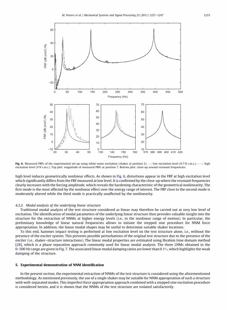
Fig. 6. Measured FRFs of the experimental set-up using white-noise excitation (shaker at position 2). —: low excitation level (0.7 N r.m.s.); - - -: high

excitation level (9 N r.m.s.). Top plot: magnitude of measured FRFs at position 7. Bottom plot: close-up around resonant frequencies.


high level induces geometrically nonlinear effects. As shown in Fig. 6, distortions appear in the FRF at high excitation levelwhich significantly differs from the FRF measured at low level. It is confirmed by the close-up where the resonant frequenciesclearly increases with the forcing amplitude, which reveals the hardening characteristic of the geometrical nonlinearity. Thefirst mode is the most affected by the nonlinear effect over the energy range of interest. The FRF close to the second mode ismoderately altered while the third mode is practically unaffected by the nonlinearity.

4.2.2. Modal analysis of the underlying linear structure

Traditional modal analysis of the test structure considered as linear may therefore be carried out at very low level ofexcitation. The identification of modal parameters of the underlying linear structure then provides valuable insight into thestructure for the extraction of NNMs at higher energy levels (i.e., in the nonlinear range of motion). In particular, thepreliminary knowledge of linear natural frequencies allows to initiate the stepped sine procedure for NNM forceappropriation. In addition, the linear modal shapes may be useful to determine suitable shaker locations.

To this end, hammer impact testing is performed at low excitation level on the test structure alone, i.e., without thepresence of the exciter system. This prevents possible perturbations of the original test structure due to the presence of theexciter (i.e., shaker–structure interactions). The linear modal properties are estimated using Ibrahim time domain method[28], which is a phase separation approach commonly used for linear modal analysis. The three LNMs obtained in the0–500 Hz range are given in Fig. 7. The associated linear modal damping ratios are lower than 0:1%, which highlights the weakdamping of the structure.

5. Experimental demonstration of NNM identification

In the present section, the experimental extraction of NNMs of the test structure is considered using the aforementionedmethodology. As mentioned previously, the use of a single shaker may be suitable for NNM appropriation of such a structurewith well-separated modes. This imperfect force appropriation approach combined with a stepped sine excitation procedureis considered herein, and it is shown that the NNMs of the test structure are isolated satisfactorily.

1 2 3 4 5 6 70

0.2

0.4

0.6

0.8

1 2 3 4 5 6 7−0.8

−0.4

0

0.4

0.8

1 2 3 4 5 6 7−0.8

−0.4

0

0.4

0.830.25 Hz 143.03 Hz 394.64 Hz

Sensor positionSensor positionSensor position

Fig. 7. Linear normal modes of the test structure identified at low excitation level in the 0–500 Hz range. From left to right: first, second and third

normal modes.


5.1. Experimental extraction of the first NNM

5.1.1. NNM force appropriation using stepped sine excitation

To minimize shaker–structure interaction, the shaker is placed near the clamped end of the main beam. For the first mode, theexciter is located at position 2 (see Fig. 4). The generated force is a single-sine (i.e., mono-harmonic) excitation of tunable frequency.

Based on the knowledge of the underlying linear properties, the stepped sine excitation procedure may be initiated usingthe natural frequency of the LNM as excitation frequency. In view of the hardening nonlinear behavior observed previously, itis gradually increased to follow the forced response branch of interest until resonance. At each step, if the excitationfrequency increment leads to a sudden change in the measured responses (i.e., discontinuity in the amplitude and phase ofthe motion) indicating a jump to another coexisting stable solution, the procedure is then restarted, and the last increment isdecreased to remain on the initial branch of forced responses. This procedure is stopped when sufficiently good NNMappropriation is achieved. To this end, the indicator introduced previously is continuously monitored during the process.

It is worth noticing that the shaker amplification does not operate at constant current source, but the generated voltage israther fixed during the experiments. As a result, the amplitude and phase of the actual force introduced by the exciter mayfluctuate during the stepped sine procedure. It is of little importance since the applied force is measured during experimentaltesting, which enables to determine the phase lag between the responses and the excitation, this latter being relevant herein.

The measured steady-state forced responses are illustrated in Fig. 8. The maximum amplitude of the displacement at the mainbeam tip is depicted as a function of the excitation frequency. The fundamental complex Fourier coefficients (i.e., corresponding tothe forcing frequency) of the measured acceleration responses along the structure are also given in phase scatter diagrams.Initially, quite large increments of the excitation frequency are suitable. Close to resonance, smaller variations are required toremain on the frequency response branch of interest. Another branch of stable periodic motions coexists near the resonance, andthe basin of attraction of the initial forced responses gets smaller as the frequency increases. From a practical viewpoint, the NNMappropriation is then realizable by carefully changing the frequency of the generated excitation. For instance, increments of 0.1 Hzare finally necessary during the stepped sine procedure to prevent jump phenomenon.

The scatter plots display the evolution of the phase of the forced responses with respect to the sine excitation which isalong the vertical axis (purely imaginary excitation). The motion across the structure is synchronous, and the phase lagchanges with the excitation frequency to come close to 901. It is confirmed by the evolution of the NNM appropriationindicator depicted in Fig. 9 which tends to 1. The proposed indicator, calculated from the measured accelerations across thestructure, is initially evaluated for each of the significant harmonics included in the responses (i.e., for the fundamental, thirdand fifth harmonics). The global NNM purity indicator combining all these harmonics is also displayed in this figure. Only oddharmonics are considered herein, even harmonic components of the responses being negligible (see Fig. 10). In particular, theevolution observed for the fundamental frequency indicator is in agreement with the change noticed by the scatter diagrams.On the other hand, multiple quadratures of the harmonic components occur prior to the one of the fundamental frequencyterms. It is evidenced by the existence of several unit values of the indicator for the harmonics of the fundamental frequency,which explains that the evolution of the global NNM indicator is not a monotonically increasing function. Eventually, theforced response obtained for the final excitation frequency of 39.91 Hz corresponds to a value of the indicator very close to 1for all harmonics. The global NNM appropriation indicator is thus equal to 0.99. This very satisfactory value reveals that thestructure practically vibrates synchronously with a phase lag of 901 with respect to the harmonic excitation. For eachmeasured response along the beam, a phase lag of 891 is actually observed for each harmonic.

As a result, the first undamped NNM is experimentally isolated at a specific energy level with good approximation. Themeasured time series of this resulting forced response are represented in Fig. 10. The displacement amplitude of the responseat the main beam end is about 1.2 mm. The nonlinearity is then activated, and harmonic components of the excitationfrequency appear in the response as clearly noticed by the power spectral density (PSD) shown in Fig. 10. The NNM modalcurve, expressing the motion in a two-dimensional projection of the configuration space, is given in Fig. 11 in terms ofaccelerations. This figure also represents the NNM modal shape composed of the maximum amplitudes of the accelerationsfor all measurement locations along the structure. The modal shape is a snapshot of the NNM motion at a specific time instantcorresponding to the maximum amplitude of the response.

28 30 32 34 36 38 402

4

6

8

10

12

14x 10−4

Frequency(Hz)

ω = 29 Hz

2 4 6 8

30

210

60

240

90

270

120

300

150

330

180 0

ω = 33 Hz

10

2030

210

60

240

90

270

120

300

150

330

180 0

ω = 37 Hz

20

4030

210

60

240

90

270

120

300

150

330

180 0

ω = 39 Hz

20

40

60

30

210

60

240

90

270

120

300

150

330

180 0

ω = 39.7 Hz

20

40

60

30

210

60

240

90

270

120

300

150

330

180 0

ω = 39.91 Hz

20

40

60

30

210

60

240

90

270

120

300

150

330

180 0

Max

imum

am

plitu

de (m

)

Fig. 8. Force appropriation of the first NNM of the test structure through experimental stepped sine excitation procedure. Top plot: Measured steady-state

periodic forced responses (marked by circles) given in terms of the maximum amplitude of the displacement at the main beam tip (i.e., at position 7) as a

function of the excitation frequency. Bottom plots: phase scatter diagrams of the fundamental complex Fourier coefficients of the measured accelerations

(m/s2) across the beam (i.e., positions from 1 to 7) at different excitation frequencies.


5.1.2. NNM free decay identification

Now that the structure vibrates according to the first NNM at a specific energy level, the gain of the exciter amplifier is turnedoff to initiate NNM free decay. The resulting response is illustrated in Fig. 12 where the time series of the measured displacement atthe beam end is depicted. The dashed line corresponds to the time instant when the shaker is stopped, i.e., the boundary betweenthe steady-state forced response (NNM force appropriation step) and the free damped motion (NNM free decay step).

In practice, the applied excitation does not immediately drop to zero at the turn-off instant. Nevertheless, the excitationrapidly reduces and can be assumed as negligible. It confirms that the influence of the presence of the exciter device on the

28 30 32 34 36 38 400

0.2

0.4

0.6

0.8

1

28 30 32 34 36 38 400

0.2

0.4

0.6

0.8

1

28 30 32 34 36 38 400

0.2

0.4

0.6

0.8

1

28 30 32 34 36 38 400

0.2

0.4

0.6

0.8

1

Frequency (Hz) Frequency (Hz)

Frequency (Hz)Frequency (Hz)

1st-h

arm

onic

indi

cato

r ∆1

3rd-

harm

onic

indi

cato

r ∆3

5th-

harm

onic

indi

cato

r ∆5

Glo

bal i

ndic

ator

∆

Fig. 9. Evolution of the NNM force appropriation indicator for the first NNM of the test structure with respect to the excitation frequency. Indicator for (a) the

fundamental frequency, (b) the third harmonic, (c) the fifth harmonic components, and (d) global NNM appropriation indicator.


free decay of the initial test structure of interest may be viewed as moderate. Finally, in view of the weak damping of thestructure and thanks to the invariance principle, the induced free damped response is expected to follow the first undampedNNM when energy decreases with time.

The continuous wavelet transform (CWT) is computed to track the frequency content of the measured single-NNM freedecay response as energy decreases. For illustration, the time–frequency dependence given by the CWT of the displacementmeasured at the beam tip is represented in Fig. 13. The temporal evolution of the instantaneous fundamental frequency isdetermined from the maximum ridge of the transform. The frequency–energy dependence of the first NNM is then extractedfrom the measured time series. This dependence can be clearly highlighted by substituting the response amplitude for time.The identified frequency as a function of the amplitude (envelope) of the displacement at the end of the main beam isillustrated in Fig. 14. In Section 6.3, the total energy present in the system is estimated, and the experimental FEP is fullyreconstructed from these measured data.

The modal curves of the first NNM are directly extracted from the measured time series around specific time instants,related to different energy levels. The first NNM at five distinct response levels corresponding to the squares in Fig. 14 isdisplayed in Fig. 15. This plot presents the identified modal curves and the associated modal shapes.

Figs. 14 and 15 clearly reveal that the first NNM and its oscillation frequency are strongly affected by nonlinearity forincreasing energy levels. The frequency increases with the energy level which confirms the hardening characteristic of thestructure. The NNM motions have also a marked energy dependence. At high energy, the modal curves distinctly deviate froma straight line, which reveals the higher harmonic contents (mostly the third harmonic) in the response. It is particularlypronounced given that the motion is represented in terms of accelerations. The modal shape is also altered as shown in Fig. 15.At low energy, the NNM thus comes close to the first LNM identified previously. In particular, the modal curve tends to astraight line in the configuration space and the NNM frequency corresponds to the natural frequency of the first linear mode.

5.2. Experimental extraction of the second NNM

5.2.1. NNM force appropriation using stepped sine excitation

In view of its deformation shape, the second mode is more sensitive to the presence of the exciter device in proximity to itsantinode of vibration. It was evidenced by experimental investigations. The shaker is consequently positioned closer to theclamped end of the main beam (namely at location 1) for the extraction of the second NNM.

0 0.05 0.1 0.15−2

−1

0

1

2 x 10–3

Dis

pl. 7

(m)

Time (s)

0 0.05 0.1 0.15−100

−50

0

50

100

Acc

. 7 (m

/s2 )

Time (s)

0 0.05 0.1 0.15−100

−50

0

50

100

Acc

. 5 (m

/s2 )

Time (s)

0 0.05 0.1 0.15−60−40−20

0204060

Acc

. 3 (m

/s2 )

Time (s)

0 50 100 150 200 250−350

−300

−250

−200

−150

−100

PS

D d

ispl

. 7 (d

B)

Frequency (Hz)

0 50 100 150 200 250−200

−150

−100

−50

0

50P

SD

acc

. 7 (d

B)

Frequency (Hz)

0 50 100 150 200 250−250−200−150−100

−500

50

PS

D a

cc. 5

(dB

)

Frequency (Hz)

0 50 100 150 200 250−150

−100

−50

0

50

PS

D a

cc. 3

(dB

)

Frequency (Hz)

Fig. 10. Appropriated forced response of the first NNM of the test structure (o¼ 39:91 Hz). Left plots: measured time series. Right plots: power spectral

density. From top to bottom: accelerations at position 3, position 5, position 7 and displacement at the tip of the beam, i.e., at position 7.

−60 −40 −20 0 20 40 60−80−60−40−20

020406080

1 2 3 4 5 6 70

20

40

60

80

Acc. at position 3 (m/s2)

Acc

. at p

ositi

on 7

(m/s

2 )

Acc

eler

atio

n (m

/s2 )

Sensor position

Fig. 11. Appropriated forced response of the first NNM of the test structure (o¼ 39:91 Hz). Left plot: Modal curve in a two-dimensional projection of the

configuration space in terms of measured accelerations. Right plot: Modal shape composed of the amplitudes of the measured accelerations along the

main beam.


0 2 4 6 8 10 12 14−2

−1

0

1

2 x 10−3

Dis

pl. 7

(m)

Time (s)

NNM forceappropriation

NNM free decay

Fig. 12. Free decay identification of the first NNM of the test structure. Measured free response initiated from the appropriated forced response

(o¼ 39:91 Hz). Time series of the displacement at the tip of the beam, i.e., at position 7. The dashed line corresponds to the turn-off time instant of the shaker,

i.e., the boundary between NNM force appropriation and NNM free decay.

0 2 4 6 8 10 12 1425

30

35

40

45

Freq

uenc

y (H

z)

Time (s)

NNM forceappropriation

NNM free decay

Fig. 13. Wavelet transform of the measured free decay of the first NNM of the test structure initiated from the appropriated forced response (o¼ 39:91 Hz).

Temporal evolution of the instantaneous frequency of the displacement at the tip of the beam, i.e., at position 7. The solid line corresponds to the maximum

ridge of the transform.

0 0.2 0.4 0.6 0.8 1 1.2x 10−3

25

30

35

40

45

Freq

uenc

y (H

z)

Amplitude of the displacement (m)

Fig. 14. Frequency of the first NNM of the test structure, identified from the measured free decay using the CWT, as a function of the amplitude displacement

at the main beam tip (i.e., at position 7). The solid line corresponds to the maximum ridge of the transform.


Similarly, the NNM force appropriation of the second mode is carried out by means of stepped sine excitation. Startingfrom the natural frequency of the second linear mode, the excitation frequency is next gradually increased. In Fig. 16, themeasured steady-state periodic responses resulting from this forced vibration testing are represented by means of the

−60 −40 −20 0 20 40 60−80−60−40−20

020406080

1 2 3 4 5 6 70

20

40

60

80


Acc

. at p

ositi

on 7

(m/s

2 )

Acc

eler

atio

n (m

/s2 )

Sensor position

Fig. 15. First NNM of the test structure extracted from the measured free decay at five different energy levels marked by squares in Fig. 14. Left plot: modal

curves in a two-dimensional projection of the configuration space in terms of measured accelerations. Right plot: modal shapes composed of the amplitudes

of the measured accelerations along the main beam.


amplitude displacement at the tip of the main beam. The fundamental frequency components of the forced frequencyresponses are also given in scatter plots. The corresponding evolution of the NNM appropriation indicator is illustrated inFig. 17. Similar results as for the force appropriation of the first NNM are observed. Regarding the practical realization, thefrequency of the excitation must nevertheless be adapted more carefully, which indicates narrower domain of attraction ofthe forced responses close to the second resonance. The NNM force appropriation is then performed for an excitationfrequency of 144.02 Hz that corresponds to a global NNM indicator of 0.99. At each measurement location, the phase lag of theresponses with respect to the excitation is thus about 891 for all harmonics. Accordingly, the second NNM practically vibratesin isolation. The measured modal curve and modal shape are displayed in Fig. 18.

From the considered location of the shaker, the magnitude of the induced response of the test structure is limited by themaximum force that can be generated by the exciter. For this higher-frequency mode, the displacement amplitude at the tipof the main beam that is reached during NNM force appropriation is then around 0.6 mm. However, as shown below (seeSection 6.3), the corresponding energy level of isolation is of the same order of magnitude than for the force appropriation ofthe first NNM. So, for this energy level of interest, the second mode seems to be moderately affected by nonlinearity. Theoscillation frequency of the isolated NNM motion is slightly altered in comparison with the natural frequency of the secondlinear mode: the frequency increases by only 1 Hz due to the hardening effect of the geometrical nonlinearity. In addition, theNNM modal shape does not almost differ from the corresponding linear mode. The isolated modal curve is practically astraight line in the configuration space, which illustrates the insignificance of higher harmonic components in the motion.

5.2.2. NNM free decay identification

As for the first NNM, the generated appropriate excitation is stopped by turning off the gain of the amplifier. Hence, themeasurement of the single-NNM free damped response enables to identify the energy dependence of the second NNM. Fig. 19shows the oscillation frequency identified from the time series using the CWT as a function of the displacement at the mainbeam end. The modal curves and the corresponding modal shapes extracted for five different energy levels (marked bysquares in Fig. 19) are depicted in Fig. 20.

It clearly illustrates the weak energy-dependence observed for the second NNM. The frequency and the modal curves areslightly affected by nonlinearity over the energy range under consideration.

Finally, the experimental extraction of the third NNM was not investigated in view of its quasi-independence on the energypresent in the system. As previously evidenced by the FRF measurements at low and high levels, the third mode is almost unaffectedby the nonlinearity for the considered energy range: the modal shape and the frequency remain unchanged from the LNM.

The previous results are corroborated in the next section which deals with the validation of these experimental results bymeans of the finite element model of the structure.

6. Finite element modeling and experimental validation

As mentioned previously, the proposed methodology for nonlinear EMA lies on moderate damping assumption, in whichcase the NNMs identified from experimental responses can be related to the NNMs of the underlying conservative system. Inthis section, a conservative finite element model of the test structure is considered. The theoretical modal analysis of thestructure is carried out using the numerical algorithm developed for NNM computation. The computed theoretical NNMsmay therefore be compared with the NNMs experimentally extracted using the modal testing methodology. From a practicalviewpoint, this overall procedure combining the theoretical and experimental modal analyses may be used in the context ofmodel validation of nonlinear structures. In this study, it is performed to assess the ability of the proposed methodology toextract the NNMs from experimental measurements. To this end, a reliable finite element model of the structure isindependently identified.

141.5 142 142.5 143 143.5 144 144.50

1

2

3

4

5

6

7 x 10−4

Frequency (Hz)

ω = 142 Hz

20

4030

210

60

240

90

270

120

300

150

330

180 0

ω = 143 Hz

100

20030

210

60

240

90

270

120

300

150

330

180 0

ω = 143.5 Hz

100

200 300

30

210

60

240

90

270

120

300

150

330

180 0

ω = 143.7 Hz

100

200

30030

210

60

240

90

270

120

300

150

330

180 0

ω = 143.9 Hz

200

400

30

210

60

240

90

270

120

300

150

330

180 0

ω = 144.02 Hz

200

400

30

210

60

240

90

270

120

300

150

330

180 0

Max

imum

am

plitu

de (m

)

Fig. 16. Force appropriation of the second NNM of the test structure through experimental stepped sine excitation procedure. Top plot: Measured steady-

state periodic forced responses (marked by circles) given in terms of the maximum amplitude of the displacement at the main beam tip (i.e., at position 7) as a

function of the excitation frequency. Bottom plots: phase scatter diagrams of the fundamental complex Fourier coefficients of the measured accelerations

(m/s2) across the beam (i.e., positions from 1 to 7) at different excitation frequencies.


6.1. Theoretical model of the test structure

The theoretical undamped model of the nonlinear test structure is obtained based on a finite element approach. Thegoverning equations of motion are then

M €xðtÞþKxðtÞþfnlfxðtÞg ¼ 0 ð8Þ

The underlying linear system (i.e., the mass and stiffness matrices M and K) is identified through the linear modal analysisperformed at low energy level. The nonlinear behavior (i.e., the nonlinear restoring force fnl) is next introduced in the model

142 142.5 143 143.5 1440

0.2

0.4

0.6

0.8

1

142 142.5 143 143.5 1440

0.2

0.4

0.6

0.8

1

Frequency (Hz) Frequency (Hz)

kth-

harm

onic

indi

cato

r ∆k

Glo

bal i

ndic

ator

∆

Fig. 17. Evolution of the NNM force appropriation indicator for the second NNM of the test structure with respect to the excitation frequency. Left plot:

indicator for the fundamental frequency (- - -) and third harmonic components (� � �). Right plot: global NNM appropriation indicator.

−400 −200 0 200 400400−500

−250

0

250

500

1 2 3 4 5 6 7−500

−250

0

250

500


Acc

. at p

ositi

on 7

(m/s

2 )

Acc

eler

atio

n (m

/s2 )

Sensor position

Fig. 18. Appropriated forced response of the second NNM of the test structure (o¼ 144:02 Hz). Left plot: Modal curve in a two-dimensional projection of the

configuration space in terms of measured accelerations. Right plot: Modal shape composed of the amplitudes of the measured accelerations along the

main beam.

0 1 2 3 4 5 6x 10−4

135

140

145

150

Freq

uenc

y (H

z)


Fig. 19. Frequency of the second NNM of the test structure, identified from the measured free decay using the CWT, as a function of the amplitude

displacement at the main beam tip (i.e., at position 7). The solid line corresponds to the maximum ridge of the transform.


by resorting to a nonlinear system identification method. It is worth pointing out that the finite element model consideredhere corresponds to the system studied in [17] regarding the numerical demonstration of the proposed methodology inwhich the parameters are now updated from experimental data.

6.1.1. Finite element model of the underlying linear structure

The finite element model of the test structure is illustrated in Fig. 21. The main beam and thin beam are modeled using14 and 3 two-dimensional Euler–Bernoulli beam elements, respectively. An additional linear rotational stiffness is used tomodel the junction between the two beams. Based on the linear modal parameters extracted in Section 4.2.2 by means oflinear modal testing at very low level, the updating of the model provides an estimation of the rotational stiffness term at thejunction.

−400 −200 0 200 400−500

−250

0

250

500

1 2 3 4 5 6 7−500

−250

0

250

500


Acc

. at p

ositi

on 7

(m/s

2 )

Acc

eler

atio

n (m

/s2 )

Sensor position

Fig. 20. Second NNM of the test structure extracted from the measured free decay at five different energy levels marked by squares in Fig. 19. Left plot: modal

curves in a two-dimensional projection of the configuration space in terms of measured accelerations. Right plot: modal shapes composed of the amplitudes

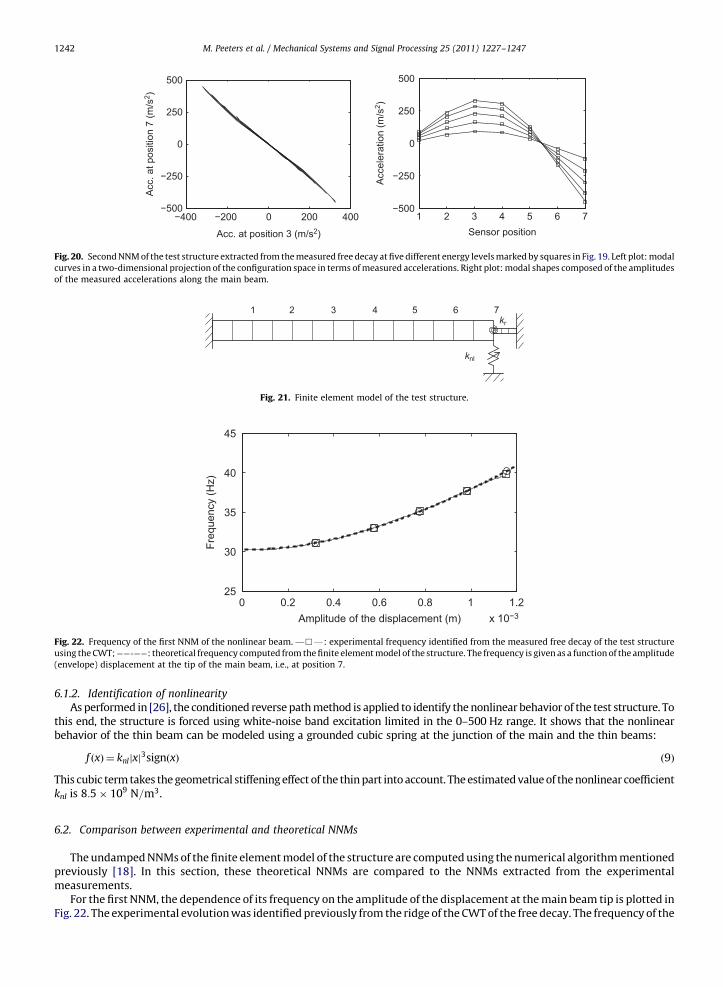
of the measured accelerations along the main beam.

knl

kr

1 2 3 4 5 6 7

Fig. 21. Finite element model of the test structure.

0 0.2 0.4 0.6 0.8 1 1.2x 10−3

25

30

35

40

45

Freq

uenc

y (H

z)


Fig. 22. Frequency of the first NNM of the nonlinear beam. —&F: experimental frequency identified from the measured free decay of the test structure

using the CWT;��3��: theoretical frequency computed from the finite element model of the structure. The frequency is given as a function of the amplitude

(envelope) displacement at the tip of the main beam, i.e., at position 7.


6.1.2. Identification of nonlinearity

As performed in [26], the conditioned reverse path method is applied to identify the nonlinear behavior of the test structure. Tothis end, the structure is forced using white-noise band excitation limited in the 0–500 Hz range. It shows that the nonlinearbehavior of the thin beam can be modeled using a grounded cubic spring at the junction of the main and the thin beams:

f ðxÞ ¼ knljxj3signðxÞ ð9Þ

This cubic term takes the geometrical stiffening effect of the thin part into account. The estimated value of the nonlinear coefficientknl is 8:5� 109 N=m3.

6.2. Comparison between experimental and theoretical NNMs

The undamped NNMs of the finite element model of the structure are computed using the numerical algorithm mentionedpreviously [18]. In this section, these theoretical NNMs are compared to the NNMs extracted from the experimentalmeasurements.

For the first NNM, the dependence of its frequency on the amplitude of the displacement at the main beam tip is plotted inFig. 22. The experimental evolution was identified previously from the ridge of the CWT of the free decay. The frequency of the


theoretical NNM closely matches the experimental one with a relative error lower than 1.25%. This error reaches itsmaximum value shortly after stopping the exciter. It could result from the imperfect realization of the free decay phasebecause of the presence of the exciter. Due to the existing coupling between the shaker and the structure, the appliedexcitation is not initially negligible which may lead to a parasitic deviation from the actual single-NNM free decay. In otherwords, the test structure of interest might be altered by interacting with the shaker system during the free decay step.However, this observed difference remains fully satisfactory and is rapidly reduced as evidenced in Fig. 22.

The experimental modal curves and modal shapes of this first NNM extracted from the NNM free decay at five differentenergy levels (marked by squares in Fig. 22) are depicted in Fig. 23. The left plots represent the modal curves in a two-dimensional projection of the configuration space while the right plots depict the modal shapes of the main beam. Forcomparison, the corresponding modal features of the theoretical NNM at the same five amplitude levels (marked by circles in

1 2 3 4 5 6 70

5

10

1515

1 2 3 4 5 6 70

10

20

30

1 2 3 4 5 6 70

10

20

30

4040

1 2 3 4 5 6 70

20

40

60

1 2 3 4 5 6 70

20

40

60

80

−10 −5 0 5 10−15−10

−505

101515

−15 −10 −5 0 5 10 1515−30−20−10

0102030

−20 −10 0 10 20−40

−20

0

20

40

−40 −20 0 20 40−60−40−20

020406060

−60 −40 −20 0 20 40 60−80

−40

0

40

8080

Acc. 3 (m/s2)

Acc

. 7 (m

/s2 )

Acc. 3 (m/s2)

Acc

.7 (m

/s2 )

Acc. 3 (m/s2)

Acc

. 7(m

/s2 )

Acc. 3 (m/s2)

Acc

. 7 (m

/s2 )

Acc. 3 (m/s2)

Acc

. 7 (m

/s2 )

Acc

. (m

/s2 )

Position

Acc

. (m

/s2 )

Position

Acc

. (m

/s2 )

Position

Acc

. (m

/s2 )

Position

Acc

. (m

/s2 )

Position

Fig. 23. First NNM of the nonlinear beam. —&F: experimental NNM identified from the free decay of the test structure; ��3��: theoretical NNM

computed from the finite element model of the structure. Left plots: modal curves in the configuration space composed of the accelerations at locations 3 and

7. Right plots: modal shapes composed of the amplitudes of the accelerations across the main beam. From top to bottom: NNM for decreasing energy levels

marked in Fig. 22.


Fig. 22) are also superimposed. From this figure, it is observed that the first NNM of the finite element model is in goodagreement with the experimental one for the complete energy range of interest.

Fig. 24 shows the comparison between the experimental and theoretical frequencies of the second NNM. For this weaklyenergy-dependent NNM, the observed deviation is insignificant. Indeed, the maximum relative error is about 0.3% andcorresponds to the initial difference in frequency resulting from the linear model updating, i.e., the error between the secondnormal mode of the updated underlying linear system and the experimental one extracted at low energy. The error on thefrequency of the second NNM is therefore satisfactory.

The modal curves and the modal shapes of this second NNM for three amplitude levels (marked in Fig. 24) are compared inFig. 25. It shows that the experimental and theoretical NNMs match very well throughout the different energy levels.

0 1 2 3 4 5 6x 10−4

140

142

144

146

148

150

Freq

uenc

y (H

z)


Fig. 24. Frequency of the second NNM of the nonlinear beam. —&F: experimental frequency identified from the measured free decay of the test structure

using the CWT;��3��: theoretical frequency computed from the finite element model of the structure. The frequency is given as a function of the amplitude

(envelope) displacement at the tip of the main beam, i.e., at position 7.

1 2 3 4 5 6 7−150−100

−500

50100150

1 2 3 4 5 6 7−400

−200

0

200

400

1 2 3 4 5 6 7

−400

−200

0

200

400

−100 −50 0 50 100−150−100

−500

50100150150

−300 −200−100 0 100 200 300−400

−200

0

200

400

−400 −200 0 200 400

−400

−200

0

200

400

Acc.3 (m/s2)

Acc

. 7 (m

/s2 )

Acc.3 (m/s2)

Acc

. 7 (m

/s2 )

Acc. 3 (m/s2)

Acc

. 7 (m

/s2 )

Acc

. (m

/s2 )

Position

Acc

. (m

/s2 )

Position

Acc

. (m

/s2 )

Position

Fig. 25. Second NNM of the nonlinear beam. —&F: experimental NNM identified from the free decay of the test structure; ��3��: theoretical NNM

computed from the finite element model of the structure. Left plots: modal curves in the configuration space composed of the accelerations at locations 3 and

7. Right plots: modal shapes composed of the amplitudes of the accelerations across the main beam. From top to bottom: NNM for decreasing energy levels

marked in Fig. 24.


In conclusion, these results confirm that the proposed methodology is capable of reliably extracting the energydependence of NNMs of the test structure from experimental measurements. Both a strongly and a weakly energy-dependentNNM have been identified.

6.3. Reconstructed frequency–energy plot (FEP)

From a physical viewpoint, it could be convenient to reconstruct the FEP of NNMs of the test structure from the obtainedexperimental results. This representation facilitates the interpretation of the dynamics. In particular, although the responseamplitude of the structure (e.g., the displacement at the tip of the main beam) provides a natural insight into the qualitativechange of energy in the system for a specific NNM, it cannot be used to compare the energy levels related to distinct NNMs.To this end, it is therefore necessary to determine the total energy (i.e., the sum of the kinetic and potential energies) presentin the structure from the experimental measurements.

Considering the general system (8), the expressions for the kinetic and potential energies are provided by

T ¼ 12_x�M _x ð10Þ

and

V ¼ 12x�KxþVnlðxÞ ð11Þ

respectively, where star denotes the transpose operation. In addition to the linear contribution, the potential energy iscomposed of the nonlinear termVnlðxÞ, which represents the strain energy associated to the nonlinear stiffness nonlinearities.The energy in the system, which is time dependent, may thus be estimated from the time response of the structure throughthe finite element model. Nevertheless, the response is only available at the measurement locations considered during theexperiments.

Following the philosophy of model reduction techniques [29], the total energy can then be expressed in terms of themeasured responses only. The equations of motions (8) of the conservative structural model can be partitioned as

MRR MRC

MCR MCC

" #€xR

€xC

" #þ

KRR KRC

KCR KCC

" #xR

xC

" #þ

fR,nlðxRÞ

0

� �¼

0

0

� �ð12Þ

where xR and xC are the vectors of the remaining and condensed DOFs, respectively. Keeping the nonlinear DOFs in theremaining coordinates, the equations of motion associated to the condensed DOFs are linear as evidenced by equation (12) inwhich the condensed part of the nonlinear restoring force fC,nl is zero. The finite element model can then be reduced usinglinear static condensation, commonly known as Guyan reduction method. This static condensation technique consists inneglecting the dynamic part of the condensed coordinates xC and thence expressing the global DOFs in terms of the remainingones as follows:

x¼xR

xC

" #¼ RxR ð13Þ

where R is the static reduction matrix given by

R¼I

�K�1CC KCR

" #ð14Þ

The reduced kinetic and potential energies are thus expressed as

T ¼ 12_x�RM _xR ð15Þ

V ¼ 12x�RKxRþVnlðxRÞ ð16Þ

with the nR � nR reduced structural matrices

M ¼R�MR

K ¼ R�KR ð17Þ

The expression for the nonlinear deformation energy Vnl is unchanged since it initially depends only on the nonlinear DOFswhich belongs to the remaining coordinates.

In order to estimate the energy from the available measurements, the remaining DOFs chosen here are the nodalcoordinates corresponding to the measurement locations across the structure. Hence, an estimation of the total energy can bedetermined using the expressions (15) and (16). Obviously, the quality of this estimation therefore depends on the numberand the positions of measured responses.

Targeting a general approach, the total energy is estimated by evaluating the kinetic energy at the time instants when thedisplacements pass through zero, i.e., when the potential energy vanishes. Since the kinetic energy depends only on theparameters of the underlying linear system, that prevents resorting to the nonlinear parameters which are generally

10−4 10−3 10−2 10−125

30

35

40

45

10−4 10−3 10−2 10−1

Energy (J)

140

142

144

146

148

150

Freq

uenc

y (H

z)

Fig. 26. Frequency–energy plot of the NNMs of the nonlinear beam. Left plot: experimental FEP reconstructed from the NNM identification results using the

modal testing methodology. Right plot: theoretical FEP computed from the finite element model of the structure. The modal shapes composed of the

amplitudes of the accelerations (m/s2) across the main beam are inset.


unknown a priori in practice. On the other hand, the underlying linear model can be identified, prior to nonlinear modaltesting under consideration in this study, by means of traditional linear modal analysis performed at low energy level (i.e.,when the nonlinearities are of sufficiently low amplitude). Furthermore, the mass properties are generally better assessedand subject to less uncertainty than the stiffness properties. A good approximation of the model mass matrix could even bebuilt based only on the geometrical and mechanical properties of the experimental set-up. The resulting estimation of theenergy, determined from all the experimental measurements and the reduced mass matrix, is referred to as the reconstructedenergy of the system. Its degree of confidence therefore depends on the quality of the reduced mass matrix that is considered.

For the considered test structure, the established finite element model is condensed by keeping the translational DOFs atthe positions of the seven accelerometers which span the main beam. Based on this structural model, the displacement of themain beam end is the only nonlinear DOF and is then kept in the reduction. Since the evaluation of the kinetic energy requiresthe velocities, the time responses measured in terms of acceleration are then numerically integrated.

The instantaneous energy in the system during the NNM free decay of the nonlinear modal testing is then evaluated fromthe experimental measurements. The experimental FEP is reconstructed through the CWT by substituting the estimatedinstantaneous energy for time. The maximum ridge of the transform therefore provides the experimental backbone of theNNM expressing its frequency–energy dependence. The reconstructed experimental FEP of the first and second NNMs isdepicted in Fig. 26. The experimental modal shapes extracted previously for different energy levels are also superimposed inthe plot. For comparison, the theoretical FEP numerically computed from the finite element model is also displayed in thisfigure. It again shows the good agreement between the theoretical and experimental NNMs.

Finally, the quality of the energy estimation can be assessed from the finite element model. It is observed that the reducedenergy is very close to the actual energy present in the system. For the first two NNMs, the theoretical FEPs given in terms ofthe actual energy or the reduced energy cannot be distinguished. It confirms that the reconstructed energy gives an excellentquantitative insight into the total energy in the structure.

7. Conclusion and future work

This paper deals with the experimental demonstration of the nonlinear phase resonance methodology proposed for EMAof nonlinear vibrating structures. To this end, a set-up composed of a nonlinear beam with geometrical nonlinearity wasconsidered. Based on a nonlinear extension of the phase quadrature criterion, an indicator was introduced for assessing thequality of NNM force appropriation. The experimental realization of NNM force appropriation was completed by means of astepped sine procedure using a single exciter at a single frequency. Finally, the energy dependence of NNM was properlyidentified from the measured single-NNM free decay response, which indicates the robustness of the procedure.


This two-step methodology, which can be applied to strongly nonlinear structures, therefore promises to progress towardpractical nonlinear EMA. In particular, this approach may be directly and fully integrated into the strategy currently followedfor standard ground vibration testing of aircrafts. In fact, besides traditional linear modal analysis performed using phaseseparation methods, it is common to resort to classical force appropriation for some particular modes. In case of modesaffected by nonlinearity, the proposed nonlinear phase resonance may therefore be realized, which extends the strategy tononlinear structures. Through the combination of EMA with theoretical modal analysis, finite element model updating andvalidation of nonlinear structures are also within reach.

More complex structures (e.g., structures possessing close modes or spatially distributed nonlinearities) will be addressedin future research. To this end, the development of a more general constructive procedure for NNM force appropriation,resorting to several shakers with harmonics of the fundamental frequency, could be necessary to ensure the robustness of themethodology. An assumption considered throughout this paper is that the damped dynamics can be interpreted based on theNNMs of the underlying conservative system. This issue deserves more attention and will be investigated in further studies.

References

[1] M. Degener, Ground vibration testing for validation of large aircraft structural dynamics, in: Proceedings of the International Forum on Aeroelasticityand Structural Dynamics, Manchester, UK, 1995.

[2] M. Degener, J. Gschwilm, S.P. Lopriore, R.S. Capitanio, V.E. Hill, P.W. Johnston, Vibration tests for dynamic verification and qualification of the ppf/envisat-1 satellite, in: Proceedings of the 3rd International Symposium on Environmental Testing for Space Programmes—ESA SP-408, Noordwijk, TheNetherlands, 1997, pp. 83–90.

[3] M. Degener, Experiences in large satellite modal survey testing, in: Proceedings of the European Conference on Spacecraft Structures, Materials andMechanical Testing—ESA SP-428, Braunschweig, Germany, 1998, pp. 659–664.

[4] J.R. Wright, J.E. Cooper, M.J. Desforges, Normal-mode force appropriation—theory and application, Mechanical Systems and Signal Processing 13 (2)(1999) 217–240.

[5] G. Kerschen, K. Worden, A.F. Vakakis, J.C. Golinval, Past present and future of nonlinear system identification in structural dynamics, MechanicalSystems and Signal Processing 20 (3) (2006) 505–592.

[6] S. Tsakirtzis, Y.S. Lee, A.F. Vakakis, L.A. Bergman, D.M. McFarland, Modeling of nonlinear modal interactions in the transient dynamics of an elastic rodwith an essentially nonlinear attachment, Communications in Nonlinear Science and Numerical Simulation 15 (2010) 2617–2633.

[7] Y.S. Lee, S. Tsakirtzis, A.F. Vakakis, D.M. McFarland, L.A. Bergman, Physics-based foundation for empirical mode decomposition: correspondencebetween intrinsic mode functions and slow flows, AIAA Journal 47 (2009) 2938–2963.

[8] Y.S. Lee, A.F. Vakakis, D.M. McFarland, L.A. Bergman, Non-linear system identification of the dynamics of aeroelastic instability suppression based ontargeted energy transfers, The Aeronautical Journal of the Royal Aeronautical Society 114 (2010) 61–82.

[9] W. Szemplinska-Stupnicka, The modified single mode method in the investigations of the resonant vibrations of non-linear systems, Journal of Soundand Vibration 63 (4) (1979) 475–489.

[10] W. Szemplinska-Stupnicka, Non-linear normal modes and the generalized Ritz method in the problems of vibrations of non-linear elastic continuoussystems, International Journal of Non-Linear Mechanics 18 (2) (1983) 149–165.

[11] S. Setio, H.D. Setio, L. Jezequel, A method of non-linear modal identification from frequency response tests, Journal of Sound and Vibration 158 (3)(1992) 497–515.

[12] S. Setio, H.D. Setio, L. Jezequel, Modal analysis of nonlinear multi-degree-of-freedom structures, The International Journal of Analytical andExperimental Modal Analysis 7 (2) (1992) 75–93.

[13] Y.H. Chong, M. Imregun, Development and application of a nonlinear modal analysis technique for mdof systems, Journal of Vibration and Control 7(2001) 167–179.

[14] C. Gibert, Fitting measured frequency response using non-linear modes, Mechanical Systems and Signal Processing 17 (1) (2003) 211–218.[15] M.F. Platten, J.R. Wright, G. Dimitriadis, J.E. Cooper, Identification of multi-degree of freedom non-linear systems using an extended modal space model,

Mechanical Systems and Signal Processing 23 (1) (2009) 8–29.[16] P.A. Atkins, J.R. Wright, K. Worden, An extension of force appropriation to the identification of non-linear multi-degree of freedom systems, Journal of

Sound and Vibration 237 (1) (2000) 23–43.[17] M. Peeters, G. Kerschen, J.C. Golinval, Dynamic testing of nonlinear vibrating structures using nonlinear normal modes, Journal of Sound and Vibration

330 (3) (2010) 486–509.[18] M. Peeters, R. Viguie, G. Serandour, G. Kerschen, J.C. Golinval, Nonlinear normal modes, Mechanical Systems and Signal Processing 23 (1) (2009)

195–216.[19] A.F. Vakakis, L.I. Manevitch, Y.V. Mikhlin, V.N. Pilipchuk, A.A. Zevin, Normal Modes and Localization in Nonlinear Systems, Wiley Series in Nonlinear

Science, John Wiley & Sons, New York, 1996.[20] G. Kerschen, M. Peeters, J.C. Golinval, A.F. Vakakis, Nonlinear normal modes, Mechanical Systems and Signal Processing 23 (1) (2009) 170–194.[21] R.M. Rosenberg, Normal modes of nonlinear dual-mode systems, Journal of Applied Mechanics 27 (1960) 263–268.[22] R.M. Rosenberg, The normal modes of nonlinear n-degree-of-freedom systems, Journal of Applied Mechanics 30 (1) (1962) 7–14.[23] R.M. Rosenberg, On nonlinear vibrations of systems with many degrees of freedom, Advances in Applied Mechanics 242 (9) (1966) 155–242.[24] C. Touze, M. Amabili, Nonlinear normal modes for damped geometrically nonlinear systems: application to reduced-order modelling of harmonically

forced structures, Journal of Sound and Vibration 298 (4–5) (2006) 958–981.[25] F. Thouverez, Presentation of the ECL benchmark, Mechanical Systems and Signal Processing 17 (1) (2003) 195–202.[26] G. Kerschen, V. Lenaerts, J.C. Golinval, Identification of a continuous structure with a geometrical non-linearity, Journal of Sound and Vibration 262 (4)

(2003) 889–906.[27] V. Lenaerts, G. Kerschen, J.C. Golinval, Identification of a continuous structure with a geometrical non-linearity part II: proper orthogonal

decomposition, Journal of Sound and Vibration 262 (4) (2003) 907–919.[28] S.R. Ibrahim, E.C. Mikulcik, A time domain modal vibration test technique, The Shock and Vibration Bulletin 43 (1973) 21–37.[29] M. Geradin, D. Rixen, Mechanical Vibrations: Theory and Application to Structural Dynamics, Wiley, Chichester, 1994.

Documents

Mechanical Systems and Signal Processing - uliege.be · Mechanical Systems and Signal Processing 25 ... sine wave at the undamped natural frequency of a linear mode and enables small