Embed Size (px)
Citation preview

Mechanisms of loss of high energy protons from the bunched
beams in storage rings
Dissertation
zurErlangung des akademischen Grades
Doktor-Ingenieur (Dr.-Ing.)
der Fakultat fur Ingenieurwissenschaftender Universitat Rostock
vorgelegt von
Ilya Agapovaus Moskau
Rostock2004

Gutachter der Dissertation: Prof. Dr. Ursula van Rienen, Universitat RostockDr. Ferdinand Willeke, DESY Hamburg

Preface
This work is dedicated to the analysis of some aspects of long term beam behavior in a storage ring whenrandom perturbations are present. The techniques discussed are fairly general and can be applied to awide range of problems, but here we will concentrate on the study of synchrotron motion of bunchedbeams of heavy particles like protons or ions. This study is motivated by the coasting beam productionobserved in the HERA proton accelerator, which was found to contribute to background in the detectors.We study the evolution of the longitudinal bunch distribution under the influence of two kinds of randomperturbations: jump processes and continuous fluctuations. The first type models scattering processes likethe Touschek effect and gas scattering, the second models processes such as RF field noise. The questionwe want to answer is which role do these phenomena play in the longitudinal tail buildup and coastingbeam production. The physics of these processes is well understood at present, but, to our knowledge, theeffect of nonlinearity on the tail evolution and on the escape rate has not been fully studied. Appropriatemethods are discussed and simulations are compared to experimental observations at HERA.
i

ii

Contents
1 Introduction 1
2 Probability background 5
2.1 Random variables and Markov chains . . . . . . . . . . . . . . . . . . . . . . . . . . . . . 5
2.2 Continuous random processes . . . . . . . . . . . . . . . . . . . . . . . . . . . . . . . . . . 6
3 Discrete random perturbations and the Touschek effect 13
3.1 The Touschek effect and the intra-beam scattering . . . . . . . . . . . . . . . . . . . . . . 13
3.2 Kinetic equations . . . . . . . . . . . . . . . . . . . . . . . . . . . . . . . . . . . . . . . . . 17
3.3 Averaging of the kinetic equations . . . . . . . . . . . . . . . . . . . . . . . . . . . . . . . 18
3.4 The diffusion (Fokker-Planck) approximation . . . . . . . . . . . . . . . . . . . . . . . . . 20
3.5 Reduction to a linear integro-differential equation . . . . . . . . . . . . . . . . . . . . . . . 22
3.6 Solution of the Boltzmann equation (method of self-consistent chains). . . . . . . . . . . . 22
3.6.1 Self-consistent chains . . . . . . . . . . . . . . . . . . . . . . . . . . . . . . . . . . . 22
3.6.2 Computation procedure . . . . . . . . . . . . . . . . . . . . . . . . . . . . . . . . . 25
3.6.3 Results for HERA . . . . . . . . . . . . . . . . . . . . . . . . . . . . . . . . . . . . 26
3.7 Summary . . . . . . . . . . . . . . . . . . . . . . . . . . . . . . . . . . . . . . . . . . . . . 27
4 RF noise 33
4.1 Randomly perturbed synchrotron oscillations . . . . . . . . . . . . . . . . . . . . . . . . . 33
4.2 The averaged Fokker-Planck equation . . . . . . . . . . . . . . . . . . . . . . . . . . . . . 38
4.3 Effect of coherence . . . . . . . . . . . . . . . . . . . . . . . . . . . . . . . . . . . . . . . . 49
4.4 Solving the Fokker-Planck equation . . . . . . . . . . . . . . . . . . . . . . . . . . . . . . . 51
4.4.1 A two-point boundary value problem . . . . . . . . . . . . . . . . . . . . . . . . . . 52
4.4.2 The system of equations with coupled boundary values arising from averaging ofstochastic systems with complicated phase space where branching can occur . . . . 54
4.4.3 On the mechanism of separatrix crossing . . . . . . . . . . . . . . . . . . . . . . . . 55
4.4.4 On numerical solution of the coupled system . . . . . . . . . . . . . . . . . . . . . 56
4.5 Impact on synchrotron motion . . . . . . . . . . . . . . . . . . . . . . . . . . . . . . . . . 59
4.5.1 Bunch diffusion - rough estimates . . . . . . . . . . . . . . . . . . . . . . . . . . . . 59
4.5.2 Escape from the stable bucket . . . . . . . . . . . . . . . . . . . . . . . . . . . . . 60
4.5.3 On effects of noise spectral density . . . . . . . . . . . . . . . . . . . . . . . . . . . 60
4.5.4 Estimates for HERA . . . . . . . . . . . . . . . . . . . . . . . . . . . . . . . . . . . 60
4.6 Summary . . . . . . . . . . . . . . . . . . . . . . . . . . . . . . . . . . . . . . . . . . . . . 62
iii

iv CONTENTS
5 Some experimental observations 715.1 Backgrounds and longitudinal bunch evolution . . . . . . . . . . . . . . . . . . . . . . . . 715.2 Bunch manipulations with amplitude and phase modulations . . . . . . . . . . . . . . . . 735.3 Summary . . . . . . . . . . . . . . . . . . . . . . . . . . . . . . . . . . . . . . . . . . . . . 75
6 Epilogue 776.1 Noise in nonlinear systems . . . . . . . . . . . . . . . . . . . . . . . . . . . . . . . . . . . . 776.2 Conclusion . . . . . . . . . . . . . . . . . . . . . . . . . . . . . . . . . . . . . . . . . . . . 78
A Particle motion in a storage ring 79A.1 Equations of motion . . . . . . . . . . . . . . . . . . . . . . . . . . . . . . . . . . . . . . . 79A.2 Action-angle variables . . . . . . . . . . . . . . . . . . . . . . . . . . . . . . . . . . . . . . 82
B Sketch of the proof of proposition 1 87
C On the precision of the ’self-consistent chains’ method 91

Some frequently used symbols
e electron chargeεx,y vertical and horizontal emittancesβx,y verticcal and horizontal beta functionsβ, γ relativistic factorsσx,y,s r.m.s. beam sizesωRF frequency of an RF cavity resonatork(τ) the autocorrelation functionξt a equivalent to ξ(t)Sξ(ω) spectral power density of a random process ξpi,j transition probabilities of a Markov processWt the Wiener processdWt white noiseH(q, p) the Hamiltonian
v


Chapter 1
Introduction
For modern collider physics experiments, like those installed at HERA, beams of high intensity are needed,so that the luminosity is high and there are sufficient physics event statistics. HERA is a lepton-protonstorage ring at DESY Hamburg (see figure 1.1) , with the following experiments operating
• The experiments designed to understand proton structure by colliding a proton beam with an electronbeam - H1 and ZEUS
• Nucleon spin study by colliding polarized electrons/positrons with a fixed target of polarized nucleons- HERMES
• Study of heavy C- and B- quark production and CP violation using a fixed wire target - the HERA-Bexperiment.
Table 1.1: Main parameters of the HERA ep collider
circumference 6355mproton energy 920 GeVlepton energy 27.5 GeVnumber of colliding bunches 174design p bunch intensity Np 1 · 1011
design e current Ie 60mAlongitudinal e spin polarization 50-70%design peak luminosity 7 · 1031cm−2s−1
proton envelope function at IP’s βz,x 18cm, 2.45mtypical proton emittances εz,x 5nmlepton beam size at the IP’s σz,x 30, 114µmproton bunch length 200mmlepton bunch length 8mm
For ep bunched beam collisions the luminosity (per collision, Gaussian beams) is
L = RIeNp
2πe√
(σ2x,p + σ2
x,e)(σ2z,p + σ2
z,e)(1.1)

2 Introduction
with R being a reduction factor, which depends on the β function at the interaction point, the p bunchlength 1 and the crossing angle [11]. With nonzero crossing angle and bunched beams high luminosityis achieved by creating bunches with small transverse and longitudinal dimensions and bringing themproperly into collision. Beams of high intensity can produce high background rates at the detectors, sothat the detector components suffer from radiation damage and data cannot be taken.
High background has been a substantial problem for experiments at HERA. Its potential sources are
• Direct synchrotron radiation
• Backscattered synchrotron radiation
• Bremsstrahlung and lepton background produced by leptons scattered at the residual gas
• Proton halo
• Protons scattered at the desorbed gas in the interaction regions
All these can, in principle, be controlled by beam steering, by putting masks and absorbers in thecritical regions and by providing a good vacuum pressure around the detectors.
In addition a connection between the background and the coasting beam observed at HERA-p hasbeen suggested. The coasting beam is formed by particles that leave the stable RF buckets and drift inthe longitudinal direction along the ring. The synchrotron radiation losses are no more compensated forsuch particles and they constantly lose energy. Due to dispersion they will have a large transverse offsetand form the beam halo. The chromatic tune shift due to large momentum offset also introduces a threatof hitting a resonance. The beam-beam force has a much stronger impact on off momentum particles (see[16],[59] for details). Due to all these effects the coasting beam particles are likely to escape the aperturelimitations rather quickly. Although the collimation system is designed to shield the detectors [54], someportion still ends up there and causes the background. In a superconducting accelerator it is difficult tocollimate off-momentum particles effectively. The collimator system has two stages: the first collimatordeflects a proton which then hits the secondary collimator. In the regions with high dispersion, the arcs,superconducting magnets are installed and putting a collimator next to one of such magnets may causea quench. Thus particles with momentum offset cannot be collimated efficiently. The collimation of thecoasting beam may also be performed by introducing transverse kicker magnets acting in the gap betweenthe bunches. The timing of the kicks must be very precise. Therefore, it is technically difficult to producea short clean rectangular kick since a signal with extremely large bandwidth would be required.
The observation of the coasting beam was first performed at the HERA-B experiment by analyzingthe scattering rates of the proton beam on the target wires [19]. Its existence has also been confirmedby measuring the difference between the bunched and unbunched currents and the results indicated thatthe accumulated coasting current (up to 2mA of approximately 100mA initial total current) must beconsiderably reduced to allow the experiments to operate. The coasting beam has also been observed atother machines such as RHIC [64].
High coasting beam current can have other consequences. For example, the particles filling the abortgap between the bunch trains can prevent a safe beam dump. This, for example, is expected to play arole at the LHC.
There could be several possible causes for the production of the coasting beam. These could possibly belongitudinal particle instabilities arising from the coupling of synchrotron and betatron motion, wake fields,noise in the radio frequency cavities, parasitic collisions and many others. Since the transverse protonbeam lifetime observed in HERA was satisfactory, we focused on the study of the escape mechanisms fromthe stable RF buckets due to the following phenomena: the Touschek effect (or intra-beam scattering) and
1this is the hourglass effect

3
Figure 1.1: Schematic overview of the HERA ep collider and its accelerator chain
noise in the radio-frequency system. Both processes may be considered to be small random perturbations.Deterministic perturbations to synchrotron motion are also taken into consideration to some extent.
The particles in a bunch experience collisions with each other, at high energies collisions may lead tolarge momentum jumps, which in turn lead to bunch size growth and to particle loss from the bunch.This process was recognized by B. Touschek in 1963 on a small e−e+ storage ring [7] and later studied bymany, including A. Piwinski [49], [50]. It is to be taken into account for high intensity beams like thosestored in HERA-p.
Noise is always present in the accelerating RF fields. Since the effect of radiation damping on the protonmotion in stable RF buckets is weak, even extremely small perturbations can accumulate and influencethe motion on large time scales. This influence was observed in all proton machines (such as SPS andHERA). The question arises: to what extent is the RF noise responsible for producing the coasting beam?
Deterministic perturbations also have a considerable influence on bunch motion. The major source ofsuch perturbations is assumed to come from the longitudinal impedances arising in beam-cavity interac-tions. As far as nonlinear single-particle motion is concerned, a deterministic perturbation will cause acomplicated effect, the so-called nonlinear resonance [12]. Under certain conditions it can lead to particleloss. The interplay of resonance with noise can also lead to interesting phenomena [25].
Synchrotron oscillations in HERA are of quite complicated nature due to the presence of two radiofrequency (RF) systems. The first, at 52 MHz, dominates at the injection energy of 40 GeV while thesecond, at 208 MHz, provides shorter bunches and dominates when the beam is stored at 920 GeV. Itis technically complicated to turn off the 52MHz system and the accelerating field seen by the beam isproduced by a two frequency system. For details see Appendix A. A simple analytical treatment of boththe Touschek effect and the RF noise problem is generally not possible for the bunch tail particles whichexhibit nonlinear behavior (which is the case for all RF systems as soon as the bunch size is of the orderof an RF wavelength). This motivated us to study the motion of nonlinear oscillating systems under theinfluence of various kinds of random perturbations more carefully, taking into account issues specific tosynchrotron motion in a storage ring and to develop appropriate simulation techniques.
The presentation has the following structure:In Chapter 2 basic facts from probability theory are briefly given for reference.In Chapter 3 modeling of the Touschek effect (or intra-beam scattering) is discussed [49], [9], [18]. Here
the nonlinearity of the RF potential introduces a difficulty. The statistical characteristics of a scatteringevent are expressed by some averaged functions over the particle trajectory taking into account the bunchdensity. For the tail particles it is too complicated to calculate calculating these averages analyticallyand computer simulations must be made. The tail distribution is important when the escape problemis concerned. The approaches to such simulations are discussed and calculations based on the “chainmethod” are presented.
4 Introduction
In Chapter 4 issues concerning simulation of the influence of RF noise on the synchrotron oscillationsare presented. So far only the sinusoidal RF voltage has been treated carefully [17], [32]. Obtaining andsolving a Fokker-Planck equation for the case of a double RF system is perhaps principally the same,but technically more elaborate. The following technical issues are discussed: averaging the Fokker-Planckequation, calculating the diffusion coefficient by perturbation techniques, solving the equation when thephase space includes separatrices and estimating the effect of noise coherence.
In Chapter 5 the corresponding observations in HERA-p are presented.Apparently, the major source of the coasting beam at HERA has been the influence of the RF noise
whereas the contribution of intra-beam scattering appears to be weak.In the last chapter we indicate other possible applications of the methods discussed as well as bottle-
necks arising in generalizing these techniques and some open questions.

Chapter 2
Probability background
This section shortly summarizes some well-known facts and definitions from the theory of probability andrandom processes following [21], [55] and can be skipped by those who are familiar with them. A goodintroduction to the theory of random processes and stochastic differential equations may be found in [21],[24], [55], more rigorous treatment is given in [22], [28], [29], [35].
2.1 Random variables and Markov chains
A random variable ξ(ω) is a measurable function defined on the space of elementary events Ω. Themoments of a random variable are
〈ξ〉 =
∫
Ω
ξ(ω)dω
⟨
ξ2⟩
=
∫
Ω
(ξ(ω) − 〈ξ〉)2 dω
. . . (2.1)
The characteristic function is
θ(u) =⟨
eiuξ⟩
(2.2)
The simplest special case of a random process is the Markov chain. A Markov chain is given by thespace of states (say, a subset of integers) and the transition probabilities from state i to state j in time tpij(t) satisfying
1. 0 ≤ pij(t) ≤ 1
2.∑
j pij(t) = 1
3. ∀t > 0, s > 0 pij(t+ s) =∑
k pik(t)pkj(s) (Chapman-Kolmogorov equation)
4. limt↓0 pij(t) = δij (stochastic continuity)
Then it can be shown that the following limits exist
aij = limt↓0
pij(t) − δijt
6 Probability background
If i 6= j then the limits are always bounded. Therefore, the transition probabilities satisfy the Kol-mogorov system of equations
d
dtpij(t) =
∑
k
aikpkj(t) (2.3)
The system possesses a unique solution if aij ≥ 0, aii ≤ 0,∑
aij = 0, sup |aii| < ∞ and the solutionsatisfies the initial conditions pik(0) = δik. These conditions are usually met in practice. The matrix aij isthe discrete analogy of an infinitesimal generator of a Markov process and will be called the infinitesimalgenerator matrix.
2.2 Continuous random processes
A random process ξ(t) is in general a random function taking values in an appropriate functional space.Assume that this is the space of all real-valued functions. A random process is defined if for every sett1, . . . tn the joint probability density of random variables ξ(ti) fn(x1, . . . xn, t1, . . . tn) is given, such that
∫
fn(x1, . . . , xn, t1, . . . tn)dx1 . . . dxn = 1 (2.4)
fn(x1, . . . , xn, t1 . . . tn) ≥ 0 (2.5)
fn(x1, . . . xi . . . xj . . . , xn, t1 . . . ti . . . tj . . . tn) =
fn(x1, . . . xj . . . xi . . . , xn, t1 . . . tj . . . ti . . . tn)
and
fn(x1, . . . xn, t1, . . . tn) =
∫
fn+k(x1, . . . xn+k, t1, . . . tn+k)dxn+1 . . . dxn+k
One also writes ξt instead of ξ(t) and f(xt1 . . . xtn) or f(x1 . . . xn) instead of fn(x1, . . . xn, t1, . . . tn) forbrevity. One defines the moment function of order n
mn(t1, . . . , tn) = 〈ξt1 . . . ξtn〉 (2.6)
with the usual notation ξt = ξ(t). The random process is defined by an infinite series of momentfunctions of all orders. The physical significance of a moment function decreases with the increase ofits order. In applications it is often sufficient to know only the first two functions m1(t) and m2(t1, t2).Equivalent to the knowledge of moment functions is the knowledge of the correlation functions
kn(t1 . . . tn) = K[ξ(t1) . . . ξ(tn)]
where K is the correlation between random variables. The second order correlation is
K[ξ1ξ2] = 〈ξ1ξ2〉 − 〈ξ1〉 〈ξ2〉 (2.7)
and the correlation of arbitrary order is given by
K[ξ1 . . . ξn] =1
in∂ ln Θ(u1 . . . un)
∂u1 . . . ∂un|u1=...un=0 (2.8)
where

2.2 Continuous random processes 7
Θ(u1 . . . un) = 〈expi(u1ξ1 + . . . unξn)〉 (2.9)
The process is called stationary (strict sense) if the moment functions (or correlation functions) areinvariant under time shifts
k1(t) = m1(t) = m
k2(t1, t2) = k2(0, t2 − t1) = k(t2 − t1)
. . .
and so on. For a stationary process one defines the correlation time and the process intensity
τcor =1
k(0)
∫ ∞
0
|k(τ)| dτ
K =
∫ ∞
−∞k(τ)dτ
The spectral density of a stationary process is
Sξ(ω) = 2
∫ ∞
−∞eiωτ 〈ξtξt+τ 〉 dτ = 4
∫ ∞
0
cos(ωτ) 〈ξtξt+τ 〉 dτ (2.10)
for a process with zero mean
Sξ(ω) = 2
∫ ∞
−∞eiωτk(τ)dτ (2.11)
for a process with mean 〈ξ〉 = m
Sξ(ω) = 2
∫ ∞
−∞eiωτk(τ)dτ + 4πm2δ(ω) (2.12)
for instance (see also figure 2.1)
k(τ) = e−γτ ⇒ S(ω) =4γ
ω2 + γ2
k(τ) = e−γτ cos(ω0τ) ⇒ S(ω) = 4γ4ω2 + ω2
0 + γ2
(ω2 − ω20 − γ2)2 + 4γ2ω2
(2.13)
For a multidimensional process (ξ1(t), ξ2(t)) one defines cross-correlation function
k12(t1, t2) = K[ξ1(t1), ξ2(t2)]
and cross-spectral density
Sξ1ξ2(ω) = 2
∫ ∞
−∞eiωτ < ξ1,tξ2,t+τ > dτ
The spectral density has to be distinguished from the random spectrum of the random process whichis a Fourier transform of a particular process sample
Y (ω) =1√2π
∫ ∞
−∞e−iωtξ(t)dt (2.14)

8 Probability background
Figure 2.1: Sample spectral densities
ω0
(a) Spectral density of a process withk(τ) = e−γ|τ |
ω
S
(b) Spectral density of a processwith k(τ) = e−γ|τ | cos(ω0τ)
This integral diverges for stationary random processes and has to be understood as a generalizedfunction. The spectral density has a meaning of the averaged noise spectrum. It has a meaning only ifwe consider the noise signal passed through a narrow band filter with ∆ω ∼ |ω − ω0| instead of a randomspectrum.
Y (ω0, t0) =
∫ ∞
−∞G(t0 − t)ξ(t)dt (2.15)
G(t0 − t) =1√2π
∫ ∞
−∞eiω(t0−t)g(ω)dω (2.16)
with g(ω) a pulse located in the interval ∆ω around ω0 and
∫ ∞
−∞g(ω)dω = 1 (2.17)
the connection between so filtered signal and the spectral density is
⟨
(Y (ω0, t0)2)⟩
=1
2Sξ(ω0)
∫ ∞
−∞|g(ω)|2 dω (2.18)
As has been mentioned, the first two moments already contain the most significant information aboutthe random process and the higher order moments are mostly responsible for extremal behavior. It is thennatural to consider a class of stationary processes with only the first two moments different from zero.Such processes are called second order processes. Their statistical properties are completely defined bythe correlation function K(τ).
A random process with K(τ) = Kδ(τ) is called a delta-correlated process or white noise with intensityK. It is an abstraction of a physical process with negligible correlation time. It has the advantage that itis a Markov process (see below), but it has infinite intensity and cannot be physically realized. A randomprocess with arbitrary K(τ) is also known as colored noise.
An important role is played by Markov random processes, or processes without after-effect. Let ξ(t) be arandom process and tn > tn1
> . . . > t1. The conditional probability density of ξ(tn) with ξ(tn−1) . . . ξ(t1)given is
f(xn|xn−1 . . . x1) =fn(xn . . . x1)
fn−1(x1 . . . xn−1)(2.19)

2.2 Continuous random processes 9
A process ξ(t) is called Markov if the conditional probability 2.19 depends on xn−1 only, i.e.
f(xn|xn−1 . . . x1) = ptn−1tn(xn−1, xn) (2.20)
pt1t2(ξ1ξ2) is called the transition probability of the Markov process. Markov processes possess aremarkable property, namely their transition probabilities satisfy the Chapman-Kolmogorov equation
pt1t3(x1, x3) =
∫
pt1t2(x1, x2)pt2t3(x2, x3)dx2 (2.21)
The Chapman-Kolmogorov equation is what makes Markov processes so significant. It provides amethod of calculating the evolution of probability density in time. For more general classes of randomprocesses such methods do not normally exist and they are usually treated by approximating them withan appropriate Markov process. The probability density f(x, t) describes the probability of finding therandom process at point x at time t and, in case of a Markov process, satisfies
f(x1, t1) =
∫
pt1t2(x1, x2)f(x2, t2)dx2 (2.22)
which is proved by integrating 2.21 over x3. Equation 2.21 can be reduced to a differential equation.
f(x) =
∞∑
n=1
(−1)n
n!
(
∂
∂x
)n
[Kn(x)f(x)] (2.23)
with
Kn(x) = limτ→0
〈(xτ − x)n〉τ
(2.24)
If the series 2.23 can be truncated at the second term then we get the Fokker-Planck or diffusionequation
f(x) = − ∂
∂x[K1(x)f(x)] +
1
2
∂2
∂x2[K2(x)f(x)] (2.25)
This possibility is equivalent to some regularity requirements on the paths of the random process (likecontinuity). The coefficients K1 and K2 are called the drift and diffusion coefficients. The Wiener process
or standard Brownian motion is a diffusion process with zero drift and unit diffusion. The trajectory ofa Wiener process is continuous but nowhere differentiable. One can however define the derivative of theWiener process dWt which happens to be the white noise process.
In applications physical processes are often given as solutions of differential equations. To be ableto treat equations with r.h.s. containing random processes one has to take advantage of the theory ofBrownian motion and stochastic differential equations. Suppose we are given a differential equation witha random r.h.s.
x = g(x, t, ω)
then it is natural to say that a solution is a function x(t) satisfying the integral equation
x(t) = x(0) +
∫ t
0
g(x(s), s, ω)ds (2.26)
But for many important random processes (like white noise) this integral does not exist in the usualRiemann-Steltjes sense. The theory of stochastic differential equations based on special integral definitionwas developed by Ito and Stratanovich. One starts with equations with white noise in the r.h.s

10 Probability background
dx
dt= a(x) + b(x)
dWt
dt
which is usually written in the form
dx = a(x)dt+ b(x)dWt
The solution is formally a random process satisfying the corresponding integral equation
x(t) = x(0) +
∫ t
0
a(x(s))ds +
∫ t
0
b(x(s))dWs (2.27)
The first integral is understood in the usual sense. The second one is an integral over a path of aWiener process and doesn’t exist in the usual sense [29]. It is defined in the following way. Let Π be apartition of interval [a, b] with points sii=1,n and ‖Π‖ = maxi=1,n−1 |si+1 − si|, then
∫ b
a
g(W )dWs = lim‖Π‖→0
∑
[
εg(Wsi) + (1 − ε)g(Wsi+1
)] [
Wsi+1−Wsi
]
(2.28)
Such an integral is called the stochastic integral. It exists for a large class of integrands and 2.27admits a solution. For different ε this defines different random processes. When ε = 0 the integral isin Ito’s sense, when ε = 0.5 Stratanovich’s. When a stochastic differential equation has a solution inStratanovich’s sense, then there exists a corresponding equation having the same solution in Ito’s sense.Ito’s integral could be defined for a somewhat broader class of integrands. Some important properties ofstochastic integrals are shown below
Ito Stratanovich
⟨∫ τ
0 dWs
⟩
= 0⟨∫ τ
0 dWs
⟩
= 0⟨
(∫ τ
0dWs
)2⟩
= τ⟨
(∫ τ
0dWs
)2⟩
= τ⟨∫ τ
0WsdWs
⟩
= 12W
2τ + τ
⟨∫ τ
0WsdWs
⟩
= 12W
2τ
f(Wt) = f(W0) +∫ t
0f ′(Ws)ds+ 1
2
∫ t
0f ′′(Ws)dWs f(Wt) = f(W0) +
∫ t
0f ′(Ws)ds
The last relation is known as the Ito’s rule. The multidimensional system
dx = a(x)dt+ b(x)dWt (2.29)
with a(x), b(x) ∈ Rn×n x ∈ Rn and W (t) ∈ Rn being n independent Wiener processes is treatedin complete analogy. Under a stochastic differential equation we will understand equations of type 2.29.Equations of general form are usually treated by reducing them to certain systems of (Ito or Stratanovich)stochastic equations [22] [28] [37].
One may pose various questions about solutions of the equations in question, such as first exit timefrom a domain etc. We are interested mainly in the evolution of the probability distribution supposingthe initial distribution is given. Solutions of stochastic differential equations are Markov processes andthus must satisfy a Chapman-Kolmogorov equation 2.21. One calculates its coefficients by substituting2.27 into 2.24 and exploiting the properties of stochastic integrals. For the Ito’s integral one gets
K1(x) = limτ→0
〈xτ − x〉τ
=
limτ→0
1
τ
⟨∫ τ
0
a(x(s))ds +
∫ τ
0
b(x(s))dWs
⟩
= a(x)

2.2 Continuous random processes 11
K2(x) = limτ→0
⟨
(xτ − x)2⟩
τ=
limτ→0
1
τ
⟨
(∫ τ
0
a(x(s))ds +
∫ τ
0
b(x(s))dWs
)2⟩
= b2(x)
and the coefficients of order n ≥ 2 vanish. With the definition of Stratanovich the coefficients are
K1(x) = a(x) + b(x)b′(x) (2.30)
K2(x) = b2(x) (2.31)
and the higher order coefficients also vanish. Thus in both cases we arrive at the Fokker-Planckequation for the distribution function. Employing Ito’s or Stratanovich’s definition of the integral yieldsdifferent Fokker-Planck equations. The convenience of Ito’s variant is that the coefficients in the Fokker-Planck equation and in the stochastic equation coincide. But the Stratanovich’s variant gives the rightphysical picture (a gradient in the diffusion coefficient will produce convection). Denoting
G(x) = K1(x)f(x) − 1
2
∂
∂x[K2(x)f(x)]
the Fokker-Planck equation takes the form
f(x) +∂G(x)
∂x= 0 (2.32)
which represents the conservation of probability. G(x) is called the probability current or probabilityflux. For the Fokker-Planck equation to have a unique solution one normally needs to specify someadditional conditions. They may include absorption or reflection conditions as well as sinks and sourcesof probability.
If a random process trajectory terminates (a particle is absorbed) at point a, then one requires thatf(a) = 0. If at point a a reflection occurs, then no probability flux is present at this point and G(a) = 0.One could also specify an arbitrary law of behavior at the boundary. For instance, if at a boundary pointa approached by a random process trajectory from the left a reflection occurs with probability α andabsorption with probability 1 − α then the boundary condition reads
αG(a) = (1 − α)f(a) (2.33)
If one imposes complex additional conditions, then the existence and uniqueness of the solution ofthe Fokker-Planck equations are by no means guaranteed. However, if it describes a well-defined Markovprocess then its solution is expected at least to exist. Uniqueness, existence and stability of the solutionsof the Fokker-Planck equations arising in this work are expected from their physical origin and are notstudied.

12 Probability background
Chapter 3
Discrete random perturbations andthe Touschek effect
In this section we discuss random perturbations which have a jump character.1 Such perturbations usuallyarise as a consequence of collision processes. These processes have kinetic nature and are describedby certain kinetic equations. The latter normally have great complexity and do not allow an accurateanalytical treatment. We discuss possible approximations and computational methods for these equationsand propose to treat them with the method of ”self-consistent chains” which is a slight modification of theusual notion of a Markov chain when the dependency of the transition probabilities on the distributionfunction is taken into account. It forms the basis of a quite simple computation procedure.
The methods developed are applied to the study of the Touschek effect and of the intra-beam scattering[49], [9], [18], [50]. Both processes are essentially of the same nature and represent the density changecaused by Coulomb scattering of particles inside the bunch. We will call them both the Touschek effect. Ithas a considerable influence on the bunch dynamics for high intensity beams. An analytical treatment ofsuch phenomena is complicated and is possible under a priori assumptions about the solution sought. Suchassumption is the bunch distribution form which is assumed Gaussian. This approach gives reasonableestimates of emittance growth and instant loss rates, but does not necessarily give the right descriptionof the density evolution and especially the distribution of the bunch tails. This is especially the case fornonlinear systems when the motion of tail particles strongly deviates from the average across the bunch.It seems misleading for the study of escape from the stable Rf bucket since such escape is most likely tohappen for a tail particle. In interplay with noise the tail buildup due to the scattering processes canmake a considerable effect on the coasting beam production which motivates the use of the method.
The discussed approach may be applied to other problems which are of the same nature: gas scattering,stochastic effects in beam-beam interactions and so on. At HERA they are not suspected to have a directinfluence on the coasting beam accumulation.
3.1 The Touschek effect and the intra-beam scattering
Particles in a bunch are subject to Coulomb interactions. These interactions become weak at high energies.However, microscopic incoherent interactions, or collisions, still have a rather strong effect and cannot beneglected. Such collisions lead to random particle momentum change. A transition of momentum fromthe transverse to the longitudinal direction is enlarged by the relativistic factor γ and can be so largethat both colliding particles leave the machine acceptance. This effect was recognized by B.Touschek on a
1A random process with discontinuous paths is usually called a jump process

14 Discrete random perturbations and the Touschek effect
e+e− storage ring ADA [7] and is called the Touschek effect. The collisions resulting in small momentumchanges do not lead to a particle loss but contribute to an increase in bunch dimensions. In combinationwith synchrotron radiation this may lead to a change in the stationary distribution, which can take placein electron storage rings. The theory of such processes was worked out basically by A.Piwinski [49] andis usually called the ”intra-beam scattering” or the ”multiple Touschek effect”. We are also interested incollisions that neither contribute to bunch diffusion nor lead to a particle loss, but result in transitions ofthe particles to the bunch tail or to the coasting beam region. We will as well use the expression “singleTouschek effect” for the particle loss, “intra-beam scattering” for effect of small collisions and “Touschekeffect” for the general situation when all kinds of events are taken into account. Here we present basictheory following [49], [18].
In the center of mass system a collision is characterized by the impact parameter r. A collision of twoparticles with initial momenta p1 and p2 results in the rotation of their momenta by a polar angle φ andan azimuthal angle ψ. Under the assumption that the velocities are not relativistic in the center of masssystem, in the laboratory system this results in
δp1,2 = ±p2
γχ cosφ sinψ + γξ(cosψ − 1)1χ (ζρ sinφ− θξcosφ) sinψ + θ(cosψ − 1)
1ξ (−θρ sinφ− ζξcosφ) sinψ + ζ(cosψ − 1)
(3.1)
ξ =p1 − p2
γp, θ =
px,1 − px,2p
, ζ =pz,1 − pz,2
p
χ2 = θ2 + ζ2, ρ2 = ξ2 + θ2 + ζ2
The relativistic effects in the centre of bunch system have only a small effect for energy range ofinterest. For protons or ions the probability of scattering into a solid angle dΩ = sinψdφdψ is given bythe Rutherford cross section
dσ =
(
r0
4β2 sin2 ψ2
)2
sinψdΩ (3.2)
with the minimum angle ψmin determined by the maximum impact parameter rmax
tanψmin
2=
r02βrmax
(3.3)
and r0 = e2Z2
4πε0mc2, which is the classical proton radius for protons, β is the relative particle velocity.
For electrons one should use the Møller cross section instead [51]. The collision does not lead directly toa change of the betatron coordinates x and z, but results in the change of the betatron angles and of theclosed orbit as a consequence of the (longitudinal) momentum change
δrβ1,2 =
0δpx1,2/p
0δpz1,2/p
−Dδp
p(3.4)
The synchrotron phase does not change noticeably after a collision as well. The effects of collisions onbeam evolution can be different. For example, in electron storage rings with relatively low energy theycan have a substantial influence on beam lifetime. To estimate the loss rate due to the single Touschekeffect one needs to calculate the total cross section of events leading to particle loss. The loss occurs whenthe azimuthal angle exceeds a certain value ψm , so the total cross section of the Touschek loss takes theform

3.1 The Touschek effect and the intra-beam scattering 15
σloss =
⟨∫ π
ψm
dσ
⟩
(3.5)
The loss rate can be calculated assuming that the distribution function is known. One gets thedependency of the number of stored particles on time
NB(t) =NB(0)
1 + tTl
(3.6)
where Tl is the Touschek lifetime [11]. For high energy proton storage rings the direct losses arenegligible. For example, for HERA a typical transverse momentum being completely transfered to thelongitudinal direction leads to a momentum change ∆p ∼ 10−5 and such particle won’t leave the accep-tance. Transitions to the coasting beam are possible but still quite rare. Here the Coulomb scatteringmainly leads to small momentum changes. To estimate these changes one studies their averaged influenceon the invariants of motion. These invariants are the transverse emittances εx,z and the synchrotroninvariant H . Analytical treatment of this problem is possible only under some restrictions. One assumesthat the bunch shape is Gaussian in all directions
P (rβ , δp, s) = Ke−(Sx+Sz+Ss) (3.7)
K =
∫
drβdδpdφe−(Sx+Sz+Ss) (3.8)
Sx =εx(xβ , xβ
′)
2εx=
βx2εx
x′β2 − β′
x
2εxx′βxβ +
1 + β′x2
2βxεxxβ
2 (3.9)
Sz =εz(zβ, zβ
′)
2εz=
βz2εz
z′β2 − β′
z
2εzz′βzβ +
1 + β′z2
2βzεzzβ
2 (3.10)
Ss =∆s2
2σ2s
+δp2
2σ2p
(3.11)
The averaged emittances are
εx,z =σ2x,z
βx,z(3.12)
A momentum change ∆p will produce the following changes in the invariants to the first order
∆εx = −β′x
∆pxp
xβ +1 + β′
x2
βx
px∆pxp2
(3.13)
∆εz = −β′z
∆pzpzβ +
1 + β′z2
βz
pz∆pzp2
(3.14)
∆H = 2δp∆p (3.15)
Here only quadratic parts of the invariants are taken into account. If invariants of higher order areconsidered then the distribution is no more Gaussian and the calculations become more complicated. Thenumber of scattering events per unit time is
M = 2βcP0σ/γ2 (3.16)

16 Discrete random perturbations and the Touschek effect
where β, γ are relativistic factors, P0 spatial density in the laboratory system and σ the total crosssection (the factor γ2 comes from the transformations of cross-section and time to the laboratory frame).Taking in account the relations
x′ =pxp
(3.17)
z′ =pzp
(3.18)
using 3.1 and averaging over all angles and coordinates one can arrive at the averaged emittance changerates per unit time. One gets instantaneous rates [49]
εx,z = eλx,zε0x,zt (3.19)
〈H〉 = eλs〈H〉0t (3.20)
where the rise times are defined as
λs =
⟨
Aσ2h
σ2p
f(a, b, q)
⟩
(3.21)
λx =
⟨
A
[
f(1
a,b
a,q
a) +
D2xσ
2h
σx2
f(a, b, q)
]⟩
(3.22)
λz =
⟨
A
[
f(1
b,a
b,q
b) +
D2zσ
2h
σz2f(a, b, q)
]⟩
(3.23)
A =r20cNp
64π2β3γ4εxεzσsσp(3.24)
1
σ2h
=1
σ2p
+D2x
σ2x
+D2z
σ2z
(3.25)
a =σhβxγσx
, b =σhβzγσz
, q = σhβ
√
2d
r0(3.26)
f(a, b, q) = 8π
∫ 1
0
2
(
ln
(
q
2
(
1
P+
1
Q
))
− 0.577...
)
1 − 3x2
PQdx (3.27)
P = a2 + (1 − a2)x2, Q = b2 + (1 − b2)x2 (3.28)
Here d is the smaller of the beam radii. The effect becomes much stronger for ion beams. Say, for Auions at RHIC the longitudinal rise time is within one hour, whereas for protons it is tens of hours. Thetransverse rise times are usually much smaller than the longitudinal and the intra-beam scattering canbe often considered to be a one-dimensional process. Some example of growth rates calculated for HERAlattice are shown in figure 3.1. For HERA the transverse rise times are negligible and the longitudinal risetimes are tens of hours, depending on initial bunch intensities and emittances.
For some problems the information about the rates of emittance growth is not sufficient. Such are, forexample, the study of particle escape from the stable RF bucket and the longitudinal tail buildup due tointra-beam scattering. To treat them one has to follow another approach.

3.2 Kinetic equations 17
Figure 3.1: Bunch rise times due to intra-beam scattering for HERA parameters
(a) Rise time τ (sec) vs. relative momentum spreadσp (10−4), protons, γ = 920
(b) Rise time τ (sec) vs. transverse emittance εx,z
(nm), protons, γ = 920
(c) Rise time τ (sec) vs. energy γ, protons, εz,z ∼ 5nm (d) Rise time τ (sec) vs. charge Z
3.2 Kinetic equations
The results from the previous section are applicable for Gaussian beams and harmonic synchrotron andbetatron oscillations. The restriction that the shape is Gaussian is not essential, the calculations canin principle be performed for other bunch shapes. The major restriction of the theory is that the sameaveraged scattering amplitude is taken for all particles. This is a substantial limitation in the case ofnonlinear motion. The synchrotron and betatron oscillations become nonlinear for large amplitudes. Itcan happen that then the behavior of particles with such large amplitudes deviates from the average andthe distribution of tails will show a completely different behavior. Such situation is not excluded for thesynchrotron motion. In the bunch tails the synchrotron frequency becomes smaller and the tail particlesexperience collisions rarely. Second,a particle may be lost longitudinally by experiencing a series of jumpsof intermediate size. This situation does not correspond to the single Touschek effect or to the intra-beam scattering. Finally, the scattering amplitude must depend on the bunch distribution. To estimate

18 Discrete random perturbations and the Touschek effect
the escape rate one needs to take these facts into consideration. This is accomplished by employing theBoltzmann equation for the evolution of the distribution function [43]. Without interactions betweenparticles the evolution of the bunch density f(x) (here x = rβ , δp, φ for brevity ) is governed by theLiouville equation
df
ds=∂f
∂s+∂f
∂x
∂x
∂s= 0 (3.29)
If collisions are taken into account then the density evolution can be described by the Boltzmannequation
df
ds= C(f, f) (3.30)
with C(f, f) being the collision integral which shows the change of the distribution function due tocollisions per unit time. Let the total cross section of collisions leading to jumps x1, x2 → x′1, x
′2 be
σ(x1, x2;x′1, x
′2), then the collision integral can be represented as
C(f, f) =
∫
[σ(x1, x2;x, x′2)f(x1)f(x2) − σ(x, x2;x1, x
′2)f(x2)f(x)]dx1dx2dx
′2 (3.31)
This integral is a nonlinear complex functional of f . Together with the fact that the coefficients inthe Liouville equation are fast oscillating this makes the Boltzmann equation impossible to solve straight-forwardly. The fast oscillations are eliminated with an averaging procedure (see below). The nonlinearcollision integral must also be simplified. One can approximate it with a linear one, say, a linear integraloperator or a linear differential operator. Approximation with a linear integral operator would correspondto the physical assumptions that the collision process is a stationary Markov jump process, i.e. that thedistribution function changes do not influence the free path distribution and other kinetic parameters sig-nificantly. It could also be justified if this assumption does not hold but we are interested in some stableregime only. Approximation with a partial differential equation of second order corresponds to the furtherassumption that the collisions result in small jumps and the process is a diffusion (Brownian motion). Itmay happen that the mentioned approximations are not applicable for the time scales of interest but givegood results for relatively small time intervals. Then one can apply a calculation procedure which usesone of the approximations on a small time step.
3.3 Averaging of the kinetic equations
In the case of intra-beam scattering collisions happen rarely and thus their probabilities do not depend onthe local bunch density, but on the average density along the particle trajectory over a large time interval.In other words by the value
1
T
∫ T
0
f(gtx)dt = fT (x)
for large T or by its limit value
f(x) = limT→∞
fT (x) (3.32)
Here gt is the transformation associated with the motion. Suppose now that our system is Hamiltonian,i.e. the motion takes place on surfaces of constant energy. Suppose 3.32 holds for all x lying on someenergy surface and the motion on this surface is ergodic (i.e. this surface cannot be decomposed into piecesthat are invariant under the motion). Then various statistical characteristics for a particle moving on this
energy surface (like collision probability) can be derived from the distribution function f(x) defined on it.

3.3 Averaging of the kinetic equations 19
Such distribution is called microcanonical. The whole system is then described by a distribution in energyonly. These assumptions hold in the case of one-dimensional Hamiltonian system. For a multidimensionalcase the motion on an energy surface does not need to be ergodic. One can encounter following situations
1. The motion on the energy surface is ergodic. Then f(x) can be found.
2. The motion is not ergodic. Then the energy surface can be split into invariant components (man-ifolds). For example, in the case of an integrable system these components are determined by theremaining invariants of motion. These invariants can be used as variables to describe the kineticprocess.
The case of an arbitrary multidimensional system can be complicated. The motion on the invariantcomponents can turn to be not ergodic, but of some complicated chaotic nature. The invariant componentscan also have some complicated topology. But we encounter the situation where a small change in themotion does not influence the statistical properties, so we can always deal with a completely integrablesystem (which exists close to every Hamiltonian system thanks to the KAM theorem) which is a goodapproximation to the original system. Therefore, we assume that this system is a rather simple one andcan be easily treated. In practice, it’s only the fine structure in the synchrotron motion that we areinterested in and we will be dealing with a one-dimensional case. In this situation the microcanonicaldistribution can be easily found. Suppose gt is the motion of a Hamiltonian system
q =∂H
∂p
p = −∂H∂q
To find the limit
lim1
T
∫ T
0
f(gt(q, p))dt = f(q, p)
note that a Hamiltonian system can be brought to the action-angle form
I = 0
ϕ = Ω(I)
This can be done in any region that does not contain a separatrix. So the motion is equivalent to arotation on a circle. Then
limT→∞
1
T
∫ T
0
f(gt(q, p))dt = limT→∞
1
T
∫ T
0
f(I, φ)|J |dφ = f(I) (3.33)
So, in action-angle variables the microcanonical distribution reduces to a function in action only. Thenin (q, p) coordinates it will have the form f(q, p) = |J |f(I) with |J | being the Jacobian of the action-angletransformation. The procedure of finding the latter is outlined in appendix A. It is always assumed thatwhen restricted to the level curve the microcanonical density is normalized to 1.
An average of a function u(q, p) over the invariant curves with respect to the microcanonical density
f is
〈u〉 |h =
∫
H(q,p)=h
u(q, p)f(p, q)dqdp =1
2π
∫ 2π
0
u(q(I, φ), p(I, φ)) |J | dφ (3.34)

20 Discrete random perturbations and the Touschek effect
For example, the averaged momentum for a linear oscillator is
〈p〉 =1
2π
∫ 2π
0
p(I, φ) |J | dφ =1
2π
∫ 2π
0
√2I sinφ |J | dφ = 0
and the averaged squared momentum is
⟨
p2⟩
=1
2π
∫ 2π
0
p2(I, φ) |J | dφ =1
2π
∫ 2π
0
2I sin2 φ |J | dφ = I
Now we can use the statistical distribution function of the form∏
fi(Ii) where Ii are invariants ofmotion. One also has to assume that there are no correlations between these degrees of freedom over theparticle ensemble, in other words the phases of all particles should be independent.
3.4 The diffusion (Fokker-Planck) approximation
Under certain conditions a kinetic equation may be substituted by a Fokker-Planck equation, which is thecrudest approximation. This is possible when the particle motion is approximately a diffusion process.This process is assumed to be Markovian only locally so that the diffusion coefficient can depend on thedistribution function and the Fokker-Planck equation can be nonlinear. Usually such an assumption istrue when the collisions result in small deflections and the cross section does not change with time ordepends on the distribution function only locally. For example, in plasma physics such representation isvalid for motion of electrons among heavy ions. Another classical example is the Brownian motion. Thisapproach may also be applied to the study of the intra-beam scattering. Assume that due to collisions thetransverse beam distribution does not change considerably and the synchrotron invariant of each particlebehaves like a diffusion process path. The equation for (longitudinal) density evolution becomes
∂Ps(H)
∂t= − ∂
∂H(a(H)Ps(H)) +
1
2
∂2
∂H2
(
b2(H)Ps(H))
(3.35)
with drift and diffusion coefficients
a(H) = limτ→0
1
τ〈H(τ) −H(0)〉 (3.36)
b2(H) = limτ→0
1
τ
⟨
(H(τ) −H(0))2⟩
(3.37)
A collision resulting in momentum change δp changes the synchrotron invariant by
δH = pδp+δp2
2(3.38)
denote the random scattering amplitudes from 3.1
A = (p1 − p2)(cosψ − 1) (3.39)
then the synchrotron invariant changes as
δH = Ap+A2
2(3.40)
Let the probability of a collision per unit time be Q. Then

3.4 The diffusion (Fokker-Planck) approximation 21
a(H) = limτ→0
1
τ〈δH〉 =
⟨
QAp+Q
2A2
⟩
(3.41)
b2(H) = limτ→0
1
τ
⟨
(δH)2⟩
=
⟨
Q(Ap+1
2A2)2
⟩
(3.42)
The averaging has to be performed over longitudinal momenta belonging to the constant energy surfaceand all other variables independently. Due to symmetry the contribution of odd power of p is zero.Therefore, the amplitudes A1,2 are assumed to be symmetric so that 〈A1,2〉 = 0. The moments of orderhigher than three are also neglected. Averaging over the synchrotron phase we obtain the coefficients
a(H) =
⟨
QA2⟩
2(3.43)
b2(H) =⟨
QA2p2⟩
=1
2π
∫ 2π
0
⟨
2QA2H sin2 ϕ⟩
dϕ =⟨
QA2H⟩
(3.44)
Here the synchrotron oscillations are assumed harmonic for simplicity. Taking into account that Aand Q are slowly varying functions of H and that
a(H) =∂b2(H)
2∂H(3.45)
we arrive at the Fokker-Planck equation
∂Ps(H)
∂H=
∂
∂H
(
b2(H)
2
∂Ps(H)
∂H
)
(3.46)
with the diffusion coefficient
b2(H) = Hβ
2γc 〈P0(H)σ〉
∫ ∞
−∞
∫ ∞
−∞
∫ ∞
−∞
∫ ∞
−∞
∫ 2π
0
dφ
∫ π
−πdψ ×
[
p1 − p2
γ(cosψ − 1) +
√
(px,1 − px,2)2 + (py,1 − py,2)2 sinψ cosφ
]2
×
r204β2
1
sin4 ψsinψPx(px,1)Px(px,2)Py(py,1)Py(py,1)dpx,1dpx,2dpy,1dpy,2 (3.47)
One sees that the diffusion coefficient is itself a nonlocal function of density and we are dealing notwith a Fokker-Planck equation in the strict sense. Using this method could be useful as soon as 〈P (H)〉does not change fast. For example, the stationary solution of 3.35 will describe the stationary bunchdensity and it does not need to have any shape restrictions. This approach can be used, for example,for calculating equilibrium distribution of an electron beam when some scattering process together withsynchrotron radiation are present. However, in the problem of proton escape the distribution is notstationary and such a diffusion method is not effective. One may hope to arrive at a solution assuminga specific bunch shape. If a Gaussian solution is assumed, it must coincide with the results of previoussection and shouldn’t give any new information. Altogether, the diffusion approximation is a loose one forscattering problems with nonlocal dependency of the scattering amplitude on the distribution function

22 Discrete random perturbations and the Touschek effect
3.5 Reduction to a linear integro-differential equation
The Fokker-Planck approximation described above is equivalent to the assumption that the scatteringprocess is a white noise with slowly varying intensity given by the scattering amplitude. It employsonly first two moments of the scattering amplitude and neglects the possible jump nature of the process.There are possible situations where neglecting this information may introduce a noticeable error. Say, forsynchrotron motion the probability of a collision Q(H) and thus the diffusion coefficient goes to zero asH approaches the separatrix value. The probability flux across the separatrix is thus zero. However, inreality this flux is not zero and is formeda by particles performing jumps from inside of the bucket. Thediffusion coefficient singularity could be eliminated in such a way that the probability flux is realistic. Butthe correct physical behavior is not guaranteed. The diffusion approximation mostly suits to describe thebunch core evolution, although perhaps with more accuracy than the emittance growths rate calculation.Therefore, in the intra-beam scattering problem the local nature of the Fokker-Planck equation is spoiltby the nonlocal character of the diffusion coefficient. A natural approach here would be to abandon theassumption of small jumps and pass to the integro-differential equation describing a Markov jump process
∂Ps(H)
∂t=
∫ ∞
−∞W (H ′, H)Ps(H
′)dH ′ (3.48)
where W (H,H ′) is the transition amplitude. If the differential cross-section for a scattering process asa function of the scattering angle θ dσ/dΩ is known, then the kernel can be represented in the form [43]
W (H,H ′) = k
⟨
dσ(θ − θ′)
dθ− σtotalδ(θ − θ′)
⟩
(3.49)
where k is some factor depending on the collision probability and the expression in the r.h.s. has tobe averaged and expressed as a function of H and H ′. Such a method was applied, for example, in [44]for a residual gas scattering problem. Here W (H ′, H) can no more be easily calculated analytically andnumerical methods must be employed. The algorithm described in the next section can be used as one ofsuch methods.
3.6 Solution of the Boltzmann equation (method of self-consistent
chains).
Here the method proposed in [2] is described which can be employed for the solution of the Boltzmannequation. Its features are studied and it is applied to the problem of particle escape due to intra-beamscattering. It takes jumps and the dependency of the kinetic parameters on the bunch distribution intoaccount. The idea of the method is in short to reduce the evolution of the 3D bunch distribution tothat of three one-dimensional distributions of slowly varying quantities, such that the bunch distributioncould be reconstructed form them. Then for small time scales the evolution of these slowly varyingquantities is assumed to be a Markov process and the appropriate techniques are used, the propertiesof the Markov process are recalculated after certain time steps. Since we are essentially interested injump-like perturbations, the arising Markov process will be of jump type. Since the discretization is tobe done at a certain point (in the numerical solution), we consider the process to be a Markov chain fromthe beginning on.
3.6.1 Self-consistent chains
Suppose the perturbation depends on the state of the system, but in such a way, that when we fix thesystem state it turns into a Markov process. This is the case for intra-beam scattering - under fixed bunch

3.6 Solution of the Boltzmann equation (method of self-consistent chains). 23
density the scattering can be considered to be a Markov process and the density changes slowly. Thentechniques practically identical with those of Markov processes can be applied. Suppose that we are givena Markov process of jump type. Then we can either consider it to have a continuous phase space, writedown an appropriate (Chapman-Kolmogorov) integro-differential equation for the density evolution andthen develop a discrete numerical scheme, or first consider the phase space to consist of discrete elementsand then apply corresponding methods. We choose the latter option.
Let the transition probabilities pij(h) have Taylor expansions near 0. Let the probability of leaving astate after a short time be small, this means that they can be represented in the form
pii(h) = 1 − εbiih+O(h2)
pij(h) = εbijh+O(h2), i 6= j
Then the infinitesimal generator aij of the Markov chain (see Chapter 2) will have elements
aii = −εbii ≤ 0
aij = εbij ≥ 0
denote
x1 = p10, . . . , xn+1 = p1n,
xn+2 = p20, . . . , x2(n+1) = p2n,
. . .
x(n−1)(n+1) = pn1, . . . , xn(n+1) = pnn
then the Kolmogorov equation 2.3 satisfied by the transition probabilities can be written as
x(t) = Ax(t) (3.50)
where
A =
A11 . . . A1n
. . . . . . . . .An1 . . . Ann
(3.51)
and Aij = diagaij ∈ Rn is a diagonal matrix with diagonal elements all equal.
The Kolmogorov system is a linear system and thus there are numerous ways to solve it, for instancethe solution can be written as
x = expAtx(0)
The transition matrix P (τ) = pij(τ) is thus found and the probability distribution at time t isp(t) = pT0 P (t) where p0 is the initial distribution.
Applying this formalism in small steps and recalculating A after each step, we have a tracking procedurefor the distribution. To be able to apply this technique one needs to know how such kind of device behaveswhen the step size after which the kinetic parameters are recalculated becomes small and number of statesof the chain large. Therefore, stable behavior of the result depending on the input parameters is to beassured. The estimates are summarized in Appendix C.
The size of the Kolmogorov system of differential equations growth as the square of the size of thetransition matrix and thus as n2 × n2 where n is the number of states in the chain. Therefore, it is notsymmetric. An application of eigenvalue methods for the solution can thus yield a slow performance. But

24 Discrete random perturbations and the Touschek effect
thanks to its special block diagonal structure one may propose a faster method. The solution can bewritten (formally) as
x(t) = expAtx0 = (E + (At) +1
2(At)2 +
1
3!(At)3 + . . .)x0
If we have two matrices of the form 3.51, then AB = C again has the same form and
cij =n∑
k=1
aikbkj
So eAt may be calculated as
eAt =∞∑
i=0
Ci
Ci = Ci−11
i(At)
C0 = E
O(n3) operations are required for calculating Ci from Ci−1 and if we keep N(n) terms in the series thecomplexity will be O(N(n)n3). N(n) is determined from precision requirements. Suppose ‖(At)‖ ≤ δ andthe norm is understood to be ‖C‖ = maxi,j |cij |. Then ‖Ci‖ ≤ ‖Ci−1‖ nδi . Suppose the series truncationis controlled by the condition CN < ε. Then N is found from
δNnN
(N + 1)!< ε
Using Stirling’s formula to approximate the factorial
δNnN√2πNN+0.5e−N
< ε
For N not small
(δn)N√2πNN
< ε
δn < Nε1/N
N > δn
One sees that the number N(n) of terms in the series growth linearly with the number of states. Thisstays in good correspondence with practice. From the same approximation one can show that the numberof terms grows as the logarithm of precision.
δn < N(ε)ε1/N = N(ε)(1 +1
Nlog ε+O(
1
N2))
N(ε) > δn− log ε
.Thus the number of operations required to calculate eAt with precision ε is O(n4). In practice the
number of states of the chain for which the method can be employed is bounded by approximately 1000.

3.6 Solution of the Boltzmann equation (method of self-consistent chains). 25
3.6.2 Computation procedure
The chain method can be applied for numerical simulations of arbitrary kinetic processes. To apply it tothe Touschek effect one needs to define the states of the chain and the infinitesimal generator. We considerthe motion in the three-dimensional space of invariants. The longitudinal invariant is given naturally bythe Hamiltonian of the synchrotron motion. The other invariants are taken to be the Courant-Snyderinvariants. If one wants to take into account the nonlinearity of the transverse motion, one can introduceinvariants of higher order. However, this is not necessary in the case of a proton storage ring. All possiblevalues of invariants are divided into states Ωx,z,si Nx,Nz,Ns
i=1 . For betatron motion (qx,z, px,z) ∈ Ωx,zi ifhx,zi ≤ Ix,y(qx,z, px,z) ≤ hx,zi+1 for some partitions hx,y. States Ωx,zNx,Nz
are absorbing and correspond toa transversely lost particle. In the longitudinal plane we take the nonlinearity into account and have todistinguish between various regions of the phase space which may have the same value of the invariant.So we first divide the phase space into domains not containing separatrices and then enumerate them asbefore.
The distributions are then given by three vectors ρxi Nx
i=1, ρzi Nz
i=1 , ρsiNs
i=1. When a collision occursthe collided particle either stays in the same state or jumps to another. Transition probabilities px,y,zij,t (τ)(depending on time) in each chain denote the probability that a particle starting in an arbitrary point lyingin state i lands in state j after time τ . To apply the chain formalism one needs to know the infinitesimalgenerators
ax,z,sij,t = limτ→0
px,z,sij,t (τ) − δij
τ(3.52)
It is obtained by inserting some finite time τ into 3.52 for which px,y,zij,t (τ) − δij is still small. This canbe, for example, the time of one turn in the ring, one second or any other time for which the probabilityof two or more collisions is negligibly small compared to the probability of just one collision. In practicethis time can be rather large. Then one calculates px,z,sij,t (τ). Let the transition probabilities betweenthe states resulting in a single collision be given by the matrix T = Tij, i.e Tij is the probability ofan arbitrary particle in state i to be scattered into state j. It is a discrete analogue of the differentialcross section for the collision. Let the probabilities of (one) collision averaged over the state i be given byQi(τ) = Qiτ +O(τ2), then for sufficiently small τ
pij(τ) =
T11Q1τ + (1 −Q1τ) T12Q1τ . . . T1nQ1
T12Q2τ T22Q2τ + 1 −Q2τ . . . T2nQ2
. . . . . . . . . . . .Tn1Qnτ Tn2Qnτ . . . TnnQn + (1 −Qnτ)
+O(τ2) (3.53)
and
aij = limτ→0
pij − δijτ
= diagQi(T −E) (3.54)
In each dimension T and Q mean of course values averaged over other dimensions. From 3.1 one seesthat the state to which the particle comes after collision T x,z,sj (q, p, φ, r) is completely defined by coordi-nates and momenta before the collision, polar angle and impact parameter, φ is assumed to be a randomvariable with uniform distribution on [0, 2π],r - with uniform distribution on [0, rmax]. So Tij becomes awell-defined random function of coordinates. To obtain Tij one has to average Tj(q, p, φ, ψ, r) over φ andr with respect to uniform distribution and over q, p with respect to the microcanonical distribution forq, p ∈ Ωi. Q is given by
Q(t) = 2βc 〈P0〉σ/γ2 (3.55)

26 Discrete random perturbations and the Touschek effect
where P0 is the spatial density and σ is the total collision cross section. The calculations of all averagesare done numerically with the help of expressions from section 3.2. To obtain transition probabilities insingle collision one needs to get a transition probability between two physical coordinates as a function ofrandom values - the impact parameter, the polar angle and the momenta and average it over the invariantcurve. Say, V (I, I ′, x) is such transformation, where x is the vector of random parameters, I and I ′ are isthe initial and end invariant values. Suppose the distribution function of x is dµ(x), then the transitionprobability
Tij =
∫
I∈Ωi,V (I,I′,x)∈Ωj
dµ(x)dI (3.56)
Calculation of such an integral is complicated and is the most time-consuming operation. It is per-formed by a Monte-Carlo method.2 Q(t) is calculated easily as soon as the spatial density can be recon-structed from the distribution of the invariants.
Simulations with the chain method show that for proton and ion storage rings the Touschek effectindeed normally results in slow bunch diffusion. The growth rate decreases with time. A nonzero stationarydistribution does not exist as long as transition probability between two neighbour states does not vanishand there exists a probability of loss (to the coasting beam), which is a known fact from the Markov chaintheory [29]. But the relaxation to a distribution with only absorbing state filled can take a very long time.Usually the distribution changes fast when the initial bunch length is smaller than some critical value.On reaching this value the evolutions slows down and then slow relaxation to zero is observed. In general,the bunch dimension growth logarithmically.
An increase in bunch intensity will increase the collision frequency by the same amount and results inspeeding up the time scales by the same number.
The dependency of the bunch dynamics on the bunch intensity is linear, i.e.The accumulated distribution can have different forms (figure 3.2). The tails are practically Gaussian
when the scattering is weak. When the scattering is strong, non-Gaussian tails appear (figure 3.2 (c)).The dynamics of loss rates depends on the initial distribution. When starting with a Gaussian beam,
the loss rate normally increases as soon as the tails are accumulated, then the loss rate decreases andfinally relaxes to some asymptotic value. Typical beam length evolution and loss rate are shown in figures3.3 and 3.4.3 Note that the chain dynamics would be quite different if one applies the method to electronstorage rings. There stationary distributions can exist. Therefore, the calculation procedure should bealtered to take the synchrotron radiation into account.
3.6.3 Results for HERA
We applied the chain method to estimate the coasting beam production in HERA (for parameters seeAppendix A). The simulated distribution evolution is a slow diffusion with rates consistent with the risetimes given by the intra-beam scattering theory (see figure 3.5). The amount of lost particles is shownin figure 3.6. This value is below that required to accumulate the observed coasting beam. It gives thevalue of unavoidable DC current which lies around 0.1 − 0.2mA when 100mA are initially stored withtypical emittances and bunch lengthes. This quantity of course depends on the operating conditions suchas the positions of the collimators. The second RF system has no influence on the dynamics of intra-beam scattering. The side buckets are extremely unlikely to be populated since collisions do not result insynchrotron phase shifts in the first approximation. The oscillations across three buckets do not introduceany layer where the particles can be accumulated.
For high energy protons the influence of intra-beam scattering is weak. But for ions this effect can bevery strong. For example, for gold ions in RHIC the bunch growth due to intra-beam scattering is fast
2This method is used to simplify the algorithm. Of course, more effective numerical methods can be used, but this wouldmake the calculations somewhat less transparent.
3Here simulations with particle charge Z = 10 are shown to underline the effect

3.7 Summary 27
Figure 3.2: Distribution forms appearing as a consequence of intra-beam scattering. Simulations done forHERA lattice with different initial bunch intensities and emittances
(a) Intensity loss with preservation of bunch form andlength, Np = 0.5 · 1011, γ = 920, σp = 0.5 · 10−4
(b) Diffusion with growth of bunch length and inten-sity loss, Np = 1011, γ = 920, σp = 0.5 · 10−4
(c) Diffusion with buildup of Non-Gaussian tails,Np = 1011 , γ = 920, σp = 0.3 · 10−4
and the amount of accumulated coasting beam is huge. Here the discussed effects can be clearly seen. Asimulation of bunch distribution evolution for particles with Z = 10, A = 10 HERA lattice is shown infigure 3.7.
3.7 Summary
• Employing averaging and kinetic approximations one can study various scattering processes in non-linear media.
• The setup of the chain method can be viewed as a particular case of a more general idea. Namely,one can effectively use the notion of operator exponent for numerical studies of dissipative systems.

28 Discrete random perturbations and the Touschek effect
Figure 3.3: Particle loss dynamics. Calculations done for HERA lattice and ions with Z=10
(a) Short time coasting beam accumulation (mA/h) (b) Long time coasting beam accumulation (mA/h)
Figure 3.4: Beam length dynamics
(a) Short time lengthening (ns/h) (b) Long time lengthening (ns/h)
Here the operator is the infinitesimal generator of the chain. One can draw an analogy with theuse of the Lie derivative operator and the associated exponent in numerical studies of Hamiltoniansystems.
• Numerical estimations of escape rate from the RF bucket due to intra-beam scattering indicate thatthis effect plays a noticeable role only for high beam intensities. Such intensities are not reached atHERA (see also Chapter 5).

3.7 Summary 29
Figure 3.5: Bunch evolution in HERA under influence of intra-beam scattering
(a) Initial distribution εx,z = 3nm, N = 1011 (b) Distribution after 10 h, εx,z = 3nm, N = 1011

30 Discrete random perturbations and the Touschek effect
Figure 3.6: Proton losses in HERA
(a) Bunch length l (ns) vs. t (h), εx,z = 3nm, N =1011
(b) Current loss (mA) l vs. t (h), εx,z = 3nm,N =1011
(c) Bunch length l (ns) vs. t (h), εx,z = 6nm,N =1011
(d) Current loss l (mA) vs. t (h), εx,z = 6nm,N =1011

3.7 Summary 31
Figure 3.7: Bunch evolution for ions (Z=10) with the HERA lattice
(a) Initial distribution
(b) Distribution after 12 hours

32 Discrete random perturbations and the Touschek effect

Chapter 4
RF noise
In this section we examine some issues related to the behavior of synchrotron oscillations under smoothrandom external perturbations. Such perturbations arise from fluctuations in the guiding electromagneticfields, namely in the strengthes of the focusing and bending magnets and to a much larger extent fromthe noise in the field of the accelerating RF cavities. Here the case of cavity noise is treated, other casescan be dealed with in complete analogy. It can have its origin in imperfections of the RF feedback loops,power amplifiers, frequency generators and so on. As the noise model we choose colored Gaussian noiseboth in cavity voltage and phase. This model seems general and realistic enough and is common inengineering practise. Our goal is to simulate the bunch evolution over the longitudinal phase space and tounderstand the rate of coasting beam production when the beam is subject to such kind of noise. First,the equations of synchrotron oscillations in the presence of noise are derived. Since the noise is smallcompared to the RF voltage, it will exhibit noticeable influence on time scales much greater compared toa synchrotron oscillation period. So, one needs to pass to an equation in a slow variable. The solutionof the averaged equation does not need to be a Markov process, but only for Markov processes one isable to easily analyse the evolution of the probability density. Applying standard averaging techniques[37], [28], [22] one arrives at a Markov diffusion process in action (or any other slow) variable only thatapproximates the solution of the original equation. The probability density evolution of the particleensemble is governed by a certain Fokker-Planck equation, supplied with appropriate initial and boundaryconditions. To analyse the solution with respect to the statistical properties of the fluctuations one wouldideally want to have its explicit representation. This is generally not possible except for some simplecases. If one considers a double RF system and takes into account diffusion across separatrices and intothe side buckets, then numerical calculations need to be employed. Methods of numerical solution of sucha problem are discussed.
For the problem of coasting beam estimation in a double RF system the mechanism of separatrixcrossing is important. This is because the separatrices introduce a kind of branching in the trajectoriesof the random particle motion: they can either populate the side buckets or contribute to the coastingbeam. Depending on the ratio between the rates of such events quite different coasting beam currents areexpected.
Finally,the estimates for HERA are presented.
4.1 Randomly perturbed synchrotron oscillations
Consider the synchrotron motion with a double frequency RF system, the voltages being
V1(t) = U1 sin(2πωRF1t+ φ10)
34 RF noise
V2(t) = U2 sin(2πωRF2t+ φ20)
Assume now that in each RF system there are small amplitude and phase fluctuations, then the voltagesbecome
V1(t) = U1
(
1 + εξ1(t))
sin(2πωRF1t+ φ10 + εη1(t)) (4.1)
V2(t) = U2
(
1 + εξ2(t))
sin(2πωRF2t+ φ20 + εη2(t)) (4.2)
(4.3)
where ξ1,2 and η1,2 are some random processes and the factor ε means that the magnitude of thefluctuations is small. Say, the stored particles pass the accelerating gap once per revolution. The energyshift per turn is
E(tn+1) = E(tn) + qV1(tn) + qV2(tn) − ∆Eγ (4.4)
where ∆Eγ is the synchrotron radiation energy loss. The same is true for the energy difference withrespect to the reference particle
∆E(tn+1) = ∆E(tn) + qV1(tn) + qV2(tn) − ∆Eγ (4.5)
The RF phases are
φ1(tn+1) = 2πωRF1tn+1 + φ10 + εη1(tn+1) =
= φ1(tn) + 2πωRF1(tn+1 − tn) + ε(η1(tn+1) − η1(tn))
φ2(tn+1) = 2πωRF2tn+1 + φ20 + εη2(tn+1) =
= φ2(tn) + 2πωRF2(tn+1 − tn) + ε(η2(tn+1) − η2(tn)) =
= νφ1(tn+1) + φ20 + εη2(tn+1) − νφ10 − ενη1(tn+1)
here tn and tn+1 are times of consequent passages through the accelerating gap, φ10 and φ20 are theinitial phases. Denoting as usual φn = φ1(tn), ∆En = ∆E(tn) and substituting the formula for therevolution time dependence on energy
∆T
T=
(
α− 1
γ2
)
∆E
β2E(4.6)
with ν = ω2/ω1 the one turn map of synchrotron coordinates becomes
∆En+1 = ∆En + qU1
(
1 + εξ1(tn))
sin(φn) + qU2
(
1 + εξ2(tn))
sin(νφn + ε(η2(tn+1) − νη1(tn+1))) − ∆Eγ
φn+1 = φn + 2πh
(
α− 1
γ2
)
∆En+1
β2E+ ε(η1(tn+1) − η1(tn))
(4.7)
using synchrotron coordinates p = ∆EE and φ, dividing the equations by the reference revolution period
T and passing from difference to differential equations we get
p = −K1 (1 + εξ1(t)) sin(φ) −K2 (1 + εξ2(tn)) sin(νφ+ εξ4(t)) − δpγ
φ = K3p+ εξ3(t)
(4.8)

4.1 Randomly perturbed synchrotron oscillations 35
Here the reference phases are assumed zero and
K1 = −qU1
TE
K2 = −qU2
TE
K3 =2πh
β2T
(
α− 1
γ2
)
the radiation loss rate δpγ (approximately 10 eV/turn for HERA) can be neglected in the stableRF buckets and the random processes entering the equations stand in the following relations to voltagefluctuations.
ξ1(t) = ξ1(t)
ξ2(t) = ξ2(t)
ξ3(t) =η1(t+ T ) − η1(t)
Tξ4(t) = η2(t) − νη1(t)
The random voltage fluctuations are assumed to be well modeled by second order random processes.Since the cavity voltage fluctuations are sampled with the frequency of particle revolution along the ring,fluctuations with correlation times less than the revolution period do not play any role (more precisely,they have the same influence as white noise). Therefore, the mean values of all random processes areassumed to be zero. Indeed, a nonzero mean of amplitude fluctuations is just a small voltage correctionand has no noticeable effect on the bunch diffusion. A nonzero mean phase error has an effect of a shiftin the RF bucket position.
Figure 4.1: An exaggerated example of the decoherence effect in the longitudinal phase space
p/φ
(a) First the bunch is coherently displaced
p/φ
(b) After some time the excitation decoheres
A fundamental question is if the evolution of the beam density in a random potential is the same asthe evolution of the probability density of the corresponding random process. The latter is the statisticaldistribution of all end points of the process paths under different noise realisations assuming the startingpoint is also statistically distributed. This means that for trajectories starting at different points different

36 RF noise
noise realisations are taken into account. But in reality all particles from the bunch are subject to thesame realization of the perturbation.
First consider the phase noise which acts like a random phase shift. If the bunch moved as a rigid body,then the observed bunch density would not change (with respect to bunch centre), but the probabilitydensity obtained from the random process would exhibit diffusive behavior. Its meaning would be themean coordinate of a particle in a region of the phase space when the motion is observed a large number oftimes. The problem of a coherently perturbed motion of a particle ensemble may sometimes be reduced totreating it as an evolution of a distribution function for a random process for systems exhibiting nonlinearbehavior. For oscillating systems an example of such behavior is presented by the decoherence effect. Thesynchrotron frequency depends on the amplitude and, after some time, two particles having even smallamplitude difference will have an arbitrary phase difference. Coherent excitations will be diluted (seefigure 4.1). This is true if the excitation is not ”faster” than the decoherence time, so this effect will takeplace if roughly
1
τdec& fpert (4.9)
where fpert is the perturbation frequency and τdec the decoherence time. Consider oscillations withfrequency depending on the amplitude ω(H) on some interval [H0, H1] and suppose that in the region ofinterest this dependency is almost linear, i.e. ω′′(H) 1 . Then the phase shift between particles withamplitudes H0 and H1 after a time t is (ω(H1) − ω(H0))t. The decoherence time is the time for whichthis phase shift becomes large
(ω(H1) − ω(H0))τdec 2π (4.10)
(to be correct, one should speak of the order of the decoherence time). Under specified conditions thisleads to
∂ω(H)
∂H∆H ν (4.11)
So, perturbation of frequency higher than ∂ω(H)∂H ∆H are expected to introduce coherent bunch excita-
tions which will result in small fluctuations of the bunch dipole moment. However, the situation cannotbe so simply described in the case of small random perturbations. First, they are irregular and don’t haveany specific frequency. Second, they are small and their influence is seen on long time scales which areusually larger than the decoherence time. It is not obvious whether the coherent motion is destroyed orit builds up over this time scale.
For the amplitude noise decoherence effect also justifies the probabilistic treatment, but here effectscan be seen even if 4.9 does not hold. This happens because for the amplitude noise the value of theperturbation also depends on the phase. Even in the absence of decoherence the volume of the phasespace occupied by particles may explode. But the motion within this phase space is coherent. An exampleis given in figure 4.2. It shows the density evolution of a linear oscillator
p = (1 + ξ(t))q
q = p
when all particles experience the same realisation of a certain (delta-correlated in the simulation)process ξ(t) starting from a circle distribution. The effect of the noise is that the density is randomlystretched along the p axis. The resulting distribution is a random ellipse centered at zero, but no diffusionoccurs.
Our argumentation shows that the frequency spread determines to which extent the effect of a randomcoherent perturbation will be diffusive. If this spread vanishes then no diffusion can occur. But even if

4.1 Randomly perturbed synchrotron oscillations 37
Figure 4.2: Effect of coherent noise
−3 −2 −1 0 1 2 3−1.5
−1
−0.5
0
0.5
1
1.5
φ
p
initially
after time t=100 sec elapsed
p/φ
(a) Effect of amplitude noise for the lin-ear model (without frequency spread)
−6 −4 −2 0 2 4 6−5
−4
−3
−2
−1
0
1
2
3
4
φ
p
p/φ
(b) Effect of amplitude noise for the lin-ear model (without frequency spread)when the perturbation is incoherent forthe same conditions
the condition 4.9 holds it does not mean that the system possesses sufficient mixing. Obvious examplescan be constructed. Computer simulations show that such systems can exhibit complicated behavior (seeexamples in figure 4.3) and it is not excluded that some correlations are introduced.
Figure 4.3: With a nonlinear frequency/amplitude dependency the effect of the perturbation can becomplicated. The shown patterns are formed by perturbed rotation of a circle with frequency dependencyof the form 1 + sin(H) for different parameters
−6 −4 −2 0 2 4 6 8−12
−10
−8
−6
−4
−2
0
2
4
−5 −4 −3 −2 −1 0 1 2 3−4
−3
−2
−1
0
1
2
3
An evidence that the process of decoherence does not need to result in the loss of correlation is presentedby echo effects. Such effects were observed in plasma physics (plasma echo after Landau damping), solidstate physics (spin echo) as well as in high energy beams [56], [1]. The longitudinal beam echoes in aproton machine are produced by introducing an excitation of the bunch dipole moment by shifting the RFphase. After this excitation decoheres one is able to recover it by introducing an amplitude perturbation(see figure 4.4). Such experiments demonstrate that even the presence of decoherence is not sufficientto guarantee that the random perturbations of synchrotron motion will result in bunch diffusion but not

38 RF noise
in collective oscillating modes. The fundamental reason behind the possibility of observation of beamecho is that the synchrotron motion does not possess any mixing properties and is not even ergodic [14].Physically this means that the system is not dissipative.
Figure 4.4: Bunched beam echo
For weak noise the situation becomes much easier. Here the large time scales over which the diffusionproceeds guarantee that even weak nonlinearity introduces a loss of correlation. In this case the effect ofcoherence becomes weak and can be estimated. The presentation of such estimates follows conceptionallythe derivation of the Fokker-Planck equation and is given in section 4.3 1 .
4.2 The averaged Fokker-Planck equation
The equations derived in the previous section cannot be studied directly due to fast oscillations in ther.h.s. compared to the time scales at which the fluctuations are expected to influence the dynamics.Therefore, such equations do not correspond to a diffusion process unless the entering random processesare white noise Thus there is normally no Fokker-Planck equation associated with the stochastic differentialequation. It is natural to study the behavior of some invariant of motion of the unperturbed system firstbringing the equation to a standard action-angle form. Then if the random perturbations satisfy thelaw of large numbers due to their fast oscillations, this stochastic equation is approximated by a certaindiffusion which we now can associate with a Fokker-Planck equation. In [17] such averaging was appliedto harmonic cavity voltages, i.e. with V (t) = U sin(ωt). In such case the transformation to action-anglevariables can be explicitly written in terms of elliptic integrals. This is however not possible in a generalsituation where the cavity voltage is an arbitrary periodic function. Such situation is encountered, forinstance, in HERA with the double RF system. It can be amended by using perturbation techniques.Here an alternative approach is shown in which the action-angle variables are not used. The diffusionequation is derived for the unperturbed synchrotron invariant as the slow variable provided the Fourierspectrum of the solution depending on this variable can be found. First, it allows to obtain the diffusioncoefficient when the system is not Hamiltonian. Second, it is also convenient in situations when thesystem is Hamiltonian, but the potential is of complicated form and the transformation to action-anglevariables takes a large amount of computations. Then the numerical calculation of the spectrum and thusof the diffusion coefficient appears to be simpler. The averaging procedure in action-angle variables is also
1The results are apparently at the physical level of rigor (under the physical level of rigor the level of rigor usual for aphysics textbook is understood). We were not able to give any presentation from the point of view of the mathematicaltheory of dynamical systems.

4.2 The averaged Fokker-Planck equation 39
outlined. This variables are convenient when treating the effect of noise coherence and the interaction ofnoise with nonlinear resonance. Therefore, a slightly more rigorous justification of the averaging procedureis presented from which it follows, for example, that the stochastic averaging may fail for some randomprocesses even in the presence of fast oscillations if the noise magnitude is not sufficiently small. Thenthe calculations according to the Fokker-Planck equation may introduce a noticeable error.
Now we turn to equation 4.8 from section 4.1. To the second order in ε it reads
p = −K1 (1 + εξ1(t)) sin(φ) −K2 (1 + εξ2(t)) sin(νφ) −
εK2ξ4(t) cos(νφ) +1
2ε2K2ξ
24(t) sin(νφ) − ε2K2ξ2(t)ξ4(t) cos(νφ)
φ = K3p+ εξ3(t) (4.12)
One can choose, for example, the Hamiltonian of the unperturbed system as the slow variable.
H = K3p2
2+K1(1 − cos(φ)) +
K2
ν(1 − cos(νφ)) (4.13)
Then its time derivative is
∂H
∂t=∂H
∂p
∂p
∂t+∂H
∂φ
∂φ
∂t(4.14)
which after substituting 4.8 gives
∂H
∂t= εK3p [−K1ξ1(t) sin(φ) −K2ξ2(t) sin(νφ) −K2ξ4(t) cos(νφ)] + (4.15)
εξ3(t) [K1 sin(φ) +K2 sin(νφ)] + ε2K2K3p
[
1
2ξ24(t) sin(νφ) − ξ2(t)ξ4(t) cos(νφ)
]
We want to average out the fast oscillations in the r.h.s. of 4.15 by eliminating fast variables p, φ andobtain a stochastic equation for H only. Since the diffusion rate is generally proportional to the square offluctuation (see 2.24) we should expect a noticeable influence of the random perturbations on time scalesof ε2 [38]. Substitute τ = ε2t and rewrite this equation in integral form
H(τ) = H(0) +1
ε
∫ τ
0
gε(p(ε−2s), φ(ε−2s), ε−2s)ds+
∫ τ
0
fε(p(ε−2s), φ(ε−2s), ε−2s)ds (4.16)
where we denoted for convenience
gε(p, φ, t) = K3p [−K1ξ1(t) sin(φ) −K2ξ2(t) sin(νφ) −K2ξ4(t) cos(νφ)] +
ξ3(t) [K1 sin(φ) +K2 sin(νφ)]
fε(p, φ, t) = K2K3p[
12ξ
24(t) sin(νφ) − ξ2(t)ξ4(t) cos(νφ)
]
(4.17)
Proposition 1 On a bounded interval [0, T ] equation 4.16 can be approximated by an Ito stochastic dif-
ferential equation
dH(t) = a(H)dt+ b(H)dWt (4.18)
where

40 RF noise
a(H) = limT→∞
1
T
∫ T
0
〈fε(p, φ, s)〉 ds+ limT→∞
1
T
∫ T
0
ds
∫ s
−T
⟨
∂gε∂H
(p, φ, s)gε(p, φ, t)
⟩
dt (4.19)
b2(H) = limT→∞
1
T
∫ T
0
∫ T
0
〈gε(p, φ, s)gε(p, φ, t)〉 dsdt (4.20)
and the integrals taken along the surface H(p, φ) = H = const.
From this proposition it follows that on a time scale of ε−2 a random perturbation of order ε2 hasa deterministic effect given by its average value. Fluctuations are introduced by perturbations of orderε. For sketch of the proof see Appendix B. The coefficients on the original time scale is obtained bymultiplying 4.19 and 4.20 by ε2. Now let us look how this coefficients can be obtained in practice.
The functions gε and gε are given as linear combinations of some random processes (see section 4.1).So, they can be represented as Fourier series
gε(t) =∑
j
ζj(t)∞∑
k=−∞gjke
iωkt (4.21)
fε(t) =∑
j
χj(t)
∞∑
k=−∞fjke
iνkt (4.22)
where the expansion coefficients depend on H and χj(t) and ζj(t) are some random processes. Thenthe contribution to the drift from the ε2 order terms fε becomes
limT→∞
1
T
∫ T
0
〈fε(p, φ, s)〉 ds = limT→∞
1
T
∫ T
0
∑
j
〈χj(s)〉∑
k
fjkeiνksds (4.23)
The last expression equals∑
j
fj0 〈χj(s)〉 (4.24)
with fj0 the coefficients of the zero frequency ν0 = 0. The contribution to the diffusion of gε is
limT→∞
1
T
∫ T
0
∫ T
0
〈gε(p, φ, s)gε(p, φ, t)〉 dsdt =
limT→∞
1
T
∫ T
0
∑
j,l,k,m
∫ T
0
〈ζj(s)ζl(t)〉 gjkglmeiωkseiωmtdsdt =
limT→∞
1
T
∫ T
0
∑
j,l,k,m
eiωksds
∫ T−s
−s〈ζj(s)ζl(s+ τ)〉 gjkglmeiωm(s+τ)dτ =
limT→∞
1
T
∫ T
0
∑
j,l,k,m
ei(ωk+ωm)sds
∫ ∞
−∞〈ζj(s)ζl(s+ τ)〉 gjkglmeiωmτdτ =
limT→∞
1
2T
∫ T
0
∑
j,k,l,m
ei(ωk+ωm)sgjkglmSjl(ωm)ds (4.25)
(4.26)

4.2 The averaged Fokker-Planck equation 41
here only the ”resonant terms” (with ωk + ωm 6= 0) make contribution and finally
b2(H) =1
2
∑
j,l
∑
ωk+ωm=0
gjkglmSjl(ωk) (4.27)
where Sij(ω) is the cross-spectral density of the processes ζi(t) and ζj(t) (see chapter 2). Next weshow that the contribution to the drift coefficient arising from the gradient in gε is related to the diffusioncoefficient as
limT→∞
1
T
∫ T
0
ds
∫ s
−T
⟨
∂gε∂H
(p, φ, s)gε(p, φ, t)
⟩
dt =
1
2
∂
∂HlimT→∞
1
T
∫ T
0
∫ T
0
〈gε(p, φ, s)gε(p, φ, t)〉 dsdt (4.28)
This can be shown, for example, in the following way. Let the function gε(H, t) be represented as aFourier integral
gε(H, t) =
∫ ∞
−∞G(H,ω)eiωtdω (4.29)
Then
limT→∞
1
T
∫ T
0
∫ s
−T
⟨
∂gε(p, φ, s)
∂Hgε(p, φ, t)
⟩
dsdt =
limT→∞
1
T
∫ T
0
∫ s
−T
∫ ∞
−∞
∫ ∞
−∞dω1dω2
⟨
∂G(H,ω1)
∂HG(H,ω2)
⟩
eiω1seiω2tdsdt =
1
2
∂
∂HlimT→∞
1
T
∫ ∞
−∞
∫ ∞
−∞dω1dω2
∫ T
0
∫ T+s
0
〈G(H,ω1)G(H,ω2)〉 eiω1seiω2tdsdt =
1
2
∂
∂HlimT→∞
1
T
∫ T
0
∫ s
−T〈gε(H, s)gε(H, t)〉 dsdt =
1
4
∂
∂HlimT→∞
1
T
∫ T
0
∫ ∞
−∞〈gε(H, s)gε(H, t)〉 dsdt =
1
2
∂
∂HlimT→∞
1
T
∫ T
0
∫ T
0
〈gε(H, s)gε(H, t)〉 dsdt =1
2
∂
∂Hb2(H)
(4.30)
Here we used the fact that 〈gε(H, s)gε(H, t)〉 → 0 as |s− t| → ∞ and is symmetric with respect tos− t.
Now we need to obtain the Fourier representations of gε and fε. Expanding gε and fε in Taylor seriesone gets
gε(p, φ, t) = −ξ1(t)K1K3p
(
φ− 1
3!φ3 +
1
5!φ5 − . . .
)
−ξ2(t)K2K3p
(
νφ− 1
3!ν3φ3 +
1
5!ν5φ5 − . . .
)
+
ξ3(t)([K1 +K2ν] φ− 1
3!
[
K1 +K2ν3]
φ3 +1
5!
[
K1 +K2ν5]
φ5 − · · ·)

42 RF noise
−ξ4(t)K2K3p
(
1 − 1
2!ν2φ2 +
1
4!ν4φ4 − · · ·
)
fε(p, φ, t) =1
2ξ24(t)K2K3p(νφ− 1
3!ν3φ3 +
1
5!ν5φ5 − . . .)
−ξ2(t)ξ4(t)K2K3p(1 − 1
2!ν2φ2 +
1
4!ν4φ4 − . . .)
Obtaining Fourier series for φ and p and inserting it into the last expression solves the problem.Suppose
φ(t) =∑
k
φkeiωkt (4.31)
p(t) =∑
k
pkeiωkt
Then
gε(p, φ, t) = ξ1(t)K1K3
∞∑
n=1
(−1)2n−1
(2n− 1)!
∑
|k|=2n−1
∑
m
φk1 . . . φk2n−1pme
i(k1ωk1+...+k2n−1ωk2n−1
+ωm)t +
ξ2(t)K2K3
∞∑
n=1
(−1ν)2n−1
(2n− 1)!
∑
|k|=2n−1
∑
m
φk1 . . . φk2n−1pme
i(k1ωk1+...+k2n−1ωk2n−1
+ωm)t +
ξ3(t)∞∑
n=1
(−1ν)2n
(2n− 1)!
∑
|k|=2n−1
φki1[K1 +K2ν
k1 ] . . . φk2n−1[K1 +K2ν
k2n−1 ]ei(k1ω+...+k2n−1)t +
ξ4(t)K2K3
∞∑
n=1
(−1ν)2n−1
(2n)!
∑
|k|=2n
∑
m
φk1 . . . φk2npme
i(k1ωk1+...+k2nωk2n
+ωm)t
and
fε(p, φ, t) = ξ24(t)1
2K2K3
∞∑
n=1
(−1ν)2n
(2n− 1)!
∑
|k|=2n−1
∑
m
φk1 . . . φk2n−1pme
i(k1ω1+...+k2n−1ω2n−1+ωm)t +
ξ4(t)ξ2(t)K2K3
∞∑
n=1
(−1ν)2n−1
(2n)!
∑
|k|=2n
∑
m
φk1 . . . φk2npme
i(k1ω1+...+k2nω2n+ωm)t −
One sees that for any periodic solution infinitely many ”resonance” conditions are met. In a generalsituation the resonances will form a dense set and the entire spectrum will influence the diffusion coefficient.We would have arrived at the same situation using action-angle variables. The impact of a resonancehowever goes to zero with increasing order. Taking this into account and noticing also that the physically

4.2 The averaged Fokker-Planck equation 43
Figure 4.5: Domain decomposition
realizable part of spectrum is always bounded, one ends up with only finite number of terms. Combining4.27 and 4.31 one can obtain the diffusion coefficient for arbitrary potentials and arbitrary noise spectra.
Now we need to obtain the Fourier representation of the solution 4.31. This can be generally done bymeans of a perturbation technique in each of the domains Di that do not contain separatrices (see figure4.5). We now demonstrate the Lindstedt’s method [27] of frequency adjustment to do this 2. In domainsD1, D2 and D3 the solution is sought as a perturbations to a harmonic oscillator.
Write the unperturbed equation of synchrotron motion as a second order equation and expand ther.h.s in power series around the stable phase φ = 0
φ = −λ1φ+ λ3φ3 − λ5φ
5 + . . . (4.32)
where
λ1 = K1 +K1ν, λ3 = K11
3!+K2
ν3
3!, (4.33)
and so on (i.e. the equation 4.8 with all ξi set to 0). Introduce φ =√ηx. Then 4.32 becomes
x = −λ1x+ ηλ3x3 − η2λ5x
5 − . . . (4.34)
Consider η to be a small parameter. For η = 0 the solution is
x(t) = A sin(√
λ1t+ α) (4.35)
One seeks for the solution as a series in η
x(t) = x0(t) + ηy1(t) + η2y2(t) + . . . (4.36)
As x0(t) one takes
x0(t) = A sin(ωt) (4.37)
2This method is somewhat two hundred years old. Perturbation methods exploiting the Hamiltonian structure of thesystem are of course more usual now. An example is shown in Appendix A. The advantage there is the rate of convergencewhich solves the problem of ”small denominators”. This small denominators appear in the Linstedt’s method. However,for our system they are of no great advantage and result in an equivalently cumbersome solution as far as only low orderapproximations are concerned.

44 RF noise
where ω itself is sought as a perturbation series to the zeroth order frequency√λ1. The initial phase
is dropped because it does not play a role when averaging is performed.
ω2 = λ1 + ηω1 + η2ω2 + . . . (4.38)
Then
x+ ω2x = x(ηω1 + η2ω2 + . . .) + ηλ3x3 − η2λ5x
5 − . . . (4.39)
Equating the coefficients before powers of η
y1 + ω2y1 = ω1x0 + λ3x30
y2 + ω2y2 = ω1y1 + ω2x0 + 3λ3x20y1 − λ5x
50
· · · · · ·
The first order in η:
y1 + ω2y1 = ω1A sin(ωt) + λ3A3 1
4(3 sin(ωt) − sin(3ωt)) (4.40)
This equation admits periodic solution if we eliminate resonant terms by choosing ω1 = − 34λ3A
2
y1 + ω2y1 = −1
4λ3A
3 sin(3ωt) (4.41)
and the solution is
y1(t) = B sin(ωt+ β) +λ3A
3
32ω2sin(3ωt) (4.42)
where B and β are found from the condition
y1(0) = y1(0) = 0 (4.43)
which gives
β = 0, B = −3λ3A3
32ω2(4.44)
and one gets the asymptotic expansion to the first order in η
x = A sin(ωt) + η
(
−3λ3A3
32ω2sin(ωt) +
λ3A3
32ω2sin(3ωt)
)
x = ωA cos(ωt) + η
(
−3λ3A3
32ωcos(ωt) +
3λ3A3
32ωcos(3ωt)
)
where
ω2 = λ1 −3
4ηλ3A
2
With the same method one arrives at the expansion for y2.
4.2 The averaged Fokker-Planck equation 45
y2 + ω2y2 = sin(3ωt)A5
16
[
5λ5 +λ2
3
λ1 − η 34λ3A2
]
+
sin(5ωt)−A5
16
[
λ5 +3
8
λ23
λ1 − η 34λ3A2
]
y2 =
(
A5
8 · 16ω2
5
3
[
λ5 +3
8
λ23
λ1 − η 34λ3A2
]
− 3
[
5λ5 +λ2
3
λ1 − η 34λ3A2
])
sin(ωt)
(
A5
8 · 16
[
5λ5 +λ2
3
λ1 − η 34λ3A2
])
sin(3ωt)
( −A5
24 · 16
[
λ5 +3
8
λ23
λ1 − η 34λ3A2
])
sin(5ωt) (4.45)
ω2 = − 27λ23A
4
128(λ1 + ηω1)+
5
8λ5A
4 (4.46)
Now one can put η = 1 , express A from the initial condition and obtain the desired asymptotic.
In domain D4 the motion becomes more complicated, there higher order harmonics in the expansionmust be included. An example is shown in figure 4.8. It turns out that to approximate the doubleRF potential in this region quite many terms in the power series are required and even with a ”fast”perturbation technique one would end up with a lengthy procedure. One could obtain the spectrumby numerical integration instead. It appears that this spectrum is rather regular and contains threeconsiderable harmonics - first, third and fifth harmonics of the base frequency.
In domain D5 the motion is not oscillatory. It is not difficult to perform the same procedure for thatcase using asymptotic expansion in φ(t) = αt+βφ(ωt). However, the motion in that region is not relatedto the escape problem. Putting the aforesaid together, one represents the motion as
φ(t) = φ1 sin(ωt) + φ3 sin(3ωt) + φ5 sin(5ωt) + . . . (4.47)
p(t) = p1 cos(ωt) + p3 cos(3ωt) + p5 cos(5ωt) + . . . (4.48)
where the coefficients and the frequency are obtained either by the asymptotic expansion or by nu-merical integration.
Finally, we write down the Fokker-Planck equation. Since the drift and diffusion coefficients satisfy
a(H) =1
2
∂[b2(H)]
∂H(4.49)
the Fokker-Planck equation for the density evolution takes the form
∂f(H)
∂t=
∂
∂H
(
b2(H)
2
∂f(H)
∂H
)
(4.50)
Some cases are shown below
1. Amplitude noise, ξ1(t) 6= 0, ξ2,3,4 = 0.

46 RF noise
Figure 4.6: Motion close to the separatrix
t
(a) Phase
t
(b) Momentum
gε = −K1K3ξ1(t) ×
i4
[
ei2ωt − e−i2ωt]
[−φ1p1 + φ1p3 − φ3p1 + φ3p5 − φ5p3 + . . .] +
i
4
[
ei4ωt − e−i4ωt]
[−φ1p3 + φ1p5 − φ3p1 − φ5p1 + . . .] +
i
4
[
ei6ωt − e−i6ωt]
[−φ1p5 − φ3p3 + φ5p1 + . . .] +
i
4
[
ei8ωt − e−i8ωt]
[−φ3p5 − φ5p3 + . . .] +
i
4
[
ei10ωt − e−i10ωt]
[−φ5p5 + . . .] + . . .(4.51)
the diffusion coefficient becomes
b2(H) =1
32K2
1K23
∑
n
G22nS11(2nω(H)) (4.52)
where G2n is the coefficient appearing before e±i2nωt in 4.51. If one employs the asymptotic expan-sion then pj and qj are polynomials of degree j
2 in H and one gets
b2(H) = b2H2 + b2H
3 + b3H4 + . . . . . . (4.53)
b2H2 =
1
32K2
1K23
[
φ21p
21
]
S11(2ω(H)) + . . . (4.54)
b3H3 =
1
32K2
1K23 [−φ1p1φ1p3 + φ1p1φ3p1]S11(2ω(H)) + . . . (4.55)
b4H4 =
1
32K2
1K23
[
(φ21p
23 + φ2
3p21)S11(2ω(H)) + (φ2
1p23 + φ2
3p21)S11(4ω(H)
]
+ . . . (4.56)

4.2 The averaged Fokker-Planck equation 47
Figure 4.7: Comparison of first order solutions obtained with method of frequency adjustment to numericalintegration
t
(a) Phase, small amplitude
t
(b) Momentum, small amplitude
t
(c) Phase, large amplitude
t
(d) Momentum , large amplitude
and the omitted terms are small. The stronger the nonlinearity the more terms should be taken inaccount. The 2n−th harmonic of the synchrotron frequency in the spectral density has a contributionof order H2n because the spectrum of the asymptotic expansion decays as H (2n−1)/2.
2. Phase noise, ξ3(t) 6= 0, ξ1,2,4 = 0. To the second order
gε = −K1ξ3(t) × i2
[
eiωt − e−iωt]
[
φ1 −1
3!
(
φ31 + φ2
3
)
+
]
+
i
2
[
ei3ωt − e−i3ωt]
[φ3−] +
i
2
[
ei5ωt − e−i5ωt]
[φ5−] + . . .(4.57)
b2(H) =1
8K2
1
∑
n
G2nS33(nω(H)) (4.58)

48 RF noise
Figure 4.8: Motion in the gap created by two RF systems
t
(a) Phase
t
(b) Momentum
t
(c) First order perturbation∼ pφ
b2(H) = b1H + b2H + b3H3 + . . . (4.59)
b1H =1
8K2
1 (φ21)S33(ω(H)) = (4.60)
The expressions were derived in the absence of the second RF system voltage K2 = 0. It is easy tosee that it does not introduce any qualitative (and quantitative) difference as far as first few terms in theexpansion are concerned and just contributes additively some portion to the diffusion coefficient. To thisend it can be neglected.
The asymptotic solutions can fail on approaching the separatrix. Moreover there the averaging pro-cedure is also not applicable. So the meaning of the diffusion coefficient in the separatrix vicinity issomewhat undefined. We propose that the motion near the separatrix be rather related to the boundaryconditions imposed on the Fokker-Planck equation by determining the distribution of exit domains. Thisissue is discussed in more detail in section 4.4.3.
A similar procedure can be applied to arrive at the Fokker-Planck equation in action-angle variables.Suppose the Hamiltonian is expressed as
H(J, ϕ) = H0(J) + V (J, ϕ)ξ(t) (4.61)
Then the averaging with respect to the random perturbation ξ(t) will also lead to the Fokker-Planckequation with the drift and diffusion coefficients expressed through the spectral density. Here we writedown the equation for the case of white noise ξ(t) = dWt (J and ϕ subscripts indicate differentiation andthe superscript indices mean indices, ω(J) = ∂H0
∂J )
ft = −(
AJf)
J− (Aϕf)ϕ +
1
2
(
DJJf)
JJ+
1
2(Dϕϕf)ϕϕ +
(
DJϕf)
Jϕ(4.62)
The coefficients are derived according to the usual rule
AJ (J0) = limt→0
〈J(t) − J0〉t
= limt→0
1
t
⟨∫ t
0
−Vϕ(J(s), ϕ(s))dWs
⟩
=
limt→0
1
t
∫ t
0
⟨
dWs
∫ s
0
−[
Vϕ(J0, ϕ0) − VJϕ(J0, ϕ0)
∫ s
0
Vϕ(J, ϕ)dWτ + Vϕϕ(J0, ϕ0)
∫ s
0
VJ (J, ϕ)dWτ
]⟩
=

4.3 Effect of coherence 49
limt→0
1
t
∫ t
0
〈− [Vϕ(J0, ϕ0)dWs − VJϕ(J0, ϕ0)Vϕ(J0, ϕ0)Ws + Vϕϕ(J0, ϕ0)VJ (J0, ϕ0)Ws]〉 =
−1
2(VϕϕVJ − VJϕVφ)
DJJ(J0) = limt→0
⟨
(J − J0)2⟩
t=
limt→0
1
t
∫ t
0
⟨
[Vϕ(J0, ϕ0)dWs − VJϕ(J0, ϕ0)Vϕ(J0, ϕ0)Ws + Vϕϕ(J0, ϕ0)VJ (J0, ϕ0)Ws]2⟩
=
V 2ϕϕ
Here properties of the stochastic integral were used (see Chapter 2). The other coefficients are obtainedin the same fashion.So
AJ = −1
2(VϕϕVJ − VJϕVϕ)
Aϕ =1
2(VJϕVJ − VJJVϕ) + ω(J)
DJJ = V 2ϕ
Dϕϕ = V 2J
DJϕ = −VJVϕ
one can average out the angle variable in case of fast oscillations. With the Hamiltonian
H(J, ϕ) = H0(J) +∑
n
Vn(J)eiωnϕξ(t) (4.63)
the Fokker-Planck equation reduces to
ft = (D(J)fJ)J (4.64)
with
D(J) =1
2
∑
n
V 2n (J)ω2
n (4.65)
In action-angle variables the diffusion coefficient has a simpler dependency on the perturbation V , butthe latter is obtained by a series of canonical transformations of the original perturbation and normallyhas complex dependency on the angle variable.
4.3 Effect of coherence
Now we are in a position to come back to the problem of the coherent nature of noise. With techniquessimilar to those used in the sketch of the proof of the limit theorem in Appendix B it can be shown thatin the limit of weak noise this effect is expected to disappear as soon as the system possesses a finitefrequency spread.
To arrive at more useful estimates one considers the distribution function itself to be a random quantity.Consider a Hamiltonian system with random potential of the form

50 RF noise
H(q, p) =p2
2+ U(q) + V (q, p)ξ(t) (4.66)
The distribution function satisfies the Liouville equation with random coefficients
∂f
∂t+
(
p+∂V
∂pξ(t)
)
∂f
∂q−(
∂U
∂q+∂V
∂qξ(t)
)
∂f
∂p= 0 (4.67)
To fully describe the statistical properties of the density one would need to define the probabilitymeasure in the appropriate functional space, or the density functional. It is equivalent to assigningprobabilities to all possible configurations in the particle phase space. One can argue that this completestatistical information can be roughly reduced to the knowledge of some averaged quantities. To thesecond order these are the mean and the space correlation of the distribution function
f(q, p, t) = 〈f(q, p, t)〉ξ (4.68)
K(q, p, q′, p′, t) =⟨[
f(q, p, t) − f(q, p, t)] [
f(q′, p′, t) − f(q′, p′, t)]⟩
ξ(4.69)
The averages are taken over all possible realisations of the random process. The correlation describesthe fluctuations of the average density. Higher order space and time correlations can be defined as welland give statistical information of less significance.
Here we sketch how to calculate the evolution of the correlator for an oscillating system with frequencyspread subject to white noise. For colored noise the equations can be obtained with averaging techniquessimilar to those applied in section 4.2 and no principal difficulty is introduced at least in the weak noiselimit. Unlike for the case of the averaged Fokker-Planck equation, in this problem the fast oscillations inthe phase space cannot be directly averaged. The average is taken with respect to the random perturbationonly. It is convenient to consider the problem in action-angle variables. Let the Hamiltonian be
H(J, ϕ) = H0(J) + V (J, ϕ)ξ(t) (4.70)
It can be argued that the mean density is given by the same Fokker-Planck equation as the probabilitydensity of individual trajectories in the incoherent case. This is possible as soon as the time scale ofinterest is much greater than any correlation time of the random perturbation. The increment of thedistribution function on time interval ∆t is
∆f(J, ϕ) = fJ∆J + fϕ∆ϕ+1
2fJJ(∆J)2 +
1
2fϕϕ(∆ϕ)2 + fJϕ(∆J)(∆ϕ) (4.71)
where the increments of the averages determine the usual drift and diffusion coefficient in the Fokker-Planck equation,i.e.
〈∆J〉 = AJ , 〈∆ϕ〉 = Aϕ,⟨
(∆J)2⟩
= DJJ,⟨
(∆ϕ)2⟩
= Dϕϕ, 〈(∆J∆ϕ)〉 = DJϕ, (4.72)
One can obtain the partial differential equation for the correlator by considering its increment, ex-panding it to the second order and then tending the time increment to zero. With the prime denotingthe function argument to be primed coordinates and the subscripts denoting partial differentiation, thisequation reads
Kt =1
2[VJϕVJ − VJJVϕ + ω(J)]Kϕ +
1
2[VJ′ϕVJ′ − VJ′J′Vϕ′ + ω(J ′)]Kϕ′ −
1
2[VϕϕVJ − VJϕVϕ]KJ − 1
2[Vϕ′ϕ′VJ′ − VJ′ϕ′Vϕ′ ]KJ′ +
1
2V 2JKφφ +
1
2V 2J′Kφ′φ′ +
4.4 Solving the Fokker-Planck equation 51
1
2V 2ϕKJJ +
1
2V 2ϕ′KJ′J′ − VϕVJKJϕ − Vϕ′VJ′KJ′ϕ′ +
VϕVϕ′KJJ′ − VϕVJ′KJϕ′ − Vϕ′VJKJ′ϕ + VJVJ′Kϕϕ′ +
VϕVϕ′ fJfJ′ − VϕVJ′ fJ fϕ′ − VJVϕ′ fϕfJ′ + VJVJ′ fϕfϕ′
Taking in account the smallness of noise compared to the oscillation period one arrives at the averagedequation in which only the difference between the angle variables ϕ and ϕ′ enters
Kt = [ω(J) − ω(J ′)]Kϕ + [D(J)KJ ]J + [D(J ′)KJ′ ]J′ +G1(J, J′, ϕ)Kϕϕ +G2(J, J
′, ϕ)[
fJ fJ′ +KJJ′
]
(4.73)with
G1(J, J′, ϕ) =
1
2
∑
n
[
V 2n,J + V 2
n,J′
]
+∑
n
Vn,JV−n,J′eiωnϕ (4.74)
G2(J, J′, ϕ) =
1
2
∑
n
n2Vn(J)V−n(J ′) (4.75)
An asymptotic solution for the correlation function was found in [26]. One can estimate the value ofthe correlation at the same point J = J ′ which shows the intensity of density fluctuations. It turns to beof order
K(J, J ′) ∼(
D/∂ω
∂J
)2/3
. (4.76)
This can be qualitatively explained by the fact that the first term in 4.73 is oscillating and the corre-lation itself ”decoheres”. The diffusive term in the equation destroys the fine structure produced by thisoscillations and the correlation is finally dissipated.
So for sufficiently weak noise the spatial correlations will be small and the density evolution can becalculated according to the Fokker-Planck equation. This results were obtained in [26]. For the case of RFnoise the part of the beam where the correlations can persist over the time scale of interest are negligiblysmall for the usual parasitic noise levels. An exceptional situation may arise, for example, if the randomperturbation is not stationary. If the system is subject to noise which acts in short ”pulses” but is ofmoderate intensity so that its total intensity is still small, then such correlations can appear. This canhappen, for example, when employing noise for various stabilisation purposes (see Chapter 5). There thebeam response may turn to be a collective oscillation rather than a diffusion. In systems which can exhibitself-excitation (like beam-cavity systems) enhancements of this effect may be observed.
4.4 Solving the Fokker-Planck equation
A diffusion equation may be solved by a variety of methods. An analytical solution is of course moredesirable than a numerical one since it can be easier analysed with respect to parameters. A usualanalytical method is reducing the equation to the eigenvalue problem for the Fokker-Planck operator byseparation of variables. The simplest possible boundary value condition for the probability density is theabsence of flux at H = 0 and loss of particles at some value of H , say, H = 1. Even in this situation manydifficulties arise. The coefficients entering the Fokker-Planck operator are polynomials of H of the form
b1H + b2H2 + b3H
3 + . . . (4.77)
The first difficulty is that analytical solutions to the eigenvalue problem cannot be generally foundfor polynomials of high order. This difficulty is not essential, since the coefficients of higher powers

52 RF noise
appear to be small and perturbation techniques may be employed to evaluate the spectrum. Howeversuch calculations may be extremely cumbersome and lengthy. A more fundamental difficulty is that thecoefficients are ”singular” at H = 0 and the Fokker-Planck operator is not ”strictly elliptic” there. Thismeans that the spectrum needn’t be discrete. But for a continuous spectrum the eigenvalue analysis isnot convenient.
Later it is shown that more complicated boundary conditions can arise for which the spectral analysisis even more difficult. In a general situation only a numerical solution is possible.
4.4.1 A two-point boundary value problem
Assume that the particles are lost when they reach some value H = H0 (say, the separatrix). Therefore,there is a unique diffusion process describing the evolution of the particle ensemble on [0, H0] and since noparticles disappear in the centre of the bunch (H = 0), one requires that there is zero probability flux atH = 0. Using the variable x instead of H for convenience, the boundary value problem for the diffusionprocess becomes
∂u(x, t)
∂t= LFPOu(x, t)
u(x, t)|x=1 = 0(
b2(x)u′(x, t)|x=0
)
= 0
u(x, 0) = f(x)
with the Fokker-Planck operator
LFPOu(x, t) =
(
1
2b2(x)u′(x, t)
)′(4.78)
Consider the eigenvalue problem, i.e. the problem of finding g and λ such that
LFPOg = −λg (4.79)
and g satisfies the boundary conditions. If the set of eigenfunctions gi is a complete countable setthen we may search the solution as
u(x) = −∑
gi(x)Ti(t) (4.80)
where Ti(t) are arbitrary functions of time. Substituting this representation into 4.78 we get
Ti(t) = −λiTi(t)∑
gk(x)Tk(0) = f(x) (4.81)
If gi is also orthonormal set of functions, then multiplying the second of equations 4.81 scholarly bygi(x) we arrive at
Ti(t) = −λiTi(t)Ti(0) = (f(x), gi(x)) = ci (4.82)
and

4.4 Solving the Fokker-Planck equation 53
u(x) =∑
cigi(x)e−λit (4.83)
The spectrum may also be continuous and then
u(x) =
∫
c(λ)gλ(x)e−λtdλ (4.84)
The eigenvalue problem can be solved explicitly only in rare cases. Sometimes we may calculate thespectrum approximately with the help of perturbation techniques [36] or with the help of a numericalmethod.
Some important special cases can be treated analytically [34]
1.(aux′)′ = −λu (4.85)
The solution is
u = C1J0
(
2
√
λx
a
)
+ C2Y0
(
2
√
λx
a
)
(4.86)
Where J0 and Y0 are Bessel functions of first and second type. C1,2 and λn are determined from theboundary condition. Say, if xu(x) → 0 at x → 0 and u(1) = 0 then the eigenvectors are
ui = C1J0
(
2
√
λix
a
)
(4.87)
where λi is the root of
J0
(
2
√
λ
a
)
= 0 (4.88)
2.([bx2 +Ax]u′)′ = −λu (4.89)
The solution with [bx2 + ax]u′ = 0 at x → 0 is given by
u(x) = CPν
(
1 +2bx
a
)
, ν =−√b+
√b− 4λ
2√b
(4.90)
where Pν(x) is the Legendre polynomial and ν is the root of
Pν
(
1 +2b
a
)
= 0 (4.91)
3. If one lets a = 0 in the previous case then
(bx2u′)′ = −λu (4.92)
The solution of this equation is
u(x) = C1x−
√b−
√b−4λ
2√
b + C2x−
√b+
√b−4λ
2√
b (4.93)

54 RF noise
The condition u(1) = 0 leads to C1 = C2 = C and x2u(x) → 0 at x→ 0 leads to
0 < 1 − 4λ
b< 9 (4.94)
One sees that in the first case the spectrum is discrete whereas in the second and third it is continuous.Case 1 arises in the averaged Fokker-Planck operator for systems with phase noise, case 2 and 3when the amplitude noise is present (see section 4.5).
Numerical methods of solving a two-point boundary value problem (Neumann or Dirichlet) for theFokker-Planck equation are well known [13] and do not deserve a discussion.
4.4.2 The system of equations with coupled boundary values arising fromaveraging of stochastic systems with complicated phase space wherebranching can occur
The averaging procedure is applicable to regions of the phase space which do not contain separatrices.In the vicinity of a separatrix the oscillation period growth infinitely and the averaging does not work.Therefore, the Hamiltonian cannot be used as the slow variable for domains of phase space containingseparatrices and unstable fixed points since then there will be multiple trajectories corresponding to thesame value of H . (This is the case with center and side RF buckets). One also has to keep in mind thatthe synchrotron coordinate map might be no more well approximated by the differential equation in thevicinity of an unstable fixed point for some parameters. To overcome these difficulties we treat the vicinityof a separatrix as some layer. After a particle enters this layer it escapes it after a short time in casethe layer is sufficiently thin compared to the magnitude of the random perturbation. The point of escapebelongs to one of the domains Di where the slow variable obeys a certain Fokker-Planck equation. We cancharacterize the ”transition layer” by probabilities with which it transports a particle from domain Di todomains Dj . Then a sort of balancing condition arises that the fluxes at the boundaries of the domainsmust satisfy. Taking into consideration the fact that in each domain we have an averaged diffusion processin only one variable H , this situation may be represented by the following model. Consider a set of N unitintervals and N diffusion processes on these intervals. Suppose that on each interval a particle reachingone of the boundary points can disappear, be reflected from this point or jump to some other boundarypoint of any of the intervals from the set.
Say, a diffusion process on the i-th interval is governed by the Fokker-Planck equation
∂ui(x, t)
∂t=
∂
∂x(Gi(x)) (4.95)
with
Gi(x) =b2i (x)
2u′i(x) (4.96)
Suppose the thickness of the ”layers” is sufficiently small compared to the absolute value of the drift anddiffusion coefficients. Then one can assume that a particle reaching the ’layer’ will necessarily cross it andno reflection occurs (this assumption is reasonable since the variation of the paths of a Brownian motionis infinite). Therefore, assume that absorption can occur only at the points which are not ’branching’ 3.
Suppose that a particle leaving the left (right) boundary of a certain interval i appears at the leftboundary of interval j with probability TLRij (TRRij , TRLij , TLLij ). Consider a simple case with N = 3 and
TRL12 = α, TRL13 = 1 − α
3with reflections and absorptions allowed at arbitrary points the conditions become more complicated, but this is notrequired in our case
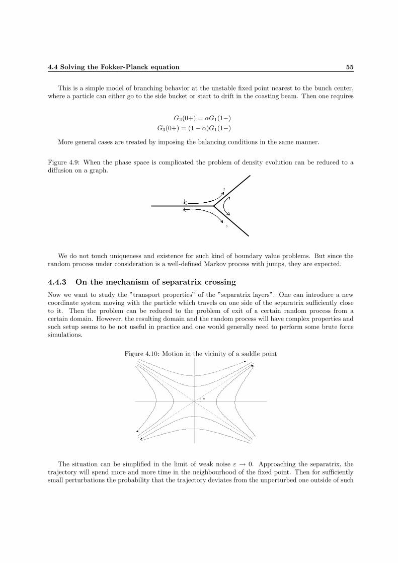
4.4 Solving the Fokker-Planck equation 55
This is a simple model of branching behavior at the unstable fixed point nearest to the bunch center,where a particle can either go to the side bucket or start to drift in the coasting beam. Then one requires
G2(0+) = αG1(1−)
G3(0+) = (1 − α)G1(1−)
More general cases are treated by imposing the balancing conditions in the same manner.
Figure 4.9: When the phase space is complicated the problem of density evolution can be reduced to adiffusion on a graph.
2
3
1
We do not touch uniqueness and existence for such kind of boundary value problems. But since therandom process under consideration is a well-defined Markov process with jumps, they are expected.
4.4.3 On the mechanism of separatrix crossing
Now we want to study the ”transport properties” of the ”separatrix layers”. One can introduce a newcoordinate system moving with the particle which travels on one side of the separatrix sufficiently closeto it. Then the problem can be reduced to the problem of exit of a certain random process from acertain domain. However, the resulting domain and the random process will have complex properties andsuch setup seems to be not useful in practice and one would generally need to perform some brute forcesimulations.
Figure 4.10: Motion in the vicinity of a saddle point
α
The situation can be simplified in the limit of weak noise ε → 0. Approaching the separatrix, thetrajectory will spend more and more time in the neighbourhood of the fixed point. Then for sufficientlysmall perturbations the probability that the trajectory deviates from the unperturbed one outside of such

56 RF noise
neighborhood is small and the whole effect of the perturbation will take place around the fixed point(see fig. 4.10). There the linear part of the equation dominates and one has a linear stochastic equationdescribing the motion sufficiently well. Then from the distribution of exit points from this neighborhoodone will know the transition probabilities between the domains after crossing the separatrix. The diffusioncoefficient of the random process will have some singularity due to divergence of trajectories going ondifferent sides of the separatrix. This makes the analytical treatment difficult 4. But the numerical studyof the linear system is trivial. Unlike for the nonlinear case, one can with a linear transformation arriveat a system with no small parameters and easily simulate the distribution of exit points.
Consider the linear system
φ = p+ εξ1(t)
p = λφ(1 + εξ2(t))
which after transformation p = p√λ, φ = φ becomes
˙φ =
√λp+ εξ1(t)
˙p =√λφ(1 + εξ2(t))
The sample paths of the system are shown in figure 4.11. One can immediately see the qualitativeinfluence of the separatrix slope
√λ on the dynamics of the random motion. The influence of the phase
noise ξ1 increases as λ → 0 and drops as λ → ∞. The amplitude noise ξ2 acts in the same manner, butthe time it has for its action growths as 1√
λ. The most probable displacement of a random process is along
the drift and against the gradient of the diffusion. The drift is given by the trajectories in figure 4.10, thediffusion gradient is zero for phase noise and upwards for amplitude. So, by stretching the trajectoriesof the unperturbed motion ”vertically” or ”horizontally” one gets the enhancement of the amplitude andphase noise correspondingly. This is the geometrical meaning of the slope
√λ. These considerations lead
to the conclusion that the increase of the slope leads to larger escape rate to the domains D1 and D3
under influence of both noise species. Such behavior is a consequence of the fact that it is easier to getout of the steep potential well.
In practice the particular escape rates can be estimated numerically. An example of the histogram ofexit domain distribution is shown in figure 4.12. This distribution depends weakly on the changes of theslope. A slight change can be observed when the main voltage is changed considerably, but small changeslike that introduced by the second RF system have no influence.
It has to be understood that the linearized system even when solved precisely would introduce somesmall error in the escape rate. But it can give
4.4.4 On numerical solution of the coupled system
As we have seen, analytical methods of solution fail even in the case of a two-point boundary value problemwhen the coefficients are sufficiently ”bad”. In case of the system of equations with coupled boundaryvalues the situation can become only worse. To obtain a solution numerical methods must be employed.We have tried several methods:
1. Algorithms based on Laplace transform [6]. Let u(t) be a real-valued function, then its Laplacetransform is given by
v(s) = L[u; s] =
∫ ∞
0
e−stu(t)dt (4.97)
4An asymptotic expansion was attempted by the author, but did not give satisfactory results. Further study is required.
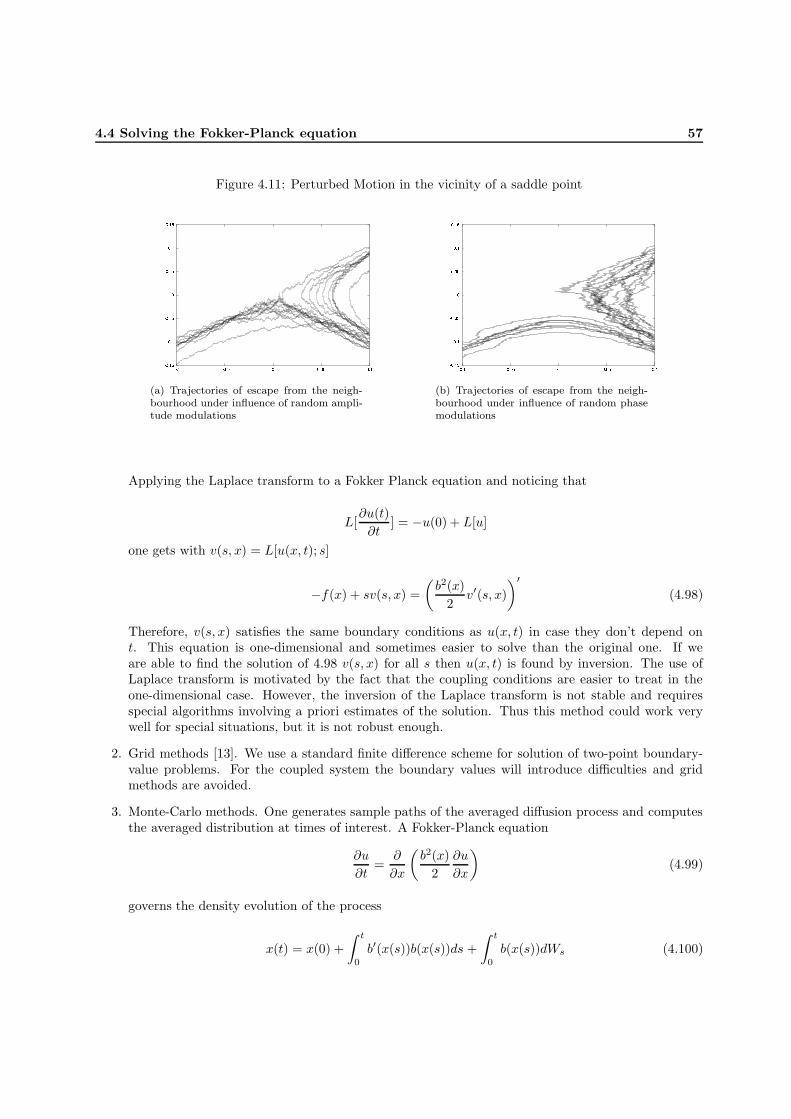
4.4 Solving the Fokker-Planck equation 57
Figure 4.11: Perturbed Motion in the vicinity of a saddle point
(a) Trajectories of escape from the neigh-bourhood under influence of random ampli-tude modulations
(b) Trajectories of escape from the neigh-bourhood under influence of random phasemodulations
Applying the Laplace transform to a Fokker Planck equation and noticing that
L[∂u(t)
∂t] = −u(0) + L[u]
one gets with v(s, x) = L[u(x, t); s]
−f(x) + sv(s, x) =
(
b2(x)
2v′(s, x)
)′(4.98)
Therefore, v(s, x) satisfies the same boundary conditions as u(x, t) in case they don’t depend ont. This equation is one-dimensional and sometimes easier to solve than the original one. If weare able to find the solution of 4.98 v(s, x) for all s then u(x, t) is found by inversion. The use ofLaplace transform is motivated by the fact that the coupling conditions are easier to treat in theone-dimensional case. However, the inversion of the Laplace transform is not stable and requiresspecial algorithms involving a priori estimates of the solution. Thus this method could work verywell for special situations, but it is not robust enough.
2. Grid methods [13]. We use a standard finite difference scheme for solution of two-point boundary-value problems. For the coupled system the boundary values will introduce difficulties and gridmethods are avoided.
3. Monte-Carlo methods. One generates sample paths of the averaged diffusion process and computesthe averaged distribution at times of interest. A Fokker-Planck equation
∂u
∂t=
∂
∂x
(
b2(x)
2
∂u
∂x
)
(4.99)
governs the density evolution of the process
x(t) = x(0) +
∫ t
0
b′(x(s))b(x(s))ds +
∫ t
0
b(x(s))dWs (4.100)

58 RF noise
Figure 4.12: A sample histogram of distribution of exit domains from the vicinity of a unstable fixed point
1 2 30
0.1
0.2
0.3
0.4
0.5
0.6
0.7
D1
D4
D2 and D3
(a) Amplitude noise
0.5 1.5 2.5 3.50
0.1
0.2
0.3
0.4
0.5
0.6
0.7
D1
D4
D2 and D3
(b) Phase noise
For small h the increment x(t+h)−x(t) is approximately normally distributed with mean b(x(t))b′(x(t))hand variance b(x(t))h. A straightforward application of this fact together with treating absorptionsand reflections leads to a Monte-Carlo algorithm. Two issues are important for implementation.First, to obtain a correct treatment of reflections, absorptions and to accurately represent the paths,one should have
h ∼∣
∣b2(x)∣
∣
∣
∣b′2(x)∣
∣
√N
(4.101)
Another difficulty is connected with the singularity (vanishing) of the coefficients. The flux throughsuch singular point is zero, no path can reach it, but this condition does not need to hold forapproximation with 4.100. Such situation is shown in figure 4.13. Here the flux 0.5b2(x)u′(x) atpoint 0 (bunch center) is zero,this condition is always satisfied for a bounded density due to vanishingcoefficient b2(0) = 0. The Monte-Carlo algorithm however ”does not know” about the singularitysince the trials are made for some neighbouring points with x 6= 0 , and finds a solution withvanishing derivative. This solution will have larger escape rate from the vicinity of a singular pointthan in reality. The error vanishes as the number of trials is increased, but due to this fact theconvergence of the method for singular coefficients is substantially slower.
One should also take care of the random number generator. Normally one uses simple formulae like
x =√
−2 log(u) sin(2πv) (4.102)
with u and v uniformly distributed random numbers. Since uniform random variables are generatedwith fast recurrent arithmetical methods, this will work rather fast. But the numbers thus generatedhave a cutoff. This introduces a small error and makes analysis of extreme paths difficult.
Monte-Carlo methods have poor convergence, but are robust and simple to implement. They aregood for rough estimate of complex system behavior, but are rarely useful when high precision isrequired. The estimation of the coasting beam population does not require such precision and withmodern computers the performance is acceptable.

4.5 Impact on synchrotron motion 59
Figure 4.13: Derivative error at a singular point
0 0.1 0.2 0.3 0.4 0.5 0.6 0.7 0.8 0.9 10
1
2
x
u(x)
finite difference solutionwith high precision
Monte−Carlo solution withinsufficiently small time step
x=0 is a singular point
4.5 Impact on synchrotron motion
4.5.1 Bunch diffusion - rough estimates
To estimate the diffusion of particles in the bunch core it is sufficient to take only few terms in the diffusioncoefficient representation. Under assumption that phase and amplitude noise are uncorrelated
b2(H) = b2phase(H) + b2ampl(H) . (4.103)
The first order expansion of the synchrotron oscillations in H gives
φ(t) =√H
√
2
K1sin(ωt)
p(t) =√H
√
2ω2
K1K23
cos(ωt)
K1 =qU
ET
K3 =2πhα
T
ω = K1K3 −1
4K3H (4.104)
If we are not interested in the effects produced by the form of the spectral density, we can drop thesynchrotron frequency shift and assume that the perturbation is white noise with intensity ε. Then
b2phase(H) =1
4ε2H (4.105)

60 RF noise
b2ampl(H) =1
8ε2H2ω2 . (4.106)
The amplitude noise has much more influence on the tails of the bunch than on the core. Somenumerical examples with exponential initial distribution and zero boundary value at some Hmax are shownin figure 4.14. In practice such a considerable change in the distribution over the time scale of beam storagecan be only possible when the noise is very strong. Usually a much weaker effect is observed.
The first order approximation can be used to describe the bunch core diffusion whereas for tail evolutionand the escape rate problem higher order terms should be employed as well as the proper boundaryconditions imposed.
4.5.2 Escape from the stable bucket
To assess the escape rate and to determine the ratio between loss and halo population more accuraterepresentation of the diffusion coefficient as well as the calculation of the distribution of escape domainsis required. An example of calculations with exaggerated noise level is shown in figure 4.15 and 4.16.
4.5.3 On effects of noise spectral density
Under the assumption that the noises are second order random processes one arrives at a substantialdependency of the results on the form of the spectral density. For systems with amplitude dependentfrequencies this may lead to a rather arbitrary behavior, i.e. one can adjust the spectrum so that the dif-fusion coefficient of the averaged system will have arbitrary form at least to some extent. The synchrotronoscillations usually lie within a rather narrow bandwidth (f.e. 0-30 Hz for HERA) and the spectrum ofoscillations is rather broad-band, so in reality this possibility is restricted. It can be easily shown that thederivative of the diffusion coefficient is bounded by the quantity of order ∂ω
∂H∂S∂ω where ω is the synchrotron
frequency and S is the spectral density of the random perturbation. But the measured spectral densitiesstill have a noticeable gradient. A qualitative example of two quite similar spectral densities and diffusioncoefficients derived from them is shown in figure 4.17. If the spectral density is allowed to be more irregularthen even larger divergence can occur. It should illustrate the fact that estimating the diffusion in thebeam tail is a subtle issue unless the spectral density is known quite precisely.
Adding the second RF system does not qualitatively change the behavior inside the buckets. There itresults only in a slight shift of the synchrotron frequency. But for the gap between the inner and outerbuckets (domain D4 in figure 4.5) the motion becomes more irregular (see figure 4.18). The oscillationspectrum includes more higher order harmonics. This means that the noise spectral density at these higherharmonics and their multiples will contribute to the diffusion coefficient.
The synchrotron oscillations spectrum in the beam tail D4 coming from the second RF system differsfrom the spectrum in the beam tail without the second system, this can influence the tail diffusion anddecide between the formation of bunch tail or the coasting beam. The estimation of this effect is againrestricted by the precision of knowledge of the noise spectral density.
4.5.4 Estimates for HERA
A measurement of the cavity voltage fluctuations is not trivial. An attempt to perform such measurementsfor phase noise at HERA was made [33]. It indicates that there is a possibility that the spectral densityis such that the diffusion coefficient at lower synchrotron frequencies is somewhat larger that at the high(figure 4.19). For such a spectrum shape the peaks turn out to be harmonics of the synchrotron frequencyof some tail particles, but not of the core. However, the relation of the measured noise to the actualvoltage fluctuation during a run is not obvious. The phase noise is usually more likely to appear due to
4.5 Impact on synchrotron motion 61
the complexity of the phase control system. The amplitude is normally generated with a better precisionand its fluctuations are usually neglected.
We were not aiming at precise estimates of the bunch diffusion. We suspect that the error in themeasurements of the noise spectrum might be considerable enough and definite conclusions cannot bedrawn. Even if it is not so, this problem requires a separate investigation and falls out of the scope ofthis work.5 The main goal is to show which impact the double RF system can have on the escape fromthe bucket and halo formation. The simulations were performed for noise spectra consistent with themeasurements [33] for the phase noise.
Due to the mentioned difficulties the simulations have a somewhat qualitative nature. They indicatethat under certain circumstances the accumulation of noticeable bunch tails in the side buckets is possible.It appears that particles can drift into their centers and accumulate there. The coasting beam itself isalso produced with a higher rate, but is then naturally cleaned by the synchrotron radiation mechanism.The halo corresponding to the ”gap” (domain D4) does not usually build up. For details see figures 4.20and 4.21.
5More careful measurements and analysis are planned at the moment.
62 RF noise
4.6 Summary
• The synchrotron tune spread is responsible for turning random coherent perturbations into randomincoherent ones. Without synchrotron tune spread it could be possible to reduce the effect of theRF noise by feedback. But it could hardly have any practical use.
• Both the bunch dilution and the escape rate from the RF bucket can be estimated provided thespectral density of the noise is known. Its incomplete knowledge introduces a substantial uncertaintyin the expected escape rate as well as in the entire bunch density evolution.
• Noticeable influence on the core may be produced by the phase noise. Amplitude noise has muchmore impact on the tails than on the bunch core.
• The second RF voltage introduces a region where a broader region of the noise spectral densityinfluences the motion, this can lead to diffusion enhancement in the bunch tails or halo formation.
• The RF noise can be well responsible for the coasting beam production by sweeping away the bunchtails.

4.6 Summary 63
Figure 4.14: Examples of density evolution of the synchrotron invariant under influence of phase andamplitude noise for some model parameters. Distributions are shown for t = 0h, t = 1h and t = 2h
0 0.1 0.2 0.3 0.4 0.5 0.6 0.7 0.8 0.9 10
0.1
0.2
0.3
0.4
0.5
0.6
0.7
0.8
0.9
1
H
f(H
)
0 0.1 0.2 0.3 0.4 0.5 0.6 0.7 0.8 0.9 10
0.1
0.2
0.3
0.4
0.5
0.6
0.7
0.8
0.9
1
Hf(
H)
(c) Phase noise, probability distribution u(H)
0 0.1 0.2 0.3 0.4 0.5 0.6 0.7 0.8 0.9 10
0.1
0.2
0.3
0.4
0.5
0.6
0.7
0.8
0.9
1
H
f(H
)
0 0.1 0.2 0.3 0.4 0.5 0.6 0.7 0.8 0.9 10
0.1
0.2
0.3
0.4
0.5
0.6
0.7
0.8
0.9
1
H
f(H
)
(f) Amplitude noise, probability distribution u(H)
0 0.1 0.2 0.3 0.4 0.5 0.6 0.7 0.8 0.9 10
0.1
0.2
0.3
0.4
0.5
0.6
0.7
0.8
0.9
1
H
f(H
)
0 0.1 0.2 0.3 0.4 0.5 0.6 0.7 0.8 0.9 10
0.1
0.2
0.3
0.4
0.5
0.6
0.7
0.8
0.9
1
H
f(H
)
(i) Phase and amplitude noise, probability distribution u(H)

64 RF noise
Figure 4.15: An exaggerated example of bunch density and halo evolution 1
(a) Diffusion coefficient (b) Loss rate
0
1
2
3
4
5
6
7
8
9
10
0 0.2 0.4 0.6 0.8 1
(c) Bunch core (distribution of synchrotron in-variant). Distributions at t = 0h and t = 1h
0
0.005
0.01
0.015
0.02
0.025
0 0.1 0.2 0.3 0.4 0.5 0.6 0.7 0.8 0.9 1
(d) Side bucket Halo

4.6 Summary 65
Figure 4.16: An exaggerated example of bunch density and halo evolution 2
(a) Diffusion coefficient (b) Loss rate
0
2
4
6
8
10
0 0.2 0.4 0.6 0.8 1
(c) Bunch core (distribution of synchrotron in-variant). Distributions at t = 0h and t = 1h
0
0.005
0.01
0.015
0.02
0.025
0 0.1 0.2 0.3 0.4 0.5 0.6 0.7 0.8 0.9 1
(d) Side bucket Halo

66 RF noise
Figure 4.17: Two spectral densities and diffusion coefficients obtained from them
(a) S1, 12/Hz (b) D1
(c) S2, 12/Hz (d) D2
Figure 4.18: Spectrum of the synchrotron oscillations in the gap between inner and outer buckets
0 10 20 30 40 50 60 70ω
(a) Phase
0 10 20 30 40 50 60 70ω
(b) Momentum
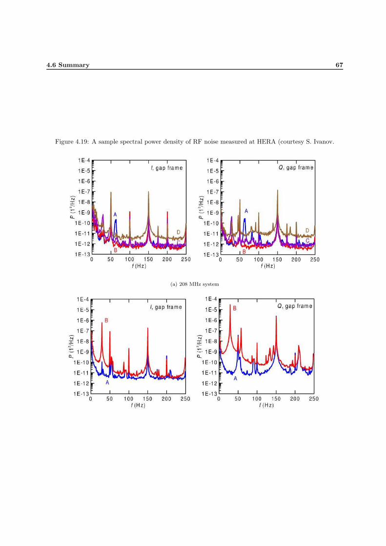
4.6 Summary 67
Figure 4.19: A sample spectral power density of RF noise measured at HERA (courtesy S. Ivanov.
(a) 208 MHz system

68 RF noise
Figure 4.20: Example of dynamics for HERA double RF system
(a) Density (b) Side bucket halo
(c) ”gap” halo (d) Loss, % vs. time

4.6 Summary 69
Figure 4.21: Another example with initially somewhat shorter bunches
(a) Density (b) Side bucket halo
(c) ”gap” halo (d) Loss, % vs. time

70 RF noise

Chapter 5
Some experimental observations
In this section we present the observed longitudinal bunch evolution in HERA and its connection tobackground rates. Perturbations can not only lead to parasitic losses but can also be employed for varioususeful purposes. We shortly discuss how RF voltage modulations can be employed to depopulate bunchtails and to achieve stabilization of multibunch oscillations.
5.1 Backgrounds and longitudinal bunch evolution
In HERA the longitudinal bunch profile is measured by analysing the current picked up from a resistivegap monitor. There are two systems. The first one is designed to measure the bunch distribution withrelatively high accuracy. It has a dead-time of around one second and cannot detect fast bunch oscillations.The second [65] has short dead-time and can measure bunch signal each turn, but the resolution is lowand it is used for analysis of fast bunch dipole oscillation modes and lengthening. A typical bunch profileevolution is shown in figure 5.1. The current in bunch tails is low and the measurement of its distributionis not possible due to limited resolution of the monitor. However, the amount of coasting beam can beassessed by measuring the difference between the bunched and unbunched (DC) current. The amount ofcoasting beam was also estimated by measuring the scattering rate at HERA-B target wires that weremoved across the beam [19].
Figure 5.1: Typical longitudinal bunch profile at HERA after the ramp and after a 10 hours run
The proton background is measured with counters installed in the detectors. The background ratesare also correlated with the loss rates measured at the collimators and with values taken from the beamloss monitors.

72 Some experimental observations
Figure 5.2: ZEUS C5 Counter with high background rates
Figure 5.3: ZEUS C5 Counter with moderate background rates
The background increases during the run which is explained by the proton halo accumulation. Byremoving a bad cable connection it was possible to improve the noise level in the RF system whichresulted in a considerable background reduction. In figures 5.2 and 5.3 the rates before and after theimprovement are shown.
The increase of the coasting beam with time under poor noise conditions is shown in figure 5.4, withbetter conditions - in figure 5.5.
Figure 5.4: Large coasting beam accumulation
The comparison of the observed coasting beam currents under improved noise conditions with sim-ulations is shown in figure 5.6. For the intra-beam scattering a slight overestimates is given. For thenoise the rates are show for various possible tail diffusion coefficients. To gain consistence of the bunchdiffusion with escape rate a significant increase of the coefficient towards the tail is to be assumed, whichwas suggested in [32].

5.2 Bunch manipulations with amplitude and phase modulations 73
Figure 5.5: Moderate coasting beam accumulation
Figure 5.6: Comparison of observed and simulated coasting beam currents
(a) Intra-beam scattering (b) Various levels of RF (phase) noise
5.2 Bunch manipulations with amplitude and phase modulations
By manipulating cavity voltage amplitudes and phases one can control to some extent the longitudinalbeam parameters. Such techniques are widely used to damp the longitudinal instabilities which can occurduring the ramp. By applying specific modulations one can influence particular parts of the beam, forexample depopulate the beam tail. With such technique one can in principle reduce the amount of thecoasting beam.
As was shown in Chapter 4, the diffusion coefficient arising from RF noise depends on its spectral den-sity. That means that by applying noise with spectral density concentrated in the synchrotron frequencyband of the bunch tail one can destroy the tail without influencing the longitudinal emittance considerably.The particles swept from the tail will mostly go into the coasting beam and will produce a backgroundincrease within some time. But since after such modulation the loss rate from the bucket should decreasewhichever loss mechanism is present, there would be a decrease in the background afterwards. An alter-native technique is based on the fact that amplitude noise results in the diffusion coefficient that growstowards the bunch tails. The amplitude modulation can now be made with a rather broad frequencyband, which will have approximately the same effect. Say, a white noise can be used.
We attempted an experimental confirmation of this facts. Synchrotron frequencies of tail particlesin HERA are around 1 Hz and voltage modulation of this frequencies turned to be technically difficult.We applied white noise instead. The noise signal with amplitude of 1 kV was applied to the cavity for10 minutes. The collimator rates were observed. The applied noise resulted in a slight collimator rate

74 Some experimental observations
increase and had no influence on the bunch core. After 1 hour the collimator rates increased significantly.The time interval corresponds to the time required for the particles pulled out from the tail to drift to theaperture limitation under influence of synchrotron radiation. After that the backgrounds decreased andwere lower than those which should have been without the perturbation. A usual background evolutionis shown in figure 5.8. The backgrounds observed after the amplitude modulation is shown in figure 5.7.A decrease in the coasting beam production was also observed (figure 5.9). 1
Figure 5.7: Collimator rates after the amplitude modulation. The modulation was applied at ∆t ≈ 0.7h
Figure 5.8: Usual picture of the collimator rates on the same time scale
Figure 5.9: Coasting beam current after the amplitude modulation. The increase in the accumulation ratecorresponds to the time of the modulation.
1the coasting beam currents have different orders because of the different number of stored bunches. Low beam currentwas used for safety reasons.

5.3 Summary 75
Figure 5.10: Usual coasting beam accumulation observed on the same time scale goes linearly.
5.3 Summary
• There is some portion of coasting beam coming from the intra-beam scattering. For a proton ringlike HERA it shouldn’t have a serious background impact.
• Most of the halo seems to be accumulated due to the RF phase noise.
• It is hard to practically reduce further the noise level at HERA.
• Random perturbations can be used for beam control.

76 Some experimental observations

Chapter 6
Epilogue
6.1 Noise in nonlinear systems
The distinction between random and deterministic processes is rather subtle from the modern point ofview. It is long known [14] that complex dynamical systems possess statistical properties. A randomprocess can be viewed as an output of a chaotic dynamical system. One can consider a perturbation tobe deterministic if it has a regular Fourier spectrum.
Such deterministic perturbations of the synchrotron motion arise as a consequence of wake fieldsproduced by the bunch train travelling in the ring, higher order harmonics of the RF cavities and so on.A periodic driving of a linear system can result in resonant behavior and an instability can occur. For anonlinear Hamiltonian system where frequency depends on the amplitude another behavior, the so callednonlinear resonance, is general [12]. A perturbation results in a set of points (or hypersurfaces) in thephase space where the resonant conditions are met. The perturbation has a strong effect in the vicinity ofthese points leaving the motion in all other regions practically unchanged. The region where the impactis strong is called the resonant band. Since such points generally form a dense set in the phase space,the effect of intersection of different resonant bands can be rather complicated. For a certain class ofsystems - steep Hamiltonian systems - a sufficiently small perturbation does not lead to instability. Inone-dimensional case these systems are just Hamiltonian systems with positively definite Hamiltonian.Such is, for example, the pendulum representing the synchrotron oscillations. For such Hamiltoniansmotion along every resonant line introduces a frequency shift and the perturbation is thus stabilized.These issues are of great importance for the transverse beam dynamics where all kinds of resonances canappear due to multidimensionality [62], [59].
A general description of dynamics when nonlinear resonances are present is extremely complicated[12]. The situation becomes more difficult when a random force is added. Many interesting physicalphenomena arise, especially in systems with multiple stable points or lattice systems - pattern formation,stochastic resonance, etc. (see for example [67], [23]). For Hamiltonian systems a rich variety of resultscan be drawn from simple models, for example from interaction of an isolated resonances with white noise[25], [57]. Here the phase space topology created by the nonlinearity introduces “channels” which hostcirculations of currents driven by noise. This behavior can strongly influence stationary distributions andvarious escape rates.
For one dimensional systems the behavior is much simpler. A resonant surface reduces to a point inthe action space with trajectories oscillating around this point, an isolated resonance. An instability canoccur when the isolated resonances intersect each other and this intersection is broad enough to providean escape path to the trajectory. This effect is normally small for reasonably weak perturbations arising inthe synchrotron motion which can be suspected to contribute to escape rate from the RF bucket. However,

78 Epilogue
it is not completely excluded. Another instability mechanism could come from the possibility of quicktransport of a particle across a resonant band which in interaction with the noise can lead to a diffusionenhancement.
The discussed effects play much weaker role in the one dimensional case than in multidimensional.Therefore, it is as usual hard to estimate the perturbations experimentally due to their small magnitudes.However, this mechanisms are to be kept in mind. Note that the interaction with a resonance is to someextent already included in the Fokker-Planck equation obtained from the given spectral power density.Any perturbation acting in a physical device in reality has some bandwidth.A peak measured in the outputof some device can be viewed as the spectral power density at this point. Then the diffusion coefficient4.20 in the region with corresponding frequency spread will grow as well. The numerical correspondenceof the diffusion rate to the reality is of course not that obvious. The description becomes somewhat looseas the bandwidth goes to zero and the peak becomes sharper. Then the influence of this peak from therandom process point of view shrinks to a diffusion in a small region whereas in reality there should exista certain resonant band with some “quasiregular” motion in it. So, sharp narrow peaks of high intensityin the noise should be rather considered as deterministic components.
6.2 Conclusion
The loss rates for HERA were estimated when intra-beam scattering and RF noise are present. Theinfluence of intra-beam scattering turned out to be weak. The RF noise appears to be responsible forthe major portion of the coasting beam. These values were estimated to a precision which is determinedby the error in the measurement of the noise spectral density. The estimates of noise in this work havemainly of qualitative nature.
The discussed methods can be potentially applied to some other problems concerning random particlemotion and backgrounds which can appear in connection with the coming operation of the LHC and,possibly, other accelerators.
Substantial complications arise in extending the methods to general multidimensional nonlinear sys-tems where chaotic behavior can take place. The averaging becomes not trivial, the numerical integrationand Monte-Carlo trials require much more computations.
Another difficulty in the study of random phenomena is the selection of a correct noise model. Conven-tional models are presented by the second order processes or by white noise. However, there is a varietyof situations when they cannot be used [24].
The problem of escape from the potential well under influence of random perturbations has no generalelegant solution. It has been widely studied in particle accelerator theory and in connection to otherproblems. For particular applications one can normally achieve a satisfactory solution by combininganalytical and numerical methods and exploiting the specific properties of the system. The demonstrationof such methods for the problem of escape from the RF potential bucket in a storage ring was attemptedin this work. We hope that at least some ideas have a shade of originality at least for the acceleratorcommunity.

Appendix A
Particle motion in a storage ring
A.1 Equations of motion
The horizontal and vertical coordinates of a particle are measured in a Cartesian coordinate system movingalong the design orbit
r(s) =
x(s)x′(s)z(s)z′(s)
They are sums of the coordinates of the closed orbit for a given momentum deviation ∆p and thecoordinates of betatron oscillations around the closed orbit
rβ(s) =
xβ(s)x′β(s)zβ(s)z′β(s)
r(s) = rβ(s) +D(s)∆p
p(A.1)
The betatron motion can be represented by a certain coordinate map
rβ(s+ L) = M(s+ L, s)rβ(s) (A.2)
When all nonlinear elements are taken into account, M becomes a complex nonlinear map. However,for applications like intra-beam scattering linear optics approximation is sufficient. Neglecting the couplingbetween the transverse planes and nonlinear effects, M becomes a matrix expressed in terms of the opticalfunctions (linear optics)
M(s+ L, s) =
(
Mx(sL, s) 00 My(s+ L, s)
)
Mx,y(s+ L, s) =
√
βx,y(s+L)βx,y(s) (cos(Ψx,y) + α(s) sin(Ψx,y))
√
βx,y(s+ L)βx,y(s) sin(Ψx,y)
(αx,y(s)−αx,y(s+L)) cos(Ψx,y)−(1+αx,y(s)αx,y(s+L)) sin(Ψx,y)√βx,y(s)βx,y(s+L)
√
βx,y(s)βx,y(s+L) (cos(Ψx,y) − αx,y(s) sin(Ψx,y))

80 Particle motion in a storage ring
or explicitly
rβ,x,y =√ε√
β (cosΨ cosφ− sin Ψ sinφ)
rβ,x′,y′ = −√
ε
β(α cosΨ cosφ− α sin Ψ sinφ+ sin Ψ cosφ+ cosΨ sinφ)
cosφ =rβ,0εβ0
sinφ = − 1√ε
(
rβ,0√
β0 +α0rβ,0√β0
)
(A.3)
Here βx,z is the betatron envelope function, αx,z = −β′x,z
2 , Ψx,z is the betatron phase.The matrix Mis symplectic and the transformation preserves area in the phase space. Normalized invariant phase spaceareas of this transformation are the emittances
εx =1 + α2
x(s)
βx(s)x2(s) + 2αx(s)x(s)x
′(s) + βx(s)x′2(s) (A.4)
εz =1 + α2
z(s)
βz(s)z2(s) + 2αz(s)z(s)z
′(s) + βz(s)z′2(s) (A.5)
Due to phase focusing particles perform slow synchrotron oscillations. Let the reference energy be E,the energy offset ∆E, the synchrotron phase φ, then the synchrotron one turn map is given by
∆En+1 = ∆En + eZV (φ) − ∆Eγ
φn+1 = φn +2πh
β2E
(
α− 1
γ2
)
∆E
This map is approximated with a system of differential equations
∆E =eZ
TV (φ) − ∆Eγ
T
φ =2πh
β2ET
(
α− 1
γ2
)
∆E
where
α = ∆LL
p∆p − the momentum compaction factor,
V (φ) − RF voltage,β, γ − relativistic factors,h = ωRF
ωREV− harmonic number,
E − reference energy,q = eZ − particle charge,∆Eγ − energy change from synchrotron radiation,T − revolution period
SinceE2
c2= p2 +m2c2 (A.6)

A.1 Equations of motion 81
and for ultrarelativistic particles
δp =∆p
p=
∆E
E(A.7)
the equations of motion can be rewritten
δp =eZ
TEV (φ) − ∆Eγ
ET
φ =2πh
β2T
(
α− 1
γ2
)
δp
The spacial longitudinal coordinate with respect to bunch centre is more convenient in kinetic equationsand is related to the phase as
∆s =cφ
2πωRF(A.8)
The synchrotron radiation is emitted with mean power
Pγ =e2c
6πε0
γ4
R2(A.9)
where ε0 = 8.8× 10⁻¹²farad×m−1 is the permittivity in vacuum. The fluctuations of the power due toquantum nature of the radiation are negligible for proton storage rings. The energy losses per turn are
∆E = c∆p =
∫ T
0
Pγdt ≈Te2c
6πε0
γ4
R2(A.10)
In the case of stable synchrotron oscillations the radiation losses are compensated by the Rf systemand the change of δp is given by the difference in the radiation losses with respect to the reference particle
∆Eγ = T∂Pγ∂E
∆E =4
γm0cPγ∆E (A.11)
When the motion is not oscillatory the energy losses are not compensated and
∆Eγ = TPγ (A.12)
For example, for protons in HERA the synchrotron oscillation damping rate is of order 1KeV/secand the damping time is tens of days. The drift is about 280KeV/sec, the time required to drift fromthe bucket to the acceptance limit is about 40min. So, for the time scales involved, one can neglect theradiation damping for oscillating particles, but the drift in the coasting beam region is substantial andcontributes to particle losses.
The radiation effects and all other perturbations are rather week and can be considered as smallperturbations to the Hamiltonian system with
H(φ, δp) =q
TU(φ) +
2πh
β2T
(
α− 1
γ2
)
δp2
2(A.13)
where −U ′(φ) = V (φ). For the case of sinusoidal RF voltage V (φ) = sin(φ) the Hamiltonian is
H1(φ, δp) =q
ET(1 − cos(φ)) +
2πh
β2T
(
α− 1
γ2
)
δp2
2(A.14)

82 Particle motion in a storage ring
For the double RF system one takes the phase with respect to one of the systems (the dominant) asφ and supposing ωRF2 = η · ωRF1
H2(φ, δp) =q
ET(2 − V1 cos(φ) − V2 cos(ηφ)) +
2πh
β2T
(
α− 1
γ2
)
δp2
2(A.15)
The part of the Hamiltonian depending on φ is called the RF potential. In figures A.2 and A.3 theRF potentials and phase portraits of systems A.14 and A.15 are shown. System A.14 has fixed points
φ = 0, ±π2, ±π
The fixed points of system A.15 can be found to a good accuracy as corrections to single RF fixedpoints. To the first order the correction is zero and can be neglected when cavities voltages differ much.
Some parameters for HERA are summarized in table A.1.
Table A.1: Some HERA parametersFirst RF system frequency ωRF1 208MHz
Second RF system frequency ωRF2 52MHzRF voltage U ∼ 500KV
Synchrotron frequency ω ∼ 30HzMomentum compaction α = 0.00128
Averaged optical functions 〈βx〉 = 100m, 〈βz〉 = 80m〈αx〉 = 7.4 × 10⁻⁶, 〈αz〉 = 1.7 × 10⁻⁴
〈Dx〉 = 1.06m, 〈Dy〉 = 0.002m
The momentum acceptance is the maximum momentum offset that a particle can have without beinglost transversely. For HERA the δp/p acceptance is about 10−3 (at 920 GeV, with U208 = 360KV andU52 = 14KV ).
A.2 Action-angle variables
To analyze the long term stability of motion one normally looks at the behavior of some slowly varyingquantities or invariants of motion. It is convenient to study weekly perturbed Hamiltonian systems interms of action-angle variables of the unperturbed systems. A Hamiltonian can be brought by a canonicaltransformation of variables (q, p) → (J, φ) to the form H(J). If the system is integrable (which is alwaystrue for 1d Hamiltonian systems) then such action-angle transformation can always be made. In action-angle variables the equation of motion takes the form
J = 0
φ = ω(J) = −∂H∂J
(A.16)
This transformation to action-angle variables sometimes can be found explicitly. For example, for thependulum
H(q, p) =p2
2+ Ω(1 − cos q) (A.17)
such transformation is given by the Jacobi elliptic functions [5]. However, analytical representationsare exceptional and in practice one has to rely on an asymptotic expansion. A common perturbation

A.2 Action-angle variables 83
method to bring a Hamiltonian into action-angle form is the superconvergent method. Here it is shownfor a simple one-dimensional case. For the pendulum (with Ω = 1) the Hamiltonian can be representedas series
H =p2
2+q2
2− q4
4!+q6
6!− q8
8!+ . . . (A.18)
First J = q2
2 + p2
2 , q =√
2Jcosφ
H(J, φ) = J − 4J2
4!cos4 φ+
8J3
6!cos6 φ− 16J4
8!cos8 φ+ . . . (A.19)
Dividing the Hamiltonian into the mean and oscillating parts
H(J, φ) = J − 4J2
4!
⟨
cos4 φ⟩
+8J3
6!
⟨
cos6 φ⟩
− 16J4
8!
⟨
cos8 φ⟩
+
4J2
4!(cos4 φ−
⟨
cos4 φ⟩
) +8J3
6!(cos6 φ−
⟨
cos6 φ⟩
) − 16J4
8!(cos8 φ−
⟨
cos8 φ⟩
) + . . .
one chooses the next transformation to eliminate the oscillating terms of order J 2. One chooses thegenerating function
F (J1, φ) = J1φ+ S(J1, φ)
so that
J = J1 + Sφ
φ1 = φ+ SJ1
the desired transformation is obtained with
Sφ =1
6J2
1 (cos4(φ) − 3
8)
Then one needs to change φ → φ1 according to
φ1 = φ+ SJ1= φ+
∫
Sφ,J1dφ = φ− 8a4J1
∫
f4(φ)dφ + c(φ)
By the next transformation one can eliminate terms of order J 3 and J4. Up to fourth order this givesthe Hamiltonian
ˆH(J1) = J1 −J2
1
16− J3
1
256− 5J4
1
213(A.20)
Note that the expression obtained by averaging the Hamiltonian H(J) with respect to phase will differfrom H(J1)
〈H(J)〉 = J1 −J2
1
16− J3
1
288− 5J4
1
9216(A.21)
which differs noticeably in terms starting from fourth order. In many problems such averaging issufficient and one can use such first order action. Action-angle variables are standard in treating smallperturbations. Suppose that the original system was subject to a perturbation which is a smooth functionin q and p. Then in action-angle variables it is some smooth function of J and periodic in φ. The perturbedHamiltonian can be written in the standard form
H(J, φ) = H0(J) + ε∑
m,n
Vm,neiwmφ+iνnt (A.22)
With such a representation averaging and resonance analysis can be now more easily performed.

84 Particle motion in a storage ring
Figure A.1: Optical functions at HERA
0.0 1000. 2000. 3000. 4000. 5000. 6000. 7000. 8000.s (m)
δ E/ p 0c = 0 .0 0 0 0 0
Table name = TWISS
hpl920e+Unix version 8.51/13 29/07/04 13.48.06
0.0
200.
400.
600.
800.
1000.
1200.
1400.
1600.
1800.
βx(m
)
β x
(a) βx
0.0 1000. 2000. 3000. 4000. 5000. 6000. 7000. 8000.s (m)
δ E/ p 0c = 0 .0 0 0 0 0
Table name = TWISS
hpl920e+Unix version 8.51/13 29/07/04 13.48.06
-80.
-60.
-40.
-20.
0.0
20.
40.
60.
80.αx α x
(b) αx

A.2 Action-angle variables 85
Figure A.2: Synchrotron motion with 1 RF system
−4 −3 −2 −1 0 1 2 3 4φ
(a) Potential
−4 −3 −2 −1 0 1 2 3 4φ
(b) Phase space
Figure A.3: Synchrotron motion with 2 RF systems
−4 −3 −2 −1 0 1 2 3 4φ
(a) Potential
−2.5 −2 −1.5 −1 −0.5 0 0.5 1 1.5 2 2.5φ
(b) Phase space

86 Particle motion in a storage ring

Appendix B
Sketch of the proof of proposition 1
One needs to show that an integral of a random function along a trajectory of the solution of the differentialequation can be under certain conditions approximated on [0, T0] by an Ito’s integral
∫ τ
0
fε(p(ε−2s), φ(ε−2s), s)ds+
1
ε
∫ τ
0
gε(p(ε−2s), φ(ε−2s), s)ds ≈
∫ τ
0
a(H(s))ds+
∫ τ
0
b(H(s))dWs
Let p(t) and φ(t) be represented as functions of the invariant H and t, the problem can be restated as
∫ τ
0
fε(H(ε−2s), ε−2s)ds+1
ε
∫ τ
0
gε(H(ε−2s), ε−2s)ds ≈∫ τ
0
a(H(s))ds+
∫ τ
0
b(H(s))dWs (B.1)
The idea of the proof is that one can find such ∆ that is much greater than the correlation time ofthe random function so that the integral over [0,∆] becomes a sum of some large number of integralsthat are approximately independent random variables, but the change of H on such an interval is small.Then the increment of the process on this interval becomes approximately a Gaussian random variable.Its moments define the drift and diffusion coefficients of the diffusion process sought. Such ∆ can alwaysbe found for processes with finite correlation time and sufficiently small ε. Let the partition of [0, T0] onsuch intervals be constructed. First consider the term of second order in ε and develop it in power seriesto the second order around the starting point
∫ ∆
0
fε(H(ε−2τ), ε−2τ)dτ =∆
∆ε−2
∫ ∆ε−2
0
fε(H(τ), τ)dτ = (B.2)
∆ limT→∞
1
T
∫ T
0
fε(H(0), τ)dτ +O(∆2) (B.3)
The variation of the last integral is of order ∆2 and the first moment of order ∆. This means that itscontribution reduces to drift
limT→∞
1
T
∫ T
0
〈fε(H(0), τ)〉 dτ (B.4)
Extending this procedure to the whole interval one arrives at the drift coefficient

88 Sketch of the proof of proposition 1
a(H) = limT→∞
1
T
∫ T
0
〈fε(H, τ)〉 dτ (B.5)
Now consider the term of order ε
1
ε
∫ 1
0
gε(H(ε−2τ), ε−2τ)dτ =∆
ε · ε−2
∫ ∆ε−2
0
gε(H(τ), τ)dτ =
∆
ε · ε−2
∫ ∆ε−2
0
[
gε(H(0), τ) +∂gε∂H
(H(0), τ)
∫ τ
0
gε(H(0), s)ds
]
dτ +O(∆2)
The first moment of the last integral is
∆
εlimT→∞
1
T
∫ T
0
〈gε(H(0), τ)dτ〉 +∆
εlimT→∞
1
T
∫ T
0
dτ
∫ τ
0
⟨
∂gε∂H
(H(0), τ)gε(H(0), ε−2s)ds
⟩
+O(∆2) (B.6)
The first integral is large and contributes to the drift on faster time scales than ε−2, namely ε−1. Totreat the diffusion on time scale of ε−2 one first needs to transform the equation to variables in which itvanishes. However in our case (for the synchrotron motion) it turns out to be zero due to fast oscillationsin gε with zero mean and this is not required. So the drift comes from the second term. It can be rewrittenas
∆ limT→∞
1
T
∫ T
0
dτ
∫ τ
0
⟨
∂gε∂H
(H(0), τ)gε(H(0), ε−1s)ds
⟩
+O(∆2) =
∆ limT→∞
1
T
∫ T
0
dτ
∫ τ
0
⟨
∂gε∂H
(H(0), τ)gε(H(0), s)
⟩
ds+O(∆2)
When extending the integration procedure to the whole interval in the last expression the correlationsfrom the past have also to be taken into account. Neglecting terms of order ∆2 the drift becomes
limT→∞
1
T
∫ T
0
dτ
∫ τ
−T
⟨
∂gε∂H
(H, τ)gε(H, s)
⟩
ds (B.7)
The second variation of B.6 is
⟨
∆ · ∆ε2 · ∆ε−2 · ∆ε−2
∫ ∆ε−2
0
gε(H(0), τ1)dτ1
∫ ∆ε−2
0
gε(H(0), τ2)dτ2
⟩
+O(∆2) =
∆
⟨
1
∆ε−2
∫ ∆ε−2
0
gε(H(0), τ1)dτ1
∫ ∆ε−2
0
gε(H(0), τ2)dτ2
⟩
+O(∆2) =
(B.8)
and the diffusion coefficient
limT→∞
1
T
∫ T
0
∫ T
0
〈gε(H, τ1)gε(H, τ2)〉 dτ1dτ2 (B.9)
To complete the proof one needs to show that the correlation between consequent subintervals issmall compared to the first moments of the process and that on each interval the random perturbation

89
satisfies the central limit theorem with desired precision. It turns out that one should choose ∆ ∼ ε√ε to
satisfy these conditions. The magnitude of ∆ determines the precision of the approximation√ε. Precise
conditions under which the procedure is applicable can be found in [37], [28]. These conditions are metfor sufficiently small ε and a random process of second order with finite correlation time.
Note that for moderate noise amplitude it may turn out that such an averaging procedure may giveonly a poor approximation due to the square root convergence. In that case the non-Markovian nature ofnoise is essential and one has to deal with the system of Ito’s equation in the extended phase space [55].
The behavior of random oscillating systems on long time scales was also studied in [3], [4], [22], [38].

90 Sketch of the proof of proposition 1

Appendix C
On the precision of the’self-consistent chains’ method
The chain dynamics can be represented by a series of mappings (multiplications)
xτ = xT0 P (x0, τ), 0 ≤ τ ≤ h1
xτ = xTh1P (xh1
, τ), h1 ≤ τ ≤ h2
. . . . . . . . . . . .xτ = xThi
P (xhi, τ), hi ≤ τ ≤ hi+1
. . . . . . . . . . . .
(C.1)
where xτ are distribution vectors belonging to Rn, the transition probability matrix P (x, t) is some
function from Rn × R to R
n×n, P (x, 0) = E, and hi is a partition of the time interval [0, T ] with thepoints representing the moments of time at which the distribution is recalculated.
Let hi = ∆ · i = im , the case of an arbitrary partition is analogous. For this partition the system is
truncated at i =[
1∆
]
. Here we show some convergence estimates for such dynamical system.
Lemma 2 Let P (x, τ) possess smooth derivatives up to second order and bounded derivatives of higher
orders. Then for distributions xτ and yτ starting at initial distributions x0 and y0 there exists a constant
C not depending on ∆ such that ‖xτ − yτ‖ < Cε on τ ∈ [0, T ] whenever ‖x0 − y0‖ < ε.
Proof
Without loss of generality we may assume T = 1. Consider a partition with ∆ = 1m . Consider some
interval of the partition [hi, hi+1] and the evolution of the system with distributions at hi equal to xi andyi.
‖xi+1 − yi+1‖ =
∥
∥
∥
∥
xTi P (xi,1
m) − yTi P (yi,
1
m)
∥
∥
∥
∥
=
=
∥
∥
∥
∥
xTi P (xi,1
m) − yTi P (xi,
1
m) + yTi P (xi,
1
m) − yTi P (yi,
1
m)
∥
∥
∥
∥
≤
≤ ‖xi − yi‖∥
∥
∥
∥
P (xi,1
m)
∥
∥
∥
∥
+ ‖yi‖∥
∥
∥
∥
P (xi,1
m) − P (yi,
1
m)
∥
∥
∥
∥
For all finite dimensional distributions ‖x‖ ≤ 1 (in C or p norm), xTP is again a distribution and thus

92 On the precision of the ’self-consistent chains’ method
‖P‖ = sup‖x‖=1‖xTP‖‖x‖ ≤
∥
∥xTP∥
∥ ≤ 1. The previous inequality turns now to
‖xi+1 − yi+1‖ ≤ ‖xi − yi‖ +
∥
∥
∥
∥
P (xi,1
m) − P (yi,
1
m)
∥
∥
∥
∥
Develop P (yi, τ) in power series around τ = 0, then
‖P (xi, τ) − P (yi, τ)‖ ‖E + τPτ (xi, 0) +τ2
2Pτ2(xi, 0) + . . .−
− (E + τPτ (yi, 0) +τ2
2Pτ2(yi, 0) + . . .)‖
(C.2)
If Pτ is Lipschitz-continuous at zero, i.e. when
‖Pτ (x, 0) − Pτ (y, 0)‖ ≤ L ‖x− y‖
the last expression is of order τ ‖x− y‖ and for some bounded L
‖xi+1 − yi+1‖ ≤ ‖xi − yi‖(
1 + L1
m
)
From this follows that
‖xk − yk‖ ≤ ‖x0 − y0‖(
1 +L
m
)k
≤ ‖x0 − y0‖(
1 +L
m
)m
≤ ‖x0 − y0‖ eL
for all k ≤ m.
Lemma 3 For fixed n the sequence of functions xτ converges to some limit x?τ , which is a solution of
the system of nonlinear equations
x? = A(x?)
where
A(x) = limτ→0
P (x, τ) −E
τ
and ‖x− x?‖ ≤ Cm
Proof. Consider the evolution of xτ over interval [hi, hi+1]
xi+1 = xTi P (xi, τ), τ = hi+1 − hi
thenxi+1 − xi
τ= xTi
P (xi, τ) −E
τ
and going to the limitx? = x?TA(x?)
which is equivalent to
x?(t) = x?0 +
∫ t
t0
x?T (τ)A(x?(τ))dτ
xi+1 = xTi P (xi, τ) = xTi (E + Pτ (xi, 0) +O(τ2)) = xTi (E + τA(xi) +O(τ2))

93
x?(hi+1) − xi+1 = x?(hi) +
∫ hi+1
hi
x?(τ)P (x?(τ), τ)dτ − xi − τxTi A(xi) +O(τ2)
x(τ) = xi + τd
dτx(τ)τ=hi
+O(τ2)
A(x(τ)) = A(x?(hi) + τx?(hi)d
dxA(x?(hi)) +O(τ2)) = A(xi) + τ ˆA(xi) +O(τ2)
∫ hi+1
hi
x(τ)A(x(τ))dτ = xiA(xi)(hi+1 − hi) +O(hi+1 − hi)2 +O((hi+1 − hi) ‖xi − x?hi‖)
‖xi+1 − x?(hi+1)‖ ≤ ‖xi − x?(hi)‖ +M1(hi+1 − hi) ‖xi − x?(hi)‖ +M2(hi+1 − hi)2
or
‖xi+1 − x?(hi+1)‖ ≤ ‖xi − x?(hi)‖ (1 +M1
m) +
M2
m2
From this it follows that the upper bound of the error at point hi+1 must satisfy
δi+1 = δi(1 +M1
m) +
M2
m2, i = 1, . . .m
Since δi is an increasing function of i it is sufficient to estimate δm. Obviously δm cannot be smaller thanM2
m . This means that we should expect no better than a linear bound on δm. Choose some M ′ and choose
k so that δk−1 <M ′
m and δk ≥ M ′
m .Such k exists for all M ′ ≤M . Then M2
m2 ≤ δM2
M ′ and
δi+1 ≤ δi(1 +M1 +M2/M
′
m)
for all i > k.
δm ≤ δk+1(1 +M1 +M2/M
′
m)m−k−1 ≤ δk+1(1 +
M1 +M2/M′
m)m ≤ δk+1e
M1+M2/M′
Since δk <M ′
m δk+1 ≤ M ′
m (1 + M2
m ) + M2
m2
δm ≤ M ′
m(1 +
M2
m) +
M2
m2eM1+M2/M
′
The last expression attains a minimum at M ′ = M2. Altogether , the error can be majorated by C1
m + C2
m2
or by Cm .
We now have to show convergence of xnτ as n → ∞. To do that observe that the probability densityof a Markov jump process having sufficient regularity satisfies a linear integral equation
∂p(x, t)
∂t=
∫ ∞
−∞K(x, y)p(y)dy (C.3)
whereK(x, y) tells about the probability of a jump from point y to a neighbourhood of point x.Supposethere exists a finite or countable set Ω such that both initial distribution and the kernel of the integraloperator are concentrated at these points, then the solution of equation C.3 will be also concentrated inthese points. Then we can search for solutions in the form
94 On the precision of the ’self-consistent chains’ method
p(x, t) =∑
ω∈Ω
cω(t)δ(xω) (C.4)
the kernel is of the formK(x, y) =
∑
ω,ω′∈Ω
aωω′δ(xω) (C.5)
After substituting this into C.3 it splits into a system of ordinary differential equations for the coeffi-cients cn which is exactly the Kolmogorov system for a corresponding Markov chain.
cω(t) =∑
ω′∈Ω
aω,ω′cω′(t) (C.6)
Suppose that the sequence of kernelsKn converges (weakly) to a kernel K, which now doesn’t need to bea combination of delta-functions. Suppose that pn(x, t) and p(x, t) are solutions of eq. C.3 correspondingto kernels Kn and K. then they satisfy integral equations
pn(x, t) = pn(x, 0) +
∫ t
0
∫ ∞
−∞Kn(x, y)pn(y)dydt
and
p(x, t) = p(x, 0) +
∫ t
0
∫ ∞
−∞K(x, y)p(y)dydt
‖pn(x, t) − p(x, t)‖ =
=
∥
∥
∥
∥
pn(x, 0) − p(x, 0) +
∫ t
0
∫ ∞
−∞(Kn(x, y)pn(x, τ) − K(x, y)p(y, τ))dydt
∥
∥
∥
∥
≤
≤ ‖pn(x, 0) − p(x, 0)‖ +∥
∥
∥
∥
∫ t
0
∫ ∞
−∞(Kn(x, y)pn(x, τ) −Kn(x, y)p(y, τ) +Kn(x, y)p(y, τ) − K(x, y)p(y, τ))dydτ
∥
∥
∥
∥
≤
≤ ‖pn(x, 0) − p(x, 0)‖ +
∫ t
0
(‖Kn‖ ‖pn(x, τ) − p(x, τ)‖ +∥
∥
∥Kn − K
∥
∥
∥‖p(x, τ‖)dτ (C.7)
‖pn(x, t) − p(x, t)‖ ≤ ‖Kn‖∫ t
0
‖pn(x, τ) − p(x, τ‖ dτ + ‖p(x, t)‖∥
∥
∥Kn − K
∥
∥
∥t+ ‖pn(x, 0) − p(x, 0)‖
and noticing that ‖p‖ and ‖Kn‖ are bounded by 1
‖pn(x, t) − p(x, t)‖ ≤∫ t
0
‖pn(x, τ) − p(x, τ‖ dτ +∥
∥
∥Kn − K∥
∥
∥ t+ ‖pn(x, 0) − p(x, 0)‖
The Gronwall inequality says that whenever z(t) ≥ 0 and satisfies
z(t) ≤ c
∫ t
0
z(τ)dτ + b
thenz(t) ≤ bect
Applying this to the previous estimate with z(t) = ‖pn(x, t) − p(x, t)‖ +∥
∥
∥Kn − K∥
∥
∥ we arrive at

95
‖pn(x, t) − p(x, t)‖ ≤ ‖pn(x, 0) − p(x, 0)‖ et +∥
∥
∥Kn − K
∥
∥
∥(et − 1)
the estimate is valid for t < h1 , i.e in the interval when the process is Markov. The same reasoningcan be applied to consequent intervals. For a time partition with ∆ = 1
m the deviation δi between p andpn at point t = hi will satisfy recurrent relation
δi+1 = δie1m +
∥
∥
∥Kn − K∥
∥
∥ (e1m
−1)
In analogy with Lemma 2.2 it can be shown that δm = O(∥
∥
∥Kn − K∥
∥
∥).
So we see that the deviation between our ’piecewise-Markov’ chain and its limiting process, which
should correspond to the true physical situation is O( 1m ,∥
∥
∥Kn − K∥
∥
∥). The rate of convergence of the
operator Kn is however hard to estimate analytically, thus the required number of states of the chainshould be understood from the numerical experience.

96 On the precision of the ’self-consistent chains’ method

Bibliography
[1] I. Agapov, G. Hoffstatter, E.Vogel, Bunched beam echo in HERA-p , proc. EPAC 2002
[2] I. Agapov, F. Willeke, A more accurate approach to calculating proton bunch evolution under influenceof inntrabeam scattering in proton rings, proc. EPAC 2004
[3] S. Albeverio, A. Klar, Longtime Behaviour of Nonlinear Stochastic Oscillators J. Math. Phys. 35(8),4005-4027, 1994
[4] S. Albeverio, A. Klar, Longtime Behaviour of Stochastic Hamiltonian Systems Potential Analysis 12,281-297, 2000
[5] V. Arnold, Mathematical methods of classical mechanics, Nauka 1979
[6] R. Bellman et al., Numerical inversion of the Laplace transform: applications to biology, economics,engineering, and physics. American Elsevier, 1966.
[7] C. Bernardini et. al., Phys. Rev. Lett. 10 (1963), p. 407
[8] D. Boussard, G. Dome, C. Graziani, The influence of RF noise on the lifetime of proton bunchedbeams, Geneva 1980, Proceedings, High energy Accelerators pp 620-626
[9] J. Bjorken, S. Mtingwa, Intrabeam Scattering, Particle Accelerators 1983 13, pp 115-143
[10] K. Chang, F. Howes , Nonlinear Singular perturbation Phenomena: Theory and Application. Springer,1984.
[11] A. Chao, M. Tigner, Handbook of Accelerator Physics and Engineering, World Scientific 1999
[12] B. Chirikov, A universal instability of many-dimensional oscillator systems, Phys. Rep. 52, 263 1979
[13] P. Ciarlet, J. Lions, Handbook of numerical analysis, vol. 1,2, North-Holland 1991
[14] I. Cornfeld, S. Fomin, Y. Sinai, Ergodic theory, Springer, 1982
[15] R. Courant, D. Hilbert, Methodods of mathematical physics, Interscience Publishers, 1953
[16] E. Courant and H. Snyder, Theory of Alternating-Gradient synchrotron, Annals of Physics 1958 3,pp11-48
[17] G. Dome, Theory of RF Acceleration and RF noise, CERN SPS/84-14
[18] J. Le Duff, Single and multiple Touschek effect, CERN Accelerator School 1987.
[19] K. Ehret et. al., Observation of coasting beam at the HERA proton ring, Nuclear Instruments A 456(2001), pp 206-216

98 BIBLIOGRAPHY
[20] L. Evans, B. Zotter, Intrabeam scattering in the SPS, CERN/SPS/80-15
[21] W. Feller, An Introduction to Probability Theory and Its Applications, vol. 1, 2, Wiley,1957-1968.
[22] M.Freidlin, A. Wentzell, Random perturbations to dynamical systems, Springer 1984
[23] L. Gammaitoni et. al., Stochastic resonance, Reviews of podern Physics v. 70 1, 1998
[24] W. Gardiner, Handbook of stochastic methods for physics, chemistry and the natural sciences. 2nded. Springer, 1985.
[25] A. Gerasimov, Phase convection and distribution tails in periodically driven brownian motion, PhysicaD 41 1990, 89-131
[26] A. Gerasimov, Random driving of nonlinear oscillator, Phys. Rev. E 49 5 1994, 3881-3887
[27] G. Giacaglia, Perturbation methods in non-linear systems. Springer, 1972.
[28] M. Gihman, A. Skorohod, Asymptotic methods in stochastic differential equations, Nauka
[29] M. Gihman, A. Skorohod, The Theory of random processes, v. 1,2, Springer 1974-1975
[30] K. Hirata, K. Yokoya, Non-Gaussian distribution of electron beams due to incoherent stochasticprocesses, Particle Accelerators 1992 39, pp. 147-158
[31] A. Hofmann, S. Myers, Beam dynamics in a double RF system, CERN ISR-TH-RF/80-26
[32] S. Ivanov, O. Lebedev, Coasting beam in HERA-p ring, DESY HERA 01-03
[33] S. Ivanov, O. Lebedev, Noise performance studies at the HERA-p Ring, DESY HERA 03-02
[34] E. Kamke, Differentialgleichungen: Gewoehnliche Differentialgleichungen , Geest & Portig 1962
[35] I. Karatzas, S. Shreve. Brownian motion and stochastic calculus. Springer, 1988
[36] T. Kato, Perturbation theory for linear operators. Springer, 1966.
[37] R. Khasminskii, A limit theorem for the solutions of differential equations with random right-handsides, Theory of probability and its applications , 1966, XI pp 390-406
[38] R. Khasminsii, On stochastic processes defined by differential equations with a small parameter,Theory of probability and its applications, 1966, XI pp 390-406
[39] A. Kolomensky, A. Lebedev, The theory of cyclic Acceletrators, North-Holland 1966
[40] S. Krinsky, J. Wang, Bunch diffusion due to RF noise, Part. Accel. 12 1982, pp 107-117
[41] L. Landau, E. Lifshitz, Mechanics, Pergamon 1960
[42] L. Landau, E. Lifshitz, The classical theory of fields, Pergamon
[43] E. Lifshitz, L. Pitaevskii, Physical kinetics, Pergamon 1981
[44] V. Lebedev, S. Nagaitsev, Particle diffusion due to Coulomb Scattering, proc. EPAC 2002.
[45] A. Lichtenberg, M. Lieberman, Regular and stochastic motion, Springer 1983.
[46] Y. Mori, Intrabeam scattering in stochastic approach, KEK Report 90-14

BIBLIOGRAPHY 99
[47] Y. Mizumachi, Partial linearization of the RF voltage of a storage ring to reduce bunch diffusion,KEK Preprint 80-20
[48] A. Pauluhn, Stochastic beam dynamics in storage rings, DESY 93-198
[49] A. Piwinski, Intra-beam scattering, proc 9th Conf. on High Energy Accelerators 1974, p. 405
[50] A. Piwinski, Intra-beam scattering in presence of linear coupling, DESY 90-113
[51] A. Piwinski, The Touschek effect in strong focusing storage rings, DESY 98-179.
[52] H. Risken, The Fokker-Planck equation: Methods of solution and applications, Springer, 1996.
[53] M. Sands, The physics of electron storage rings, an introduction, SLAC-121 UC-28
[54] M. Seidel, The proton collimation system of HERA, PhD thesis, DESY 94-103
[55] R. Stratanovich , Topics in the theory of random noise, v. 1,2, Gordon and Breach 1963-1967
[56] G. Stupakov, S. Kauffmann, Echo Effect in Accelerators, SSCL-587 (1992)
[57] J. Tennyson, Resonance transport in near-integrable systems with many degrees of freedom, PhysicaD, 1982, 123-135
[58] M. Zorzano, R.Wanzenberg, Intrabeam scattering and the coasting beam in the HERA proton ring,DESY HERA 00-06
[59] H. Wiedemann, Particle Accelerators v. 1,2, Springer 2003
[60] K. Wille, The Physics of Particle Accelerators, Oxford University Press 2000
[61] F. Willeke, Beam dilution in proton storage rings, proc. JAS 2000.
[62] F. Willeke, G. Ripken, Methods of beam optics, DESY 88-114
[63] M. Venturini, Intrabeam scattering and wake fields in low emittance electron rings,SLAC-PUB-9355
[64] Jie Wei, private communications
[65] E. Vogel, Fast Longitudinal diagnostics for the HERA proton Ring, PhD thesis, DESY 2001
[66] E. Vogel, RF amplitude modulation to suppress longitudinal coupled bunch instabilities in the SPS,proc. EPAC 2004
[67] C. Zhou, J. Kurths, Resonant patterns in noisy active media , Phys. Rev. E 69 2004, 056210
[68] www.desy.de/f/hera/, Travelling to the heart of matter with HERA

100 BIBLIOGRAPHY

Acknowledgements
I want to thank Ferdinand Willeke, George Hoffstatter and Ursula van Rienen for supervising my PhDwork. I am grateful to Vladimir Balandin, Helmut Mais, Nina Golubeva, Mathias Vogt, Elmar Vogel,Desmond Barber, Markus Hoffmann, Michiko Minty, Rainer Wanzenberg, Susan Wipf, Mark Lomperski,Bernard Holzer, Jie Wei, Valery Lebedev, Sergei Ivanov and some other people whom I might haveforgotten for valuable discussions and support. Special thanks go to my family.


![Retroflex versus bunched [r] in compensation for ...linguistics.berkeley.edu/phonlab/documents/2011/retrobunch_paper.pdf · Retroflex versus bunched [r] in compensation for coarticulation](https://img.pdfslide.net/doc/110x75/5b09bbee7f8b9a992a8e2cb3/retroflex-versus-bunched-r-in-compensation-for-versus-bunched-r-in-compensation.jpg)