Mechatronics Examples For Teaching Modeling,

Dynamics, and Control

by

Yi Xie

Submitted to the Department of Electrical Engineering and ComputerScience

in partial fulfillment of the requirements for the degrees of

Bachelor of Science in Electrical Science and Engineering

and

Master of Engineering in Electrical Engineering and Computer Science

at the

MASSACHUSETTS INSTITUTE OF TECHNOLOGY

May 2003

c© Yi Xie, MMIII. All rights reserved.

The author hereby grants to MIT permission to reproduce anddistribute publicly paper and electronic copies of this thesis document

in whole or in part.

Author . . . . . . . . . . . . . . . . . . . . . . . . . . . . . . . . . . . . . . . . . . . . . . . . . . . . . . . . . . . . . .Department of Electrical Engineering and Computer Science

May 21, 2003

Certified by. . . . . . . . . . . . . . . . . . . . . . . . . . . . . . . . . . . . . . . . . . . . . . . . . . . . . . . . . .David L. Trumper

Associate ProfessorThesis Supervisor

Accepted by . . . . . . . . . . . . . . . . . . . . . . . . . . . . . . . . . . . . . . . . . . . . . . . . . . . . . . . . .Arthur C. Smith

Chairman, Department Committee on Graduate Students

2

Mechatronics Examples For Teaching Modeling, Dynamics,

and Control

by

Yi Xie

Submitted to the Department of Electrical Engineering and Computer Scienceon May 21, 2003, in partial fulfillment of the

requirements for the degrees ofBachelor of Science in Electrical Science and Engineering

andMaster of Engineering in Electrical Engineering and Computer Science

Abstract

This thesis presents the development of a single-axis magnetic suspension. The inten-tion is to use this system as a classroom demo for an introductory course on modeling,dynamics, and control. We solve this classic nonlinear controls problem with feedbacklinearization; the main advantage with this technique is operating point independency.However, it is highly sensitive to modeling errors and unpredicted plant behavior. Weovercome these barriers by using a model based on both theory and experimentallydetermined behavior. This paper details the theory, modeling, and implementation,concluding with performance analysis.

Thesis Supervisor: David L. TrumperTitle: Associate Professor

3

4

Acknowledgments

There are a number of people I would like to thank for helping me through this project.First, I would like to thank Professor David Trumper. He continually pushed me to dobetter work and set a high standard. His expertise in both electrical and mechanicalengineering has been an inspiration. In a short period of time, I have learned a greatdeal about engineering, teaching, and research from him. Although difficult at times,the experience has ultimately been a rewarding one.

My lab mates in the Precision Motion Control Laboratory have been a source ofguidance. I want to thank Joe Cattell for helping me with adjusting to the researchenvironment and getting up to speed. Katie Lillienkamp was always a source ofassistance ranging from learning basic concepts to showing me where to find the partsI was looking for. It was a pleasure working with Xiaodong Lu, Vijay Shilpiekandula,and Justin Verdirame as teaching assistants. Discussions with them and the studentsin the class solidified my understanding of modeling, dynamics, and control, andmade my graduate experience more enjoyable. In a lab full of mechanical engineers,Rick Montesante was always there to discuss circuits with me and help sort outmy confusion. Our conversations always brought on a new understanding in myresearch. I also want thank Dave Otten for sharing his experiences and taking time towork through my problems. Martin Byl was also a tremendous source of knowledge,particularly with LaTex. Danny Hilton was an unexpected find as he started outas just one of the 2.003 students but ended up doing a lot of the machining andhandiwork for me. I would not have finished on time without him. Last but notleast, there was Maggie Beucler who made my life easier by helping to place orders,get reimbursements, and ease the process of anything logistical in nature.

Finally, I send out my dearest thanks to family and friends. Without them, Iam not sure I would have made it through this year in one piece. They have beensupportive through my ups and downs, and gave me the confidence I needed tocontinue. Undoubtedly, there were times of frustration, and it was to them that Ilooked for comfort. I am eternally grateful for the love and encouragement from myparents, Da Gang and Yao, and brothers, Li and Scott - particularly my older brotherLi, who always put things in perspective for me when times got tough.

5

6

Contents

1 Introduction 15

1.1 Background . . . . . . . . . . . . . . . . . . . . . . . . . . . . . . . . 15

1.2 Overview . . . . . . . . . . . . . . . . . . . . . . . . . . . . . . . . . . 17

1.3 Organization . . . . . . . . . . . . . . . . . . . . . . . . . . . . . . . 21

2 Circuit Implementation 23

2.1 Introduction . . . . . . . . . . . . . . . . . . . . . . . . . . . . . . . . 23

2.2 Linear Amplifier . . . . . . . . . . . . . . . . . . . . . . . . . . . . . . 25

2.3 Position Sensor . . . . . . . . . . . . . . . . . . . . . . . . . . . . . . 30

2.3.1 Light Source . . . . . . . . . . . . . . . . . . . . . . . . . . . . 31

2.3.2 Light Sensor . . . . . . . . . . . . . . . . . . . . . . . . . . . . 33

3 Force Measurement 37

3.1 Introduction . . . . . . . . . . . . . . . . . . . . . . . . . . . . . . . . 37

3.2 Theory . . . . . . . . . . . . . . . . . . . . . . . . . . . . . . . . . . . 37

3.3 Methodology . . . . . . . . . . . . . . . . . . . . . . . . . . . . . . . 41

3.4 Data Analysis . . . . . . . . . . . . . . . . . . . . . . . . . . . . . . . 44

4 Nonlinear Control Theory 53

4.1 Linearization . . . . . . . . . . . . . . . . . . . . . . . . . . . . . . . 53

4.2 Feedback Linearization . . . . . . . . . . . . . . . . . . . . . . . . . . 57

5 Design Issues and Results 69

5.1 Implemented Loop . . . . . . . . . . . . . . . . . . . . . . . . . . . . 69

7

5.2 Lead Compensator in the Feedback Path . . . . . . . . . . . . . . . . 72

5.3 Layout Issues . . . . . . . . . . . . . . . . . . . . . . . . . . . . . . . 72

5.4 Bandwidth Considerations . . . . . . . . . . . . . . . . . . . . . . . . 79

5.5 Air Gap Variations . . . . . . . . . . . . . . . . . . . . . . . . . . . . 85

5.6 Light Source Dependency . . . . . . . . . . . . . . . . . . . . . . . . 86

6 Conclusions 89

6.1 Summary . . . . . . . . . . . . . . . . . . . . . . . . . . . . . . . . . 89

6.2 Suggested Further Work . . . . . . . . . . . . . . . . . . . . . . . . . 89

A Users Guide 91

B Box Layout 93

C Simulink Models 95

D Matlab Code 99

D.1 Base Code . . . . . . . . . . . . . . . . . . . . . . . . . . . . . . . . . 99

D.2 Family of Force Curves . . . . . . . . . . . . . . . . . . . . . . . . . . 101

D.3 Averaging Hysteresis Curves . . . . . . . . . . . . . . . . . . . . . . . 102

D.4 Determining the C constant . . . . . . . . . . . . . . . . . . . . . . . 104

D.5 Voltage and Position Calibration . . . . . . . . . . . . . . . . . . . . 105

D.6 Comparing Empirical Transformation to Actual Data . . . . . . . . . 106

E Vendors 107

8

List of Figures

1-1 The maglev demo hardware. . . . . . . . . . . . . . . . . . . . . . . . 16

1-2 System schematic consisting of actuator, position sensor, and controller. 18

1-3 Photograph of physical structure. Controller not shown. . . . . . . . 19

1-4 Drawing of the micrometer fixture. . . . . . . . . . . . . . . . . . . . 20

1-5 Photograph of the micrometer fixture. . . . . . . . . . . . . . . . . . 20

2-1 System control loop diagram. . . . . . . . . . . . . . . . . . . . . . . 24

2-2 Actuator 2200 turn coil wrapped on a 1” steel core. . . . . . . . . . . 25

2-3 Drawing of the micrometer fixture. . . . . . . . . . . . . . . . . . . . 26

2-4 Photograph of the micrometer fixture. . . . . . . . . . . . . . . . . . 26

2-5 Linear amplifier circuit. . . . . . . . . . . . . . . . . . . . . . . . . . . 28

2-6 Block diagram for amplifier circuit. . . . . . . . . . . . . . . . . . . . 30

2-7 Light source. . . . . . . . . . . . . . . . . . . . . . . . . . . . . . . . . 32

2-8 Circuit representation of light source. . . . . . . . . . . . . . . . . . . 32

2-9 Light sensor with cover. The red filter is inside the cover. . . . . . . . 33

2-10 Light sensor circuit hardware. . . . . . . . . . . . . . . . . . . . . . . 34

2-11 Transresistance amplifier circuit. . . . . . . . . . . . . . . . . . . . . . 35

2-12 Calibration of position sensor - voltage vs. position. Data interpolated

with a linear best-fit line. . . . . . . . . . . . . . . . . . . . . . . . . . 36

3-1 Hysteresis in B-H curve for a magnetic material. . . . . . . . . . . . . 38

3-2 Point by point average of force curve to produce a single-valued function. 40

3-3 Setup with micrometer for force measurement. . . . . . . . . . . . . . 42

3-4 Micrometer fixture in place as a force measurement device. . . . . . . 43

9

3-5 Predicted shape of current vs. position curves with several different

forces. . . . . . . . . . . . . . . . . . . . . . . . . . . . . . . . . . . . 45

3-6 Actual of current vs. position curves with several different forces. . . 46

3-7 Plot of values of C as a function of air gap at different force values. . 47

3-8 Empirically fitting current equation to experimental data. . . . . . . . 48

3-9 Air gap at 2mm - fitted and actual current vs. force. . . . . . . . . . 49

3-10 Air gap at 5mm - fitted and actual current vs. force. . . . . . . . . . 50

3-11 Air gap at 10mm - fitted and actual current vs. force. . . . . . . . . . 51

4-1 Free-body diagram showing forces acting on the ball. . . . . . . . . . 54

4-2 Pole zero plot of linearized system. . . . . . . . . . . . . . . . . . . . 56

4-3 Block diagram of system showing nonlinear and linear compensation. 57

4-4 Block diagram showing nonlinear transformation. . . . . . . . . . . . 59

4-5 Bode plot of transfer function Gc(s) = K(ατs + 1) with K = 80,

α = 10, and τ = 0.005. This shows the phase has already increased by

45 while magnitude has only increased by√

2. However, this transfer

function is not realizable and a pole must be added to level off the gain

at higher frequencies. . . . . . . . . . . . . . . . . . . . . . . . . . . . 60

4-6 Bode plot of transfer function Gc(s) = K ατs+1τs+1

, a practicial lead net-

work with maximum phase at the geometric mean of the pole and zero

pair (K = 80, α = 10, and τ = 0.005 sec). The bottom plot shows the

characteristic phase “bump” of a lead compensator. . . . . . . . . . . 61

4-7 Bode plot of the theoretical linearized plant transfer function X(s)F (s)

= 1ms2 . 62

4-8 Desired compensator characteristics and plant characteristics. . . . . 63

4-9 Lead compensator magnitude plot in terms of the parameters K,α,

and τ . Gc is the compensator from equation (4.14). . . . . . . . . . . 64

4-10 Bode plot of loop transmission with a crossover frequency fc = 10 Hz

using the model given by (4.14) with K = 83, α = 10, and τ = 0.005. 65

4-11 Closed loop Bode plot of system with lead compensation in the forward

path using the model given by (4.14) with K = 83, α = 10, and τ = 0.005. 66

10

4-12 Closed loop step response with lead compensation in the forward path

using the model given by (4.14) with K = 83, α = 10, and τ = 0.005. 67

5-1 Block diagram of the closed loop design. . . . . . . . . . . . . . . . . 70

5-2 Root locus plot of suspension system with lead compensation. . . . . 71

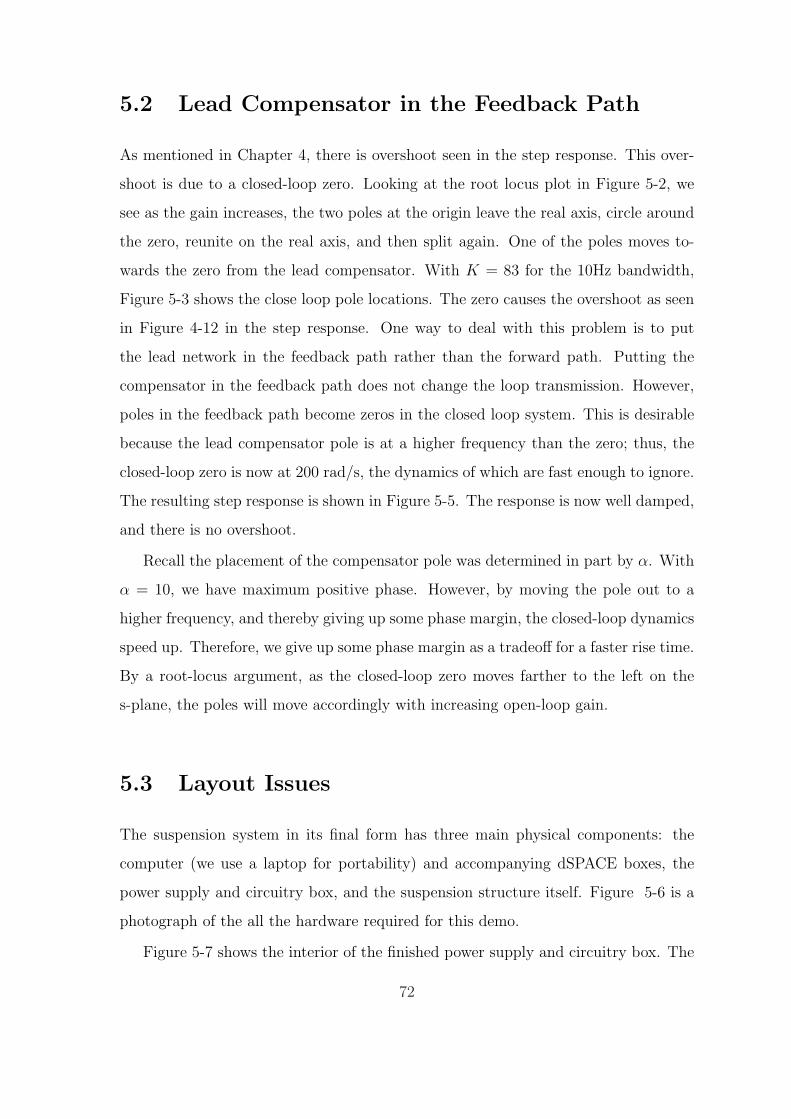
5-3 Pole-zero plot with lead compensator in the forward path. There is a

low frequency zero that effects the dynamics causing an overshoot in

the step response. . . . . . . . . . . . . . . . . . . . . . . . . . . . . . 73

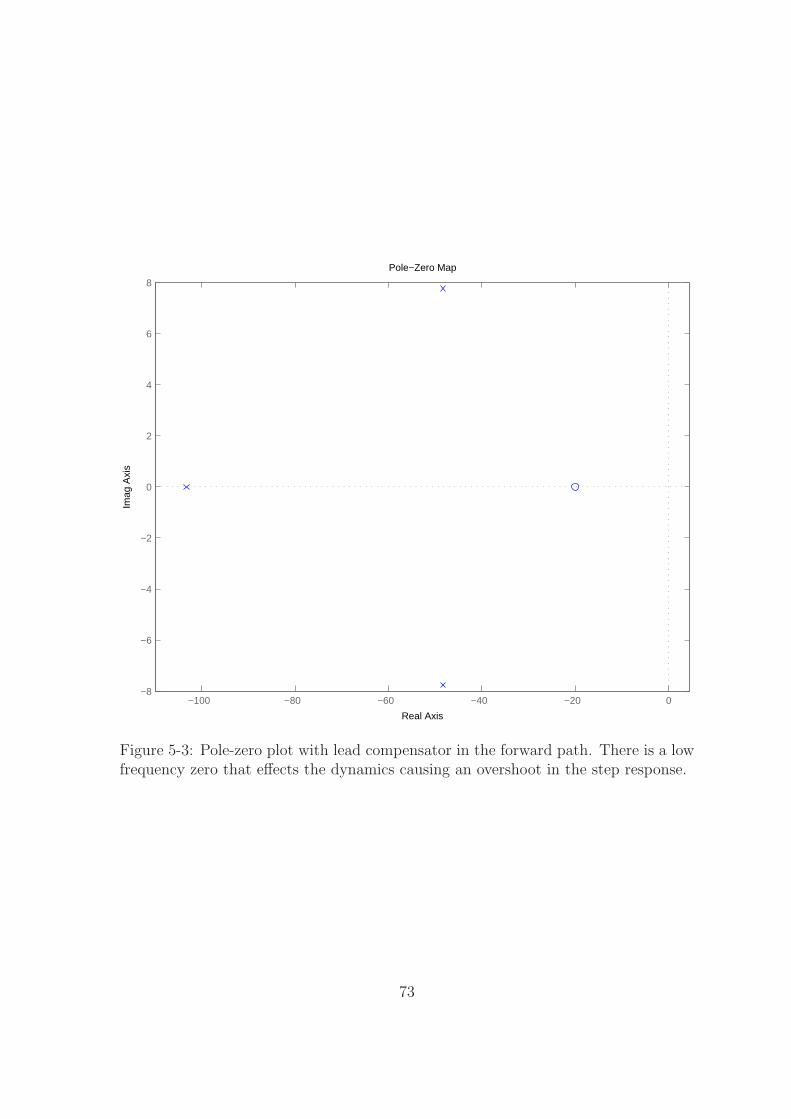
5-4 Pole-zero plot with lead compensator in the feedback path. Placing

the compensator in the feedback path moves the zero to −200 rad/s,

the location of the open loop compensator pole. With the zero at this

frequency, the dynamics are dominated by the low frequency poles. . 74

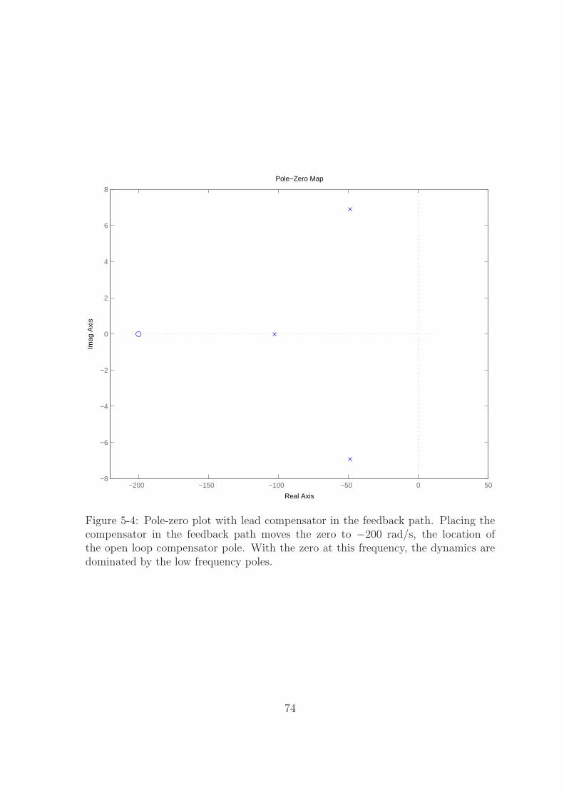
5-5 Step response of closed loop system with compensator in the feedback

path. The step response with the compensator in the forward path is

overlayed for comparison. The rise time is faster with the compensator

in the forward path but has overshoot. Settling time is about the same

for both. . . . . . . . . . . . . . . . . . . . . . . . . . . . . . . . . . . 75

5-6 Hardware for maglev demo. . . . . . . . . . . . . . . . . . . . . . . . 76

5-7 Interior of power supply and circuitry box. . . . . . . . . . . . . . . . 77

5-8 Separation of control and power circuitry. . . . . . . . . . . . . . . . . 78

5-9 Photograph of ball in suspension. . . . . . . . . . . . . . . . . . . . . 79

5-10 Photograph of ball in suspension. . . . . . . . . . . . . . . . . . . . . 80

5-11 Experimental loop transmission designed for 10 Hz bandwidth. Actual

crossover is at about 8 Hz. The DSA tool used to generate this plot

actually plots the negative loop transmission, which explains the phase

offset by 180. . . . . . . . . . . . . . . . . . . . . . . . . . . . . . . . 81

11

5-12 Experimental plant transfer function. The circles with an interpolated

line represent data points, and the single solid line is the theoretical

transfer function. The DSA tool used to generate the plot actually

plots the negative of the plant transfer function, which is why the

phase is offset by 180. . . . . . . . . . . . . . . . . . . . . . . . . . . 82

5-13 Theoretical step responses for 10, 30, and 100 Hz bandwidth designs. 84

5-14 Experimental step responses to a 0.01 N disturbance force at a 10 mm

air gap. The higher bandwidth 30 Hz crossover signal shows better

disturbance rejection. . . . . . . . . . . . . . . . . . . . . . . . . . . . 85

5-15 Position responses (voltage measurement from position sensor) to a

1 mm step at air gaps 18 mm, 15 mm, 11 mm, and 7 mm. . . . . . . 86

5-16 Coil current, as measured by the sense resistor, with a 1 mm step input

at air gaps 18 mm, 15 mm, 11 mm, and 7 mm. . . . . . . . . . . . . . 87

5-17 Photograph of ball glued to column in suspension. . . . . . . . . . . . 88

B-1 Design layout of power supply and circuitry box. Drawing courtesy of

Danny Hilton. . . . . . . . . . . . . . . . . . . . . . . . . . . . . . . . 94

C-1 Simulink model for the magnetic suspension system. . . . . . . . . . . 96

C-2 Simulink model for determining loop transmission frequency analysis. 97

12

List of Tables

5.1 Parameters for designing a controller at different bandwidths at 10Hz,

30Hz, and 100Hz. . . . . . . . . . . . . . . . . . . . . . . . . . . . . . 83

13

14

Chapter 1

Introduction

1.1 Background

This thesis presents the development of a single-axis magnetic suspension system for

use as a classroom demonstration illustrating nonlinear control. It is based on a

design originally developed by Professor David Trumper with his students at UNC

Charlotte as documented in [10] and [11]. What at first glance appears to be a simple

classroom demo, shown in Figure 1-1, actually involves many subtle complexities.

Developing a working prototype requires command of a broad range of control tech-

niques from modeling and analysis to design. Much research on control techniques

has been tested on ball suspension systems. Namerikawa et al. evaluate the effec-

tiveness of a generalized H∞ control attenuating initial state uncertainties using a

magnetic suspension system much like the one presented in this thesis [6]. Trumper

et al. compared the performance of a nonlinear and linear controller in [10]. A good

reference on magnetic suspension control techniques can be found in [9, chap. 3]. The

techniques presented extend to larger systems used in robotics, aircraft, disk drives,

and much more. Maglev trains and magnetic bearings are two of the most important

related applications.

Maglev trains have received much attention in recent years. The first commercial

maglev train made its appearance in China in December 2000. Both Japan and

Germany are developing technologies that are in the testing stages. Much faster than

15

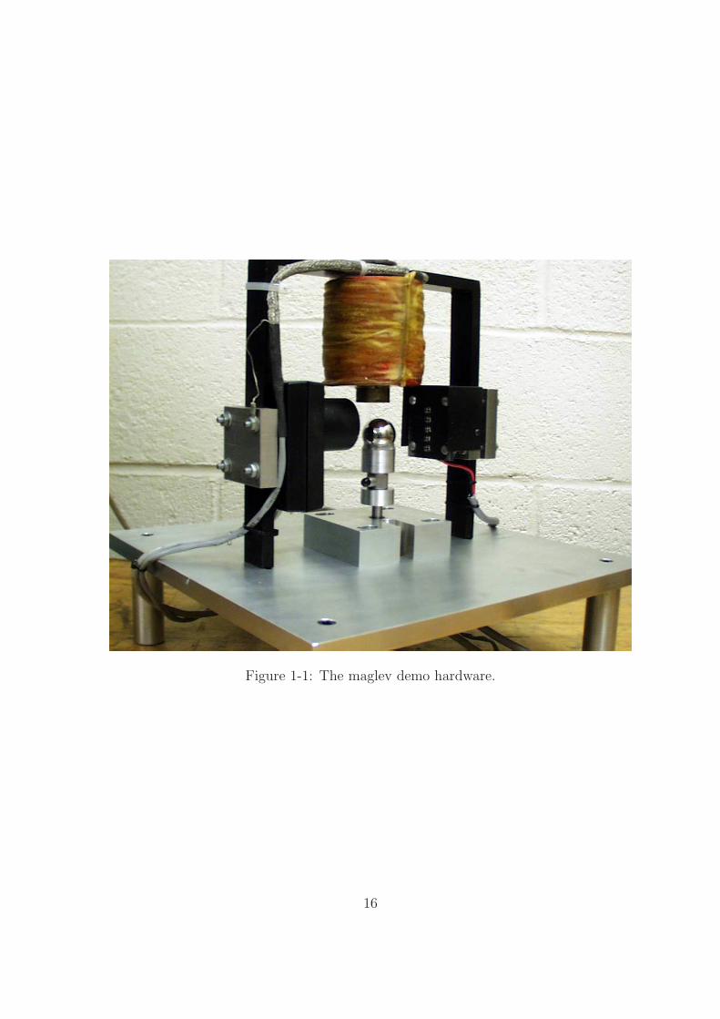
Figure 1-1: The maglev demo hardware.

16

conventional trains, maglev trains could offer an alternative to air travel. The trains

float over guide rails virtually eliminating friction, which allows them to reach speeds

of 350 mph or greater without the limitations of wheels. Such advantages could allow

this technology to revolutionize transportation. This area of research has long been

around but only recently have the costs become comparable to other technologies

such that it is no longer cost prohibitive.

Magnetic bearings have a number of advantages over conventional roller or fluid

bearings. High circumferential speeds at high loads make them ideal for use in ro-

tating machinery. Electromagnets positioned about a magnetic rotor support the

rotating shaft, thereby eliminating contact, wear, and the need for lubricants. The

lack of friction means very little loss and virtually unlimited life expectancy. These

factors permit operation in extreme environments such as high temperatures, low tem-

peratures, and vacuum. They are used in high vacuum pumps, milling and grinding

spindles, gyroscopes for space, and much more.

This thesis project demonstrates key issues by focusing on a single degree of free-

dom magnetic suspension system. It illustrates the issues associated with nonlinearity,

instability, and robustness of design. Tradeoffs exist and we need to understand which

are the important factors to be designing for, and where there is room for error. Some

performance measures we will discuss are disturbance rejection, overshoot, damping,

robustness to modeling error and unknown plant characteristics, and of course overall

stability. Any study of control systems should start with these fundamentals. Stu-

dents can learn a great deal from a relatively simple example, and such research forms

a good basis for further work in mechatronics and controls.

1.2 Overview

The levitation system consists of a position sensor, actuator, and controller. Figure 1-

2 shows a conceptual schematic of this system, and Figure 1-3 is a photograph of the

actual hardware. The actuator provides the force necessary to counteract gravity and

to stabilize the equilibrium. It is an electromagnet whose field strength depends on

17

Light

Source

Actuator

Light

DetectorController

Figure 1-2: System schematic consisting of actuator, position sensor, and controller.

the amount of current flowing in the coil. We can thus control the magnetic force

by adjusting this current. The actuator exerts force by pulling on and releasing the

ball, giving us active control over the vertical axis. The equilibrium is only passively

stabilized in the lateral directions via the field gradient. A suspension system also

requires a mechanism for sensing the position of the object, a ball in this case. Here,

we use an optical approach with a light source and corresponding sensor. As the ball

moves up and down, the amount of light detected changes accordingly. The controller

looks at the position of the ball and compares it to the reference input position,

adjusting the force as needed. The relationship between force, current, and air gap is

nonlinear. We use a micrometer fixture to measure this relationship as shown in the

picture of Figure 1-4 and the layout of Figure 1-5. Traditionally, these equations are

linearized about an operating point. Instead, we use feedback linearization, which

overcomes the operating point dependency and allows the suspension to work over a

wide range of air gaps. This thesis details the design and implementation of the the

18

Figure 1-3: Photograph of physical structure. Controller not shown.

position sensor, actuator, controller, and associated interface electronics.

Aside from feedback linearization, there are other nonlinear control techniques

worth mentioning but are beyond the scope of this paper. Adaptive gain scheduling

is one such technique. Essentially, the system of interest is linearized about several

operating points and a separate controller is designed for each. Then, a gain sched-

uler is designed to interpolate over the controllers. Kadmiry et al. use a fuzzy gain

scheduling approach to helicopter control, stabilizing attitude angles (pitch, roll, yaw)

over a large range [3]. Fuzzy gain scheduling falls in a large class of adaptive con-

trollers where unpredictable environments and dynamics that are multi-variable and

sometimes unknown require an adaptive solution. There is much interest in this area

of controls and literature is abundant. Krupadanam et al. [4] and Corban et al. [1]

offer alternative approaches to adaptive control.

19

Ball

Platform

Micrometer

Load

Cell

Figure 1-4: Drawing of the micrometer fixture.

Figure 1-5: Photograph of the micrometer fixture.

20

1.3 Organization

In Chapter 2, we develop a method for creating a model, first measuring the force,

current, and air gap relationship for this structure. We base our model on theory and

then adjust it to fit experimental data. From there, Chapter 3 outlines the circuits

used in this system. They consist of the linear amplifier, light source, and transresis-

tance amplifier. Chapter 4 formalizes some nonlinear compensation techniques and

details the controller used for this project. Chapter 5 summarizes the results and an-

alyzes some performance measures. Finally, conclusions and suggestions for further

work are discussed in Chapter 6.

21

22

Chapter 2

Circuit Implementation

2.1 Introduction

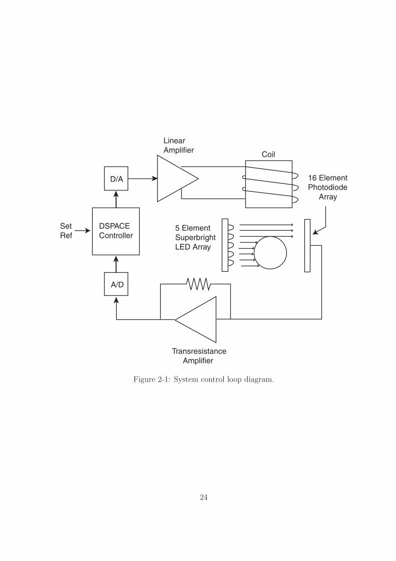
The magnetic suspension system is depicted schematically in Figure 2-1. It consists of

a position sensor, linear amplifier, controller, and actuator coil. The position sensor

uses an array of light emitting diodes as the light source and a photodiode array to

detect the light. A steel ball is suspended between the light source and detector. The

photodiode array produces a current proportional to the amount of light detected,

which in turn depends upon the position of the steel ball. The transresistance ampli-

fier converts the photodiode current into a voltage representative of position, which

the computer processes. Completing the loop, the linear amplifier takes a voltage

control signal from the computer and produces a proportional current of 0 − 2 A

to drive the coil. There are 2200 turns in the coil, wrapped on a 1” steel core. A

photograph of the actuator is shown in Figure 2-2. The computer consists of a PC,

dSPACE board, and associated software to implement the controller (see Appendix

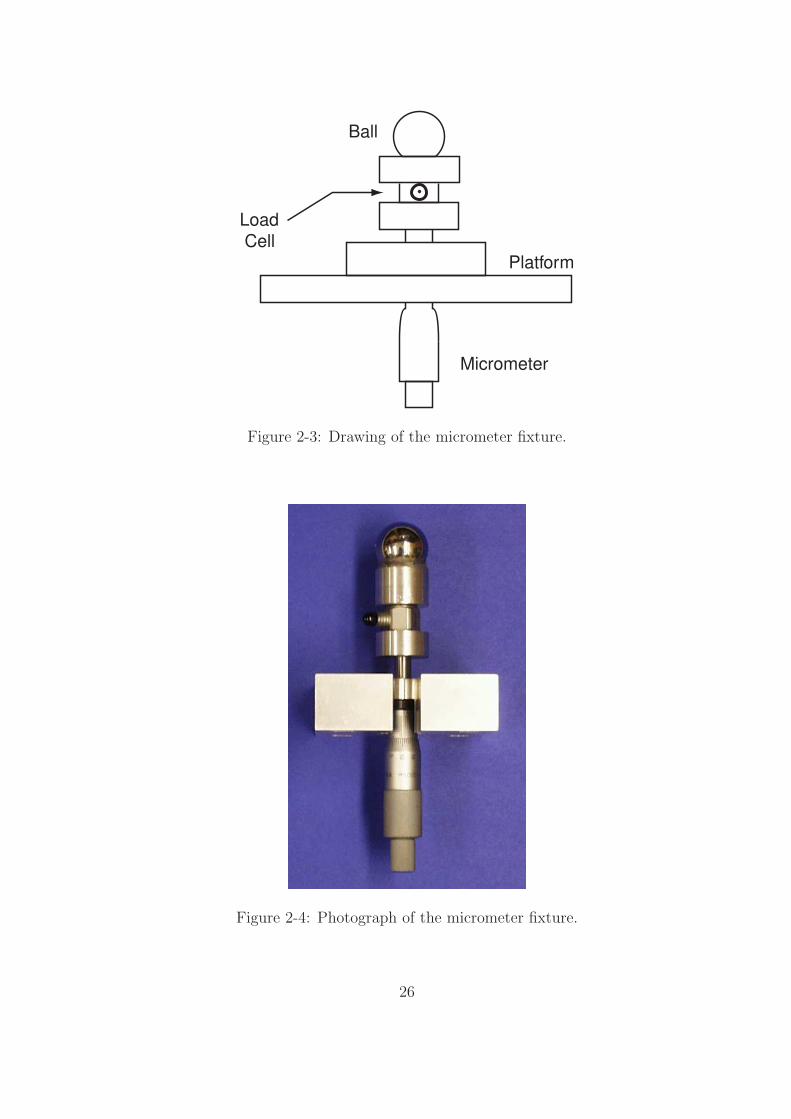
E for vendor details). The force measurement device is a micrometer attached to a

load cell with a steel ball glued onto the top, depicted in Figure 2-3. A photograph

of the micrometer is shown in Figure 2-4. We use the micrometer fixture for both

position sensor calibration and force-current relationship measurements. Instead of

implementing directly on a PC as was done in an earlier versions, this version uses

the dSPACE board in conjunction with a PC running Matlab and Simulink software.

23

DSPACE

Controller

Linear

Amplifier

D/A

A/D

Transresistance

Amplifier

5 Element

Superbright

LED Array

Coil

16 Element

Photodiode

Array

Set

Ref

Figure 2-1: System control loop diagram.

24

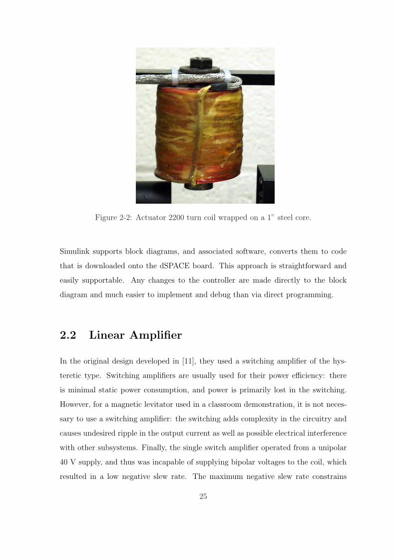
Figure 2-2: Actuator 2200 turn coil wrapped on a 1” steel core.

Simulink supports block diagrams, and associated software, converts them to code

that is downloaded onto the dSPACE board. This approach is straightforward and

easily supportable. Any changes to the controller are made directly to the block

diagram and much easier to implement and debug than via direct programming.

2.2 Linear Amplifier

In the original design developed in [11], they used a switching amplifier of the hys-

teretic type. Switching amplifiers are usually used for their power efficiency: there

is minimal static power consumption, and power is primarily lost in the switching.

However, for a magnetic levitator used in a classroom demonstration, it is not neces-

sary to use a switching amplifier: the switching adds complexity in the circuitry and

causes undesired ripple in the output current as well as possible electrical interference

with other subsystems. Finally, the single switch amplifier operated from a unipolar

40 V supply, and thus was incapable of supplying bipolar voltages to the coil, which

resulted in a low negative slew rate. The maximum negative slew rate constrains

25

Ball

Platform

Micrometer

Load

Cell

Figure 2-3: Drawing of the micrometer fixture.

Figure 2-4: Photograph of the micrometer fixture.

26

the system particularly in the case where the steel ball is drawn close to the magnet.

Only a small amount of current is needed near the pole face and therefore the current

must be rapidly decreased or the ball will overshoot, leading to issues of instability

in the loop. For good large-signal stability, we need bipolar voltage control, although

the coil current is unipolar. Here, we will be using a linear amplifier to address these

issues. This amplifier is based on a design developed by Prof. Trumper, and modified

by Xiadong Lu, a Doctoral student in Prof. Trumper’s lab.

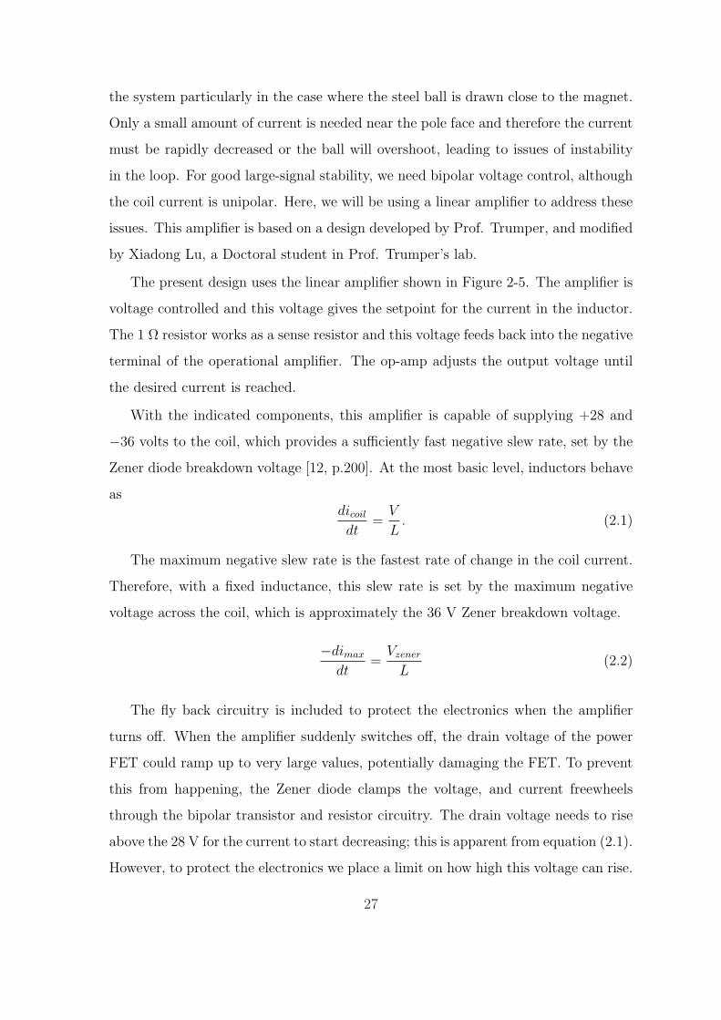
The present design uses the linear amplifier shown in Figure 2-5. The amplifier is

voltage controlled and this voltage gives the setpoint for the current in the inductor.

The 1 Ω resistor works as a sense resistor and this voltage feeds back into the negative

terminal of the operational amplifier. The op-amp adjusts the output voltage until

the desired current is reached.

With the indicated components, this amplifier is capable of supplying +28 and

−36 volts to the coil, which provides a sufficiently fast negative slew rate, set by the

Zener diode breakdown voltage [12, p.200]. At the most basic level, inductors behave

asdicoil

dt=

V

L. (2.1)

The maximum negative slew rate is the fastest rate of change in the coil current.

Therefore, with a fixed inductance, this slew rate is set by the maximum negative

voltage across the coil, which is approximately the 36 V Zener breakdown voltage.

−dimax

dt=

Vzener

L(2.2)

The fly back circuitry is included to protect the electronics when the amplifier

turns off. When the amplifier suddenly switches off, the drain voltage of the power

FET could ramp up to very large values, potentially damaging the FET. To prevent

this from happening, the Zener diode clamps the voltage, and current freewheels

through the bipolar transistor and resistor circuitry. The drain voltage needs to rise

above the 28 V for the current to start decreasing; this is apparent from equation (2.1).

However, to protect the electronics we place a limit on how high this voltage can rise.

27

28V

1k

36 V

Vin

1

R2

R1

Rs

C

82k

16k

0.01 F

pseudo-zener

coil

IRFP260N

TIP41C

OP-27

1N3070

0.1 F

0.1 F

Figure 2-5: Linear amplifier circuit.

28

Once the drain voltage reaches 28 V + 36 V = 64 V, the zener diode breaks down

and starts to conduct current in the reverse direction. Once this happens, the zener

current turns on the power transistor, which then conducts the flyback current. The

diode connected to the emitter and supply acts to prevent current flow through the

fly back circuit during normal operation where the current should flow through the

inductor path to ground. Otherwise, the power transistor base-emitter junction would

break down; the reverse breakdown voltage at that junction is only about 6 V. The

Zener voltage is chosen to be 28 V or higher, to avoid limiting of the +28/-36 V swing

across the coil as previously mentioned.

Typically in a basic fly-back circuit, a diode is simply shunted across the inductor

but this allows only 0.6 V drop. However, with the pseudo-Zener diode, we can have a

maximum of +28/-36 V across the coil during stages of increasing/decreasing current.

Thus, the performance improves on the negative slew rate over the switching amplifier

design.

However, equation (2.1) and (2.2) do not take into account the coil resistance.

We measured the coil resistance to be about 30 Ω. At best, the maximum positive

voltage across the inductor is given by

VL = Vsupply − iRL. (2.3)

The OP-27 used in this design has a gain on the order of 106 (1.8 million) at low

frequencies and a unity gain bandwidth of 10 MHz. This is far too much bandwidth

for the application at hand; forcing crossover at 1 kHz, which sufficiently exceeds

the closed loop bandwidth, stabilizes the loop. We also get better noise rejection by

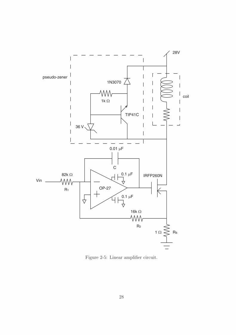
forcing a crossover at 1 kHz. The closed loop is modeled in Figure 2-6 where the gate

to source gain is approximately 1, (i.e. the FET acts as a follower). We want the

magnitude of the loop transmission to equal 1 at 1kHz, and the loop transmission is

given by

L.T. =−1

R2Cs. (2.4)

29

1

1

1

R

1

Cs

2

1

R

1i

2i

gateV

senseVref

V

Figure 2-6: Block diagram for amplifier circuit.

We first choose a reasonable value for C - 0.01 µF. This then requires R2 = 16 kΩ.

The digital to analog converter in dSPACE outputs voltage in the range of ±10 V.

Ideally, for the highest resolution the full range would be used to map to the current

command. For simplicity, we only map the command to the positive side from 0-

10 V. We found the maximum current needed is 2 A (more on current requirements

in Chapter 4). Therefore, 0− 10 V maps to 0− 2 A or

Vsense

Vref

=1

5. (2.5)

The resistor R1 is thus constrained by the gain requirement at DC

Vsense

Vref

=R2

R1(R2Cs + 1)⇒ D.C.gain =

R2

R1

, (2.6)

which gives R1 = 5R2 = 80 kΩ. However, we encountered problems with stability

using a gain of 1/5 in the amplifier, the reasons for which have yet to be worked out.

The system appears to work fine with a unity gain in the amplifier so that is how it

is currently implemented.

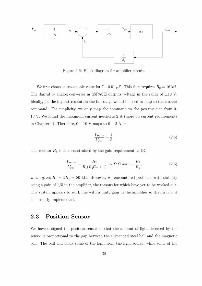
2.3 Position Sensor

We have designed the position sensor so that the amount of light detected by the

sensor is proportional to the gap between the suspended steel ball and the magnetic

coil. The ball will block some of the light from the light source, while some of the

30

light will pass through. Ideally, when the gap is zero, no light passes into the detector

because the ball has completely blocked the light coming from the source. On the

receiving end, there is a red filter in front of the sensor to attenuate light coming from

other sources, such as ambient lighting.

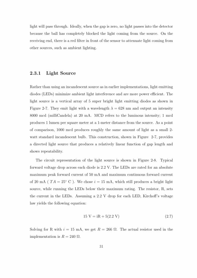
2.3.1 Light Source

Rather than using an incandescent source as in earlier implementations, light emitting

diodes (LEDs) minimize ambient light interference and are more power efficient. The

light source is a vertical array of 5 super bright light emitting diodes as shown in

Figure 2-7. They emit light with a wavelength λ = 628 nm and output an intensity

8000 mcd (milliCandela) at 20 mA. MCD refers to the luminous intensity; 1 mcd

produces 1 lumen per square meter at a 1-meter distance from the source. As a point

of comparison, 1000 mcd produces roughly the same amount of light as a small 2-

watt standard incandescent bulb. This construction, shown in Figure 2-7, provides

a directed light source that produces a relatively linear function of gap length and

shows repeatability.

The circuit representation of the light source is shown in Figure 2-8. Typical

forward voltage drop across each diode is 2.2 V. The LEDs are rated for an absolute

maximum peak forward current of 50 mA and maximum continuous forward current

of 20 mA ( TA = 25 C ). We chose i = 15 mA, which still produces a bright light

source, while running the LEDs below their maximum rating. The resistor, R, sets

the current in the LEDs. Assuming a 2.2 V drop for each LED, Kirchoff’s voltage

law yields the following equation:

15 V = iR + 5(2.2 V) (2.7)

Solving for R with i = 15 mA, we get R = 266 Ω. The actual resistor used in the

implementation is R = 240 Ω.

31

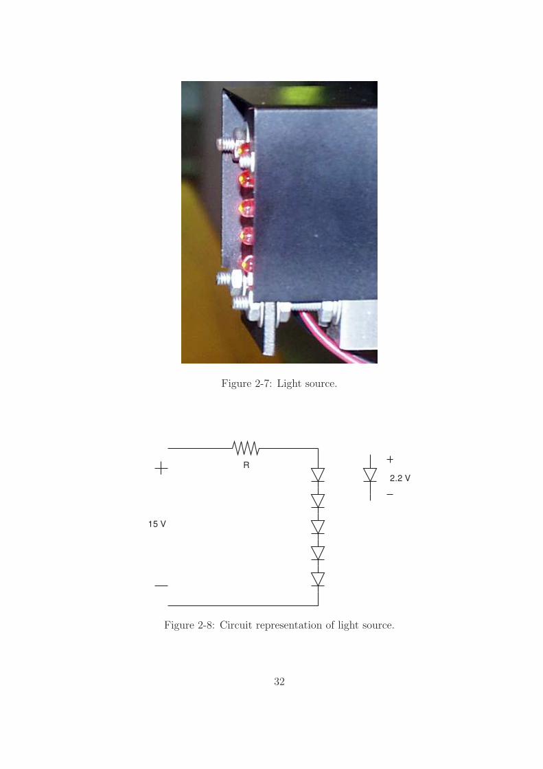
Figure 2-7: Light source.

R

15 V

2.2 V

Figure 2-8: Circuit representation of light source.

32

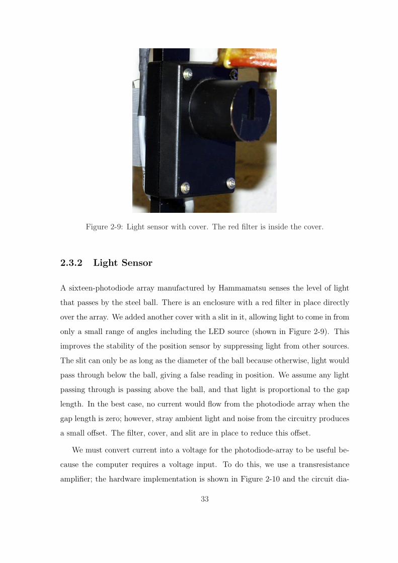
Figure 2-9: Light sensor with cover. The red filter is inside the cover.

2.3.2 Light Sensor

A sixteen-photodiode array manufactured by Hammamatsu senses the level of light

that passes by the steel ball. There is an enclosure with a red filter in place directly

over the array. We added another cover with a slit in it, allowing light to come in from

only a small range of angles including the LED source (shown in Figure 2-9). This

improves the stability of the position sensor by suppressing light from other sources.

The slit can only be as long as the diameter of the ball because otherwise, light would

pass through below the ball, giving a false reading in position. We assume any light

passing through is passing above the ball, and that light is proportional to the gap

length. In the best case, no current would flow from the photodiode array when the

gap length is zero; however, stray ambient light and noise from the circuitry produces

a small offset. The filter, cover, and slit are in place to reduce this offset.

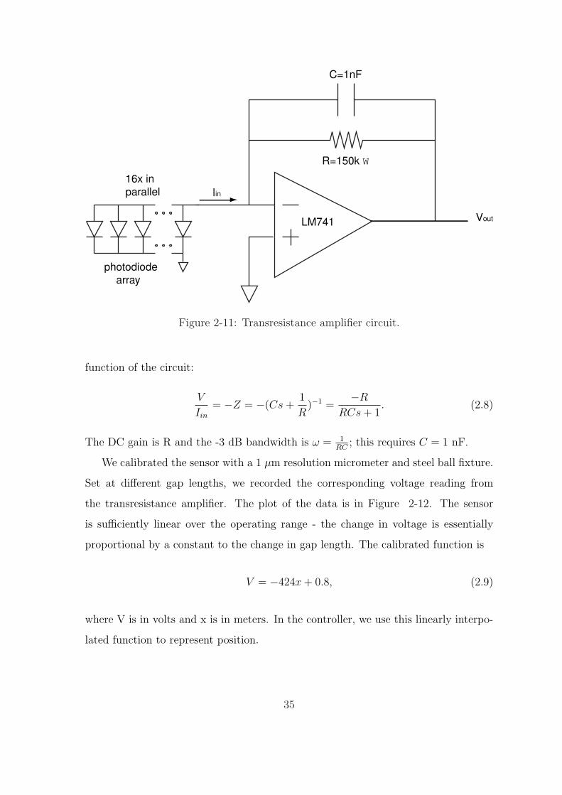
We must convert current into a voltage for the photodiode-array to be useful be-

cause the computer requires a voltage input. To do this, we use a transresistance

amplifier; the hardware implementation is shown in Figure 2-10 and the circuit dia-

33

Figure 2-10: Light sensor circuit hardware.

gram in Figure 2-11. The current is summed from all 16 photodiodes at the virtual

ground node of the transresistance amplifier. A resistor connected between the nonin-

verting terminal and output terminal of the operational amplifier acts as a transducer

to covert the current into a voltage through Ohm’s Law (V = IR).

Again, the dSPACE converter, analog to digital this time, limits the range of

meaningful input voltage, in the range of ±10 V. It is necessary to ensure the voltage

readings from the light sensor remains in these limits, but also utilizes most of the

available range. We experimentally found the maximum current reading from the

photodiode, i.e. in the case where the ball is not suspended, Imax = 6× 10−5 A . For

the full 10 V swing, this would require R = 166 kΩ. To err on the safe side, we chose

R = 150 kΩ.

A shunt capacitor C is added for low pass filtering, setting the bandwidth at

1 kHz. Solving for the impedance of the resistor/capacitor network gives the transfer

34

Iin

C=1nF

R=150k W

Vout

16x in

parallel

photodiode

array

LM741

Figure 2-11: Transresistance amplifier circuit.

function of the circuit:

V

Iin

= −Z = −(Cs +1

R)−1 =

−R

RCs + 1. (2.8)

The DC gain is R and the -3 dB bandwidth is ω = 1RC

; this requires C = 1 nF.

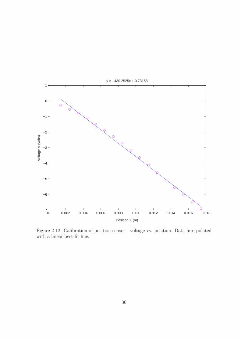
We calibrated the sensor with a 1 µm resolution micrometer and steel ball fixture.

Set at different gap lengths, we recorded the corresponding voltage reading from

the transresistance amplifier. The plot of the data is in Figure 2-12. The sensor

is sufficiently linear over the operating range - the change in voltage is essentially

proportional by a constant to the change in gap length. The calibrated function is

V = −424x + 0.8, (2.9)

where V is in volts and x is in meters. In the controller, we use this linearly interpo-

lated function to represent position.

35

0 0.002 0.004 0.006 0.008 0.01 0.012 0.014 0.016 0.018−7

−6

−5

−4

−3

−2

−1

0

1y = −430.2525x + 0.73158

Position X (m)

Vol

tage

V (

volts

)

Figure 2-12: Calibration of position sensor - voltage vs. position. Data interpolatedwith a linear best-fit line.

36

Chapter 3

Force Measurement

3.1 Introduction

For feedback linearization to be successful, it is necessary to develop an accurate model

of the system. The algebraic transformation makes this approach heavily dependent

on careful modeling of all dynamics and minimizing errors in modeling. It is one of

the drawbacks of this technique because there are situations where such modeling is

not possible. We develop an approach to modeling based on a mix of theory and

experimentally-determined results.

3.2 Theory

The physics of the setup is similar to that developed in [13, pgs.22-23, 84-86] except

it is inverted such that gravity acts to open the air gap. The key equation to take

from [13] is the force produced by the electromagnet

F = C

(i

x

)2

. (3.1)

Here, F (Newtons) is the force applied to the ball, x (m) is gap spacing between

the pole of the electromagnet and the ball, and i (Amperes) is the current through

the inductor. The gap length is increasing in the downward direction; therefore, a

37

B

H

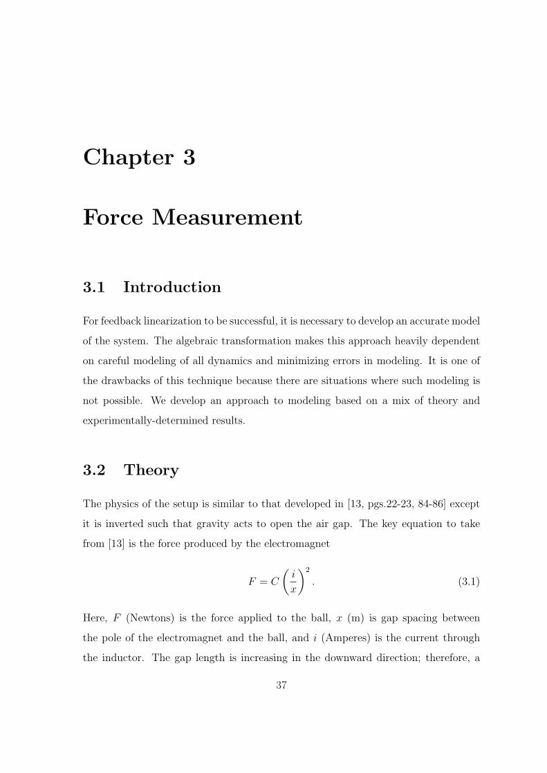
Figure 3-1: Hysteresis in B-H curve for a magnetic material.

large value of x places the ball far from the pole face. It is important to keep in

mind equation (3.1) is a simplified approximation for our system, as it ignores many

nonidealities. Later, we supplement the model with experimental data accounting for

these differences. Specifically, the equation does not account for a number of effects

including finite core reluctance, saturation of the core, magnetic hysteresis, and eddy

currents in the core. We address each of these issues in turn.

The ideal case assumes the path of magnetic flux has infinite permeability every-

where except at the variable air gap. All the flux would then be concentrated in the

air gap. Analyzing this as a magnetic circuit, the flux path would be the wire, coil

ampere turns the voltage source, air gap the resistor, and flux the current. As the air

gap closes, the resistance approaches zero. Therefore, the current goes to infinity, or

analogously, the flux goes to infinity. In reality, just as there is parasitic resistance in

a real wire, there is a finite reluctance in our magnetic path. The force on the ball

is not infinite with zero gap space as (3.1) would suggest. We must account for this

non-ideality, and we do so by adding a constant factor, x0, to the gap length in the

38

denominator. This results in a finite value as x approaches zero. We later determine

this value experimentally.

Three additional characteristics of magnetic materials require attention: hystere-

sis, saturation, and finite conductivity. There is hysteresis in ferromagnetic materials

that tend to stay magnetized even after the applied field has been turned off or re-

versed in direction. This produces a curve as shown in Figure 3-1. Depending on

whether the current is increasing or decreasing, there is thus a different force value

for a given current level. Therefore, the magnetic flux is dependent on both current

and the prior history of magnetization. This can be a problem for systems where

very precise values of magnetic flux are needed but is not necessarily troublesome in

all situations. Later, we develop a model for linearization in our controller based on

these force measurements; therefore, an acceptable representation of magnetic flux

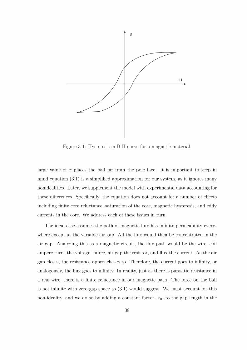
values must be developed. Fortunately, for this magnetic suspension the issue is re-

solved to an acceptable degree simply by taking the arithmetic mean of the hysteretic

curve. We split the curves into 2 and average the values point by point. The result

is a monotonic, averaged function relating the force and current. In Figure 3-2 this

function is the dashed line. Heuristically, this turned out to be a sufficient solution.

The force is still smoothly controllable, despite the hysteresis, unlike Coulomb fric-

tion where there are sudden changes in value. Choosing a magnetically softer core

material would also reduce this problem.

Saturation occurs in all iron-core electromagnets. The flux density levels off for

increasing amounts of field intensity. Essentially, when a small amount of force is

applied, the domains in the magnetic material easily align to increase the flux density.

However, as more flux is crammed into the cross-sectional area, there are fewer and

fewer domains available. At this point, it will take more force to produce the same

amount of flux density. This saturation accounts for a large part for the terms we

will add in the transformation equation from force to current. For our electromagnet,

due to saturation, equation (3.1) is only a reasonable fit for currents i ≤ 0.4 A.

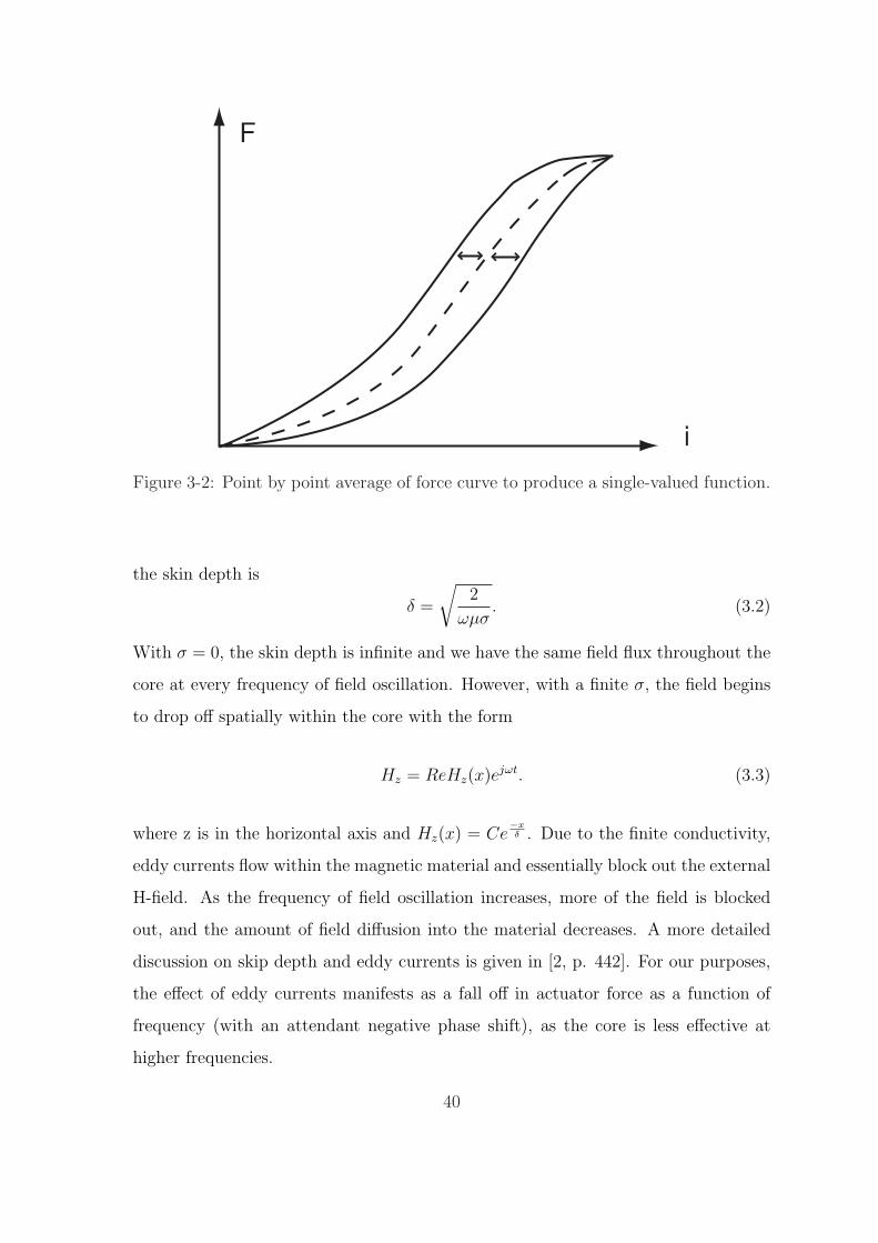
Finally, we address the effects of eddy currents in the core. The solid core has a

conductivity σ and permeability µ. For the frequency of magnetic field oscillation ω,

39

i

F

Figure 3-2: Point by point average of force curve to produce a single-valued function.

the skin depth is

δ =

√2

ωµσ. (3.2)

With σ = 0, the skin depth is infinite and we have the same field flux throughout the

core at every frequency of field oscillation. However, with a finite σ, the field begins

to drop off spatially within the core with the form

Hz = ReHz(x)ejωt. (3.3)

where z is in the horizontal axis and Hz(x) = Ce−xδ . Due to the finite conductivity,

eddy currents flow within the magnetic material and essentially block out the external

H-field. As the frequency of field oscillation increases, more of the field is blocked

out, and the amount of field diffusion into the material decreases. A more detailed

discussion on skip depth and eddy currents is given in [2, p. 442]. For our purposes,

the effect of eddy currents manifests as a fall off in actuator force as a function of

frequency (with an attendant negative phase shift), as the core is less effective at

higher frequencies.

40

3.3 Methodology

We proceed by developing experiments to determine C and x0 in the model:

F = C

(i

x + x0

)2

+ additional terms. (3.4)

The constant C is dependent on material properties and physical structure. Finally,

we included additional terms to account for saturation and approximations in geom-

etry to fit the experimental data to be discussed later.

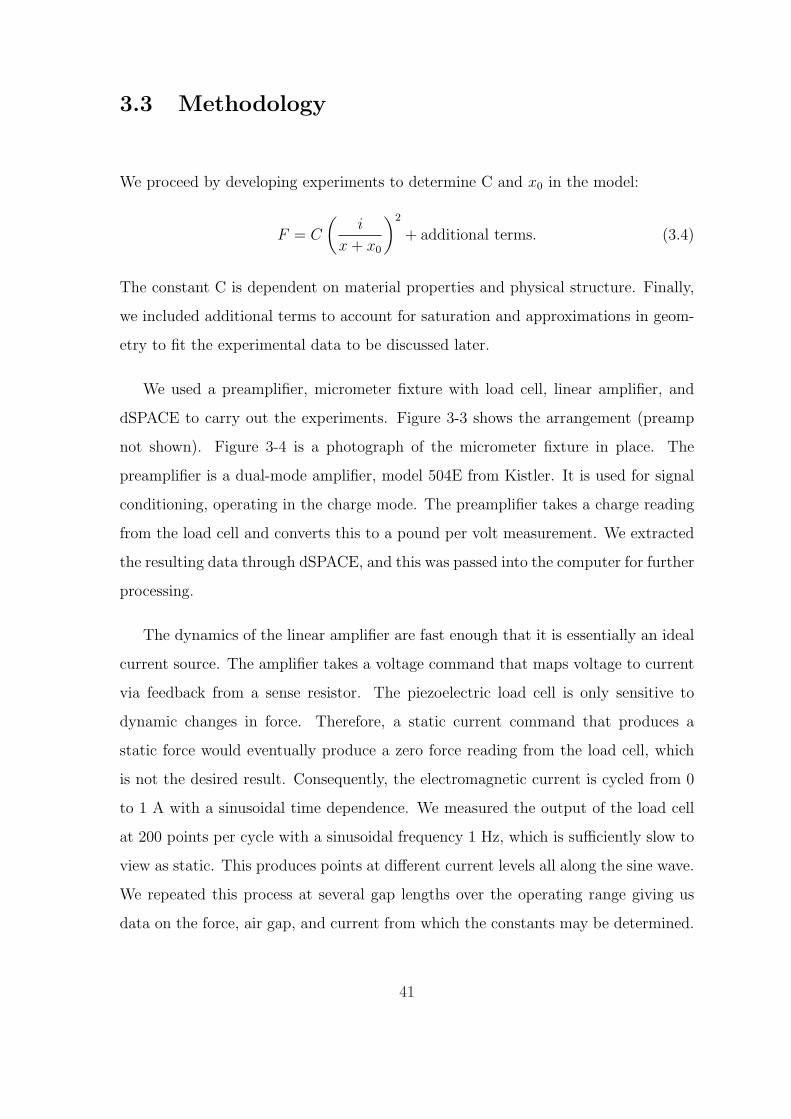
We used a preamplifier, micrometer fixture with load cell, linear amplifier, and

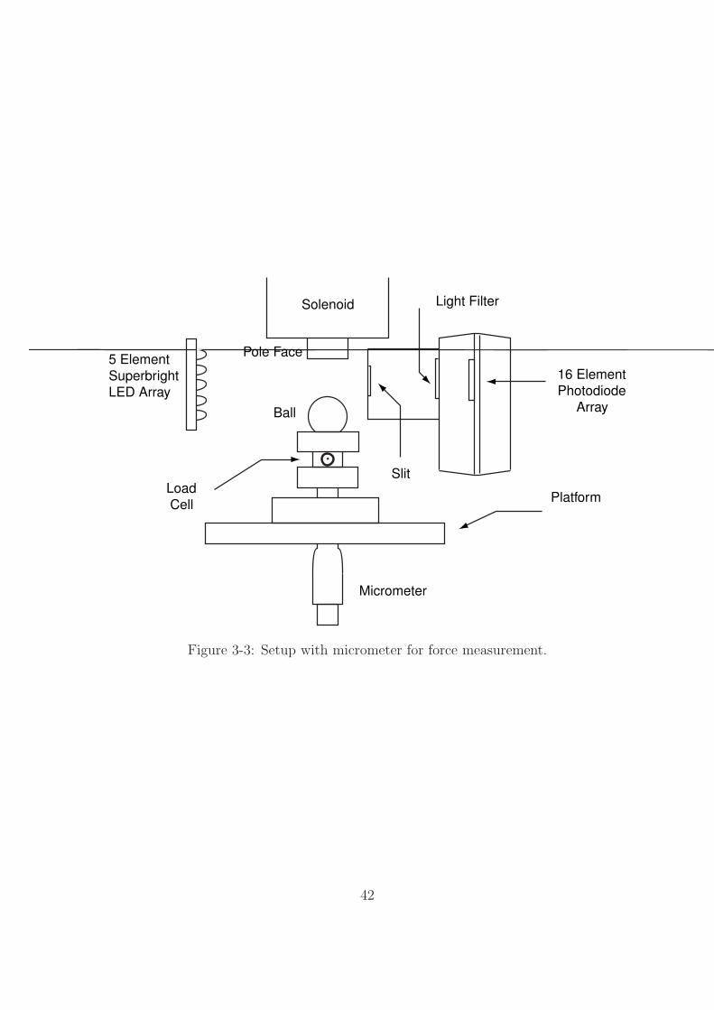
dSPACE to carry out the experiments. Figure 3-3 shows the arrangement (preamp

not shown). Figure 3-4 is a photograph of the micrometer fixture in place. The

preamplifier is a dual-mode amplifier, model 504E from Kistler. It is used for signal

conditioning, operating in the charge mode. The preamplifier takes a charge reading

from the load cell and converts this to a pound per volt measurement. We extracted

the resulting data through dSPACE, and this was passed into the computer for further

processing.

The dynamics of the linear amplifier are fast enough that it is essentially an ideal

current source. The amplifier takes a voltage command that maps voltage to current

via feedback from a sense resistor. The piezoelectric load cell is only sensitive to

dynamic changes in force. Therefore, a static current command that produces a

static force would eventually produce a zero force reading from the load cell, which

is not the desired result. Consequently, the electromagnetic current is cycled from 0

to 1 A with a sinusoidal time dependence. We measured the output of the load cell

at 200 points per cycle with a sinusoidal frequency 1 Hz, which is sufficiently slow to

view as static. This produces points at different current levels all along the sine wave.

We repeated this process at several gap lengths over the operating range giving us

data on the force, air gap, and current from which the constants may be determined.

41

5 Element

Superbright

LED Array

Pole Face

Ball

Light Filter

16 Element

Photodiode

Array

Platform

Micrometer

Load

Cell

Slit

Solenoid

Figure 3-3: Setup with micrometer for force measurement.

42

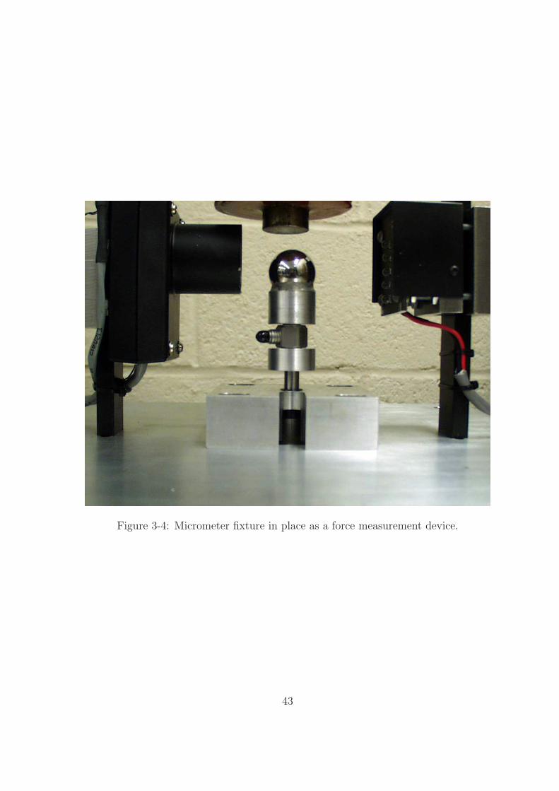
Figure 3-4: Micrometer fixture in place as a force measurement device.

43

3.4 Data Analysis

Using ControlDesk, a dSPACE software tool, we recorded measurements and saved

the data in a format readable by Matlab. The files were then imported into Matlab

for post-experimental processing. The data were in separate files associating to a

given gap length, and within each file is recorded a force vs. current relationship.

Ultimately, we would like to have a matrix with force, current, and air gap, each as

a separate column vector in a matrix.

The first step was to extract the 2 variables, force and current, and then tag each

data pair with its associated gap length. Therefore, within a file each data pair will

have the same value in the third column of the matrix.

f1 i1 x1

f2 i2 x1

f3 i3 x1

. . .

. . .

(3.5)

We create a matrix like the one above for each file. Finally, the matrices are appended

together. This makes it possible to examine the relationships of the 3 variables in

any permutation (see Appendix D for Matlab code).

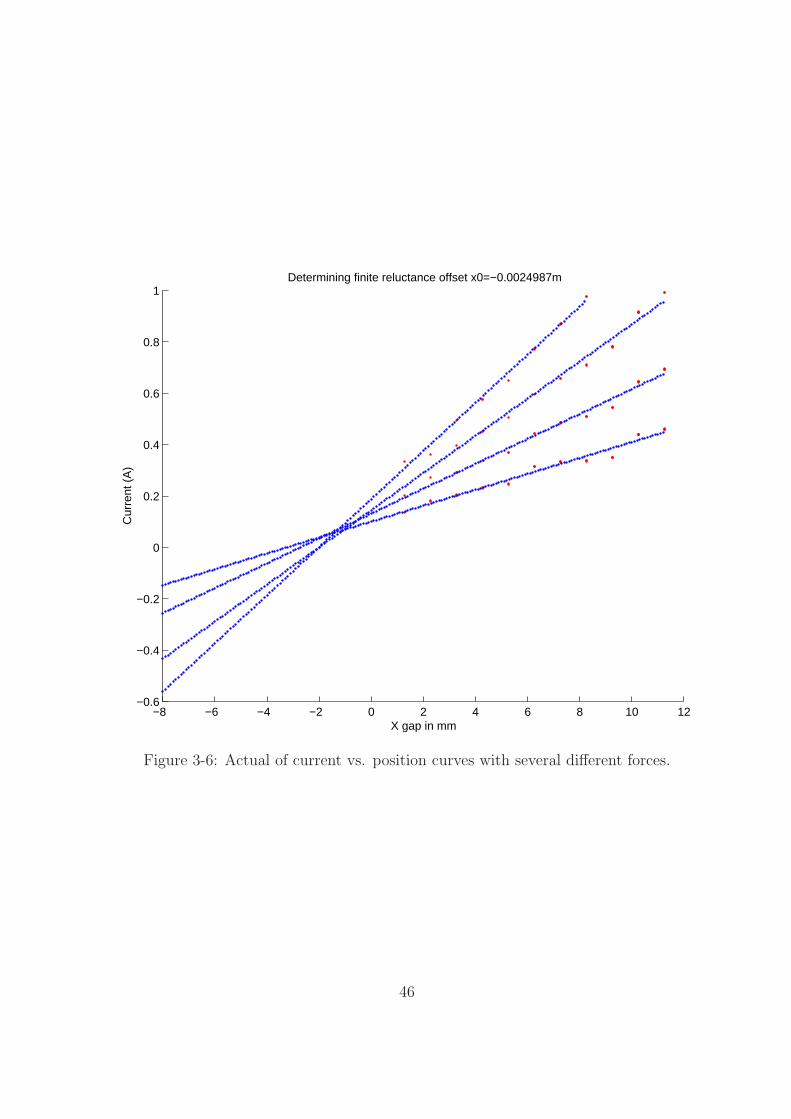
Equation (3.1) would result if the iron core had infinite permeability or zero reluc-

tance. However, the permeability is finite and that means some of the reluctance is in

the core. Due to the finite permeability, a term x0 is added to the equation (3.4). This

is determined by plotting a family of force curves with current as a function of gap

spacing (see Figure 3-5). In the ideal zero reluctance case, the curves would intersect

at x = 0. However, for the measured data they intersect at x = −0.0025 m. Solving

for the current as a function of x, we see where the curve intersects the horizontal

axis is x = −x0, or x0 = 0.0025 m, which is modeled as

i =

√F

C(x + x0). (3.6)

44

f1

f2

f3

-Xo

x

i

Figure 3-5: Predicted shape of current vs. position curves with several different forces.

The variable F changes the slope of the curve and x0 is the offset in x. At every

value of F, the curves should all intersect at x0. The experimental data is plotted in

Figure 3-6, and we see it closely matches the predicted results.

The constant C has units of Nm2

A2 and is dependent on the geometry of the setup,

and materials. Here, we determine it experimentally. Earlier work assumed this value

to be a constant. We found that the constant is more closely a linear function of x.

Including this in our transformation adds accuracy to our modeling. Plotting force

versus current, we see that for a constant force, there are current values associated

with each gap length. Solving for C gives:

C = F(x + x0)

2

i2(3.7)

A plot of C vs. x at different force values is shown in Figure 3-7. The linearly

interpolated function gives

C = −0.003x + 6.5× 10−4 (3.8)

where C is in Nm2/A2 and x in mm.

Finally, additional terms are needed in the transformation as the actual data does

not represent a square root fit throughout. The first part of the curve is roughly a

45

−8 −6 −4 −2 0 2 4 6 8 10 12−0.6

−0.4

−0.2

0

0.2

0.4

0.6

0.8

1Determining finite reluctance offset x0=−0.0024987m

X gap in mm

Cur

rent

(A

)

Figure 3-6: Actual of current vs. position curves with several different forces.

46

0.3 0.4 0.5 0.6 0.7 0.8 0.9 14.6

4.8

5

5.2

5.4

5.6

5.8

6

6.2

6.4

6.6x 10

−4 C values at f=2.8N Cave=5.2786x 10−4 NA2/m2

X gap in cm

C c

onst

ant (

NA

2 /m2 )

Figure 3-7: Plot of values of C as a function of air gap at different force values.

47

square

root

linear

squared

i

F

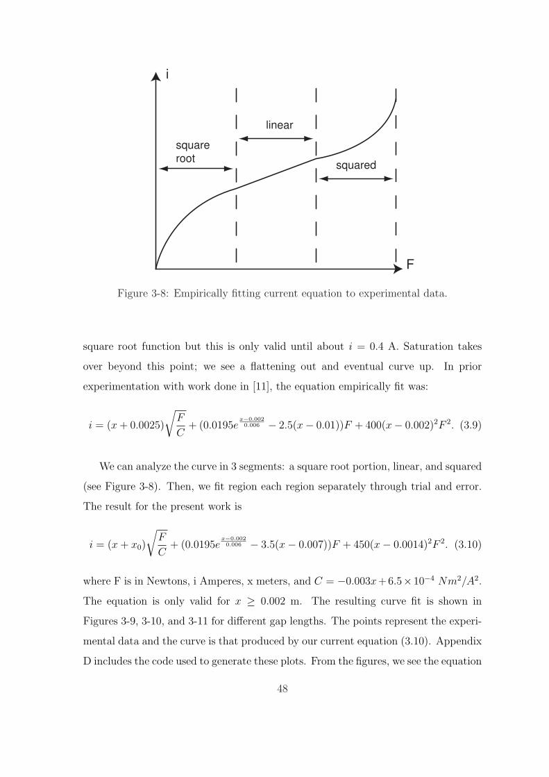
Figure 3-8: Empirically fitting current equation to experimental data.

square root function but this is only valid until about i = 0.4 A. Saturation takes

over beyond this point; we see a flattening out and eventual curve up. In prior

experimentation with work done in [11], the equation empirically fit was:

i = (x + 0.0025)

√F

C+ (0.0195e

x−0.0020.006 − 2.5(x− 0.01))F + 400(x− 0.002)2F 2. (3.9)

We can analyze the curve in 3 segments: a square root portion, linear, and squared

(see Figure 3-8). Then, we fit region each region separately through trial and error.

The result for the present work is

i = (x + x0)

√F

C+ (0.0195e

x−0.0020.006 − 3.5(x− 0.007))F + 450(x− 0.0014)2F 2. (3.10)

where F is in Newtons, i Amperes, x meters, and C = −0.003x+6.5×10−4 Nm2/A2.

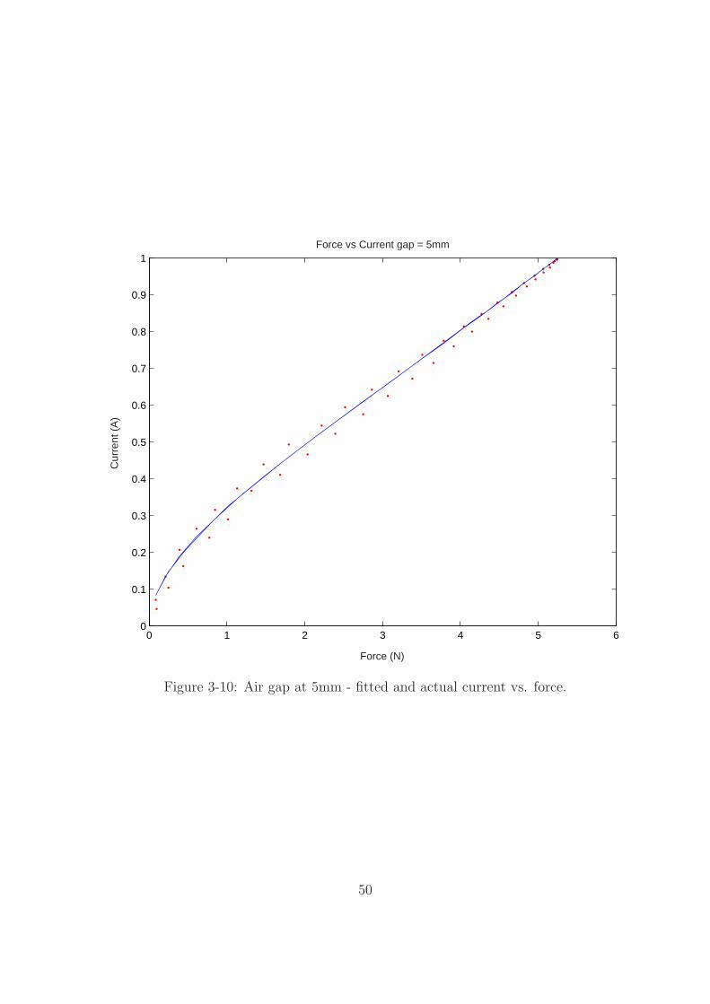
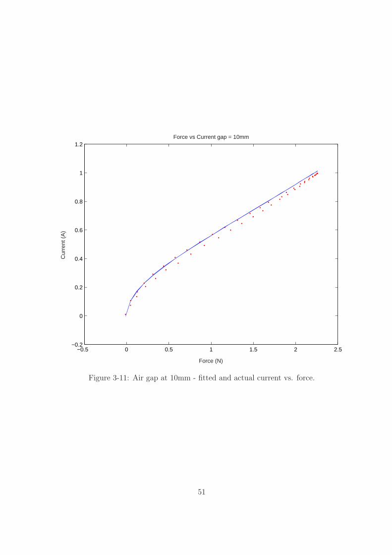
The equation is only valid for x ≥ 0.002 m. The resulting curve fit is shown in

Figures 3-9, 3-10, and 3-11 for different gap lengths. The points represent the experi-

mental data and the curve is that produced by our current equation (3.10). Appendix

D includes the code used to generate these plots. From the figures, we see the equation

48

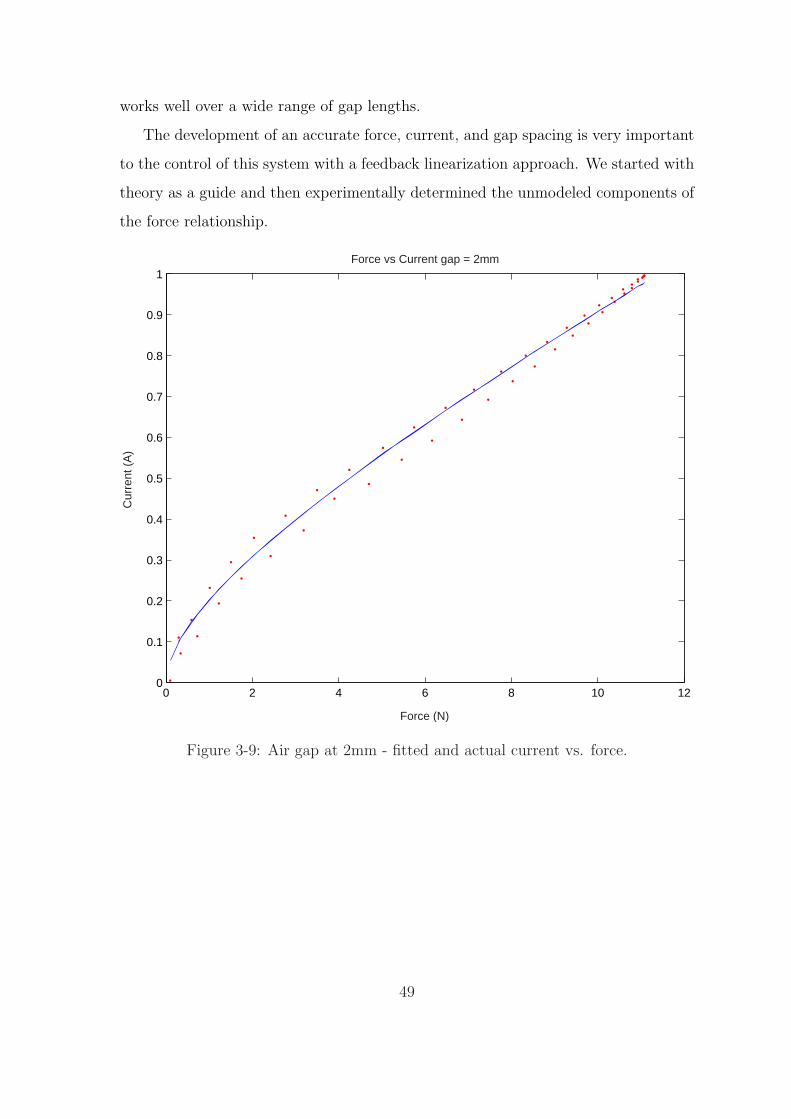
works well over a wide range of gap lengths.

The development of an accurate force, current, and gap spacing is very important

to the control of this system with a feedback linearization approach. We started with

theory as a guide and then experimentally determined the unmodeled components of

the force relationship.

0 2 4 6 8 10 120

0.1

0.2

0.3

0.4

0.5

0.6

0.7

0.8

0.9

1Force vs Current gap = 2mm

Cur

rent

(A

)

Force (N)

Figure 3-9: Air gap at 2mm - fitted and actual current vs. force.

49

0 1 2 3 4 5 60

0.1

0.2

0.3

0.4

0.5

0.6

0.7

0.8

0.9

1Force vs Current gap = 5mm

Cur

rent

(A

)

Force (N)

Figure 3-10: Air gap at 5mm - fitted and actual current vs. force.

50

−0.5 0 0.5 1 1.5 2 2.5−0.2

0

0.2

0.4

0.6

0.8

1

1.2Force vs Current gap = 10mm

Cur

rent

(A

)

Force (N)

Figure 3-11: Air gap at 10mm - fitted and actual current vs. force.

51

52

Chapter 4

Nonlinear Control Theory

4.1 Linearization

If you hold a ball up and let go, it falls because of gravity. It is necessary to cancel

this downward force with the force produced by the actuator, the electromagnet.

The suspension of a ball with an electromagnet is difficult because it is open-loop

unstable and there is a nonlinear relationship between force, current, and air gap

between the pole of the electromagnet and ball. With a fixed field strength, the

ball “feels” it more the closer it gets to the magnet. Equilibrium is reached when the

magnetic force balances the gravitational force. The instability arises because a slight

deviation from this equilibrium drives the ball further from the equilibrium point. We

traditionally solve this nonlinear controls problem by linearizing about an operating

point and then proceeding with the usual control techniques for linear systems. The

idea is to approximate the system behavior over a limited range. Here, we present

this approach as a point of comparison and to show the inherent open-loop instability

of the system. The second half of the chapter is devoted to the alternative method

via feedback linearization. The controller implemented for this project uses feedback

linearization to allow operation over a wide range of air gaps.

Using Newtonian mechanics, we write the force equations on the ball based on

53

mg

Fm x

Electromagnet

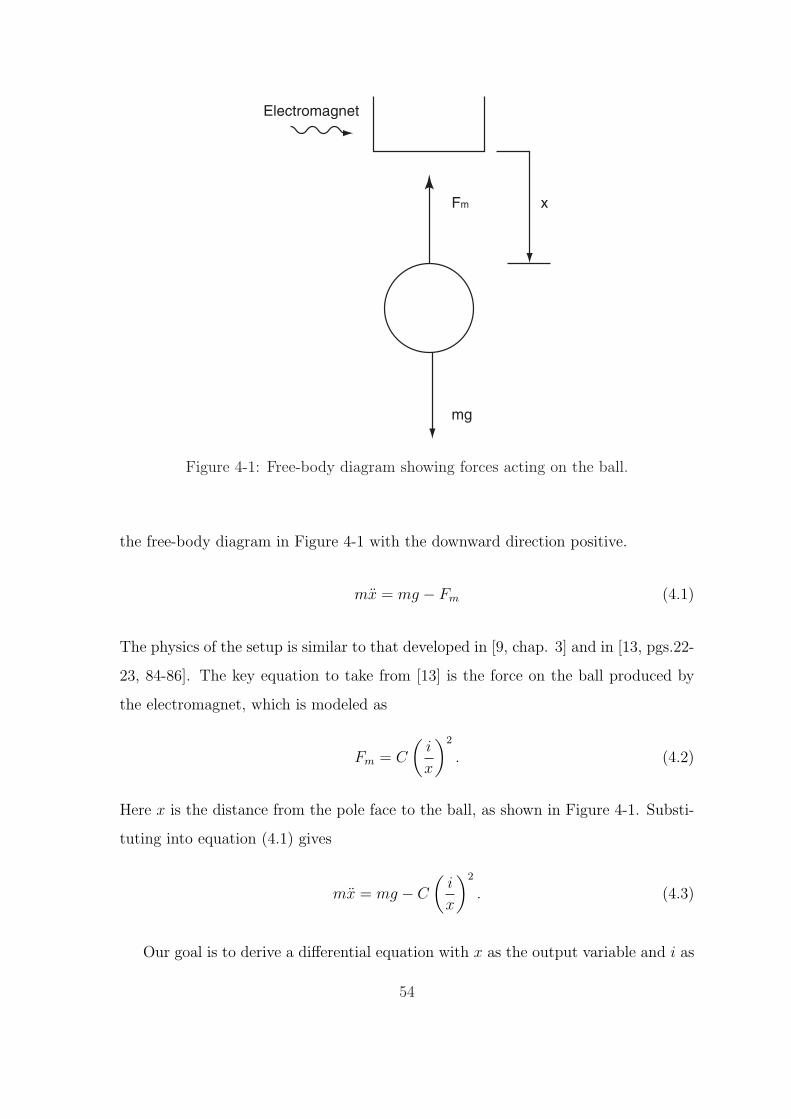
Figure 4-1: Free-body diagram showing forces acting on the ball.

the free-body diagram in Figure 4-1 with the downward direction positive.

mx = mg − Fm (4.1)

The physics of the setup is similar to that developed in [9, chap. 3] and in [13, pgs.22-

23, 84-86]. The key equation to take from [13] is the force on the ball produced by

the electromagnet, which is modeled as

Fm = C

(i

x

)2

. (4.2)

Here x is the distance from the pole face to the ball, as shown in Figure 4-1. Substi-

tuting into equation (4.1) gives

mx = mg − C

(i

x

)2

. (4.3)

Our goal is to derive a differential equation with x as the output variable and i as

54

the input variable and linearize this equation based on a tangential approximation.

Since the force is dependent on both current and air gap, we must linearize about

two variables.

i = i + i

x = x + x (4.4)

The bar ¯ notation represents the equilibrium operating point and tilde ~ represents

small deviations from this equilibrium. The linearized equation for the force is based

on a Taylor series expansion, and because this is a 1st order approximation, we drop

the higher order terms to give

Fm = C

(i

x

)2

+∂Fm

∂x|x +

∂Fm

∂i|i + higher order terms. (4.5)

Solving the partial differentials we get

∂Fm

∂x| = −2C

i2

x3x ≡ −k1x

∂Fm

∂i| = 2C

i

x2i ≡ k2i. (4.6)

The equilibrium point is where mx = 0. Therefore,

mg − C

(i

x

)2

= 0

or

mg = C

(i

x

)2

. (4.7)

Substituting (4.7) into (4.6) and then (4.6) into (4.1), we arrive at

mx = mg − C

(i

x

)2

+ k1x− k2i. (4.8)

55

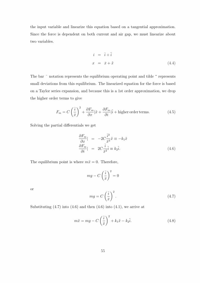
Re

Im

s2s1

Figure 4-2: Pole zero plot of linearized system.

Using (4.8) and rearranging, our final linearized equation is

mx− k1x = −k2i. (4.9)

Since k1 > 0, the poles of the system are

s1 = −√

k1

m

s2 = +

√k1

m. (4.10)

Notice there is a right half plane pole, which in the linear model represents the open-

loop instability of the system. Figure 4-2 shows the pole-zero plot in the complex

plane. Clearly, compensation efforts have to focus on moving the right-half plane pole

into the stable left-half plane region. A lead compensator along with sufficiently high

gain will pull the pole over into the left-half plane. Details of lead compensation are

discussed in Section 4.2.

The drawback of this approach is that it is only valid for small deviations around

an operating point. It is however, simple and straightforward to implement, and leads

to natural representation in state-space form, which allows easy computation. In the

56

LinearCompensation

NonlinearCompensation

PlantXref XFd iset

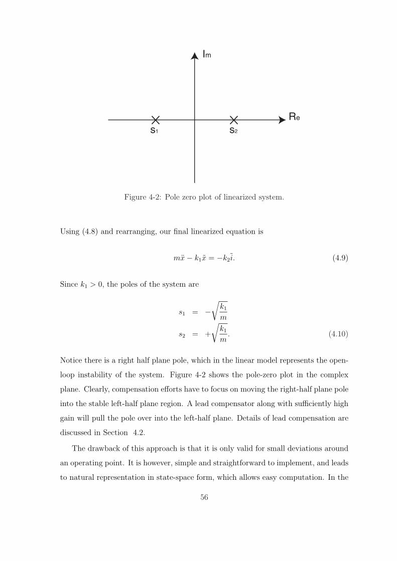
Figure 4-3: Block diagram of system showing nonlinear and linear compensation.

next section we consider another method that overcomes the limitations of traditional

linearization of the plant model.

4.2 Feedback Linearization

The fundamental idea behind feedback linearization is to perform a nonlinear trans-

formation under which the system is mapped to a linear system. A general viewpoint

on the issues of nonlinear control is given in [7] and [8]. The application of such

techniques to magnetic suspensions is discussed in [10] and [11]. The transformation

is intended to be valid over the entire operating range. We then design a controller

using the usual linear feedback techniques. Here, software carries out the nonlinear

transformation. It is possible to implement the operation in analog hardware but

nonlinear operations in such hardware are more difficult to implement.

In its most basic form, the closed loop system has 3 main elements: the linear

compensation, nonlinear compensation, and plant. Figure 4-3 is a conceptual block

diagram representation of this system. The force exhibits a nonlinear relationship

with the current and the function of the nonlinear block is to make the non-linearity

look linear over all operating points. Traditional linear compensation techniques are

then valid to stabilize and enhance performance in the rest of the loop.

We drive the actuator in this system with a current drive amplifier so as to elim-

inate inductance and back emf from the dynamics, and so we perform the transfor-

57

mation on this variable. Solving for the current from (4.6) gives

iset = x

√Fd

C. (4.11)

The current command to the power amplifier varies given a desired force and

position measurement. Based on this algebraic operation to the extent that the

model (4.2) is accurate, the suspension is globally linearized. The inputs to the

nonlinear compensation block are the desired force Fd and the measured position

x. The combination of the nonlinear block and plant now looks linear to the linear

compensation block. The job of the linear block is to specify the variable Fd based

on the difference between the reference and measured position. The nonlinear block

takes Fd as an input and outputs the corresponding set point current to produce the

desired force on the ball. If everything works correctly, the nonlinear compensator

block and plant together have the transfer function

X(s)

F (s)=

1

ms2, (4.12)

where m = 0.067 kg. The resulting block diagram is shown in Figure 4-4. The minus

sign under the square root in the transformation results from the definition of x as

the air gap, and since the magnet force points in the −x direction. Therefore, a

−Fd would drive the coil with positive current (the current drive has inverting gain),

pulling the ball up, and decreasing x. The algebraic operation is in software, the

current drive in hardware, and finally there is the suspension itself: collectively they

are modeled by (4.12).

The linearized system from Fd to x has two poles at the origin making it marginally

stable. In actuality, the poles may be slightly offset from the origin set apart in the

direction of where the poles are is shown in Figure 4-2. The more accurate the

transformation, the closer the poles are to overlaying on the origin. Assuming our

modeling is precise, we must now address the issue of stability by designing the

controller to move these poles off the origin fully into the left-half plane.

58

Linear

Compensator

Position

Transducer

dF

act C-i=-x

dFrefX

Current Drive SuspensionactX-i

2

1

ms

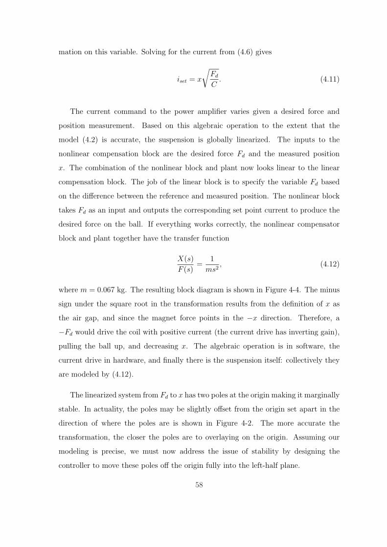
Figure 4-4: Block diagram showing nonlinear transformation.

A lead compensator has the form

Gc(s) = K(ατs + 1). (4.13)

The uncompensated plant has zero phase margin (phase is −180 for all frequencies).

Lead compensation adds phase in the neighborhood of the crossover frequency by

taking advantage of the fact that by the time phase has increased by 45, magnitude

has only increased by√

2 (see Figure 4-5). The network has a low frequency zero

followed by a higher frequency pole. Therefore, when the phase from the zero starts

to take effect the magnitude has not yet begun to rise significantly, and it is possible

to leave the crossover frequency unchanged.

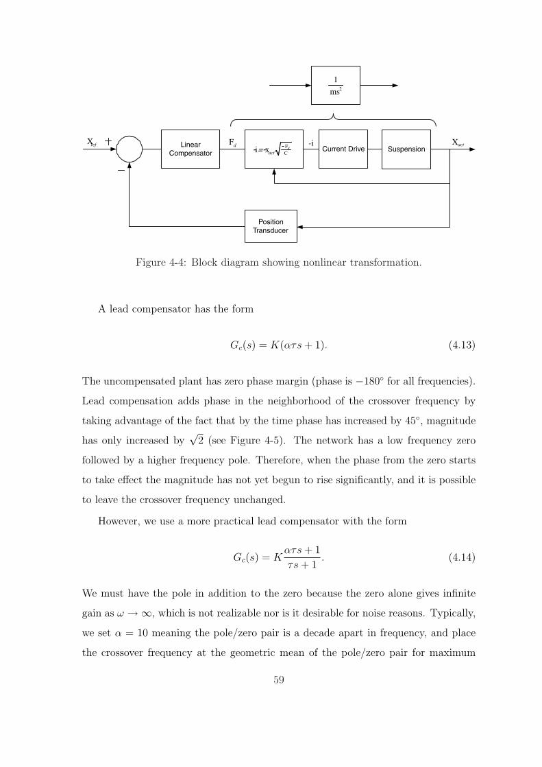
However, we use a more practical lead compensator with the form

Gc(s) = Kατs + 1

τs + 1. (4.14)

We must have the pole in addition to the zero because the zero alone gives infinite

gain as ω →∞, which is not realizable nor is it desirable for noise reasons. Typically,

we set α = 10 meaning the pole/zero pair is a decade apart in frequency, and place

the crossover frequency at the geometric mean of the pole/zero pair for maximum

59

Bode Diagram

Frequency (rad/sec)

Pha

se (

deg)

Mag

nitu

de (

dB)

100

101

102

0

30

60

90

System: sys Frequency (rad/sec): 20 Phase (deg): 45

35

40

45

50

55

System: sys Frequency (rad/sec): 20 Magnitude (dB): 41.1

System: sys Frequency (rad/sec): 1.36 Magnitude (dB): 38.1

Figure 4-5: Bode plot of transfer function Gc(s) = K(ατs + 1) with K = 80, α = 10,and τ = 0.005. This shows the phase has already increased by 45 while magnitudehas only increased by

√2. However, this transfer function is not realizable and a pole

must be added to level off the gain at higher frequencies.

phase improvement. The maximum phase is given by

φm = sin−1 α− 1

α + 1. (4.15)

The Bode plot of a practical lead compensator is shown in Figure 4-6.

The lead compensator will move the poles into the left-half plane but we must

properly choose the parameters to achieve desired performance. For a first cut design

we chose a conservative 10 Hz. Assuming we have done the feedback linearization

accurately, the transfer function of the compensated plant is given by (4.12) and the

60

Bode Diagram

Frequency (rad/sec)

Pha

se (

deg)

Mag

nitu

de (

dB)

35

40

45

50

55

60

100

101

102

103

0

30

60

Figure 4-6: Bode plot of transfer function Gc(s) = K ατs+1τs+1

, a practicial lead networkwith maximum phase at the geometric mean of the pole and zero pair (K = 80, α =10, and τ = 0.005 sec). The bottom plot shows the characteristic phase “bump” of alead compensator.

61

Bode Diagram

Frequency (rad/sec)

Pha

se (

deg)

Mag

nitu

de (

dB)

−100

−50

0

50

100

10−1

100

101

102

−181

−180.5

−180

−179.5

−179

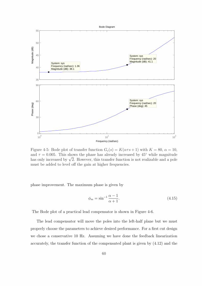
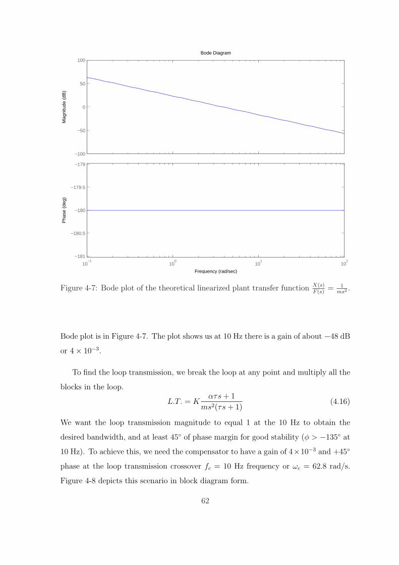
Figure 4-7: Bode plot of the theoretical linearized plant transfer function X(s)F (s)

= 1ms2 .

Bode plot is in Figure 4-7. The plot shows us at 10 Hz there is a gain of about −48 dB

or 4× 10−3.

To find the loop transmission, we break the loop at any point and multiply all the

blocks in the loop.

L.T. = Kατs + 1

ms2(τs + 1)(4.16)

We want the loop transmission magnitude to equal 1 at the 10 Hz to obtain the

desired bandwidth, and at least 45 of phase margin for good stability (φ > −135 at

10 Hz). To achieve this, we need the compensator to have a gain of 4×10−3 and +45

phase at the loop transmission crossover fc = 10 Hz frequency or ωc = 62.8 rad/s.

Figure 4-8 depicts this scenario in block diagram form.

62

3

4 x 10 Xref

X 45

-34 x 10 180

Linear

CompensatorPlant

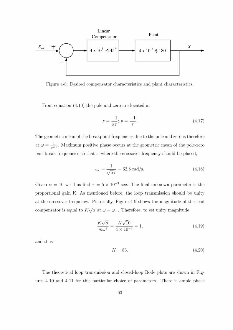
Figure 4-8: Desired compensator characteristics and plant characteristics.

From equation (4.10) the pole and zero are located at

z =−1

ατ; p =

−1

τ. (4.17)

The geometric mean of the breakpoint frequencies due to the pole and zero is therefore

at ω = 1√ατ

. Maximum positive phase occurs at the geometric mean of the pole-zero

pair break frequencies so that is where the crossover frequency should be placed,

ωc =1√ατ

= 62.8 rad/s. (4.18)

Given α = 10 we thus find τ = 5 × 10−3 sec. The final unknown parameter is the

proportional gain K. As mentioned before, the loop transmission should be unity

at the crossover frequency. Pictorially, Figure 4-9 shows the magnitude of the lead

compensator is equal to K√

α at ω = ωc . Therefore, to set unity magnitude

K√

α

mω2=

K√

10

4× 10−3= 1, (4.19)

and thus

K = 83. (4.20)

The theoretical loop transmission and closed-loop Bode plots are shown in Fig-

ures 4-10 and 4-11 for this particular choice of parameters. There is ample phase

63

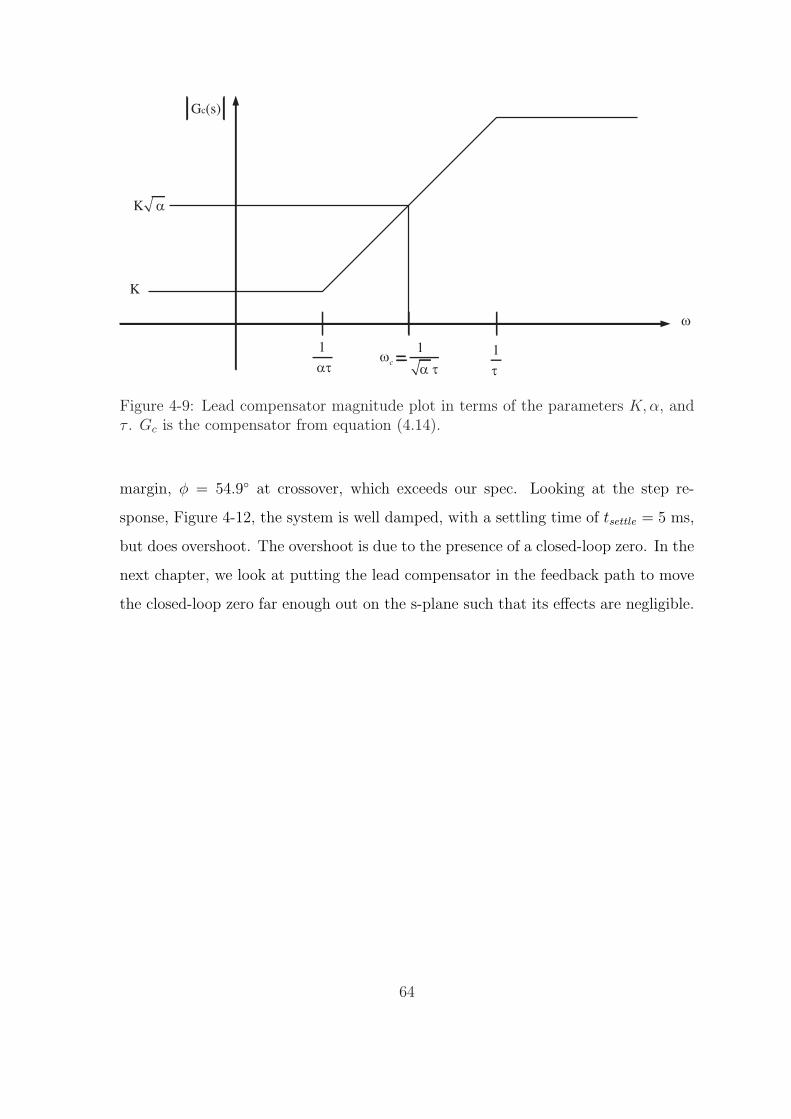
K

K

1

1c

1

Gc(s)

Figure 4-9: Lead compensator magnitude plot in terms of the parameters K,α, andτ . Gc is the compensator from equation (4.14).

margin, φ = 54.9 at crossover, which exceeds our spec. Looking at the step re-

sponse, Figure 4-12, the system is well damped, with a settling time of tsettle = 5 ms,

but does overshoot. The overshoot is due to the presence of a closed-loop zero. In the

next chapter, we look at putting the lead compensator in the feedback path to move

the closed-loop zero far enough out on the s-plane such that its effects are negligible.

64

Bode Diagram

Frequency (rad/sec)

Pha

se (

deg)

Mag

nitu

de (

dB)

−40

−20

0

20

40

60

80Gm = Inf, Pm = 54.9 deg (at 62.247 rad/sec)

100

101

102

103

−180

−150

−120

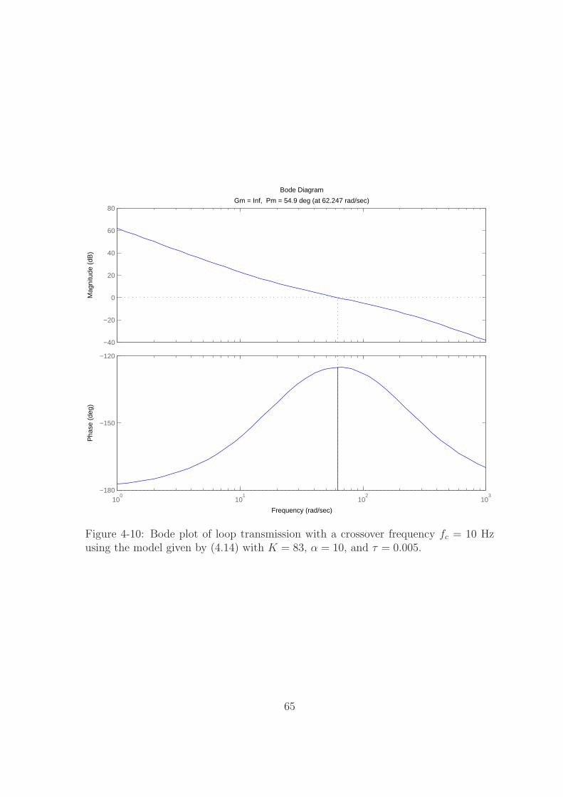
Figure 4-10: Bode plot of loop transmission with a crossover frequency fc = 10 Hzusing the model given by (4.14) with K = 83, α = 10, and τ = 0.005.

65

Bode Diagram

Frequency (rad/sec)

Pha

se (

deg)

Mag

nitu

de (

dB)

101

102

103

−180

−135

−90

−45

0

−60

−50

−40

−30

−20

−10

0

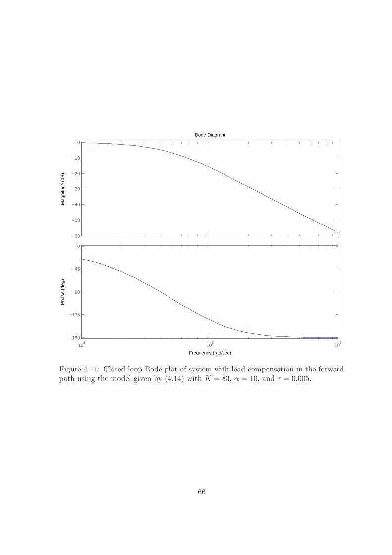
Figure 4-11: Closed loop Bode plot of system with lead compensation in the forwardpath using the model given by (4.14) with K = 83, α = 10, and τ = 0.005.

66

Step Response

Time (sec)

Am

plitu

de

0 0.02 0.04 0.06 0.08 0.1 0.120

0.2

0.4

0.6

0.8

1

1.2

1.4

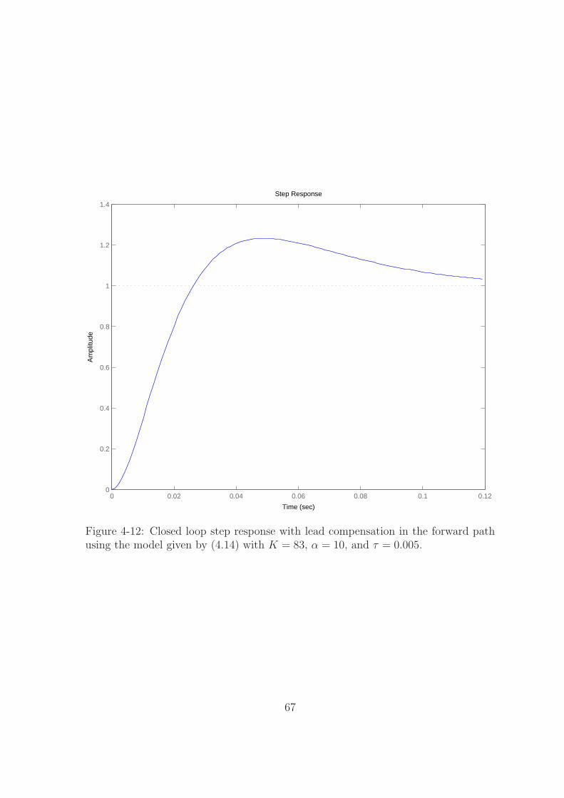
Figure 4-12: Closed loop step response with lead compensation in the forward pathusing the model given by (4.14) with K = 83, α = 10, and τ = 0.005.

67

68

Chapter 5

Design Issues and Results

5.1 Implemented Loop

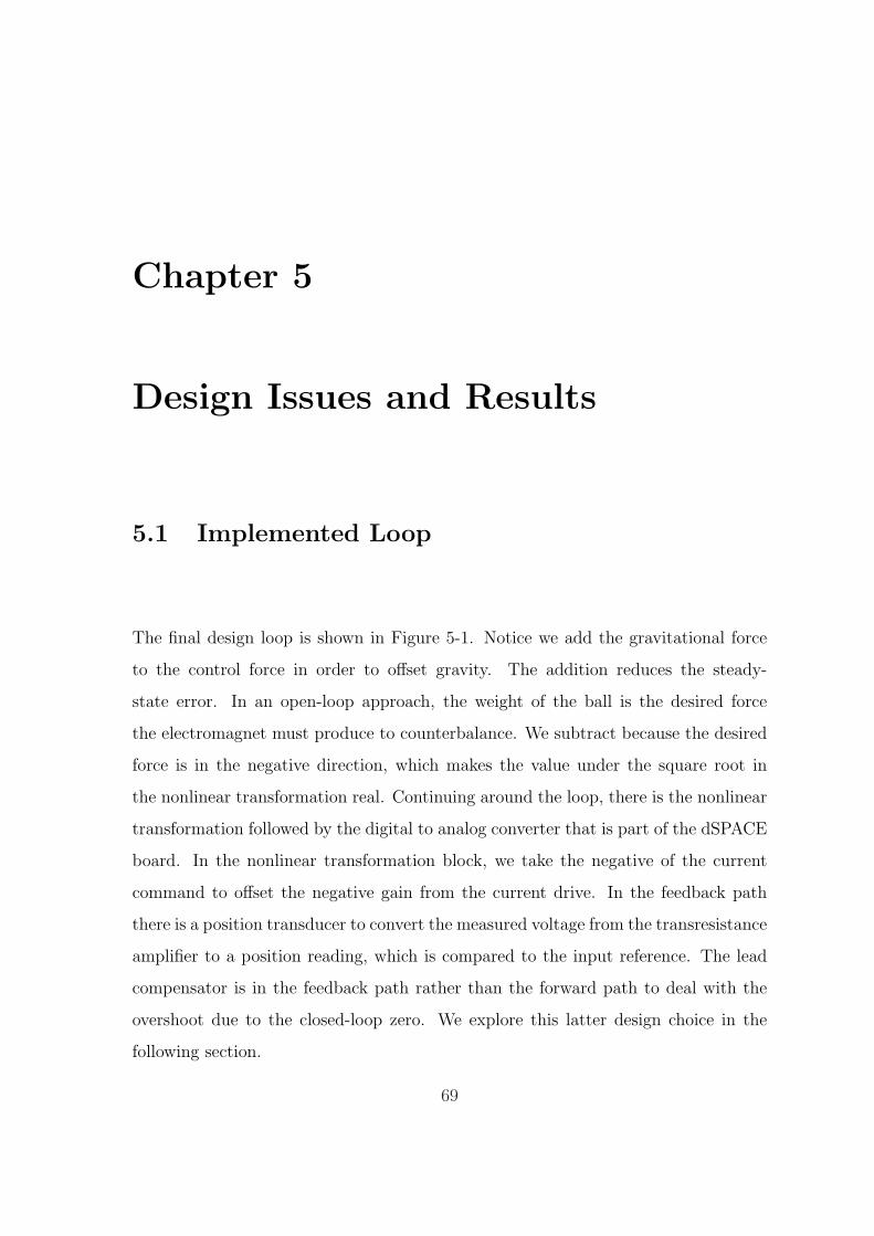
The final design loop is shown in Figure 5-1. Notice we add the gravitational force

to the control force in order to offset gravity. The addition reduces the steady-

state error. In an open-loop approach, the weight of the ball is the desired force

the electromagnet must produce to counterbalance. We subtract because the desired

force is in the negative direction, which makes the value under the square root in

the nonlinear transformation real. Continuing around the loop, there is the nonlinear

transformation followed by the digital to analog converter that is part of the dSPACE

board. In the nonlinear transformation block, we take the negative of the current

command to offset the negative gain from the current drive. In the feedback path

there is a position transducer to convert the measured voltage from the transresistance

amplifier to a position reading, which is compared to the input reference. The lead

compensator is in the feedback path rather than the forward path to deal with the

overshoot due to the closed-loop zero. We explore this latter design choice in the

following section.

69

Positio

n

Sensor

dF

ref

xact

x

Lead

Com

pensato

r

Gain

2

1

Ms

A/DD

/A

mg

mg

Positio

n

Tra

nsducer

Curr

ent D

rive

1

physic

al

hard

ware

dF

act

C-i=

-x

co

ntr

olle

r

fo

rce

Figure 5-1: Block diagram of the closed loop design.

70

Root Locus

Real Axis

Ima

g A

xis

200 180 160 140 120 100 80 60 40 20 0

200

150

100

50

0

50

100

150

200

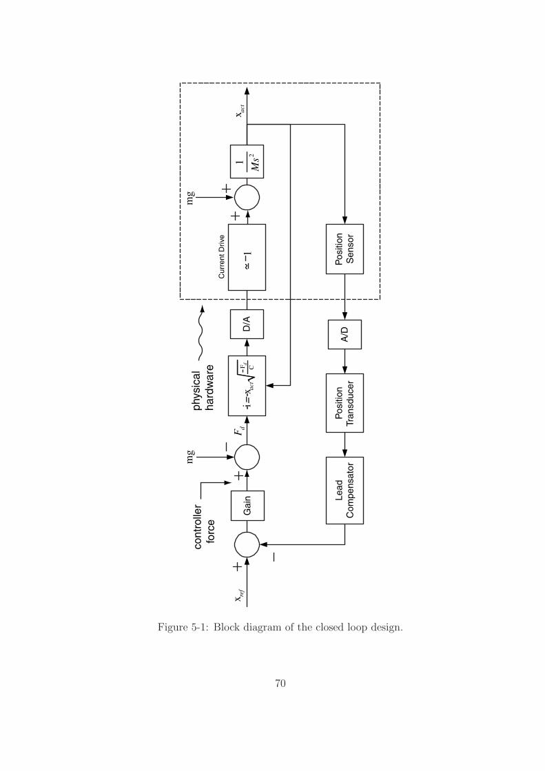
Figure 5-2: Root locus plot of suspension system with lead compensation.

71

5.2 Lead Compensator in the Feedback Path

As mentioned in Chapter 4, there is overshoot seen in the step response. This over-

shoot is due to a closed-loop zero. Looking at the root locus plot in Figure 5-2, we

see as the gain increases, the two poles at the origin leave the real axis, circle around

the zero, reunite on the real axis, and then split again. One of the poles moves to-

wards the zero from the lead compensator. With K = 83 for the 10Hz bandwidth,

Figure 5-3 shows the close loop pole locations. The zero causes the overshoot as seen

in Figure 4-12 in the step response. One way to deal with this problem is to put

the lead network in the feedback path rather than the forward path. Putting the

compensator in the feedback path does not change the loop transmission. However,

poles in the feedback path become zeros in the closed loop system. This is desirable

because the lead compensator pole is at a higher frequency than the zero; thus, the

closed-loop zero is now at 200 rad/s, the dynamics of which are fast enough to ignore.

The resulting step response is shown in Figure 5-5. The response is now well damped,

and there is no overshoot.

Recall the placement of the compensator pole was determined in part by α. With

α = 10, we have maximum positive phase. However, by moving the pole out to a

higher frequency, and thereby giving up some phase margin, the closed-loop dynamics

speed up. Therefore, we give up some phase margin as a tradeoff for a faster rise time.

By a root-locus argument, as the closed-loop zero moves farther to the left on the

s-plane, the poles will move accordingly with increasing open-loop gain.

5.3 Layout Issues

The suspension system in its final form has three main physical components: the

computer (we use a laptop for portability) and accompanying dSPACE boxes, the

power supply and circuitry box, and the suspension structure itself. Figure 5-6 is a

photograph of the all the hardware required for this demo.

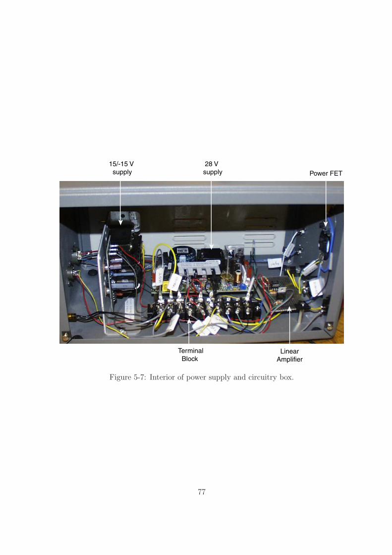
Figure 5-7 shows the interior of the finished power supply and circuitry box. The

72

Pole−Zero Map

Real Axis

Imag

Axi

s

−100 −80 −60 −40 −20 0−8

−6

−4

−2

0

2

4

6

8

Figure 5-3: Pole-zero plot with lead compensator in the forward path. There is a lowfrequency zero that effects the dynamics causing an overshoot in the step response.

73

Pole−Zero Map

Real Axis

Imag

Axi

s

−200 −150 −100 −50 0 50−8

−6

−4

−2

0

2

4

6

8

Figure 5-4: Pole-zero plot with lead compensator in the feedback path. Placing thecompensator in the feedback path moves the zero to −200 rad/s, the location ofthe open loop compensator pole. With the zero at this frequency, the dynamics aredominated by the low frequency poles.

74

Step Response

Time (sec)

Am

plitu

de

0 0.02 0.04 0.06 0.08 0.1 0.120

0.2

0.4

0.6

0.8

1

1.2

1.4

forward path

feedback path

Figure 5-5: Step response of closed loop system with compensator in the feedbackpath. The step response with the compensator in the forward path is overlayed forcomparison. The rise time is faster with the compensator in the forward path buthas overshoot. Settling time is about the same for both.

75

Figure 5-6: Hardware for maglev demo.

inside of the box contains the power supplies, linear amplifier, a storage area for

extra parts, and a connector strip. Appendix B details the design layout for the box.

Also, see Appendix E for a list of vendors and parts. For the 28 V supply we use

a switching supply to accommodate the higher current levels. The switching supply

has lower power dissipation than an equivalent linear supply. For the ±15 V, a linear

supply is sufficient; currents are on the order of 15 mA so even with static loss, power

consumption is not significant.

In the front of the box are two receptacles that connect to the position sensor and

inductor coil - they are of different sizes so the connections are unique. The rear of

the box has a power cord that plugs into a 120 VAC wall socket. In addition, there

are two BNC connections, one to the dSPACE box Vin1, with the sensor signal and

one from the box Vout1, with the command to the amplifier.

One issue that needs attention pertaining to practical implementation is the layout

76

15/-15 V

supply

28 V

supply

Linear

Amplifier

Power FET

Terminal

Block

Figure 5-7: Interior of power supply and circuitry box.

77

ControlCircuitry

PowerCircuitry

1i

2i

1i

2i

i≈ 0 i≈ 0

Figure 5-8: Separation of control and power circuitry.

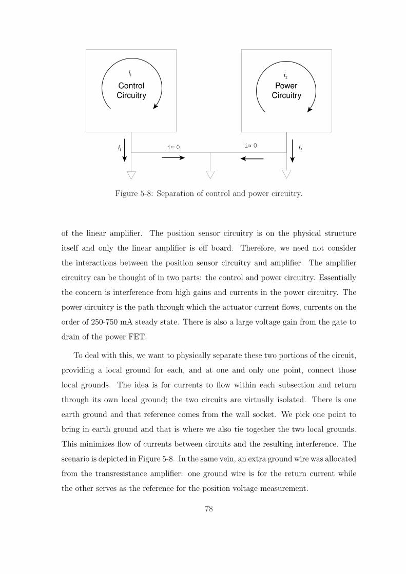
of the linear amplifier. The position sensor circuitry is on the physical structure

itself and only the linear amplifier is off board. Therefore, we need not consider

the interactions between the position sensor circuitry and amplifier. The amplifier

circuitry can be thought of in two parts: the control and power circuitry. Essentially

the concern is interference from high gains and currents in the power circuitry. The

power circuitry is the path through which the actuator current flows, currents on the

order of 250-750 mA steady state. There is also a large voltage gain from the gate to

drain of the power FET.

To deal with this, we want to physically separate these two portions of the circuit,

providing a local ground for each, and at one and only one point, connect those

local grounds. The idea is for currents to flow within each subsection and return

through its own local ground; the two circuits are virtually isolated. There is one

earth ground and that reference comes from the wall socket. We pick one point to

bring in earth ground and that is where we also tie together the two local grounds.

This minimizes flow of currents between circuits and the resulting interference. The

scenario is depicted in Figure 5-8. In the same vein, an extra ground wire was allocated

from the transresistance amplifier: one ground wire is for the return current while

the other serves as the reference for the position voltage measurement.

78

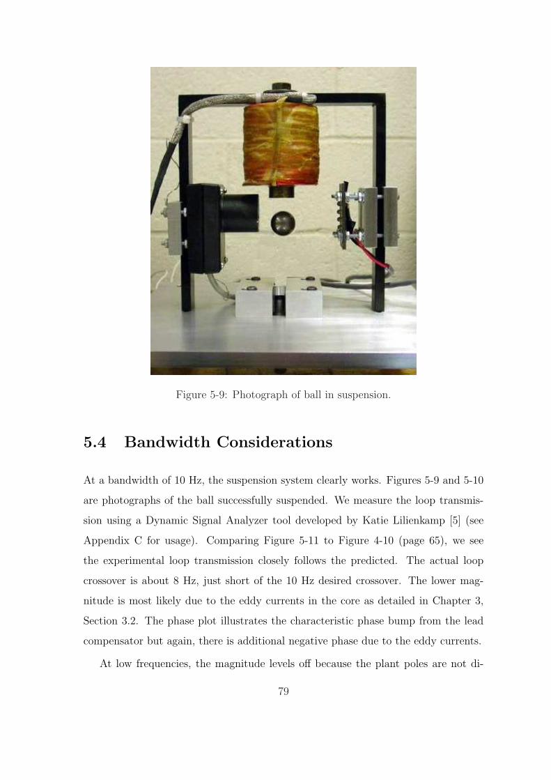
Figure 5-9: Photograph of ball in suspension.

5.4 Bandwidth Considerations

At a bandwidth of 10 Hz, the suspension system clearly works. Figures 5-9 and 5-10

are photographs of the ball successfully suspended. We measure the loop transmis-

sion using a Dynamic Signal Analyzer tool developed by Katie Lilienkamp [5] (see

Appendix C for usage). Comparing Figure 5-11 to Figure 4-10 (page 65), we see

the experimental loop transmission closely follows the predicted. The actual loop

crossover is about 8 Hz, just short of the 10 Hz desired crossover. The lower mag-

nitude is most likely due to the eddy currents in the core as detailed in Chapter 3,

Section 3.2. The phase plot illustrates the characteristic phase bump from the lead

compensator but again, there is additional negative phase due to the eddy currents.

At low frequencies, the magnitude levels off because the plant poles are not di-

79

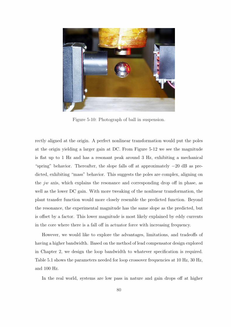
Figure 5-10: Photograph of ball in suspension.

rectly aligned at the origin. A perfect nonlinear transformation would put the poles

at the origin yielding a larger gain at DC. From Figure 5-12 we see the magnitude

is flat up to 1 Hz and has a resonant peak around 3 Hz, exhibiting a mechanical

“spring” behavior. Thereafter, the slope falls off at approximately −20 dB as pre-

dicted, exhibiting “mass” behavior. This suggests the poles are complex, aligning on

the jw axis, which explains the resonance and corresponding drop off in phase, as

well as the lower DC gain. With more tweaking of the nonlinear transformation, the

plant transfer function would more closely resemble the predicted function. Beyond

the resonance, the experimental magnitude has the same slope as the predicted, but

is offset by a factor. This lower magnitude is most likely explained by eddy currents

in the core where there is a fall off in actuator force with increasing frequency.

However, we would like to explore the advantages, limitations, and tradeoffs of

having a higher bandwidth. Based on the method of lead compensator design explored

in Chapter 2, we design the loop bandwidth to whatever specification is required.

Table 5.1 shows the parameters needed for loop crossover frequencies at 10 Hz, 30 Hz,

and 100 Hz.

In the real world, systems are low pass in nature and gain drops off at higher

80

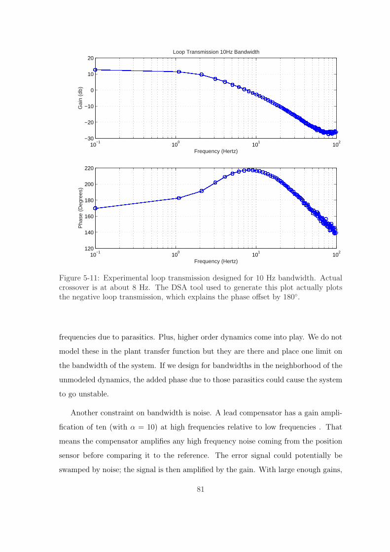
10−1

100

101

102

−30

−20

−10

0

10

20

Frequency (Hertz)

Gai

n (d

b)

Loop Transmission 10Hz Bandwidth

10−1

100

101

102

120

140

160

180

200

220

Frequency (Hertz)

Pha

se (

Deg

rees

)

Figure 5-11: Experimental loop transmission designed for 10 Hz bandwidth. Actualcrossover is at about 8 Hz. The DSA tool used to generate this plot actually plotsthe negative loop transmission, which explains the phase offset by 180.

frequencies due to parasitics. Plus, higher order dynamics come into play. We do not

model these in the plant transfer function but they are there and place one limit on

the bandwidth of the system. If we design for bandwidths in the neighborhood of the

unmodeled dynamics, the added phase due to those parasitics could cause the system

to go unstable.

Another constraint on bandwidth is noise. A lead compensator has a gain ampli-

fication of ten (with α = 10) at high frequencies relative to low frequencies . That

means the compensator amplifies any high frequency noise coming from the position

sensor before comparing it to the reference. The error signal could potentially be

swamped by noise; the signal is then amplified by the gain. With large enough gains,

81

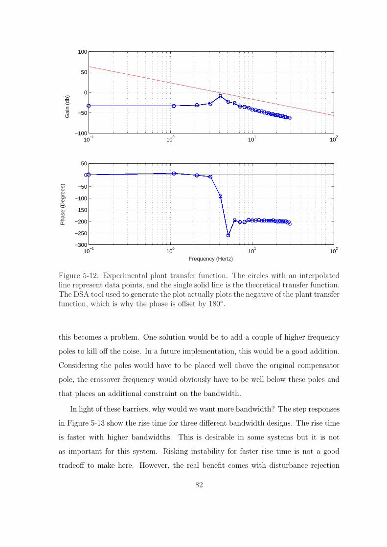
10−1

100

101

102

−100

−50

0

50

100

Gai

n (d

b)

10−1

100

101

102

−300

−250

−200

−150

−100

−50

0

50

Frequency (Hertz)

Pha

se (

Deg

rees

)

Figure 5-12: Experimental plant transfer function. The circles with an interpolatedline represent data points, and the single solid line is the theoretical transfer function.The DSA tool used to generate the plot actually plots the negative of the plant transferfunction, which is why the phase is offset by 180.

this becomes a problem. One solution would be to add a couple of higher frequency

poles to kill off the noise. In a future implementation, this would be a good addition.

Considering the poles would have to be placed well above the original compensator

pole, the crossover frequency would obviously have to be well below these poles and

that places an additional constraint on the bandwidth.

In light of these barriers, why would we want more bandwidth? The step responses

in Figure 5-13 show the rise time for three different bandwidth designs. The rise time

is faster with higher bandwidths. This is desirable in some systems but it is not

as important for this system. Risking instability for faster rise time is not a good

tradeoff to make here. However, the real benefit comes with disturbance rejection

82

fc ωc K τ10 Hz 63 rad/s 83 5 ms30 Hz 126 rad/s 333 2.5 ms100 Hz 628 rad/s 8319 0.5 ms

Table 5.1: Parameters for designing a controller at different bandwidths at 10Hz,30Hz, and 100Hz.

and that is important. Essentially, the higher gain and bandwidth means the system

reacts faster to disturbances. The rise time and disturbance rejection go hand in hand

because both are due to a higher gain.

In an analysis of the position to disturbance force transfer function, we see the

rejection improves with larger gains.

X(s)

Fd(s)=

ms2(τs + 1)

ms2 + K(ατs + 1)

By the final value theorem, x(∞) due to a unit step in disturbance is

x(∞) =1

K. (5.1)

The gain term appears in the denominator so for larger gains, the output due to

disturbance force becomes a smaller fraction. Intuitively, this makes sense because

the error signal is multiplied by the gain but the disturbance is not. Therefore, the

output due to the reference is large in comparison to that due to the disturbance, and

this difference grows with larger gains. Mechanically, a larger K value is equivalent to

making the system stiffer. Figure 5-14 shows two traces, 10 Hz and 30 Hz crossover

designs, of the output due to a step in disturbance force. The disturbance force

contributes a much larger portion to the output in the 10 Hz bandwidth design as

shown by the larger step in response. By inspection, the 30 Hz design has about 4

times better rejection, which verifies (5.1) with K = 83 and K = 333 for the 10 Hz

and 30 Hz bandwidth designs respectively.

Therefore, we win in terms of better rejection of disturbances at higher band-

widths, but at the risk of unmodeled characteristics causing problems. The lesson

83

0 0.01 0.02 0.03 0.04 0.05 0.060

0.2

0.4

0.6

0.8

1

1.2

1.4From: U(1)

To:

Y(1

)

10Hz30Hz100Hz

Figure 5-13: Theoretical step responses for 10, 30, and 100 Hz bandwidth designs.

84

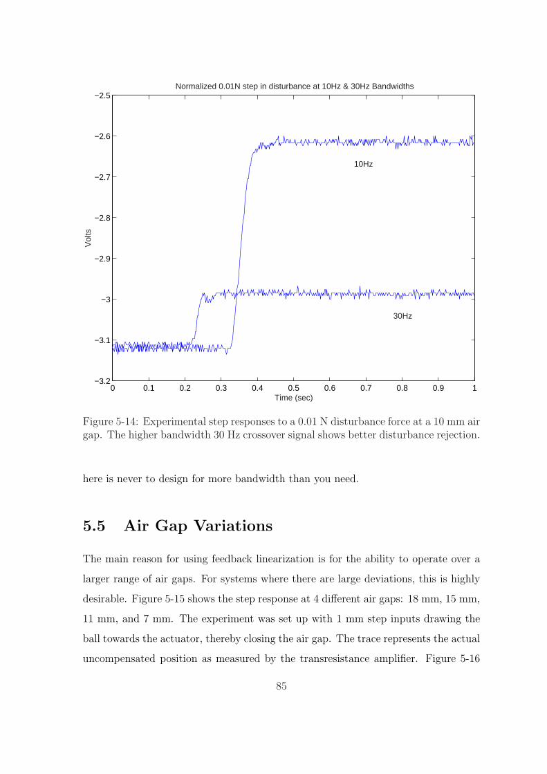
0 0.1 0.2 0.3 0.4 0.5 0.6 0.7 0.8 0.9 1−3.2

−3.1

−3

−2.9

−2.8

−2.7

−2.6

−2.5

10Hz

30Hz

Normalized 0.01N step in disturbance at 10Hz & 30Hz BandwidthsV

olts

Time (sec)

Figure 5-14: Experimental step responses to a 0.01 N disturbance force at a 10 mm airgap. The higher bandwidth 30 Hz crossover signal shows better disturbance rejection.

here is never to design for more bandwidth than you need.

5.5 Air Gap Variations

The main reason for using feedback linearization is for the ability to operate over a

larger range of air gaps. For systems where there are large deviations, this is highly

desirable. Figure 5-15 shows the step response at 4 different air gaps: 18 mm, 15 mm,

11 mm, and 7 mm. The experiment was set up with 1 mm step inputs drawing the

ball towards the actuator, thereby closing the air gap. The trace represents the actual

uncompensated position as measured by the transresistance amplifier. Figure 5-16

85

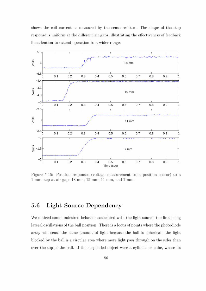
shows the coil current as measured by the sense resistor. The shape of the step

response is uniform at the different air gaps, illustrating the effectiveness of feedback

linearization to extend operation to a wider range.

0 0.1 0.2 0.3 0.4 0.5 0.6 0.7 0.8 0.9 1−6.5

−6

−5.5

Vol

ts

18 mm

0 0.1 0.2 0.3 0.4 0.5 0.6 0.7 0.8 0.9 1−5

−4.8

−4.6

−4.4

Vol

ts

15 mm

0 0.1 0.2 0.3 0.4 0.5 0.6 0.7 0.8 0.9 1−3.5

−3

−2.5

Vol

ts

11 mm

0 0.1 0.2 0.3 0.4 0.5 0.6 0.7 0.8 0.9 1−2

−1.5

−1

Vol

ts

7 mm

Time (sec)

Figure 5-15: Position responses (voltage measurement from position sensor) to a1 mm step at air gaps 18 mm, 15 mm, 11 mm, and 7 mm.

5.6 Light Source Dependency

We noticed some undesired behavior associated with the light source, the first being

lateral oscillations of the ball position. There is a locus of points where the photodiode

array will sense the same amount of light because the ball is spherical: the light

blocked by the ball is a circular area where more light pass through on the sides than

over the top of the ball. If the suspended object were a cylinder or cube, where its

86

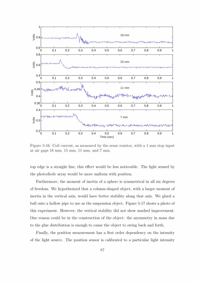
0 0.1 0.2 0.3 0.4 0.5 0.6 0.7 0.8 0.9 10.6

0.8

1

Vol

ts 18 mm

0 0.1 0.2 0.3 0.4 0.5 0.6 0.7 0.8 0.9 10.4

0.6

0.8

Vol

ts 15 mm

0 0.1 0.2 0.3 0.4 0.5 0.6 0.7 0.8 0.9 10.35

0.4

0.45

0.5

Vol

ts

11 mm

0 0.1 0.2 0.3 0.4 0.5 0.6 0.7 0.8 0.9 10.2

0.3

0.4

Vol

ts 7 mm

Time (sec)

Figure 5-16: Coil current, as measured by the sense resistor, with a 1 mm step inputat air gaps 18 mm, 15 mm, 11 mm, and 7 mm.

top edge is a straight line, this effect would be less noticeable. The light sensed by

the photodiode array would be more uniform with position.

Furthermore, the moment of inertia of a sphere is symmetrical in all six degrees

of freedom. We hypothesized that a column-shaped object, with a larger moment of

inertia in the vertical axis, would have better stability along that axis. We glued a

ball onto a hollow pipe to use as the suspension object. Figure 5-17 shows a photo of

this experiment. However, the vertical stability did not show marked improvement.

One reason could be in the construction of the object: the asymmetry in mass due

to the glue distribution is enough to cause the object to swing back and forth.

Finally, the position measurement has a first order dependency on the intensity

of the light source. The position sensor is calibrated to a particular light intensity

87

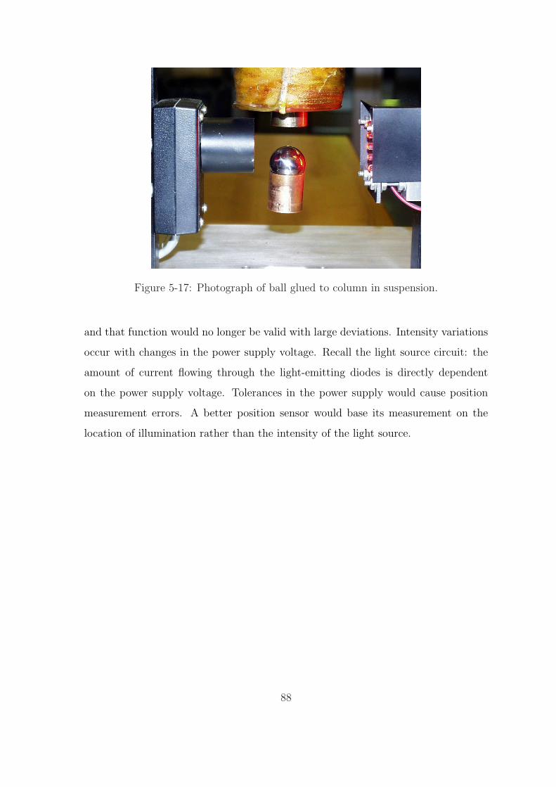
Figure 5-17: Photograph of ball glued to column in suspension.

and that function would no longer be valid with large deviations. Intensity variations

occur with changes in the power supply voltage. Recall the light source circuit: the

amount of current flowing through the light-emitting diodes is directly dependent

on the power supply voltage. Tolerances in the power supply would cause position

measurement errors. A better position sensor would base its measurement on the

location of illumination rather than the intensity of the light source.

88

Chapter 6

Conclusions

6.1 Summary

This thesis presented the design and implementation of a magnetic suspension. The

single-axis suspension system is composed of a position sensor, steel ball, magnetic

coil, linear amplifier, and controller. This classroom demo is an example of a classic

nonlinear controls problem, its development illustrating modeling, dynamics, and

control. We demonstrated the effectiveness of using feedback linearization as a means

of nonlinear control independent of operating point. This is particularly important in

systems where large deviations are expected. However, the system is highly sensitive

to modeling errors. Prior implementations used a switching amplifier; however, we

found a linear amplifier to be sufficient and appropriate because it avoids the noise

generation problems of switched amplifiers. Furthermore, an improvement was made

by using super bright LEDs. The intense, directed light allowed for more accurate

position measurements.

6.2 Suggested Further Work

As outlined in previous research [11], inconsistencies in the light source cause problems

in the nonlinear compensation. Low frequency noise due to a drifty transresistance

amplifier and stray ambient light is likely the main problem. The use of synchronous

89

modulation is a possible solution. As an area for future work, the modulation could

be roughly implemented as follows: the light source is switched on and off at a high

frequency and then synchronous detection is used to sense light only at the switched

frequency, rejecting ambient and other low frequency offsets. When the light source

is switched, the signal is modulated up in the spectrum. The detector receives this

modulated signal along with low frequency noise. The signal along with the noise is

modulated again at the same frequency so that a scaled copy of the desired signal is

centered at its original frequency, while the low frequency noise has been modulated

up. Passing this through a low pass filter gives the desired information. The switched

frequency has to be fast enough to avoid overlapping with the low frequency noise

and to allow sufficiently high control bandwidth.

In addition, it would be desirable to remove the position sensor’s dependency on

absolute intensity as mentioned in Chapter 5. The luminosity of the light source

is dependent on the supply voltage to first order; therefore, slight deviations in the

supply voltages effect the calibration of the position sensor. An alternative would be

a sensor that bases position measurement on location of light rather than its intensity.

Finally, real-world systems need to be robust to modeling errors and process vari-

ations. One problem with feedback linearization is that it is highly dependent on

an accurate model and predictable dynamics. Further work in this area would of

valuable interest for nonlinear controls.

90

Appendix A

Users Guide

One design goal is to make this demo as simple and intuitive as possible from a user’sperspective. The following provides instructions on how to get the suspension systemup and running. The “box” from hereon refers to the box containing the power sup-plies, circuits, etc.

1. Connect the ribbon cable from the dSPACE board to the laptop. Make sure thedongle is connected to the parallel port of the laptop. dSPACE will not run withoutthe dongle.

2. Connect BNC cables to the dSPACE input/output box with the correspondingreceptacles in the back of the box.

3. Connect the cables from the coil, light source, and light sensor to the front ofthe box. Plug the power cord into wall socket.

4. Start Matlab and Simulink. Open the maglev.mdl model and do a build(Ctrl+B). The build should be done in the same directory as the maglev.mdl file.

Push the power button on the back of the box when the demo is ready to run. Suspendthe ball by slowly putting it between the light source and sensor, bringing it up fromthe bottom.

91

92

Appendix B

Box Layout

Below is the physical layout of the power supply and circuitry box. We tried to makethe layout efficient and functional. Aside from the heat sink on the back, only thenecessary connectors are exposed. The storage container built into the box is forextra parts. In the back of the box are the BNC connections to the dSPACE I/Obox. The labels for the BNC connections correspond to the labels on the I/O box(i.e. hook Vin1 to Vin1).

93

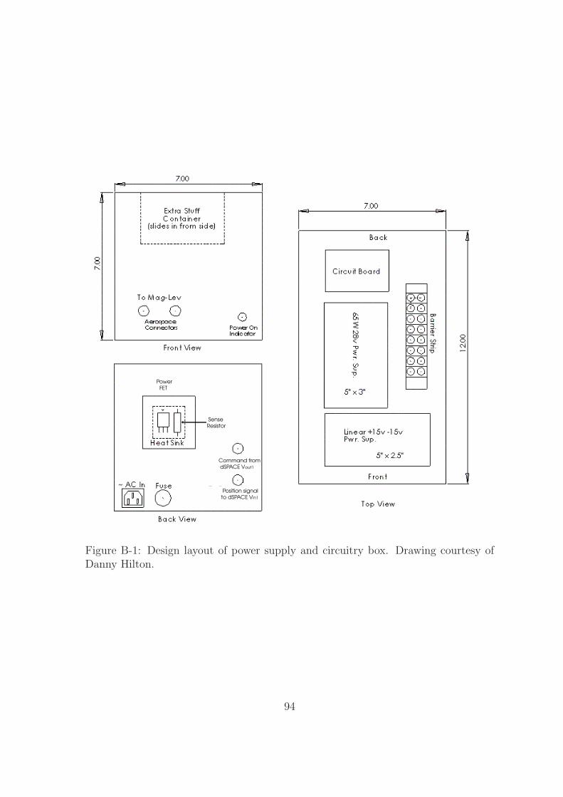
Command from dSPACE Vout1

Position signal to dSPACE Vin1

Power FET

Sense Resistor

Figure B-1: Design layout of power supply and circuitry box. Drawing courtesy ofDanny Hilton.

94

Appendix C

Simulink Models

The following Simulink models were used in testing the suspension system. The firstmodel is used to suspend the ball. The second, uses the Dynamic Signal Analyzertool developed by Katie Lilienkamp to find the loop transmission frequency analysis.The “SineOut” signal is a sine wave that drives the system over a range of frequenciesspecified by running the dsa_1102 script. The “channel1” and “channel2” inputs arethe loop transmission input and output points. In this case, we break the loop atthe error signal and the compensated position signal. See [5] for more details on theDynamic Signal Analyzer tool.

95

0.65

64

mg

Ter

min

ator

3

Ter

min

ator

2

Ter

min

ator

1

.01

Ref

f(u)

Pos

ition

Tra

nsdu

cer

f(u)

Non

linea

rT

rans

form

atio

n

50e-

3s+

1

5e-3

s+1

Lead

Com

pens

atio

n

Gro

und2

Gro

und1

Gro

und

83 Gai

n

DA

C #

1

DA

C #

2

DA

C #

3

DA

C #

4

DS

1102

DA

C

AD

C #

1

AD

C #

2

AD

C #

3

AD

C #

4

DS

1102

AD

C

Err

or

Pos

ition

Cur

rent

Com

man

dF

d

Figure C-1: Simulink model for the magnetic suspension system.

96

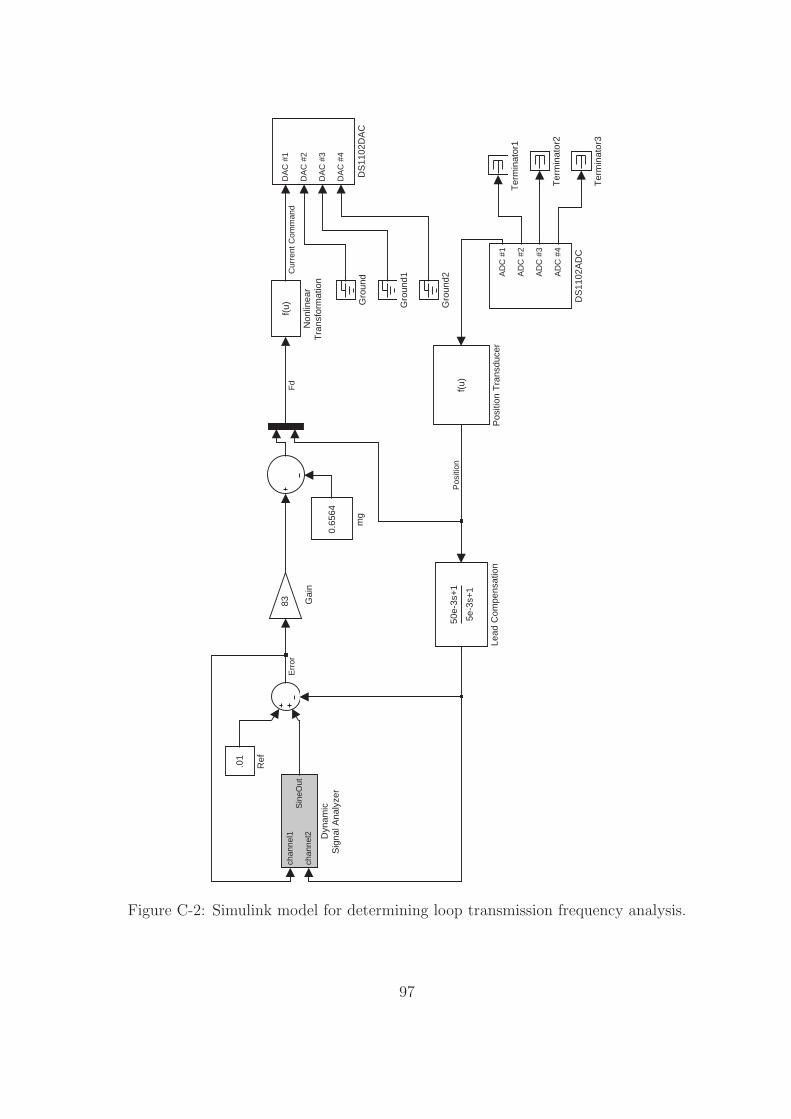
0.65

64

mg

Ter

min

ator

3

Ter

min

ator

2

Ter

min

ator

1

.01

Ref

f(u)

Pos

ition

Tra

nsdu

cer

f(u)

Non

linea

rT

rans

form

atio

n

50e-

3s+

1

5e-3

s+1

Lead

Com

pens

atio

n

Gro

und2

Gro

und1

Gro

und

83 Gai

n

chan

nel1

chan

nel2

Sin

eOut

Dyn

amic

Sig

nal A

naly

zer

DA

C #

1

DA

C #

2

DA

C #

3

DA

C #

4

DS

1102

DA

C

AD

C #

1

AD

C #

2

AD

C #

3

AD

C #

4

DS

1102

AD

C

Pos

ition

Cur

rent

Com

man

dF

dE

rror

Figure C-2: Simulink model for determining loop transmission frequency analysis.

97

98

Appendix D

Matlab Code

D.1 Base Code

This is the base code for family_force_final.m, x0_mean_final.m and C_constant_final.m

. . . all of those files should start with this code.

clear all;

hold on;

%load data and use best

temp = -1; for count=1:11;

temp = temp + 1;

name = ([num2str(count), ’mm’]); %%name file to import

%%files are named by the gap length in mm so we just iterate

%%through them all

load(name);

lgth = 24; %% number of data points

first = 1+ lgth*(temp);

last = 24 + lgth*(temp);

i= trace_y(1,1:49); %%load current and force data points

f = trace_y(2,1:49); %% ’trace_y’ is the var loaded from file

f1 = f(1:24);%%1st part of curve - increasing in value

%%2nd part of curve - flipped so it is also increasing in value

f2 = fliplr(f(26:49));

%f3 = f(101:151) %%other points you can look at

%f4 = fliplr(f(151:201));

xt = i(1:24); %%%current is on the x-axis

99

fmean = mean([f1;f2]); %%take the average of the 2 curves

Xaverage(first: last) = xt; %%stores average of all the curves

%%[i.e. the points in each file added onto the vector

Yaverage(first: last) = fmean;

%%sorts & calculates the interpolated values of all the curves

A =[xt;fmean]’;

A =sortrows(A, 1);%makes sure pts are monotonically increasing

%%important for interp1 function

ft = 1+ 10001*temp; %%number of points in interpolated function

lt = 10001 + 10001*temp;

xx(ft:lt) =0:0.0001:1; %%first column is the current

yy(ft:lt) = interp1(A(:,1), A(:,2), xx(ft:lt));

%%2nd column is the force, interpolated

x(ft:lt) = count*ones(1,10001);

%%3rd column formed by the air gap value

end

100

D.2 Family of Force Curves

File: family_force_final.mCode plots the family of force curves at different air gaps uses a mean average fit forthe hysteresis curves

%%% include base code here %%%%

plot(Xaverage, Yaverage, ’r.’);

title(’Family of force curves over different air gaps’);

ylabel(’Force (N)’);

xlabel(’Current (A)’);

101

D.3 Averaging Hysteresis Curves

File: x0_mean_final.mThis script determines the xO constant in the force equation F = C(i/x + x0)2. Ituses a mean average fit for the hysteresis curves.

%%% include base code here %%%%

%fill variables for a plot of current versus position

force = [0.6 0.61; 1.2 1.21; 2 2.01; 3 3.01];

%%pick out x,i for F=0.6, F=1.2, F=2, F=3

for j=1:4 %%for each force level, plot the current vs. position

count =1;

y = [];

t = [];

for n=1:lt;

if ((yy(n) >= force(j, 1)) & (yy(n) <= force(j, 2)))

y(count) = xx(n);

t(count) = x(n)+.26;

%%offset factor in micrometer measurement

%%(i.e. zero on micrometer is not zero gap)

count = count +1;

end

end

%%%%%%%%%%%%%%%%%%%%%%%%%%%%%%%%%%%%%%%%%%%%%%%%%%%%%%%%%%%%%%%%%%

%use linear best fit to draw family of curves and determine x0

l = length(t);

Xmean = sum(t)/l;

Ymean = sum(y)/l;

Mxy = sum((t-Xmean).*(y-Ymean));

Mxx = sum((t-Xmean).^2);

m = Mxy/Mxx;

b = Ymean-m*Xmean;

tlong = (-8:.1:t(l)); %%extend the x-axis because curves

%%will intersect at x<0

Ytheo=m*tlong +b; %%this is just y=mx+b

plot(t,y,’r.’); %%plot actual points

plot(tlong,Ytheo,’b.’); %%overlay with linear best-fit line

xv0(j) = -b/m; %%vector of x0 constants at each force level

%%gtext([num2str(force(j, 1)),’N’]);

%%uncomment this if you want to label each force

102

end

x0 = (xv0(1) + xv0(2) + xv0(3) + xv0(4))/4; %%average x0 constants

title([’Determining finite reluctance offset x0=’,num2str(x0/1000),

’m’])

xlabel(’X gap in mm’);

ylabel(’Current (A)’);

103

D.4 Determining the C constant

File: C_constant_final.mCode determines the C constant in the force equation F = C(i/x)2 - uses a meanaverage fit for the hysteresis curves.

%%% include base code here %%%

%fill variables for a plot of current versus position

force = [2.8 2.802]; %%picks out values for a fixed F=2.8

count =1;

y = [];

t = [];

for n=1:lt;

if ((yy(n) >= force(1)) & (yy(n) <= force(2)))

%%must give range because number in data are carried out a

%%number of decimal places; yy(n)=force will return false otherwise

y(count) = xx(n); %%current

t(count) = (x(n)+.26)./1000;

%%offset factor in micrometer measurement

%%(i.e. zero on micrometer is not zero gap)

count = count +1;

end

end

%%%%%%%%%%%%%%%%%%%%%%%%%%%%%%%%%%%%%%%%%%%%%%%%%%%%%%%%%%%%%%%%%%

%%calculation of C value

c = (((t+.00364).^2)./(y.^2)).*force(1); %%% c = f*x^2/i^2;

%%plots a linear best-fit based on c values

l = length(y);

Xmean = sum(y)/l;

Ymean = sum(c)/l;

Mxy = sum((y-Xmean).*(c-Ymean));

Mxx = sum((y-Xmean).^2);

m = Mxy/Mxx;

b = Ymean-m*Xmean;

Ytheo=m*y +b;

plot(y,c, ’r.’,y,Ytheo);

title([’C values at f=2.8N Cave=’, num2str(mean(c)*10000),

’x 10^-4 NA^2/m^2’]);

xlabel(’X gap in cm’);

ylabel(’C constant’);

104

D.5 Voltage and Position Calibration

File: sensor_final.mThis script generates a plot of voltage vs. position data points. It interpolates witha linear best-fit.

%input data points of voltage measurements & form position vector

v=-1*[.26 .49 .70 .99 1.36 1.73 2.10 2.51 2.97 3.44 3.91 4.4 4.87

5.33 5.78 6.25 6.70 7.16 7.52];

xg = [0:1:18];

%normalize to meter units and add on offset to micrometer reading

xg = 0.001*(xg+1.44);

%linear best-fit

n = length(xg);

Xmean = sum(xg)/n;

Ymean = sum(v)/n;

Mxy = sum((xg-Xmean).*(v-Ymean));

Mxx = sum((xg-Xmean).^2);

m = Mxy/Mxx;

b = Ymean-m*Xmean;

Ytheo=m*xg +b;

%plot best fit y = mx + b

plot(xg, v, ’mo’, xg, Ytheo);

title([’y = ’, num2str(m), ’x + ’, num2str(b)]);

xlabel(’Position X (m)’);

ylabel(’Voltage V (volts)’);

105

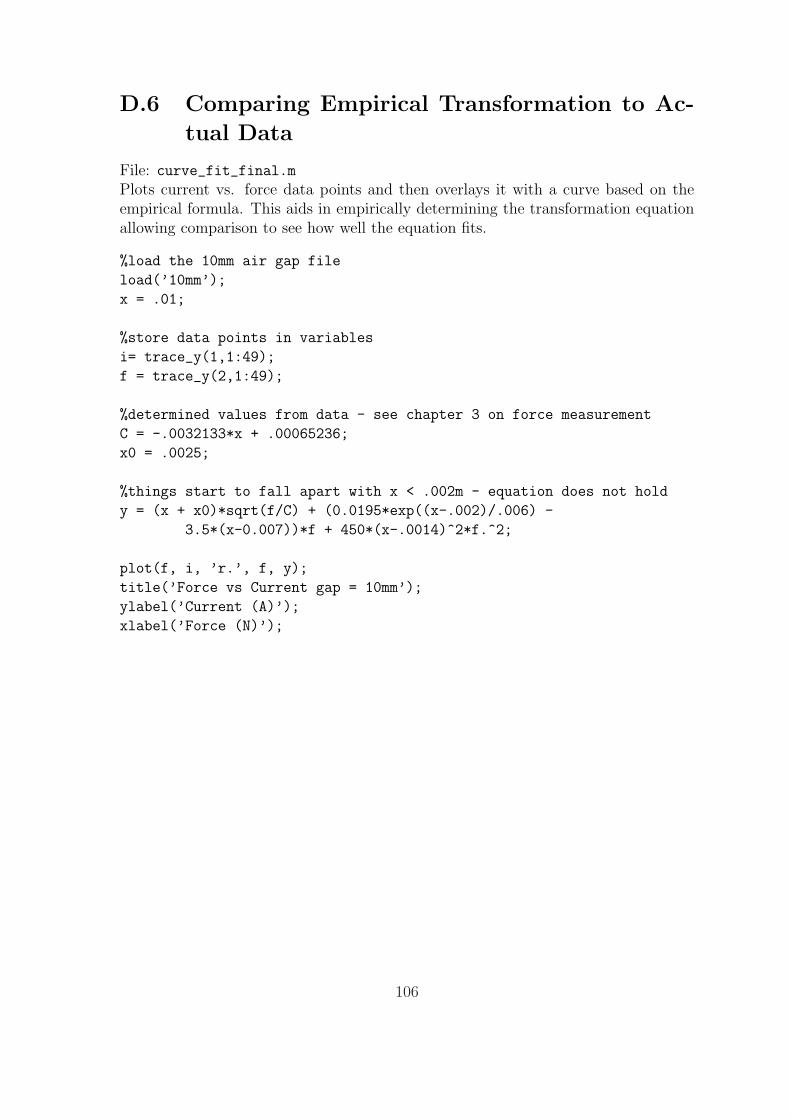
D.6 Comparing Empirical Transformation to Ac-

tual Data

File: curve_fit_final.mPlots current vs. force data points and then overlays it with a curve based on theempirical formula. This aids in empirically determining the transformation equationallowing comparison to see how well the equation fits.

%load the 10mm air gap file

load(’10mm’);

x = .01;

%store data points in variables

i= trace_y(1,1:49);

f = trace_y(2,1:49);

%determined values from data - see chapter 3 on force measurement

C = -.0032133*x + .00065236;

x0 = .0025;

%things start to fall apart with x < .002m - equation does not hold

y = (x + x0)*sqrt(f/C) + (0.0195*exp((x-.002)/.006) -

3.5*(x-0.007))*f + 450*(x-.0014)^2*f.^2;

plot(f, i, ’r.’, f, y);

title(’Force vs Current gap = 10mm’);

ylabel(’Current (A)’);

xlabel(’Force (N)’);

106

Appendix E

Vendors

Amphenol Military/Aerospace Industrial Operations40-60 Delaware AvenueSidney, NY 13838-1395Telephone — (800) 678-0141Web address — http://www.amphenol-aerospace.comProducts used:MS3106F-10SL-3S, MS3106F-16S-1S connector plugs, MS3102R-10SL03P,MS3102R-16S-1P receptacles

Bud Industries, Inc.4605 East 355th StreetWilloughby, Ohio 44094Telephone — (440) 946-3200Web address — http://www.budind.comProduct used: 7.25” x 12.25” x 7.75” enclosure

Condor DC Power Supplies Inc.2311 Statham Pkwy.Oxnard, CA 93033Telephone — (805) 486-4565Web address — http://www.condorpower.comProducts used: ±15 V linear power supply, GLM65-28 28 V switching supply

dSPACE Inc.28700 Cabot Drive – Suite 1100Novi, MI 48377Telephone — (248) 567-1300Web address — http://www.dspaceinc.com/index.htmProduct used: ControlDesk, DS1102 controller board, expansion box, I/O panel

107

The MathWorks, Inc.3 Apple Hill Dr.Natick, MA 01760-2098Telephone — (508) 647-7000Web address — http://www.mathworks.comProducts used: MATLAB, Simulink

108

Bibliography

[1] J. Eric Corban, Anthony J. Calise, J.V.R. Prasad, Jeong Hur, and Nakwan Kim.

Flight evaluation of adaptive high-bandwidth control methods for unmanned

helicopters. AIAA Guidance, Navigation, and Control Conference and Exhibit,

2002.

[2] H. A. Haus and J.R. Melcher. Electromagnetic Fields and Energy. Prentice Hall,

1989.

[3] B. Kadmiry, P. Bergsten, and D. Driankov. Autonomous helicopter control using

fuzzy gain scheduling. Proc. of the IEEE Int. Conf. on Robotic and Automa-

tion(ICRA), 2001.

[4] A.S. Krupadanam, A.M. Annaswamy, and R.S. Mangoubi. A multivariable adap-

tive control design with applications to autonomous helicopters. AIAA Journal

of Guidance, Navigation, and Control, 2002.

[5] K.A. Lilienkamp and D.L. Trumper. Dynamic Signal Analyzer for dSPACE.

Precision Motion Control Lab, MIT, 77 Mass. Ave; Rm. 35-030.

[6] Toru Namerikawa, Masayhuki Fujita, and Roy S. Smith. H∞ control attenuating

initial state uncertainties and its application to the magnetic suspension system.

Proceedings of the Eight International Symposium on Magnetic Bearings, 2002.

[7] Zhihua Qu. Robust Control of Nonlinear Uncertain Systems. John Wiley and

Sons, 1998.

109

[8] Jean-Jacques E. Slotine and Weiping Li. Applied Nonlinear Control. Prentice-

Hall, 1991.

[9] D.L. Trumper. Magnetic Suspension Techniques for Precision Motion Control.

PhD thesis, Massachusetts Institute of Technology, 1990.

[10] D.L. Trumper. Nonlinear compensation techniques for magnetic suspension sys-

tems. NASA Workshop on Aerospace Applications of Magnetic Suspension Tech-

nology, 1990.

[11] D.L. Trumper, J.C. Sanders, T. H. Nguyen, and M.A. Queen. Experimental re-

sults in nonlinear compensation of a one-degree-of-freedom magnetic suspension.

International Symposium on Magnetic Suspension Technology, 1991.

[12] M.C. Weng. Magnetic Suspension and Vibration Control of Flexible Structures

for Non-contact Processing. PhD thesis, Massachusetts Institute of Technology,

2000.

[13] H.H. Woodson and J.R. Melcher. Electromechanical Dynamics - Part I. John

Wiley and Sons, 1968.

110