Embed Size (px)
Citation preview

20/08/2012
Page 1 of 61
Medium-frequency cycles and the remarkable near trend-stationarity of
output.
Tom Holden1, School of Economics, University of Surrey
Abstract: This paper builds a dynamic stochastic general equilibrium (DSGE) model of endogenous
growth that generates large medium-frequency cycles while robustly matching the near trend-
stationary path of observed output. This requires a model in which standard business cycle shocks
lead to highly persistent movements around trend, without significantly altering the trend itself. The
robustness of the trend also requires that we eliminate the scale effects and knife edge assumptions
that plague most growth models. In our model, when products go out of patent protection, the rush
of entry into their production destroys incentives for process improvements. Consequently, old
production processes are enshrined in industries producing non-protected products, and shocks that
affect invention rates change the proportion of industries with advanced technologies. In an
estimated version of our model, a financial-type shock to the stock of ideas emerges as the key
driver of the medium frequency cycle.
Keywords: medium frequency cycles, patent protection, scale effects
JEL Classification: E32, E37, L16, O31, O33, O34
1 Contact address: School of Economics, FBEL, University of Surrey, Guildford, GU2 7XH, England
Contact email: [email protected] Web-site: http://www.tholden.org/
The author would particularly like to thank his supervisor, Simon Wren-Lewis. Further thanks are due to Eric
Bartelsman, Paul Beaudry, Pedro Bento, George Bitsakakis, Ana-Maria Dumitru, Martin Ellison, Fabio Ghironi, Tim
Kehoe, Paul Levine, Omar Licandro, Peter Neary, Joaquim Oliveira Martins, Christopher Nekarda, Walter Park, Pietro
Peretto, James Reade, Diego Restuccia, Nicole Tabasso, David Vines and the participants in numerous seminars at which
versions of this paper were presented. Financial support provided to the author by the ESRC is also greatly appreciated.
The author gratefully acknowledges the use of the Oxford e-Research Centre’s Windows Compute Cluster and the
University of Surrey FBEL cluster for the numerical computations performed in this paper, and the use of data from the
Nuffield College Data Library.

20/08/2012
Page 2 of 61
1. Introduction
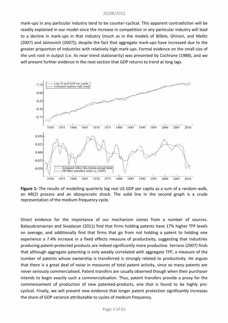
Viewed from a distance, a log-plot of the last one hundred years of US GDP looks very near linear.
However, closer inspection reveals large medium frequency fluctuations around this linear trend.
Generating this combination of remarkably near trend-stationary long run growth and large cycles
around the trend is a challenge for traditional models of endogenous growth. The near linear trend
requires scale effects to be removed not just in the long run, but in the shorter run as well. Models
that remove these scale effects via knife-edge assumptions will usually fail this test, as temporary
business cycle shocks will knock the model away from perfectly removing the scale effect, leading
to a permanent break in the trend of the GDP. Equally, models that remove scale effects via new
product creation will tend to produce such trend breaks in GDP if the stock of new products can
only respond slowly following a shock. On the other hand if the stock of products can adjust
instantly following a shock then (in standard models) there would be no movement in productivity
at all, let alone the large, persistent medium frequency cycles that Comin and Gertler (2006)
document in the data, and that may be seen in our Figure 1 below. In this paper, we present a
mechanism capable of reconciling this apparently contradictory low and medium frequency
behaviour of output, while also matching the cyclicality of mark-ups: the key determinant of
research and invention decisions.
Our story is as follows. The returns to inventing a new product are higher in a boom due to the
higher demand. As a result, during periods of expansion the rate of creation of new products
increases, in line with the evidence of Broda and Weinstein (2010). Due to a first mover advantage,
patent protection, or reverse-engineering difficulties, the inventors of these new products will be
able to extract rents from them, increasing the costs manufacturing firms face if they wish to
produce the new product. These higher costs lead to lower competition in new industries,
increasing mark-ups and thus increasing firms’ incentives to perform the R&D necessary to catch-up
with and surpass the frontier, for basically Schumpeterian reasons. Consequently, the higher
proportion of industries that are relatively new in a boom will lead to higher aggregate productivity,
lower dispersion of both productivity levels and growth rates, as well as higher mark-ups. Since the
length of time for which inventors can extract rents will be determined by the effective duration of
patent-protection, this effect will naturally work at medium frequencies. However, since we allow
both for the creation of new industries (producing new products) and for a varying number of firms
within each industry, even in the short-run the demand faced by any given firm will be roughly
constant, meaning that our model will not produce large deviations from linear growth.
Evidence for the pro-cyclicality of TFP has been presented by Bils (1998) and Campbell (1998)
amongst others, with Comin and Gertler (2006) showing that the evidence is particularly clear at
medium-frequencies. The counter-cyclicality of productivity dispersion has been shown by Kehrig
(2011), with evidence on the counter-cyclicality of the dispersion of productivity growth rates
provided by e.g. Eisfeldt and Rampini (2006) and Bachmann and Bayer (2009). Evidence for the pro-
cyclicality of aggregate mark-ups has been presented by Boulhol (2007) and Nekarda and Ramey
(2010). Nekarda and Ramey also show that mark-ups lead output at business-cycle frequencies, we
will present further evidence in section 2 below that this relationship continues to hold at medium-
frequencies. Boulhol (2007) also shows that although aggregate mark-ups are pro-cyclical, the
20/08/2012
Page 3 of 61
mark-ups in any particular industry tend to be counter-cyclical. This apparent contradiction will be
readily explained in our model since the increase in competition in any particular industry will lead
to a decline in mark-ups in that industry (much as in the models of Bilbiie, Ghironi, and Melitz
(2007) and Jaimovich (2007)), despite the fact that aggregate mark-ups have increased due to the
greater proportion of industries with relatively high mark-ups. Formal evidence on the small size of
the unit root in output (i.e. its near trend stationarity) was presented by Cochrane (1988), and we
will present further evidence in the next section that GDP returns to trend at long lags.
Figure 1: The results of modelling quarterly log real US GDP per capita as a sum of a random walk, an AR(2) process and an idiosyncratic shock. The solid line in the second graph is a crude representation of the medium-frequency cycle.
Direct evidence for the importance of our mechanism comes from a number of sources.
Balasubramanian and Sivadasan (2011) find that firms holding patents have 17% higher TFP levels
on average, and additionally find that firms that go from not holding a patent to holding one
experience a 7.4% increase in a fixed effects measure of productivity, suggesting that industries
producing patent-protected products are indeed significantly more productive. Serrano (2007) finds
that although aggregate patenting is only weakly correlated with aggregate TFP, a measure of the
number of patents whose ownership is transferred is strongly related to productivity. He argues
that there is a great deal of noise in measures of total patent activity, since so many patents are
never seriously commercialised. Patent transfers are usually observed though when their purchaser
intends to begin exactly such a commercialisation. Thus, patent transfers provide a proxy for the
commencement of production of new patented-products, one that is found to be highly pro-
cyclical. Finally, we will present new evidence that longer patent protection significantly increases
the share of GDP variance attributable to cycles of medium frequency.
20/08/2012
Page 4 of 61
Previous papers have introduced endogenous productivity improvement into business cycle models
(e.g. Comin and Gertler (2006), Comin (2009), Comin, Gertler, and Santacreu (2009), Phillips and
Wrase (2006), Nuño (2008; 2009; 2011)), or looked at cycles in growth models (e.g. Bental and
Peled (1996), Matsuyama (1999), Wälde (2005), Francois and Lloyd-Ellis (2008; 2009), Comin and
Mulani (2009)). However, all of these papers have problems with scale effects, either in the long-
run, or in the short-run, and thus all of them would predict counter-factually large unit roots in
output in the presence of standard DSGE shocks. Furthermore, it is not obvious how these scale
effects could be removed without destroying the papers’ mechanisms for generating aggregate TFP
movements. For example, the papers of Wälde (2005) and Phillips and Wrase (2006) rely on there
being a small finite number of sectors. Removing the scale effect would mean allowing this number
to grow over time with population, meaning the variance of productivity would rapidly go to zero.
Indeed, this happens endogenously in the model of Horii (2011). Many models of endogenous
mark-up determination (e.g. Bilbiie, Ghironi, and Melitz (2007) or Jaimovich (2007)) have a similar
problem, with the presence of a small finite number of industries being crucial for explaining the
observed variance of mark-ups. Indeed, Bilbiie, Ghironi, and Melitz (2011) write that “reconciling an
endogenous time-varying markup with stylized growth facts (that imply constant markups and
profit shares in the long run) is a challenge to growth theory”. By disentangling the margins of firm
entry and product creation, we will be able to answer this challenge.
The paper of most relevance to our work is Comin and Gertler (2006), as they made the important
contribution of bringing the significance of medium-frequency cycles to the attention of the
profession. Additionally, their theoretical model, like ours, stresses the effects of mark-up variations
on productivity growth. Unfortunately however, it counter-factually predicts that increases in mark-
ups lead to falls in output, contrary to the empirical evidence of Nekarda and Ramey (2010).
Furthermore, its only major sources of productivity persistence are the persistence of the driving
mark-up shock, and the counter-factual trend break in productivity following such a shock. We
conclude then that the literature still lacks a model of productivity capable of explaining both its
short run and its long run behaviour.
In section 3, we present a model capable of doing this. In order to remove both the long run and
the short run scale effect, as discussed above it will feature a varying number of industries, each of
which will contain a varying number of firms. We do not wish to make any exogenous assumptions
on the differences between industries producing patented products versus those producing
unpatented ones, so in order to match the medium-frequency behaviour of productivity and mark-
ups it is important that our model allow endogenous variation in these quantities across industries.
Were we to assume free transfer of technologies across industries there would be too little
difference in productivity between patent-protected and un-patent-protected industries, and hence
we would not be able to generate medium-frequency cycles. Equally, were we to assume
technology transfer across industries was impossible then it would be legitimate to inquire whether
the difference between these industry types was implausibly large, as perhaps firms in non-
protected industries would find it optimal to perform technology transfer even if they did not find it
optimal to perform any research. Consequently, in modelling the endogenous productivity in each
industry we will allow firms both to perform research, and to perform a costly process of catch-up
to the frontier we shall term appropriation. To make clear the strength of the amplification and

20/08/2012
Page 5 of 61
persistence mechanism presented here, we initially omit capital from the model, and we focus on
the impulse responses to non-persistent shocks when we discuss our model’s qualitative behaviour
in section 4. Finally, in section 5, we add a few standard additional features to the model (habits,
capital with adjustment costs, variable capacity utilisation, sticky wages, Taylor rule monetary
policy) and we show that this model matches the data well at low, medium and high frequencies,
with financial-type shocks to the stock of ideas playing the key role in driving medium-frequency
fluctuations.
2. Empirics
2.1. The near trend stationarity of output
We begin by presenting evidence that GDP returns to trend at long lags. Since statistical tests on
regressions with large numbers of lags tend to suffer from a lack of power, we have to find a
sparsely parameterised way of capturing this long-run behaviour. It seems implausible that a high-
frequency spike in GDP should lead to another spike in GDP many periods later. Instead, if GDP
responds at all to its own past fluctuations at long lags, it will only respond to the low frequency
(i.e. smoothed) fluctuations. We would like to smooth the data then at a range of frequencies, and
regress output on the lags of these smoothed series. It will also help the interpretability of results if
each lag of the data affects at most one of these smoothed series, which suggests taking moving
averages. We choose then to regress log US quarterly GDP per-capita on a linear trend, the first lag
of its one period moving average (i.e. its first lag), the second lag of its two period moving average,
the fourth lag of its four period moving average, and so on up to the 32nd lag of its 32 period moving
average. I.e. we run the regression:
( )
( )
( )
(2.1)
The full results of this regression are given in Table 1. The key facts to note here though are that ,
, …, are all negative, and that is comfortably significant at 5%, suggesting that GDP is
indeed returning towards trend at long lags. corresponds to a period of eight to sixteen years,
which includes the principal band of medium-frequency cycles, as is shown in Figure 3.
Variable Coefficient Std. Error t-value t-prob. Part R2
-1.20281 0.3603 -3.34 0.0010 0.0574
0.000572088 0.0001751 3.27 0.0013 0.0551
1.21142 0.06323 19.2 0.0000 0.6673
-0.251229 0.08649 -2.90 0.0041 0.0441
-0.0272064 0.05389 -0.505 0.6143 0.0014
-0.00266296 0.03332 -0.0799 0.9364 0.0000
-0.0139299 0.02365 -0.589 0.5566 0.0019
-0.0531785 0.02489 -2.14 0.0339 0.0243
Table 1: Results of the regression (2.1). Run on log US quarterly real GDP (from NIPA) over X12 seasonally adjusted civilian non-institutional
population (CNP16OV from FRED). 1948:1-2011:2.

20/08/2012
Page 6 of 61
We would like to know whether the magnitude of is sufficient to pull GDP completely back to
trend, or equivalently, whether log-GDP has a unit root. We can test for this if we transform (2.1)
into Augmented Dickey-Fuller (ADF) form (Said and Dickey 1984), giving:
[∑
]
( )
( ) (2.2)
Since this is an equivalent model, no parameter estimates or standard errors change. However, we
can now use the t-value on the coefficient (-3.36) to perform an ADF test. Our Monte-Carlo
experiments2 indicate that there is only an 11.1% chance we would observe a result as extreme as
this if the true data generating process were a random walk.3 We do not wish to claim because of
this that GDP is unambiguously trend-stationary. However, it does suggest that the size of the unit
root in US GDP is (at most) very small, reinforcing the findings of Cochrane (1988).
2.2. Mark-ups
Nekarda and Ramey (2010) found that mark-ups were pro-cyclical both when the data was filtered
with a standard ( ) HP-filter, and when it was filtered by taking first differences. However,
Comin and Gertler (2006) report that mark-ups are counter-cyclical when the data is filtered via a
band pass filter that keeps cycles of periods from one to fifty years.4 Given that Comin and Gertler
find that the medium-frequency variance of output is concentrated on cycles taking around ten
years, the natural question is whether the counter-cyclicality of mark-ups they observe is a
consequence of behaviour around these frequencies, or whether it is driven by counter-cyclicality
at lower frequencies. Nekarda and Ramey (2010) also found that at business cycle frequencies,
mark-ups were strongly correlated with future output, and negatively correlated with past output.
Again, we would like to know if this still holds at plausible medium frequencies. The plot in Figure 2
below answers both of these questions.
2 With replications, where in each case the regression (2.2) was run on the second half of a sample from a unit
variance random walk, started at zero and twice the length of our data sample. This is broadly the methodology used by
Cheung and Lai (1995) in their study of the finite sample properties of the ADF test with varying lag-order. 3 Standard asymptotic critical values suggest a p-value close to 5%, but given the large number of lags and fairly small
sample, it is unsurprising these are inaccurate. 4 Using annual data, they also find that mark-ups are counter-cyclical at business cycle frequencies, though less so than
at medium ones; however, their measure of the mark-up relies on many more questionable assumptions about utility
and production functions than the Nekarda and Ramey one does. Additionally, Nekarda and Ramey find that the use of
annual data always biases observed correlations towards counter-cyclicality.
20/08/2012
Page 7 of 61
Filter upper cut-off in years
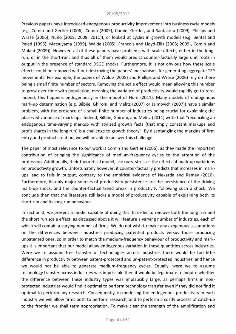
Figure 2: The cross correlation of US output and mark-ups, as a function of filter cut-off. (Dark gray is a significantly positive correlation (at 5%), light grey is a positive but insignificant one,
cross-hatched is a negative but insignificant one and white is a significantly negative one.)
Period length in years
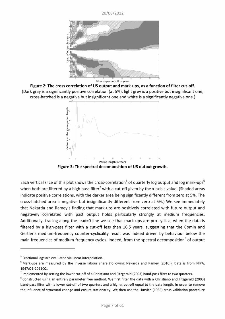
Figure 3: The spectral decomposition of US output growth.
Each vertical slice of this plot shows the cross-correlation5 of quarterly log output and log mark-ups6
when both are filtered by a high pass filter7 with a cut-off given by the x-axis’s value. (Shaded areas
indicate positive correlations, with the darker area being significantly different from zero at 5%. The
cross-hatched area is negative but insignificantly different from zero at 5%.) We see immediately
that Nekarda and Ramey’s finding that mark-ups are positively correlated with future output and
negatively correlated with past output holds particularly strongly at medium frequencies.
Additionally, tracing along the lead=0 line we see that mark-ups are pro-cyclical when the data is
filtered by a high-pass filter with a cut-off less than 16.5 years, suggesting that the Comin and
Gertler’s medium-frequency counter-cyclicality result was indeed driven by behaviour below the
main frequencies of medium-frequency cycles. Indeed, from the spectral decomposition8 of output
5 Fractional lags are evaluated via linear interpolation.
6 Mark-ups are measured by the inverse labour share (following Nekarda and Ramey (2010)). Data is from NIPA,
1947:Q1-2011Q2. 7 Implemented by setting the lower cut-off of a Christiano and Fitzgerald (2003) band-pass filter to two quarters.
8 Constructed using an entirely parameter free method. We first filter the data with a Christiano and Fitzgerald (2003)
band-pass filter with a lower cut-off of two quarters and a higher cut-off equal to the data length, in order to remove
the influence of structural change and ensure stationarity. We then use the Hurvich (1985) cross-validation procedure
2 4 6 8 10 12 14 16 18 20-5
-4
-3
-2
-1
0
1
2
3
4
5
2 4 6 8 10 12 14 16 18 200
1
2
3
4
5
6x 10
-5
Lead
of
ou
tpu
t in
yea
rs
Var
ian
ce a
t th
e gi
ven
per
iod
len
gth
20/08/2012
Page 8 of 61
growth shown in Figure 3, we see that mark-ups are significantly pro-cyclical when filtered at any
frequency corresponding to a peak in the spectral decomposition, including the medium-frequency
peak at twelve years. This establishes that the relevant medium-frequency cycles feature pro-
cyclical movements in mark-ups.
2.3. GDP variance
Our model predicts that the length of patent-protection should be positively correlated with the
observed size of medium-frequency cycles, at least for durations of patent-protection around those
we observe in reality. In Table 2 we exploit cross-country variation in effective patent duration to
demonstrate the presence of this correlation in the data, even when we control for GDP, legal
origins and various measures of political stability and risk. (Full details of the data are given in
footnotes to the table.) Patent duration in both 1960 and 2005 has a significantly positive effect (at
5%) on the strength of medium frequency cycles in all our five specifications, and only in in the
specification with no controls is there marginal evidence of misspecification (at 5%). Concerns
about endogeneity mean some restraint must be exerted in interpreting these results, but they are
nonetheless suggestive of a role for patent protection in the mechanism generating medium
frequency cycles in the data.
3. The model
Our base model is a standard quarterly real business cycle (RBC) model without capital, augmented
by the addition of models of endogenous competition, research, appropriation and invention. The
lack of capital means the underlying RBC model has no endogenous propagation mechanism,
making clearer the contribution of our additions.
Our model has a continuum of narrow industries, each of which contains finitely many firms
producing a unique product. The measure of industries is increased by the invention of new
products, which start their life patent-protected. However, we assume that product inventors lack
the necessary human capital to produce their product at scale themselves, and so they must license
out their patent to manufacturing firms. The duration of patent-protection is given by a geometric
distribution, in line with Serrano’s (2010) evidence on the large proportion of patents that are
allowed to expire early, perhaps because they are challenged in court or perhaps because another
new product is a close substitute. An earlier working-paper version of this model (Holden 2011)
considered the fixed duration case, which is somewhat less tractable. Allowing for a distribution of
protection lengths also allows us to give a broader interpretation to protection within our model.
Even in the absence of patent protection, the combination of contractual agreements such as
NDAs, and difficulties in reverse engineering, is likely to enable the inventor of a new product to
extract rents for a period.
to choose the bandwidth for the spectral-decomposition of the data, with his Stuetzle-derived estimator of the mean
integrated squared error, the standard Blackman-Tukey lag-weights estimate, and the Quadratic Spectral Kernel
recommended by Andrews (1991) amongst others.

20/08/2012
Page 9 of 61
Variable Spec. 1 Spec. 2 Spec. 3 Spec. 4 Spec. 5
Constant
-2.09811 (0.0300)
-2.14048 (0.0206)
-1.91285 (0.0180)
-2.70784 (0.0000)
-2.18372 (0.0009)
English legal origin9
-0.0506172 (0.8567)
-0.448554 (0.0810)
French legal origin9
-0.0557074 (0.8394)
-0.350747 (0.1653)
German legal
origin9
-0.151587 (0.6364)
-0.325196 (0.3154)
Log GDP per
effective adult10
0.0715242 (0.3620)
0.0707845 (0.3501)
GDP per effective adult growth10
7.39306 (0.1647)
7.24517 (0.1606)
Socioeconomic Conditions (ICRG)11
-0.224159 (0.0078)
-0.229358 (0.0044)
-0.170029 (0.0107)
Law and order (ICRG)11
-0.154013 (0.0856)
-0.150749 (0.0818)
-0.148729 (0.0856)
Logit overall
political risk (ICRG)11,12
0.806772 (0.0013)
0.811630 (0.0006)
0.823980 (0.0003)
Index of patent
duration, 196013
0.357215 (0.0336)
0.363052 (0.0242)
0.384211 (0.0131)
0.395486 (0.0044)
0.396382 (0.0060)
Index of patent duration, 200513
1.79391 (0.0223)
1.79854 (0.0197)
1.88715 (0.0140)
1.66419 (0.0053)
1.50279 (0.0133)
Observations 100 100 100 111 111
Specification
test p-values14
0.50, 0.31, 0.58
0.51, 0.20, 0.63
0.58, 0.08, 0.74
0.31, 0.06, 0.05
0.32, 0.12, 0.06
Table 2: The impact of patent duration on the strength of medium frequency cycles. Coefficients from assorted regression specifications. (P-values in brackets.) In all cases the
dependent variable is a logit transform of the proportion of GDP per effective adult growth variance that is at frequencies with periods greater than eight years15.
9 All countries which neither have English, French or German legal origins have Scandinavian legal origin in our sample.
Data is from La Porta, Lopez-de-Silanes and Shleifer (2008). 10
The intercept and the slope from running a regression of log GDP per effective adult on time. Data from the Penn
World Tables (Heston, Summers, and Aten 2011), samples identical to those used to construct the dependent variable. 11
International Country Risk Guide, The PRS Group. Data provided by the Nuffield College Data Library. Variables are
means of annual data from 1986-2007 (the largest span available for all countries in the sample). 12
This is the sum of the two components mentioned above, along with measures of government stability, the
investment profile, internal/external conflict, corruption, the military/religion in Politics, ethnic tensions, democratic
accountability and bureaucracy quality. The logit transform was taken after the mean. We ran regressions including all
components separately and our results were almost identical (p-values on patent duration of 0.0192 and 0.0172
respectively), but to save space here we focus on the components found to be most relevant. 13
Data kindly provided by Walter Park, updated from Ginarte and Park (1997). 14
Respectively, a normality test (Doornik and Henrik Hansen 2008), the White heteroskedasticity test (White 1980) and
the reset test with squares and cubes (Ramsey 1969). 15
Data is from the Penn World Tables (Heston, Summers, and Aten 2011) and spans 1950-2009, though many countries
have shorter samples. The shortest sample (of growth rates) is 23 years. We ran regressions including the sample length
as a regressor, but it consistently came out insignificant. Medium frequency variance shares are constructed from
spectral decompositions, following Levy and Dezhbakhsh (2003), where the spectral decomposition is performed using

20/08/2012
Page 10 of 61
Our model of endogenous competition within each industry is derived from Jaimovich (2007). We
chose the Jaimovich model as it is a small departure from the standard Dixit-Stiglitz (1977) set-up,
and leads to some particularly neat expressions. Similar results could be attained with Cournot
competition, or the Translog form advocated by Bilbiie, Ghironi, and Melitz (2008). One important
departure from the Jaimovich model is that in our model entry decisions take place one period in
advance. This is natural as we wish to model research as taking place after entry but before
production.
Productivity within a firm is increased by performing research or appropriation. We regard process
research as incremental, with regular small changes rather than the unpredictable jumps found in
Schumpetarian models (Aghion and Howitt 1992; Wälde 2005; Phillips and Wrase 2006).
Throughout, we assume that only products are patentable,16 and so by exerting effort firms are
able to “appropriate” process innovations from other industries to aid in the production of their
own product. This appropriation is costly since technologies for producing other products will not
be directly applicable to producing a firm’s own product. We assume that technology transfer
within an industry is costless however, due to intra-industry labour flows and the fact that all firms
in an industry are producing the same product. This is important for preserving the tractability of
the model, as it means that without loss of generality we may think of all firms as just existing for
two periods, in the first of which they enter and perform research, and in the second of which they
produce.
The broad timing of our model is as follows. At the beginning of period invention takes place,
creating new industries. All holders of current patents (including these new inventors) then decide
what level of license fee to charge. Then, based on these license fees and the level of overhead
costs, firms choose whether to enter each industry. Next, firms perform appropriation, raising their
next-period productivity towards that of the frontier, then research, further improving their
productivity next period. In period they then produce using their newly improved production
process. Meanwhile, a new batch of firms will be starting this cycle again.
We now give the detailed structure of the model.
the parameter free method outlined in footnote 8, with the initial filter set to accept period lengths between 2 and 59
years (the length of the largest samples). 16
This is at least broadly in line with the law in most developed countries: ideas that are not embedded in a product (in
which category we include machines) generally have at most limited patentability. In the U.S., the most recent Supreme
court decision found that the following was “a useful and important clue” to the patentability of processes (Bilski v.
Kappos, 561 U.S. ___ (2010)): “a method claim is surely patentable subject matter if (1) it is tied to a particular machine
or apparatus, or (2) it transforms a particular article into a different state or thing” (In re Bilski, 545 F.3d 943, 88
U.S.P.Q.2d 1385 (Fed. Cir. 2008)). This “machine or transformation” test was widely believed at the time to have ended
the patentability of business processes (The Associated Press 2008), and this position was only slightly softened by Bilski
v. Kappos.

20/08/2012
Page 11 of 61
3.1. Households
There is a unit mass of households, each of which contains members in period . The
representative household maximises:
∑ [
(
)
]
where is aggregate period consumption, is aggregate period labour supply, is a demand
shock, is a labour supply shock, is the discount rate and is the inverse of the Frisch elasticity
of labour supply to wages, subject to the aggregate budget constraint that
, where is the aggregate number of (zero net supply) bonds bought by households
in period , is the period wage, is the period sale price of a (unit cost) bond bought in
period , and is the households’ period dividend income. In the following, where we refer
to preference shocks we mean either a shock to or a shock to . However, both of these shocks
may be interpreted as proxying for real changes in the economy that are independent of
preferences. For example, will capture changes in government consumption demand coming
from wars, and will pick up changes in marginal tax rates and in the degree of imperfect
competition in labour markets.
Let be the households’ period stochastic discount factor, then the households’ first order
conditions imply:
[ ]
3.2. Aggregators
The consumption good is produced by a perfectly competitive industry from the aggregated output
( ) of each industry [ ], using the following Dixit-Stiglitz-Ethier (Dixit and Stiglitz 1977;
Ethier 1982) style technology:
[∫ ( )
]
where
is the elasticity of substitution between goods and where the exponent on the measure
of industries ( )17 has been chosen to remove the preference for variety in consumption.18
17 The subscript here reflects the fact that industries are invented one period before their product is available to
consumers. 18
Incorporating a preference for variety would not change the long-run stability of our model.

20/08/2012
Page 12 of 61
Normalising the price of the aggregate consumption good to , and writing ( ) for the price of the
aggregate good from industry in period , we have that:
( )
( )
[
∫ ( )
]
Similarly, each industry aggregate good ( ) is produced by a perfectly competitive industry from
the intermediate goods ( ) for { ( )},19 using the technology:
( ) ( ) [ ∑ ( )
( )
]
where ( ) controls the degree of differentiation between firms, relative to that between
industries.
This means that if ( ) is the price of intermediate good in industry :
( ) ( )
( )( ( )
( ))
( ) [
( )∑ ( )
( )
]
3.3. Intermediate firms
3.3.1. Pricing
Firm in industry has access to the linear production technology ( ) ( ) ( ) for
production in period . As in Jaimovich (2007), strategic profit maximisation then implies that in a
symmetric equilibrium ( ) ( ) ( ( ))
( ) ( ( ))
( ), where:
( ) ( )
( ) ( ) ( ]
is the industry mark-up in period and ( ) ( ) is the productivity shared by all firms
in industry in symmetric equilibrium.
19 Again, the subscript reflects the fact that firms enter one period before production.

20/08/2012
Page 13 of 61
From aggregating across industries we have that
where:
[
∫ [
( )]
]
determines the aggregate mark-up and where:
[
∫ [
( )
( )]
]
[
∫ [
( )]
]
is a measure of the aggregate productivity level.20
3.3.2. Sunk costs: rents, appropriation and research
Following Jaimovich (2007) we assume that the number of firms in an industry is pinned down by
the zero profit condition that equates pre-production costs to production period revenues. Firms
borrow in order to cover these upfront costs, which come from four sources.
Firstly, firms must pay a fixed operating cost that covers things such as bureaucracy, human
resources, facility maintenance, training, advertising, shop set-up and capital installation/creation.
Asymptotically, the level of fixed costs will not matter, but including it here will help in our
explanation of the importance of patent protection for long run growth.
Secondly, if the product produced by industry is currently patent-protected, then firms must pay a
rent of ( ) units of the consumption good to the patent-holder for the right to produce in their
industry. Since all other sunk costs are paid to labour, for convenience we define ( )
( )
, i.e.
the labour amount equivalent in cost to the rent.
Thirdly, firms will expand labour effort on appropriating the previous process innovations of the
leading industry. We define the level of the leading technology within industry by ( )
{ ( )} ( ) and the level of the best technology anywhere by [ ]
( ).
Due to free in-industry transfer, even without exerting any appropriation effort, firms in industry
may start their research from ( ) in period . By employing appropriation workers a firm may
raise this level towards .
20 Due to the non-linear aggregation, it will not generically be the case that aggregate output is aggregate labour input
times . However, the aggregation chosen here is the unique one under which aggregate mark-ups are known one
period in advance, as industry mark-ups are.

20/08/2012
Page 14 of 61
We write ( ) for the base from which firm { ( )} will start research in period , and
we assume that if firm employs ( ) units of appropriation labour in period then:
( ) [
( ) (
( ) ) ( )
( )
( )
( )]
(3.1)
where is the productivity of appropriation labour, controls the extent to which
appropriation is getting harder over time (due, for example, to the increased complexity of later
technologies) and where controls whether the catch-up amount is a proportion of the
technology difference in levels ( ), log-levels ( ) or anything in between or beyond. This
specification captures the key idea that the further a firm is behind the frontier, the more
productive will be appropriation. Allowing for appropriation (and research, and invention) to get
harder over time is both realistic, and essential for the tractability of our model, since it will lead
our model to have a finite dimensional state vector asymptotically, despite all the heterogeneity
across industries.
Fourthly and finally, firms will employ labour in research. If firm { ( )} employs ( )
units of research labour in period , its productivity level in period will be given by:
( ) ( ) ( ( )
( )
( ))
where is the productivity of research labour, controls the extent to which research is
getting harder over time, ( ) is a shock representing the luck component of research,
and controls the “parallelizability” of research. 21 If , research may be perfectly
parallelized so arbitrarily large quantities may be performed within a given period without loss of
productivity, but if is large, then the productivity of research declines sharply as the firm attempts
to pack more into one period. The restriction that means that the difficulty of research is
increasing over time faster than the difficulty of appropriation. This is made because research is
very much specific to the industry in which it is being conducted, whereas appropriation is a similar
task across all industries attempting to appropriate the same technology, and hence is more likely
to have been standardised, or to benefit from other positive spillovers.
In the following, we will assume that ( ) so that all firms in all industries receive the same
“idea” shock. We make this assumption chiefly for simplicity, but it may be justified by appeal to
common inputs to private research, such as university research output or the availability of new
tools, or by appeal to in-period labour market movements carrying ideas with them. We will see in
the following that allowing for industry-specific shocks has minimal impact on our results, providing
there are at least correlations across industries (plausible if they are producing similar products).
For concreteness, we assume that ( ), where and ( ).
21 Peretto (1999) also looks at research that drives incremental improvements in productivity, and chooses a similar
specification. The particular one used here is inspired by Groth, Koch, and Steger (2009).

20/08/2012
Page 15 of 61
3.3.3. Research and appropriation effort decisions
Firms are owned by households and so they choose research and appropriation to maximize:
[ ( ( )
( )) ( )] [
( ) ( )
( ) ]
It may be shown that, for firms in frontier industries (those for which ( )
), if an equilibrium
exists then it is unique and symmetric within an industry; but we cannot rule out the possibility of
asymmetric equilibria more generally. 22 However, since the coordination requirements of
asymmetric equilibria render them somewhat implausible, we restrict ourselves to the unique
equilibrium in which all firms within an industry choose the same levels of research and
appropriation. Let us then define effective research performed by firms in industry by ( )
( )
( ) (valid for any { ( )}) and effective appropriation performed by firms
in that industry by ( )
( )
( ) (again, valid for any { ( )}).
Providing
( ) { } , and (for the second order conditions 23 and for
uniqueness), combining the first order and free entry conditions then gives us that, in the limit as
: 24
( ) {
( ) ( )
(
( ) ( )
) ( )
( ) ( )} (3.2)
and: ( ) { ( ) √ { ( ) ( )}} (3.3)
22 The equilibrium concept we use is that of pure-strategy subgame-perfect local Nash equilibria (SPLNE) (i.e. only
profitable local deviations are ruled out). We have no reason to believe the equilibrium we find is not in fact a
subgame-perfect Nash equilibria (SPNE). Indeed, if there is a pure-strategy symmetric SPNE then it will be identical to
the unique pure-strategy symmetric SPLNE that we find. Furthermore, our numerical investigations suggest that at least
in steady-state, at our calibrated parameters, the equilibrium we describe is indeed an SPNE. (Code available on
request.) However, due to the analytic intractability of the second stage pricing game when productivities are
asymmetric, we cannot guarantee that it remains an equilibrium away from the steady-state, or for other possible
calibrations. However, SPLNE’s are independently plausible since they only require firms to know the demand curve
they face in the local vicinity of an equilibrium, which reduces the riskiness of the experimentation they must perform
to find this demand curve (Bonanno 1988). It is arguable that the coordination required to sustain asymmetric equilibria
and the computational demands of mixed strategy equilibria render either of these less plausible than our SPLNE. 23
The second order condition for research may be derived most readily by noting that when ( ) , (i.e. ( ) )
the first order condition for research is identical to the one that would have been derived had there been a continuum
of firms in each industry with exogenous elasticity of substitution ( )
( ). That it holds more generally follows by
continuity. Since ( ) is bounded above, no matter how much appropriation is performed the highest solution of
the appropriation first order condition must be at least a local maximum. 24
The first order and zero profit conditions are reported in an appendix, section 8.1, where we also derive these
solutions. We do not assume when simulating, but it leads here to expressions that are easier to interpret.

20/08/2012
Page 16 of 61
where ( ) ( )25 is small when firm behaviour is highly distorted by firms’ incentives to
deviate from choosing the same price as the other firms in their industry, off the equilibrium path
(so ( ) as ( ) ), and ( ) and ( ) are increasing in an industry’s distance from the
frontier,26 as the further behind a firm is, the greater are the returns to appropriation.
Equations (3.2) and (3.3) mean that research and appropriation levels are increasing in the other
sunk costs a firm must pay prior to production but decreasing in mark-ups. They also mean that the
strategic distortions caused by there being a small number of firms within an industry tend to
reduce research and appropriation levels. Other sunk costs matter for research levels because
when other sunk costs are high, entry into the industry is lower, meaning that each firm receives a
greater slice of production-period profits, and so has correspondingly amplified research incentives.
Why mark-up increases decrease research incentives is clearest when those mark-up increases are
driven by exogenous decreases in the elasticity of substitution. When products are close substitutes
then by performing research (and cutting its price) a firm may significantly expand its market-share,
something that will not happen when the firm’s good is a poor substitute for its rivals. When
( ) (i.e. there are a lot of firms in the industry) firms act as if they faced an exogenous
elasticity of substitution ( )
( ), and so when mark-ups are high they will want to perform little
research. When ( ) is small (i.e. there are only a few firms) then firms behaviour is distorted by
strategic considerations. Each firm realises that if they perform extra research today then their
competitors will accept lower mark-ups the next period. This reduces the extent to which research
allows market-share expansion, depressing research incentives.
Perhaps counter-intuitively, the minimum value of ( ) occurs when there is a strictly positive
number of firms in the industry. It is certainly true that if there is a single firm in an industry, then,
as you would expect, very little research will be performed (because the firm’s only incentive to cut
prices comes from competition from other industries, competition which is very weak, since those
industries are producing poor substitutes to its own good). However, this drop in research
incentives is working entirely through the mark-up channel, and so in fact we also have that
( ) as ( ) . One intuition for this is that there can be no strategic behaviour when there
is only a single firm.
The key thing to note about (3.2) and (3.3) is that research and appropriation are independent of
the level of demand, except insomuch as demand affects mark-ups and the level of the strategic
distortion. This is because when demand is high there is greater entry, so each firm still faces
roughly the same demand. This is essential for removing the short-run scale effect.
In industries that are no longer patent-protected, rents will be zero (i.e. ( ) ). Since research
is getting harder at a faster rate than appropriation ( ), at least asymptotically, no research
25 Defined in the appendix, section 8.1.
26 ( )
[
( )
( )
( ) ( )
( )
] [ ( ( )
)
] , ( ) ( )
( )
( ) ( )
( )
( )
[
( ) ( ) ] [
( ( )
)
] ( ( )
)
.

20/08/2012
Page 17 of 61
will be performed in these industries. This is because ( )
[
( ) ] ( ) is
asymptotically negative since ( ) ( ]. For growth to continue forever in the absence of
patent protection, we would require that the overhead cost ( ) was growing over time at exactly
the right rate to offset the increasing difficulty of research. This does not seem particularly
plausible. However, it will turn out that optimal patent rents grow at exactly this rate, so with
patent protection we will be able to sustain long run growth even when overhead costs are
asymptotically dominated by the costs of research. In the presence of sufficiently-severe financial
frictions of the “pledgibility constraint” form (Hart and Moore 1994), it may be shown that long run
growth is sustainable even without patent protection. We leave the details of this for future work.
Appropriation is performed in an industry if and only if ( ) , which, for a non-patent
protected industry no longer performing research, is true if and only if:
( )
(
( )
( )
( )
( )
)
The left hand side of this equation is the relative productivity of the industry compared to the
frontier. The right hand side of this equation will be shrinking over time at roughly
times the
growth rate of the frontier, meaning the no-appropriation cut-off point is also declining over time.
Indeed, we show in an appendix, section 8.2, that asymptotically the relative productivity of non-
protected firms shrinks at
[
]
times the growth rate of the frontier. This is plausible since
productivity differences across industries have been steadily increasing over time,27 and is
important for the tractability of our model since it enables us to focus on the asymptotic case in
which non-protected firms never perform appropriation.
3.4. Inventors
Each new industry is controlled by an inventor who owns the patent rights to the product the
industry produces. Until the inventor’s product goes on sale, the patent holder can successfully
protect their revenue stream through contractual arrangements, such as non-disclosure
agreements. This means that even in the absence of patent-protection a patent holder will receive
one period of revenues. In this period, and each subsequent one for which they have a patent, the
inventor optimally chooses the rent ( ) (or equivalently ( )) to charge all the firms that wish to
produce their product. We are supposing inventors lack the necessary human capital to produce
their product at scale themselves.
27 Some indirect evidence for this is provided by the increase in wage inequality, documented in e.g. Autor, Katz, and
Kearney (2008). Further evidence is provided by the much higher productivity growth rates experienced in
manufacturing, compared to those in services (mostly unpatented and unpatentable), documented in e.g. Duarte and
Restuccia (2009).

20/08/2012
Page 18 of 61
The inventor of a new product has a probability of of being granted a patent to enable them
to extract rents for a second period. After this, if they have a patent at , then they face a constant
probability of of having a patent at .
The reader should have a firm such as Apple in mind when thinking about these inventors. Apple
has no manufacturing plants and instead maintains its profits by product innovation and tough
bargaining with suppliers.
3.4.1. Optimal rent decisions
Inventor’s businesses are also owned by households; hence, an inventor’s problem is to choose
( ) for to maximise their expected profits, which are given by:
∑ ( ) [∏
] ( ) ( )
subject to an enforceability constraint on rents. If the rents charged by a patent-holder go too high,
a firm is likely to ignore them completely in the hope that either they will be lucky, and escape
having their profits confiscated from them by the courts (since proving patent infringement is often
difficult), or that the courts will award damages less than the licence fee. This is plausible since the
relevant U.S. statute states that “upon finding for the claimant the court shall award the claimant
damages adequate to compensate for the infringement but in no event less than a reasonable
royalty for the use made of the invention by the infringer, together with interest and costs as fixed
by the court”. 28,29 The established legal definition of a “reasonable royalty” is set at the outcome of
a hypothetical bargaining process that took place immediately before production,30 so patent-
holders may just as well undertake precisely this bargaining process before production begins.31
28 35 U.S.C. § 284 Damages.
29 The reasonable royalty condition is indeed the relevant one for us since our assumption that the patent-holder lacks
the necessary human capital to produce at scale themself means it would be legally debatable if they had truly “lost
profits” following an infringement (Pincus 1991). 30
Georgia-Pacific, 318 F. Supp. at 1120 (S.D.N.Y. 1970), modified on other grounds, 446 F.2d 295 (2d Cir.), cert. denied,
404 U.S. 870 (1971), cited in Pincus (1991), defines a reasonable royalty as “the amount that a licensor (such as the
patentee) and a licensee (such as the infringer) would have agreed upon (at the time the infringement began) if both
had been reasonably and voluntarily trying to reach an agreement; that is, the amount which a prudent licensee—who
desired, as a business proposition, to obtain the license to manufacture and sell a particular article embodying the
patented invention—would have been willing to pay as a royalty and yet be able to make a reasonable profit and which
amount would have been acceptable by a prudent patentee who was willing to grant a license.” 31
In any case, if we allow for idiosyncratic “idea shocks” firms will wish to delay bargaining until this point anyway, since
with a bad shock they will be less inclined to accept high rents. Patent-holders also wish to delay till this point because
the more sunk costs the firms have already expended before bargaining begins, the greater the size of the “pie” they
are bargaining over.

20/08/2012
Page 19 of 61
This leads patent-holders to set:
( )
[ ( )
( ) ] (3.4)
at least for sufficiently large , where ( ) is the bargaining power of the firm, in the sense of
the generalized Nash bargaining solution. The simple form of this expression comes from the fact
that a firm’s production period revenues (which is what is being bargained over) are precisely equal
to the costs they face prior to production, thanks to the free entry condition. A full description of
the legally motivated bargaining process is contained in an appendix, section 8.3, along with a
discussion of some technical complications pertaining to off equilibrium play.
From combining (3.2) and (3.4) then, at least for sufficiently large , in the limit as as , we
have that:
( )
( ) ( ) ( )
(
( ) )
( ) ( )
For there to be growth in the long run then, we require ( ) ( ), which together with the
second order and appropriation uniqueness conditions means that it must at least be true that
( ) { }.32 We see that, once optimal rents are allowed for, research is no longer
decreasing in mark-ups within an industry, at least for firms at the frontier. Mathematically, this is
because the patent-holder sets rents as such a steeply increasing function of research levels. More
intuitively, you may think of the patent-holder as effectively controlling how much research is
performed by firms in their industry, and as taking most of the rewards from this research. It is then
unsurprising that we reach these Schumpeterian conclusions.
The empirical evidence (Scott 1984; Richard C. Levin, Cohen, and Mowery 1985; Aghion et al. 2005;
Tingvall and Poldahl 2006) suggests that the cross-industry relationship between competition and
research takes the form of an inverted-U. Based on the fact that strategic distortions are maximised
(i.e. ( ) is minimised) when there is a small finite number of firms, one might perhaps hope that
this holds in our model too. Unfortunately, the maximum of ( )
( ) (and hence of research) as a
function of ( ) may be shown to always occur at some ( ) . While fractional entry may be a
legitimate way of modelling niche products that are never fully commercialised, we prefer to
explain the inverted-U in the data with reference to the cross-sectional distribution of industries.
New industries will start with a production process behind that of the frontier, and thus firms in
them will wish to perform large amounts of appropriation and relatively small amounts of research,
since appropriation is a cheaper means of increasing productivity for a firm behind the frontier. In
the presence of a luck component to appropriation (not included above, for simplicity) this leads
new industries to have the highest degree of productivity dispersion, as older industries remain
32 If the number of firms in protected industries is growing over time then ( ) , so asymptotically these conditions
are equivalent.

20/08/2012
Page 20 of 61
close to the frontier. As a result of this high productivity dispersion, there will be firms in new
industries setting both very high, and very low mark-ups, which, combined with the fact they are
performing less research than more mature patent-protected industries, would generate an
inverted-U.
3.4.2. Invention and long-run stability
We consider invention as a costly process undertaken by inventors until the expected profits from
inventing a new product fall to zero. New products appear at the end of the product spectrum.
Additionally, once a product has been invented, it cannot be “uninvented”. Therefore, the product
index always refers to the same product, once it has been invented.
There is, however, no reason to think that newly invented products will start off with a competitive
production process. A newly invented product may be thought of as akin to a prototype: yes,
identical prototypes could be produced by the same method, but doing this is highly unlikely to be
commercially viable. Instead, there will be rapid investment in improving the product’s production
process until it may be produced as efficiently as its rivals can be. In our model, this investment in
the production process is performed not by the inventor but by the manufacturers. Prototyping
technology has certainly improved over time;33 in light of this, we assume that a new product is
invented with a production process of level ( )
, where ( ) controls initial relative
productivity.
Just as we expect process research to be getting harder over time, as all the obvious process
innovations have already been discovered, so too we may expect product invention to be getting
harder over time, as all the obvious products have already been invented. In addition, the necessity
of actually finding a way to produce a prototype will result in the cost of product invention also
being increasing in ( ), the initial productivity level of the process for producing the new product.
As a result of these considerations, we assume that the labour cost is given by ( )
, where
determines the difficulty of invention and where and control the rate at which
inventing a new product gets more difficult because of, respectively, an increased number of
existing products or an increased level of productivity.
We are assuming there is free entry of new inventions, so the marginal entrant must not make a
positive profit from entering. That is, must be as small as possible such that:
( )
∑ ( ) [∏
] ( ) ( )
If, after a shock, invention can satisfy this equation with equality without the growth rate of the
stock of products turning negative, then the measure of firms will not have to adjust significantly.
33 Examples of recent technologies that have raised the efficiency of prototype production include 3D printing and
computer scripting languages such as Python.

20/08/2012
Page 21 of 61
However, if the constraint binds, then the measure of firms will have to adjust instead,
meaning there may be an asymmetry in the response of mark-ups to certain shocks.
It may be shown that, in the long run,
( ) (where is the asymptotic growth
rate of the variable ). Therefore, if the stock of products will grow at exactly the same
rate as population, and away from this special case it will be growing more slowly. If invention were
to stop asymptotically, eventually there would be no protected industries, and hence no
productivity growth. Therefore, for long-run growth, we either require that (which will
hold providing research is getting more difficult sufficiently slowly, as long as population growth
continues), or that there is sufficiently fast depreciation of the stock of products.34 Even without
product depreciation, productivity growth may be sustained indefinitely in the presence of a
declining population if the government offers infinitely renewable patent-protection.
The existence of a solution for our model at all time periods requires the number of firms in a
protected industry to be bounded below asymptotically. The previous result on the growth rate of
the stock of products implies it is sufficient that (
)
for this to hold. This
inequality is guaranteed to be satisfied providing
is sufficiently small. To do this while also
ensuring that requires that {
( )}
, which will hold for a positive
measure of parameter values providing population growth is strictly positive.35
Assuming this condition holds, we may show36 that providing the growth rate of the productivity of
newly invented products is sufficiently close to the frontier growth rate (i.e. does not decline too
quickly37), asymptotically catch-up to the frontier is instantaneous in protected industries, and the
frontier growth rate is stationary. This instantaneous catch-up to the frontier means that, had we
allowed for industry-specific shocks, all other protected industries would “inherit” the best industry
shock, the period after it arrived. This justifies our focus on aggregate “idea” shocks. Additionally,
instantaneous catch-up to the frontier means that providing there is population growth or product
depreciation, long-run growth may be sustained even in the absence of patent-protection (i.e.
34 Bilbiie, Ghironi, and Melitz (2007) include such product depreciation in their model. We have chosen not to model it
here. 35
More generally, when population is stable, providing there is sufficiently fast (proportional) depreciation of the stock
of products, we just require that
.
36 Suppose ( )
is a sequence of industries, all protected at , whose productivity grows at rate
asymptotically. We conjecture that ( )
( ) and verify.
This assumption implies that effective
research is asymptotically bounded, since mark-ups are. Hence from (3.3), since , effective appropriation is
growing at a rate in the interval (
) ( ). Therefore
( )
( ) is growing at a rate in the
interval (
). For our claim to be verified we then just need that
, which certainly holds when as .
37 As it is sufficient that is declining at less than half the rate that
is growing.

20/08/2012
Page 22 of 61
when ), as the one period in which the inventor has a first mover advantage is sufficient for
their industry to surpass the existing frontier.
If the number of firms in protected industries were asymptotically infinite, then our simulations
would tell us nothing about the consequences of the variations in this number that we might see
non-asymptotically. Therefore, it will be helpful if it is additionally the case that the number of firms
is asymptotically finite. To guarantee this will, unfortunately, require a knife-edge assumption,
namely that (
)
. To satisfy this without restricting population growth rates
means (so invention is not made more difficult by the number of existing products) and
(so prototype production is increasing in difficulty at the same rate as research). The former
assumption may be justified by noting that many situations in which invention is apparently getting
harder over time because of congestion effects may equally well by explained by production-
process-difficulty effects. The latter assumption is immediately plausible, since both parameters are
measuring the complexity of working with a given production process. However, unlike with knife-
edge growth models whereby relatively slight departures from the stable parameter values results
in growth that could not possibly explain our observed stable exponential growth, here, away from
the knife-edge case we will have slowly decreasing mark-ups, consistent with Ellis’s (2006) evidence
of a persistent decline in UK whole economy mark-ups over the last thirty years and Kim’s (2010)
evidence of non-stationarity in mark-ups.
We assume then that . Since asymptotically non-protected industries
perform no research or appropriation under these assumptions, their entry cost to post-entry
industry profits ratio is tending to zero, meaning their number of firms will tend to infinity as
. This is in line with our motivating intuition that excess entry in non-protected industries kills
research and appropriation incentives.
4. Simulations
With , as the behaviour our model tends towards stationarity in the
key variables. It is this asymptotically stationary model that we simulate. For convenience we define
. The full set of equations of the de-trended model are given in an appendix, section
8.4. The definition of equilibrium here is entirely standard.
When , it may be shown analytically that the equations determining the model’s
steady-state have at most two solutions with more than one firm in each industry. However, only
one of these two solutions exists for large values of , i.e. when invention is costly. Since we think
that in reality invention is getting harder over time due to congestion effects (i.e. ), any
solution that only exists for small values of is non-feasible. Our numerical investigations suggest
that the model always has at most these two equilibria, and that always at most one of them exists

20/08/2012
Page 23 of 61
for large values of .38 However, since the existence of multiple-equilibria is indicative that linear
approximations may be inaccurate in that region, rather than just picking the solution that exists for
arbitrarily large , we instead restrict the parameter space to regions in which there is a unique
solution. This ensures that the value of we use is indeed large, in this sense.
Since always occurs as a group, without loss of generality we may make the normalization
. We fix all of the model’s other parameters, except , to the values estimated for our
extended model in section 5. is set such that the number of firms in patent-protected industries
in this model is equal to that of the estimated extended model. The full parameterisation is
reported in an appendix (section 8.7). At the chosen parameters, the model has a unique solution,
which will exist for arbitrarily high values of .
4.1. Simulation method
We take a first-order perturbation approximation around the non-stochastic steady state,
perturbing in the variance of shocks, and solve for the rational expectations solution of the
linearized model.39 As we have previously mentioned, the zero lower bound on net product
creation (i.e. on ) means there may be an asymmetric response to sufficiently large shocks, but
in fact we do not find that the bound is hit with shocks of plausible magnitudes.
4.2. Impulse responses
In Figure 4 we present the impulse responses that result from one per cent IID (hence non-
persistent) shocks to “ideas” ( ), labour supply ( ), demand ( ) and population growth ( ).
Each graph is given in terms of per cent deviations from the value the variable would have taken
had the shock never arrived, and the horizontal axis shows time in years, though this remains a
quarterly model. Each shock is in a different column, and the key response variables are in rows.
The principle mechanism of our paper is shown most clearly by the population growth rate shock,
shown in the final column. (We do not wish to advance population shocks as a key driver of
business cycles though, since real rigidities will significantly reduce their impact.) Following a
permanent increase in population, demand is permanently higher, so, in the long run, the number
of industries must grow to balance this out. Given sufficiently inelastic labour supply, this long-run
increase in the measure of industries requires a short-run substitution of labour from production to
invention, pushing down consumption and pushing up wages, and so moderating the rate at which
invention will grow. Consequently, in the short run some of the additional demand is absorbed by
fluctuations in the number of firms in each industry. Without this additional margin of adjustment,
this shock would have led to a large increase in average firm sizes, with a consequent increase in
the frontier growth rate and counter-factually large unit root in output.
38 It may be shown analytically that the complete model may always be solved by solving a single nonlinear equation,
which was always concave for all the parameters we examined. 39
This was performed using Dynare (Adjemian et al. 2011).

20/08/2012
Page 24 of 61
Despite the tiny movement in frontier productivity (less than ), there is still however a
substantial movement in aggregate productivity in the medium-term. Following the shock, more
new products are being invented each period, meaning that a greater proportion of industries are
relatively new, and so a greater proportion are patent-protected. But because patent-protected
industries have such strong incentives to catch-up to the frontier, patent-protected industries are
more productive than non-protected ones, so an increase in the proportion of industries that are
patent protected means an increase in aggregate productivity. Patent-protected industries also
have higher mark-ups due to the cost of paying license fees, and so we also see a rise in mark-ups
over the medium-term. It is this mechanism that generates medium-frequency pro-cyclical mark-
ups in our model.40
This mechanism also underlies our model’s response to the other shocks we consider. Following a
positive labour supply shock invention is temporarily cheaper, meaning more new industries and
consequently higher productivity and mark-ups.41 Following a demand shock labour is transferred
away from research and invention towards production, in order to satisfy the temporary higher
demand. This drop in invention on impact means that demand shocks actually reduce output in
subsequent periods. This is no longer the case when the shock has some persistence, or when there
are real rigidities.
An idea shock permanently increases the productivity of patent-protected industries. Over time,
these industries fall out of patent-protection, carrying their higher productivity with them, and thus
increasing the average productivity of non-protected firms too. Consequently, aggregate
productivity slowly rises towards its permanently higher long run level. However, since the
magnitude of the original shock was very small, this will not result in a large unit root in output.
Following the shock, patent-protected industries are relatively more productive than normal, and
so they are also relatively more profitable. This means patent holders can extract higher rents, and
so we see an increase in invention with a corresponding increase in mark-ups over the medium-
term.
40 Pavlov and Weder (2012) also develop a business cycle model capable of generating pro-cyclical mark-ups, via the
changing importance of different types of buyers over the business cycle. The properties of these buyers are exogenous
in their model however, whereas the properties of the different types of sellers that drive our results are endogenous. 41
Were the number of firms per protected industry to absorb the cost-cut instead, then next-period mark-ups would
fall and so future wages would rise. However, an expected increase in wages will increase invention today, since
inventor returns are increasing in the expected future wage. Hence, invention must rise in the period of the shock.

20/08/2012
Page 25 of 61
Positive idea shock ( ) Negative labour supply shock ( )
Positive demand shock ( ) Population shock ( )
Figure 4: Impulse responses from the core model.
(Vertical axes are in percent, horizontal axes are in years.)
5. Extended model and empirical tests
In order to compare our model to the data seriously, we incorporate habits, capital, and imperfect
competition in labour markets. We allow for the possibility of stochastic movements in the key
parameters , and ,42 (though it turns out that the data favours constant values for these
42 These parameters are assumed to be known before the entry decision at , for production in period .
0 10 20 300
2
4x 10
-3
0 10 20 30-1
-0.5
0x 10
-4
0 10 20 30-2
-1
0x 10
-3
0 10 20 30-4
-2
0x 10
-3
0 10 20 300
2
4x 10
-3
0 10 20 30-2
0
2x 10
-3
0 10 20 30-0.05
0
0.05
0 10 20 300
0.2
0.4
0 10 20 300
2
4x 10
-3
0 10 20 30-0.01
0
0.01
0 10 20 30-0.2
0
0.2
0 10 20 300
0.2
0.4
0 10 20 30-5
0
5x 10
-5
0 10 20 30-0.05
0
0.05
0 10 20 30-0.05
0
0.05
0 10 20 30-0.01
0
0.01
0 10 20 30-5
0
5x 10
-3
0 10 20 30-0.02
0
0.02
0 10 20 30-1
0
1
0 10 20 30-0.5
0
0.5
0 10 20 30-2
0
2x 10
-4
0 10 20 30-2
0
2x 10
-3
0 10 20 30-0.05
0
0.05
0 10 20 30-0.05
0
0.05
0 10 20 30-5
0
5x 10
-3
0 10 20 30-0.05
0
0.05
0 10 20 30-1
0
1
0 10 20 30-1
0
1
0 10 20 300
1
2x 10
-3
0 10 20 30-0.01
-0.005
0
0 10 20 30-0.4
-0.2
0
0 10 20 300
0.5
1
0 10 20 30-0.02
0
0.02
0 10 20 30-0.1
0
0.1
0 10 20 30-2
0
2
0 10 20 300
2
4
0 10 20 30-0.1
0
0.1
0 10 20 30-5
0
5
0 10 20 30-50
0
50
0 10 20 30-20
0
20
Productivity of protected
industries (𝐴𝑡 )
Productivity of non-protected industries (𝐴𝑡
)
Aggregate productivity
(𝐴𝑡)
Labour supply per capita
(𝐿𝑡 𝑁𝑡 )
Output (=cons.) per
capita (𝑌𝑡 𝑁𝑡 )
Aggregate mark-ups
(𝜇𝑡)
Num. firms in protected.
industries (𝐽𝑡 )
Number of industries (𝐼𝑡)
Proportion of protected
industries (𝓈𝑡)
R&D expenditure over output

20/08/2012
Page 26 of 61
parameters), and we specify an ( ) form for these and all other shocks, with the exception of ,
the true technology shock which remains uncorrelated across time. The data will be allowed to
choose which, if any, of these shocks might be important drivers of business cycles, at high, or
medium frequencies.
Additionally, we include intermediate goods as a factor of production, which is necessary in order
to reconcile the low mark-ups found in micro-evidence with the higher mark-ups implied by the
inverse labour share. The presence of intermediates in production will amplify shocks in our
economy, as it implies that an increase in the proportion of industries that are patent-protected
means intermediate inputs are cheaper for non-protected industries, increasing their output too.
To potentially dampen our model’s overly powerful amplification mechanism, we include some
spill-overs from frontier productivity growth; these mean that the variance of TFP may be less than
that of .
We also allow for sticky nominal wages in line with the micro-evidence of Barattieri, Basu, and
Gottschalk (2010), and to enable us to make preliminary remarks about the possible medium-term
impact of monetary policy. In all of the impulse responses presented below though, we will show
the model’s performance both with and without this feature. We do not include sticky prices for
several reasons. Firstly, it is hard to reconcile the highly sophisticated behaviour of firms in our
model with the naïve behaviour of firms in the Calvo (1983) model. Secondly, introducing sticky
prices would make solving for firm behaviour very complicated, unless the sticky prices were only
introduced to a separate retail sector, further increasing the size of our model. Finally, as is well
known, introducing sticky prices results in counter-cyclical mark-ups, contrary to the evidence of
Nekarda and Ramey (2010). The observed frequency of price adjustment can perhaps be reconciled
with pro-cyclical mark-ups using a consumer search model as in Head et al. (2011). We do not
pursue this avenue here.
5.1. Model changes
We assume that firm in industry has access to the production technology:
( ) ( ) ( ) [
( ) ( ) ]
where ( ) is their level of intermediate good input and
( ) is the quantity of capital they
hire from households, at a cost of per unit. We use a Hicks-neutral specification here since it
minimises the changes necessary to the model without capital. (In particular, profits take the same
form, and so research incentives are identical.)
Research, appropriation and invention will also use capital, but we assume that the capital they use
is from a different stock. This research/invention capital may be thought of as capturing (variously)
education, creativity, ideas, knowledge and advanced physical capital. Rather than the input to the
research function for firm in industry being ( ), as it was originally, it is now:
( ) [
( ) ( ) ]
where ( ) are the intermediates they use in research, and
( ) is the research/invention
capital they use. This will not significantly change research incentives as we can decompose the

20/08/2012
Page 27 of 61
research problem into a research level one and a cost minimisation one. Additionally, rather that
invention requiring a stochastic amount of invention labour, it now requires a stochastic amount of
invention output, which is produced using the same production function as research (chiefly for
simplicity).
Households’ preferences are now given by:
∑ [ ( )
( ( )
)
]
for each household [ ], where
( ) ( )
( ) ( )
is habit adjusted consumption per head, where [ ) controls the strength of habits and
[ ] controls whether habits are internal or external. Each household now supplies a
different type of labour ( ) and potentially receives a different real wage, ( ). They face the
budget constraint:
( ) ( )
, where and
is investment in the two capital stocks,43 and
and
are the
quantities of these stocks that households make available to firms, with and
their chosen
utilisation rates and and
the level of the capital stocks at the end of period . The
utilisation of research/invention decision may be thought of as capturing the incentives to bunch
the implementation of ideas, as stressed by Francois and Lloyd-Ellis (2008; 2009).
Following Schmitt-Grohé and Uribe (2011), investment goods of type { } are produced from
consumption goods using the technology:
where is investment in units of consumption goods and
captures investment specific
technological change, as a short-cut alternative to modelling separate endogenous growth
processes in a multi-sector model. As in Schmitt-Grohé and Uribe (2011), the productivity of the
frontier (i.e. the underlying trend in ) enters into this expression in order to capture the
cointegration between the relative price of investment and productivity that is observed in the
data. It may be justified as reflecting improvements in installation technologies, or improvements
to the allocation of new capital across firms, both of which come as a side-effect of the increase in
general knowledge following an increase in . Explicitly modelling a role for human capital in
physical capital would generate very similar results, while adding unnecessary complications.
43 We assume a complete set of nominal state contingent securities, meaning ,
and will not differ across
households.

20/08/2012
Page 28 of 61
Both capital stocks evolve according to:
(
( ))
[ (
)]
for { }, where ( ) for { } are increasing functions capturing the effect of utilisation
on depreciation, locally convex at the steady-state, ( ) for { } are convex functions
capturing adjustment costs to the rate of investment (following Christiano, Eichenbaum, and Evans
(2005)), which attain their minimum value of zero at the steady state rate of growth of investment,
and where is a shock to the marginal efficiency of investment, which, following Justiniano,
Primiceri, and Tambalotti (2011), we will identify with a decreasing function of Moody’s BAA-AAA
bond spreads.44 (The difference between and is that only the latter will appear in the
measured relative price of investment, and only the former is common to both processes.) ( )
has a time subscript since we allow for a shock to depreciation to capture some of the volatility in
depreciation shares we observe in the data.45 There is a single shock across both capital types,
which we call , and it is constrained to weakly increase both the levels and the first derivatives of
( ) and
( ).46 Depreciation shocks have been shown to be important by Dueker, Fischer, and
Dittmar (2007), Liu, Waggoner, and Zha (2011) and Furlanetto and Seneca (2011) amongst others,
and will turn out to be important here too. As these authors note, they may be interpreted as
proxying for a combination of product specific capital, heterogeneity in capital quality across
products, and changes in consumer preferences across these products. With this interpretation
allowing depreciation shocks to affect the first derivative of ( ) as well as its level is natural, since
low quality capital will both break faster on average, and be more sensitive to heavy usage. This will
also aid us in matching the negative correlation between depreciation and utilisation that is
observed in the data.
Aggregate labour services to firms are now provided by a competitive industry of labour packers
using the technology
[∫
( )
]
, where is an exogenous stationary
labour productivity shock. (In the absence of research and development, this shock would act
exactly like a classical TFP shock.) The productivity of the frontier enters our expression for labour
services in order to capture the improvement in labour productivity that arise from the higher
knowledge levels after an increase in frontier productivity. Again, explicitly modelling human capital
44 Justiniano, Primiceri, and Tambalotti (2011) used the high yield to AAA spread. We choose the BAA-AAA one due to
increased data availability. 45
Our measure of depreciation is the consumption of fixed capital from NIPA. If anything, this will underestimate the
true variance of depreciation, since the NIPA measure omits variation in depreciation rates within individual product
categories. We thank Martin Seneca for this observation. 46
We additionally constrain the response of ( ) to the shock such that in its linearised version, with utilisation at its
steady-state level, both ( ) and
( ) are positive with at least probability. This is true automatically in the
source non-linear specification in which ( ) and
( ) are log-linear in when utilisation is at its steady-state, but in
preliminary estimates the linearised ( ) turned negative a high proportion of the time, in the absence of this
additional constraint.

20/08/2012
Page 29 of 61
evolution would add little to our model’s performance. However, following Jaimovich and Rebelo
(2008) we do include labour adjustment costs. In particular, we assume that in sector { }
there is a perfectly competitive industry that transforms aggregate labour services into sector
specific labour services using the technology
[ (
)] , where ( ) is a
monotone increasing function that is zero at the steady state rate of growth of . The aggregate
labour market clearing condition is then
. In the absence of labour adjustment costs,
there is a risk that the capital share of R&D would be biased upwards since there are adjustment
costs to capital. Labour adjustment costs also help generate plausible business cycles in response to
news about future productivity (Jaimovich and Rebelo 2008), which may be important here due to
the endogenous movements in future productivity that our model generates.
The two positive spillovers from frontier productivity growth mean that the steady-state growth
rate of real output per capita is given by
( )( ) (
) . If and are positive
then will not need to be as high, meaning the variance of (and hence that of output) will be
lower. Providing the technology for producing overheads takes the same form as that for producing
the input to research and invention, neither these spillovers nor the presence of capital and
intermediate goods in the production function will change the criterion for no appropriation to be
performed asymptotically in non-protected industries. (Away from this special case the lower
bound on would be non-zero, and possibly negative.)
We model sticky nominal wages in the standard Calvo (1983) fashion, following Erceg, Henderson
and Levin (2000). Each household is able to set its wage optimally with probability . We
assume that those households that cannot adjust their wage optimally will fully index their wage to
the steady-state growth rate.
Monetary policy takes an augmented Taylor rule form. We allow the central bank to respond to all
prices in the economy (i.e. the price of consumption, production investment, research investment
and labour), three proxies for the real interest rate (the return on production and research
investment, and the demand shock), as well as both output’s deviation from trend and its growth
rate. In particular:
(
)
[( )
(
)
(
)
(
)
]
[(
[ |
])
(
[ |
])
]
[(
[ | ])
(
)
]
where is the gross nominal interest rate, is the (gross) growth rate of the nominal price of
the consumption good, is the stochastic target for this growth rate,
is the growth rate
of the real price of investment goods of type { }, is the growth rate of the real wage,

20/08/2012
Page 30 of 61
is log real GDP per capita, is the real per capita GDP growth rate and
is a monetary policy shock. (Variables without time subscripts are steady-state
values.) In the absence of endogenous productivity, the optimal policy would fully stabilise nominal
wages, completely removing the Calvo distortion, thus it is important to allow wages to enter the
Taylor rule. There is no guarantee though that this prescription carries over into our model with
endogenous productivity. (We intend to investigate optimal policy in this model in future work.) It
turns out however that the only statistically significant terms in the Taylor rule are the lag, the price
response, and the response to the rental rate of production capital (which is tightly correlated with
the Wicksellian real interest rate (Woodford 2001)), so the estimated rule takes a more standard
form.
The model’s full set of de-trended equations is given in an appendix (section 8.5).
5.2. Data and estimation
The model is estimated on logs of quarterly U.S. series for nominal output growth,47 consumption
price inflation, investment price inflation, population growth, labour supply per capita, the R&D
share, the consumption share, the labour share, the depreciation share, nominal interest rates,
capacity utilisation and the BAA-AAA spread. The longest samples are from 1947Q1 to 2011Q2,
though some series are shorter. (Our estimation method can cope with an uneven sample.) Most
series comes from NIPA or the FRB. Full details of the sources and construction methods of the data
are given in an appendix, section 8.6, and the full data set is available from the author on request.
In order to remove any structural change, we filter the data before estimation, with a high-pass
filter that allows frequencies with periods below the sample length (258 quarters). We adjust the
level of the filtered data so that the mean of the filtered series matches that of the original data.
(Broadly) following Canova (2009) we also include , ( ) and repeated-root ( )48
“measurement error” shocks in each observation equation, to prevent our model from being
contorted to fit the data. (Canova (2009) advocates the inclusion of , ( ) and ( ) shocks.)
In standard DSGE models, there are usually enough degrees of freedom that almost any set of first
moments may be matched without impacting the model’s ability to match second moments. The
presence of endogenous growth in our model though means this is no longer true for us. In our
model, almost all first moments are tightly coupled both to each other (e.g. the labour-share, mark-
ups and growth) and to the model’s dynamics. This raises the possibility that our model’s inevitable
misspecification may mean it is impossible for our model to match simultaneously all first moments
without grossly compromising its dynamics. The Canova (2009) approach is to discard all
47 We use nominal output as there should be less measurement error in the nominal series than in the real series.
48 Our justification for going up to a repeated-root ( ) process is that as the auto-regressive parameter of such a
process tends to one, the process becomes an ( ) trend, which is exactly the type of trend removed by the widely
used HP-filter (Hodrick and Prescott 1997). In order to avoid implicitly removing an ( ) trend from the series in
differences (nominal output growth, consumption price inflation, investment price inflation and population growth) we
suppose that the measurement error enters the observation equations for these series with the over-differenced
moving average form .

20/08/2012
Page 31 of 61
information about first moments, and to assume the “measurement error” has a unit root, but this
necessitates the use of strong priors, something that is infeasible here since the dimensionality of
our model rules out MCMC based estimation. Additionally, allowing unit roots in measurement
error would prevent us using the variance share of measurement error as a measure of the quality
of our model. Instead, we allow for a mean term in the measurement error to prevent
misspecification of the kind described from severely biasing other parameters. However, to ensure
the means of the data series remain informative, we follow Lee et al. (2010) and Candès, Wakin,
and Boyd (2008) in imposing a sparsity inducing “hierarchical adaptive lasso” (generalized t) prior
on these mean measurement error terms.49
Since we want our model to rely on its internal persistence mechanism, rather than the persistence
of shocks, and since we want all shocks to be stationary, we impose a prior on all the “ ”
parameters of our model (these include the persistence of shocks, the persistence of ( ) and
repeated-root ( ) measurement errors, and the persistence of monetary policy). We use a logit-
normal distribution that is scaled to [ ] then truncated to [ ] (i.e. if is normally distributed, ( )
( )|
has our distribution). We set the mean of the underlying normal distribution to
and its variance to , which are the unique values which results in a density which has zero first,
second and third derivatives at the origin, ensuring small to medium values of are not biased.
We fix the discount factor ( ) at following standard practice. All the other parameters of our
model are given flat priors. We then estimate by the “maximum a posteriori” method (which is very
close to maximum-likelihood since the majority of parameters have flat priors), subject to:
all variables being stationary,
a unique (determinate) solution existing for both the simple model and this extended one, (with
an identical number of firms per industry in both, and with all parameters identical except
possibly ),
all parameters being in the region in which the model is well behaved asymptotically,50
the steady-state value of the average mark-up ( ) equalling 0.056 (to 3 decimal places), in line
with the micro-evidence of Boulhol (2007),51
patent protected industries being 17% (to 0 decimal places) more productive than non-
protected industries in steady-state, in line with the micro-evidence of Balasubramanian and
Sivadasan (2011), 52
49 In the notation of Lee et al. (2010), in this prior we set to the length of the data to the power of ⁄ (to ensure the
method possesses the oracle property), and is chosen so that the expected absolute measurement error mean term
is . To reduce the dimensionality of the state space, we force these measurement error mean terms to the level at
which the model’s steady state for observable variables exactly matches their mean in the data. 50
, , , and
. 51
This is implemented by adding the steady-state mark-up as an additional observation variable to the model, with an
( ) shock (added both to the data and to the model, with known standard deviation).

20/08/2012
Page 32 of 61
the correlation of log mark-ups (as measured by the inverse labour share) and log output, being
positive when the data is filtered by a cut-off of one, five or eleven years and negative when the
data is filtered by a filter with a cut-off of twenty years,53
the share of medium frequency variance54 decreasing when the mean length of patent
protection is reduced by one quarter.
By disciplining mark-ups and relative-productivity from micro-evidence, we hope to go some way to
answering the concerns about the introduction of free-parameters raised by Chari, Kehoe and
McGrattan (2009).
For technical reasons, we ignore the positivity constraint on during estimation.
The maximisation is carried out using the CMA-ES algorithm (N. Hansen et al. 2009), which is known
to have good global search performance, particularly when run with large populations, as we do.
However, although the dimensionality of our model is much smaller than that of a ( ) run on
the same series, we still cannot absolutely guarantee that a global maximum has been found. This is
a standard problem in estimating large models.
5.3. Estimation results
The full list of estimated parameters is given in an appendix, section 8.7. We briefly discuss a few
key parameters here however. In the below, approximate posterior standard errors are given in
brackets. (These are generated from the optimisation algorithm, which gives the inverse hessian of
a robust quadratic approximation to the upper envelope of the maximand. Our Monte Carlo
experiments indicate that the resulting standard errors are moderately biased upwards, meaning
that parameters may be estimated more precisely than they appear to be.55)
was estimated at ( ) , implying that manufacturing firms have very little
bargaining power in dealing with patent holders. The large bargaining power of patent holders
suggests that they may be bargaining simultaneously with all firms keep to license their product,
rather than bargaining with each independently as in our model. In future work we intend to study
the strategic interactions in this simultaneous bargaining and entry process more rigorously.
52 Similarly, this is implemented by adding the steady-state value of
as an additional observation variable, with
an ( ( ( ) ( ))) shock (as before). 53
More specifically, we begin by generating simulated runs from the model, each the same length as the data, using
the same random seed for each set of runs, for the sake of variance reduction. We then take the correlation of the
given variables at each filter cut-off, for each of the runs. We require that the proportion of the runs for which these are
off the correct size is both greater than one-half and significantly different from one-half at 5%. (We use a two-sided
test in order to preserve comparability with Figure 2.) 54
As measured by applying a perfect filter to the spectral density generated by the transition matrices, with accepted
band between 8 and 60 years. 55
Our estimate of the Hessian of the maximand may be affected by the inclusion of exact bound constraints, since
these will tend to reduce the variance of parameters that lead the bound constraint to be violated. However, our
procedure estimates the scale of the hessian separately, so still on average over all parameters we posterior expect
standard errors to be upward biased.

20/08/2012
Page 33 of 61
was estimated at ( ), which implies that only of patents last twenty years.
This is consistent with the some patented products not being commercialised until long after their
patent was granted, and others having their patent challenged in court prior to their expiry. It is
also consistent with a broader interpretation of “patent protection” within the model, since some
inventors are able to exclude entry to their industry for a while, even in the absence of patent
protection, via obfuscation or contractual deals.
The inverse Frisch elasticity of labour supply was estimated as ( ), in line with standard
micro estimates which suggest highly inelastic labour supply, but much lower that the traditional
macro estimates. However, the large role played in our model by labour supply shocks (
( )) suggests that we may only be endogenously capturing the (inelastic) intensive
margin of labour supply, leaving labour supply shocks to proxy for the omitted extensive margin. In
future work we intend to investigate the performance of our model when it is augmented by
employment search and participation decisions.
was estimated to be , much lower than the traditional value for the capital share of around
. In line with this low value, the consumption share generated by our model was about
too high, and the labour share was around too high, as reflected by the estimated value of
the mean measurement error. The treatment here of net exports as investment may be one factor
that is biasing down the capital share, due to the US’s persistent trade deficit. Another explanation
is the existence of some missing heterogeneity across sectors in the real world, with the sectors
that are driving growth (e.g. services) tending to be more labour intensive. There is further
evidence of missing sectoral heterogeneity in the estimated intermediate goods share of
production of ( ), (standard estimates are around ), however, this is most likely
just a function of the absence of a retail sector in our model.
However, the low value for the capital share of output is at least partially balanced by a very high
estimated value for the capital share of R&D ( R ( )). Further insight into the
nature of this research-capital comes from the very high adjustment costs to increasing the growth
rate of its stock ( ( ) ( ), in comparison,
( ) ( )). These
values suggest our interpretation of research-capital as being an external “idea-stock” may be
correct. Additional evidence for this comes from the fact that depreciation shocks knock large
amounts off the level of the research capital stock (ideas we thought were good turned out to be
not so great), whereas they only effect the sensitivity of production-capital depreciation to
utilisation (machines we thought to be reliable turned out to be quite sensitive).
In estimating our model we allowed the data to specify whether investment in R&D capital was
measured in the standard national accounts, or whether it was only measured in the R&D satellite
account data, since it was not obvious a priori that those producing the accounts can distinguish
investment to help future R&D from investment to help future production. Our estimates suggests
that ( ) of all R&D investment is actually captured by the standard national accounts,
with ( ) measured in the satellite accounts. The remainder goes unmeasured,
reinforcing the idea that a substantial component of R&D investment in our model is investment in
intangible ideas.

20/08/2012
Page 34 of 61
The frictions in our model take plausible values, with households able to update their wage
optimally in ( ) of quarters, which is not statistically different (at ) from the
probability of a wage change for hourly workers found in micro data by Barattieri et al. (2010).
Recall too that when households in our model cannot optimally update their wage, they instead
index to steady-state inflation, so the welfare costs of this friction are likely to be small. As
observed previously, there is virtually no adjustment cost on production capital, however we find a
substantial adjustment cost to production labour ( ( ) ( )). As shown by
Jaimovich and Rebelo (2009), this enables the model to produce co-movement in response to news
about future productivity, which is provided in our model by almost any standard shock, thanks to
the endogenous growth mechanism. Habits are estimated as being predominately external
( ( )), and much less strong than in many DSGE models ( ( )).
This lesser role for habits stems from the much stronger persistence mechanism in our model.
We now turn to the estimated sources of growth. Core (Hicks-neutral) frontier productivity is
estimated to grow at per year, which is further scaled up by the roles of intermediates and
capital, along with the various spillovers, to arrive at an aggregate real growth rate (in units of the
consumption good) of per year, in line with the data.56 The importance of spillovers for
growth has been stressed extensively in the empirical literature before (Griliches 1998; Eaton and
Kortum 1999; Forni and Paba 2002; Klenow and Rodríguez-Clare 2005). It is likely that there is some
downwards bias in real GDP growth rate estimates, due to the difficulty of valuing new products
(Broda and Weinstein 2010), so in future work we intend to examine the robustness of our results
to correcting for this in the data, at least approximately. Initial estimates suggest that the likelihood
is increasing in this direction.
Finally, on the sources of cycles, we find that all variables are primarily driven by the depreciation
shock, with lesser contributions from the labour supply shock, the monetary policy shock and the
population shock, and all other shocks making a negligible contribution. (The full variance
decomposition is given in Table 7 in the appendix.) Of note is the fact that all shocks have a
persistence parameter of less than , suggesting that the model is able to generate the observed
persistence in macroeconomic time series on its own.
The depreciation shock is estimated as having two distinct effects here. Firstly, it increases the
sensitivity of the production-capital depreciation rate to increased utilisation. Since the derivative
of the depreciation rate with respect to utilisation enters directly into the investment and
utilisation equations, even under a first order approximation this can have a large effect on
investment and utilisation, by increasing the costs of using capital. Secondly, it increases the
depreciation rate of the stock of research-capital, independent of utilisation. The natural
interpretation for the shock then is as a proxy for the financial wedge. Indeed, the correlation
between the estimated series for and the BAA-AAA spread is (with a p-value of less than
), confirming this interpretation. In a time of great uncertainty, or low asset values, such as
56 The low figure comes from deflating by the consumption price, rather than by a consumption-investment price
aggregate.

20/08/2012
Page 35 of 61
the aftermath of the recent crisis, if capital is “put to work” there is a risk it will disappear
completely. This is in the spirit of the Kiyotaki-Moore model (Kiyotaki and Moore 1997), and
captures the first of these two effects. (For an example that makes clear the effect is on the
sensitivity of the depreciation rate to utilisation, consider the incentives of a mortgage-holder in
negative-equity to maintain their house.) That financial shocks should result in an increase in the
depreciation rate of the stock of ideas is equally clear. In the absence of sufficiently valuable
collateral, inventors may be unable to finance the commercialisation of their invention, and by the
time asset values recover, it may no longer be “timely” enough to warrant that expense. Obviously,
this calls for the inclusion of structurally modelled financial frictions in our model. We intend to
pursue this avenue in future work.
5.4. Model evaluation
As previously mentioned, we use the estimated amount of measurement error to quantify the
model’s performance. Aside from the two series previously discussed (the labour and capital
shares), all of our series had mean levels of measurement error below , implying the model
is well able to capture the rest of the data’s first moments. This leaves the data’s second moments
to discuss. Since our model is designed to explain cycles at business and medium frequencies, but is
unlikely to be able to match either very high frequency noise, or low-frequency structural change,
we report measurement error variance in a range of frequency bands. (These are produced by
applying perfect filters to the measurement error and observation variable series.) The results of
this may be seen in Table 3 below.
Data series High frequency 0-1 years
Business cycles 1-8 years
Medium frequency 8-50 years
Low frequency >50 years
Nominal output growth Consumption price inflation Investment price inflation Population growth Labour supply per capita R&D share Consumption share Labour share Depreciation share Nominal interest rates Capacity utilisation BAA-AAA Spread
Table 3: Proportion of variance attributed to measurement error in the unconstrained model.
Significantly, our model explains much of the variance in nominal GDP, labour supply, and the R&D
and consumption shares, suggesting it is capturing well the linkages between research and the
business cycle. Indeed, from summing the percentages our model explains (i.e. minus the
measurement error share), we see that the model is fully explaining the equivalent of variables
at business cycle frequencies. Given there are only four shocks given any weight by the estimation
procedure, the model is fully explaining more variables than there are driving shocks. Note too that
the interpretation of these percentages is somewhat different to the percentages of explained
variance given in traditional business cycle analysis. Whereas for us explaining a high percentage of

20/08/2012
Page 36 of 61
the variance means that the model’s response is preferred by the data to the general measurement
error process (i.e. it is a claim about the full covariance structure of the model), the claim in the
business cycle literature is really only about the variance of each variable, and covariances across
variables or time need not be plausible.
Nonetheless, the model’s poor performance along other axes deserves comment. Its difficulties
matching inflation rates and nominal interest rates at business cycle frequencies most likely reflect
the absence of short run price-rigidity in our model. We also seem to fail totally to match the labour
share, consistent with our earlier diagnosis of a missing extensive margin. However, we will see
below that the labour share our model generates has a similar correlation structure with GDP
across frequencies as we observe in the data.
As an additional test of the model, we re-estimated the model under the constraint that ,
(and without the constraint on the effect of increasing on the share of medium-frequency
variance). Doing this reduced the log-likelihood by 57 which means we can reject the null of the
validity of the constraints at even significance. Now, with , patent protection is
indefinite, so there cannot be any of the movement in the share of patent protected industries that
was previously seen to drive our model’s behaviour, and the model collapses to a medium scale
variant of the Jaimovich (2007) model. Hence, our ability to reject the null of provides strong
evidence of the macroeconomic importance of our key mechanism. Furthermore, the measurement
error shares reported in Table 4 make clear that this restriction worsens our model’s performance,
in the key variables, and so under a Bayesian exercise with priors punishing measurement error, the
gap between the two models would be even larger. (Bold values in the two tables indicate areas in
which that model performs better.)
Data series High frequency 0-1 years
Business cycles 1-8 years
Medium frequency 8-50 years
Low frequency >50 years
Nominal output growth Consumption price inflation Investment price inflation Population growth Labour supply per capita R&D share Consumption share Labour share Depreciation share Nominal interest rates Capacity utilisation BAA-AAA Spread
Table 4: Proportion of variance attributed to measurement error in the constrained model.
We can further statistically test our model by looking for evidence of misspecification. Under the
null hypothesis of no misspecification, the estimated shock residuals should be ( ). In Table
6 in the appendix, we report the p-values of LM tests for the presence of auto-correlation in these
57 The log-likelihood decreased from 13398.176 to 13388.968.

20/08/2012
Page 37 of 61
residuals. We are unable to reject the null of no auto-correlation (at ) for eight shocks, including
the depreciation shock, the population shock and the monetary policy shock. Given these last three
shocks together explain more than of the non-measurement-error variance in seven out of
the twelve variables (including output and prices), and given that the estimated shocks from DSGE
models tend to be highly auto-correlated, this is a further strong vindication of our model.
Another natural test of the model is its ability to replicate the results of section 2.
Figure 5: The effect of patent duration on the importance of medium-frequency cycles.
In Figure 5 we verify that the model does indeed predict that increasing the duration of patent-
protection increases the share of variance attributable to medium-frequency cycles. Each point
represents an estimated variance share using the spectral density implied by the transition
matrices, and the line is a robustly estimated quartic trend.58 With longer patent-protection (i.e. a
smaller value of ), following a boom in invention the share of patent-protected industries will be
above its steady-state level for longer, implying that productivity too will be above trend for longer.
Consequently, we see in Figure 3 that increasing patent duration (reducing ) does indeed increase
the share of medium-frequency variance. The left hand axis of this graph corresponds to the
estimated value of , so of course at that point it was constrained to have negative slope, but its
continual decrease across the range was not a product of a constraint imposed in estimation.
58 We believe the points away from the trend are the result of numerical errors, and are currently investing techniques
to robustify our estimates to avoid this. The vertical axis was chosen so that at most of all points were cut off the
bottom or top.
0.03 0.035 0.04 0.045 0.05 0.055
0.062
0.0625
0.063
0.0635
0.064
0.0645
0.065
0.0655
0.066
0.0665
0.067
Var
ian
ce s
har
e o
f m
ediu
m f
req
uen
cy c
ycle
s
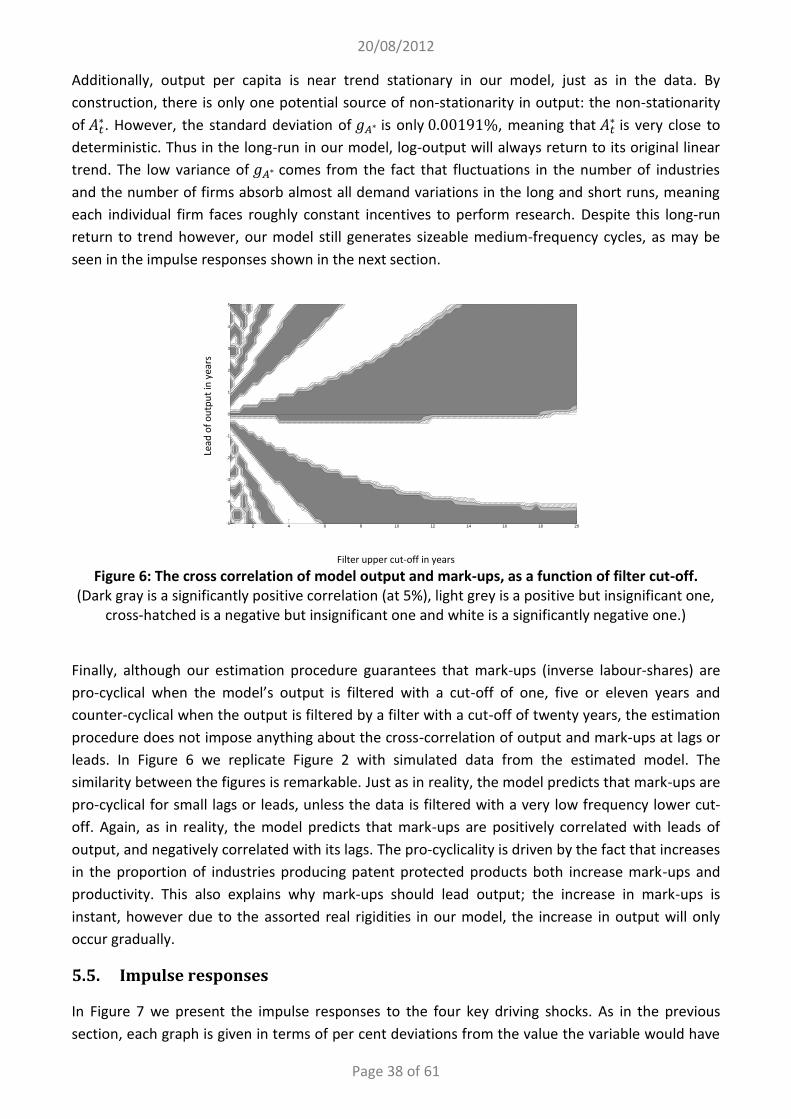
20/08/2012
Page 38 of 61
Additionally, output per capita is near trend stationary in our model, just as in the data. By
construction, there is only one potential source of non-stationarity in output: the non-stationarity
of . However, the standard deviation of is only , meaning that
is very close to
deterministic. Thus in the long-run in our model, log-output will always return to its original linear
trend. The low variance of comes from the fact that fluctuations in the number of industries
and the number of firms absorb almost all demand variations in the long and short runs, meaning
each individual firm faces roughly constant incentives to perform research. Despite this long-run
return to trend however, our model still generates sizeable medium-frequency cycles, as may be
seen in the impulse responses shown in the next section.
Filter upper cut-off in years
Figure 6: The cross correlation of model output and mark-ups, as a function of filter cut-off. (Dark gray is a significantly positive correlation (at 5%), light grey is a positive but insignificant one,
cross-hatched is a negative but insignificant one and white is a significantly negative one.)
Finally, although our estimation procedure guarantees that mark-ups (inverse labour-shares) are
pro-cyclical when the model’s output is filtered with a cut-off of one, five or eleven years and
counter-cyclical when the output is filtered by a filter with a cut-off of twenty years, the estimation
procedure does not impose anything about the cross-correlation of output and mark-ups at lags or
leads. In Figure 6 we replicate Figure 2 with simulated data from the estimated model. The
similarity between the figures is remarkable. Just as in reality, the model predicts that mark-ups are
pro-cyclical for small lags or leads, unless the data is filtered with a very low frequency lower cut-
off. Again, as in reality, the model predicts that mark-ups are positively correlated with leads of
output, and negatively correlated with its lags. The pro-cyclicality is driven by the fact that increases
in the proportion of industries producing patent protected products both increase mark-ups and
productivity. This also explains why mark-ups should lead output; the increase in mark-ups is
instant, however due to the assorted real rigidities in our model, the increase in output will only
occur gradually.
5.5. Impulse responses
In Figure 7 we present the impulse responses to the four key driving shocks. As in the previous
section, each graph is given in terms of per cent deviations from the value the variable would have
2 4 6 8 10 12 14 16 18 20-5
-4
-3
-2
-1
0
1
2
3
4
5
Lead
of
ou
tpu
t in
yea
rs

20/08/2012
Page 39 of 61
taken had the shock never arrived, and the horizontal axis shows time in years, though this is a
quarterly model. For no shocks was there an asymmetric positive and negative response, so the
lower bound on invention is irrelevant. Each shock is in a different column, and the key response
variables are in rows. Solid lines show the response with the estimated degree of wage stickiness,
dashed lines show responses under flexible wages.59
To show the magnitude of the effects of these shocks on productivity, we include the implied Solow
residual60 in the third row. Our chief driving shock, that to depreciation, has both a direct effect on
the Solow residual through reduced utilisation, and an indirect one through the consequent
reduction in invention and transfer away from new, highly productive industries, both of which
operate in the same direction initially. However, the indirect effect far outlasts the direct one, with
aggregate productivity still negative nearly twenty years after the original shock. It then slightly
overshoots due to our model’s real rigidities, producing a medium frequency cycle in productivity.
In fact, thanks to the model’s endogenous growth component, the Solow residual moves following
each of the four shocks, so in a sense all shocks are TFP shocks. Most interesting of these is our
monetary policy shock, as a large medium term impact of monetary policy on productivity would
substantially alter prescriptions for optimal monetary policy. Here we see that an unexpected
basis point increase in the nominal interest rate leads to a fall in productivity after twelve
years. Hence it would take a basis point surprise (i.e. ) to generate a movement in
aggregate productivity. Consequently, our model suggests that the medium term impacts of
monetary policy on productivity are not something that policy makers need to factor in to their
decisions.
59 In this case, we set to avoid numerical problems introduced in the limit.
60 The Solow residual is given by
( )
in the notation of the appendix, section 8.5.

20/08/2012
Page 40 of 61
Depreciation shock ( ) Negative labour supply shock ( )
Nom. interest shock (
) Population shock ( )
Figure 7: Impulse responses from the core model.
(Vertical axes are in percent, horizontal axes are in years. Solid lines are with nominal wage rigidity, dashed lines are with flexible wages.)
0 10 20 30 40 50
00.20.40.60.8
0 10 20 30 40 50
0
50
100
150
0 10 20 30 40 50
0
0.02
0.04
0.06
0 10 20 30 40 50
0
0.05
0.1
0 10 20 30 40 50
-0.8-0.6-0.4-0.2
0
0 10 20 30 40 50
-1
-0.5
0
0 10 20 30 40 50
-0.2
-0.1
0
0 10 20 30 40 50-0.06
-0.04
-0.02
0
0 10 20 30 40 50
-0.15
-0.1
-0.05
0
0 10 20 30 40 50
-0.02
-0.01
0
0.01
0 10 20 30 40 50
0
5
10
x 10-3
0 10 20 30 40 50-5
0
5
x 10-3
0 10 20 30 40 50
-0.08-0.06-0.04-0.02
00.020.04
0 10 20 30 40 50
-0.01
0
0.01
0 10 20 30 40 50
-1
0
1
x 10-3
0 10 20 30 40 50
0
2
4
x 10-3
0 10 20 30 40 50
-2
-1
0
0 10 20 30 40 50
-0.6
-0.4
-0.2
0
0 10 20 30 40 50
-0.08-0.06-0.04-0.02
00.02
0 10 20 30 40 50
-0.05
0
0.05
0 10 20 30 40 50
-0.4
-0.2
0
0 10 20 30 40 50-0.8
-0.6
-0.4
-0.2
0
0 10 20 30 40 50
-0.08
-0.06
-0.04
-0.02
0
0 10 20 30 40 50
-0.04
-0.02
0
0 10 20 30 40 50
-2
-1
0
0 10 20 30 40 50
-3
-2
-1
0
0 10 20 30 40 50
-0.6
-0.4
-0.2
0
0 10 20 30 40 50
-0.05
0
0.05
0 10 20 30 40 50
-0.4
-0.2
0
0 10 20 30 40 50
0
0.2
0.4
0 10 20 30 40 50
-0.06
-0.04
-0.02
0
0 10 20 30 40 50
0
5
10
x 10-3
0 10 20 30 40 50
-0.04
-0.02
0
0 10 20 30 40 50
0
0.02
0.04
0 10 20 30 40 50
0
2
4
x 10-3
0 10 20 30 40 50
0
1
2
x 10-3
0 10 20 30 40 50
-10
-5
0
5
x 10-3
0 10 20 30 40 50
-0.010
0.010.020.03
0 10 20 30 40 50
-4-202
x 10-3
0 10 20 30 40 50
0
10
20
x 10-4
0 10 20 30 40 50
-0.8-0.6-0.4-0.2
0
0 10 20 30 40 50
-1
-0.5
0
0 10 20 30 40 50
-0.2
-0.1
0
0 10 20 30 40 50
-0.04
-0.02
0
0 10 20 30 40 50
-0.15
-0.1
-0.05
0
0.05
0 10 20 30 40 50
-0.2
-0.1
0
0.1
0 10 20 30 40 50
-0.02
0
0.02
0.04
0.06
0 10 20 30 40 50-15
-10
-50
5
x 10-3
The shock
Solow residual
Aggregate prod. (𝐴𝑡)
Consumption
per capita (𝐶𝑡
𝑁𝑡)
R&D exp. per capita
Output per
capita (𝑌𝑡
𝑁𝑡)
Inv. per capita (𝐼𝑡
P 𝜚GDP𝐼𝑡R)
Consumption price (𝑃𝑡)
Real interest rate (𝑅𝑡)
Lab. sup. per
capita (𝐿𝑡
𝑁𝑡)
Real wage (𝑊𝑡)
Nom. interest rate (𝑅𝑡
)

20/08/2012
Page 41 of 61
6. Conclusion
Many have expressed the worry that “the apparent fit of the DSGE model [has] more to do with the
inclusion of suitable exogenous driving processes than with the realism of the model structure
itself”61. In this paper, we have demonstrated that if productivity is endogenized through research,
appropriation and invention then even a frictionless RBC model is capable of generating rich
persistent dynamics from uncorrelated shocks, and a full medium-scale model is capable of
accurately matching key moments, providing a statistically significant improvement in model fit.
We showed that all shocks lead to changes in the rate of product invention that have significant
consequences for aggregate productivity and mark-ups at medium-frequency, due to fluctuations in
the proportion of industries that are producing patent-protected products. Our model’s
propagation mechanisms thus lend persistence to all shocks, not just shocks to the invention or
research process. Furthermore, this improvement in the model’s propagation mechanism does not
come at the expense of counter-factual movements in mark-ups, implausibly large unit roots in
output, or the use of a growth model that we can reject thanks to the absence of strong scale
effects in the data. In all of these respects, then, our model presents a substantial advance on the
prior literature.
The fact we are able to combine a plausible growth model with a business cycle model also enables
us to get much tighter estimates of the strength of externalities (for example) than is possible from
traditional growth models, since these parameters have an impact on the dynamics as well as on
the long run growth rate. This will enable the testing of hypotheses about the mechanics of
endogenous growth that were previously near impossible to test.
Our model suggests that a switch to indefinite patent protection would result in significant welfare
improvements. Such a switch would both permanently increase the level of aggregate productivity,
and substantially lessen its variance and persistence, while only slightly increasing mark-ups and
efficiency losses due to research duplication. Indeed, it may be shown that in our model increasing
patent protection even slightly increases growth rates, as industry profits are decreasing in
aggregate productivity, and so with indefinite patent protection each (protected) industry has
fewer firms meaning higher mark-ups and higher research. However, it is clear that the structure of
our model has “stacked-the-deck” in favour of finding a beneficial role for patent protection.
Patents in our model are less broad than in the real world, and they do not hinder future research
or invention. One minimal conclusion we can draw on patent protection is that product patents
should at least be long enough that by the end of patent protection, production process have
reached frontier productivity. In our model, this time goes to zero asymptotically. A less radical
policy change might be to grant temporary extensions to patents that would otherwise expire
during a recession. We intend to explore the full policy implications of this model in future work.
61 Del Negro et al. (2007) paraphrasing Kilian (2007).

20/08/2012
Page 42 of 61
7. References
Adjemian, Stéphane, Houtan Bastani, Michel Juillard, Ferhat Mihoubi, George Perendia, Marco Ratto, and Sébastien Villemot. 2011. Dynare: Reference Manual, Version 4. Dynare Working Papers. CEPREMAP, April. http://ideas.repec.org/p/cpm/dynare/001.html.
Aghion, Philippe, Nick Bloom, Richard Blundell, Rachel Griffith, and Peter Howitt. 2005. Competition and Innovation: An Inverted-U Relationship. Quarterly Journal of Economics 120, no. 2 (May): 701–728.
Aghion, Philippe, and Peter Howitt. 1992. A Model of Growth Through Creative Destruction. Econometrica 60, no. 2 (March): 323–351.
Andrews, Donald W. K. 1991. Heteroskedasticity and Autocorrelation Consistent Covariance Matrix Estimation. Econometrica 59, no. 3 (May 1): 817–858.
Autor, David H, Lawrence F Katz, and Melissa S Kearney. 2008. Trends in U.S. Wage Inequality: Revising the Revisionists. Review of Economics and Statistics 90, no. 2: 300–323.
Bachmann, Ruediger, and Christian Bayer. 2009. The Cross-section of Firms over the Business Cycle: New Facts and a DSGE Exploration. CESifo Group Munich. http://ideas.repec.org/p/ces/ceswps/_2810.html.
Balasubramanian, Natarajan, and Jagadeesh Sivadasan. 2011. What Happens When Firms Patent? New Evidence from U.S. Economic Census Data. Review of Economics and Statistics 93, no. 1 (July 7): 126–146.
Barattieri, Alessandro, Susanto Basu, and Peter Gottschalk. 2010. Some Evidence on the Importance of Sticky Wages. NBER Working Papers. National Bureau of Economic Research, Inc. http://ideas.repec.org/p/nbr/nberwo/16130.html.
Bental, Benjamin, and Dan Peled. 1996. The Accumulation of Wealth and the Cyclical Generation of New Technologies: A Search Theoretic Approach. International Economic Review 37, no. 3 (August): 687–718.
Bilbiie, Florin O., Fabio Ghironi, and Marc J Melitz. 2011. Endogenous Entry, Product Variety, and Business Cycles. CEPR Discussion Papers. C.E.P.R. Discussion Papers, September. http://ideas.repec.org/p/cpr/ceprdp/8564.html.
Bilbiie, Florin O., Fabio Ghironi, and Marc J. Melitz. 2007. Monetary Policy and Business Cycles with Endogenous Entry and Product Variety. National Bureau of Economic Research Working Paper Series No. 13199 (June). http://www.nber.org/papers/w13199.
———. 2008. Monopoly Power and Endogenous Product Variety: Distortions and Remedies. NBER Working Papers. National Bureau of Economic Research, Inc, October. http://ideas.repec.org/p/nbr/nberwo/14383.html.
Bils, Mark. 1998. Discussion of Basu (1998). Conference Series ; [Proceedings], no. Jun. http://www.bos.frb.org/economic/conf/conf42/con42_14.pdf.
Bonanno, Giacomo. 1988. Oligopoly Equilibria When Firms Have Local Knowledge of Demand. International Economic Review 29, no. 1 (February 1): 45–55.
Boulhol, Hervé. 2007. The Convergence of Price–cost Margins. Open Economies Review 19, no. 2 (May): 221–240.
Broda, Christian, and David E Weinstein. 2010. Product Creation and Destruction: Evidence and Price Implications. American Economic Review 100, no. 3 (June): 691–723.
Calvo, Guillermo A. 1983. Staggered Prices in a Utility-Maximizing Framework. Journal of Monetary Economics 12, no. 3: 383–398.
Campbell, Jeffrey R. 1998. Entry, Exit, Embodied Technology, and Business Cycles. Review of Economic Dynamics 1, no. 2 (April): 371–408.
Candès, Emmanuel, Michael Wakin, and Stephen Boyd. 2008. Enhancing Sparsity by Reweighted ℓ1 Minimization. Journal of Fourier Analysis and Applications 14, no. 5 (December 1): 877–905.

20/08/2012
Page 43 of 61
Canova, Fabio. 2009. Bridging cyclical DSGE models and the raw data. August 28. http://www.crei.cat/people/canova/dsge_trend(1).pdf.
Chari, V. V., Patrick J. Kehoe, and Ellen R. McGrattan. 2009. New Keynesian Models: Not Yet Useful for Policy Analysis. American Economic Journal: Macroeconomics 1, no. 1: 242–66.
Cheung, Yin-Wong, and Kon S. Lai. 1995. Lag Order and Critical Values of the Augmented Dickey-Fuller Test. Journal of Business & Economic Statistics 13, no. 3 (July 1): 277–280.
Christiano L., and Fitzgerald T. 2003. The Band Pass Filter. International Economic Review 44 (May): 435–465.
Christiano, Lawrence J., Martin Eichenbaum, and Charles L. Evans. 2005. Nominal Rigidities and the Dynamic Effects of a Shock to Monetary Policy. Journal of Political Economy 113, no. 1: 1–45.
Cochrane, John H. 1988. How Big Is the Random Walk in GNP? Journal of Political Economy 96, no. 5 (October 1): 893–920.
Comin, Diego. 2009. On the integration of growth and business cycles. Empirica 36, no. 2 (May 1): 165–176.
Comin, Diego, and Mark Gertler. 2006. Medium-Term Business Cycles. American Economic Review 96, no. 3 (June): 523–551.
Comin, Diego, Mark Gertler, and Ana Maria Santacreu. 2009. Technology Innovation and Diffusion as Sources of Output and Asset Price Fluctuations. National Bureau of Economic Research, Inc, June. RePEc. http://ideas.repec.org/p/nbr/nberwo/15029.html.
Comin, Diego, and Sunil Mulani. 2009. A theory of growth and volatility at the aggregate and firm level. Journal of Monetary Economics 56, no. 8 (November): 1023–1042.
Diewert, W. E. 1978. Superlative Index Numbers and Consistency in Aggregation. Econometrica 46, no. 4 (July 1): 883–900.
Dixit, Avinash K., and Joseph E. Stiglitz. 1977. Monopolistic Competition and Optimum Product Diversity. The American Economic Review 67, no. 3 (June): 297–308.
Doornik, Jurgen A, and Henrik Hansen. 2008. An Omnibus Test for Univariate and Multivariate Normality*. Oxford Bulletin of Economics and Statistics 70 (December 1): 927–939.
Duarte, Margarida, and Diego Restuccia. 2009. The Role of the Structural Transformation in Aggregate Productivity. Working Papers tecipa-348. University of Toronto, Department of Economics. http://ideas.repec.org/p/tor/tecipa/tecipa-348.html.
Dueker, Michael, Andreas Fischer, and Robert Dittmar. 2007. Stochastic Capital Depreciation and the Co-movement of Hours and Productivity. The B.E. Journal of Macroeconomics 0, no. 3: 6.
Eaton, Jonathan, and Samuel Kortum. 1999. International Technology Diffusion: Theory and Measurement. International Economic Review 40, no. 3 (August 1): 537–570.
Eisfeldt, Andrea L., and Adriano A. Rampini. 2006. Capital reallocation and liquidity. Journal of Monetary Economics 53, no. 3 (April): 369–399.
Ellis, Colin. 2006. Elasticities, Markups and Technical Progress: Evidence from a State-Space Approach. SSRN. http://ssrn.com/paper=932580.
Erceg, Christopher J., Dale W. Henderson, and Andrew T. Levin. 2000. Optimal monetary policy with staggered wage and price contracts. Journal of Monetary Economics 46, no. 2 (October): 281–313.
Ethier, Wilfred J. 1982. National and International Returns to Scale in the Modern Theory of International Trade. The American Economic Review 72, no. 3 (June): 389–405.
Forni, Mario, and Sergio Paba. 2002. Spillovers and the growth of local industries. The Journal of Industrial Economics 50, no. 2 (June 1): 151–171.
Francois, Patrick, and Huw Lloyd-Ellis. 2009. Schumpeterian cycles with pro-cyclical R&D. Review of Economic Dynamics 12, no. 4 (October): 567–591.
Francois, Patrick, and Huw Lloyd‐Ellis. 2008. Implementation cycles, investment, and growth. International Economic Review 49, no. 3 (August 1): 901–942.

20/08/2012
Page 44 of 61
Furlanetto, Francesco, and Martin Seneca. 2011. New perspectives on depreciation shocks as a source of business cycle fluctuations. Working Paper. Norges Bank, March. http://ideas.repec.org/p/bno/worpap/2011_02.html.
Ginarte, Juan C., and Walter G. Park. 1997. Determinants of patent rights: A cross-national study. Research Policy 26, no. 3 (October): 283–301.
Griliches, Zvi. 1998. The Search for R&D Spillovers. NBER Chapters. National Bureau of Economic Research, Inc. http://www.nber.org/chapters/c8349.pdf.
Groth, Christian, Karl-Josef Koch, and Thomas Steger. 2009. When economic growth is less than exponential. Economic Theory (July 4). http://dx.doi.org/10.1007/s00199-009-0480-y.
Hansen, N., A.S.P. Niederberger, L. Guzzella, and P. Koumoutsakos. 2009. A Method for Handling Uncertainty in Evolutionary Optimization With an Application to Feedback Control of Combustion. Evolutionary Computation, IEEE Transactions on 13, no. 1: 180–197.
Hart, Oliver, and John Moore. 1994. A Theory of Debt Based on the Inalienability of Human Capital. The Quarterly Journal of Economics 109, no. 4 (November 1): 841–879.
Head, Allen, Lucy Qian Liu, Guido Menzio, and Randall Wright. 2011. Sticky Prices: A New Monetarist Approach. NBER Working Paper. National Bureau of Economic Research, Inc. http://ideas.repec.org/p/nbr/nberwo/17520.html.
Heston, Alan, Robert Summers, and Bettina Aten. 2011. Penn World Table Version 7.0. Center for International Comparisons of Production, Income and Prices at the University of Pennsylvania, May. http://pwt.econ.upenn.edu/php_site/pwt_index.php.
Hodrick, Robert J., and Edward C. Prescott. 1997. Postwar U.S. Business Cycles: An Empirical Investigation. Journal of Money, Credit and Banking 29, no. 1 (February): 1–16.
Holden, Tom. 2011. Products, patents and productivity persistence: A DSGE model of endogenous growth. Dynare Working Papers. CEPREMAP, May. http://ideas.repec.org/p/cpm/dynare/004.html.
Horii, Ryo. 2011. Wants and past knowledge: Growth cycles with emerging industries. Journal of Economic Dynamics and Control In Press, Accepted Manuscript. http://www.sciencedirect.com/science/article/pii/S0165188911001436.
Hurvich, Clifford M. 1985. Data-Driven Choice of a Spectrum Estimate: Extending the Applicability of Cross-Validation Methods. Journal of the American Statistical Association 80, no. 392 (December 1): 933–940.
Jaimovich, Nir. 2007. Firm dynamics and markup variations: Implications for sunspot equilibria and endogenous economic fluctuations. Journal of Economic Theory 137, no. 1 (November): 300–325.
Jaimovich, Nir, and Sergio Rebelo. 2008. News and Business Cycles in Open Economies. Journal of Money, Credit and Banking 40, no. 8: 1699–1711.
———. 2009. Can News about the Future Drive the Business Cycle? American Economic Review 99, no. 4 (September): 1097–1118.
Justiniano, Alejandro, Giorgio E. Primiceri, and Andrea Tambalotti. 2011. Investment shocks and the relative price of investment. Review of Economic Dynamics 14, no. 1 (January): 102–121.
Kehrig, Matthias. 2011. The Cyclicality of Productivity Dispersion. Center for Economic Studies, U.S. Census Bureau, May. http://ideas.repec.org/p/cen/wpaper/11-15.html.
Kilian, Lutz. 2007. Comment. Journal of Business & Economic Statistics 25. Journal of Business & Economic Statistics: 156–159.
Kim, Bae-Geun. 2010. Identifying a permanent markup shock and its implications for macroeconomic dynamics. Journal of Economic Dynamics and Control (April 14). http://dx.doi.org/10.1016/j.jedc.2010.04.003.
Kiyotaki, Nobuhiro, and John Moore. 1997. Credit Cycles. Journal of Political Economy 105, no. 2 (April 1): 211–248.

20/08/2012
Page 45 of 61
Klenow, Peter J., and Andrés Rodríguez-Clare. 2005. Chapter 11 Externalities and Growth. In Handbook of Economic Growth, Volume 1, Part A:817–861. Vol. Volume 1, Part A. Elsevier. http://www.sciencedirect.com/science/article/pii/S1574068405010117.
Lee, Anthony, Francois Caron, Arnaud Doucet, and Chris Holmes. 2010. A Hierarchical Bayesian Framework for Constructing Sparsity-inducing Priors. arXiv:1009.1914 (September 9). http://arxiv.org/abs/1009.1914.
Levin, Richard C., Wesley M. Cohen, and David C. Mowery. 1985. R & D Appropriability, Opportunity, and Market Structure: New Evidence on Some Schumpeterian Hypotheses. The American Economic Review 75, no. 2 (May): 20–24.
Levy, Daniel, and Hashem Dezhbakhsh. 2003. International evidence on output fluctuation and shock persistence. Journal of Monetary Economics 50, no. 7 (October): 1499–1530.
Litterman, Robert B. 1983. A Random Walk, Markov Model for the Distribution of Time Series. Journal of Business & Economic Statistics 1, no. 2. Journal of Business & Economic Statistics: 169–73.
Liu, Zheng, Daniel F Waggoner, and Tao Zha. 2011. Sources of macroeconomic fluctuations: A regime‐switching DSGE approach. Quantitative Economics 2, no. 2 (July 1): 251–301.
Matsuyama, Kiminori. 1999. Growing Through Cycles. Econometrica 67, no. 2 (March): 335–347. Del Negro, Marco, Frank Schorfheide, Frank Smets, and Rafael Wouters. 2007. Rejoinder. Journal of
Business and Economic Statistics 25, no. 2: 159. Nekarda, Christopher, and Valerie Ramey. 2010. The Cyclical Behavior of the Price-Cost Markup.
http://econ.ucsd.edu/~vramey/research/markupcyc.pdf. Nuño, Galo. 2008. Schumpeterian Foundations of Real Business Cycles. Working Papers.
International Economics Institute, University of Valencia, December. http://ideas.repec.org/p/iei/wpaper/0805.html.
———. 2009. Technology, convergence and business cycles. Banco de España, October. http://ideas.repec.org/p/bde/wpaper/0922.html.
———. 2011. Optimal research and development and the cost of business cycles. Journal of Economic Growth 16, no. 3 (April 26): 257–283.
Pavlov, Oscar, and Mark Weder. 2012. Variety matters. Journal of Economic Dynamics and Control 36, no. 4 (April): 629–641.
Peretto, Pietro F. 1999. Cost reduction, entry, and the interdependence of market structure and economic growth. Journal of Monetary Economics 43, no. 1 (February 19): 173–195.
Phillips, Kerk L., and Jeff Wrase. 2006. Is Schumpeterian `creative destruction’ a plausible source of endogenous real business cycle shocks? Journal of Economic Dynamics and Control 30, no. 11 (November): 1885–1913.
Pincus, Laura B. 1991. Computation of Damages in Patent Infringement Actions. Harvard Journal of Law & Technology 5: 95.
La Porta, Rafael, Florencio Lopez-de-Silanes, and Andrei Shleifer. 2008. The Economic Consequences of Legal Origins. Journal of Economic Literature 46, no. 2. Journal of Economic Literature: 285–332.
Ramsey, J. B. 1969. Tests for Specification Errors in Classical Linear Least-Squares Regression Analysis. Journal of the Royal Statistical Society. Series B (Methodological) 31, no. 2 (January 1): 350–371.
Rubinstein, Ariel. 1982. Perfect Equilibrium in a Bargaining Model. Econometrica 50, no. 1 (January): 97–109.
Said, Said E., and David A. Dickey. 1984. Testing for Unit Roots in Autoregressive-Moving Average Models of Unknown Order. Biometrika 71, no. 3 (December 1): 599–607.
Schmitt-Grohé, Stephanie, and Martín Uribe. 2006. Comparing Two Variants of Calvo-Type Wage Stickiness. NBER Working Paper. National Bureau of Economic Research, Inc. http://ideas.repec.org/p/nbr/nberwo/12740.html.

20/08/2012
Page 46 of 61
———. 2011. Business cycles with a common trend in neutral and investment-specific productivity. Review of Economic Dynamics 14, no. 1 (January): 122–135.
Scott, John. 1984. Firm versus Industry Variability in R&D Intensity. In R & D, Patents, and Productivity. NBER, January 1. http://www.nber.org/chapters/c10051.
Serrano, C. J. 2007. Technology Transfer and the Business Cycle: Evidence from Patent Reassignments. http://homes.chass.utoronto.ca/~serrano/papers/RBCpatent.pdf.
Serrano, Carlos J. 2010. The dynamics of the transfer and renewal of patents. The RAND Journal of Economics 41, no. 4 (December 1): 686–708.
The Associated Press. 2008. Court Rules Business Concept Cannot Be Patented. The New York Times, October 31, sec. Business. http://www.nytimes.com/2008/10/31/business/31patent.html?_r=1.
Tingvall, Patrik Gustavsson, and Andreas Poldahl. 2006. Is there really an inverted U-shaped relation between competition and R&D? Economics of Innovation and New Technology 15, no. 3: 101.
Wälde, Klaus. 2005. Endogenous Growth Cycles. International Economic Review 46, no. 3: 867–894. White, Halbert. 1980. A Heteroskedasticity-Consistent Covariance Matrix Estimator and a Direct
Test for Heteroskedasticity. Econometrica 48, no. 4 (May 1): 817–838. Woodford, Michael. 2001. The Taylor Rule and Optimal Monetary Policy. The American Economic
Review 91, no. 2 (May 1): 232–237.
8. Online appendices
8.1. The free-entry and first order conditions
When deciding how much research and appropriation to perform, firms realise that if they perform
a non-equilibrium amount then in the next period they will have an incentive to set a different
mark-up to the other firms in their industry. (The clearest example of this is when we have perfect
competition, in which case the most productive firm would want to price just below the second
most productive firms’ marginal cost.) It may be seen that in non-symmetric equilibrium the
optimal price satisfies:
( )
( )
[
( )
( )( ( )
( ))
]
Since we are looking for a symmetric equilibrium, it is sufficient to approximate this locally around
( ) ( ) in order to calculate firms’ research and appropriation incentives. Taking a log-
linear approximation of ( ) in ( )
( ) gives us that:
( )
( )( ( )) (
( )
( ))
( )

20/08/2012
Page 47 of 61
where ( ) ( )( )
( ( ) ( )) ( ( ))
captures the strength of these incentives to deviate from
setting the same mark-up as all other firms in their industry. Therefore ( )
( )( ( ))
and ( )
( )( ( )) (
( )
( ))
( )
( ) where:
( ) [
( )∑ ( )
( ( ))
( )
]
( ( ))
Therefore, up to a first order approximation around the symmetric solution, profits are given by:
( )( ( )
)
[( ( )
( ))
( )
( )
( )] ( ( )
( ))
( )
( ( ))
( ( )
)
[ ( )
( ) ( ) ]
Note that if ( ) √ ( √ )
√ , then ( ) (by tedious algebra), so providing
there are at least two firms in the industry, this expression is guaranteed to be increasing and
concave in ( ).
Let ( ) be the Lagrange multiplier on research’s positivity constraint and
( ) be the
Lagrange multiplier on appropriation’s positivity constraint. Then in a symmetric equilibrium the
two first order conditions and the free entry condition (respectively) mean:
( )
( )
( )( ( )
)
( ( )
)
( )
( )
( )
( )
( )
( ( ))
( )
( )
( )( ( )
)
( ( )
)
( )
( )
( ) ( )
( )
( )
( )
( ) (
( ) )
( ) ( ( )
( )) (
( ))
( )
( )
( )( ( )
)
( ( )
)
[ ( )
( ) ( )
]
where:
( ) ( )
( )
( ( ))( ( ) )
( ) ( )
and where we have dropped indices on variables which are the same across the industry. We also
have that:

20/08/2012
Page 48 of 61
( ( ))( ( ) )
( ) ( ) ( √ )(√ )
√
so providing , ( ) .
That the solution for research when is given by equation (3.2) is a trivial consequence of
the complementary slackness condition and the facts that
( ) and ( ) . Deriving (3.3) is
less trivial though.
Begin by defining ( ) ( )
( )
( )
, and note that since we are assuming , we have
that ( ) .
Also define:
( ) ( ) ( )
( ) ( )
[(
( )
)
] [ ( )
( ) ]
which is not a function of ( ), given
( ).
We can then combine the appropriation first order condition with the free entry condition to
obtain:
( ( ))
( ( )
( )
)
[ ( ) ( )
( )[(
( )
)
] ( ) ( )]
( )
Since the left hand side is weakly positive, from the dual feasibility condition we know ( )
[ ]. Now when ( ) , this becomes:
( ) ( )
since in this case ( )
( ). Therefore when ( ) , ( ) .
We now prove the converse. Suppose then for a contradiction that ( ) , but ( ) . By
complementary slackness we must have ( ) , hence:
( ) ( ( ))
( ( )
( )
)
( ) ( )
( )[(
( )
)
] ( )
( ( ))
( ( )
( )
)
[(
( )
)
] ( )
( ( )) [(
( )) ( ) [(
( )
)
]] [(
( )
)
] ( )
where we have used the facts that ( ) ( ) and
( ) to derive the second inequality.
20/08/2012
Page 49 of 61
Expanding the brackets then gives that:
( ) (
( )
)
( )
i.e. that (
( ))
( ) which is a contradiction as (
( ))
( ) .
We have proven then that providing
( ) ,
( ) if and only if ( ) . It just remains for
us to solve for ( ) when it is strictly positive. From the above, we have that, in this case:
( ( )
)
[ ( ) ] [
[
( ) ( )
( )] [ (
( )
)
]] ( )
( )
Hence:
( ) [
[
( ) ( )
( )] [ (
( )
)
]]
√[
[
( ) ( )
( )] [ (
( )
)
]]
( ( )
)
[ ( ) ]
since the lower solution is guaranteed to be negative as ( ) when ( ) .
8.2. The steady state for non-patent-protected industries
In an industry which is not patent-protected and in which appropriation, but no research, is
performed, from (3.1) and (3.3):
( ) √ ( ) ( ) ( ) [
( ( )
( )
)
( ( )
)
( ( )
)
]
If we treat ( )
( ) ,
( )
and ( ( )
( )
)
as fixed, this
leaves us with a cubic in ( ( )
)
, for which only one solution will be feasible (i.e. strictly less than
). Taking a second order Taylor approximation of this solution in , and , reveals (after some
messy computation), that:
( ( )
)
( ( )) ( )
( ( )
( )
( )
)
(The effect of on ( ( )
)
is third order and hence it does not appear in this expression.)

20/08/2012
Page 50 of 61
From this approximate solution for ( ( )
)
then, we have that the relative productivity of a non-
protected industry is decreasing in its mark-up. Furthermore, from dropping to a first order
approximation, we have that ( )
(
)
, so asymptotically non-protected industries are
growing at [
]
times the growth rate of the frontier.
8.3. The inventor-firm bargaining process
We model the entire process of setting and paying rents as follows:
1) Firms enter, paying the fixed cost.
2) Firms who have entered conduct appropriation, then research.
3) The “idea shock” for next period’s production, , is realised and firms and patent holders
learn its level.
4) Finally, firms arrive at the patent-holder to conduct bargaining, with these arrivals taking place
sequentially but in a random order. (For example, all firms phone the patent-holder sometime
in the week before production is to begin.) In this bargaining we suppose that the patent-holder
has greater bargaining power, since they have a longer outlook62 and since they lose nothing if
bargaining collapses63. We also suppose that neither patent-holders nor firms are able to
observe or verify either how many (other) firms paid the fixed cost or what research and
appropriation levels they chose. This is plausible because until production begins it is relatively
easy to keep such things hidden (for example, by purchasing the licence under a spin-off
company), and because it is hard to ascertain ahead of production exactly what product a firm
will be producing. We assume bargaining takes an alternating offer form, (Rubinstein 1982) but
that it happens arbitrarily quickly (i.e. in the no discounting limit).
5) Firms pay the agreed rents if bargaining was successful. Since this cost is expended before
production, we continue to suppose firms have to borrow in the period before production in
order to cover it. Firms will treat it as a fixed cost, sunk upon entry, since our unobservability
assumptions mean bargaining’s outcome will not be a function of research and appropriation
levels.
6) The next period starts, other aggregate shocks are realised and production takes place.
62 Consider what happens as the time gap between offers increases. When this gap is large enough only one offer would
be made per-period, meaning the patent-holder would make a take-it-or-leave-it offer giving (almost) nothing to the
firm, which the firm would then accept. 63
The firm owner may, for example, face restrictions from starting businesses in future if as a result of the bargaining
collapse they are unable to repay their creditors.

20/08/2012
Page 51 of 61
7) The patent-holder brings court cases against any firms who produced but decided not to pay
the rent. For simplicity, we assume the court always orders the violating firm to pay damages to
the patent-holder, which are given as follows:
a) When the courts believe rents were not reasonable (i.e. ( )
( ), where ( ) is
the level courts determine to be “reasonable royalties”), they set damages greater than
( ) , as “the infringer would have nothing to lose, and everything to gain if he could
count on paying only the normal, routine royalty non-infringers might have paid”64. We
assume excess damages over ( ) are less than the patent-holder’s legal costs
however.
b) When the courts consider the charged rent to have been reasonable (i.e. ( )
( ))
the courts award punitive damages of more than { ( ) (
)
( ) }, where
is the bargaining power of the firm, in the sense of the generalized Nash bargaining
solution.65
Under this specification:
( ) {
( ) ( )[ ( )
( ) ( ) ]}
since entry is fixed when bargaining takes place, since patent-holders know that bargaining to a
rent level any higher than ( ) will just result in them having to pay legal costs,66 and since
[ ( )
( ) ( ) ] is equal to the production period profits of each firm in industry ,
by the free entry condition.67 Therefore, in equilibrium:
( ) {
( ) ( )} (8.1)
where ( ) is a solution to equations (3.2), (3.3) along with equation (3.4), (i.e.
( )
[ ( )
( ) ]) if one exists, or otherwise. Because damages are always greater than
( ) , these rents will be sufficiently low to ensure firms are always prepared to licence the
patent at the bargained price in equilibrium.
Now suppose we are out of equilibrium and fewer firms than expected have entered. Since neither
the patent-holder nor firms can observe how many firms have entered, and since firms arrive at the
patent-holder sequentially, both sides will continue to believe that the equilibrium number of firms
64 Panduit Corp. v. Stahlin Brothers Fibre Works, Inc., 575 F.2d 1152, 1158 (6th Circuit 1978), cited in Pincus (1991).
65 The level (
)
( ) is chosen to ensure that, with equilibrium rents, firms prefer not to produce at all rather
than to produce without paying rents. 66
The disagreement point is zero since it is guaranteed that ( )
( ) and so punitive damages would be awarded
were the firm to produce without paying rents, which, by construction, leaves them worse off than not producing. 67
A similar expression can also be derived if we assume instead that courts guarantee infringers a fraction of
production profits, or if we assume courts always award punitive damages but firms are able to hide a fraction of
their production profits.

20/08/2012
Page 52 of 61
has entered and so rents will not adjust. On the other hand, suppose that (out of equilibrium) too
many firms enter. When the first unexpected firm arrives at the patent-holder to negotiate, the
patent-holder will indeed realise that too many firms have entered. However, since the firm they
are bargaining with has no way of knowing this,68 the patent-holder can bargain for the same rents
as in equilibrium. Therefore, even out of equilibrium:
( ) {
( ) ( )}
where we stress ( ) is not a function of the decisions any firm happened to take. This ensures
that any solution of equations (3.2), (3.3) and (8.1) for research, appropriation and rents will also be
an equilibrium, even allowing for the additional condition that the derivative of firm profits with
respect to the number of firms must be negative at an optimum.
We now just have to pin down “reasonable royalties”, ( ) . Certainly it must be the case that
( )
( ), where ( ) is the level of rents at which ( ) , since rents so high that no one
is prepared to pay them must fall foul of the courts’ desire to ensure licensees can make a profit. 69
However, since when ( ) the sole entering firm (almost) may as well be the patent-holder
themselves, where possible the courts will set ( ) sufficiently low to ensure that ( ) in
equilibrium, again following the idea that licensees ought to be able to make a profit. When there is
a ( ) solution to equations (3.2), (3.3) and (3.4) already (i.e. ( ) ), the courts will just
set ( ) at the rent level that would obtain in that solution, thus preventing the possibility of
( ) being an equilibrium. It may be shown that for sufficiently large such a solution is
guaranteed to exist, so in this case ( )
( ) ( ).70
8.4. The de-trended model
Below we give the equations of the stationary model to which the model described in section 3
converges as .
68 Either they are a firm that thinks the equilibrium number of firms has entered, or they are a firm that thinks more
than the equilibrium number of firms has entered, but that does not know whether the patent-holder has yet realised
this. 69
“…the very definition of a reasonable royalty assumes that, after payment, the infringer will be left with a profit.”
Georgia-Pacific Corp. v. U.S. Plywood-Champion Papers Corp., 446 F.2d 295, 299 & n.1 (2d Cir.), cert. denied, 404 U.S.
870 (1971), cited in Pincus (1991). 70
There may still be multiple solutions for rents (as (3.2), (3.3) and (3.4) might have multiple solutions), but of these
only the one with minimal entry is really plausible, since this is both weakly Pareto dominant (firms always make zero
profits and it may be shown that the patent-holder prefers minimal entry) and less risky for entering firms (if entering
firms are unsure if the patent-holder will play the high rent or the low rent equilibrium, they are always better off
assuming the high rent one since if that assumption is wrong they make strict profits, whereas had they assumed low
rents but rents were in fact high they would make a strict loss).

20/08/2012
Page 53 of 61
8.4.1. Households
Stochastic discount factor:
, where
is consumption per person in
labour supply units and is the exponent of the growth rate of the variable at .
Labour supply:
, where
is labour supply per person and
is the wage
per effective unit of labour supply.
Euler equation: [ ] , where is the real interest rate.
8.4.2. Aggregate relationships
Aggregate mark-up pricing:
where is the aggregate mark-up in period .
Mark-up aggregation: (
)
(
)
(
)
( ), where ( ) is the mark-
up in any protected industry at , and ( )
is the proportion of
industries that will produce a patent protected product in period .
Productivity aggregation: (
)
(
)
(
)
( ), where
is
aggregate productivity relative to the frontier71 and
[(
)
(
( )) (
)
(
( ))]
is the aggregate relative
productivity of non-protected industries.
8.4.3. Firm decisions
Strategic in-industry pricing:
( )
, where ( ) is the number of firms in a
protected industry performing research at .
Firm research decisions:
(
)
, where
is the amount of effective research conducted by firms in protected industries
is the value of ( ) in protected industries and is the aggregate research-return shock.
(This equation means that
.)
Research and appropriation payoff: ( )
.
71 As a consequence, we have that
.

20/08/2012
Page 54 of 61
Free entry of firms:
(
)
, where
is the
measure of products relative to its trend,72 and
is output per person in labour supply
units.
8.4.4. Inventor decisions
Inventor profits: are given recursively by:
( )
, where
.
Free entry of inventors: Either binds or does.
8.4.5. Market clearing
Labour market clearing:
(
)
[(
)
(
)
(
)
(
)
( )].
Goods market clearing: .
8.5. The extended de-trended model
Define
( )( ), ( )( ) , (
) ( ) ,
and make the normalisation .
8.5.1. Households
Budget constraint Lagrange multiplier:
, where
is the Lagrange multiplier on the budget constraint and
.
Stochastic discount factor:
.
Labour supply: ( )
, where
[
(
)
]
(
is the real wage set by a household that updates its wage at ),
, and
72 This means
.

20/08/2012
Page 55 of 61
where and are the sums of costs and benefits respectively from the wage setting first
order conditions.73
Euler equation: [ ] .
Investment decisions: for { }:
( )[ ( )
( )]
( )
( ) , where
and
Utilisation decisions: for { }:
( )
[
(
)
( )
].
Capital accumulation: for { } : ( (
))
[
( )], where
and
(hence
).
8.5.2. Aggregate relationships
Aggregate mark-up pricing: [
]
( )
[ ( )
]
where
[ (
)]
and
.
Mark-up aggregation: (
)
(
)
(
)
( ) , where ( ) and
( )
.
Productivity aggregation: (
)
(
)
(
)
( ), where
and
[(
)
(
( )) (
)
(
( ))]
.
73 (
)
(
)
(
)
,
(
)
, where
and
. This formulation avoids
any explicit log-linearization and allows us to compute arbitrarily high order approximations to the model, for
robustness checks. A similar formulation is used in Schmitt-Grohé and Uribe (2006).

20/08/2012
Page 56 of 61
8.5.3. Firm decisions
Strategic in-industry pricing:
( )
, where ( ).
Firm research decisions:
(
)
, where
[
]
is the amount of effective research conducted by firms in
protected industries.
Research and appropriation payoff: ( )
.
Free entry of firms:
(
)
, where
( )
( )
is the measure of products relative to its trend,74
is gross output relative to
trend and [
]
( )
[ ( )
]
is the marginal cost of a unit of research or
invention, divided by
(where
[ (
)]
and
).
8.5.4. Inventor decisions
Inventor profits: are given recursively by:
( )
, where
.
Free entry of inventors: Either binds or does.
8.5.5. Market clearing
R&D expenditure: [ (
)
].
Labour market clearing:
. (
.)
Production labour market clearing:
( )( ) where
(
)
(
)
is a weighted measure of average inverse gross mark-
ups.
R&D labour market clearing:
( )( ) .
74 This means
( ) ( )
.

20/08/2012
Page 57 of 61
Capital markets clearing:
( )
,
( )
Goods market clearing: ( ) ( )
,
where is GDP over
and specifies the proportion of R&D capital investment that
is measured in GDP. (Given R&D itself is not measured in GDP it is not obvious that this equals
.)
Monetary rule:
(
)
[(
)
(
)
(
)
(
)
(
)
(
)
]
[(
)
(
)
]
.
8.5.6. Observation equations
Nominal output growth: , where (
).
Consumption price inflation: .
Investment price inflation: , where:
√ (
)
(
)
(
)
(
)
.
Population growth: .
Demeaned labour supply: .
R&D share: (
) , where is the proportion of R&D capital
investment that is measured in the NIPA R&D measure. ( ).
Consumption share: (
) .
Labour share: (
) .
Depreciation share: ( (
)
(
)
(
)
(
)) .
Demeaned nominal interest rates: (
)

20/08/2012
Page 58 of 61
Capacity utilisation:
(The capital stocks enter here in order to
correctly weight to produce the average utilisation.)
BAA-AAA Spread: .
8.6. Data details
Nominal output growth (1947Q2 – 2011Q2), from NIPA table 1.1.5.
Consumption price inflation (1947Q2 – 2011Q2), including non-durables and durables (from
NIPA table 1.1.4) and government consumption75 (from NIPA table 3.9.4) and excluding
education76 (from NIPA tables 2.4.477 and 3.15.478).
Investment price inflation (1947Q2 – 2011Q2), including education (data sources as for
consumption price inflation).
Population growth (1948Q2 – 2011Q2), X-12 seasonally adjusted, from the BLS’s Civilian Non-
institutional Population Over 16 series.
Labour supply per capita (1948Q1 – 2011Q2), from NIPA table 6.9, interpolated to quarterly
using the Litterman (1983) method, with “Business Sector: Hours of All Persons” from the BEA
as a high frequency indicator.
R&D share (1959Q1 – 2007Q4), given by R&D expenditure from NIPA R&D Satellite Account
(1959-2007) table 2.1, over GDP from NIPA table 1.1.5, interpolated to quarterly using the
Litterman (1983) method with GDP as the high frequency indicator.
Consumption share (1947Q1 – 2011Q2), given by consumption of durables and non-durables
(from NIPA table 1.1.5) plus government consumption (from NIPA table 3.9.5) minus education
75 We are implicitly making the optimistic assumption that government consumption is a perfect substitute for private
consumption. This is a simplifying shortcut to save us modelling government consumption. 76
Removing education from the consumption share brings it substantially closer to stationarity, so it is important to do
the same for the price level too. The price disaggregation necessary to remove education was performed by inverting
the Fisher formula, which, due to its approximate aggregation property (Diewert 1978) is sufficiently accurate. 77
Interpolated to quarterly using the Litterman (1983) method, with consumption and investment prices as indicators
(from NIPA table 1.1.4). 78
Extrapolated back to 1947 using the Litterman (1983) method, with government consumption and investment prices
(from NIPA table 3.9.4) and private education prices (from NIPA table 2.4.4) as indicators, then interpolated to quarterly
using the same method with government consumption and investment prices (from NIPA table 3.9.4) as high frequency
indicators.

20/08/2012
Page 59 of 61
expenditure (from NIPA table 2.4.579 and NIPA table 3.15.580) all over GDP (from NIPA table
1.1.5).81
Labour share (1947Q1 – 2011Q2), given by compensation of employees paid from NIPA table
1.10, over GDP (from NIPA table 1.1.5).
Depreciation share (1947Q1 – 2011Q2), given by consumption of fixed capital from NIPA table
1.10, over GDP (from NIPA table 1.1.5).
Nominal interest rates (1947Q1 – 2011Q2), in particular, the 3-month Treasury bill secondary
market rate, from the FRB, release H.15.
Capacity utilisation (1967Q1 – 2011Q2), (total industry) from the FRB, release G.17, table 7.
BAA-AAA Spread (1947Q1 – 2011Q2), from the FRB, release H.15.
79 Interpolated to quarterly using the Litterman (1983) method, with consumption and investment as indicators (from
NIPA table 1.1.5). 80
Extrapolated back to 1947 using the Litterman (1983) method with log-linearly interpolated data from the National
Centre for Education Statistics, Digest of Education Statistics 2010, table 29 as an indicator, along with government
consumption and investment (from NIPA table 3.9.5) and private education expenditure (from NIPA table 2.4.5). Then
interpolated using the same method with government consumption and investment (from NIPA table 3.9.5) as high
frequency indicators. 81
In fitting this to the model, we are implicitly treating net exports as investment.

20/08/2012
Page 60 of 61
8.7. Estimated parameters
Any parameters in bold are fixed rather than estimated. All values are reported to three significant
figures, except those below which are rounded down to zero when they are insignificant at
, those which are of the form , with | | in which case we give to three significant
figures, percentages, which are given to one decimal place, and approximate standard errors (in
brackets) which are given to two significant figures.
Variable Value Variable Value
( )
( ) ( )
( ) ( )
( ) ( )
( )
( ) ( )
( ) ( )
( ) ( )
( ) ( )
( ) ( )
( ) ( )
( ) ( )
( ) ( )
( ) ( )
( ) ( ) ( ) ( )
( ) ( ) ( ) ( )
( ) ( )
( ) ( )
( ) ( )
( ) ( )
( )
( )
( )
( )
( )
( )
( )
( ) ( )
( ) ( )
( )
( ) ( )
( )
Table 5: Estimated parameters, excluding shocks.

20/08/2012
Page 61 of 61
Variable (i.e. steady-state) p-value on 1 lag LM-test82
( ) ( ) ( )
( ) ( )
( ) ( ) ( )
( ) ( ) ( )
( ) ( ) ( )
( ) ( )
( ) ( )
( ) ( )
( ) ( ) ( )
( ) ( ) ( )
( ) ( ) ( )
( ) ( )
( )
Table 6: Estimated parameters from non-m.e. shocks, tests of misspecification of their residuals. Each shock takes the form ( ) , where
( ).
Variable
Nom. output growth Con. price inflation Inv. price inflation Population growth Lab. supply per capita R&D share Consumption share Labour share Depreciation share Nominal interest rates Capacity utilisation BAA-AAA Spread
Table 7: Percentage non-m.e. variance decomposition of the observation variables.
82 Bold values indicate the cases in which we cannot reject the null hypothesis of no auto-correlation at . The test
uses heteroskedasticity robust standard errors. The lag length of 1 was preferred by the AIC, AICc and BIC criterions for
all variables.