Marquette Universitye-Publications@Marquette

Master's Theses (2009 -) Dissertations, Theses, and Professional Projects

Mesoscale behavior of an aluminum-manganesedioxide-epoxy mixture under shock loading: frommilli to nano-sized aluminum particlesAndrew FraserMarquette University

Recommended CitationFraser, Andrew, "Mesoscale behavior of an aluminum-manganese dioxide-epoxy mixture under shock loading: from milli to nano-sizedaluminum particles" (2009). Master's Theses (2009 -). Paper 7.http://epublications.marquette.edu/theses_open/7

Mesoscale behavior of an aluminum-manganese dioxide-epoxy mixture under

shock loading: from milli to nano-sized aluminum particles

By

Andrew W. Fraser, B.S.

Milwaukee, Wisconsin

December 2009

Abstract

The main focus of this thesis is to explore the dynamic shock compaction of

multiple component mixtures, specifically Al-MnO2-Epoxy. This will be facilitated by

initially simulating the bulk dynamic response in a mesoscale configuration and then

comparing these results to experimental data. The mesoscale simulations were performed

in the shock code CTH. The first section will discuss the matching of experimental data

to computational results. With the goal of determining the bulk shock Hugoniot, a one-

dimensional flyer plate configuration was created while using a grain-geometry imported

from an scanning electron microscope (SEM) micrograph of the mixture. Both the

aluminum and manganese dioxide were assigned a strain dependent material strength:

Aluminum- Johnson Cook and MnO2- Johnson Ceramic II; this enabled the multiscale

investigation down to the nanometer particle sizes as discussed in the second section.

The second section will discuss what effect changing the size of the aluminum

particles and the alumina coating has on the formation of local hot spots. In addition the

presence of voids and their effect on the hot spot formation was also investigated. A

representative volume was created where aluminum particle diameters ranged from

millimeter to nanometer; also, in the nano-sized setup, the alumina coating was varied

from 0 to 3 nanometers. It was noticed that changing the aluminum grain size had a

slight effect on the hot spot formation. Changing the alumina coating had an apparently

random effect on the maximum temperature reached as no trend is clear. Also, it was

found that inserting randomly placed voids into the epoxy binder created a large spike in

initial temperature.

ii

I. Acknowledgements

I would like to thank my family for their love and support throughout my time

here at Marquette University.

Dr. Borg for always helping me whenever I had problems with my research and

keeping me moving forward; and also thank you for bringing me along to various

conferences where I was able to meet fellow researchers in the shock physics field. I

would also like to thank Dr. Jon Koch and Dr. Otto Widera for being on my graduate

committee.

Thank you to all my friends, especially my fellow “Dungeon” graduate students-

Johnson, Abby, Scott, Morrissey, Dan and Jeff; we were all able to vent to each other

when things weren‟t going as planned with each of our projects… and we had some fun

when we needed a break. I‟ll miss our slacklining adventures and our Friday lunches…

I would like to thank the National Science Foundation Grant CTS-0521602

and the Navy NREIP Program for their sponsorship of my research. I would also like to

thank the Naval Research Enterprise Intern Program and Gerrit Sutherland for giving me

an opportunity to gain experience working in a government research lab.

iii

II. Table of Contents

1. Introduction ................................................................................................................. 1

2. Background ............................................................................................................. 2

2.1. Introduction ......................................................................................................... 2

2.2. Experiments ........................................................................................................ 2

2.3. Simulations ......................................................................................................... 3

3. Experiments ................................................................................................................ 9

4. Computer Simulations .............................................................................................. 13

4.1. Geometry........................................................................................................... 13

4.2. Numeric setup ................................................................................................... 16

4.3. Material Properties ............................................................................................ 17

4.3.1. Aluminum ..................................................................................................... 17

4.3.2. Manganese Dioxide ...................................................................................... 19

4.3.3. Epoxy ............................................................................................................ 21

4.4. Results ............................................................................................................... 24

4.4.1. Material Movement ....................................................................................... 24

4.4.2. Conduction .................................................................................................... 25

4.4.3. Bulk Response .............................................................................................. 26

5. Investigation of the effect of multi-scale grain sizes ................................................ 30

5.1. Geometry........................................................................................................... 30

5.2. Numeric Setup .................................................................................................. 34

5.3. Material Properties ............................................................................................ 34

5.4. Results ............................................................................................................... 35

iv

5.4.1. Conduction .................................................................................................... 39

6. Conclusions ............................................................................................................... 39

7. References ................................................................................................................. 41

8. Appendices ................................................................................................................ 43

8.1. Settings for image importation process............................................................. 43

8.2. Calculations for conduction .............................................................................. 44

8.3. Full domain material plots ................................................................................ 45

8.4. Representative domain material plots ............................................................... 47

v

III. List of Tables

Table 1: Shock states achieved during experiments ......................................................... 10

Table 2: Equation of State and Constitutive Material Parameters .................................... 24

Table 3: History Variable Reactive Burn (HVRB) Parameters ........................................ 24

Table 4: Equation of State and Constitutive Material Parameters II ................................ 35

vi

IV. List of Figures

Figure 1: Comparison of Us-Up Hugoniot data for the aluminum, iron oxide, epoxy

mixture along with pure epoxy ................................................................................... 3

Figure 2: Comparison of SEM micrographs and CTH generated material plot after

importation process into setup file .............................................................................. 5

Figure 3: Comparison of experimental data (data points) and computational data (lines) . 6

Figure 4: Example of singular focused flow of aluminum (gold) through nickel barriers

(blue) .......................................................................................................................... 7

Figure 5: SEM image of PBX 9501 .................................................................................... 8

Figure 6: Three dimensional representative volume of Figure 5 ........................................ 9

Figure 7: (a) NSWC-Indian Head Gun Facility: The four inch gun. (b) Sabots used for

gas gun shots. (c) Target holder ............................................................................... 11

Figure 8: Experimental setup for baseline target configuration at NSWC- Indian Head. 12

Figure 9: SEM image of Al-MnO2-Epoxy mixture. ......................................................... 13

Figure 10: Edited images of the physical domain presented in Figure 3. (a.) aluminum is

white while epoxy and manganese dioxide are black; (b.) manganese dioxide is

white while epoxy and aluminum are black ............................................................. 14

Figure 11:Computational domain. (a) Enlarged view of SEM image. (b) Geometry

corresponding to (a) that was imported into CTH. (c) Entire computational

geometry utilized in mesoscale simulations. Dashed lines correspond to gage

locations in physical experiment ............................................................................... 16

Figure 12: Strength in the JH-2 model . ............................................................................ 19

Figure 13: Idealized monomer structure of epoxy ........................................................... 21

vii

Figure 14: Shock speed vs. particle speed graph of the epoxy transition ........................ 22

Figure 15: Compaction response of the Al-MnO2-Epoxy mixture at a flyer plate velocity

of Up= 480 m/s. ........................................................................................................ 25

Figure 16: Comparison of the averaged wave speeds at various positions in the sample. 27

Figure 17: Bulk compaction response: experiment and simulation. Experimental data is

fit to linear Us-Up and indicated by the solid black line in the figure. Dashed line is

for the comparison of slopes between phase I and phase II of the epoxy ................. 29

Figure 18: Area of investigation for novel attempt to simulate nano particles (nano

particles are in this image, but are too small to appear on this large plot domain). .. 30

Figure 19: Computational domain utilized in the multiscale investigation ...................... 33

Figure 20: Temperature contour of aluminum particles with a 3nm alumina coating at

110ps (t/t0=0.44). ...................................................................................................... 36

Figure 21: Maximum temperature achieved in the domain as a function of dimensionless

time step. ............................................................................................................ 37

Figure 22: (Top) Geometry setup at 0.0 s with a 3 nm thick oxide layer and voids in the

epoxy. (Bottom) Temperature contour at 40.1 ps (t/t0=0.16); note hot spots

corresponding to initial voids inserted in the epoxy. ................................................ 39

1

1. Introduction

This work stems from experiments performed in Indian Head, MD at the Naval

Surface Warfare Center (NSWC). The goal of an Air Force Research Labs study was to

experimentally determine the bulk Hugoniot properties of an aluminum-manganese

dioxide-epoxy (Al-MnO2-Epoxy) mixture. The aim of this study is to compare the

experimental results with corresponding one-dimensional shock compaction simulations

using the two-dimensional shock physics code CTH [1]. These simulations utilize a

high-resolution mesoscale approach in which each mixture constituent is individually

resolved; thus the simulations capture the macroscale compaction behavior, including the

transmission of stress and volumetric deformation, without the use of additional

constitutive laws governing the small-scale compaction dynamics. In so doing, mesoscale

simulations facilitate the exploration of material stress history and hot-spot formation.

This approach has been successfully utilized to model a variety of energetic and inert

heterogeneous materials [2,3,4].

In addition, the effects of grain size on the development of hot spots in mesoscale

simulations are investigated. A two-dimensional representative volume was created to

explore the effect when the aluminum grains are varied from a 30-micron diameter down

to a 50-nanometer diameter. In addition, the aluminum oxide (Al2O3) coating around the

aluminum particle was varied from 1 to 3 nanometers; this effectively changes the yield

strength of the particle as the alumina has a higher yield strength compared to the

aluminum alloy. In this setup, two MnO2 particles compress the epoxy and aluminum

2

particles much like the grain movement that was observed in the bulk computational

setup used with the Air Force data.

2. Background

2.1. Introduction

The foundations of Shock Physics were originally developed in the 1800„s by,

among others, George Stokes, Pierre-Henri Hugoniot, and William Rankine [5]. Shock

waves, characterized by compression wave fronts that propagate as a jump or

discontinuous disturbance [6], have been intensively researched since the 1940‟s. Shock

Physics, the study of shock waves, has many modern applications such as spacecraft

shielding, earthquakes, ordinances, and meteor impacts. The purpose of this review is to

investigate the research that has been performed that relates to this thesis of mesoscale

two-dimensional shock compaction of a heterogeneous mixture at multiple grain scales.

2.2. Experiments

Similar mixtures have been experimentally investigated by Millet et al. [7] and

Ferranti, Jordan et al. [8]. In the study done by Ferranti et al., a light gas gun was used

to determine the shock Hugoniot behavior of an Al-Fe2O3-epoxy composite. In these

experiments a stoichiometric mixture of aluminum and iron-oxide powders combined

with 60 and 78 vol.% epoxy were shock loaded with pressures up to 25 GPa. In the

study, they found that the two mixtures and pure epoxy exhibited similar Us-Up

Hugoniot behavior at speeds up to 450 m/s. But at about 550 m/s the 78 vol.% epoxy

mixture exhibits a sharp transition towards pure epoxy behavior while the 60 vol.%

3

epoxy continues to deviate from the pure epoxy trend line; see Figure 1. It was

proposed that the contrasting behaviors are due to various degrees of damage nucleating

at solid inclusion sites in the epoxy. This is shown specifically in Figure 1where the 78

vol.% epoxy mixture‟s Us-Up curve approaching and then falling under the pure epoxy

trend line at higher Up values.

Figure 1: Comparison of Us-Up Hugoniot data for the aluminum, iron oxide, epoxy mixture along with

pure epoxy

2.3. Simulations

Research has been performed using various types of hydrocodes; they may be

Lagrangian, Eulerian, or arbitrary Lagrangian Eulerian (ALE). All use a mesh that tile

the domain. The difference is if the mesh deforms and moves with the grains

(Lagrangian) or is stationary throughout the calculation (Eulerian). The Lagrangian

4

methods are less computationally extensive, but are limited to the amount of deformation

the calculation can accept before errors occur. The ALE method generally runs in a

nearly Lagrangian manner while the mesh is locally adjusted so that larger deformations

can be resolved. It should also be noted that the term “hydrocode” is a misnomer used by

many today to describe codes that solve shock waves. This term was originally used to

describe shock wave solving codes in the 1950‟s that neglected deviatoric stress (an

assumption normally for fluids) in order to reduce the cost of early computations;

however, the term stuck with the computer codes even though the deviatoric stress was

included in codes in the 1960‟s. [9]

In work done by Eakins et al. [10] they explain that the shock compression

process of granular material is different from full density, homogenous materials. This

process can result in unique physical interactions caused by the void collapse not seen in

homogeneous materials. It is difficult to see these effects through experiments though,

because they occur on micro-level time and length scales that probes (stress gages,

VISAR) cannot measure; instead these probes provide a response that is averaged over a

specified area. Therefore, to investigate these effects, modeling at the particle must be

used via computer simulations. This can lead to a better understanding of the

microscopic level phenomena that lead to the experimentally observed macroscopic

phenomena.

Eakins [10] goes on to explain that many modern simulations today utilize

oversimplified, computer-generated microstructures such as spheres or cubes. Ideally,

one would use real micrographs as the configuration in the simulation. This is the

process which Eakins [10] has developed. In this process, they import a micrograph into

5

a hydrocode. To do this they (1) manually threshold each grain and separate each phase

into binary images; (2) vectorize each binary image of each phase; (3) convert the

vectorized image into particle descriptions that are directly inserted in the CTH setup file.

A comparison of the SEM micrographs and CTH generated image can be seen in Figure

2.

Figure 2: Comparison of SEM micrographs and CTH generated material plot after importation process into

setup file

The results obtained by Eakins with a binary Ni and Al mixture compare well with

experimentally obtained results as shown in the Us-Up graph shown below in Figure 3.

6

Figure 3: Comparison of experimental data (data points) and computational data (lines)

Another benefit found by Eakins in using experimentally acquired images is the

potential to model the actual deformation of particles which are otherwise unable to be

observed in experiments or simulated microstructures due to the lack of heterogeneities.

In the work by Eakins, they were able to observe the focused flow (or jetting),

particulation, and vortex formation; these are the mechanical phenomena that contribute

to the local plastic deformation, energy dissipation, and propagation of the compressed

region. Figure 4 shows an example of focused flow in Eakins work. One can see the

flow of the aluminum particle (marked “A”) through nickel barriers. This flow can result

in increased velocity and high localized temperature and pressure. It is because the

geometry was created from the SEM micrograph the focused flow was able to be

7

observed; in a representative volume it would be difficult to accurately observe this type

of mechanical behavior.

Figure 4: Example of singular focused flow of aluminum (gold) through nickel barriers (blue) [10]

Using an importation method like Eakins‟ for creating the computational geometry can

also be faster than trying to create a representative volume. It can take many hours trying

a representative geometry that matches the measured volume fractions of the constituents

and best models the actual shapes of the particles.

Similar work has been reported by Benson and Conley [4]. They created a similar

process that would import SEM geometry into a finite element analysis. In their

simulations, they considered the effect of heat conduction and viscosity on the formation

of hot spots, small regions of high temperature where reaction may initiate. They found

that at the grain scale they were investigating, particles from 1 to 15 micrometers,

conduction had no significance during the formation of hot spots within the shock front;

conduction was not rapid enough to dissipate the heat in the particles. The results were

the same when conduction was included and when it was not included (adiabatic). With

regards to the viscosity, they found that viscosity not only spreads out the shock front, but

also reduces the temperature extremes and suppresses particle jetting.

8

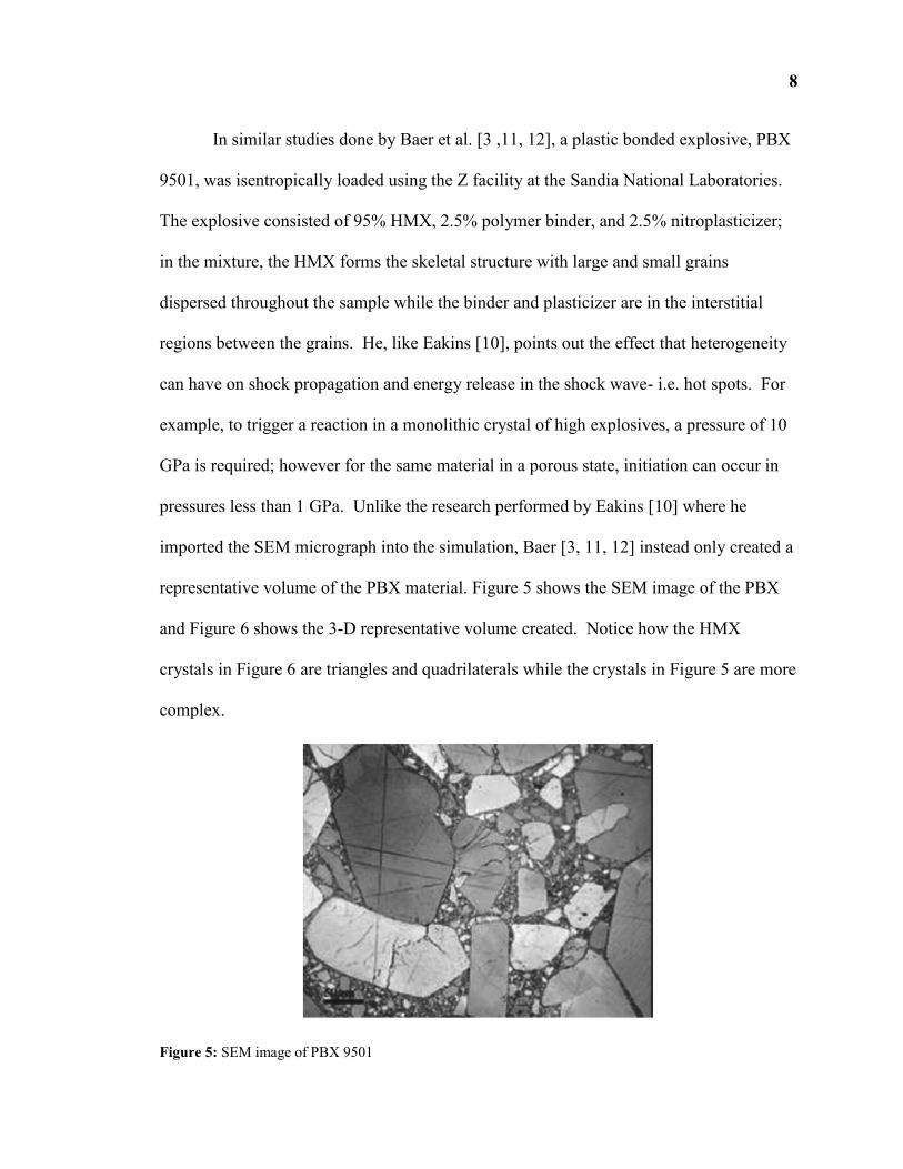
In similar studies done by Baer et al. [3 ,11, 12], a plastic bonded explosive, PBX

9501, was isentropically loaded using the Z facility at the Sandia National Laboratories.

The explosive consisted of 95% HMX, 2.5% polymer binder, and 2.5% nitroplasticizer;

in the mixture, the HMX forms the skeletal structure with large and small grains

dispersed throughout the sample while the binder and plasticizer are in the interstitial

regions between the grains. He, like Eakins [10], points out the effect that heterogeneity

can have on shock propagation and energy release in the shock wave- i.e. hot spots. For

example, to trigger a reaction in a monolithic crystal of high explosives, a pressure of 10

GPa is required; however for the same material in a porous state, initiation can occur in

pressures less than 1 GPa. Unlike the research performed by Eakins [10] where he

imported the SEM micrograph into the simulation, Baer [3, 11, 12] instead only created a

representative volume of the PBX material. Figure 5 shows the SEM image of the PBX

and Figure 6 shows the 3-D representative volume created. Notice how the HMX

crystals in Figure 6 are triangles and quadrilaterals while the crystals in Figure 5 are more

complex.

Figure 5: SEM image of PBX 9501

9

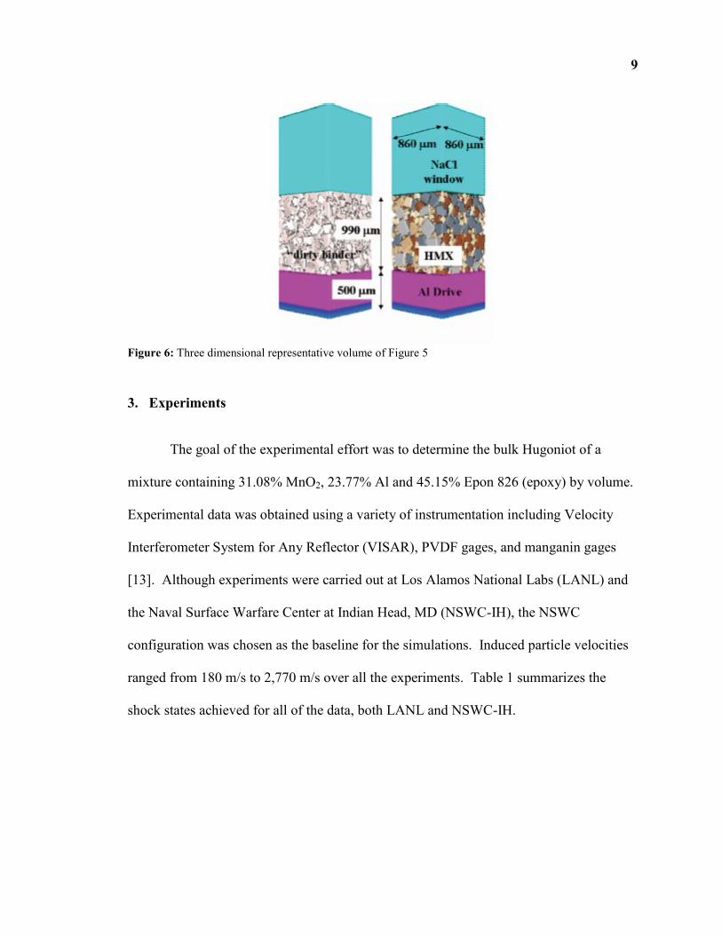
Figure 6: Three dimensional representative volume of Figure 5

3. Experiments

The goal of the experimental effort was to determine the bulk Hugoniot of a

mixture containing 31.08% MnO2, 23.77% Al and 45.15% Epon 826 (epoxy) by volume.

Experimental data was obtained using a variety of instrumentation including Velocity

Interferometer System for Any Reflector (VISAR), PVDF gages, and manganin gages

[13]. Although experiments were carried out at Los Alamos National Labs (LANL) and

the Naval Surface Warfare Center at Indian Head, MD (NSWC-IH), the NSWC

configuration was chosen as the baseline for the simulations. Induced particle velocities

ranged from 180 m/s to 2,770 m/s over all the experiments. Table 1 summarizes the

shock states achieved for all of the data, both LANL and NSWC-IH.

10

1Table 1: Shock states achieved during experiments

Exp. No. Us

(km/s)

Us – Tilt Corrected

(km/s)

Up

(km/s)

P

(GPa)

JJH14 4.16 ± 0.60 4.28 ± 0.50 0.94 ± 0.34 10.5 ± 3.9

JJH15 5.30 ± 0.38 5.36 ± 0.31 1.36 ± 0.25 18.9 ± 3.7

JJH16 4.85 ± 0.22 4.90 ± 0.08 1.42 ± 0.39 18.1 ± 4.9

JJH28 2.90 ± 0.15 0.18 ± 0.03 1.4 ± 0.2

JJH28 PVDF 2.85 0.17 1.3 ± 0.1

JJH29 3.61 ± 0.32 0.35 ± 0.07 3.3 ± 0.1

JJH30 3.30 ± 0.07 0.63 ± 0.02 5.4 ± 0.2

JJH54 4.84 ± 0.34 4.91 ± 0.27 1.38 ± 0.06 17.6 ± 1.2

JJH55 5.02 ± 0.44 5.09 ± 0.32 1.36 ± 0.06 18.0 ± 1.4

JJH56 4.07 ± 0.24 4.16 ± 0.11 0.81 ± 0.03 8.8 ± 0.4

JJH57 4.24 ± 0.26 4.30 ± 0.18 0.81 ± 0.03 9.0 ± 0.5

JJH58 5.37 ± 0.18 5.38 ± 0.16 1.76 ± 0.09 24.5 ± 1.4

JJH59 5.08 ± 0.24 5.15 ± 0.12 1.78 ± 0.09 23.9 ± 1.3

JJH60 4.80 ± 0.22 4.86 ± 0.10 1.29 ± 0.19 16.2 ± 2.4

JJH61 4.78 ± 0.25 4.86 ± 0.13 1.12 ± 0.19 14.2 ± 2.4

JJH62 4.45 ± 0.31 4.46 ± 0.29 1.33 ± 0.12 15.4 ± 1.7

JJH63 4.16 ± 0.32 4.20 ± 0.28 1.36 ± 0.12 14.8 ± 1.6

JJH64 3.96 ± 0.26 3.99 ± 0.22 0.90 ± 0.13 9.3 ± 1.4

JJH65 3.98 ± 0.37 4.00 ± 0.36 0.91 ± 0.13 9.3 ± 1.6

JJH31 3.12 ± 0.22 0.57 ± 0.04 4.6 ± 0.4

JJH32 2.98 ± 0.15 0.41 ± 0.03 3.2 ± 0.3

2S-318 5.578 1.365 19.87

2S-333 4.978 2.269 11.95

2S-336 5.333 2.770 16.31

JJH120 3.64 ± 0.13 0.32 ± 0.06 3.0 ± 0.6

JJH121 – man. 3.88 0.48 4.8 ± 0.1 (I)

3.4 ± 0.7 (T)

JJH121 PVDF 3.88 0.41 4.2 ± 0.2 (I)

JJH122 – man. 3.93 0.48 4.9 ± 0.2 (I)

4.1 ± 1.8 (T)

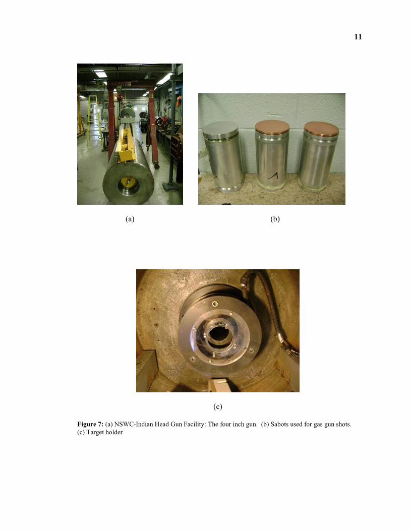
The experiments performed at the NSWC- Indian Head were performed on their

four-inch one stage light gas gun. Images of the facility and the sabots used are presented

in Figure 7.

1 Distribution A: Approved for public release 96 ABW/PA 09-03-08-385

11

(a) (b)

(c)

Figure 7: (a) NSWC-Indian Head Gun Facility: The four inch gun. (b) Sabots used for gas gun shots.

(c) Target holder

12

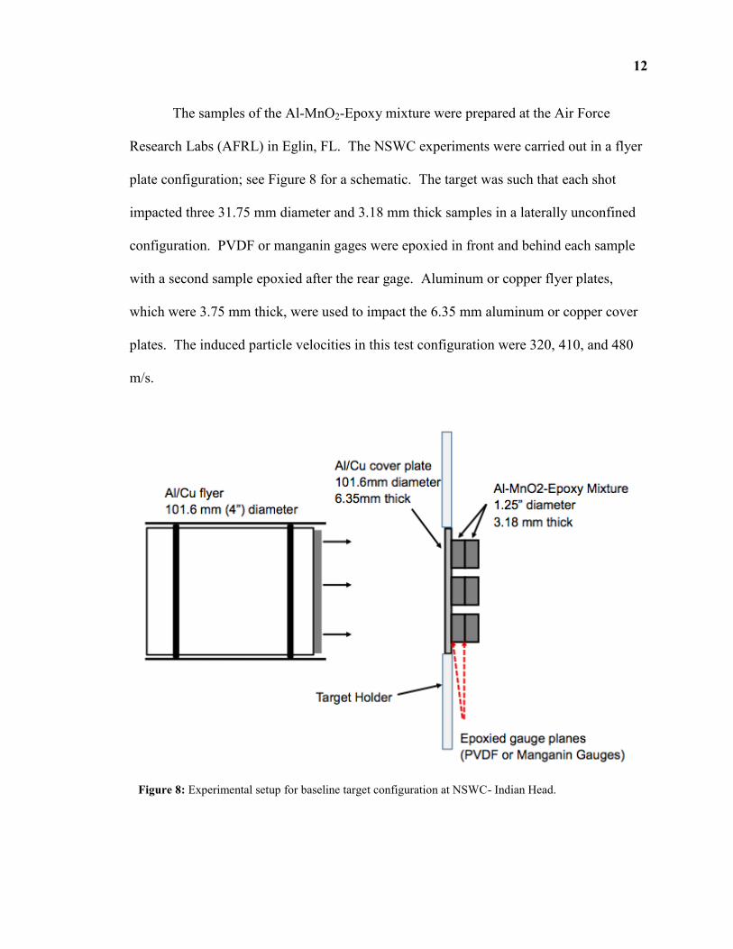
The samples of the Al-MnO2-Epoxy mixture were prepared at the Air Force

Research Labs (AFRL) in Eglin, FL. The NSWC experiments were carried out in a flyer

plate configuration; see Figure 8 for a schematic. The target was such that each shot

impacted three 31.75 mm diameter and 3.18 mm thick samples in a laterally unconfined

configuration. PVDF or manganin gages were epoxied in front and behind each sample

with a second sample epoxied after the rear gage. Aluminum or copper flyer plates,

which were 3.75 mm thick, were used to impact the 6.35 mm aluminum or copper cover

plates. The induced particle velocities in this test configuration were 320, 410, and 480

m/s.

Figure 8: Experimental setup for baseline target configuration at NSWC- Indian Head.

13

4. Computer Simulations

4.1. Geometry

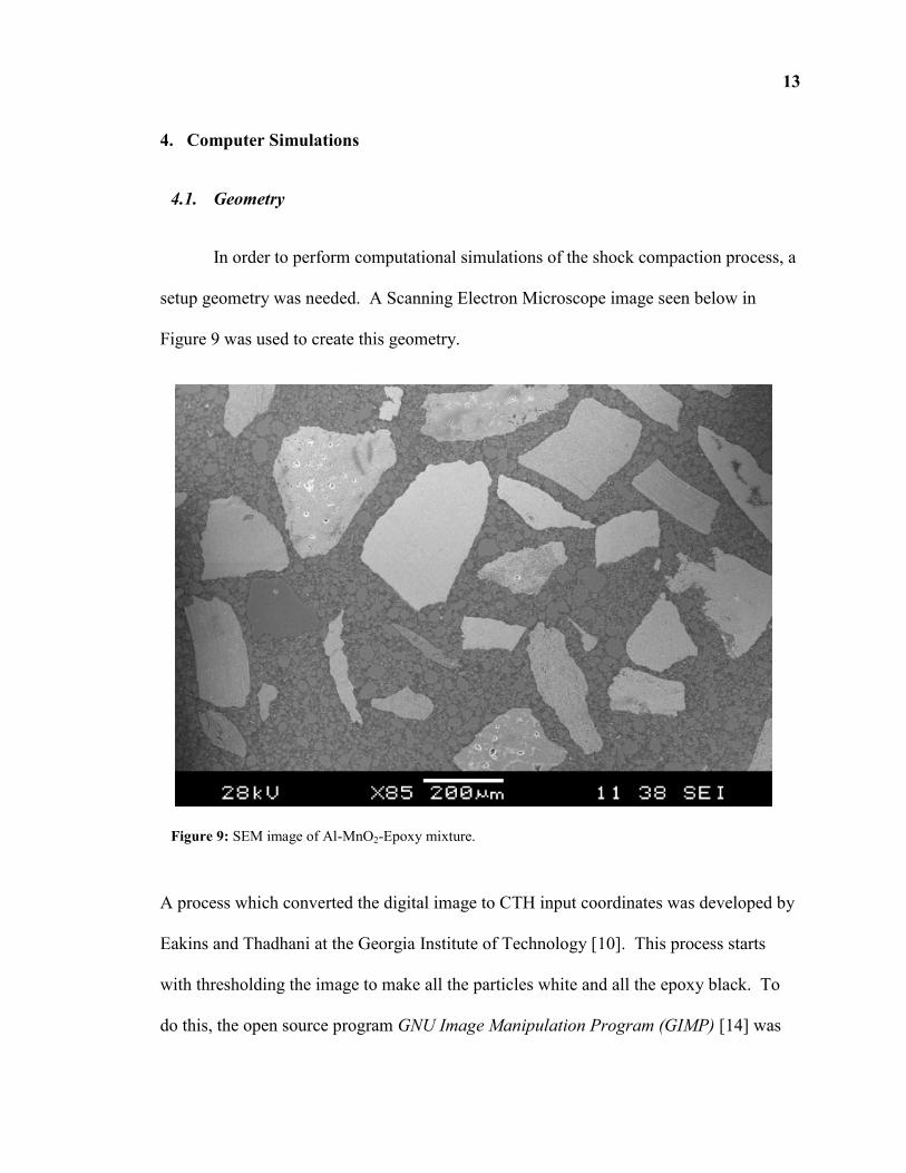
In order to perform computational simulations of the shock compaction process, a

setup geometry was needed. A Scanning Electron Microscope image seen below in

Figure 9 was used to create this geometry.

A process which converted the digital image to CTH input coordinates was developed by

Eakins and Thadhani at the Georgia Institute of Technology [10]. This process starts

with thresholding the image to make all the particles white and all the epoxy black. To

do this, the open source program GNU Image Manipulation Program (GIMP) [14] was

Figure 9: SEM image of Al-MnO2-Epoxy mixture.

14

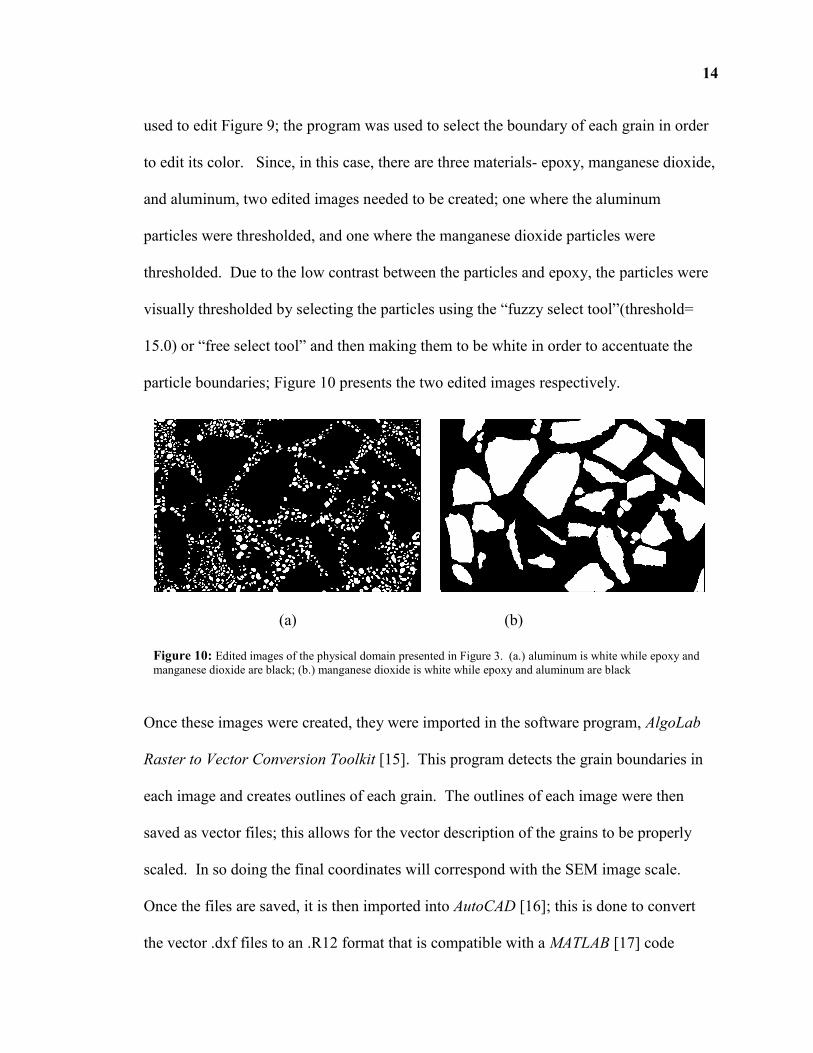
used to edit Figure 9; the program was used to select the boundary of each grain in order

to edit its color. Since, in this case, there are three materials- epoxy, manganese dioxide,

and aluminum, two edited images needed to be created; one where the aluminum

particles were thresholded, and one where the manganese dioxide particles were

thresholded. Due to the low contrast between the particles and epoxy, the particles were

visually thresholded by selecting the particles using the “fuzzy select tool”(threshold=

15.0) or “free select tool” and then making them to be white in order to accentuate the

particle boundaries; Figure 10 presents the two edited images respectively.

Once these images were created, they were imported in the software program, AlgoLab

Raster to Vector Conversion Toolkit [15]. This program detects the grain boundaries in

each image and creates outlines of each grain. The outlines of each image were then

saved as vector files; this allows for the vector description of the grains to be properly

scaled. In so doing the final coordinates will correspond with the SEM image scale.

Once the files are saved, it is then imported into AutoCAD [16]; this is done to convert

the vector .dxf files to an .R12 format that is compatible with a MATLAB [17] code

(a) (b)

Figure 10: Edited images of the physical domain presented in Figure 3. (a.) aluminum is white while epoxy and

manganese dioxide are black; (b.) manganese dioxide is white while epoxy and aluminum are black

15

developed by Georgia Tech. This code converts the .R12 file into CTH coordinates that

can be directly inserted in the CTH setup file.

In order to reproduce the full experimental geometry in CTH, a larger domain was

required than was provided by the SEM image. This was accomplished by mirroring the

original image twice in the longitudinal direction. Due to the resolution of the SEM

images as well as the post processing, not all of the aluminum particles are resolved via

our image conversion process. Therefore, in order to match the volume fraction of the

computational work with the experimentally measure volume fraction, aluminum spheres

were randomly inserted into the domain; MnO2 particles were also removed for the same

reason.

Once this was done, the bulk density within CTH (2.70 g/cc) still did not match

the density measured in the experiments (2.59-2.61 g/cc). Upon closer inspection of the

SEM images, it was noticed that the MnO2 particles were not fully consolidated but

rather porous. The density of the MnO2 in CTH was then lowered from 5.026 g/cc to

4.55 g/cc in order to match the bulk densities and account for the porous nature of the

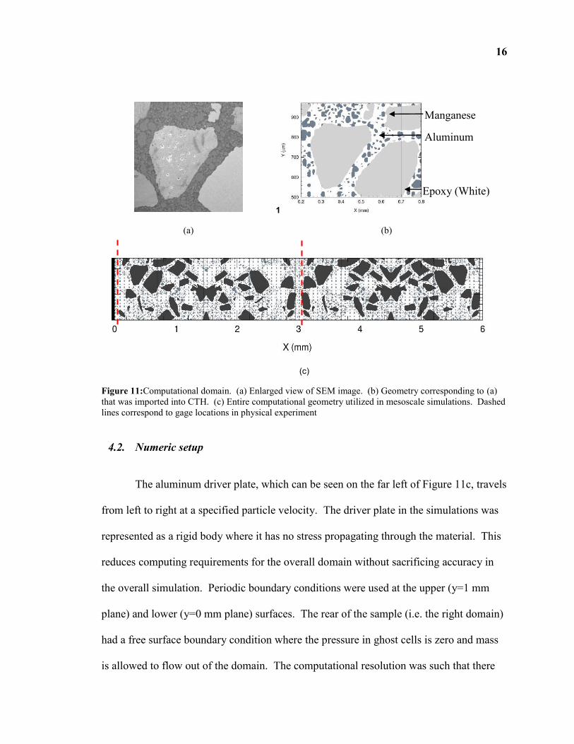
MnO2. The resulting computational domain from CTH is shown below in Figure 11c

while the corresponding views of the SEM image and the computation geometry can be

seen in Figure 11a and Figure 11b.

16

(a)

1

(b)

(c)

Figure 11:Computational domain. (a) Enlarged view of SEM image. (b) Geometry corresponding to (a)

that was imported into CTH. (c) Entire computational geometry utilized in mesoscale simulations. Dashed

lines correspond to gage locations in physical experiment

4.2. Numeric setup

The aluminum driver plate, which can be seen on the far left of Figure 11c, travels

from left to right at a specified particle velocity. The driver plate in the simulations was

represented as a rigid body where it has no stress propagating through the material. This

reduces computing requirements for the overall domain without sacrificing accuracy in

the overall simulation. Periodic boundary conditions were used at the upper (y=1 mm

plane) and lower (y=0 mm plane) surfaces. The rear of the sample (i.e. the right domain)

had a free surface boundary condition where the pressure in ghost cells is zero and mass

is allowed to flow out of the domain. The computational resolution was such that there

Manganese

Dioxide Aluminum

Epoxy (White)

17

was a minimum of eleven cells across the smallest grain; this equals 3300 nodes in the x-

direction (0.6005 cm), 550 nodes in the y-direction (0.1 cm) and 1.82 μm/cell.

4.3. Material Properties

The following describes the constitutive models for each material utilized in these

calculations; Table 2 summarizes their respective material properties. It is important to

keep in mind that the mesoscale configuration means each constituent is modeled as a

fully consolidated material. No mixtures models are necessary because the simulation is

resolving each grain.

4.3.1. Aluminum

Each material was assigned an appropriate built in equation of state and strength

model. One of the great advantages of mesoscale simulations, over bulk simulations, is

that mixture models are not necessary to describe the bulk material behaviors. The bulk

behavior is resolved by integrating the over the entire domain, which consists of a

collection of grains. The simulation, which resolves each material separately, assigns the

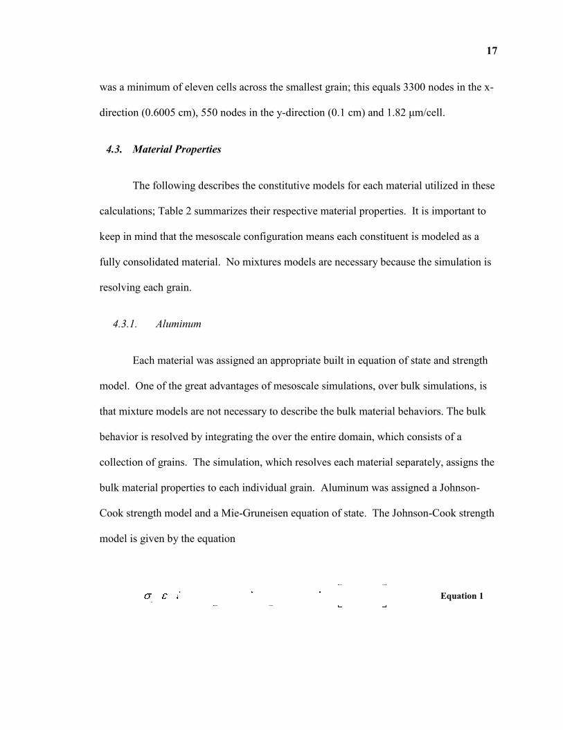
bulk material properties to each individual grain. Aluminum was assigned a Johnson-

Cook strength model and a Mie-Gruneisen equation of state. The Johnson-Cook strength

model is given by the equation

*, , 1 ln 1mn

y P P P PT A B C T Equation 1

18

where p is the equivalent plastic strain, P is the plastic strain-rate, and A, B, C, n, and m

are material constants. While the normalized plastic strain-rate and temperature in

Equation 1 are defined as

0

* PP

P

Equation 2

0*

0

:m

T TT

T T Equation 3

where 0P is a plastic strain-rate defined by the user, T0 is a reference temperature, and

Tm is a reference melt temperature. The Johnson-Cook strength model was chosen

because it captures strain-rate dependent behavior; it is known that materials can work

harden while under strain [18]. This is needed for the multiscale work described in

Section 5. The Johnson-Cook has been previously implemented within CTH and has

numerous materials built into the model, including aluminum.

The Mie-Gruneisen equation of state is based on the Mie-Gruneisen

approximation given by 1 /P E where Γ is the Gruneisen parameter and is

only a function of density [19]. This leads to a linear relationship between pressure and

density given by

0 0, H HP E P E E Equation 4

where PR and ER are a reference pressure and energy generally given by the Hugoniot.

To find temperature, it is assumed that the constant-volume specific heat /v vC E T

is constant which leads to

, H v HE T E C T T. Equation 5

19

4.3.2. Manganese Dioxide

The manganese dioxide was assigned a Johnson-Holmquist II (JH-2) ceramic

model [20]; as implemented in CTH, this functions both as an equation of state and a

strength model. The reason the JH-2 model was selected for this study is because it

models the strain softening behavior that ceramics exhibit in experiments. The JH-2

model computes the yield surface depending on a scalar damage parameter. Figure 12

presents strength curves for a ceramic material in the JH-2 model. One can see that

initially the material has a specific strength curve; but as the damage accumulates, the

strength curve is reduced.

In order to capture this behavior a damage parameter, D, is introduced. This parameter is

bound between zero and one (0≤D≤1) and is used to calculate the normalized flow stress

as follows:

* * * *i i fD Equation 6

Figure 12: Strength in the JH-2 model [20].

20

where *i and *

f are the intact and fractured normalized flow stresses respectively. The

normalized flow stresses * * *, ,i f are found from the general form * / HEL

where σ is the plastic flow stress and σHEL is the Hugoniot Elastic Limit (HEL). The

normalized intact and fractured stress are found from

* * * 1 lnN

i A P T C Equation 7

* * 1 lnM

f B P C Equation 8

The material constants in these equations are A, B, C, M, N, and SFMAX; note that

SFMAX is a parameter that can limit the fracture strength by *f SFMAX in order to

provide flexibility in defining the fracture strength. The normalized pressure P* is found

from * / HELP P P where P is the pressure and PHEL is the pressure at the HEL. The

normalized maximum tensile hydrostatic pressure is found from * / HELT T P , where T is

the maximum tensile hydrostatic pressure the material can withstand.

The damage parameter is expressed as

P

Pf

D Equation 9

where P is the plastic strain during a cycle of integration and

Pf is the plastic strain to

fracture under a constant pressure, P; the expression for this is

2* *1

DPf D P T Equation 10

where D1 and D2 are constants and P* and T

* are as defined previously.

21

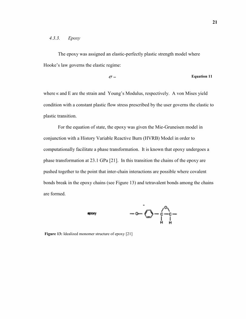
4.3.3. Epoxy

The epoxy was assigned an elastic-perfectly plastic strength model where

Hooke‟s law governs the elastic regime:

E Equation 11

where and E are the strain and Young‟s Modulus, respectively. A von Mises yield

condition with a constant plastic flow stress prescribed by the user governs the elastic to

plastic transition.

For the equation of state, the epoxy was given the Mie-Gruneisen model in

conjunction with a History Variable Reactive Burn (HVRB) Model in order to

computationally facilitate a phase transformation. It is known that epoxy undergoes a

phase transformation at 23.1 GPa [21]. In this transition the chains of the epoxy are

pushed together to the point that inter-chain interactions are possible where covalent

bonds break in the epoxy chains (see Figure 13) and tetravalent bonds among the chains

are formed.

Figure 13: Idealized monomer structure of epoxy [21]

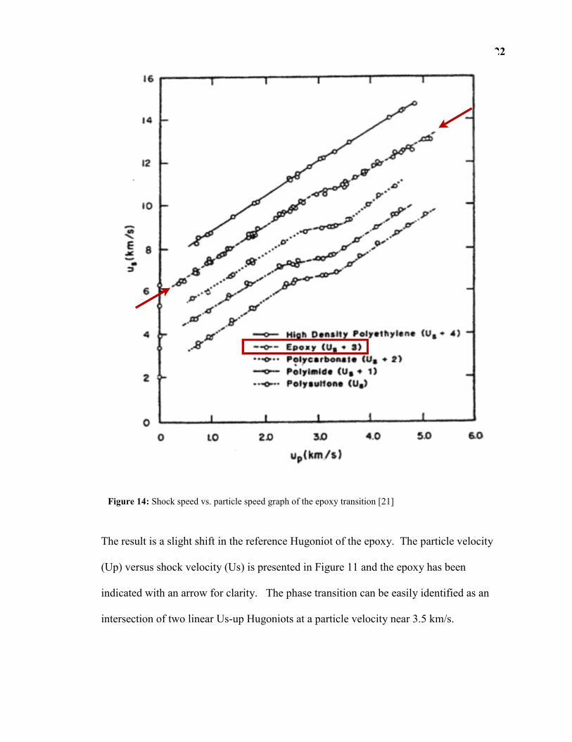
22

The result is a slight shift in the reference Hugoniot of the epoxy. The particle velocity

(Up) versus shock velocity (Us) is presented in Figure 11 and the epoxy has been

indicated with an arrow for clarity. The phase transition can be easily identified as an

intersection of two linear Us-up Hugoniots at a particle velocity near 3.5 km/s.

Figure 14: Shock speed vs. particle speed graph of the epoxy transition [21]

23

The HVRB model was used as a trigger in the hydro-code to initiate the phase

transition. The HVRB model is a pressure-dependent continuum reaction model in which

extent of reaction, λ, is integrated over time at a given mass point. The model has the

following form:

1 1

XM

X Equation 12

00

1 ti

R

P Pdt

P Equation 13

where X, PR and z are reaction rate parameters, and Pi is the threshold pressure for

reaction. Although the HVRB model is typically used to describe reaction rates for

explosives, where solid reactants equation of state is mixed with gaseous products

equation of state, in this case it was used to transition from a solid (phase I) to a solid

(phase II) equation of state. Thus default reaction parameters were mostly used to

simplify the transition. The parameters PR and z determine the pressure dependence of

time and distance to reaction and are usually fit to wedge test data. The exponent M

controls the time delay to pressure build up behind the shock front and X determines the

rate at which the reaction proceeds to completion; τ0 is used to make dimensionless

and is not an independent constant. Table 3 lists the input HVRB parameters used in this

study. The use of an HVRB model allowed for the use of two Mie-Gruneisen equations

of state for the epoxy; one for phase I when the local pressure in the epoxy is below the

23.1 GPa reaction threshold, and one for the transition phase when the local pressure is

above the threshold. A second set of simulations were performed in which the epoxy was

assigned a Mie-Gruneisen equation of state which corresponded to pure phase II epoxy;

24

this was done in order to establish the full transition compaction behavior. This is of

especial interest in a mesoscale configuration where the localized stresses can vary thus

either aiding or delaying a pressure driven phase transition mechanism. The parameter

constants associated with each phase of the epoxy is listed in Table 2.

Table 2: Equation of State and Constitutive Material Parameters

Parameter MnO2†

[22,23,24]

Al

[25,26]

Epoxy††

Phase I [22,27, 28]

Epoxy

Transition Phase

[22,27,28]

Epoxy

Phase II [22,27,28]

Density, [g/cm3] 4.55 2.703 1.19 1.19 1.19

Zero stress shock speed, C0 [km/s] 3.632 5.288 2.67 7.88 2.88

Hugoniot slope, s 1.52 1.3756 1.55 0.01 1.35

Grüneisen coefficient, G=V( P/ E)V 1.25 2.14 2.18 2.18 2.18

Specific heat, CV [J/(g-K)] 0.67 0.885 2.1 2.1 2.1

Bulk Dynamic yield strength, Y [GPa] 7.5 0.29 0.069 0.069 0.069

Poisson’s ratio, 0.28 0.32 0.36 0.36 0.36

Bulk Modulus, K [GPa] 34.4 75.5 8.48 73.9 9.87

Fracture strength, s [GPa] N/A 60 60 60 60

† Johnson-Holmquist II Strength [20]

†† Epon 828 Data

Table 3: History Variable Reactive Burn (HVRB) Parameters

Parameter Value Parameter Value

Reaction rate, X [unit less] 1.0† Time delay, M [unit less] 1.5

†

Pressure threshold, Pi [GPa] 23.1 Reaction rate, PR [GPa] 5.0†

Pressure dependence, z [unit less] 3.0†

† Default [29]

4.4. Results

4.4.1. Material Movement

Material plots were generated in order to explore the grain-on-grain and grain-

binder interactions within the mixture matrix. Figure 15 presents the two-dimensional

stress response of the material where the contours represent pressure. The contours

25

demonstrate that the epoxy undergoes larger deformation than does the more rigid MnO2

or Al; thus the load is carried by the epoxy. The result is a spatially and temporally

varying stress state behind the initial compaction wave. The post processor indicates

stresses below the legend as white and clips all the stresses above the legend as black.

Thus, in Figure 15, a spatially large low-pressure precursor stress can be seen as the all-

white portion located ahead of the shock front. For these relatively small grains the

shock compaction of the entire computational domain takes less than 2 s.

Figure 15: Compaction response of the Al-MnO2-Epoxy mixture at a flyer plate velocity of Up= 480 m/s.

4.4.2. Conduction

One area of interest is the conduction of heat through each grain. Will there be

significant heat conduction through any grain when dealing with the micron timescale?

What is the characteristic length associated with the adiabatic assumption when applied

to a heterogeneous material? Simple calculations were made in order to roughly estimate

a) t= 0.792 μs

b) t= 1.29 μs

26

the thermal diffusion distance. As suggested by Meyers [19], the characteristic

dimensions of heat diffusion distance can be estimated by

2d t , Equation 14

where d is the distance heat is conducted, is the thermal diffusivity, and t is the time

under strain; for aluminum, is about 0.65cm2/s from 300 K to 700 K [30]. The time

under strain is estimated by dividing the grain radius by the shock speed. To see what the

largest depth of conduction possible, the smallest shock speed of 2.9 km/s was used

(6

3

10 10

2.9 10 /

x mt

x m s) to get a time of 3.448 ps. The resulting distance of conduction is

0.947d maround a 20 m diameter aluminum particle. Thus the diffusion diameter is

10 times smaller than the grain diameter. As a result it was concluded that the adiabatic

assumption is still valid for this mixture. However, this does not account for possible heat

transfer from the epoxy to the aluminum particle and including a conduction model in the

simulations will be considered in future work.

4.4.3. Bulk Response

The bulk Hugoniot response was obtained by locating the bulk compaction wave

front at various snapshots in time during the simulation. For each snapshot, the

longitudinal stress was averaged in the lateral direction in order to produce a single

instantaneous bulk wave profile as it traversed the domain. The compaction wave

location was assigned to the half-height of the transmitted longitudinal stress wave front.

By knowing the location of the bulk compaction wave and the time at which the snapshot

was obtained, the compaction wave speed could be calculated. Figure 16 presents the

27

averaged bulk compaction wave speed through the sample, as a function of longitudinal

position. Each trace represents a different flyer plate particle velocity. Figure 16

indicates that the bulk compaction wave speed is fairly constant as it traverses the

sample. From these results it appears that the wave speed reaches steady state at

approximately 3 mm, which corresponds to roughly 12 MnO2 grain characteristic lengths.

From this data the compaction-particle velocity relationship can be obtained and

projected onto density-stress space via the Rankine-Hugoniot relations.

Figure 17 presents a comparison of the experimental and simulated bulk

compaction response. The experimental results were fit to a linear Us-Up Hugoniot and

projected onto density-stress space via the Rankine-Hugoniot equations

0 s pP U U . Equation 15

Figure 16: Comparison of the averaged wave speeds at various positions in the sample.

28

0

1 0

1 1 11

s

c

S SU Equation 16

The Us-Up experimental data clearly indicates a change in slope near particle

velocities of 0.80 km/s. As discussed in Section 4.3.3, it is well documented that epoxy

undergoes a phase transition at these conditions [21]. Thus the discontinuity in the Us-

Up data is associated with the epoxy phase transition. At low stress levels, the

experimental data and simulated response agree very well, while at high stress levels near

25 GPa, the computational data splits the two experimental points. One must assume that

by the time the mixture reaches these pressures, nearly all epoxy should be in the third

phase. However, in the transition region, the experimental data exhibits substantial

scatter, which may be due to variations in the mixture. The sensitivity of the transition

region is unknown and could be explored in future work.

29

(a)

(b)

Figure 17: Bulk compaction response: experiment and simulation. Experimental data is fit to linear Us-Up

and indicated by the solid black line in the figure. Dashed line is for the comparison of slopes between

phase I and phase II of the epoxy

30

5. Investigation of the effect of multi-scale grain sizes

5.1. Geometry

Initially, a novel procedure was attempted to investigate the effects of grain size

in mesoscale simulations with regards to hot spot formations. To reduce the computing

requirement of computationally resolving nano-sized particles in a millimeter-size

computational domain, a sub-grid area of investigation was selected from the mesoscale

simulation. The area selected is illustrated in the upper portion of Figure 18; this area

was selected due to the formation of a hot-spot. The shock appears to extrude the

aluminum-binder material through the channel created by two large MnO2 particles

thereby generating very high localized shear and deformation, which results in a local hot

spot.

Figure 18: Area of investigation for novel attempt to simulate nano particles (nano particles are in this

image, but are too small to appear on this large plot domain).

31

To set up the sub-grid simulations, the full domain setup discussed previously in Section

4.1 was re-computed with a box of tracers inserted in the area of interest; this was done to

gather velocity data, which can then be applied as boundary conditions to the sub-grid

model. Afterwards, the computational domain was cropped to the area shown above in

the lower area of Figure 18. Then, the data gathered from the tracers in the full domain

mesoscale simulation was used to drive a rigid plate, initially on the boundary of the

tracers, through the channel in between the right and left MnO2 particles. In addition to

the driver plate, the left MnO2 particle was also given a velocity. To compare the two

domains and insure the transition from the mesoscale domain to the sub-grid domain

faithfully conserves energy, the kinetic energy obtained from the tracers was compared

between the full and the cut down domain. Once the energy differences were

minimized, nano-sized particles were inserted into the trimmed domain. The original

mass fraction of the aluminum was maintained throughout the investigation. However,

due to the computing requirement to resolve nano-sized aluminum particles this process

had to be abandoned. This was essentially due to the fact that at these small scales it is

impossible to capture both the characteristic dimension of the particles and a

representative volume.

Developing sub-grid representations in the manner described above was fraught

with difficulties. The difficulties associated with resolving, what is essentially a non

rectangular domain (the channel illustrated in Figure 18) with a rectangular Cartesian

mesh seemed unnecessary. In addition, a small velocity gradient at the boundary was

implemented which created step-wise discontinuous deformation. Finally, the

morphology and roughness associated with the MnO2 at the sub-grid scale was near the

32

limitations of the SEM image. Thus enforcing these geometries at the sub-grid seemed

unnecessary. Therefore this methodology (extracting a geometry from the mesoscale and

inserting into the sub-scale) was abandoned and an alternative procedure was pursued.

Instead of using a portion of the geometry from the SEM image, the loading

characteristics were applied to a representative geometry constructed from simple shapes.

However, the boundary velocities extracted from the bulk mesoscale simulations were

still used to establish the boundary conditions applied to a sub-grid representative

volume. This resulted in a representative volume domain that could resolve nanometer

particles and voids in a more computationally tractable geometry. The essential features

of the flow were retained, namely extruding the binder-aluminum mixture between two

large, relatively high-impedance, ceramic grains

Figure 19 presents the representative volume created in this effort. In the sub-grid

domain, there are two MnO2 grains (dark grey), one on the top and one on the bottom. In

between these two MnO2 grains are epoxy (light grey) and aluminum particles (grey) in

which the size will be varied from the micron-scale down to the nano-scale. During the

simulation the MnO2 grains move towards each other at a specified initial velocity,

effectively crushing and shearing the aluminum and epoxy mixture. The aluminum

particles were intentionally arranged in order to simulate interesting grain scale dynamics

observed from previous mesoscale simulations [31, 32]. Specifically these include the

formation of dynamic stress bridges, which is facilitated by grains loosely arranged in the

direction of the shock. This effect will be enhanced given that the grain arrangement is

percolated through the domain. The novel idea pursued here is using boundary conditions

33

extracted from the bulk mesoscale simulations in order to drive a subscale simulation

exploring the role of nano-particles and strain hardening constitutive relations.

Figure 19: Computational domain utilized in the multiscale investigation

The scale of the computational domain, as presented in Figure 19, was varied in

order to investigate a large range of particle sizes within the test matrix and the effect of

varying the length scale while enforcing a strain-rate constitutive model. In addition, the

thickness of the alumina (Al2O3) coating was varied, which effectively changes the

overall density and yield strength of the aluminum particles. The thickness of the coating

was varied between 0 and 3 nm [33]. Removing the alumina coating at the nano scale

was done to more faithfully compare the effect of particle size variations from millimeter

to nanometer scales without the complications associated with simultaneously changing

the density and bulk mixture yield strength.

34

5.2. Numeric Setup

The MnO2 particles on the top and bottom of the domain both compressed the

epoxy and aluminum particles at speeds of -450 m/s and 450m/s respectively; these

velocities were extracted and representative of the average particle velocities observed in

the MnO2 during the sub-grid compaction event [31]. The top and bottom boundary

conditions are such that the sound speed is transmitted (semi-infinite solid), while the

MnO2 simultaneously continues to flow into the computational domain from the top and

bottom as the simulation progresses. This saved the computational expense associated

resolving large volumes of MnO2. Symmetry was imposed along the x=0 axis (the

domain is mirrored about x=0). The right boundary imposed zero pressure and mass

removal in the ghost cells; no mass can enter along the boundary, but mass can exit. Due

to the symmetry of the domain and the boundary conditions, a large shear gradient was

established in the epoxy/aluminum mixture as the mixture is extruded to the right.

5.3. Material Properties

The material properties used in this process were all the same as from Section 4.3.

In addition, aluminum oxide was used as a coating around the pure aluminum alloy. A

Johnson-Cook model and a Mie-Gruneisen equation of state were used to model the

alumina. Because these are mesoscale computations, various nanoscale particle effects,

such as phonon scattering at the interfaces, are not accounted for. The material properties

can be seen in Table 4. The fracture strength was turned on for the multiscale

investigation. Previously the fracture strength was effectively turned off by giving all

materials a fracture strength that was unattainable. The reason both the Johnson-Cook

35

and Johnson-Holmquist II models were chosen in Section 4.3 was to incorporate strain-

rate dependent behavior in the simulations. If this was not done and only elastic-

perfectly plastic models were used for each material, the results would scale exactly with

the domain size.

Table 4: Equation of State and Constitutive Material Parameters II

Parameter MnO2

†

[22,23,24]

Al

[25,26]

Epoxy††

Phase I

[22,27,28]

Epoxy Transition

Phase [22,27,28]

Epoxy Phase

II [22,27,28]

Al2O3

[22,34]

Density, [g/cm3] 4.55 2.703 1.19 1.19 1.19 3.69

Zero stress shock speed, C0 [km/s]

3.632 5.288 2.67 7.88 2.88 0.987

Hugoniot slope, s 1.52 1.3756 1.55 0.01 1.35 8.71

Grüneisen coefficient,

G=V( P/ E)V 1.25 2.14 2.18 2.18 2.18 2.14

Specific heat, CV [J/(g-K)]

0.67 0.885 2.1 2.1 2.1 0.885

Bulk Dynamic yield strength, Y [GPa] 7.5 0.29 0.069 0.069 0.069 15.4

Poisson’s ratio, 0.28 0.32 0.36 0.36 0.36 0.21

Bulk Modulus, K [GPa] 34.4 N/A 8.48 73.9 9.87 N/A

Fracture strength, s [GPa]

N/A 0.31 0.013 0.013 0.013 0.31

5.4. Results

Material plots were generated to explore the grain interactions within the domain

as well as identify regions that generate the highest temperature. Figure 20 presents an

example where the hotter areas are at the edges where the three large aluminum particles

are in contact and at the shear bands in the MnO2.

36

Figure 20: Temperature contour of aluminum particles with a 3nm alumina coating at 110ps (t/t0=0.44).

In addition, a plot was made with the maximum temperature within the entire

computational domain at each time step; see Figure 21. This method was chosen for

simplicity to check if there are any potential temperature changes in the hot regions as the

aluminum particle size is varied. The time has been normalized by the simulation time in

order to compare temperature profiles across a wide range of scales. As the particle size

was varied from milli-sized to nano-sized, the maximum temperatures reached are

slightly increased due to the strain hardening associated with higher local strain rates.

When the alumina coating was varied from 1 to 3 nm, the maximum temperature varied

to some extent, though no pattern of behavior can be conclusively detected.

37

Figure 21a: Maximum temperature achieved in the domain as a function of dimensionless time step.

(a) Variations in particle size.

Figure 21b: Maximum temperature achieved in the domain as a function of dimensionless time step.

(b) Variations in coating/adding voids

38

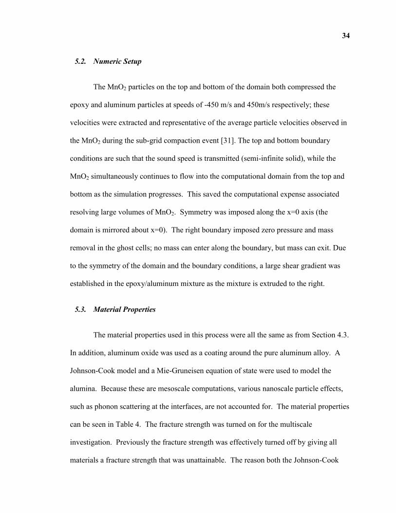
Lastly, a simulation was performed in which voids within the epoxy binder were

inserted into the domain to compare the effect of void collapse relative to strain

hardening. The geometry with the voids can be seen in Figure 22. It is well known that

voids cause hot spots to occur and can cause ignition in reactive materials [35]. The

reason for adding them in this case was to compare the effect on the temperature around

the voids with the effect of changing the particle size and alumina coating. As shown in

Figure 21b, the voids can increase the local temperature by nearly 600 K as opposed to

not having a void. This increase in temperature is sustained for nearly 30 ps, after which,

the temperature profile approaches the simulations without initial voids.

39

Figure 22: (Top) Geometry setup at 0.0 s with a 3 nm thick oxide layer and voids in the epoxy. (Bottom)

Temperature contour at 40.1 ps (t/t0=0.16); note hot spots corresponding to initial voids inserted in the

epoxy.

5.4.1. Conduction

Conduction calculations were also performed for the case of a 30 nm aluminum

grain in the same way as described for a 20 µm grain in Section 4.4.2. Assuming a same

shock speed of 2.9 km/s, the time under strain was found to be 5.17 ps. Using this value,

the distance of heat conducted was found to be 36.67 nm. Notice now that conduction is

now significant in the nanoscale case. Again, this will be a possible area of future

investigation where the simulations include model the effects of conduction.

6. Conclusions

The main goal of this thesis was to investigate the dynamic behavior of the Al-

MnO2-Epoxy mixture using experimental and computational data. In the first part, CTH

was used to model the shock compaction of the mixture at particle velocities ranging

from 180 m/s to 2770 m/s. The Johnson Cook and Johnson Holmquist strength models

40

were used for the aluminum and manganese dioxide respectively; these models are strain

rate dependent and will capture the strain hardening or softening the materials undertake

when they are compressed. For the epoxy, an elastic-perfectly plastic strength model was

used. The Mie-Gruneisen equation of state model was used for the aluminum and epoxy,

while the manganese dioxide equation of state was built in to the Johnson Holmquist

model. The computational results were then compared with experimental data gathered

at NSWC-IH and LANL. The two data sets were shown to be in agreement with one

another.

In the second part, a representative volume was created to perform a

computational multiscale investigation on the mixture. The aluminum grain size was

varied from 30 mm to 30 nm. Also, the aluminum oxide coating was varied, effectively

changing the overall strength of the grains. The results of these simulations were not as

conclusive as expected; only a slight trend could be seen as the grain sizes were varied

and no pattern was apparent when the aluminum oxide coating was varied.

41

7. References

[1] McGlaum, J.M., Thompson, S.L., and Elrick, M.G. Int. J. Impact Eng. 10, (1990), 351-360.

[2] Borg, J.P., and Vogler, T.J., Int. J. Solids Struct. 45, (2008), 1676–1696

[3] Baer, MR, Thermochimica Acta. 384, (2002), 351-367

[4] Benson, D.J. and Conley P., Modelling Simul. Mater. Sci. Eng. 7, (1999), 333-354

[5] Salas, Manuel D., “The Curious Events Leading to the Theory of Shock Waves.” Proceedings

of the 17th Shock Interaction Symposium, September 4-8 2006.

[6] Hayes, D.B., Introduction to stress wave phenomena. 1973, Lecture Notes.

[7] Millet, J.C.F., Deas, D, Bourne, N.K., Montgomery, S.T. “The deviatoric response of an

alumina filled epoxy composite during shock loading.” J. Appl. Phys. 102, 063518 (2007)

[8] Ferranti, L., Jordan, J.L., Dick, R.D., Thadhani, N.N. “ Shock Hugoniot behavior of particle

reinforced polymer composites.” In Shock Compression of Condensed Matter- 2007, edited by

M.D. Furnish, American Institute of Physics, 2007 p. 123-126

[9] Benson, David J, “Numerical Methods for Shocks in Solids.” Shock Wave Science and

Technology Reference Library. Springer Berlin Heidelberg. 2007, Pp. 275-320

[10] Eakins, D. and Thadhani, N.N., J. Appl. Phys. 101, 043508 (2007)

[11] Baer, M.R., Hall, C.A., Gustavsen, R.L., J. Appl. Phys. 101, 034906 (2007)

[12] Baer, Mel R., “Mesoscale Modeling of Shocks in Heterogeneous Reactive Materials.” Shock

Wave Science and Technology Reference Library. Springer Berlin Heidelberg. 2007, Pp. 321-

356

[13] Jordan, JL., Dattelbaum, DM, Sutherland, G, Richards, WD, . Sheffield, SA, and Dick J. of

App. Phys. (under preparation)

[14] GNU Image Manipulation Program

[15] Raster to Vector Conversion Toolkit, v. 2.97.62, Algolab Inc.

[16] AutoCAD 2008. Autodesk. San Rafael, CA. 2008

[17] MATLAB R2008a. The Math Works. Natick, MA. 2008

[18] Zerelli, F. J., and Armstrong, R. W., J. Appl. Phys, 61, 1816–1825 (1987).

[19] Meyers, Marc A., Dynamic Behavior of Materials. John Wiley and Sons, Inc., 1994

[20] Johnson and Holmquist, High-Pressure Science and Technology, 309, AIP Press, (1994)

981-4

[21] Carter, WJ and Marsh, SP. “Hugoniot Equation of State of Polymers.” LANL. LA-13006-

MS. 1995

[22] Marsh, S.P. LASL Shock Hugoniot Data (1980)

[23] Wang, Y, Zhang, J and Zhao, Y, Nano Letters 7, (2007), 3196-3199

[24] Swamy, V., Phys. Rev. B. 71, 184302 (2005)

[25] Steinberg, D.J., LLNL, UCRL-MA-106439, 1991

[26] Moshe, E., et. al., J. Appl. Phys. 83, 4004, 1998

[27] Austin, R, McDowell, D, and Benson, D. Modelling Simul. Mater. Sci. Eng. 14 (2006) 537-

561

[28] Richard C., Ting, R.Y., Audoly, C., “Development of 1-3 PZT-Polymer Composite for low

frequency acoustical applications.” Proceedings of the Ninth IEEE International Symposium

on Applications of Ferroelectrics, 1994.ISAF, August 7-10 1994. 291-294

[29] Kerley, GI “CTH Equation of state package: porosity and reactive burn models” Sandia

National Laboratories report SAND92-0553, 1992

[30] Jensen, J.E., Tuttle, W.A., et. al. BNL 10200-R 1980

42

[31] Fraser, A., Borg, J.P., Jordan J.L., Sutherland, G. “Exploring the micro-mechanical behavior

of Al-MnO2-Epoxy under shock loading while incorporating the epoxy phase transition”,

SEM Annual Conference & Exposition on Experimental & Applied Mechanics,

Albuquerque, NM, 2009

[32] Borg, JP and Vogler, TJ “Aspects of simulating the dynamic compaction of a granular

ceramic.” Modelling and Simulation in Materials Science and Engineering. 17, 045003,

(2009) pg 1-22

[33] Risha, G.A. et al. “Combustion of nano-aluminum and liquid water”, Proceedings of the

Combustion Institution 31 (2007) 2029-2036

[34] Alexander, William, Shackelford, James CRC Materials Science and Engineering

Handbook. CRC Press. 3rd

Edition, 2001.

[35] Bowden, F.P. and Yoffe, Y.D. Initiation and Growth of Explosions in Liquids and Solids.

Cambridge Univ. Press, New York, 1951

43

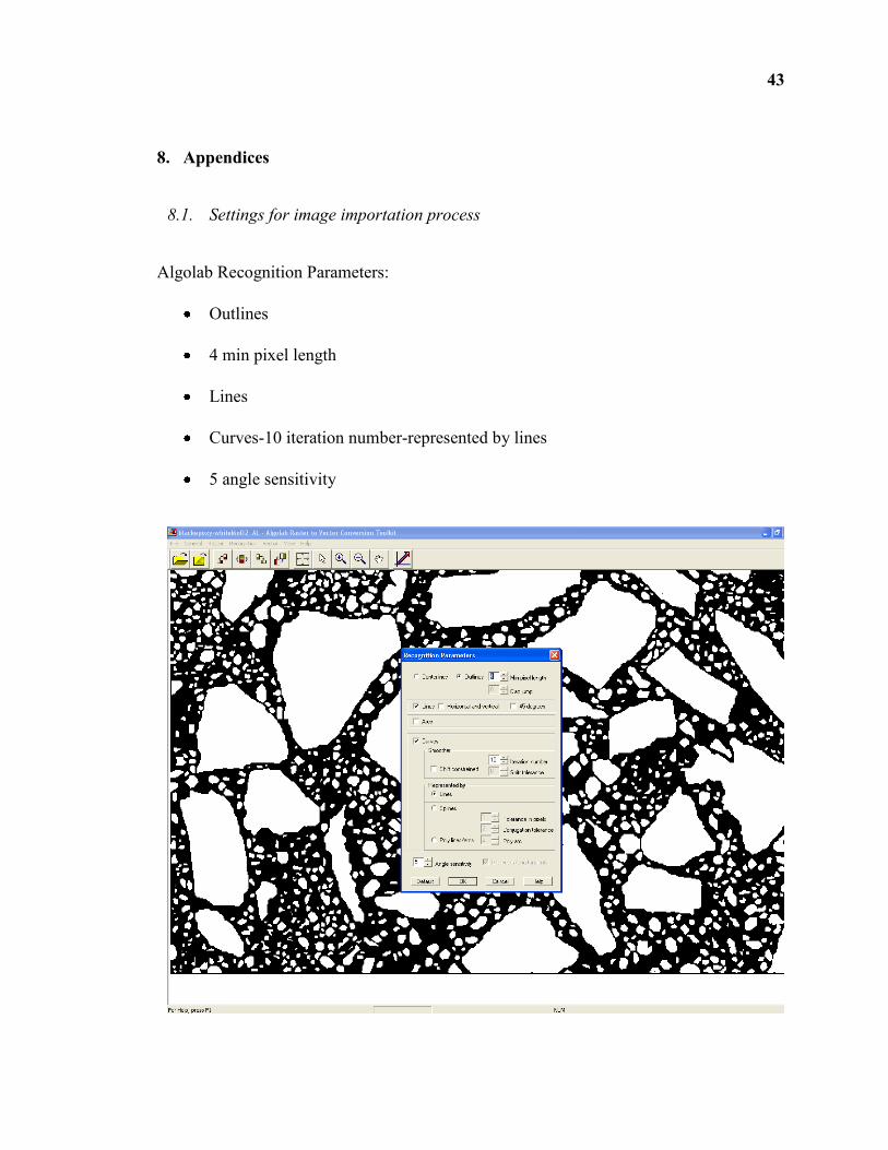
8. Appendices

8.1. Settings for image importation process

Algolab Recognition Parameters:

Outlines

4 min pixel length

Lines

Curves-10 iteration number-represented by lines

5 angle sensitivity

44

8.2. Calculations for conduction

For 20 µm grain:

Where d is the distance heat is conducted, is the thermal

diffusivity, and t is the time under strain

=0.65cm2/s for aluminum

2

Using the slowest shock speed leading to the largest conduction value

For 30 nm grain:

9

3

15 10

2.9 10 /

x mt

x m s

125.172 10t x s

63.667 10d x cm

36.67d nm

2 Jensen, J.E., Tuttle, W.A., et. al. BNL 10200-R 1980

45

8.3. Full domain material plots

(a)

(b)

(c)

(d)

Figure A.1: Pressure contour plots at selected snapshots in time

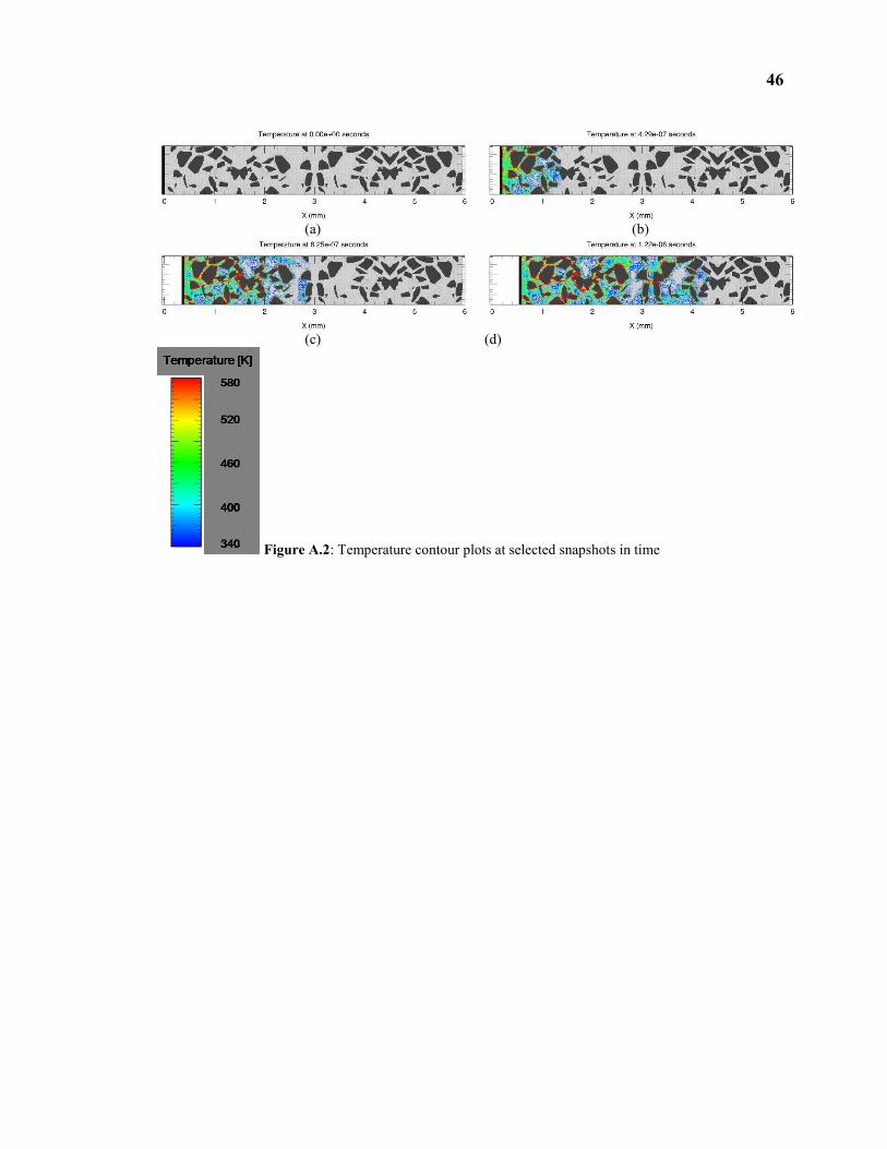
46

(a)

(b)

(c)

(d)

Figure A.2: Temperature contour plots at selected snapshots in time

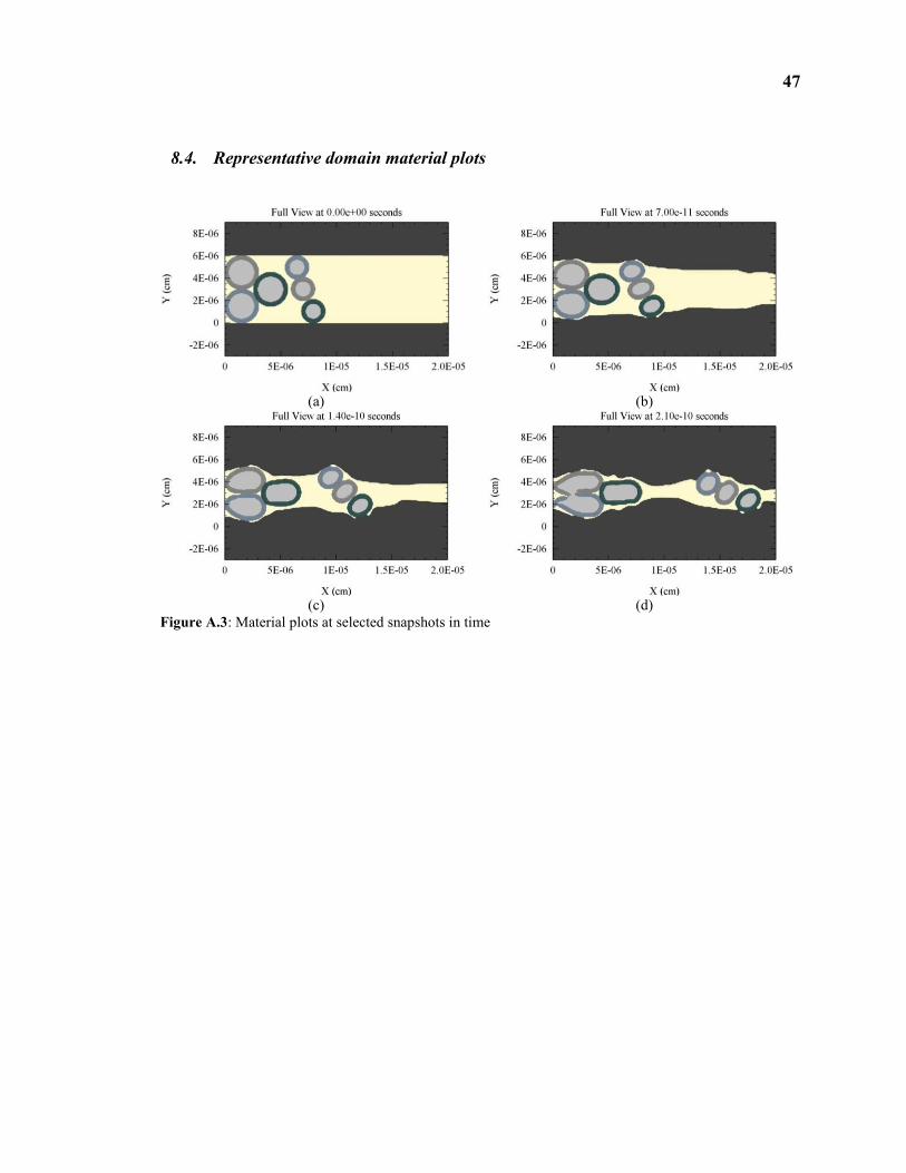
47

8.4. Representative domain material plots

(a)

(b)

(c)

(d)

Figure A.3: Material plots at selected snapshots in time

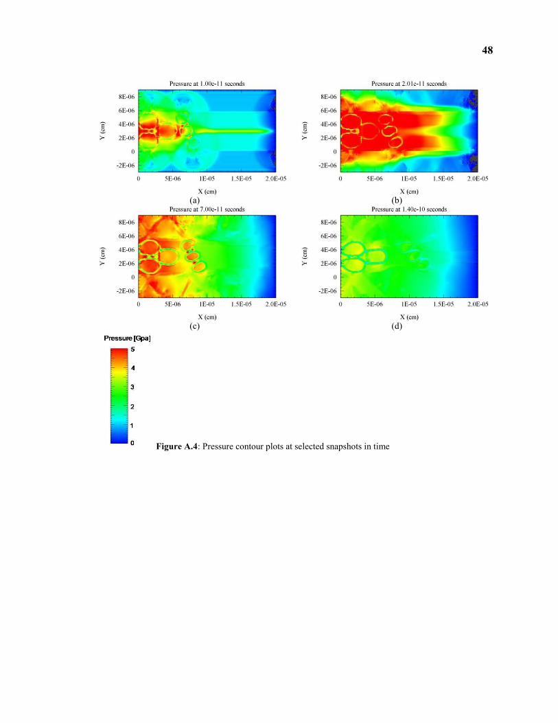
48

(a)

(b)

(c)

(d)

Figure A.4: Pressure contour plots at selected snapshots in time

49

(a)

(b)

(c)

(d)

Figure A.5: Temperature contours at selected snapshots in time