Methods and aspects of active-RC filter synthesis

van Bokhoven, W.M.G.

Published: 01/01/1970

Document VersionPublisher’s PDF, also known as Version of Record (includes final page, issue and volume numbers)

Please check the document version of this publication:

• A submitted manuscript is the author's version of the article upon submission and before peer-review. There can be important differencesbetween the submitted version and the official published version of record. People interested in the research are advised to contact theauthor for the final version of the publication, or visit the DOI to the publisher's website.• The final author version and the galley proof are versions of the publication after peer review.• The final published version features the final layout of the paper including the volume, issue and page numbers.

Link to publication

Citation for published version (APA):Bokhoven, van, W. M. G. (1970). Methods and aspects of active-RC filter synthesis. (EUT report. E, Fac. ofElectrical Engineering; Vol. 71-E-27). Eindhoven: Technische Universiteit Eindhoven.

General rightsCopyright and moral rights for the publications made accessible in the public portal are retained by the authors and/or other copyright ownersand it is a condition of accessing publications that users recognise and abide by the legal requirements associated with these rights.

• Users may download and print one copy of any publication from the public portal for the purpose of private study or research. • You may not further distribute the material or use it for any profit-making activity or commercial gain • You may freely distribute the URL identifying the publication in the public portal ?

Take down policyIf you believe that this document breaches copyright please contact us providing details, and we will remove access to the work immediatelyand investigate your claim.

Download date: 05. Jun. 2018

METHODS AND ASPECTS

OF ACTIVE -RC FILTER SYNTHESIS

by

W.M.G. vanBokhoven

i

Eindhoven University of Technology

Eindhoven The Netherlands;

Department of Electrical Engineering.

METHODS AND ASPECTS OF ACTIVE - RC FILTER SYNTHESIS

by

W.M.G. van Bokhoven.

T.H.-report 71-E-27

ISBN 90 6144 027 0

10 December 1970.

Submitted in partial fulfillment of the requirements for the

degree of Ir. (M.Sc.) at the Eindhoven University of Technology,

Department of Electrical Engineering.

INTRODUCTION

Ch. 1.1

1.2

1.2.1

1 .2.2

1 .2.3

1. 3.1

1 .3.2

Ch. 2.1

2.2.1

2.2.2

2.2.3

Ch. 3.1

3.2.1 3.2.2 3.3

Ch. 4 4.1 4.1 .1

4.2 4.3 4.3.1

11

Approximation. General low-pass filter approximation. Butterworth approximation. Chebychev approximation. Elliptic approximation. General properties of the elliptic trans­ferfunction modulus.

page 1

3 3 5 6

7

8

Algebraic derivation of second and fourth degree elliptic transferfunction modulus. 12

Network sensitivity. Sensitivity functions for second order low-pass LCR-filters. Sensitivity calculation for an active low-pass filter. Sensitivities for the Fj§lbrant filter.

Active filters obtained by substitution

20

21

24 25

methods. 27

Gyrator-capacitor substitution. 27

Gyrator circuits. 28 Active synthesis using frequency dependent

negative resistors. 33

Active filters on synthesis basis. 38 Negative Impedance Convertor synthesis. 38 Sensitivity considerations for the Linvill-synthesis. 41 Synthesis method of Yaganisawa. 43 SyntheSis with the gyrator as a two-port. 45 Sensitivities for the RC gyrator two-port synthesis. 48

iii

4.4 Synthesis with PICs by the Antoniou

method.

4.4.1

~. 5

5.1

5.2

Special cases for the Antoniou method.

Cascade synthesis with second order sec­

tions.

Second and third order low-pass Fj~lbrant

filters.

Active realizations of second order Notch

filters with a modified Twin-T network.

49

51

54

54

56

5.3 Active filters employing negative feedback. 57

5.4 Second order filters with PICs. 60

Appendix. 61

References. 68

INTRODUCTION.

In many fields of electrical engineering filters are Co

used perform or equalise amplitude, fase as well as delay characteristics. The circuits becoming more and more com­plex with the refined application of electronics nowadays, need for microminiaturisation in order to limit the physi­cal size to a reasonable one.

In the last ten years great progress was made in mi­niaturising resistors and capacitors as well as active elements however inductances still kept their same size because a certain volume is needed to store the magnetic energie connected with the value of the self inductance and the current flowing through it. Only magnetic materi­als with a higher permeability would improve the quotient inductance-volume and with the state of the art of ferro­magnetic materials at this time no revolutionary progress

has to be expected. On the other hand the tendency is growing in reali­

zing complete circuits in monolitical form on one chip of semiconductormaterial, filters included, to get better stability and reliability at the same time.

Since classical filter synthesis leads to the use of inductances together with capacitors and resistors, it's impossible to design integrated filters with this method, unless the inductances are simulated in one or other way.

This simulation can be done by means of gyrators wich method has the advantage that one can use known syn­thesis methods and merely replaces the inductors by gyra­tors terminated with capacitors. From synthesis point of vieuw there will be no trouble, however a lot of active components are needed so that the circuit in general

1

2

won't be an economical one and the simulation of floating inductors demands for an even higher complexity.

As a second possibility the gyrator, being passive

however mostly build up with active elements, can be used

as element in a new synthesis method based on R-C net­works coupled with the gyrator considered as a two-port network, trying to make full use of its property's and thus in a certain way minimising the number of implicit

active elements. Also negative impedance convertors and vario~s other active elements can be used to realise fil­ter networks on a synthesis basis each having its own ad­vantages, limitations and disadvantages.

The third method consists in fact in splitting up the filter transferfunction in first and second order

parts, each of wich can be realized by a suitable active

circuit together with R-C elements.

Because of the great number of active second order filter realisations a wide variety of circuits is possi­ble and one has to use extra design criteria, not always being electrtcal ones, to make the best choice.

The intention of this paper is to describe and com­pare some lumped R-C active filter realisations and syn­thesis methods of the above three groups on a basis of sensitivity and stability, wich ap~~ to be usefull criteria for practical utilisation of the designed filters.

. ~ As apparent from the forego~ng for shomness sake no attempt has been made to investigate the wide class of digital and switched filters, although these methods be­

come more and more promising in the near future.

1. Approximation.

1.1. Electric filters are used to realize prescribed input­output relations for the signal passing through. These relations may be given in terms of amplitude or phase response of the given signal or otherwise be specified. Generally these specifications are given as a tolerance field in amplitude and phase frequency characteristics while mostly only one of them will be prescribed and the other one is concerned to be of no importance. The filter to be designed has to meet these specifica­tions i.e. must lead to a response full filling the to­lerance conditions being set. Thus the filter design starts with the determination of the transferfunction from the prescribed limitations where after this trans­ferfunction must be synthesized. In order to present a more closed description of the synthesismethods some of these approximations will be treated in the next chapters, mainly following ref. (1) in notation and deri va tion.

1.2. The general low-pass filter approximation.

An important class of filters is formed by the so called low-pass filters, wich approximate the modulus of a transferfunction in such a way that signals with their frequency ranging from zero to the frequency fo will be passed without much attenuation while signals with fre­

quency exceeding fa will be strongly attenuated. The to­lerance field for this type of filters has the general form of fig.1. Here in the frequency axis is devided in three main parts, ObVio~sly characterized as:

part I - passband part II - transition band

,.. part III - attenuation band or stopband

3

I HI! nl\ ~.L...L.~~--'--''-L.., i

fig.1 •

.z 1--

Constructing a transferfunction from a given tolerance

field is accomplished by derivation of the modulus as

a pure mathematical approximation of this tolerance field with an even function of the radiant frequency. Here after the transferfunction itself is obtained

from the constructed modulus on a basis of network theo­

retical prescriptions.

The above mentioned approximation can proceed as fol­lows.

Let the modulus to be approximated be the modulus of a voltage transferfunction H(p) defined by

~ ~~t = H(p) and p = jA , where in V~±R and V d~t

are the amplitudes of the sinusoidal steady-state exi­

tation and response.

The squared modulus of the lowpass filter can be written

in the general normalised form as l

/ HtP2)/ == 1

Here in ffj(.n.) is an even or odd function in.Il called the characteristic function and H is a constant. Defining the transfer loss ~ as

0( = - 20 log Ii ,,''':'''J.1 dB /1I(J:.t1)/

4

this leads to

l J " 0(. = 10 log [1 + H ~ (.o.~ dB (2 )

In this notation the modulus indeed is characterized by the choice of the characteristic function.

1.2.1 Butterworth approximation.

Taking §(.n.) = ..n."

leads to the Butterworth or maximally flat approximation based on the property that in the point.Jl =0 the first 2n-1 derivates of the denominator of (1) become zero, resul ting in a flat pass of the curve near 11 =0. Further­more the denominator increases monotonically with it lea­ding to a monotonic fall-off for the modulus i~self. For the Butterworth type from (2) and (3) this results in an assymptotio increase in transfer loss with 6n dB per octave for R.n."'» 1 • In fig. 2 'some of these curves are drawn normalized for equal.Jl , being the frequency • where oC is 3 dB down. Dt----------==:~~

-I() o.r 4 I,., fig. 2. Normalized Butterworth low-pass transfer-loss.

For this type of approximation there will be no difficulty in selecting n and H that way, that the resulting loss characteristic is lying in the given tolerance field.

5

For a rapid falloff in the stopband however a large n is needed leading to an excessive number of filter ele­ments as compared with the Chebychev approximation given in the following chapter.

1.2.2 Chebychev approximation.

By taking 111 (..0.) = Tn (n)

with Tn (.0.) = cos 1: n arccos...1l.] forll.~ I (see fig.3)

a 'chebychev approximation is obtained. Tn(.fl-) can also be written as

t;] '" I 0.-.'" Tn (.fl.) '= :!: ~ (-I) ( .... -""-1). (Ul) (s~e ,.~, [:lJ)

2 L- ?nl{"'-l"')' ?rtc.o • •

The passband ranging from.il = 0 to.1l = 1 shows n /2 equal amplitude ripples between a minimum and a maximum value

determined by the constant H. In the transition and stopband (11 > 7 ) A'Tn (.Il.),f increases monotonic with J1 again producing an assymptotic increase in transferloss of 6n dB per octave. In comparision with the Butterworth approximation the value of n can be taken smaller for the same tolerance field leading to fewer elements in the final realisation. Some chebychev characteristics are given in fig. 4. Because the extrema of Tn(JL) in the passband all have modulus 1 the ripple amplitude is determined by

a'r= 10 log [1 +H2] dB (f.,11 ...

of

f

fig.3 Chebychev function Tn(11) fig.4 Chebychev low-pass transfer-loss

6

1.2.3 Elliptic approximation.

As stated in 1.2.2 introducing a ripple in the pass-band leads to fewer elements in the final realization. As a consequence this suggests an approximation having also ripples in the stop-band, probably will reduce further the number of elements as compared with the previous chebychev type. Specially if the number of stopband ripples is taken to be equal to the number of passband ripples a so called elliptic approximation is obtained if gj"{A) satisfies certain relations expressable in Jacobi ellipticfunc­tions. This type of approximation leads to points of infinite attenuation in the stopband, together with a fast fall­off in the transitionband. Because the relative few number of elements needed to approximate a certain attenuation this filtertype is an interesting one for application in active filter design where, as we'll see later on, the sensitivity plays an important role and the more complex a network is, the more difficult it will be to realise .. the filter with the required accuracy and stability. Unfortunately however the calculation of the transfer­function for a given tolerance field is much more diffi­cult for this filtertype as compared with the previous ones but the gain in simplicity for the final network

makes the effort worthwhile. On the other hand it ap­pears to be easy to calculate the transferfunction in an algebraic way if the degree of the filter is small (up to 4). Therefortin the following the algebraic method is ex­

'" .,., ",lIthe/"1( plained first and latep en the formulas will be given for the calculation of the higher order filters.

7

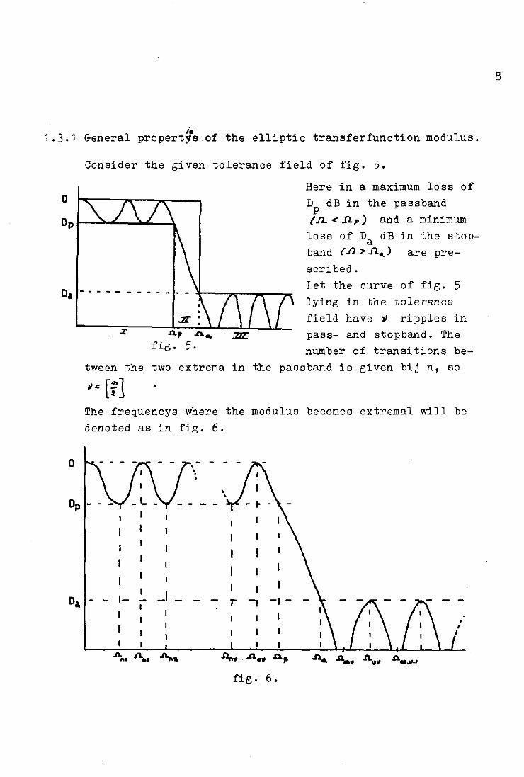
ic 1.3.1 General propertys.of the elliptic transferfunction modulus.

o

Consider the given tolerance field of fig. 5.

Here in a maximum loss of Dp dB in the passband (n_ < .n1') and a minimum loss of Da dB in the stop­band (.n > 11 ... ) are pre­

scribed.

Da--------- Let the curve of fig. 5 lying in the tolerance field have V ripples in pass- and stopband. The number of transitions be-

r 4, .n. .. fig. 5.

tween the two extrema in the passband is given bij n, so

•

The frequencys where the modulus becomes extremal will be denoted as in fig. 6.

Da - - 1--I __ _

fig. 6.

8

L

According to (2) 0( = 10 log [1+ H~"r.Alj

From this follows that the pOints of zero loss correspond to points wi th ~(.n.) = 0 as well as the points of infi­ni te loss correspond to ~(n) = 00. On the other hand at the points.n. wi th s=1, 2, ... II, 0(. has a local minimum, ns . and therefor ~(llns) is local maximum. In the same way one concludes that m (n"s> is a local minimum. Denoting the maximum absolute value of ~(JV in the passband by L and its minimum absolute value in the stopband by K, the charac­teristic function can be drawn as indicated in fig. 7.

~(n)

t IVI

- - ~ -:-I : , - -I

. A I I

From the foregoing fol­lows that the function Iff [...Il.) has to be an

even or odd rational function of...n... because

becomes infi-r¥ ., 11", II .n. ..

O+-::-'-Ij'------'----T'M~-IL__f!!!II!E~___,~--=-: .1\,/::, ni te in the points.ll • "'$

In order to determine I • .J'II.", _L _ _ _ I

/jfn) we could chose

-I(

.n.w : 1 I I

------ ~ -:-A -:-fig. 7.

a rational function of sufficient degree with undetermined coefficients in the numerator and de-

nominator polynomials and then derive equations for these co­efficients from forcing all extrema to have amplitude L in the passband and amplitude K in the stopband.

There exists however a more easy way to obtain the same re­sult by the following reasoning: If we are able to relate the behaviour of ~(J.L) in the stop­band to its passband behaviour in such a way that the right passband behaviour automatically implies a right stopband behaviour, we would only have to consider the passband of ~(J.L) ,thereby halving the approximation problem.

9

Let therefoI?the frequency be normalized such that

..1l. p Jl .. =: t

and ~(n.) = /

(3)

(4)

Equation (4) relates the value of !/!{.n.) in the band ..12 ~ 1

to its value for J'l':::.d ~ t in a reciprocal way. This im­plies that an equiripple behaviour for ..(l. <! ~ also gives equiripple behaviour for.n.~ 1 Furthermore for frequencys .1l. os lying in the passband

o ~.1l. ~ ..fl p < 1 we have

~ (..flos) =: 0 or" 1,1, ...• &I.

as a consequence of (4) this results in I

!§(Ji;;)'" 00

I

and thus (4) implies

Also a maximum value of ~(..fl)in the passband will lead to a minimum value of ~(.n.) in the stopband related by

7Ir{ ~L= I =_-1- I JIt! ..n..". ) = ",; '" u ~ ,:J'l."s) " (6 )

and .1l"s -/ (7 )

As a consequence of (3) also .11 .. = .Ap

I (8)

relating the bandedge frequencys in a reciprocal way too. From (6) follows k:- -i: expressing the stopband ripple of

;r.n.) in its passband one.

The above points out that relation (4) indeed connects the

10

stopband in a one to one correspondence with the passband satisfying all the nescessary conditions.

Taking p(n). 7l' /.. (.Il) .. ,.(.fl.)

1[ Ida) = 7l ,itt) i ,.-{fl.) I Ii f.;f.)

together with (4) leads to

This relation can be satisfied if Idll)" Pf:if:.J leading to

Because

~(.fJ.) ::

~(.b..) ble choice for

must pr..n.)

become zero for 11. rJl"s , a reasona­will be

• n • 7l: ..n.. -"'~ ... ' . , A' 4 .n:' - .J~tI.

resulting in

(9 )

is ,n.... also satisfies equation (4) we can transform (9)

into

• • §l.n..J " 7l: .Jl. - .11 •• i -Ile..n.;. _ I for even

for odd

.ilFf.n...) l §j'fAJ J

(10)

From (2) and (6) the value of 1 and H can be calculated giving

1> .. =

wich leads to l' d.' D" ) ( A' D.. ) I H = (10 _ I /0 - I

"" + 0., ZIo. L ¥= ('10 - 1)/(10 - " )

( 11)

11

1.3.2 Algebraic derivation of second and fourth degree elliptic transferfunction modulus. For second degree IJ{A.) equation (10) leads to

$(.11.) c ..A~ - .fl."," JL":f1I1'~ _ / ( 12 )

This function is shown in fig. 8.

It n,.,

-Jl.,&

I --. JI.,

..n. -

From (12) we get Zt'D) = ft.,'w L.

There..--for ..fl., =- fi

It,," ..n."", = j/n-

Then AI' follows from !F fA,. )1-J1., ~ = -L

Jll> = r,g; } Ji7&

..n.& • , -fip

giving

From (14) the selectivityfactor "" defined by becomes

(13)

(14 )

(15)

12

For quick reference k can be determined from fig. 9

for given Dp and Da.

Da

50

40

30

20

10

Dp 1235 dB 11 J I

0.1 0.2 0.3 0.4 0.5 0.6 0.7 0.8 o~ fig. 9.

K

The above formulas lead to the following designproce­dure 1. Determine from fig.9 if the given Dp and Da will

lead to a satisfactionary selectivity factor k.

Otherwise a higher order filter must be designed. 2. Calculate Land H from eq.(11).

3. ~t-a) follows as

TCil):: ...n. ~ - Jl.o1 .{

A~o/- / wi th AO/' rF

/1-I(j.4)/.t is given by (1).

4. The various characteristic frequencys follow from ( 1 3) and (14).

5. Here or afterwards use a frequency transformation to obtain the desired values for the frequencys of point 4.

For a fourth degree approximation two terms in (10) are needed.

13

In order to simplify the calculation ..a .. ", is set equal to

zero wich appears to be equivalent to a certain frequen­

cytransformation operated on the normal fourth degree

approximation leading to the so called "bar-type" fi 1 ters

in ref.[t1. At the same time this results in a zero in

/ H{f.AJj as..n. approachas infinety.

So /Etn.) becomes

wi th its graph shown in fig. 10.

~(./J)

t

'I>~ - - - ~ __ "'"

-\,/ ,

I ,~ ______ ~ __ ~~~n~~~~.~'~~~~' ______ __

.A",

-~ - - - - - - - - --

• I , I

I

I r-

Fig. 10.

.JL ...

To derive 12111 from (16) one proceed as follows •

(16 )

.12", is determined by the quadratic equation 4J1Ay,,) =- i.. Because :E!.il) is tangential to the line (6 = i. the

previous q.ladratic equation has two coincident roots

and therefor zero discriminant.

15 (.fl.,,,,)" L wi th .12/1, •• k lead s to

"~-.Jlo,~r,..")~ .... L = 0

Forcing the discriminant equal to zero gives

./ZD, ¥ (I"~) ~ - "i • 0 resul ting in

and

A tU = li~:;]~ ~

.12 .. , ~ %Z .. " j (17 )

SO

40

30

20

10

0

The solution of the quadratic equation becomes :t: = ...fJ.",~" JIZ

Therefore

fiAI = ,;yz-r .A.VI = / / tYL' }

and

At last ftp follows from

;t.Jlp)= -L giving

J21' • = -A» ht.. = -4 ~

(18 )

(19 )

In fig.11 the selectivity factor k is given in depen­

dence from Dp and Da.

Da Dp 1 235 H ~ \.

0.1 0] 0.3 0.4 0.5 0.6 0.7 0.8 0.9 1.0 fig. 11 •

Design procedure

1. Determine from fig.11 if the given Dp to satisfactionary selectivityfactor higher order filter must be designed.

2. Calculate L and H from eq. (11). 3. ;1.J1) follows as

1§"( J1.) ., .A.. J). a_ ..Il.o, .. .L2,I.Il., f _ / wi th

I /{(jAJj~ is gi ven by (1)

K

and Da will lead k. Otherwise a

15

16

o. 4. The vare1us characteristic frequencys follow from (17),

( 1 8) and ( 19 ) • 5. Here or afterwards use a frequency transformation to

obtain the desired values for the frequencys of point 4.

1.3.3 Derivation of the transferfunction from a given mOdulus.

The modulus of a transferfunction is determined by

/ IltJ"J1.J/ ~= /lIp). H~,PJ I P-dA.

~

This equation immediately shows that /#(/4)/ is an even

(20)

.t function of.n.. , thus only approximations for /1I(,fJaJ/ wi th even functions can be tolerated. Defining 1/(.4) = :r;? 'F)V/II(j.nJ/:Ve have from (20)

1./(.1): II(I').H/-p): (b(p) ,) (21 )

Herein~~)is a real rational and even function of p and can be obtained from /HIj.n)/·by substituting ..Q."c -pI.

As /1I(i.n)/~ ~ 0 thi s implies that (J) C f»">'- 0 for imaginary p.

Therefor the zeroes and poles of ~(p) on the imaginary axis must be of even multiplicity otherwise ~(p) would change sign in these points. The stability of H~) however requires the imaginary poles of (Jl(/,) to have mul tiplici ty 2. BecauseAKI') is a real rational function of p , its complex poles and zeros arrise in complex conjugate pairs. On ac­count of (21) the complex poles and zeros of ~I')will then show quadrantal symetry. Real-axis poles and zeros of ~(p) are each other mirror­images w.r.t. the imaginary axis. As in the resulting H(,,) the poles must ly in the left half plane with single poles on the imaginary-axis to insure stability, we can construct AI~) from the above

(ifp) by assigning a pole-zero pattern to H~) consisting

of all the poles and zeros of Q(p) in the left half-plane and half of its poles and zeros on the imaginary-axis. Then automatically H(p).H(-p) has the same poles and zeros as Q(p) because H(-p) has the mirror-image pole-zero pat­tern of H(p). The in this way constructed H(p) is called "minimum-phase" transferfunction.

1.3.4 Numerical example of a fourth-degree approximation.

Suppose one has to design a low-pass filter for use in telephone-links having the following specifications:

Passband edge-frequency 3400 cis Stopband edge-frequency 4500 cis Passband ripple 3 dB Stopband ripple 30 dB

The design starts by calculating the prescribed selecti­vity factor k giving

-,,, -!!:.e ,. .tlr. '''''0 ~ .,. '1~ A... A'~. 41$'1'0

Following the five steps of chapter 1.3.2 results in: sub.l. From fig.11 it can be seen that the given losses

will lead to a selectivity-factor k=0.81 wich is certainly better than the required k=0.75. (One may alter Dp or Da to get closer to k=0.75 for example by taking Dp= 2 dB and Da= 30 dB giving k=0.78).

sub.£. sub . .,l.

From (11) follows L=0.1776 and H=5.6153. (17) gives Jl", =0.846063 and.n. =1.181945 ..., This leads to

18 (A) = Jl ~ .12'- ... "fllf" ~ Jl .... tPfI({I'- I

Then (1) gives • I (o.>,.zA.~-I)

/#(IN/ ~ I'" N'T{A) " .I/o ~JA.d_ 4f~. "'~.Jl <I". /~.Ifi'.Jl" - /. ¥.1A~ "./

17

sub.±.. From (18) and (19) fo 110IVS

fl.,. =0.90 .12 ... =1 .11

..n.", =0.65 .Alii =1.54

sub.2.. The passband edge-frequency of sub.4 being.J2,. =0.90 has to be transformed to the desired one given by

t.J" = .t1l·3400= 21363 rad/sec. Thereforea frequency transformation must be made by su bsti tu ting

0.90 0 0 421 l'n /HI;""I/~ .n.. = 21 363 w = . 000 (,J ~

Its however more easy to make this transformation after the whole transferfunction is realised by changing the final elementvalues with a proper factor. In this way the calculation proceeds with coefficients and elements being of comparable value thereby reducing the chance on making errors in

the computations.

For calculating H(p) we find from (21) (0. 72p2+1 )2

Q(p)= 8 6 4 2 31.53p +45.14p +16.67p +1.43p +1

The poles of Q(p) follow as the zeros of the above deno­minator giving

P1,2,3,4 = + (0.06092 + j 0.86747) P5,6,7,8 = + (0.36631 + j 0.31825)

The zeros of Q(p) are found as

P1,2 = + j 1.1819 P3,4 = + j 1.1819

From the above we find the poles of H(p) as

P1,2 = -0.06092 + j 0.86747 P3,4 = -0.36631 + j 0.31825

18

19

and its zeros as

P1,2 = ±. j 1.1819.

Then H(p) becomes

H ( p) = O. 17 807 (p2+0.12184P+O.75622) (p2+0.73262p+0.23547)

dB o The resulting apprximation is given in fig. 12.

Or-----------------------__

10

20

30

~ ____________________ ~ ________ ~ ________ +-____ .-__ .L~ __ ~~ ... KHz

·1 ·s 1 2 3 4 5 S 7 '0

2.1 Network sensitivity.

Any transferfunction of a network is as function of the network elements sensitive to element variations. The network structure capable to realize a certain transfer­function having the least sensitivity compared with other structures is thus the favourable one for use in the syn­thesis, because unavoidable tolerances in the element va­lues will then have the smallest influence on the reali­sed transferfunction. It is then reasonable to use the sensitivity as a basic criterium in the network design, especially in active filter applications wich can be very sensitive, in order to assure that the transferfunction can be realised with sufficient accuracy. For the comparisfD~ of the various possible structures its thereforenessecary to have a

measure for the sensitivity. Depending on the type of transferfunction and its application, various definiti­ons are used, the most current of them given below.

W(p,r) W(p r) S defined as S ' = r r 1. Parameter sensitivity r QW(p,r)

W(p,r) ~ r Here in W(p,r) can be a transferfunction, transferloss, quality factor etc., with parameter r.

2. Pole- or zero-sensitivity sq. If q= fFCI')+3"./l{l') is a r

pole or zero of some transferfunction,S i is defined as ... ,. ~r .,. "A-

S,. = -; ;;~/E j7 "

The following derivation may simplify the application of the loss-sensitivity. As rt. = -10 log /I-I(;"t.>y~ we have

.r". ~ a r-I0.,J..,/I,'QIoJ>!' J ,.,. .....:;1 __ I' 11(, tJ ,. • -J;;; jj( / N(jI.)/'

·,N"....-· J - Ii. • ¥ . .It' H91"H~,oJ = ~ s . . - - S ~.-I"II' r " I' / .. ,41

(22)

From the definition we can derive

20

21

s W(p).V(p) = s W(p) + s V{p) r r r

\'Ii th (22) this results in III ~[r N~' f r HE-III]! . .r r '" - t( J,. J,. jI_JtJ

leading to

.f " . th ,. .... tJi,. ~ Wl. J - we - .,,, finally have Approximating

A til' • - tt'. ~" He [s ':<; ... '/ ~,. (23 )

A ~,. • -

2.2.1 Sensitivity functions for second-order low-pass LoR-filters.

In active synthesis a frequently used method consists in deviding a transfer function in second order parts wich parts are then realized with suitable active circuits and

cascaded by inserting isolation amplifiers if nessecary. The overall sensitivity of the resulting network then de­

pends on the partial sensitivity of these second order

sections. It is therefore convenient to compare the active second order filter sensitivities with those of a passive one realising the same transferfunction, because we have

a lot of practical experience with this filtertype and need a reference anyway. Let the passive equivalent be given as in fig. 13.

l

+ E c

1-.,. I~.

A straight-forward calculation sholVs the voltage trans­ferfunction to be

V2 H(p)= E = (24 )

From (2;')

P1 2 ,

the

= -

following poles results: 1 . 1 1 2 . f i

2RC ± J 1C - (2RC) J.f

':li th 1 ~ 1

(J" = -2RC '-'0 = 1C and Q = R rcA. "7 this becomes

= (J"::t i4Jof 1- (~)~ wi th Q ;> ~

This leads to the following pole-sensitivities: S'" ''/ 1-1' ... - .(..1 .1..)

c ~ -I-J·.l 1_ ,/.,,,& ~ -I -J '" - 'f •

,. S ~ •

./

~.) .. ~ -Jft' -J 1- '1".·

_/ ~. of ~ -/ ~ i· ff,~. ; +','-1

r " • It •

(25)

More over the Q-factor sensitivity as well as the resonant­frequency sensitivity follow as

s ct " ~ s· s ""=

.... -1t .-~ .,,'" S = (26 ) • l C

s· .. = 1 S OJ.

It "0

Calculating the loss sensitivity one finds II{jIolJ c ,)1-1(,)/ &oJ.,t. c

S • -. 7C p.Jt.J =:

,-",'L.e ~.;i""~ '" H{pJ

Normalising the frequency (J to the resonant frequency "'0 by substituting ..Il.'~ we find:

Then

and

S H():nJ. A" C I-A" ., j :E::.

(23)

A"'c=

<l1

results in At: --12. f (I-A.')

-~[s ~)I -= ft-.nt) .... ~ c

-Jl. ~(I_.ft') .,. .J1'l4;t.

V-A")' .. ..12&/".

AC. .11"'-" .. 7'.

22

The maximum values of these loss-variations for large Q-factor become

.6 Ofc ". .. , ~ :t ~. ~ lIIe/,,," ~

..0 ~ ..... ... .t ~. ",L :t 7: Nc/,_ ..

.Q ~ ....... <\: -,.. • ...... N~I"" ;i'

The above variations are shown together with the norma­lised transferlo$s ~ in fig .. 14 for Q = 5 and element variation 1%.

Ii. l'

-12 d.B

-8

-4

0

4

8

12

..00(

t

r +-

.1

,2

,3

16L---~--~-T~~~~ __ ~~~-: ______ ~ __ _ .1 .2 .4 .8 1 2 3 4 .1l. ....

23

24

2.2.2 Sensitivity calculation for an active second-order low-pass filter

+

Consider the active fi 1 ter in fig. 15 where in the opera-tional amplifiers are supposed to be ideal.

11 I

~~~~--r-------~.~ This results in the same R1 R Dotential for the points ,

+

v

c

A,B and C. The potential-devider R R . V Vo V

3- 3 g~ves c~~ 2 V Therefore VB = £ and

v.. - v. ~C, I,

' .. = ~j :I ~." 'I'C, .,

This current i2 flows into the resistor R2 re­

sulting in a voltage drop over R2 given by /' (", .t& • /I ..

Because VA = VB the same parallel combination R-C it follows as

voltage-drop must fall over the .. ~ence the current flowing through

1+pRC i1 = R • V.

On the other hand VA is given by

VA = E - R1 i1 = ~ Suost::.tuLing i1 in this formula and solving for ~ gives

V 2 E = p2R1R2C1C+P R1~2C1 + 1 (27 )

If we take R1R2C1= L we find formula (27) except for a constant factor to be exactly equal to formula (24) wich resulted from the passive filter in fig. 13. Therefore we can conclude immediately that the sensitivi­ties for the active filter given here are the same as those of the passive one dealt with in the previous chapter if

we make the following correspondence:

is always stable for every positive value of the elements.

The root-locus is therefore confined to the left half-plane.

Furthermore (27) and (28) indicate that this active filter

only differs from the passive one in the sensitivity w.r.t.

the equivalent L being three-fold instead of a simple one.

The influence due to the non-ideality of the amplifiers

such as finite gain etc., is kept out of considerations be-ol

cause this influence is small if the amplifier ban~ith

is taken to be large enough i.e. exceeding the frequencies

of interest for the filter.

A sure advantage over the nassive filter however is that

25

any impedance !:lay be connected to the outnut terminals

without the transferfunction being changed. For this reason

this filtertype is very well anplicable in cascade-synthesis.

2.2.3 Sensitivities for the Fjtllbrant-filter.

The Fj1ilbrant-filter [3] or Sallen and Key filter in

fig. 16 is another active filter capable to realize se­

cond-order transferfunctions however with much larger sen­

sitivities than the fore~going one, in such a way that this

filter can only be used when low to moderate Q-factors are

dealt with.

From fig. 16 we easily calculate

H(p)

+

o

+

v

o

fig. 16.

A close look on the above

transfer function shows that

in the case that A becomes

large the coefficient of P

may become negative, r~sul­

ting in ri~ht half-plune

poles and thus H(p) becomes

unstable as can be seen from

the root-locus of fig. 17

with arrowdirection corres­

ponding to increasing A.

From H(n) the ~

sensitivities are computed as

S" ::

4 0(" ".( Q .... 411 If N~l'r,. } (29 )

If the values of (29) are compared with those of the

passive filter we find them to be much greater. Especially

s~ becomes large for moderate Q-factor because in this

case I[R1 Cl ::: Q leading to SAQ

l::S AQ2. V j'2 C2

On the basis of the fore­

going comparision we have

shown that active filters

realising the same trans-

R .. .,. ferfunction can have dif--*~~~~~--~4--+--

A-co ferent sensi tivi ties, nos-

sibly being equal to or

better than the passive

26

one s as well as being f !i~",,.,,IIJ worse.fenly low sensiti-

vities vdll guarantee good

fig. 17. agreement between the wan-

ted and really obtained

transferfunctions. Hence one should prefer the slight more

complicated network of fig. 1$ above the Fjalbrant-filter

when moderate or high Q-factors are needed.

However large pole-sensitivity does not always imply large

filterloss sensitivity as can be seen from equations (25). If we take Q<= -$-, we find S ~'" -l-j... indicating that the pole-sensitivity becomes very large due to the large rela­tive change in the imaginary part. The filterloss for small Q-factors is however mainly determined by the real part of

the poles and is therefore much less sensitive to element

variations as one would expect from the large value of S ~. On the other hand small pole-sensitivity is not always coupled with small loss-sensitivity but in most cases the

lower the sensitivities are, the better the filter will be as to the influence of parameter changes.

If the filter poles are determined by a difference of two polynomials each with positive coefficients, the resulting polynomial shows large coefficient sensitivity for the

smallest coefficients because these coefficients are ob­tained by substracting almost equal large numbers from each other. Therefore one must avoid synthesis methods

leeding to coefficients wich are determined by a difference of products of the element values. However if every polynomial coefficient consists only of the sum of products of the element values, the filter still

can be very sensitive to element variations. For example the polynomial p3+p2+1 ,Olp+l is a Hurwitz polynomial while p3+p2+0 ,99p+l has zeros in the right half plane and thus leads to instability if this polynomial would determine

the poles of a transferfunction. Hence a slight change of

one coefficient due to a change in one of its composing

products may result in instability even if this coefficient is build up with positive sums of these products. On account of the foregoing one may conclude that the sensi­

tivity plays an important role in the design of stable and insensitive networks but large or small sensitivities on their own are not absulute criteria for the behaviour of the designed filter.

3.1 Active filters obtained by substitution methods.

The synthesis of active filters will solely involve known

nethods if they can be deriVed from the r>assive filters

in some direct way. In this case one uses nassive synthe­

sis methods to construct active filters by changing the

nassive filter so as to eliminate the ar>pearing inductan­

ces.

The mainly used methods hereto are replacement of the in­

ductors by gyrators and capacitors as explained in the

following sec tion and imnedance transformation as wi 11 be

given in section 3.3.

3.2.1 Gyrator-capacitor substitution.

Consider the circuit of fig. 18 where in the gyrator is

defined by the following non-reciprocal two-port admit­

tance-matrix

(30 )

Connecting an admittance Y. to the post 2_2 f gives an

input admittance

Y-.. = '1/,," 'f/, yu = ~:.. ,. ''''YJ .r. 2

Especially for YL= PC we get Yin= gc = p~2c' being the

admittance of an inductor with inductance L = R2 C Henry.

Therefore this configuration can be used to replace in­

ductors in a passive LCR filter. As an examnle a third­

order Butterworth low-nass filter is then realised as

depicted in fig. 19.

27

2

1 2

1 1 1

c

l'O--L ___ .J"7' 2' ~ nrlr--r-......, G .1

1 ,....-02 1 1 1

2

1'0--..1 .... --02'

fig. 18. fig. 19.

On sensitivity point of vieuw this network only differs

from the original LCR-filter in the sensitivity due to elements in the capacitor-gyrator circuit.

O"clt ... ,." _ As was indicated by Hi i dan L'IJ this leads to low-sensi-tivity of the resulting network as compared with other

active circuits with the general tendency as to shift the poles further away from the imaginary axis. Hence the net­work is always stable.

3.2.2 Gyrator circuits.

For the gyrator to have good quality, i.e. approaching

(30) as much as possible, one uses electronic circuits to construct it. The main point of interest lies in the

diagonal elements of (30) wich must become as close to zero as possible however remain positive. To demonstrate this point consider the non-ideal gyrator admittance-matrix r G, G.]

[~1 = r(;' t:~

Connecting a capacitance pC2 between the output terminals gives an input admittance

G G Yin = G1 + 2 3

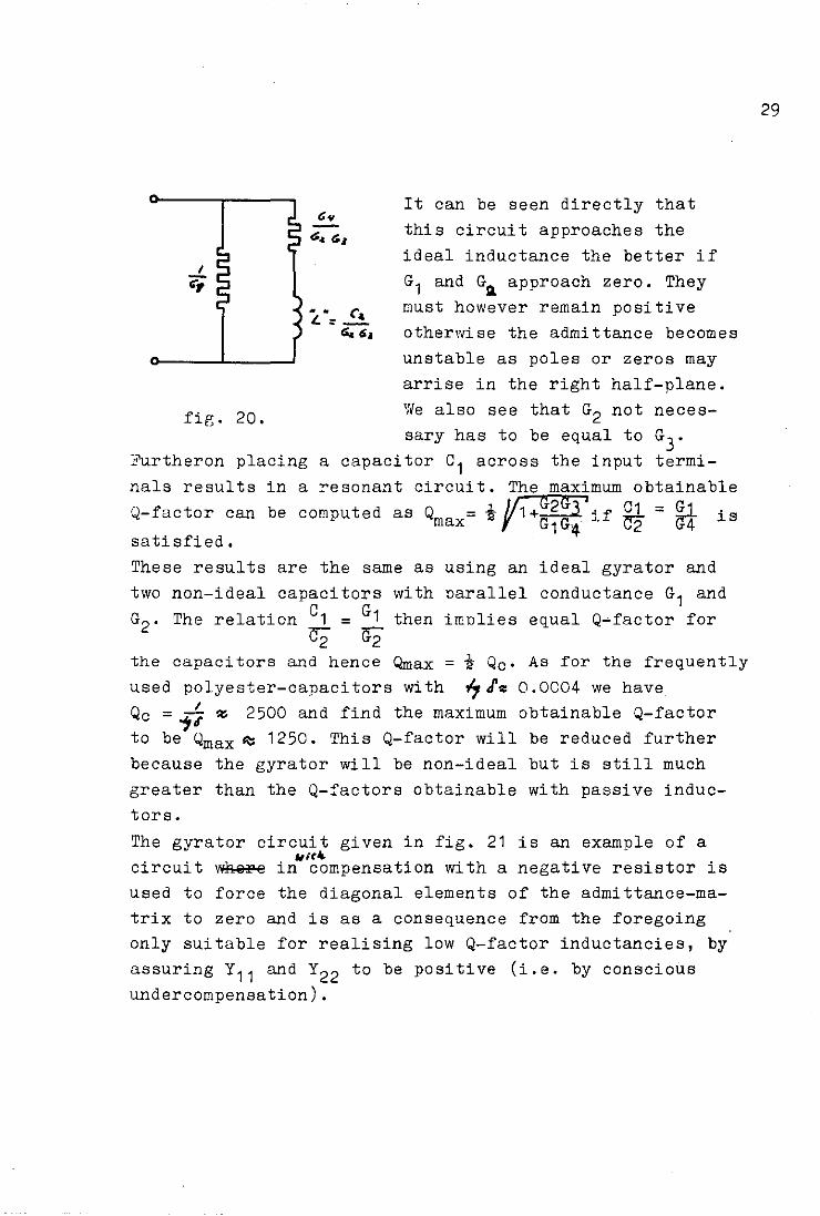
G4+pC2 The equivalent circuit for this admittance is given in

fig.20.

28

v

v

•• C i. =_~

Go 6,

It can be seen directly that this circuit approaches the

ideal inductance the better if G1 and Ga approach zero. They

must however remain positive otherwi se the admi ttance becomes unstable as poles or zeros may

arrise in the right half-plane.

f " 20 We also see that G2 not neces-~e· .

sary has to be equal to G3. Furtheron placing a capacitor C1 across the input termi­

nals results in a resonant circuit. The maximum obtainable

f G2G3 i G Q-factor can be computed as Qma = t l+G G . U Q1 = tl is x 1 4 C2 G4

satisfied.

These results are the same as using an ideal gyrator and

non-ideal capacitors with parallel conductance G1 and

The relation °1 = G1 then implies equal Q-factor for C2 G2

the capacitors and hence Qmax = t Qc. As for the frequently

used polyester-capacitors with 7'= 0.0004 we have Qc = 7~ ~ 2500 and find the maximum obtainable Q-factor to be Qmax ~ 1250. This Q-factor will be reduced further because the gyrator will be non-ideal but is still much

greater than the Q-factors obtainable with passive induc­tors.

The gyrator circuit given in fig. 21 is an example of a "rc ..

circuit \~ in compensation with a negative resistor is used to force the diagonal elements of the admittance-ma­trix to zero and is as a consequence from the foregoing only suitable for realising low Q-factor inductancies, by assuring Y11 and Y22 to be positive (i.e. by conscious undercompensation).

29

1

l'

2 A better circuit can be obtained from this one if the negative resistor is replaced by a feed-back loop as depicted in fig.22.

This results in an admittance-

2' matrix

f 0 6, 1 b1 -= fig. 21 • ,~slG&. t;,,,,,,~

-6-~ Nsf" H7ii,

If furtheron S/G2 » 1 this becomes

(~1 :: l-:. G, 1 r"t:J&.1

The latter shows that Y22 is always positive and can be made small enough by taking S sufficiently large and at

the same time G2 may be put to zero.

Because of the finite input imnedance of T1 and T2 the value of Y11 will not be exactly zero but can be made

small enough.

1 o---T-------------------~--------------~

r---~--_o2' 2o---~

, 1 O---~----------------4_ __________________ ~ fig. 22.

•

A suitable practical circuit can be obtained from fig. 22 by rearranging its nullator-norato~ equivalent so as to .. produce a circuit with operational amplifiers instead of the given transistors. With the nullator-norator equiva­lence [~] of the ideal transistor and operational ampli­fier given in fig. 23 this step is indicated in fig. 24.

30

1

2

l'

From the last scheme in this fig. we obtain the practical

circuit of fig. 25 as was first given by Riordan (61 . B

c

fig. 23.

1

2 0-2'

l'

fig. 24.

1

2 2' o-+----.

fig. 25.

31

c: C

There remains however the important disadvantage for these circuits not being able to realise "floating" inductors

with one gyrator because of the galvanic coupling between in- and output-port. Some alternative gyrator circuits are based on the two current source equivalent depicted in fig. 26 as follows

from the decomposition of (30) in

10--..... ...---02

1'o---'------L---o2'

",fig. 26. fig. 27 • .. I

Mr Creemers of the TechnologicV Uni versi ty Eindhoven has designed and actually constructed a circulator circuit

with voltage controlled current sources given in fig. 27. Connecting a capacitor between the nodes 2 and 3 will give a floating inductance between node 1 and 2. However this circuit can become instable too if the admittances G1 , G2 and G3 are different

At last the circuit of fig.

be used as a circulator and tage as the one in fig. 27,

from each other.

28 as given bij Keen [1] can (/.Is­

suffers from the sameYadvan-however the large gain of the

amplifiers used in this structure assures its behaviour almost completely to be determined by the value of the

resistors, wich can be made sufficiently accurate to guarantee stable operation for Q-factors up to 500.

32

~ 2'

fig. 28.

All.resistors

~ value R • .... " ...

33

3.3 Active synthesis using frequency dependent negative resistors[o

Consider the transmissionmatrix of an LCR two-Dort with Darameters A, B, C and D. The voltage transferfunction of

this two-nDrt given by A is an irrmitance ratio and does not change when the admi ttancies in the network are scaled wi th a certain factor. Thi s p.)in t opens the possi bi 11 ty to

remove inductances by scaling all admittancies in the LCR tv/o port with a factor p.

1 In that case we find the general admittance Y=G+pC+ nL to be changed to y1 = pG +p2C + t . This implies that a con­

ductance G will be transformed to a capacitance pG and an inductance p1 will be transformed to a conductance t . However a capacitance pC will lead to an admittance p2c being a frequency dependent negative resistor (FDNR) for

p = j'-l. Hence we need an active circuit to realise the

?DlIR and Ul,e these elements together with resistors and

capacitors for realising the transformed network. Such an active FDlJR is given in fig. 29 together with its reDresenting symbol. Inherent to the configuration of thi s }'D!1R only grounded FDNR I S can be realised. Hence this substitution-method will only work properly if the origi­

nal network does not ce1ltain floating capacitors. As the mid-series type LCR filter fullfills this require­ment one tries to realise the passive filter in this form and afterwards derives the active circuit by the foregoing transformation.

1 ~--.-----I"'"

fig. 29,

34

As an example consider fig. 30, where

this transformation is shown in detail. A disadvantage of this realisation lies

in the output voltage going to zero as

w~ 0 • This is due to the finite in­put impedance of the operational ampli~

fiers in the FDNR. However if the orig­nal network is designed as to have only inductors in the generator-branch this will result in resistors in series with , the generator in the transformed net­

work thus leading to the right low fre­

quency response.

--

fig. 30.

As th~ FDNR is basically a positive immitance convertor (PIC) the resulting networks have an overall sensitivity comparable with other PIC-methods, wich are claimed to

be low. As a fact the FDNR is realised by means of a PIC as de­

picted in fig. 31. Here in the generalised PIC is a two­

port defined by the relations

V1=V2 (29)

I 1=H(p)I 2

A realisation for the PIC is shown in fig. 32 with

.. V1

11 k~:1

12 11

Z1

.. .. Z2 G V2 V

1

o o

fig.31. fig.32. 1 1

Taking Z1 (p)= pC1

' Z3(P)-PC2

' Z2(P)=R1 and Z4(P)=R2 gives:

H(p)= k p2 with k = C1C2R1R2

From (29) follows 11 = H(p) 12 hence connecting an ad-VI V2

mittance Y to the secondport results in an input admittance Y'n= H(p).y. Returning to fig. 31 we find Y. =kp2y =kp2G ~ ~n "

being a FDNR and the resulting schematic diagram becomes that of fig. 29. With these PIC's we can also simulate inductors directly

as can be seen from fig. 38, leading to an input-im­pedance Z=~ corresponding to an inductor "1" = ~. In fact only one capacitor is used in this PIC and if we would redraw the schematic diagram in fig. 33 in such a way that the nodes where to the capaCitor is connected would form the second port instead of 2_21 , the resulting circuit would appear to be the gyrator given in fig.2~ Therefore replacing inductors by gyrator-capacitor cir­cuits is equivalent to replacement by PIC's

1 1'''" 2 A floating inductor is in this case realised as shown in fig. 34 requiring

G the PIC's t~ .. have .",,.,.,nt ¥,...~ ~". ,. .. ."., exactly reciprocal

in order to avoid ]I ...

1 b lee

35

t • 3

I "_,, ,,_ul'l'Ircl 6.lravl'"". "'/~jo /l.t. l' 2'

~f""~tll'''; ''''-/1,,,1. fig.33 • .

-

fig. 34-.

no--rvv"~-....,o

L " ..c.'!

O~------------Q

In fig. 35 an example of this substitution method is depicted.

J

fig. 35.

The block with PICs performs a transformation as indicated by the following. Consider a resistive network Inth impedance-matrix Z con­nected to a block of PICs as given in fig. 35.

For the resistive network holds V= ZI with ~=(1.Jand I =!: .. ;')

The PI C s gi ve : 1.11,') ('!) "'" V'=Vand 1'- ~pI with V'= fI~' and 1'= /..,

Therefore 4 t .. /I ~ II,. 7.:r .. ,,1..; %:r ~ resulting in an impedance matrix for the nodes 1',2', •.. ,n' given by Z'=kpZ.

36

.1: kP , ,

v,.l, " v,,I,

V~ 1J,h N

0---- - - - --------0--- --------

v,;~ n' ~.

fig. 35.

Hence the network between these nodes is an inductive net­work with the same topological structure as the resistive network in wich every inductance Li has a value determined

,. lJIt'e

by Li=kRi with Ri being the corresponding Resist~ value in network N. As these PICs have basically a gyrator structure and per­form the same substitution, this method will result in the same low sensitivities as for the gyrator-capacitor substi­tution and in advantage over them they have the possibility to replace more inductors with less PICs on account of the above derivations. Furthermore for constructing floating inductors with gyrators, one needs a type with one common input- output node and untill now no such circuit is known

with a simplicity comparable with the above PIC-circuit. Hence we may conclude that the PIC-substitution is most favourable, leading to active networks with sensitivities comparable with those of the passive networks from wich they are derived, while only known passive synthesis me­thods are involved to design the active filter.

37

4. Active filters on synthesis basis.

The active filters considered in this section have the property that the impedance matrix of the embedded net­works can be derived from the original transferfunction by means of a general method in such a way that these former networks become realizable RC networks. The structures given in chapter 4.1, 4.2 and 4.4 can realize every stable rational transferfunction, where as the gyrator-RC structure in chapter 4.3 is limited to certain filter classes.

4.1 Negative Impedance Converter (NICl Synthesis.

One of the first available active filter structures given by Linvill uses a NIC in conjuction with two RC networks for realising transferfunctions. The basic configuration is depicted in fig. 36, in wich the cur­rent-inversion NIC is shown between the dotted lines.

,...-----------, I ,

I I I I

lot I I t; Na 'Rt R.,

. Nb I I I

I I I I

I I I ,

L _____________ J

fig. 36.

With k we find the chain-matrix of the NIC as

38

Wi th this structure

chain-matri~,the transferfunction of ths above is given by

b a Z21· Z21 (30)

b a Z11- k Z22

The realization of a given transferfunction proceeds as follows. Let H(p) be written as

H(p) = ~t~~ with N(p) and D(p) polynomials in p. As a first step devide the numerator and denominator of H(p) by an arbi­trary polynomial Q(p) with its zeros on the negative real axis and degree Q(p) equal to the maximum of the degree of N(p) or D(p). Hence

We now equate (30) and (31) resulting in

Z2~·Z2~ = ~(p) / Q(p)

Z1~-kZ2~ = D(p) / Q(p)

(32a)

(32b)

Here after D(p)/Q(p) is split up in rational fractions giving

Let the ~ be numbered in such a way that the first r

39

values of k)" are positive and the other N-r values are negative. Taking now ki = -kli _r for i) r, we can write (33) as

D(p) fJ .10 ,. ~1 J [f" .I" ]- ~ - -I. ~ Q1PT = r- of" P 'ft "".~ -..... .., />"'r. •• - r:q.~) Q.(,)

From (34) we see that D1(P) and D2(P) are realizable RC . Q1(P) Q2(P)

impedances because all k/" and l~ are positive. Therefore we can equate (34) and (32b) giving

Z11 b D1(P)

= Q1{P) (35 )

Z22 a D2(P)

= Q2 (p)

Furthermore (32a) can be written

K(p) N1 (p) QTpT = Q1{P) •

leading to N1 (p)

Q1 (p)

Z21 a = N2 (p) Q2{P)

(36)

as

40

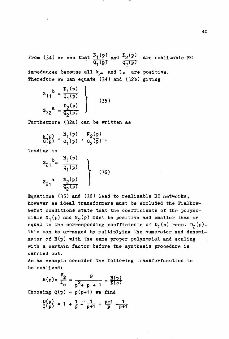
Equations (35) and (36) lead to realizable RC networks, however as ideal transformers must be excluded the Fialkow­Gerst conditions state that the coefficients of the polyno­mials N1 (p) and N2 (P) must be positive and smaller than or equal to the corresponding coefficients of D1 (p) resp. D2 (P). This can be arranged by multiplying the numerator and denomi­nator of H(p) with the same proper polynomial and scaling with a certain factor bsfore the synthesis procedure is carried out. As an example consider the following transferiunction to be reali zed:

V2 p N(11l H(p)= r ,. ,. mpr

o p2+ P + 1 Choosing Q(p) ,. p(p+1) we find

D(Pp

) • 1 1;:' 1 _ £±1. _ 1 ~ + p p+1 - p p+1

1 = p+1

Furthermore ~~pj can be split up in

N(p) _ P _ l2. 1 QTPT - p(p+1) - p • p+1

Hence we may identify Z21b= ~ = 1

1 p+1

(i.e. k=1)

This leads to the realization as given in fig. 37. The current source with parallel resistor can be changed ina voltage source with series resistor, giving a circuit with voltage transferfunction H(p).

,.---------,

t

,

, , l' ,

, L. _________ J

NIC

fig. 37.

,.._ .. _----. I 1 I

All resistors in Ohms, capacitors in ~rads.

4.1.1 Sensitivity considerations for the Linvill synthesis.

From (30) we find the poles b a determined by Z11 - k Z22

D1 (p). D2 (p) Q1 (p) - k Q2(P) = 0

of the transfer function to be = O. With (35) this becomes

Therefore the poles follow from

41

Defining the polynomials A(p) = D1 (p) Q2(P)

and

we find (37) to become ~ ,.

p

= z:. 1l..,1' "" "' .. p

= =z:. 4...,,-", ..

42

A(p)- k B(p) = 2: (16..,_.11 ... ),"= ~ ," ... , .. :: O. "":;0 -~.

(38)

From (38) the coefficient sensitivity can be calculated as .....

S.J.. ,.. ./.4 - . c ..

Especially when a certain small en is obtained by substrac­ting large values for An and k bn , the resulting sensiti­vity s~n can become very large. If the poles of the trans­ferfunction to be realized are situated close to the j W -

axis, a small change of one of the coefficients of the de­nominator polynomial may result in right half plane poles and therefore the NIC synthesis may lead to a circuit ba­lancing on the edge of instability. There is however a degree of freedom in the choice of the polynomial Q(p) and one may expect that this polynomial 'can be taken in such a way that the pole sensitivity with res­pect to k can be minimised. Indeed, for even degree D(p), Horowitz [tl1 has given the conditions for the polynomial Q(p) as to minimise the pole­sensitivity for variation in the NIC k factor. The denominator polynomial of H(p) must be split up into

A?t "4 -, 7Jtj>J. 7T '1",IIIJ.t - :a., IT (t,.",,)' _;t,t 3.:> (J'; ai, "0 ~ 0

i. a/ ,:.,

The polynomial Q(p) then becomes ... ,4 't:i -,

<V~). I' 7! ~jf'"') 7f ~"'M . ,I:, '61

This procedure appears to be quite general as it can be applied in any case in wich the difference of two polyno­mials is involved where in one polynomial can vary with a constant factor. Calahan [101 has given a method to obtain Q(p) in another way in wich no such inhomogeneous system of equations is involved as with the Horowitz method.

43

In spite of this optimation procedure the Linvill synthesis is only applicable for low degree and low Q factor trans­ferfunctions. It has however given the first start for active filtersyn­thesis and gives insight in the problems that can be en­countered in these synthesis technics.

4.2 Synthesis method of Yaganisawa.

The structure given by Yaganisawa is depicted in fig. 38, and is also applicable to realize '. 'I'· rational trans­ferfunctionswith R-C elements and one current inversion NIC.

-I~

'2

E t Y1

~ t CINIC I :1'6

+

fig. 38.

The transferfunction of this circuit can be calculated as

H(p)

Following the same procsdure as in chapter 4.1 we find

~~Ej ~fEj (Y1-k Y2 ) H(p) = 1m" D~El-N~El +§ffi

= (Y3-k Y4}+(Y1-k Y2 ) Q p Q(p

From the above formula we equate

(40 )

In the partial fractions expansion of the left hand side of (40) we collect the fractions with positive residues to form Y1 and Y3 while the others from Y2 and Y4 • For Y1 etc. to be RC admittancies the degree of Q(p) nas to be one less than the maximum degree of N(p) or D(p) and again must have its zeros on the negative real axis. Then all admittances can be realized in a Foster parallel RC form and the synthesis is completed.

44

The sensitivity considerations are generally the same as those of the previous chapter as was shown by J.Schwant [H) As an example of this synthesis method consider again the

realisation of H(p) = P ( ) 2 wi th Q p = p+1. p +p+1

We find D(p2-N~p2 Q(p =

p2+1 _ ~ p+1 - p+1 - p+1 = Y3 -k Y4

00 Q p = p;1 =

Taking k=1 gives

Y1 = p;1 Y3= p+1

Y2 = 0 Y4= p!Y The final filter is given in fig. 39.

1 1 o-Ul.I1r---j

:l !

E 2 1 1 CINIC

k=1 2

fig. 39.

)

Recently, Ruprecht [I:] has given a synthesis method similar to the Yaganisawa method in wich the finite gain of the operational amplifiers as well as the generator output im­pedance is taken into account.

4.3 Synthesis with the gyrator as a two port (1/1.

a two port element

45

In this method the gyrator is used as loaded on both ports with Re networks as indicated in fig.40.

+ E

t Na

r-- r--

) ( Nb

fig. 40.

The transferfunction can be calculated as

v~

E

t +

Here in Rg is the gyrator resistance of the use~(~,rator. In order to realize the transferfunction H(p)= ~ with complex poles, it must be split up as follows: 1. Express D(p) as "/0

"If, ~ ~ ~ 7)(,,) '" If fJ>~tf") r~. 7l (1,,1,)

~. /-, ~ %

2. Determine Q(p)= /P.ll. 7lf;Hc;) 1[ (p~J,') 1&' i~,

3. H(p) follows as

H(p)= ~~~l/ ~~~l wi th N(p)

this H(p) and

'" N1 (p) .N2 (p)·

(41) results in

~ jf{p(',') e·.'

4i I. Tl.fi-"",) ,.,

(42)

Calahan [IJ J has shown that ths re sul ting Z 11 b be realizable RC immitances if the following fied.

a and Y22 will lemma is satis-

Lemma: Let the complex poles of H(p) be given by

;{C7C r P''') P = /Pi e 10/;11. ,,<: f" , 1

i1 ,2

46

Then y22a and Z11 b given in (42) are realizable

RC immitances if .... & >t ~ ~,'! r . 1='

This lemma puts a severe restriction on the realisation of higher-order transferfunctions, however any second and third order transferfunction is realizable as always ~1 ~ ir for stability reasons. Hence this implies that any higher order filter can always be realized with this method by cascading and isolating second or third order sections. For biquadratic and bicubic low-pass transferfunctions a more direct method can be followed as will be demonstrated below for the bicubic case.

I I Let H(p)= = -

From (41) follows F(p) =

As will be proven later on we can choose f1' so as to produce positive residues in (43). Splitting up k2 as k2 = k2

a + k2b we derive from (43)

a Rg Y22 =

The partial fraction form in (44) indeed realizability for Z11 b and y 22

a

47

(44)

guarantees the

Furthermore as depicted

b if Z11 and in fig. 41,

Y22a are realized the resulting y 21

a in the Cauer form

b and Z21 will

become b

Z21 = , Hence the transferfunction H(p) is realized except for a constant factor •

. , , , , , , , I .------0--;-----''------'--+--0

fig. 41.

In order to prove that k~ , k1 etc. can be made positive we express them in ~ andofwthe coefficients of F(p) leading to

k3 .-!-

k1 r~r)

= Nrr = IJrrA.

ho-I .!! k2 = - k ... = H tr4- II

Requiring all k to be positive then results in

Ff-rr) >0 } ho-I >0 (45)

Consider next the value ~ being

rt'-I)

As the Hurwitz condition for F(p) implies ~ < L we have Ft-f.) > 0

I .J. From the above relation follows that for ~ '>;; and /f'- '"

sufficiently small always ffor) > t!J can be realized. In this case both relations in (45) are satisfied and therefore all residues k are positive. This synthesis method will be demonstrated with the follo­wing example.

1 Let H(p) =

1 1 We find M = 2 and therefore try J

u= I > 11

This results in j=f-rj./, hence (45) is satisfied. Equation (43) gives with A=1

Ffp) "!"'IP·~I.I>~J ? I .. ..L _ _ -:-. r co h~ ____ .,.

p(p;l) />(1'''"') r p~' ,.

Taking Rg = 1 this results with (44) in , ~

'Z,," :: p

A~...t- .. /. r /O~,

The Cauer form for filter is depicted

a Y22 is in fig.

given in fig. 42 and the final 43.

% Rg=l

4 1 1 l~ 4 1 .. a ~2 -

fig. 42. fig. 43.

4.3.1 Sensitivities for the RC gyrator.two-port synthesis.

As in this synthesis procedure the poles are determined by a sum of polynomials rather than a difference, the sensiti­vities are smaller than those of the NIC type realisations and comparable with those of passive filters.

48

The procedure of chapter 4.3, as proved by Calahan, gives the lowest possible sensitivity with respect to variations in gyrator resistance for every possible decomposition. Furthermore the circuit is always stable for any element value in contrast with the NIC structure.

4.4 Synthesis with PICs by the Antoniou method.

Recently Antoniou[/~1 has given a synthesis method able to realize every rational transferfunction with PICs and in­verting amplifiers. The main advantage of this synthesis method lies in the simpl'city of the realization and cal­culation of the element values. In realising a voltage transferfunction H(p), Antoniou proceeds as follows: .. Let H(p)=

A • ., .,,tJ ~ .. - .,.. ",. p

~.",I'~ ... ~"",J>-

Consider furthermore the voltage transferfunction of a parallel connection of two networks Na and Nb ' given by

49

(46 )

V _ ,., (_ ,~,C) ~ ~- 11,4)

E = -;;: = r"A"j ~ (!,u 4 ) • (47)

Then (47) implies that H(p) in (46) can be formally realized by the parallel connection of Na and Nb with

} (48a)

and

The network Na corresponding to (48a) is realized as depicted in fig. 44 in wich a switch is positioned to the node labeled "_" if the a i corresponding to the connected element is nega­tive or to the node labeled "+" if the concerned a i is posi­tive.

The network Nb with Y- parameters given in (48b) is rea­lized by a network Nc in cascade with a PIC with current transfer ratio 1: k1P2 as depicted in fig. 45.

/;

The PIC gives V .. = /I .. I

I 1

2A. I.'I'~ r. '

fig. 44.

• 2 1:k,p I2

I~c I D I +

fig. 45.

(49)

(50)

From (49) and (50) we find for the network Nb 'I,. ~uC' P,,, ,,?14 C' ~

.T". "'I'~ 'Y"e /I, , "'/I~"" c ~ resulting in

'Y"" -k'I''' 'Y. ,e

,. ... J= .J,,.C , .. c

)

50

Together with (48b) this gives

- rAI<": Aa II, 4.... -.-,t.

} ::r. ~ r. p'" ---- .. Z; ,b

1 ... t = 4& -4. .,. 6.... --.t (51 ) X ~;r,,*~--" :;i;, ,b

Being arrived at this stage we can repeat the whole proce­dure starting with equations (51), at each step reducing the degree of H(p) with two untill all coefficients are realized. Because of the nature of the above synthesis all denomi­nator coefficients are realized as a sum of maximally two element values. This implies low coefficient sensitivity as to the composing element values and zero coefficient sensitivity for all non composing elements. However the same remarks apply as given in section 3 concerning the possibility that slight changes in the element values may cause instability if high-Q poles are realized.

4.4.1 Special cases for the Antoniou method.

51

If second or fourth order low-pass filters are to be de­signed with all transmission zeros at p=~ , the Antoniou procedure can be modified as to result in a circuit with less capacitors. In this case the denominator polynomial can be split up as follows:

For degree 4 4.I"H'I'J~C'l't" 4#/,~Q.~fol ",/,C/,"Ilf,) 0~" /,(/,"IfAJ]ja",

For degree 2 fl.' ..... '/'" c2.t" ~/ ... 1'(,b .. .r,)J flQ

This leads to the realisation as depicted in fig. 46.

4th order low-pass 2nd order low-pass fig. 46.

Furthermore every second order transfer function may be realized with one PIC with current transfer ratio 1: kp as given in fig. 47, from wich the transferfunction can be derived as

+ Erv

a,

4.1'~ "'(4,1' .. "'. '. p'" A, I' .. 6~

1..-••

fig. 47.

A negative value for a 1 can be handled in the same way as with the original Antoniou procedure.

52

As proved by the au thor [ISJ the Q factor rea11 zed with thi s circuit is in first approximation independent of the band­width of the operational amplifiers in the used PIC circuit of fig 32 ,and 11mi ted to Q Z II; in wich Ao is the DC open-loop amplifier gain. Therefore this method enables very high Q factors to be realized,insensitive to tempera­ture variations as these mainly cause changes in the ampli­fier bandwidth. As the circuit of fig. 47 is also stable for all element values it is very suitable for synthesis by cascading second

order sections. Another interesting feature for this configuration is the possibility to realize second order transferfunctions with zero Q factor sensitivity with respect to changes in the current transfer ratio of the PIC. Consider for example the circuit of fig. 48 with transfer­function

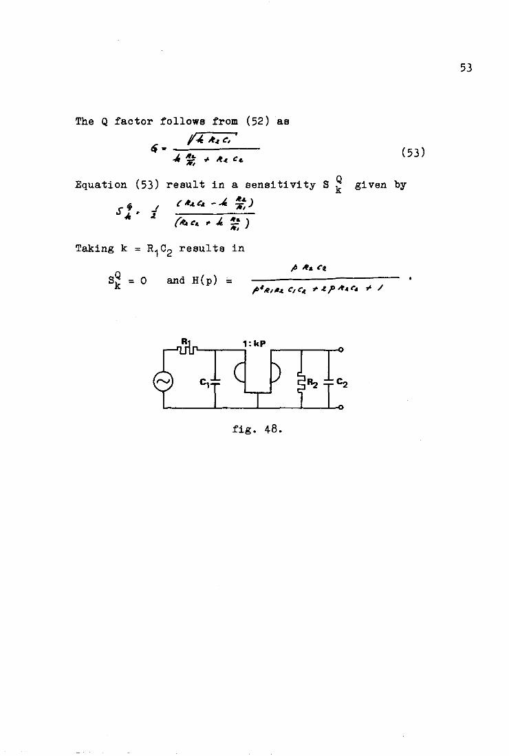
The Q (52) as factor follows from

!.Ie .t~ c, ' ~. ---:----

~ ~ of' .t. c& (53)

Equation (53) result in a sensitivity S ~ given by

sl· f 0 ... 4 --' }~)

(If.t c. ~ .. ~) 10,

and H(p) =

,: kP ~,---, r--.---~

fig. 48.

53

5. Cascade synthesis with second order sections.

In this section a survey will be given over ~ various active second order transferfunction realisations wich are frequently used in cascade synthesis. Some of these structures can only realise low-pass or high-pass filters, where as other ones are only suitable for low Q-factor transferfunctions. However these circuits use less compo­nents as compared with the more general types and may therefore be prefered in some cases.

5.1 Second and third order low-pass Fj~lbrant filters.

A. Second order design equations. Let the transferfunction be given by

H(p)=

Then the realisation is given in fig. 49 in wich the element values are to be determined as follows

1. Choose a value k being the capacitance ratio of C1 and C2 •

2. Calculate a, b and c from

3.

a = c =

With the

R1 = R2 =

"" -~ .... X

values 1

blc

in pnt. 2 the elements become

C1 = a

C2 = c

The gain A is determined by

//= .t 0.,.74) _;' /,N,{4-The above realisation results in minimum coefficient sensitivity as to variations in amplifier gain given by

I' .t hi Ir- ., S I· Trl" 'tI.J - 7 •

54

From this formula it" can be seen that k must be taken as large as possible, while small;9 (i.e. high Q fac­tor) results in high values for S: Therefore this circuit is only applicable in low Q fac­tor transferfunctions.

c,

Ax + ". E QI O~-----------------L--________ ~o

fig. 49.

High-pass filters can be realized by the frequency transformation ,. .... '; • This results in the following impedance transformation:

Impedance

Impedance / -,be

--+ Impedance

Impedance

equations 1

B. Third order design

Let H(p) = 3 12 Kp +Lp +Mp+1 = FtPT

/ -"tiC

The realization is given in fig. 50 in wich the element values are determined as follows:

k 1. Choose a; with "" < c1i <;;r in wich - VO is the real

pole of H(p). The other two poles are supposed to be complex. Choose o:r. in such a way that cr.. ')-01; and

r~-/rr,) O&(-hr..., / ;> 0 •

2. Express ting in

3. The element values then follow as

fractions resul­-to. - -/?"r.e

55

..1:1 ?/C" ... /e,) (

R1= ..4 .. (./c • ., ~,) C1= 11"1 .Ie,

I ../cd> R2= .Jr. ,".4, C2=

I -1:", - -" .. R3= ~.k .. --'.e. C3= -.,-.. The above procedure can be proved to result in positive element values. In order to achieve minimum coefficient sensitivity the values of tfj and trot must be taken as small as possible. For high-pass filters the same considerations hold as in sub A. Again as a consequence of the relative large sen­sitivities this filtertype is only suitable for low Q-fac­tor realizations.

[L-~--I /x

o_IL-Ci

__ 1--1....-('&_--00 fig. 50.

5.2 Active realizations of second order notch filters with a modified Twin-T network.

In these structures a Twin-T filter is used to produce transmission zeros on the J~ -axis. Depending on the behaviour of H(p) at t>,., () and I> = 00 two different structures must be used for the realization, as given in fig. 51. Together with a frequency transformation the given net­works can realize any second degree notch filter. However in order to produce the transmission zeros sufficiently accurate, the element values of the Twin-T must be care­fully realized i.e. with tolerances 0.1%.

56

H(p)=

fig. 51.

With these circuits Q factors up to 10 can be achieved for element tolerance of about 1%.

5.3 Active filters employing negative feedback.

Consider the circuit given in fig. 52.

t E

fig. 52.

3

• V

Supposing the voltage transferfunction of Na and Nb in the configuration of fig. 53 to be given by Ha and Hb resp. we find the transferfunction of the circuit in fig. 52 to become

57

1

I~ • E 3

fig. 53.

The poles of R(p) are therefore determined by the zeros of Rb • As a bridged-T network is able to realize complex zeros we can use this type of network for realizing Rb • Then Na has to be a suitable network with the same poles as for

Nb • The eynthesis proceeds as follows.

Let R(p) be given by R(p)= k~IEj in wich k is a suitable

factor to be determined later on. Devide numerator and denominator of R(p) by a second degree polynomial Q(p) with its zeros on the negative real axis and all coefficients larger than or equal to the corresponding coefficients of D(p). This results in

/)(p) -Q(P} (55)

Equating numerator and denominator of (54) and (55) gives

HI. .. DCp} - (56a) 0(,.)

DCp} _..4 IVCp)

H. = ( 56b) ~(P)

58

In (56a) we can make a suitable choice for Q(p) so as to produce a simple network for Hb such as the earlier mentioned bridged-T network. Here after we can take k in (56b) small enough to result in a realizable RC net­work. At last the transferfunctions in (56a) and (56b) are realized with RC-networks, wich networks are then inter­connected according to fig. 52. As an example consider the realization of

kp H(p)= -"2r--

p +p+1

Taking Q(p) = p2+4p+1 and k=i we find

Hb= )22+)2+1 p2+4P+1

and H :: )22 +EL2 +1 a l+4P+1

The realizations of Ha and Hb are given in fig. 54.

0 ~

.J TVf

~ .I 0 0 0

AI. fig. 54.

The final network is depicted in

fig. 55.

'VV' ~"

fig.

t

~' ~ 1

9

Alb

55.

I

~ o

J

59

As the poles of the transferfunction are given by the zeros of Hb the sensitivities to element variations are small. Furthermore the polynomial Q(p) can be chosen in such a way as to minimise the pole sensitivity, however this possibility is not further investigated.

5.4 Second order filters with PICs.

As a last example of second order filters we mentione the circuit given in chapter 4.4.1 with one PIC having a current transfer ratio of 1:kp. As stated there this filter type has a lot of advantages over other realiza­tions for instance its simplicity, stability and the possibility to realize high Q-factors. Together with the minor influence of the operational amplifier band­width and the available sensitivity compensation for variations in the PIC current transfer ratio, this circuit will probably be the most suitable for second degree transferfunction realization.

60

APPENDIX

General formulas for the elliptic approximation.

Before deriving these formulas we consider again the Chebychev approximation that can be written in another way as

iP (;u.)= Ctn (m4<.)} ",. I) l) .....

Jl. = c.r.I __ (1 )

61

From these formulas one can see that the range (J ~ Jl. ~ /

corresponds to ~ ~ '" ~ 0 ,overlooking the periodicity in U •

In the given range for It. the function It-u.) will pass through ~ quarter periods varying between +1 and -1. Hence ~(A) will have equiripple behaviour in the pass­band 06.Jl. ~ / due to the periodicity of cos ( .. u) •

In transition and stopband however we have ft» / leading to complex U . As cos (~«) is not periodic for complex values of its argument, the function ~~) won't be perio­dic either and therefore cannot have an equiripple stop­band behaviour. Because we are interested in equiripple in the passband as well as in the stopband, we will have to construct a transformation comparable with (1) having double periodic properties wich are known as elliptic functions. These functions are defined by means of elliptic integrals as indicated below. Let E(x,k) be the value of the incomplete elliptic inte­gral of the first kind with argument x and modul~ k given by

(2 )

Furthermore the complete elliptic integral of the first kind denoted by K(k) is defined by

If no confusion can arrise K(k) is shortly written as K. The complementary complete elliptic integral of the first kind is defined by

"1 ~ k': £ f '?, "') • /;;:;===#=::==7."':'"

" fi-tv (/-.J:'~i·) (4)

wi th -Ie ' .. JlI-.J:~':'" being called the complementary modulus. From (2) we can formally express the value of x in the value of M. E (", I.) by wri ting

In this way (5) and the relation are defining inverse relations. Its therefore custummaxy to denote from (4)

.u. J?o-'(~,4)

Comparing (6) and (7) we have ~ cd

'U. s:n-' ('X) 4) r E tfo, 4) ~ / • d fQ-t<j (I-"'~t~)

(6 )

(8)

The function 4->0(,",1.) defined by (5) and (8) is called

the Jacobi elliptic sine function. This function can be proved to be double-periodic with periods -u. =4l( and u. =2jj(' where l( and l{' are given by (3)

and (4) resulting in

Ao-I (<<"flJr) -Ie). 4-J.t. bt,-,) J ..;.., ("'~~ilr~4J= __ ("'J.f) (9)

Furthermore we have from (3)

/-( = C /", Ie) =- ,..-' (", ~ )

and therefore #& (k, 1..) ,. 1 (10)

From (8) we also find

4>-0-'((},~):. 0 leading to _tP,.Ie} = 0 (11)

If ~ is augmented by a half period 2~ or jk' we have

A'>\ r'&f.';.t Ir, Ie) = - '"'" (-ti, ')

4'>-& (M.--jJr;IcJ- 1 (12) ..k ht t"" k)

Taking k=O in (8) we get >r

'f- / rP __ ~;";'(:I<) '" ~-Ibc) ",.- fIC,O)· ,= --

" JI,--t~ resulting in hot.""),, ~ I,.) (13)

Relation (13) clearly shows the periodicity of -#I. 11t:) 4)

for the special case k=O. The other Jacobi elliptic functions are defined by

c-n (-u, Ie.).. j!1- ;:-..'tU, ,;,

d,n. ("'I J.) =- 1I,-..k·"...·(U,-,)

and in general if p, q, r are any three of the letters s, c, d, n

7>'1. [-u, ')= ,tJl"tu,4) 'l-r(u,.Ie) provided that when two letters

are the same the corresponding function is equal to 1.

/ ""-s ('", ') ". .Ie

PI1/"" ) Thus

From (9), ( 11) and (12) we find

A>f. (r.,( Jr,.Ie) = 0 -frt..r = :t ", I,.t, .•.. I

and 4>1 (;/Ir'.;s . .L,jIr: I.) .. -ffl f;/Ir;.I:) ~ .l F>t.(o,")

leading to the pole zero pattern of A>f. (-Uric) as given in fig. 1.

r,., fCC)

)( x

fig. 1.

:x

)(

o

x

pole-zero pattern

of -ml"",4)

In this figure the shaded part is repeated periodically through the U - plane.

Derivation of the characteristic function.

In the elliptic approximation we use in comparison with (1)

As ..-ha(u • ..I.J in (14) is double-periodic in U. , we may expect that it will be possible to choose ($(.n.) in such a way that both pass-.and stopband will have equiripple behaviour. In order to find this relation we will examine closer equation (14).

This equation transforms the posi ti ve real.J1. -axis in the edges of a rectangle in theu -plane by the following way. The range O~Jl..$Q leads with (14) to o~ hr.(~.-4:).,;/>

or 0, -u ~ k

Hence o'..I2$Q is mapped on O&M.(, J( in the'l<.-plane.

The range r.1c ~..12 ~~ lead s to / ~ Po. (4<,.I.:) ~ i ( 15 )

From (12) we have . I /

-- ('tr~J ~,~)" ..4 1'Mff/j-4)

Taking 'Ir. I( give s --;..{ft,4J = p., (Ir) 4:) ,,? , hence

This leads together with

Therefore ric 4..Jl ~ if the It -plane.

The range ,z ~ A. ~ cD

/ .;[ ~ A-.. Co<,~) ~ oD

Again from (12) we have

I

(15) to

leads to

-4 A>. try; -i.)

in

(16 )

(17 )

From this follows JI1 h> (,.-, -'J. ~ ,.., (4""i"'~ ~ j = -1 , relating

the variables ..Jl" a ,.."(,,,,1.) and .1l&' 14 ,..,(,y~jlr: -4.) by

A, A. ... = / (18)

We already saw that 0 6 /I/' ~ k leads to 0 ~ ..12, .$ tr.i! with

.fl., lying in the passband. Thellfrom (18) follows that.1l .. -= =1'1e i'>r (/Y~jlr; 1.) = ..12: varies as required by

(16) from a to of> for the same interval of"".-, leading

to frequencies lying in the stopband. Hence frequencies

.fi., and.1l~ mapped on the '" -plane verti cal above each other on the lines 7_("')=0 and X",,( .. ) = kl will be

related by (18).

On account of the above derivations, the upper left-half

p-plane is mapped on the shaded part of the It -plane as

shown in fig. 2 and is periodically repeated there.

/(

fig. 2.

Next we take

~(,y)~ L -+n (N", /.~) (19 )

The pole-zero pattern of ar{~) is the same as in fig. 1

if the 'U -plane is changed in the /'Ir -plane and k is

changed in L2; the periods thus become 'Ik •• ~Jr{ ,t.~) , see

(3), and .l/Ir.'" ~.i/r(PI-"" '} As a consequence of (19) along 7',.,(41)" 0 the function

66

j§{4I) will vary between +L and -L and along 7',..,I'1/)=k.' §f",)

varies between + ~ and 00 • Furtheron if we relate U in

(14) and? in (19) so that the distance between -U"" and '1-L= k equals m- times the length ..... L of a quarter

period in the V'-plane,while at the same time """"jlr'

cOincides with 4/3 j k.' , we can superimpose the corres-

ponding periodic parallelograms of.fL. and II For even -n however the point 'U~ I( would coincide with

~" s· .2.4-. (r.:;) hence making I" (-v)" 0 in this paint.

As the passband edge frequency JlPG rJc. is mapped to the

point ~. k this would imply that at this point 5£..f1...)

would become zero where as the right value has to be ± L.

This trouble can be overcome if the whole -V- -plane is

shifted over a distance ~ in the direction of - "~{-u) ,

before superimposing both planes.

The resulting pole-zero pattern j. s shown in fig. 3 for

n=3 and n=4. 7-(_) r ... I..,)

fig. 3.

..;.zulf" "..a. + />..4 " "

o A.ur ~ 11

xjH&"u

From fig. 3 we see that /V. [ ,.. .,.'"' ,. I!' 1'",) ] ~

4'1-'" e( ... ).!" /rt. '" o In '70

in order to produce the desired real "'--AT - axi sis concerned. As can be seen or I'JI is kL + d Ire '

Therefore from

from fig. 3 also for n odd resp.

(20 ) follows

/r' "l -

k

} (20 )

patterns as far as the

'k' f,t~;J must lead to 4/" i lr,. ,

even.

giving

(21)

Relation (21) is an important one in the design-procedure because it relates the three basic design parameters L, k and n in such a way that any two of them prescribe the third. The desired zeros of jr{J.L) now follow from (19) by

resulting in

Then (20) gives

Finally (14) results in

J'los· ~ rn [ : [JU- (O{"';], .J. ]

s= } (22)

With (22) we can construct the characteristic function as

with

and fiDS given by (22).

68

REFERENCES

[1J J.K. Skwirzynski "Design Theory and Data for Electrical Filters",

D.Van Nostrand Co.Ltd., London, 1965.

r. 2 J Abramowitz & Stegun: "Handbook of Mathematical Functions",

Dover Publ. Inc., New York, 1965.

t 3 J T. Fjallbrant:"Canonical Active RC Filters with a Low Transfer Function

Sensitivity", Ericsson Techn., 23, 1967, pp.211-238.

[ 4 1 H.J. Orchard "Inductorless filters", Electronics Letters, ~ ,

1966, pp. 224 - 225 •

[ 5 J H.J. Orchard "New gyrator circuits obtained by using nullors "

Electronics Letters, ~ , 1968, pp. 87 - 88 •

[ 6 ] R.H.S. Riordan "Simulated inductors using differential amplifiers ",

Electronics Letters, 2 , 1967, pp. 48 - 51 •

[ 7 ] A.W.Keen,J.L.Glover

and R.J. Harris: " Realisation of the circulator concept using

differential - input operational amplifiers"

ElectroniCS Letters, ~ , 1968, pp. 389 - 391 •

[ 8 ] L.T. Bruton

( 9 J I.M. Horowitz

[101 D.A. Calahan

" Network 9ransfer Functions using the concept of

frequency-dependent negative resistance 11 , IEEE Trans.

on Circuit Theory, CT-16, 1969, pp. 406 - 408 •

11 Optimization of Negative Impedance ConverA9;r'sion

Methods of Active RC Synthesis ", 1-$ Trans. on

Circuit Theory, CT-6 , 1959, pp. 296 - 303 •

" Notes on the Horowitz optimization procedure" ,IRE Trans.

on Circuit Theory, CT-7, 1960, pp. 352 - 354 •

(11] J. Schwant " Beitrage zur Synthese activer RC-Netzwerke ", Ph.D.

Thesis, University of Stuttgart, Germany, 1969.

[12J W. Rupprecht:" Synthese activer RC-Netzwerke unter Verwendung eines

Differenzverstarker", A.E.O'., ~, 1969, pp. 445 - 448 •

[13J D.A. Calahan:" Sensitivity Minimization in active RC synthesis ", IRE

Trans. on Circuit Theory, CT-9. 1962, pp. 38 - 42 •

[14] A.Antoniou:"Novel RC-Active-Network Synthesis using Generalized Immit­

tance Conve rters" ,IIEETrans .Circ. Theory, llll,1970,pp.212-217.

(15) VI.M.G.van Bokhoven:"High-~ active RC-Networks"; to be published.

----------- 0 ------------

Reports:

EINDHOVEN UNIVERSITY OF TECHNOLOGY THE NETHERLANDS

DEPARTMENT OF ELECTRICAL ENGINEERING

I) Dijk,J., Jeuken. M., -Maanders,E.J. AN ANTENNA FOR A SATELLITE COMMUNICATION GROUNDSTATION (Provisional Electrical Design) TH-report 68-E-01, March 1968. ISBN 90 6144 001 7.

2) Veefkind A., Blom J.H. and Rietjens L.H.Th.: THEORETICAL AND EXPERIMENTAL INVESTIGATION OF A NON-EQUILIBRIUM PLASMA IN A MHO CHANNEL TH-report 68-E-02, March 1968: submitted 'to the Symposium on a Magnetohydrodynamic '. Electrical Power Generation, Warsaw, Poland, 24-30 July, 1968. ISBN 90 6144 002 5

3) Boom, A.J.W. van den and Melis J.H.A.M.: A COMPARISON OF SOME PROCESS PARAMETER ESTIMATION SCHEMES TH-report 68-E-03, September 1968 ISBN 90 6144 003 3

4) Eykhoff, P., Ophey P.J.M. Severs J. and Oome J.O.M.: AN ELECTROLYTIC TANK FOR INSTRUCTIONAL PURPOSES REPRESENTING THE COMPLEX-FREQUENCY PLANF TH-report 68-E-04, September 1968 ISBN 90 6144 004 1

5) Vermij L. and Daalder J.E.: ENERGY BALANCE OF FUSING SILVER WIRES SURROUNDED BY AIR TH-report 68-E-05, November 1968. ISBN 90 6144 005 X

6) Houben J.W.M.A. and Massee P.: MHD POWER CONVERSION EMPLOYING LIQUID HETALS TH-report 69-E-06, February 1969. ISBN 90 6144 006 8

7) Heuvel, W.M.C. van den and Kersten W.F.J.: VOLTAGE MEASUREMENT IN CURRENT ZERO INVESTIGATIONS TH-report 69-E-07, September 1969. ISBN 90 6144 007 6

8) Vermij, L.: SELECTED BIBLIOGRAPHY OF FUSES TH-report 69-E-OS, September 1969. ISBN 90 6144 008 4

9) Westenberg, J.2.: SOME IDENTIFICATION SCHEMES FOR NON-LINEAR NOISY PROCESSES TH-report 69-E-09, December 1969. ISBN'90 6144 009 2

10) Koop, H.E.M., Dijk, J. and Maanders E.J.: ON CONICAL HORN ANTENNAS. TH-report 70-E-10, February 1970. ISBN 90 6144 010 6

11) Veefkind, A.: NON EQUILIBRIUM PHENOMENA IN A DISC-SHAPED MAGNETOHYDRODYNAMIC GENERATOR TH-report 70-E-11, March 1970. ISBN 90 6144 011 4

12) Jansen, J.K.M. Jeuken, M.E.J. and Lambrechtse, C.W.: THE SCALAR FEED TH report 70 E 12, December 1969. ISBN 90 6144 012 2

13) Teuling, D.J.A.: ELECTRONIC IMAGE MOTION COMPENSATION IN A PORTABLE TELEVISION CAMERA TH-report 70-E-13, 1970. ISBN 90 6144 013 0

14) Lorencin. M.: AUTOMATIC METEOR REFLECTIONS RECORDING EQUIPMENT. TH-report 70-E-14, November 1970. ISBN 90 6144 014 9

15) Smets, A.J.: THE INSTRUMENTAL VARIABLE METHOD AND RELATED IDENTIFICATION SCHEMES. TH-report 70-E-15. November 1970. ISBN 90 6144 015 7

Reports:

16) White, Jr. R.C.:

EINDHOVEN UNIVERSITY OF TECHNOLOGY THE NETHERLANDS

DEPARTMENT OF ELECTRICAL ENGINEERING

A SURVEY OF RANDOM METHODS FOR PARAMETER OPTIMATIZATION TH-report 70-E-16, February 1971. ISBN 90 6144 016 5

17) Talmon. J.L.: APPROXIMATED GAUSS-MARKOV ESTIMATORS AND RELATED SCHEMES TH-report 71-E-17, February 1971. ISBN 90 6144 017 3

18) Kalasek, V.: MEASUREMENT OF TIME CONSTANTS ON CASCADE D.C. ARC IN NITROGEN TH-report 71-E-18, February 1971. ISBN 90 6144 018 I

19) Hosselet, L.M.L.F.: OZONBILDUNG MITTELS ELEKTRISCHER ENTLADUNGEN TH-report 71-E-19, March 1971. ISBN 90 6144 019 X

20) Arts, M.G.J.: ON THE INSTANTANEOUS MEASUREMENT OF BLOODFLOW BY ULTRASONIC MEANS TH-report 71-E-20, May 1971. ISBN 90 6144 020 3

21) Roer, Th.G. van de: NON-ISO THERMAL ANALYSIS OF CARRIER WAVES IN A SEMICONDUCTOR TH-report 71-E-2I, August 1971. ISBN 90 6144 021 I

22) Jeuken, P.J. Huber, C. and Mulders, C.E.: SENSING INERTIAL ROTATION WITH TUNING FORKS TH-report 71-E-22, September 1971. ISBN 906144022 X

23) Dijk, J. and Maanders E.J.: APERTURE BLOCKING IN CASSEGRAIN ANTENNA SYSTEMS. A REVIEW TH-report 71-E-23, September 1971. ISBN 90 6144 023 8 (In preparation)

24) Kregting, J. and White, Jr. R.C.: ADAPTIVE RANDOM SEARCH. TH-report 71-E-24, October 1971. ISBN 90 6144 024 6 (In preparation)