Embed Size (px)
Citation preview
Contents
• Clustered data
– What is it?
– How does it happen?
– What’s the problem?
• Robust estimators
• Generalized estimating equations
• Multilevel models
• Longitudinal multilevel models
Clustered data
– What is it?
– How does it happen?
– What’s the problem?

What is Clustered Data?
• Where cases are related – Lots of names
• Non-independence
• Dependency
• Autocorrelation
• Clustered
• Multilevel
• All statistical tests assume independence – If I know something about person 1
• That should not tell me anything about person 2
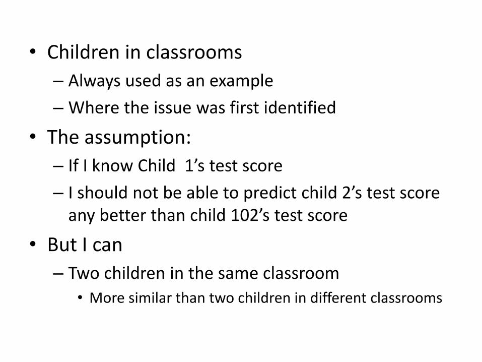
• Children in classrooms
– Always used as an example
– Where the issue was first identified
• The assumption:
– If I know Child 1’s test score
– I should not be able to predict child 2’s test score any better than child 102’s test score
• But I can
– Two children in the same classroom
• More similar than two children in different classrooms
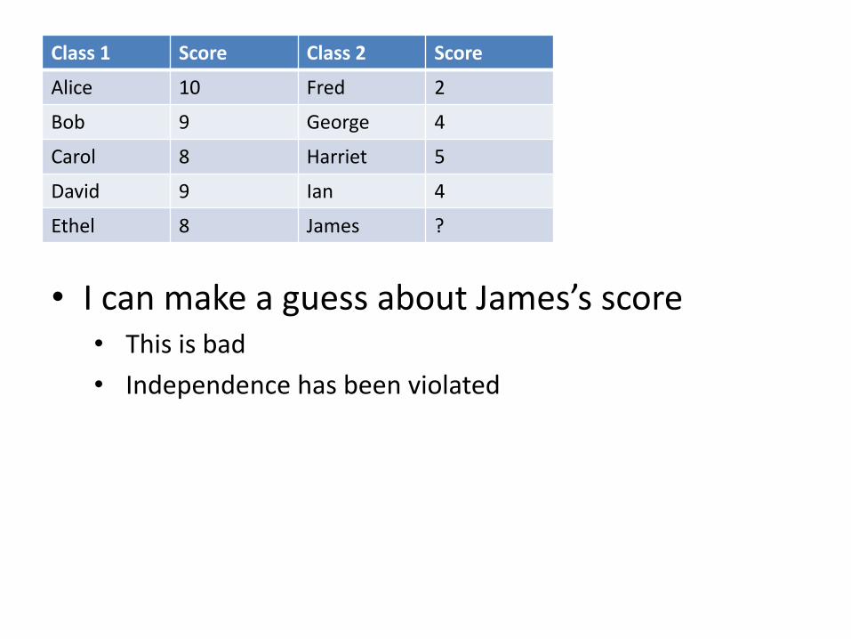
Class 1 Score Class 2 Score
Alice 10 Fred 2
Bob 9 George 4
Carol 8 Harriet 5
David 9 Ian 4
Ethel 8 James ?
• I can make a guess about James’s score • This is bad
• Independence has been violated
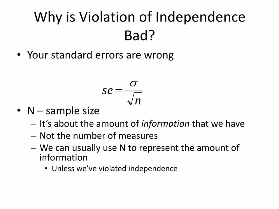
Why is Violation of Independence Bad?
• Your standard errors are wrong
• N – sample size – It’s about the amount of information that we have – Not the number of measures – We can usually use N to represent the amount of
information • Unless we’ve violated independence
nse

• 100 classrooms – 1 child sampled from each classroom
– N = 100
• Sample a second child from classroom 1 – There is non-independence
– Child 2 from classroom 1 does not provide as much information as Child 1 from classroom 101
• Child 3 from classroom 1 provides less information – Child 101 from classroom 1 – even less
– Child 1002 from classroom 1 – even less

The Intra Class Correlation
• Intraclass correlation (ICC)
– Same thing, used in lots of places
– Confusing
– In SPSS: Analyze, Scale, Reliability, Statistics,
• ICC is an option
• These are not the ICCs we are looking for
• We’ll come to calculation of ICC later

• Formula for intra-class correlation
• Where – M is the mean number of individuals per cluster – SSW – Sum of squares within groups (from anova) – SST – total sum of squares (from anova)
• (Very easy to calculate in Stata) • (Assumes equal sized groups, but it’s close
enough)
SST
SSW
M
MICC
1
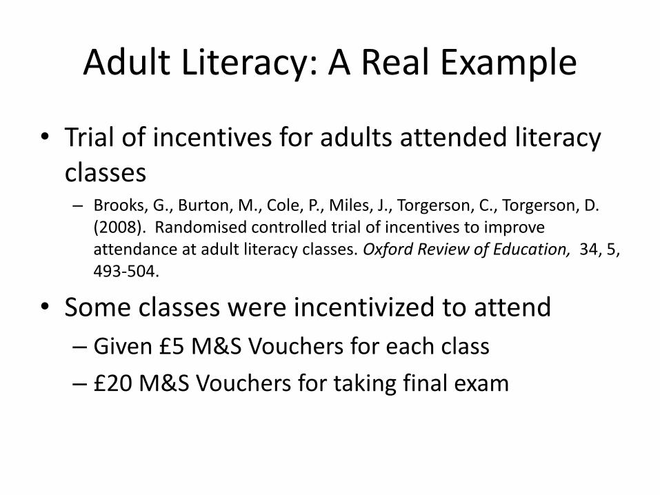
Adult Literacy: A Real Example
• Trial of incentives for adults attended literacy classes – Brooks, G., Burton, M., Cole, P., Miles, J., Torgerson, C., Torgerson, D.
(2008). Randomised controlled trial of incentives to improve attendance at adult literacy classes. Oxford Review of Education, 34, 5, 493-504.
• Some classes were incentivized to attend
– Given £5 M&S Vouchers for each class
– £20 M&S Vouchers for taking final exam

• Adults were in randomized by classroom
– We can’t randomize individually
• (which would remove the problem)
• Data are in ‘adult literacy.sav’
– Variables:
– Group: Group assigned to (not given to analyst – i.e. me)
– Classid: Class
– Sessions: Number of sessions attended (outcome)
– Postscore: Final score (outcome)
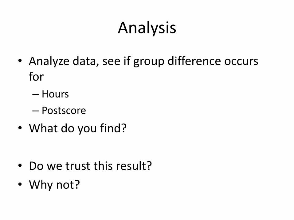
Analysis
• Analyze data, see if group difference occurs for
– Hours
– Postscore
• What do you find?
• Do we trust this result?
• Why not?

Violation of Independence
• It’s likely that we’ve violated independence
– Calculate the ICC
– …
Violation of Independence
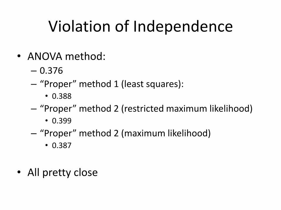
• ANOVA method: – 0.376
– “Proper” method 1 (least squares): • 0.388
– “Proper” method 2 (restricted maximum likelihood) • 0.399
– “Proper” method 2 (maximum likelihood) • 0.387
• All pretty close
Violation of Independence
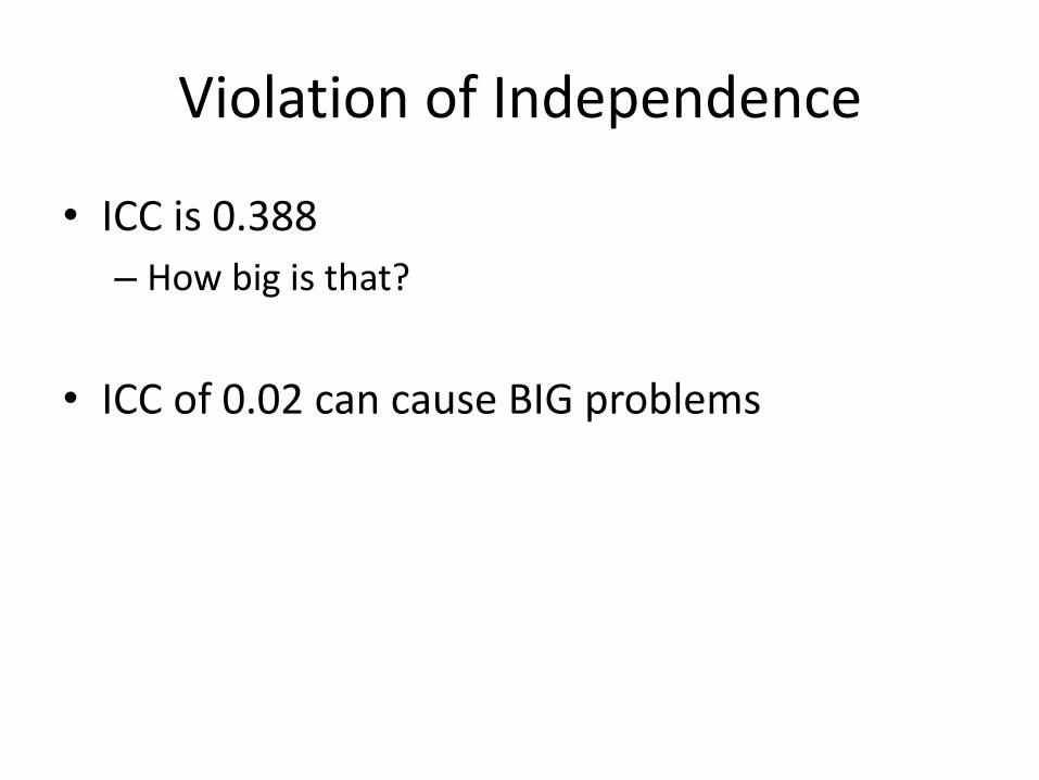
• ICC is 0.388
– How big is that?
• ICC of 0.02 can cause BIG problems
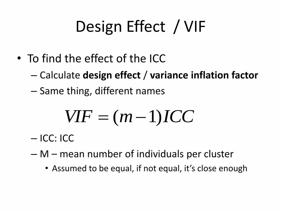
Design Effect / VIF
• To find the effect of the ICC
– Calculate design effect / variance inflation factor
– Same thing, different names
– ICC: ICC
– M – mean number of individuals per cluster
• Assumed to be equal, if not equal, it’s close enough
ICCmVIF )1(

• Tells you: – How much you have overestimated your sample
size by
• Calculate for our data:
• Our sample size was 152 – Our effective sample size was 152/3.06 = 49.7
06.3
38.0)128/152(1
)1(1
VIF
VIF
ICCmVIF
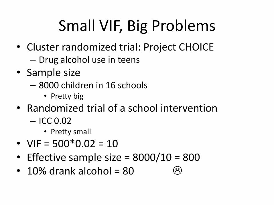
Small VIF, Big Problems • Cluster randomized trial: Project CHOICE
– Drug alcohol use in teens
• Sample size – 8000 children in 16 schools
• Pretty big
• Randomized trial of a school intervention – ICC 0.02
• Pretty small
• VIF = 500*0.02 = 10 • Effective sample size = 8000/10 = 800 • 10% drank alcohol = 80

Back to Our Data
• (Optional bit coming up)
• Standard error was 0.504 – Calculated with naïve sample size
• Standard deviation of parameter – SD = SE * sqrt(N)
– SD = 0.504*sqrt(152) = 6.21
– Corrected SE = 6.21 / sqrt(49.7) = 0.88
– t = est / se = 1.405 / 0.88 = 1.59 • NOT SIGNIFICANT
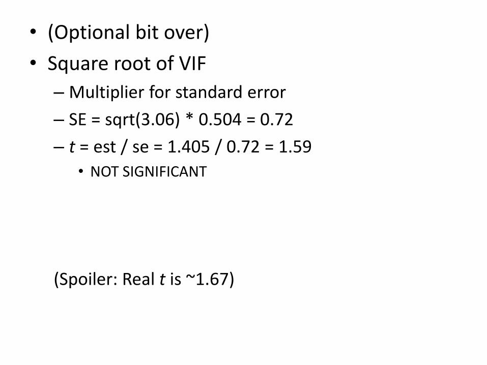
• (Optional bit over)
• Square root of VIF
– Multiplier for standard error
– SE = sqrt(3.06) * 0.504 = 0.72
– t = est / se = 1.405 / 0.72 = 1.59
• NOT SIGNIFICANT
(Spoiler: Real t is ~1.67)
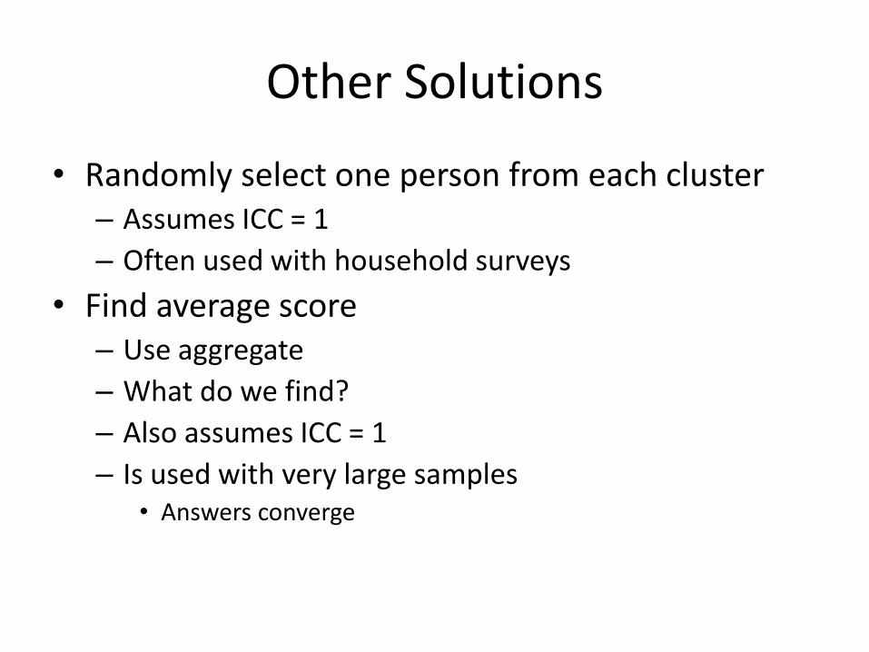
Other Solutions
• Randomly select one person from each cluster – Assumes ICC = 1
– Often used with household surveys
• Find average score – Use aggregate
– What do we find?
– Also assumes ICC = 1
– Is used with very large samples • Answers converge

An Aside on Psychometrics
• We give people psychometric tests
• We take many measures from one individual – That’s just like taking lots of children from each
classroom
• We add up the score (equivalent of taking the average) – Analyze each person with one score
• We calculate Cronbach’s alpha – This is an ICC

• We use the Spearman Brown Prophecy formula
– Longer questionnaires are more reliable
– But twice as many questions is not twice as good
– We don’t need to average, we can use items
• We call this factor analysis / structural equation modeling
)1(1*
N
N
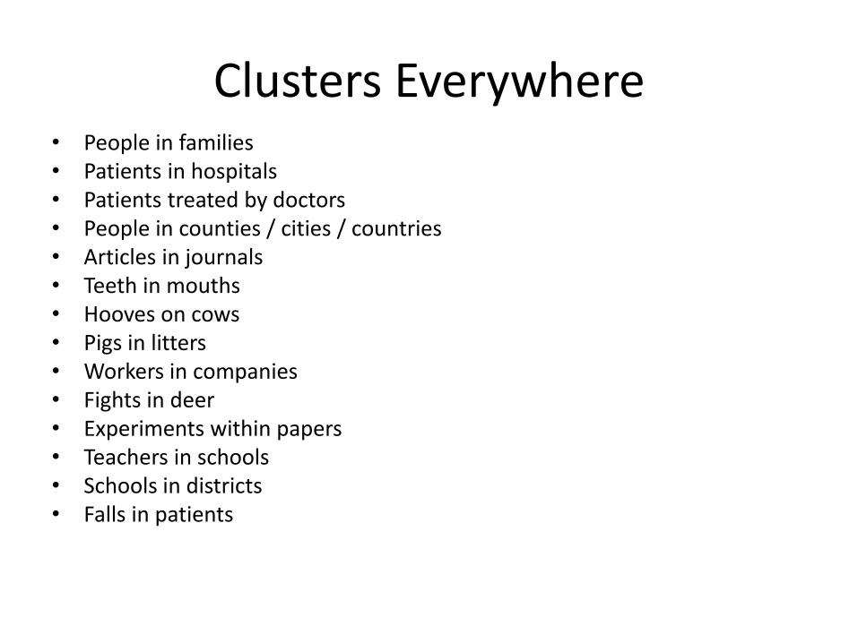
Clusters Everywhere • People in families • Patients in hospitals • Patients treated by doctors • People in counties / cities / countries • Articles in journals • Teeth in mouths • Hooves on cows • Pigs in litters • Workers in companies • Fights in deer • Experiments within papers • Teachers in schools • Schools in districts • Falls in patients

Conclusion
• Clustered data are common
• Clustered data are problematic
Number of people
>
Effect Sample Size
>
Number of clusters

• Failing to take clustering into account
– Dramatic increases in Type I error rate
• Even small ICCs can increase Type I error rate from 0.05 to 0.50
– This is bad
– We need to deal with it
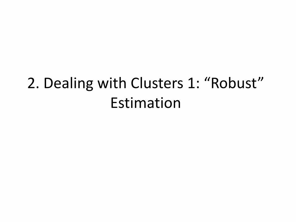
2. Dealing with Clusters 1: “Robust” Estimation
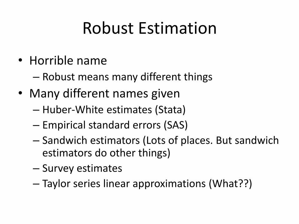
Robust Estimation
• Horrible name – Robust means many different things
• Many different names given – Huber-White estimates (Stata)
– Empirical standard errors (SAS)
– Sandwich estimators (Lots of places. But sandwich estimators do other things)
– Survey estimates
– Taylor series linear approximations (What??)

What do they do?
• Correct for i.i.d. assumption
– Independent and identically distributed
• Correct standard errors for clustering
• Correct for heteroscedasticity
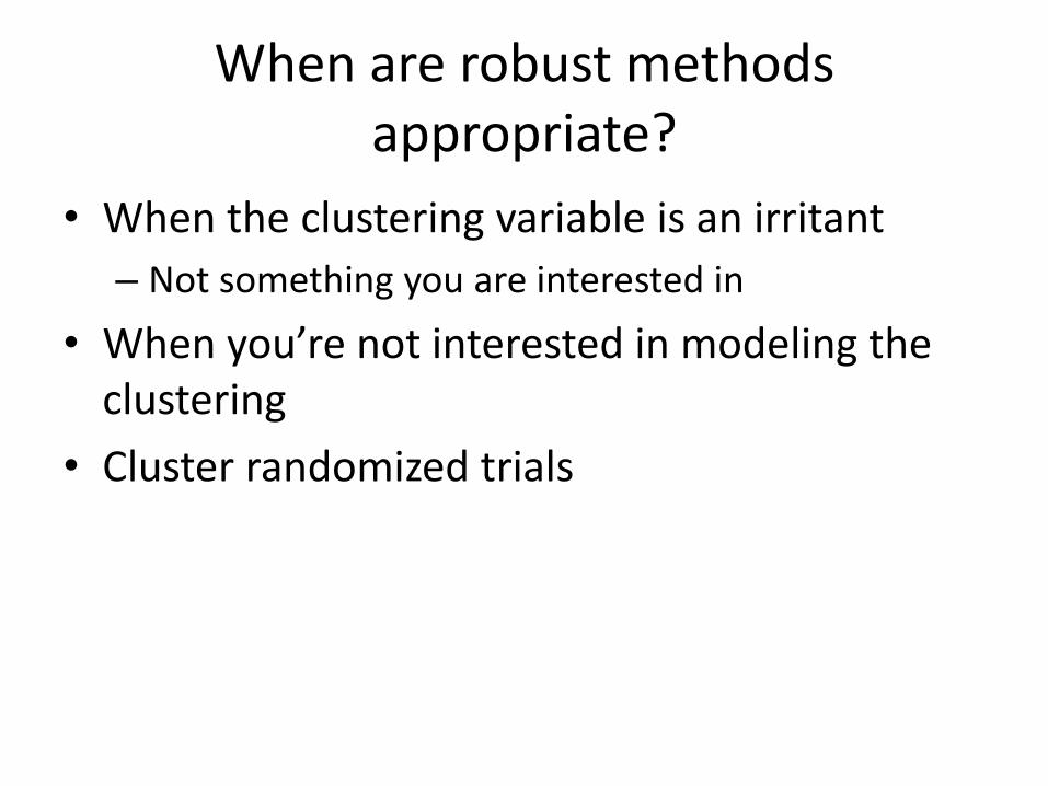
When are robust methods appropriate?
• When the clustering variable is an irritant
– Not something you are interested in
• When you’re not interested in modeling the clustering
• Cluster randomized trials
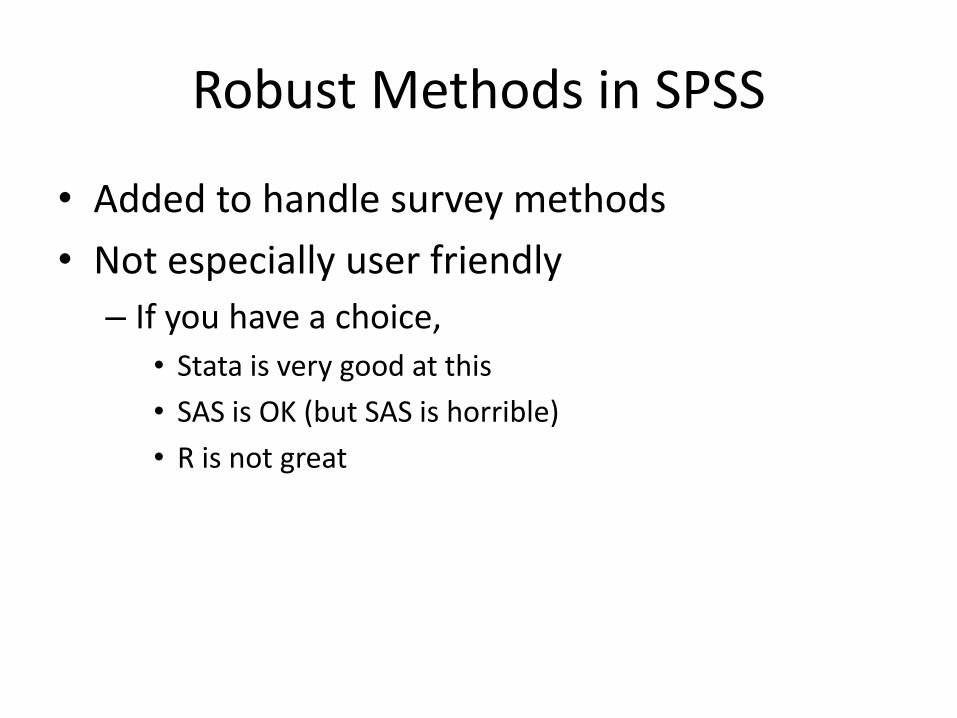
Robust Methods in SPSS
• Added to handle survey methods
• Not especially user friendly
– If you have a choice,
• Stata is very good at this
• SAS is OK (but SAS is horrible)
• R is not great
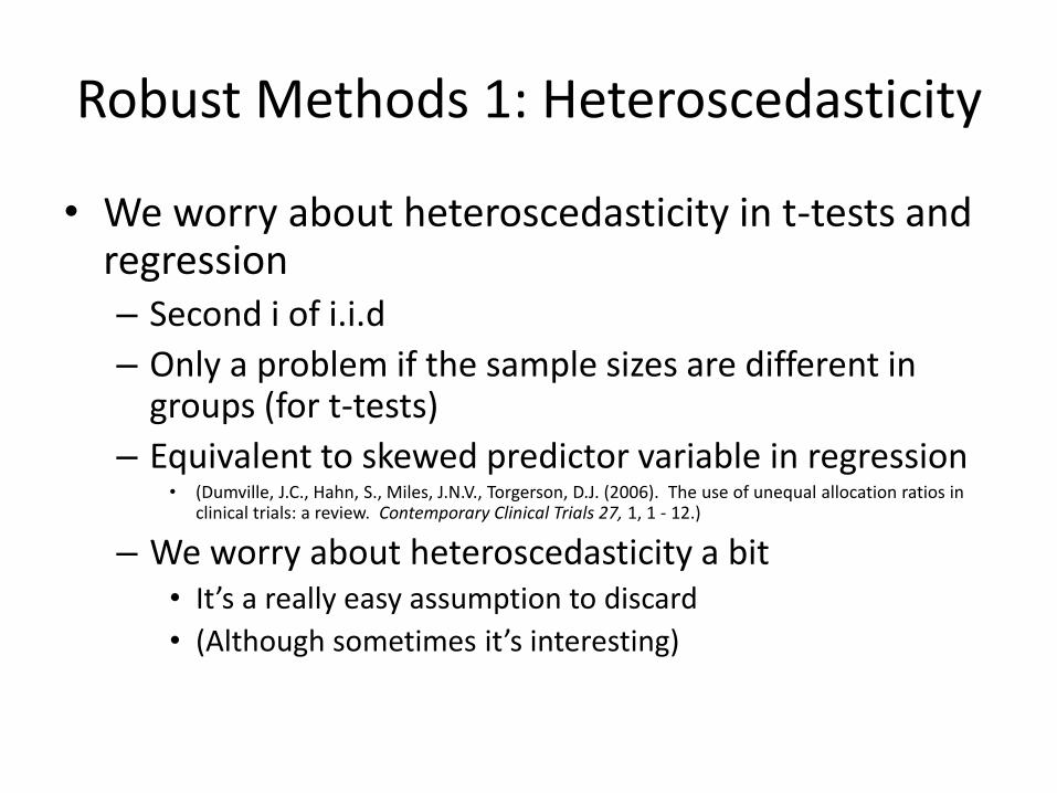
Robust Methods 1: Heteroscedasticity
• We worry about heteroscedasticity in t-tests and regression – Second i of i.i.d
– Only a problem if the sample sizes are different in groups (for t-tests)
– Equivalent to skewed predictor variable in regression • (Dumville, J.C., Hahn, S., Miles, J.N.V., Torgerson, D.J. (2006). The use of unequal allocation ratios in
clinical trials: a review. Contemporary Clinical Trials 27, 1, 1 - 12.)
– We worry about heteroscedasticity a bit • It’s a really easy assumption to discard
• (Although sometimes it’s interesting)
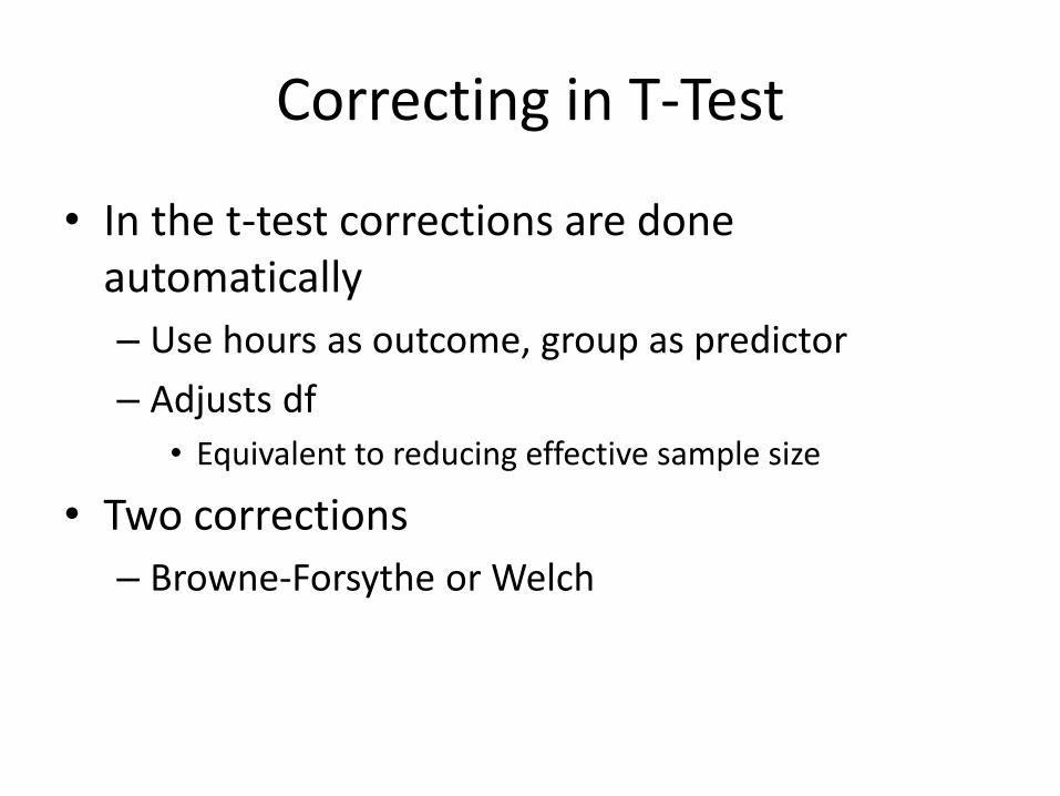
Correcting in T-Test
• In the t-test corrections are done automatically
– Use hours as outcome, group as predictor
– Adjusts df
• Equivalent to reducing effective sample size
• Two corrections
– Browne-Forsythe or Welch

Results
• Differences are small (here)
– Uncorrected: p = 0.148
– Corrected: p = 0.150
• That’s a t-test
– How do we do it for regression?
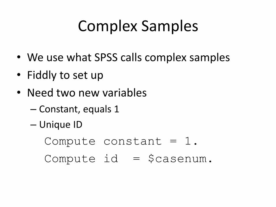
Complex Samples
• We use what SPSS calls complex samples
• Fiddly to set up
• Need two new variables
– Constant, equals 1
– Unique ID
Compute constant = 1.
Compute id = $casenum.
Complex Samples
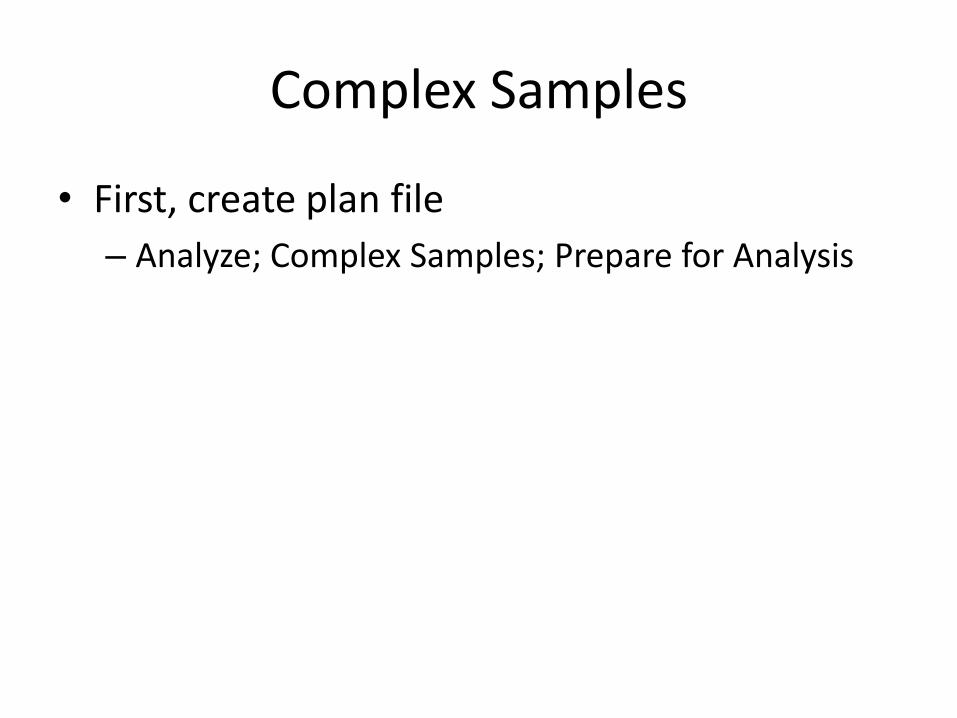
• First, create plan file
– Analyze; Complex Samples; Prepare for Analysis

We’re creating a file

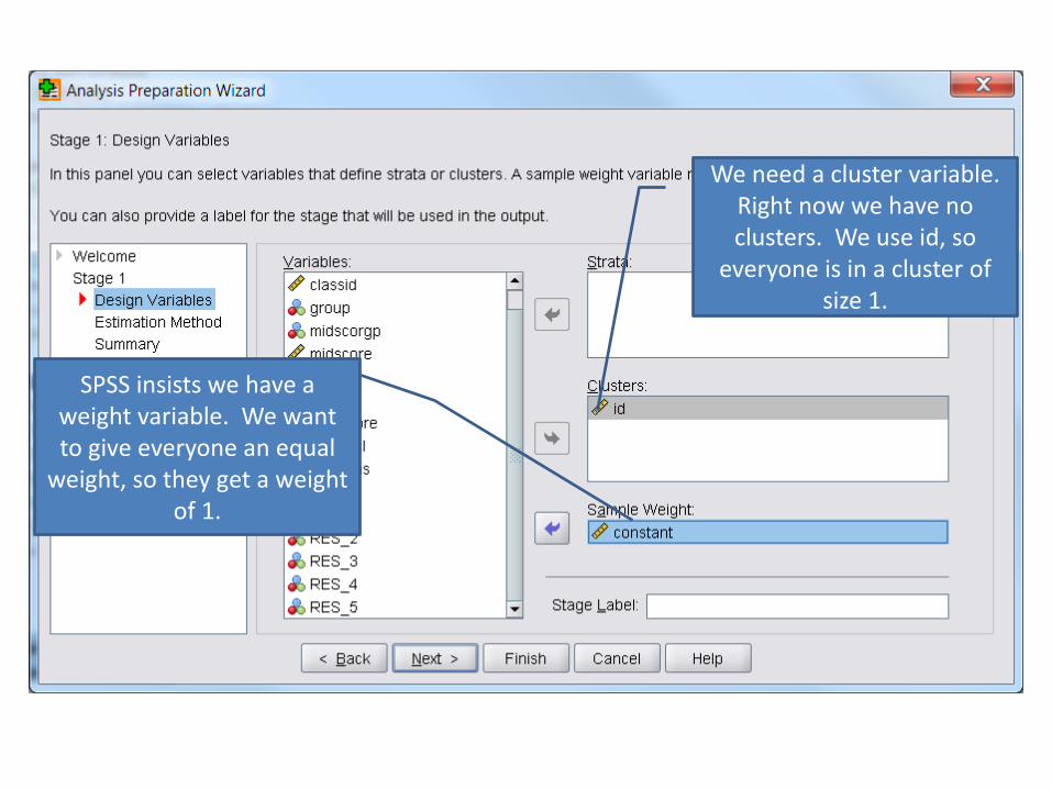
We need a cluster variable. Right now we have no clusters. We use id, so
everyone is in a cluster of size 1.
SPSS insists we have a weight variable. We want to give everyone an equal
weight, so they get a weight of 1.

Leave this alone.
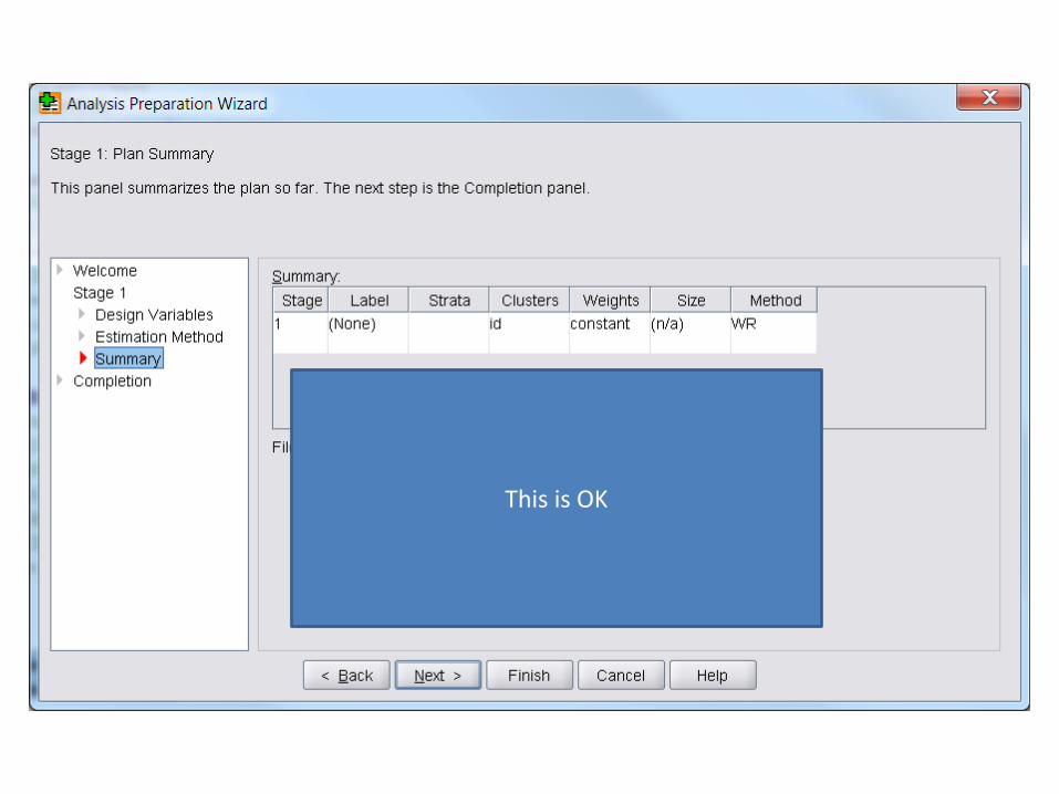
This is OK
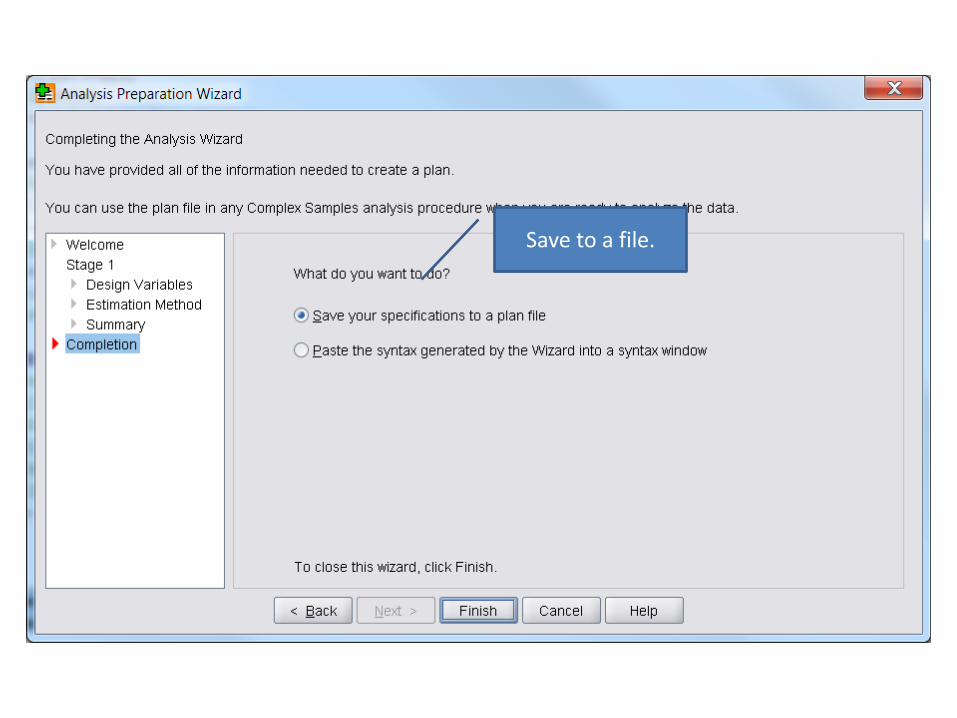
Save to a file.
Running Complex Samples
• Analyze; Complex Samples; General Linear Model
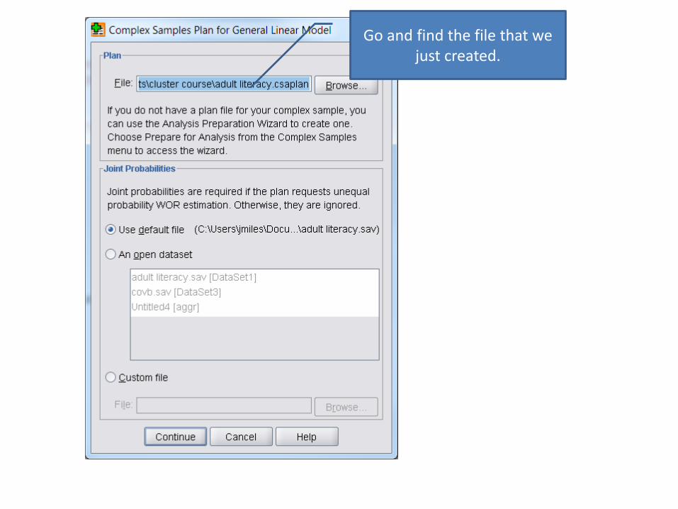
Go and find the file that we just created.

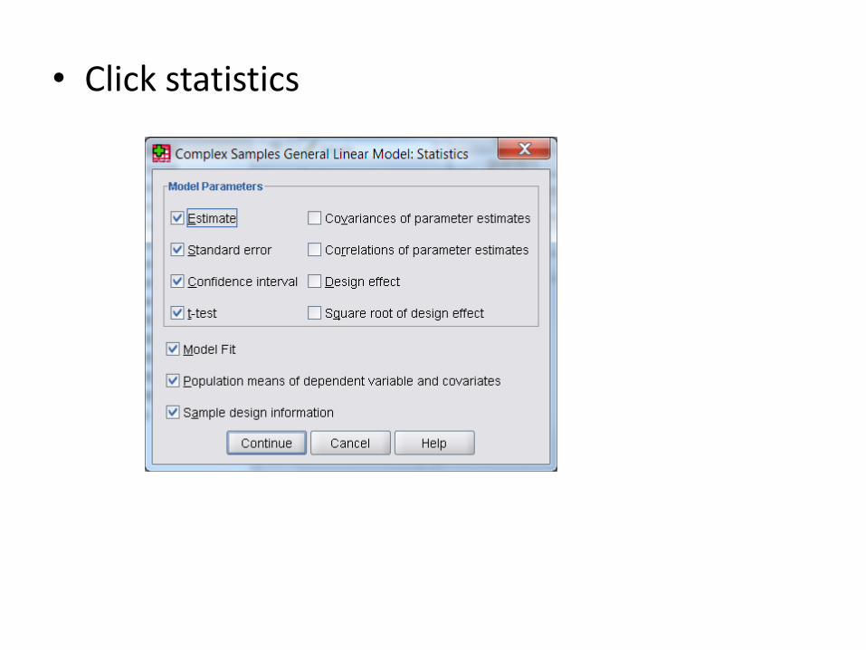
• Click statistics
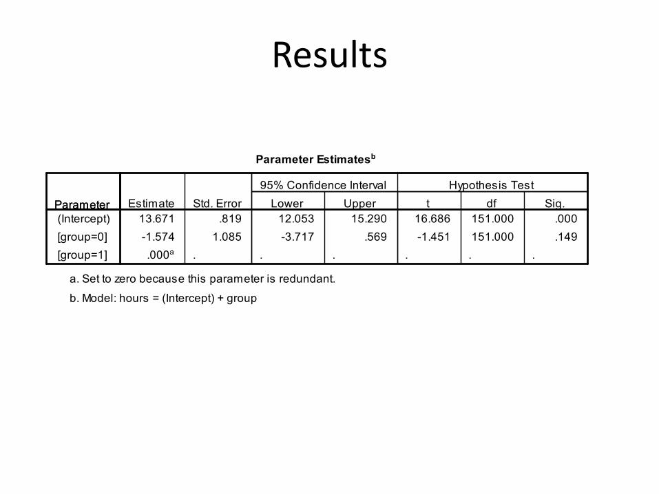
Results
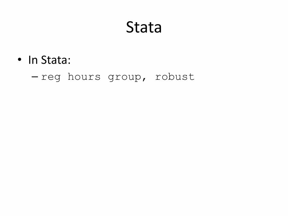
Stata
• In Stata: – reg hours group, robust

Predicting Salary
• Use employee data.sav • Set up complex sample as before
– Need constant and ID – General Linear Model – Predict Salary with
• Gender • Jobcat • Minority • Education • Salbegin • Jobtime • Prevexp

Change to Main Effects and then push all variables across
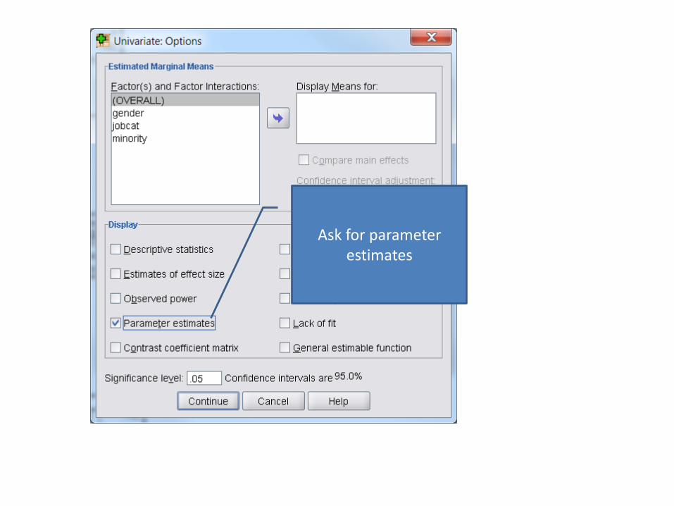
Ask for parameter estimates

A Robust Haiku
T-stat looks too good.
Use robust standard errors.
Significance gone.
Back to Clustering
• We can correct for clusters using complex samples
• Instead of ID in the cluster variable
– Class_id into the cluster variable
• What do you find?
People as Clusters
• People can be clusters
• Use co2.sav • (Wetherell, M.A., Crown, A.L., Lightman, S.L., Miles, J.N.V., Kaye, J. and
Vedhara, K. (2006). The 4-dimensional Stress Test: Psychological, Sympathetic-Adrenal-Medullary, Parasympathetic and Hypothalamic-Pituitary-Adrenal Responses Following Inhalation of 35% CO2. Psychoneuroendicronology, 31, 6, 736-747.)
• Several measures before, during and after a stress test.
– Heart rate
– Blood pressure
Repeated Measures T-Test
• (Use CO2 – HR-10.0.sav)
• Two measures of heart rate
– 10 mins before task
– During

Adding Clusters