Metrological set-up for calibrating two dimensional grid

MacroScale Recent developments in traceable dimensional measurements

1 This work is licensed under the Creative Commons Attribution 4.0 International License. To view a copy of this license, visit http://creativecommons.org/licenses/by/4.0/.

Metrological set-up for calibrating two dimensional grid plates with sub-micrometre precision

Rok Klobucar 1,*, Michael McCarthy2 and Bojan Acko 1

1 University of Maribor, Faculty of Mechanical Engineering, Maribor, Smetanova 17, Slovenia 2 University College London, Faculty of Engineering Science, London, WC1E 6BT. UK

* [email protected]

Abstract

Calibration, verification and error correction of 2D optical instruments, such as profile projectors, microscopes and “vision” systems are mainly based on measuring 2D reference grid plates. A high resolution 2D measurement instrument developed for calibrating precision grid-plates up to 300 mm x 200 mm in size with sub-micrometre measurement uncertainty is presented in this paper.

The aim of the development presented here was not to establish the highest metrological level in this field, but more importantly to align with customers’ needs, budgets and expectations within Slovenia and some neighbouring countries. Customers such as calibration laboratories and industrial companies require affordable calibrations with acceptable precision.

1 Introduction Many industrial dimensional measurement tasks require application of precise optical 2D measurement instruments, such as optical profile projectors, microscopes and “vision” systems [1]. Typical accuracies of such commercially available instruments are in the range of few micrometres. In order to assure traceability of measurements to the SI, these instruments are normally calibrated by using different line standards such as precision line scales, stage micrometres, linewidth standards, grid plates, and standards with different special patterns [2,3]. With these standards, different kind of vision system, artefacts and algorithms for image processing could be verified and evaluated [4,5].

Larger corporate companies, may have their own internal accredited calibration facilities, while for smaller companies calibrations are typically provided by external providers such as accredited calibration laboratories. These accredited laboratories assure traceability of their line standards to a national metrological institute. Growing demands on the precision of such calibrations require new and better instrumentation, as well as new calibration methods and improved precision. While very high accuracy level for the calibration of line scales is widely achievable [6-11], only a very few laboratories in the world are able to calibrate grid plates with sufficient precision [12-19]. A preliminary survey on the calibration services from various national metrology institutes (NMLs) shows that 37 institutes around the World (20 of these in Europe) offer calibration of line scales, while only 6 institutes in the World (3 in Europe) can calibrate grid plates [20]. Only one European national metrology institute offers calibration services for grid plates of dimension 200 mm x 300 mm, which are normally delivered using modern digital (“vision”) 2D optical measurement instruments.

Accredited laboratories offering grid plate calibration services at sufficient levels of precision, are also very rare and difficult to find and thus support for the performance verification of 2D optical instruments can be weak. This is particularly true in the case of Slovenia and to that end during the past few years our national metrology laboratory for length put a lot of effort into initially developing instrumentation and procedures for calibrating line standards. A few years ago this was realised and we were accredited to provide calibrations for line scales up to 500 mm [21]. The Laboratory for Production Measurement (MIRS/UM-FS/LTM) is a EURAMET designated institute (MIRS/UM-FS/LTM) was the pilot laboratory in the CCL-K7 inter-laboratory comparison on line scales [11]. Following this we have now been intensively exploring the possibility for developing the capability further in order to calibrate grid plates with an area up to dimensions 200 mm x 300 mm. This decision was based on a series of requests

DOI: 10.7795/810.20180323E

mailto:rok.klobucar@



from both our accredited calibration laboratories and industrial companies. Many advanced technologies employ measurement systems [22] that require precise calibration of optical measurement components. The research presented here has resulted in a new measurement set-up of our line scale facility combined with supporting procedures. An application for an extension to our accreditation has already been sent to our Slovenian national accreditation body. Our research work has been supported by University College London, Faculty of Engineering Science.

2 Measurement set-up

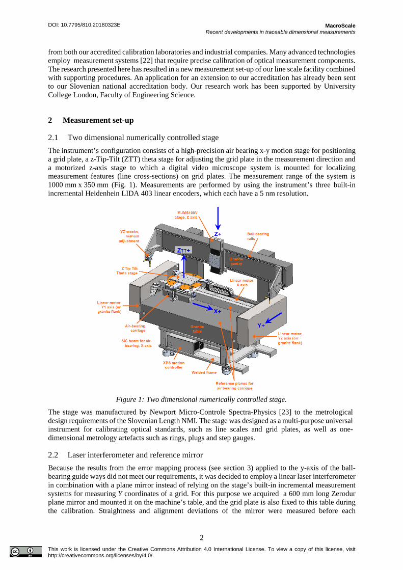
2.1 Two dimensional numerically controlled stage The instrument’s configuration consists of a high-precision air bearing x-y motion stage for positioning a grid plate, a z-Tip-Tilt (ZTT) theta stage for adjusting the grid plate in the measurement direction and a motorized z-axis stage to which a digital video microscope system is mounted for localizing measurement features (line cross-sections) on grid plates. The measurement range of the system is 1000 mm x 350 mm (Fig. 1). Measurements are performed by using the instrument’s three built-in incremental Heidenhein LIDA 403 linear encoders, which each have a 5 nm resolution.

Figure 1: Two dimensional numerically controlled stage.

The stage was manufactured by Newport Micro-Controle Spectra-Physics [23] to the metrological design requirements of the Slovenian Length NMI. The stage was designed as a multi-purpose universal instrument for calibrating optical standards, such as line scales and grid plates, as well as one-dimensional metrology artefacts such as rings, plugs and step gauges.

2.2 Laser interferometer and reference mirror Because the results from the error mapping process (see section 3) applied to the y-axis of the ball-bearing guide ways did not meet our requirements, it was decided to employ a linear laser interferometer in combination with a plane mirror instead of relying on the stage’s built-in incremental measurement systems for measuring Y coordinates of a grid. For this purpose we acquired a 600 mm long Zerodur plane mirror and mounted it on the machine’s table, and the grid plate is also fixed to this table during the calibration. Straightness and alignment deviations of the mirror were measured before each

DOI: 10.7795/810.20180323E



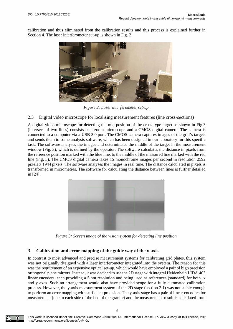
calibration and thus eliminated from the calibration results and this process is explained further in Section 4. The laser interferometer set-up is shown in Fig. 2.

Figure 2: Laser interferometer set-up.

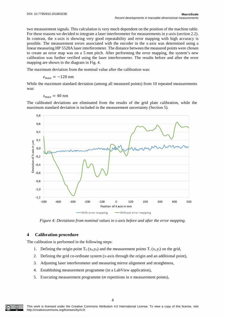
2.3 Digital video microscope for localising measurement features (line cross-sections) A digital video microscope for detecting the mid-position of the cross type target as shown in Fig 3 (intersect of two lines) consists of a zoom microscope and a CMOS digital camera. The camera is connected to a computer via a USB 3.0 port. The CMOS camera captures images of the grid’s targets and sends them to some analysis software, which has been designed in our laboratory for this specific task. The software analyses the images and determinates the middle of the target in the measurement window (Fig. 3), which is defined by the operator. The software calculates the distance in pixels from the reference position marked with the blue line, to the middle of the measured line marked with the red line (Fig. 3). The CMOS digital camera takes 15 monochrome images per second in resolution 2592 pixels x 1944 pixels. The software analyses the images in real time. The distance calculated in pixels is transformed in micrometres. The software for calculating the distance between lines is further detailed in [24].

Figure 3: Screen image of the vision system for detecting line position.

3 Calibration and error mapping of the guide way of the x-axis In contrast to most advanced and precise measurement systems for calibrating grid plates, this system was not originally designed with a laser interferometer integrated into the system. The reason for this was the requirement of an expensive optical set-up, which would have employed a pair of high precision orthogonal plane mirrors. Instead, it was decided to use the 2D stage with integral Heidenhein LIDA 403 linear encoders, each providing a 5 nm resolution and being used as references (standard) for both x and y axes. Such an arrangement would also have provided scope for a fully automated calibration process. However, the y-axis measurement system of the 2D stage (section 2.1) was not stable enough to perform an error mapping with sufficient precision. The y-axis stage has a pair of linear encoders for measurement (one to each side of the bed of the granite) and the measurement result is calculated from

DOI: 10.7795/810.20180323E



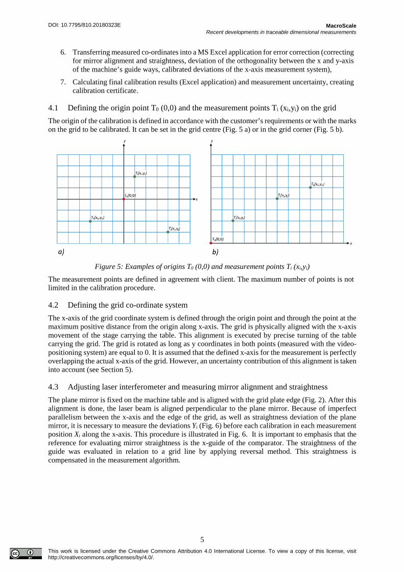
two measurement signals. This calculation is very much dependent on the position of the machine table. For these reasons we decided to integrate a laser interferometer for measurements in y-axis (section 2.2). In contrast, the x-axis is showing very good repeatability and error mapping with high accuracy is possible. The measurement errors associated with the encoder in the x-axis was determined using a linear measuring HP 5528A laser interferometer. The distance between the measured points were chosen to create an error map was on a 5 mm pitch. After performing the error mapping, the system’s new calibration was further verified using the laser interferometer. The results before and after the error mapping are shown in the diagram in Fig. 4.

The maximum deviation from the nominal value after the calibration was:

𝑒𝑒𝑚𝑚𝑚𝑚𝑚𝑚 = −120 nm

While the maximum standard deviation (among all measured points) from 10 repeated measurements was:

𝑠𝑠𝑚𝑚𝑚𝑚𝑚𝑚 = 40 nm

The calibrated deviations are eliminated from the results of the grid plate calibration, while the maximum standard deviation is included in the measurement uncertainty (Section 5).

Figure 4: Deviations from nominal values in x-axis before and after the error mapping.

4 Calibration procedure The calibration is performed in the following steps:

1. Defining the origin point T0 (x0,y0) and the measurement points Ti (xi,yi) on the grid,

2. Defining the grid co-ordinate system (x-axis through the origin and an additional point),

3. Adjusting laser interferometer and measuring mirror alignment and straightness,

4. Establishing measurement programme (in a LabView application),

5. Executing measurement programme (m repetitions in n measurement points),

DOI: 10.7795/810.20180323E



6. Transferring measured co-ordinates into a MS Excel application for error correction (correcting for mirror alignment and straightness, deviation of the orthogonality between the x and y-axis of the machine’s guide ways, calibrated deviations of the x-axis measurement system),

7. Calculating final calibration results (Excel application) and measurement uncertainty, creating calibration certificate.

4.1 Defining the origin point T0 (0,0) and the measurement points Ti (xi,yi) on the grid The origin of the calibration is defined in accordance with the customer’s requirements or with the marks on the grid to be calibrated. It can be set in the grid centre (Fig. 5 a) or in the grid corner (Fig. 5 b).

Figure 5: Examples of origins T0 (0,0) and measurement points Ti (xi,yi)

The measurement points are defined in agreement with client. The maximum number of points is not limited in the calibration procedure.

4.2 Defining the grid co-ordinate system The x-axis of the grid coordinate system is defined through the origin point and through the point at the maximum positive distance from the origin along x-axis. The grid is physically aligned with the x-axis movement of the stage carrying the table. This alignment is executed by precise turning of the table carrying the grid. The grid is rotated as long as y coordinates in both points (measured with the video-positioning system) are equal to 0. It is assumed that the defined x-axis for the measurement is perfectly overlapping the actual x-axis of the grid. However, an uncertainty contribution of this alignment is taken into account (see Section 5).

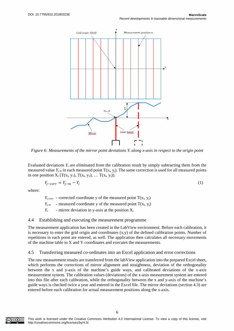
4.3 Adjusting laser interferometer and measuring mirror alignment and straightness The plane mirror is fixed on the machine table and is aligned with the grid plate edge (Fig. 2). After this alignment is done, the laser beam is aligned perpendicular to the plane mirror. Because of imperfect parallelism between the x-axis and the edge of the grid, as well as straightness deviation of the plane mirror, it is necessary to measure the deviations Yi (Fig. 6) before each calibration in each measurement position Xi along the x-axis. This procedure is illustrated in Fig. 6. It is important to emphasis that the reference for evaluating mirror straightness is the x-guide of the comparator. The straightness of the guide was evaluated in relation to a grid line by applying reversal method. This straightness is compensated in the measurement algorithm.

DOI: 10.7795/810.20180323E



Figure 6: Measurements of the mirror point deviations Yi along x-axis in respect to the origin point

Evaluated deviations Yi are eliminated from the calibration result by simply subtracting them from the measured value Yj-m in each measured point T(xi, yj). The same correction is used for all measured points in one position Xi (T(xi, y1), T(xi, y2), … T(xi, yj)).

𝑌𝑌𝑗𝑗−𝑐𝑐𝑐𝑐𝑐𝑐𝑐𝑐 = 𝑌𝑌𝑗𝑗−𝑚𝑚 − 𝑌𝑌𝑖𝑖 (1)

where:

Yj-corr - corrected coordinate y of the measured point T(xi, yj) Yj-m - measured coordinate y of the measured point T(xi, yj) Yi - mirror deviation in y-axis at the position Xi

4.4 Establishing and executing the measurement programme The measurement application has been created in the LabView environment. Before each calibration, it is necessary to enter the grid origin and coordinates (x,y) of the defined calibration points. Number of repetitions in each point are entered, as well. The application then calculates all necessary movements of the machine table in X and Y coordinates and executes the measurements.

4.5 Transferring measured co-ordinates into an Excel application and error corrections The raw measurement results are transferred from the labView application into the prepared Excel sheet, which performs the corrections of mirror alignment and straightness, deviation of the orthogonality between the x and y-axis of the machine’s guide ways, and calibrated deviations of the x-axis measurement system. The calibration values (deviations) of the x-axis measurement system are entered into this file after each calibration, while the orthogonality between the x and y-axis of the machine’s guide ways is checked twice a year and entered in the Excel file. The mirror deviations (section 4.3) are entered before each calibration for actual measurement positions along the x-axis.

DOI: 10.7795/810.20180323E



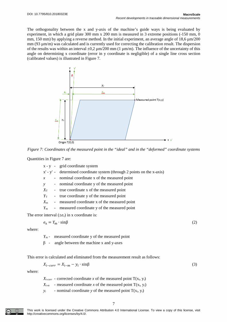
The orthogonality between the x and y-axis of the machine’s guide ways is being evaluated by experiment, in which a grid plate 300 mm x 200 mm is measured in 3 extreme positions (-150 mm, 0 mm, 150 mm) by applying a reverse method. In the initial experiment, an average angle of 18,6 µm/200 mm (93 µm/m) was calculated and is currently used for correcting the calibration result. The dispersion of the results was within an interval ±0,2 µm/200 mm (1 µm/m). The influence of the uncertainty of this angle on determining x coordinate (error in y coordinate is negligible) of a single line cross section (calibrated values) is illustrated in Figure 7.

Figure 7: Coordinates of the measured point in the “ideal” and in the “deformed” coordinate systems

Quantities in Figure 7 are:

x - y - grid coordinate system x' - y' - determined coordinate system (through 2 points on the x-axis) x - nominal coordinate x of the measured point y - nominal coordinate y of the measured point XT - true coordinate x of the measured point YT - true coordinate y of the measured point Xm - measured coordinate x of the measured point Ym - measured coordinate y of the measured point

The error interval (±ex) in x coordinate is:

𝑒𝑒x = 𝑌𝑌m ∙ sinβ (2)

where:

Ym - measured coordinate y of the measured point β - angle between the machine x and y-axes

This error is calculated and eliminated from the measurement result as follows:

𝑋𝑋𝑖𝑖−𝑐𝑐𝑐𝑐𝑐𝑐𝑐𝑐 = 𝑋𝑋i−m − 𝑦𝑦𝑖𝑖 ∙ sinβ (3)

where:

Xi-corr - corrected coordinate x of the measured point T(xi, yi) Xi-m - measured coordinate x of the measured point T(xi, yi) yi - nominal coordinate y of the measured point T(xi, yi)

DOI: 10.7795/810.20180323E



5 Measurement uncertainty The mathematical model of measurement for both axes is defined by equations (4) and (5).

a) For x-axis (measured with the machine measurement system):

𝑋𝑋𝑐𝑐 = 𝑋𝑋𝑖𝑖 − 𝑒𝑒𝑚𝑚𝑚𝑚 − 𝑒𝑒𝑝𝑝𝑚𝑚 − 𝑒𝑒𝑠𝑠𝑚𝑚 + 𝑋𝑋 ∙ (𝛼𝛼� ∙ ∆𝑇𝑇 − �̅�𝜃 ∙ �̅�𝜃) + 𝑒𝑒𝐿𝐿𝐿𝐿 (4)

b) For y-axis (measured with the laser interferometer and plane mirror):

𝑌𝑌𝑐𝑐 = 𝑌𝑌𝑖𝑖 − 𝑒𝑒𝑑𝑑𝑝𝑝 − 𝑒𝑒𝑐𝑐𝑐𝑐𝑠𝑠 − 𝑒𝑒𝑚𝑚𝑎𝑎 − 𝑒𝑒𝑝𝑝𝑎𝑎 − 𝑒𝑒𝑠𝑠𝑎𝑎 − 𝑒𝑒𝑚𝑚𝑠𝑠 − 𝑌𝑌 ∙ 𝛼𝛼𝐺𝐺 ∙ 𝜃𝜃𝐺𝐺 + 𝑒𝑒𝐿𝐿𝐿𝐿 (5)

where:

𝑋𝑋𝑐𝑐 - calibrated (reported) value of x coordinate 𝑋𝑋𝑖𝑖 - measurement standard (Newport 2D) indication of x coordinate 𝑋𝑋 - nominal x-coordinate of the measured point 𝑒𝑒𝑚𝑚𝑚𝑚 - error in x-axis due to the alignment of the grid coordinate system 𝑒𝑒𝑝𝑝𝑚𝑚 - error in x-axis due to the orthogonality deviation of the measurement system axes x

and y 𝑒𝑒𝑠𝑠𝑚𝑚 - error in x-axis due to the straightness deviation of the comparator y-axis 𝛼𝛼� - average linear temperature expansion coefficient of the machine (Newport 2D)

measurement system (x-axis) and the grid plate ∆𝑇𝑇 - difference between the machine measurement system temperature and the grid plate

temperature �̅�𝜃 - average temperature deviation from 20 °C of the machine measurement system and

the grid plate ∆𝛼𝛼 - difference between the temperature expansion coefficients of the machine

measurement system and the grid plate 𝑒𝑒𝐿𝐿𝐿𝐿 - error of the determined distance between the reference position and the measurement

position in the video probing system (assumed to be 0) 𝑌𝑌𝑐𝑐 - calibrated (reported) value of y-coordinate 𝑌𝑌𝑖𝑖 - measurement standard (LI) indication of y-coordinate 𝑌𝑌 - nominal y coordinate of the measured point 𝑒𝑒𝑑𝑑𝑝𝑝 - dead path error (assumed to be 0) 𝑒𝑒𝑐𝑐𝑐𝑐𝑠𝑠 - cosine error (alignment of LI; assumed to be 0) 𝑒𝑒𝑚𝑚𝑎𝑎 - error in y-axis due to the alignment of the grid coordinate system 𝑒𝑒𝑝𝑝𝑎𝑎 - error in y-axis due to the orthogonality deviation of the measurement system x and y-

axes 𝑒𝑒𝑠𝑠𝑎𝑎 - error in y-axis due to the straightness deviation of the comparator x-axis 𝑒𝑒𝑚𝑚𝑠𝑠 - error in y-axis due to the mirror straightness and adjustment deviations in the

measurement position along x-axis 𝛼𝛼𝐺𝐺 - linear temperature expansion coefficient of the calibrated grid plate 𝜃𝜃𝐺𝐺 - temperature deviation of the calibrated grid plate from 20 °C

For the CMC evaluation, a grid plate will be one which has been manufactured very close to its nominal design and furthermore, the quality of the lines structures and their line edges are of high quality. Standard uncertainties of all influence values [25-27], as well as the sensitivity coefficients and final contributions are presented in the uncertainty budget in Table 1 and Table 2. Specific description will only be given for 3 influence values:

DOI: 10.7795/810.20180323E



• Uncertainty of determining the distance between the reference position and the measurement position in the video probing system u(eLV)

• Uncertainty due to the orthogonality deviation of the measurement system axes x and y u(epx) and

• Uncertainty due to the alignment of the grid coordinate system u(eax).

These quantities represent the focus of the presented research.

5.1 Uncertainty of determining the distance between the reference position and the measurement position in the video probing system u(eLV)

The distance between the measurement and the reference position Lv (blue and red line in Fig. 3) is defined by the following mathematical model:

Lv = Lref * P/Pref = R*P (6)

where:

Lv - distance between the measurement and reference position Lref - length of the scale mark movement at resolution determination P - number of pixels at measurement (distance between the measurement and reference

line) Pref - number of pixels at resolution determination (distance between the start and end

position of the reference line) R - pixel size

The combined uncertainty is:

uc2(Lv) = cR

2u2(R)+c P2u2(P) (7)

where ci are partial derivatives of the function (6):

cR = ∂f/∂R = P; Pmax = 100 cP = ∂f/∂P = R = 0,018 µm

Pixel size R was determined by repeating measurements and amounts to R = 0,000090 mm for applied optical enlargement (50X), at the uncertainty of the pixel size of u(R) = 0,001 µm.

Number of pixels between the reference and measurement position P is rounded up to integer. Standard uncertainty of determining the number of pixels at presumed rectangular distribution is:

29,03/5,03/)( === IPu

Uncertainty of the distance between the measurement and reference position in the video window u(eLV) is then:

u(eLv) = 130 nm

5.2 Uncertainty due to the orthogonality deviation of the measurement system axes x and y u(epx)

Geometrical relations and the results of performed experiment are explained in Section 4.5 (Fig. 7). Error in y-axis is negligible, while the error in x-axis is calculated and eliminated from the measurement result (equations (2) and (3)). However, possible error interval of the angle β calculation (experiment – span of calculated β in different table positions) is evaluated to be:

𝑒𝑒α = 1 µm/m

The error interval ex is then:

𝑒𝑒px = ±10−6 ∙ 𝑌𝑌m ≈ ±10−6 ∙ 𝑦𝑦

DOI: 10.7795/810.20180323E



Standard uncertainty at presumed rectangular distribution is:

𝑢𝑢(𝑒𝑒px) = 10−6 ∙ 𝑦𝑦 /√3 ≈ 5,8 ∙ 10−7 ∙ 𝑦𝑦

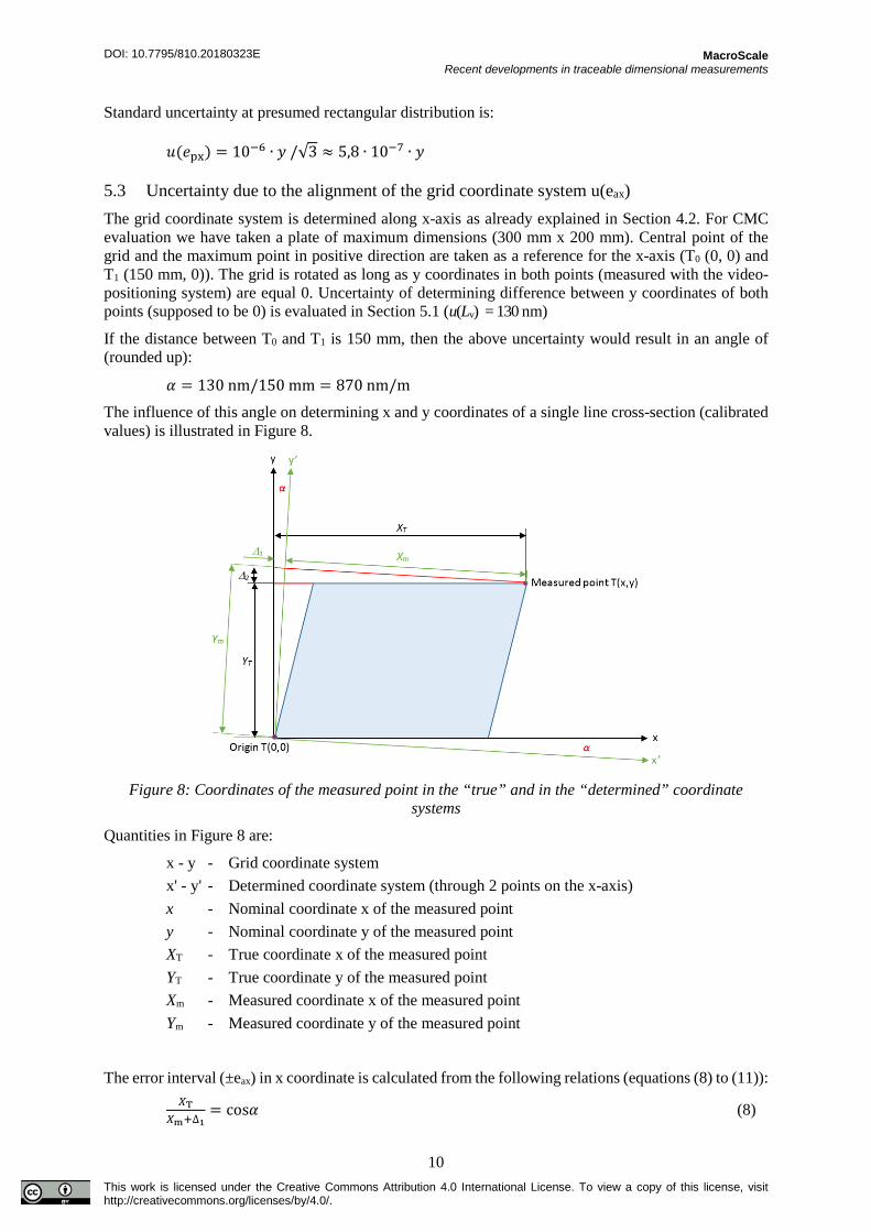
5.3 Uncertainty due to the alignment of the grid coordinate system u(eax) The grid coordinate system is determined along x-axis as already explained in Section 4.2. For CMC evaluation we have taken a plate of maximum dimensions (300 mm x 200 mm). Central point of the grid and the maximum point in positive direction are taken as a reference for the x-axis (T0 (0, 0) and T1 (150 mm, 0)). The grid is rotated as long as y coordinates in both points (measured with the video-positioning system) are equal 0. Uncertainty of determining difference between y coordinates of both points (supposed to be 0) is evaluated in Section 5.1 (u(Lv) = 130 nm)

If the distance between T0 and T1 is 150 mm, then the above uncertainty would result in an angle of (rounded up):

𝛼𝛼 = 130 nm/150 mm = 870 nm/m The influence of this angle on determining x and y coordinates of a single line cross-section (calibrated values) is illustrated in Figure 8.

Figure 8: Coordinates of the measured point in the “true” and in the “determined” coordinate

systems

Quantities in Figure 8 are:

x - y - Grid coordinate system x' - y' - Determined coordinate system (through 2 points on the x-axis) x - Nominal coordinate x of the measured point y - Nominal coordinate y of the measured point XT - True coordinate x of the measured point YT - True coordinate y of the measured point Xm - Measured coordinate x of the measured point Ym - Measured coordinate y of the measured point

The error interval (±eax) in x coordinate is calculated from the following relations (equations (8) to (11)): 𝑋𝑋T

𝑋𝑋m+∆1= cos𝛼𝛼 (8)

DOI: 10.7795/810.20180323E



𝑋𝑋T = (𝑋𝑋m + ∆1) ∙ cos𝛼𝛼 ; ∆1𝑌𝑌m

= tan𝛼𝛼 (9)

𝑋𝑋T = (𝑋𝑋m + 𝑌𝑌m ∙ tan𝛼𝛼) ∙ cos𝛼𝛼 (10)

𝑒𝑒ax = 𝑋𝑋m − (𝑋𝑋m + 𝑌𝑌m ∙ tan𝛼𝛼) ∙ cos𝛼𝛼 = 𝑋𝑋m ∙ (1 − cos𝛼𝛼)− 𝑌𝑌m ∙ sin𝛼𝛼 (11)

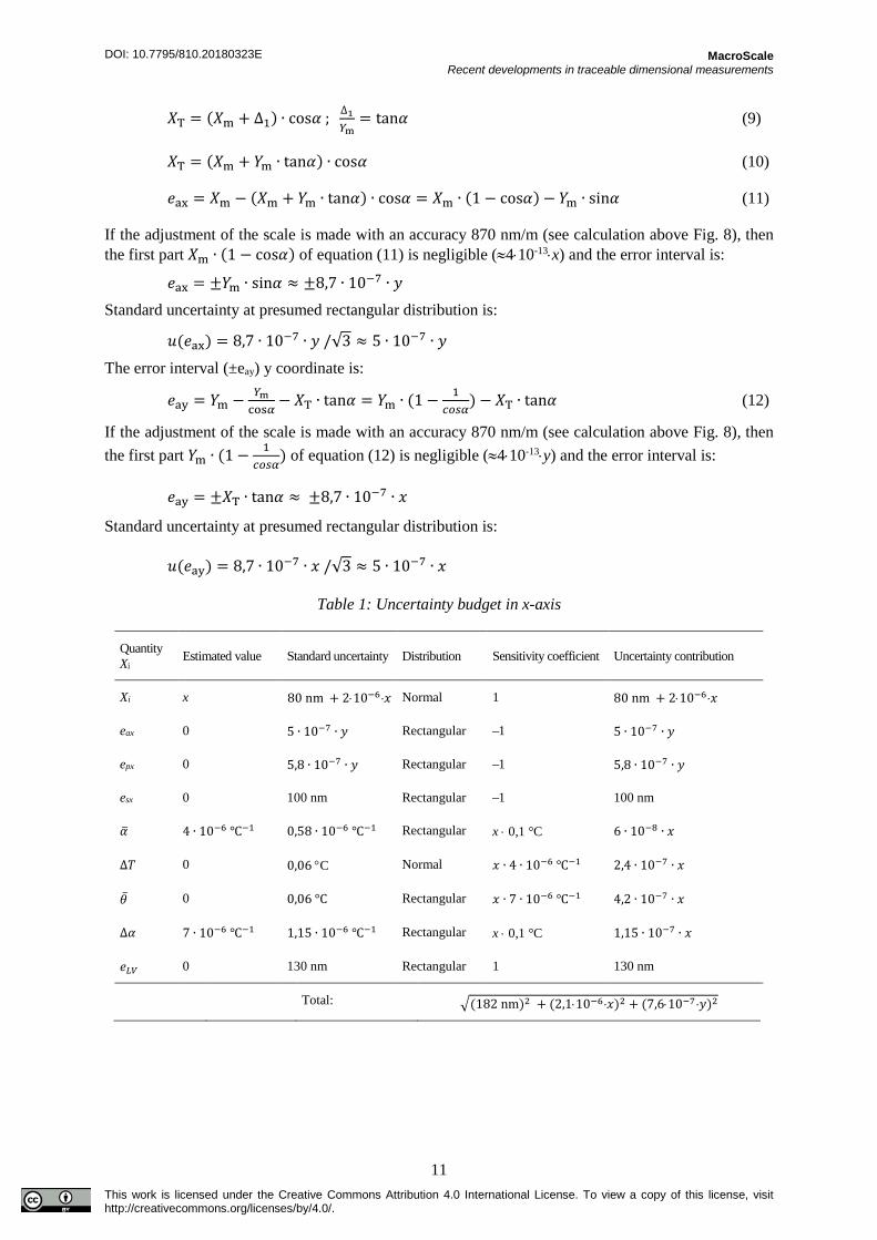
If the adjustment of the scale is made with an accuracy 870 nm/m (see calculation above Fig. 8), then the first part 𝑋𝑋m ∙ (1 − cos𝛼𝛼) of equation (11) is negligible (≈4⋅10-13⋅x) and the error interval is:

𝑒𝑒ax = ±𝑌𝑌m ∙ sin𝛼𝛼 ≈ ±8,7 ∙ 10−7 ∙ 𝑦𝑦 Standard uncertainty at presumed rectangular distribution is:

𝑢𝑢(𝑒𝑒ax) = 8,7 ∙ 10−7 ∙ 𝑦𝑦 /√3 ≈ 5 ∙ 10−7 ∙ 𝑦𝑦

The error interval (±eay) y coordinate is:

𝑒𝑒ay = 𝑌𝑌m − 𝑌𝑌mcos𝛼𝛼

− 𝑋𝑋T ∙ tan𝛼𝛼 = 𝑌𝑌m ∙ (1 − 1𝑐𝑐𝑐𝑐𝑠𝑠𝛼𝛼

) − 𝑋𝑋T ∙ tan𝛼𝛼 (12)

If the adjustment of the scale is made with an accuracy 870 nm/m (see calculation above Fig. 8), then the first part 𝑌𝑌m ∙ (1 − 1

𝑐𝑐𝑐𝑐𝑠𝑠𝛼𝛼) of equation (12) is negligible (≈4⋅10-13⋅y) and the error interval is:

𝑒𝑒ay = ±𝑋𝑋T ∙ tan𝛼𝛼 ≈ ±8,7 ∙ 10−7 ∙ 𝑥𝑥

Standard uncertainty at presumed rectangular distribution is:

𝑢𝑢(𝑒𝑒ay) = 8,7 ∙ 10−7 ∙ 𝑥𝑥 /√3 ≈ 5 ∙ 10−7 ∙ 𝑥𝑥

Table 1: Uncertainty budget in x-axis

Quantity Xi Estimated value Standard uncertainty Distribution Sensitivity coefficient Uncertainty contribution

Xi x 80 nm + 2⋅10−6⋅𝑥𝑥 Normal 1 80 nm + 2⋅10−6⋅𝑥𝑥

eax 0 5 ∙ 10−7 ∙ 𝑦𝑦 Rectangular –1 5 ∙ 10−7 ∙ 𝑦𝑦

epx 0 5,8 ∙ 10−7 ∙ 𝑦𝑦 Rectangular –1 5,8 ∙ 10−7 ∙ 𝑦𝑦

esx 0 100 nm Rectangular –1 100 nm

𝛼𝛼� 4 ∙ 10−6 ℃−1 0,58 ∙ 10−6 ℃−1 Rectangular x ⋅ 0,1 °C 6 ∙ 10−8 ∙ 𝑥𝑥

∆𝑇𝑇 0 0,06 °C Normal 𝑥𝑥 ∙ 4 ∙ 10−6 ℃−1 2,4 ∙ 10−7 ∙ 𝑥𝑥

�̅�𝜃 0 0,06 °C Rectangular 𝑥𝑥 ∙ 7 ∙ 10−6 ℃−1 4,2 ∙ 10−7 ∙ 𝑥𝑥

∆𝛼𝛼 7 ∙ 10−6 ℃−1 1,15 ∙ 10−6 ℃−1 Rectangular x ⋅ 0,1 °C 1,15 ∙ 10−7 ∙ 𝑥𝑥

𝑒𝑒𝐿𝐿𝐿𝐿 0 130 nm Rectangular 1 130 nm

Total: �(182 nm)2 + (2,1⋅10−6⋅𝑥𝑥)2 + (7,6⋅10−7⋅𝑦𝑦)2

DOI: 10.7795/810.20180323E



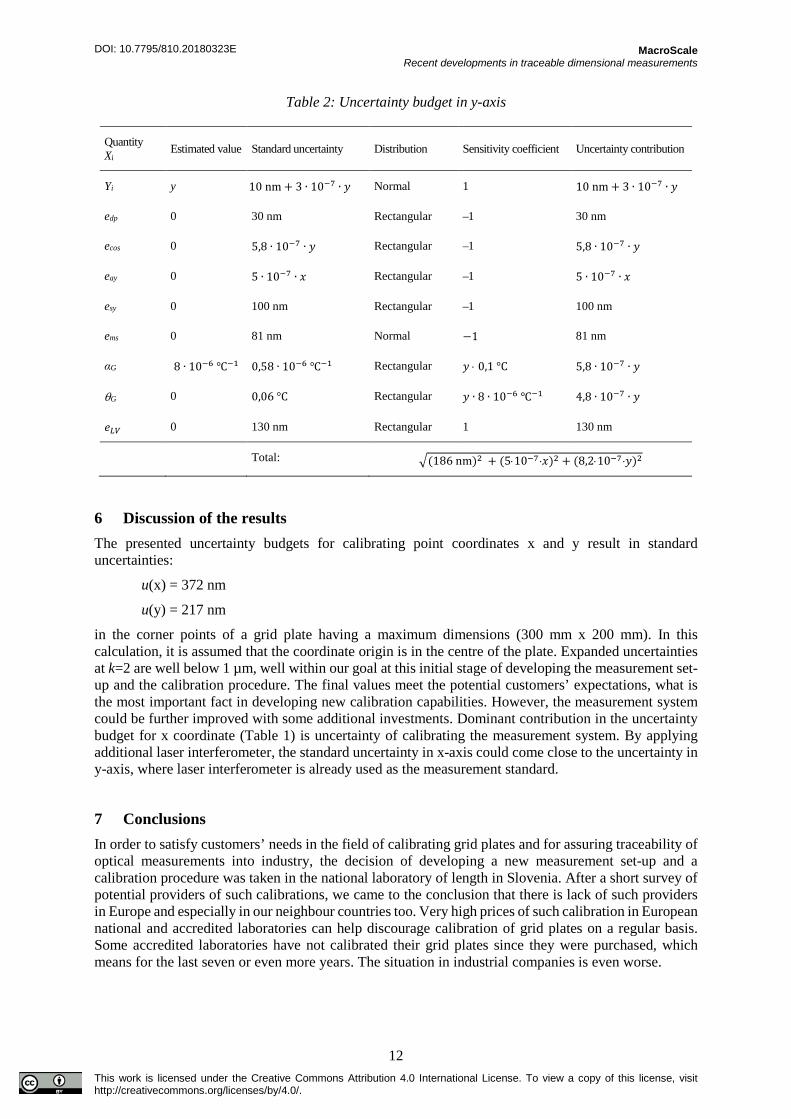
Table 2: Uncertainty budget in y-axis

Quantity Xi Estimated value Standard uncertainty Distribution Sensitivity coefficient Uncertainty contribution

Yi y 10 nm + 3 ∙ 10−7 ∙ 𝑦𝑦 Normal 1 10 nm + 3 ∙ 10−7 ∙ 𝑦𝑦

edp 0 30 nm Rectangular –1 30 nm

ecos 0 5,8 ∙ 10−7 ∙ 𝑦𝑦 Rectangular –1 5,8 ∙ 10−7 ∙ 𝑦𝑦

eay 0 5 ∙ 10−7 ∙ 𝑥𝑥 Rectangular –1 5 ∙ 10−7 ∙ 𝑥𝑥

esy 0 100 nm Rectangular –1 100 nm

ems 0 81 nm Normal −1 81 nm

αG 8 ∙ 10−6 ℃−1 0,58 ∙ 10−6 ℃−1 Rectangular 𝑦𝑦 ⋅ 0,1 °C 5,8 ∙ 10−7 ∙ 𝑦𝑦

θG 0 0,06 °C Rectangular 𝑦𝑦 ∙ 8 ∙ 10−6 ℃−1 4,8 ∙ 10−7 ∙ 𝑦𝑦

𝑒𝑒𝐿𝐿𝐿𝐿 0 130 nm Rectangular 1 130 nm

Total: �(186 nm)2 + (5⋅10−7⋅𝑥𝑥)2 + (8,2⋅10−7⋅𝑦𝑦)2

6 Discussion of the results The presented uncertainty budgets for calibrating point coordinates x and y result in standard uncertainties:

u(x) = 372 nm

u(y) = 217 nm

in the corner points of a grid plate having a maximum dimensions (300 mm x 200 mm). In this calculation, it is assumed that the coordinate origin is in the centre of the plate. Expanded uncertainties at k=2 are well below 1 µm, well within our goal at this initial stage of developing the measurement set-up and the calibration procedure. The final values meet the potential customers’ expectations, what is the most important fact in developing new calibration capabilities. However, the measurement system could be further improved with some additional investments. Dominant contribution in the uncertainty budget for x coordinate (Table 1) is uncertainty of calibrating the measurement system. By applying additional laser interferometer, the standard uncertainty in x-axis could come close to the uncertainty in y-axis, where laser interferometer is already used as the measurement standard.

7 Conclusions In order to satisfy customers’ needs in the field of calibrating grid plates and for assuring traceability of optical measurements into industry, the decision of developing a new measurement set-up and a calibration procedure was taken in the national laboratory of length in Slovenia. After a short survey of potential providers of such calibrations, we came to the conclusion that there is lack of such providers in Europe and especially in our neighbour countries too. Very high prices of such calibration in European national and accredited laboratories can help discourage calibration of grid plates on a regular basis. Some accredited laboratories have not calibrated their grid plates since they were purchased, which means for the last seven or even more years. The situation in industrial companies is even worse.

DOI: 10.7795/810.20180323E



As a response, our goal was therefore to offer the customers an economical calibration at an acceptable accuracy level, which is less than 1 µm over the whole measurement range in terms of measurement uncertainty.

The measurement set-up and the fully automated calibration procedure presented in this paper, enables a very fast and reliable calibration for grid plates. Some of our experimental tests have shown that the measurement of 100 targets with 3 repetitions at each target can be achieved within one hour. Additional a further 20 minutes are required if the number of points is increased to 200 target. An estimated total calibration time (after the thermal stabilisation of the grid plate) is estimated to be approximately 4 hours. The analysis has shown that the majority of time is spent on set-up preparation, for example aligning the grid pate in the machine, determining best focus, adjusting the laser interferometer and its plane mirror. We have to emphasis, that the presented 2D device is used for different tasks including line scales, step gauges, precise probes and diameter calibrations. Different set-ups need to be configured and assembled before each calibration and therefore the preparation times are quite long. By applying additional improvements, including taking advantage of compact laser optics and receivers, the calibration times could be additionally reduced and as a consequence we could offer an even more economical calibration.

Possible improvements of the measurement set-up are presented in Section 6. By implementing these improvements, the calibration and measurement capability of our laboratory could become very close to higher performing European laboratories. However, the metrological capabilities in this point in time have not yet been demonstrated by interlaboratory measurement comparison. Our first goal is therefore to initiate at least a bilateral comparison within EURAMET and to publish our CMC in the international key comparison database BIPM KCD.

Acknowledgements

The authors acknowledge the financial support from the Slovenian Research Agency (research core funding No. P2-0190), as well as from Metrology Institute of the Republic of Slovenia (funding of national standard of length; contract No. C3212-10-000072). The research was performed by using equipment financed from the European Structural and Investment funds (Measuring instrument for length measurement in two coordinates with sub-micrometre resolution; contract with MIRS No. C2132-13-000033).

Furthermore, appreciation is extended to University College London, Faculty of Engineering Science for valuable professional help in developing instrumentation and procedures.

References [1] Mariko K, Tsukasa W, Makoto A and Toshiyuki T 2015 Calibrator for 2D Grid Plate Using Imaging

Coordinate Measuring Machine with Laser Interferometers International Journal of Automation Technology 9 541-545

[2] Web site https://kcdb.bipm.org/AppendixC/L/L_services.pdf (accessed December 2, 2017)

[3] Koops R, Mares A and Nieuwenkamp J 2010 A new standard for line-scale calibrations in the Netherlands, Mikroniek - Professional Journal on Precision Engineering 30

[4] Zuperl U, Radic A, Cus F and Irgolic T 2016 Visual measurement of layer thickness in multi-layered functionally graded metal materials Advances in Production Engineering & Management 9 44-52

[5] Klobucar R and Acko B 2016 Experimental evaluation of ball bar standard thermal properties by simulating real shop floor conditions International journal of simulation modelling 14 227-237

[6] Lassila A 2012 MIKES fibre-coupled differential dynamic line scale interferometer Measurement Science and Technology 23

[7] Flügge J, Köning R, Weichert Ch, Vertu S, Wiegmann A, Stavridis M, Elster C, Schulz M and Bosse H 2009 The PTB Nanometer Comparator for metrology on length graduations and

DOI: 10.7795/810.20180323E



incremental length encoder systems Physikalisch-Technische Bundesanstalt, Braunschweig und Berlin Bundesallee 100, 38116 Braunschweig, Germany

[8] Dai G, Hahm K, Bosse H and Dixson R G 2017 Comparison of line width calibration using critical dimension atomic force microscopes between PTB and NIST Meas. Sci. Technol. 28 065010

[9] Fujima I, Fujimoto Y, Sasaki K, Yoshimori H, Iwasaki S, Telada S and Matsumoto H 2003 Laser interferometer for calibration of a line scale module with analog output Proc. of SPIE 5190 102-110

[10] Bosse H, Hassler-Grohne W, Flügge J and Köning R 2003 Final report on CCL-S3 supplementary line scale comparison Nano3 40 04002

[11] Acko B 2012 Final report on EUROMET Key Comparison EUROMET.L-K7: Calibration of line scales Metrologia 49 04006

[12] Haitjema H 1996 Iterative solution of least-squares problems applied to flatness and grid measurements Advanced mathematical tools in metrology II 161-171

[13] Haitjema H 1994 Calibration of a 2-D grid using 1-D length measurements Proceeding of the XIII IMEKO world congress Italy Torino 1652-1657

[14] Köning R, Weichert Ch, Przebierala B, Flügge J, Haessler-Grohne W and Bosse H 2012 Implementing registration measurements on photomasks at the Nanometer Comparator Meas. Sci. Technol. 23 094010

[15] Meli F 2011 Calibration of Photomasks for Optical Coordinate Metrology Proc. SPIE 4401, Recent Developments in Traceable Dimensional Measurements 227

[16] Kajima M, Watanabe T, Abe M and Takatsuji T 2015 Calibrator for 2D grid plate using imaging coordinate measuring machine with laser interferometers, International Journal of Automation Technology 9 541-545

[17] Shuanghua S, Xiaochuan G, Zi X, Xiaoyou Y, Heyan W and Hongtang G 2012 High precision calibration for 2D optical standard 6th International Symposium on Advanced Optical Manufacturing and Testing Technologies (AOMATT 2012), Xiamen, China

[18] Meli F, Jeanmonod N, Thiess C and Thalmann R 2001 Calibration of a 2D reference mirror system of a photomask measuring instrument Proceedings 4401, Recent Developments in Traceable Dimensional Measurements Munich Germany 227-233

[19] Shuanghua S, Zi X and Heyan W 2015 Experiment study on the characteristics of two-dimensional line scale working standard Proceedings of the SPIE 9446

[20] Web site http://kcdb.bipm.org/ (accessed December 2, 2017)

[21] Klobucar R and Acko B 2017 Automatic high resolution measurement set‐up for calibrating precise line scales Advances in Production Engineering & Management 12 88-96

[22] Komeili M and Menon C 2016 Robust design of thermally actuated micro-cantilever using numerical simulations International journal of simulation modelling 15 409-422

[23] Web site https://www.newport.com/g/air-bearing-solution-selection-guide (accessed December 2, 2017)

[24] Družovec M, Ačko B, Godina A and Welzer T 2009 Robust algorithm for determining line centre in video position measuring system Optics and Lasers in Engineering 47 1131-1138

[25] EA-4/02. Evaluation of the uncertainty of measurement in calibration, from http://www.european-accreditation.org/publication/ea-4-02-m-rev01--september-2013 (accessed December 2, 2017)

[26] Web site http://www.bipm.org/utils/common/documents/jcgm/JCGM_100_2008_E.pdf (accessed December 2, 2017)

[27] Cox M G and Harris P M 2006 Measurement uncertainty and traceability Meas. Sci. Technol. 17 533-40

DOI: 10.7795/810.20180323E

Documents

Metrological set-up for calibrating two dimensional grid