Math. Meth. Oper. Res (2005) 62: 99–122DOI 10.1007/s00186-005-0443-4

ORIGINAL ARTI CLE

Eugene A. Feinberg · Michael T. Curry

Generalized Pinwheel Problem

Received: November 2004 / Revised: April 2005© Springer-Verlag 2005

Abstract This paper studies a non-preemptive infinite-horizon scheduling problemwith a single server and a fixed set of recurring jobs. Each job is characterized bytwo given positive numbers: job duration and maximum allowable time betweenthe job completion and its next start. We show that for a feasible problem thereexists a periodic schedule. We also provide necessary conditions for the feasibility,formulate an algorithm based on dynamic programming, and, since this problem isNP-hard, formulate and study heuristic algorithms. In particular, by applying thetheory of Markov Decision Process, we establish natural necessary conditions forfeasibility and develop heuristics, called frequency based algorithms, that outper-form standard scheduling heuristics.

1 Introduction

Suppose there are n ∈ N = {1, 2, . . . } recurring jobs. Each job i = 1, . . . , n ischaracterized by two positive numbers: τi, the duration of job i, and ui, the maxi-mum amount of the time that can transpire between epochs when job i is completedand is started again. We call them the duration and revisit time respectively. Thesejobs are to be completed by a single server. There is no preemption and setups areinstantaneous. A schedule is a sequence in which the jobs should be performed. Aschedule is feasible if each time job i is completed, it will be started again within

E.A. Feinberg (B)Department of Applied Mathematics and Statistics,State University of New York,Stony Brook, NY 11794-3600, USAE-mail: efeinberg@notes.cc.sunysb.edu

M.T. CurryDepartment of Applied Mathematics and Statistics,State University of New York,Stony Brook, NY 11794-3600, USAE-mail: curry@ams.sunysb.edu

100 E.A. Feinberg, M.T. Curry

ui units of time. A problem is feasible if a feasible schedule exists. We call thisproblem the Generalized Pinwheel Problem, (GPP). The GPP is to find a feasibleschedule or to prove that it does not exist.

Our interest in this problem was initiated by applications. In particular, Feinberg,et al [12] studied the so-called radar sensor management problem, the mathemat-ical formulation of which is the GPP. Since the GPP is generic, there are variousother engineering applications such as mobile communications, wired and wirelessnetworks, satellite transmissions, database support. In addition, though the GPPis a deterministic problem, the methods of Markov Decision Processes (MDPs),an area to which Professor Ulrich Rieder made many important contributions, areuseful to study this problem. From the methodological point of view, this papercontinues the line of research initiated by Filar and Krass [14] that deals with appli-cations of MDP methods to discrete optimization problems; see also [1,5,8,11]and references therein.

If all of the τi are equal to 1, the problem becomes the Pinwheel Problem (PP)introduced by Holte, et al [16,17]. In particular, it was shown there that the PP isinfeasible when the density ρ∗ := ∑n

i=11

1+ui> 1. Holte, et al [16,17] also proved

that any instance with ρ∗ ≤ .5 can be scheduled in polynomial time. Chan andChin [7,6] improved this result to 2

3 and then to .7. For only three distinct numbersof revisit times, Lin and Lin [20] proved a similar result for ρ∗ < .83. Holte, et al[16] claimed that the PP is NP-hard when ρ∗ = 1. However, the proof of this facthas not been published as far as we know. We notice that, in general, none of theknown algorithms and methodologies for the PP are applicable to the GPP.

In this paper we show that if the GPP is feasible, a periodic schedule exists.The GPP is NP-hard, at least in the case when ρ := ∑n

i=1τi

τi+ui= 1. We provide

a relaxation of the GPP based on constrained Semi-Markov Decision Processes(SMDP). This relaxation implies that if ρ > 1 then the problem is infeasible.Unlike the PP, the GPP may not be feasible when ρ is small. We also find sufficientconditions when the GPP is infeasible and ρ < 1.

Since the GPP is NP-hard, at least for ρ = 1, we study heuristic approachesin this paper. In particular, we develop a so-called frequency based algorithm thatuses a constrained SMDP corresponding to the GPP as a starting point. In fact, weintroduce a sequence of approximations of the GPP by SMDPs. The approximationis tighter if the system remembers a larger sequence of jobs previously performed.The first and simplest heuristic of this type deals with the situation when the systemhas no memory.

This paper is organized in the following way. Section 2 describes some prelim-inary results as well as the strong NP-hardness of the GPP. In that section we provethe existence of periodic schedules. Section 3 describes some necessary conditionsfor the GPP to be scheduled and introduces some structural properties of GPPs. Weestablish the link between the GPP and a particular deterministic SMDP. By usingthis link, we apply the linear programming approach to the constrained SMDPswith average rewards per unit time [9] and prove that ρ ≤ 1 is a necessary conditionfor feasibility.

In Section 4 we provide a tighter relaxation based on a larger SMDP thanthe relaxation described in Section 3. Unlike the relaxation in Section 3, wherestationary policies have no memory, we consider an SMDP when the stationarypolicies remember the last completed job. We provide a tighter linear programming

Generalized Pinwheel Problem 101

relaxation of the GPP. For example, this relaxation also implies that ρ ≤ 1 is anecessary condition for feasibility. However, the new relaxation provides moredetailed linear constraints that can indicate the conditions for ρ < 1 and the GPPbeing infeasible. In Section 5 we consider the SMDP models when stationary pol-icies remember the k last jobs performed, k ∈ N. We show that, if we do notexclude from the state space the possible last k-job subsequences that clearly can-not be a part of a feasible schedule, then the relaxations for different positive k areequivalent.

In Section 6 we provide a dynamic programming formulation. We show thata schedule can be presented as a function of the vector of residual times and for-mulate a value iteration algorithm based on Negative Dynamic Programming. Weprove that this algorithm converges in a finite number of iterations. In particular,we apply this dynamic programming algorithm and construct an example of a PPthat is infeasible when ρ∗ < 1.

Section 7 formulates standard scheduling heuristics: due date, critical ratio,and round robin algorithms. In Section 8 we develop a frequency based heuristicbased on the SMDP representation of the GPP and on the time-sharing approachfor constructing nonrandomized optimal policies for a Markov Decision Process(MDP) with constraints [23,2].

In Section 9 we construct linear constraints that are tighter when the parameterk increases. We also formulate the frequency based algorithm for an arbitrary k.In addition, we provide an exact algorithm, which is based on frequency basedalgorithms with increasing k, in Section 9.

2 Structural results

First, we show that if a feasible schedule exists, it can be expressed as a periodicfeasible schedule. A finite sequence of jobs i = i1, . . . , im is called a period of aschedule s if s = i, i, i . . . . A schedule is called periodic if it has a period.

Theorem 2.1 For a feasible problem there exists a feasible periodic schedule.

Proof Let t be a positive number. We say that a finite sequence i1, . . . , i� withvalues in {1, . . . , n} crosses the level t if

∑�k=1 τik ≥ t and

∑�−1k=1 τik < t. Since all

τi > 0, the set of all sequences that cross a given level t > 0 is finite.Now let u = max{u1, . . . , un}. Consider a feasible schedule b = b1, b2, . . . .

For each i ∈ N we consider a unique finite sequence bi = bi, bi+1, . . . , bi+k(i)

such that bi crosses the level u. Since the number of all sequences that cross thelevel u is finite, there are two integers i and j with the following properties: (i)j > i + k(i), and (ii) bi = bj .

Let i = bi, bi+k(i)+1, . . . , bj−1, where bi is an instance of a job. Then i, i, i, . . .is a feasible schedule. We remark that, in fact, this proof provides an algorithm thatconverts a feasible schedule into a periodic feasible schedule. ��

Next we formulate the complexity result. We recall that a class of problemsis strongly NP-hard if it remains NP-hard even when all numbers in the input arebounded by some polynomial in the length of the input.

102 E.A. Feinberg, M.T. Curry

Theorem 2.2 [[12, Theorem 2.2]] The GPP is strongly NP-hard when ρ = 1.

If ρ is small, a PP has a feasible solution and can be scheduled in polynomialtime [6,7,17,16]. The following example illustrates that the GPP may not have afeasible schedule for any small ρ. We do not know if the GPP is polynomial forsmall ρ.

Example 2.3 Let n = 2, τ1 = 2ε, τ2 = ε2, u1 = 2, and u2 = ε, where ε > 0.Then ρ = 2ε/(ε + 1) → 0 as ε → 0. However, since τ1 > u2, there is no feasibleschedule.

3 Necessary condition for schedulability

Since, in view of Theorem 2.1, a feasible problem always has a periodic schedule,we are interested only in finding periodic schedules. For periodic schedules, thereexist average intervals between the same job executions. We re-formulate the prob-lem and will try to find a schedule in which the average intervals between the job iscompleted and started again is limited above by ui , where ui ≤ ui, i = 1, . . . , n.This is a reasonable re-formulation of the original problem. Indeed, if a feasibleschedule exists, for its periodic version these average variables exist and they arenot greater than ui. When ui = ui for all i = 1, . . . , n, the new problem is arelaxation of the original one.

Let s = i1i2, . . . be a periodic schedule containing all the jobs 1, . . . , n andlet i1, . . . , im be its period. Consider any job i = 1, . . . , n and let Ks(i) be thenumber of instances of job i in the period,

Ks(i) =m∑

j=1

δij ,i , (1)

where δi,j is the Kronneker symbol.Let ws

i be the average interval between the epochs when job i is completed andstarted again. Since s is periodic,

wsi = lim

N→∞

N∑

j=1

τij (1 − δij ,i )

/

N∑

j=1

δij ,i =

m∑

j=1

τij − τiKs(i)

/Ks(i). (2)

Consider a weaker problem: find a periodic schedule s such that it contains all thejobs 1, . . . , n and, in addition, ws

i ≤ ui for all i = 1, . . . , n.Let

vsi = lim

N→∞

N∑

j=1

τiδij ,i

/

N∑

j=1

τij =

m∑

j=1

τiδij ,i

/

m∑

j=1

τij =

τiKs(i)/

m∑

j=1

τij

(3)

be the proportion of time performing job i. Straightforward calculations applied to(2) and (3) imply that

vsi = τi/(w

si + τi). (4)

The following lemma follows from (4).

Generalized Pinwheel Problem 103

Lemma 3.1 Let s be a periodic schedule containing a job i = 1, . . . , n. Thenws

i ≤ ui if and only if vsi ≥ τi/(ui + τi). Therefore, finding a periodic schedule

s containing all the jobs 1, . . . , n and such that wsi ≤ ui for all i = 1, . . . , n is

equivalent to finding a periodic schedule s satisfying

vsi ≥ τi/(ui + τi), i = 1, . . . , n. (5)

If, in addition to periodic schedules, we consider schedules generated by ran-domized and past-dependent procedures, the weaker version of our problem can benaturally formulated as a constrained SMDP; see [9]. Though SMDPs are stochas-tic systems, here we deal with a particular case of a deterministic SMDP that, ofcourse, can have stochastic trajectories when a randomized policy is implemented.The results on constrained SMDPs needed for this paper are presented in the endof this section.

Now we describe the constrained SMDP for the GPP. The state space I consistsof one state. Thus, there are no transition probabilities. We omit the notations forthis state, e.g., rk(i, a) = rk(a). The set of actions A = {1, . . . , n}, i.e. it is the setof jobs. If a job j is selected, the deterministic sojourn time is τj . The number ofconstraints K = n and rk(j) = δk,j τj . Since we do not have an objective function,we set r0(j) = 0. For this SMDP, we consider the values vπ

k defined in (10).

Relaxed GPP. Find a policy π such that

vπi ≥ τi/(ui + τi), i = 1, . . . , n. (6)

In view of Lemma 3.1, the relaxed GPP is consistent with finding a possiblyrandomized strategy which is feasible in terms of average revisit times. We considerequations (13 – 17) for this problem with lk set to equal τk/(uk +τk), k = 1, . . . , n.Since the objective function is 0 for all policies, our goal is to find a feasible solu-tion. Thus, (13) should be dropped. Equations (14) become the identities zi = zi ,i = 1, . . . , n, and should be dropped as well. The remaining constraints become

zi ≥ (ui + τi)−1, i = 1, . . . , n, (7)

n∑

i=1

τizi = 1. (8)

Let

ρ =n∑

i=1

τi/(ui + τi). (9)

If ui = ui for all i, it is easy to see that the constraints (7, 8) are feasible if and onlyif ρ ≤ 1. This observation and the above explanation imply the following result.

Theorem 3.2 The relaxed GPP is feasible for ui = ui, i = 1, . . . , n, if and onlyif ρ ≤ 1. Therefore, the GPP is infeasible when ρ > 1.

104 E.A. Feinberg, M.T. Curry

We present in a concentrated form the major concepts and results on constrainedSemi-Markov Decision Processes (SMDPs) with average rewards per unit timeused in this paper. The details can be found in [9].

A finite state and action constrained SMDP with average rewards per unit timeis defined by the set {I, A, A(·), p, τ, K, r·, l·}, where

I is a finite state set;A is a finite action set;A(i) are action sets available in states i ∈ I , A(i) ⊂ A;p(j |i, a) is the probability that the next state is j ∈ I if an action a ∈ A(i) is

selected at state i ∈ I ;τi,a > 0 is the expectation of the time spent in state i if an action a ∈ A(i) is

selected;K is the number of constraints (the number of reward criteria is (K + 1));rk(i, a) is the reward for criterion k = 0, 1, . . . K when an action a ∈ A(i) is

selected in a state i;lk is the constraint for criterion k = 1, . . . , K.In general, for an SMDP, a system changes states in jumps and an action is

selected at a jump epoch. Unlike MDPs, the sojourn times may not be identicallyequal to 1. Let hN = i0, a0, ξ0, i1, a1, ξ1, . . . , iN be the history up to and includingN th jump, when ij are states, aj are selected actions, and ξj are sojourn timesrespectively. Let HN be the set of all histories up to and including N th jump; H0 =I.A (randomized) strategy π = {π0, π1, π2, . . . } is a sequence of regular transitionprobabilities from HN to I such that πN(A(xN)|hN) = 1, N = 0, 1, . . . . A strat-egy is called a randomized stationary policy if {π0, π1, π2, . . . } = {π, π, π, . . . },where πN(·|hN) = π(·|xN), N = 0, 1, . . . . Here, as it is standard for MDPs, wedenote by π both the π the conditional probability and the sequence of identicaltransition probabilities. A stationary policy is a mapping ϕ from I to A such thatϕ(i) ∈ A(i).

A strategy π and an initial state i define average rewards per unit time forcriteria k = 0, 1, . . . , K ,

vπk (i) = lim inf

t→∞ t−1Eπi

N(t)∑

j=0

rk(ij , aj ), (10)

where Eπi is the expectation operator defined by the initial state i and strategy π,

and N(t) is the number of jumps up to and including time t . In addition, if π is arandomized stationary policy, then the limits exist in (10).

The problem is: for a given initial state i

maximize vπ0 (i) (11)

s.t.vπk (i) ≥ lk, k = 1, 2, . . . , K. (12)

A problem is called unichain if any nonrandomized stationary policy defines aMarkov chain with one ergodic class. According to Theorem 9.2 in [9], a unichainproblem is feasible if and only if the following Linear Program (LP)

maximize∑

i∈I

∑

a∈A(i)

r0(i, a)zi,a (13)

Generalized Pinwheel Problem 105

subject to∑

a∈A(j)

zj,a −∑

i∈I

∑

a∈A(i)

p(j |i, a)zi,a = 0, j ∈ I, (14)

∑

i∈I

∑

a∈A(i)

rk(i, a)zi,a ≥ lk, k = 1, . . . , K, (15)

∑

i∈I

∑

a∈A(i)

τ (i, a)zi,a = 1, (16)

zi,a ≥ 0, i ∈ I, a ∈ A(i). (17)

is feasible. In addition, if this LP is feasible then there exists an optimal strategywhich is a randomized stationary policy. This policy does not depend on the initialstate i in (11) and (12). If z is an optimal solution of the LP (13 – 17) then theformula

π(a|i) ={

zi,a/zi, if zi > 0;arbitrary, otherwise; (18)

where

zi =∑

a∈A(i)

zi,a, i ∈ I, (19)

defines a stationary optimal policy.In fact in this paper we are interested in solving a feasibility problem. Therefore,

the objective function (13) is unimportant. For MDPs, τ(i, a) = 1 for all i and a. Let

xi,a = zi,a/∑

j∈I

∑

b∈A(j)

zj,b, i ∈ I. (20)

Which is equivalent to

zi,a = xi,a/∑

j∈I

∑

b∈A(j)

xj,b, i ∈ I. (21)

Then, (14–17) can be rewritten as∑

a∈A(j)

xj,a −∑

i∈I

∑

a∈A(i)

p(j |i, a)xi,a = 0, j ∈ I, (22)

∑

i∈I

∑

a∈A(i)

r ′k(i, a)xi,a ≥ 0, k = 1, . . . , K, (23)

∑

i∈I

∑

a∈A(i)

xi,a = 1, (24)

xi,a ≥ 0, i ∈ I, a ∈ A(i). (25)

106 E.A. Feinberg, M.T. Curry

where r ′k(i, a) = rk(i, a) − lkτi,a. This is an LP constraint for a similar problem

with the process being an MDP instead of an SMDP.In fact, utilizing equation (20), (18) can be rewritten as

π(a|i) ={

xi,a/xi, if xi > 0;arbitrary, otherwise. (26)

Note that x satisfies (22–25), if and only if z satisfies (13–17).

4 First order relaxation

In the previous sections we considered a simple relaxation of the GPP when thestate of the corresponding SMDP consists of one point. For randomized stationarypolicies, no information can be used regarding previously selected jobs. Now weconsider the situation when the decision maker remembers the last executed job.We call the relaxation resulted in this approach the first order relaxation. We remarkthat the decision maker could implement the policies that remember the last jobperformed in the SMDP described in the previous section. However, these policiesare not stationary and stationary policies do not use this information.

Obviously, if the problem is feasible, a periodic schedule s = (i1, i2, . . . , im),where m is the number of jobs in the period, can be selected in a way that sequentialjobs are distinct, i.e. ij+1 �= ij , j = 1, . . . , m−1, and i1 �= im. Indeed, if a feasibleschedule contains repeated jobs, i.e. ij+1 = ij , the job ij+1 can be removed in allsuch instances and the remaining schedule is feasible and it does not have identicalconsecutive jobs. The model when the last job is remembered leads to stationarypolicies that do not repeat jobs consecutively.

We introduce an SMDP with stationary policies remembering the last executedjob; see Section 3 for general SMDP definitions. The state and action sets areI = A = {1, . . . , n}. The set of actions available at state i is A(i) = A \ {i}. Ifan action j is selected at state i, the system spends time τj at i and the next stateis j. We recall that the state of the system in our approach is the last completedjob. The rewards, for the kth criterion are defined by rk(i, j) = δk,j τj . We also setlk = τk/(uk + τk), k = 1, . . . , n.

We formulate the LP for this approach, where the formulas (27 – 30) are theformulas (13 – 17) applied to this SMDP:

n∑

j = 1j �= i

zij =n∑

j = 1j �= i

zji , i = 1, . . . , n, (27)

n∑

j=1

τj

n∑

i = 1i �= j

zij = 1, (28)

n∑

i = 1i �= j

zij ≥ 1

uj + τj

, j = 1, . . . , n, (29)

Generalized Pinwheel Problem 107

zij ≥ 0, i, j = 1, . . . , n, j �= i. (30)

We cannot apply directly the results of Section 3 to justify that (27 – 30) providea relaxation of our problem because this SMDP may not be unichain (see example4.3). However, we shall provide an indirect proof by using the results of Filar andGuo [13] on communicating MDPs.

Theorem 4.1 If the GPP is feasible then the system of linear constraints (27 – 30)with uj = uj , j = 1, . . . , n, has a solution.

Proof Consider a feasible schedule. According to theorem 2.1, this schedule hasa period i1, . . . , im. Therefore, this schedule can be represented as some nonran-domized policy s in the SMDP with state space I described above. The policy sremembers m− 1 last states including the current state and it reproduces the givenperiodic schedule. This policy s is formally defined by s(i0, i1, . . . , it ) = it+1 whent < m − 1 and by s(it−m+2, . . . , it ) = i�+1, t ≥ m − 1, where � = t (mod m). Weobserve that

vsk =

∑mj=1 τkδij ,k

∑mj=1 τjk

≥ τk

τk + uk

, k = 1, . . . , n, (31)

where the equality follows from (3) and the inequality follows from lemma 3.1.The inequality in (31) is equivalent to

m∑

j=1

τk

(δij ,k − τjk

/(uk + τk)) ≥ 0, (32)

which implies

limN→∞

1

N

N∑

j=1

τk

(δij ,k − τjk

/(uk + τk)) = 1

m

m∑

j=1

τk

(δij ,k − τjk

/(uk + τk)) ≥ 0.

(33)

Therefore, the policy s is feasible for the MDP with the state space I, actionsets A(i), i ∈ I, deterministic transitions from state i to j when the action j is

selected at i, the one-step rewards r ′k(i, a) = τk

(δi,k − τk

τk+uk

), k = 1, . . . , n, and

n non-negativity constraints. For each reward function r ′k , consider average rewards

per unit time. Since it is possible to move this MDP from any state i ∈ I to anystate j ∈ I , j �= i, in one step, this MDP is communicating; see Filar and Guo [13]for details on communicating MDPs. Theorem 4.1 and Lemma 3.1 in Filar andGuo [13] imply that the problem (11, 12) is feasible for a communicating MDPif and only if the system of linear constraints (22 – 25) is feasible. Formula (21)transforms (22 – 25) into constraints (14–17) which are (27 – 30) in our case. Sinces is a feasible policy, constraints (27–30) are feasible. ��

We remark that if ρ > 1 then Theorems 3.2 and 4.1 imply that the system ofconstraints (27 – 30) is infeasible. However, if this system is infeasible, then theGPP is infeasible even when ρ ≤ 1. The following example illustrates that con-straints (27 – 30) can provide a better relaxation of the problem than constraints(7, 8).

108 E.A. Feinberg, M.T. Curry

Example 4.2 Let n = 2 and ui = ui, i = 1,2. According to Theorem 3.2, thefeasibility of constraints (7, 8) is equivalent to ρ ≤ 1. This is a necessary condi-tion for the feasibility of the GPP. According to Example 2.3, this condition is notsufficient. Obviously, for n = 2 the GPP is feasible if and only if the round robinschedule is feasible. This is equivalent to u1 ≥ τ2 and u2 ≥ τ1. Simple calculationsimply that the feasibility of (27 – 30) is equivalent to the validity of these twoinequalities. Thus, for n = 2 the feasibility of (7, 8) is the necessary condition forthe feasibility of the GPP while the feasibility of (27 – 30) is the necessary andsufficient condition.

The following example illustrates that the SMDP described in this sectionindeed may not be unichain. Therefore, if we have a vector zi satisfying constraints(27 – 30), the results from [9] do not imply that the stationary policy defined by(18) is feasible.

Example 4.3 Consider a PP (τi ≡ 1) with 4 jobs. We want to schedule them ina way that the time between executions of the same job does not exceed 3. Werelax this problem and try to find a policy that satisfies these constraints on aver-age. This leads us to (27 – 30) with τi = 1 and ui = 3, i = 1, 2, 3, 4. Letz12 = z21 = z34 = z43 = 1/4 and the remaining zij = 0, i, j = 1, 2, 3, 4. Thisvector z satisfies (27 – 30). Formula (18) defines a stationary policy that prescribesaction 2 in state 1, action 1 in state 2, action 4 in state 3, and action 3 in state4. If the system is in state 1, jobs 3 and 4 will never be executed. If the systemis in state 3, jobs 1 and 2 will never be executed. In fact, the solution z of (27 –30), that defines a unichain Markov chain in the search algorithm proposed later,is zij = 1/12 when i �= j.

Theorem 4.4 Let a vector z satisfy the constraints (27 – 30). Consider a random-ized stationary policy π defined by (18) with the parameter a substituted with j ,j �= i, j = 1, . . . , n. Define a Markov chain on the state space I with the tran-sition probabilities π(j |i) from i to j , i, j = 1, . . . , n. If this Markov chain isunichain (i.e. has one recurrent class) then for this chain the average time betweenconsecutive visits to each state i = 1, . . . , n is less than or equal to ui .

Proof Let zi = ∑j zij . Formulas (27) and (18) imply that

∑i π(j |i)zi = zj ,

j = 1, . . . , n. Therefore zi = zi/∑n

j=1 zj , i = 1, . . . , n, is the stationary dis-tribution of the Markov chain with the transition probabilities π(j |i) defined inSection 3. In view of (29), zi > 0 for all i. Therefore, this Markov chain has notransient states. From (2 – 4) and standard renewal theory arguments we have thatthe constraints (29) imply that the average revisit time for each job j = 1, . . . , nis not greater than uj . ��

5 Higher order relaxations

In Section 4 we developed the linear constraints when the stationary policyremembers the last performed job. We have demonstrated that the solution forthis approach is tighter than the solution when the decision maker has no infor-mation about previous jobs. It is natural to ask whether further improvement canbe found by remembering the sequence of the last k jobs where k > 1. In this

Generalized Pinwheel Problem 109

section we develop this concept. In order to utilize the results of Section 3 we needa unichain SMDP. However, as Example 4.3 demonstrates, unlike the case k = 0,the unichain condition for k ≥ 1 usually does not hold. We remark that the unichaincondition holds when n ≤ 3 and k = 1.

Similarly to the previous section we define an SMDP that remembers the lastk executed jobs. This SMDP has a state space I = Ik, where Ik is the set offinite sequences i1i2, . . . ik which elements take values in {1, . . . , n} and such thatij �= ij+1, j = 1, . . . , k − 1. The set Ik consists of at most n(n − 1)k−1 ele-ments. The action set is A = {1, . . . , n}. The set A(i) of actions available at statei = (i1, . . . , ik) ∈ Ik is A\ {ik}. If an action j is selected at state ik of i, the systemspends time τj in this state and then it moves to the state i2, . . . , ik, j. The rewardsare r�(ik, j) = δ�,j τj . We also consider l� = τ�/(u� + τ�). Similarly to (27 – 30)when we dealt with k = 1, we write the constraints (13 – 17) for this SMDP:

n∑

j = 1j �= ik

zij =n∑

j = 1j �= i1

zj i , i ∈ Ik, (34)

∑

i=(i1,i2,... ,ik)∈Ik

n∑

j = 1j �= ik

zij τj = 1, (35)

∑

i = (i1, i2, . . . , ik) ∈ Ik

ik �= j

zij ≥ 1

uj + τj

, j = 1, . . . , n, (36)

zij ≥ 0, i = (i1, . . . , ik) ∈ Ik, j = 1, . . . , n, j �= ik. (37)

The natural question is whether the constraints (34 – 37) for k ≥ 2 are tighterrelaxations of the original problem than the similar constraints for k−1. The answeris somewhat surprising: these constraints are equivalent. However, in Section 9 weshall correct the constraints (34 – 37) in a way that higher values of k lead to tighterrelaxations.

Given the variables zij when i ∈ Ik , we define the variables

zi2i3...ikj =n∑

i1 = 1i1 �= i2

zi1i2...ikj (i2, . . . , ik) ∈ Ik−1, and j �= ik. (38)

Straightforward calculations yield that, if zi1i2...ik ,j satisfy the constraints (34 –37) for i1i2 . . . ik ∈ Ik , j = 1, . . . , n, and j �= ik , then the variable zi2...ik ,j , definedin (38) satisfy the same constraints for k − 1. The following theorem presents thisfact.

110 E.A. Feinberg, M.T. Curry

Theorem 5.1 If z is a solution of the linear constraints (34 – 37) for some k =2, 3, . . . then formula (38) defines a solution of the same linear constraints fork − 1.

Let zi1i2...ik ik+1 be a solution to the linear constraints (34 – 37) for some k ∈ N.For i ∈ N \ {ik+1} we define

zi1i2...ik+1j = zi1i2...ik ik+1 · zi2...ik ik+1,j /zi2...ik+1, (39)

where

zi2...ik+1 =n∑

j = 1j �= ik+1

zi2...ik+1j . (40)

Straightforward calculations yield that if zi1i2...ikj satisfy the constraints (34 –37) for i1i2 . . . ik ∈ Ik , j = 1, . . . , n, and j �= ik then the variables zi2...ik+1j ,defined in (38), satisfy the same constraints for k + 1. Thus we have the followingresult.

Theorem 5.2 If the variables zi1i2...ikj satisfy the linear constraints (34 – 37) forany k ∈ N then the variables zi1i2...ik+1j defined in (39) satisfy the same linearconstraints for k+1.

Theorems 5.1 and 5.2 imply the following corollary.

Corollary 5.3 The system of linear constraints (34 – 34) is feasible if and only ifthis system for k = 1, formulated as (27 – 30), is feasible.

Theorem 4.1 and Corollary 5.3 yield the following corollary.

Corollary 5.4 If the GPP is feasible then the system of linear constraints (34 –37) is feasible for any k ∈ N, with uj = uj , j = 1, . . . , n.

We conclude this section with the theorem that is an extension of Theorem 4.4for k > 1. The proof of this theorem is similar to the proof of Theorem 4.4.

Theorem 5.5 Let a vector z satisfy the constraints (34 – 37) for some k = 2, 3, . . . .Consider a randomized stationary policy π defined by (18),

π(j |i1, . . . , ik) ={

zi1...ikj /zi1...ik , if zi > 0;arbitrary, otherwise; (41)

where

zi1...ik =n∑

j = 1j �= ik

zi1...ikj , i ∈ I. (42)

Define a Markov chain on the state space Ik with the transition probabilities pij

from i ∈ Ik to j ∈ Ik ,

pi j ={

π(j |i1, . . . , ik), if i = (i1, i2, . . . , ik), j = (i2, . . . , ik, j) ;0 otherwise.

(43)

Generalized Pinwheel Problem 111

If this Markov chain is unichain (i.e. has one recurrent class) then for this chainthe average time between two consecutive occurrences of i = 1, . . . , n in eachtrajectory i1, i2, . . . is less than or equal to ui .

At first glance, the results of this section are disappointing because there is noadvantage to considering the constraints for k > 1. However, in Section 9 we shallreduce the state spaces Ik and develop a sequence of relaxations that are tighter forhigher values of k.

In the next section, we provide the first of two exact algorithms presented inthis paper. The second, which makes use of the results of this section, can be foundin Section 9.

6 Dynamic programming approach

A feasible schedule, if it exists, can be defined as a function of a residual vector.Each coordinate x(i) of a residual vector x = (x(1), . . . , x(n)) is ui − ti , where tiis the time elapsed since the last completion of job i. By setting x0 = (u1, . . . , un)in the beginning, any schedule defines a sequence of residual vectors. A scheduleis feasible if and only if the corresponding sequence of residual vectors consists ofvectors with nonnegative coordinates.

Let Rn be the n-dimensional Euclidean space. For i = 1, . . . , n and for x ∈ Rn

we define g(x, i) = y ∈ Rn, where y = (y(1), . . . y(n)) with y(k) = (1 −δi,k)(x(k) − τk) + δi,kuk, where δ is the Kronneker symbol.

Let a schedule s = i1, i2, . . . be given. Starting with x0, the sequence of resid-ual times xk is defined by xk = g(xk−1, ik). Thus, indeed, any schedule i1, i2, . . .defines a sequence of residual vectors x0, x1, . . . .

We provide the characterization of feasible schedules by using a deterministicversion of Negative Dynamic Programming with a finite set of actions; see [24,21,10]. Here we construct a Negative Dynamic Program for the GPP.

Let Un = ×ni=1[0, ui]. We define the state set X = Un ∪ {g}, where g ∈ Rn

and g /∈ Un. The state g is an absorbing state. If the underlying process generatedby a schedule hits the state g, this schedule is not feasible. We also define the actionset A = {1, . . . , n} which is also an action set available at each state x ∈ X. If thestate is x ∈ Un, it means that the residual vector is (x(1), . . . , x(n)).

The transition function f is defined by f (x, a) = g(x, a). if x ∈ Un andg(x, i) ∈ Un. Otherwise, f (x, a) = g. In other words, if the decision to processjob i is feasible, the residual time changes in a way explained above (all coordi-nates, except the coordinate i, decrease by the corresponding job duration and thecoordinate i becomes ui). If the decision is not feasible or an infeasible decisionwas used earlier, the system moves to or remains in g.

The reward function is r(x, a, x ′) = −1, if x ∈ Un and x ′ = g. Otherwise,r(x, a, x ′) = 0. In other words, the reward is 0 as long as the system stays in Un,the reward is −1 when the system jumps to g, and the reward is 0 again at g.

Any schedule can be defined recursively by selecting a job i1 as a functionof x0 = (u1, . . . , un) and then by selecting job ik+1 as a function of the his-tory (i1, . . . , ik), k > 1. Thus, any schedule defines a nonrandomized policy, sayπ, for the defined dynamic programming problem with the initial state x0. Letv(x, π) be the infinite-horizon expected total reward for a policy π and initial

112 E.A. Feinberg, M.T. Curry

state π. Let V (x) = supπ v(x, π). Then the schedule is feasible if and only ifv(x0, π) = 0. Since V (x) ≤ 0 for all x ∈ X, V (x0) = 0 if and only if thereexists a stationary policy ϕ with v(x0, ϕ) = 0; Theorem 6.2(iv). In our case, astationary policy is a mapping of X to A. We observe that any stationary policyϕ with v(x0, ϕ) = 0 defines a feasible schedule i1, i2, ..., where i1 = ϕ(x0) andik+1 = ϕ(xk+1), xk+1 = f (xk, ik+1), k = 0, 1, . . . . Thus, we have proved thefollowing result.

Theorem 6.1 (i) If a GPP is feasible then there is a function ϕ : Un →{1, . . . , n} of the residual time vector, which defines a feasible schedule.

(ii) A GPP is feasible if and only if V (u1, . . . , un) = 0.

It is not clear whether, in general, any function ϕ defines a periodic schedule.However, Theorem 2.1 describes the procedure how to obtain a periodic solutionfrom a general schedule. Thus, the next natural question is: how can one constructa stationary optimal policy?

This can be done by value iteration, which is described as follows. For any non-positive Borel function G on X we define the optimality operator T by T G(x) =maxa∈A T aG(x), x ∈ X, where T a , T aG(x) = r(x, a, f (x, a)) + G(f (x, a)),a ∈ A.

We consider the sequence Vk , k = 0,1, . . . , of nonpositive functions on I definedwith V0 ≡ 0 and Vk = T Vk−1. The meaning of V is the maximal total reward thatcan be achieved over the infinite horizon and Vk is the maximal total reward thatcan be achieved over k steps. It is easy to see by standard monotonicity argumentsthat Vk+1(i) ≤ Vk(i); Strauch [24, pp. 887].

Theorem 6.2 (i) V (x) = limk→∞ Vk(x) for all x ∈ X; [24, Theorem 9.1(a)].(ii) V = T V ; [24, Theorem 8.2].

(iii) If T ϕ(x)V (x) = T V (x) for all x ∈ X then the stationary policy ϕ is optimal;[24, pp. 887].

(iv) there exists a stationary optimal policy; [24, Theorem 9.1(b)].

We notice that in our particular case, all values of Vk(x) are defined recursivelyand therefore, all values of V (x) = limk→∞ Vk(x0) are equal to either 0 or -1. Thevalue iteration consists of the following major steps:Value Iteration Algorithm

1. Calculate V (x) = limk→∞ Vk(x), x ∈ X.2. If V (x0) = −1, where x0 = (u1, . . . , un), then there is no feasible schedule.3. Otherwise (when V (x0) = −1) calculate a stationary policy ϕ such that

T ϕ(x)V (x) = V (x) for all x ∈ X.

A function with only two values 0 and -1 is completely characterized by a subsetof its domain on which this function equals 0. For functions V and Vk, k ∈ N, wedenote these subsets by U and Uk respectively; U, Uk ⊆ Un.

For two vectors s, t ∈ Rn, we write s ≺ t if t − s is a vector with nonnegativecoordinates. The following lemma describes the properties of the sets Uk and U .

Lemma 6.3 (i) Uk+1 ⊆ Uk, k ∈ N.(ii) U = ∩∞

k=0Uk.(iii) If x ∈ U (or x ∈ Uk) and x ≺ t then t ∈ U ( t ∈ Uk .)

Generalized Pinwheel Problem 113

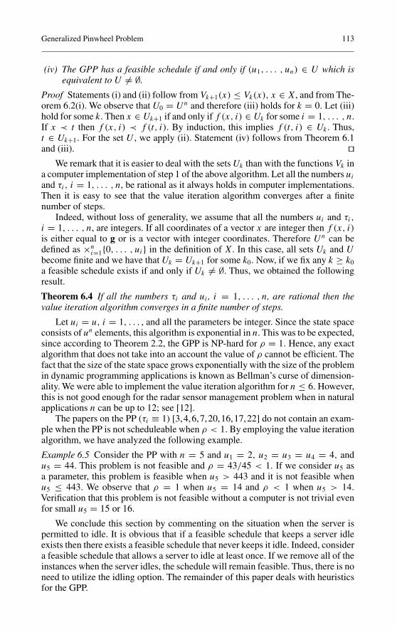
(iv) The GPP has a feasible schedule if and only if (u1, . . . , un) ∈ U which isequivalent to U �= ∅.

Proof Statements (i) and (ii) follow from Vk+1(x) ≤ Vk(x), x ∈ X, and from The-orem 6.2(i). We observe that U0 = Un and therefore (iii) holds for k = 0. Let (iii)hold for some k. Then x ∈ Uk+1 if and only if f (x, i) ∈ Uk for some i = 1, . . . , n.If x ≺ t then f (x, i) ≺ f (t, i). By induction, this implies f (t, i) ∈ Uk . Thus,t ∈ Uk+1. For the set U , we apply (ii). Statement (iv) follows from Theorem 6.1and (iii). ��

We remark that it is easier to deal with the sets Uk than with the functions Vk ina computer implementation of step 1 of the above algorithm. Let all the numbers ui

and τi, i = 1, . . . , n, be rational as it always holds in computer implementations.Then it is easy to see that the value iteration algorithm converges after a finitenumber of steps.

Indeed, without loss of generality, we assume that all the numbers ui and τi,i = 1, . . . , n, are integers. If all coordinates of a vector x are integer then f (x, i)is either equal to g or is a vector with integer coordinates. Therefore Un can bedefined as ×n

i=1{0, . . . , ui} in the definition of X. In this case, all sets Uk and Ubecome finite and we have that Uk = Uk+1 for some k0. Now, if we fix any k ≥ k0a feasible schedule exists if and only if Uk �= ∅. Thus, we obtained the followingresult.

Theorem 6.4 If all the numbers τi and ui , i = 1, . . . , n, are rational then thevalue iteration algorithm converges in a finite number of steps.

Let ui = u, i = 1, . . . , and all the parameters be integer. Since the state spaceconsists of un elements, this algorithm is exponential in n. This was to be expected,since according to Theorem 2.2, the GPP is NP-hard for ρ = 1. Hence, any exactalgorithm that does not take into an account the value of ρ cannot be efficient. Thefact that the size of the state space grows exponentially with the size of the problemin dynamic programming applications is known as Bellman’s curse of dimension-ality. We were able to implement the value iteration algorithm for n ≤ 6. However,this is not good enough for the radar sensor management problem when in naturalapplications n can be up to 12; see [12].

The papers on the PP (τi ≡ 1) [3,4,6,7,20,16,17,22] do not contain an exam-ple when the PP is not scheduleable when ρ < 1. By employing the value iterationalgorithm, we have analyzed the following example.

Example 6.5 Consider the PP with n = 5 and u1 = 2, u2 = u3 = u4 = 4, andu5 = 44. This problem is not feasible and ρ = 43/45 < 1. If we consider u5 asa parameter, this problem is feasible when u5 > 443 and it is not feasible whenu5 ≤ 443. We observe that ρ = 1 when u5 = 14 and ρ < 1 when u5 > 14.Verification that this problem is not feasible without a computer is not trivial evenfor small u5 = 15 or 16.

We conclude this section by commenting on the situation when the server ispermitted to idle. It is obvious that if a feasible schedule that keeps a server idleexists then there exists a feasible schedule that never keeps it idle. Indeed, considera feasible schedule that allows a server to idle at least once. If we remove all of theinstances when the server idles, the schedule will remain feasible. Thus, there is noneed to utilize the idling option. The remainder of this paper deals with heuristicsfor the GPP.

114 E.A. Feinberg, M.T. Curry

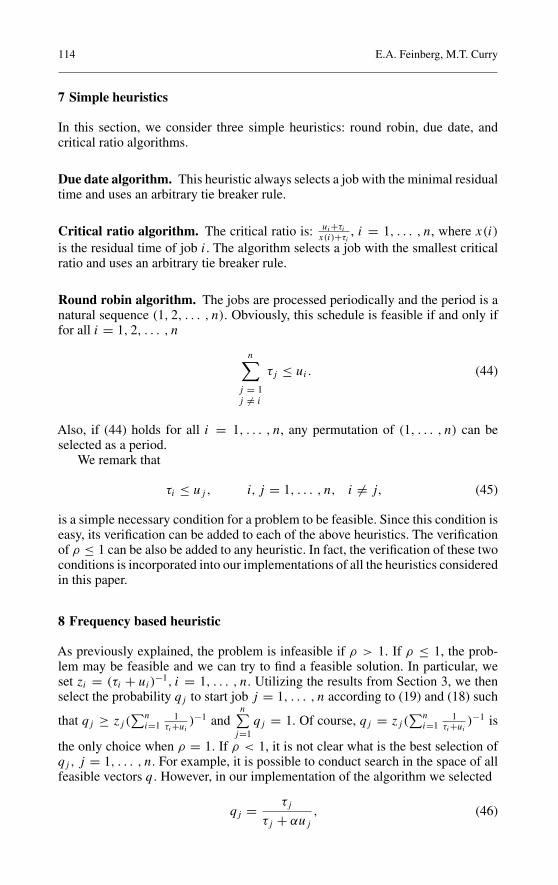
7 Simple heuristics

In this section, we consider three simple heuristics: round robin, due date, andcritical ratio algorithms.

Due date algorithm. This heuristic always selects a job with the minimal residualtime and uses an arbitrary tie breaker rule.

Critical ratio algorithm. The critical ratio is: ui+τi

x(i)+τi, i = 1, . . . , n, where x(i)

is the residual time of job i. The algorithm selects a job with the smallest criticalratio and uses an arbitrary tie breaker rule.

Round robin algorithm. The jobs are processed periodically and the period is anatural sequence (1, 2, . . . , n). Obviously, this schedule is feasible if and only iffor all i = 1, 2, . . . , n

n∑

j = 1j �= i

τj ≤ ui. (44)

Also, if (44) holds for all i = 1, . . . , n, any permutation of (1, . . . , n) can beselected as a period.

We remark that

τi ≤ uj , i, j = 1, . . . , n, i �= j, (45)

is a simple necessary condition for a problem to be feasible. Since this condition iseasy, its verification can be added to each of the above heuristics. The verificationof ρ ≤ 1 can be also be added to any heuristic. In fact, the verification of these twoconditions is incorporated into our implementations of all the heuristics consideredin this paper.

8 Frequency based heuristic

As previously explained, the problem is infeasible if ρ > 1. If ρ ≤ 1, the prob-lem may be feasible and we can try to find a feasible solution. In particular, weset zi = (τi + ui)

−1, i = 1, . . . , n. Utilizing the results from Section 3, we thenselect the probability qj to start job j = 1, . . . , n according to (19) and (18) such

that qj ≥ zj (∑n

i=11

τi+ui)−1 and

n∑

j=1qj = 1. Of course, qj = zj (

∑ni=1

1τi+ui

)−1 is

the only choice when ρ = 1. If ρ < 1, it is not clear what is the best selection ofqj , j = 1, . . . , n. For example, it is possible to conduct search in the space of allfeasible vectors q. However, in our implementation of the algorithm we selected

qj = τj

τj + αuj

, (46)

Generalized Pinwheel Problem 115

where α ≤ 1 is selected in a way that

n∑

i=1

τi

τi + αui

= 1. (47)

The intuitive justification for such a choice of q is the following. We are tryingto find a schedule in which the time between the completion and restart of job i isalways limited above by ui . Instead of this, we are finding a policy in the relaxationfor which the expectation of these times are limited by ui where ui ≤ ui . In otherwords, we decrease all ui to ui with the hope to extract the appropriate sequencefrom the strategy for which the expectations of these times are decreased. If wedecrease all ui proportionally, we have that ui = αui and there is a unique α forwhich (47) holds.

After qj , j = 1, . . . , n, are selected, they define a randomized stationary policyfor which the expected intervals between consequent instances of job i = 1, . . . , nare equal to ui . Since there is only one state, this randomized stationary policy isvery simple: jobs are selected independently and job i is always selected with theprobability qi, i = 1, . . . , n.

Our next step is to find a nonrandomized policy for which these expectationsare equal to ui . This can be done by using the time sharing approaches of Ross [23]and Altman and Shwartz [2]. Suppose we have a finite schedule seq1, . . . , seqN oflength N . Let Ni be the number of times the job i = 1, . . . , n has been executed,N = N1 + . . . + Nn. We select seqN+1 = argmax {qi − (Ni + 1)/(N + 1)} withan arbitrary tie breaker rule. We obtain the sequence seq1, seq2, . . . , seqk . . . .

Our initial conjecture was that in most cases, the sequence becomes periodic.Computational results showed that this is not the case. We introduce a heuristicwhereby we try to cut a feasible interval from the sequence seqk, seqk+1, . . . ,seqk+j that can be used as a period. In pseudo-code the algorithm is as follows:

Frequency based algorithm

1. Define sum to be the total number of iterations to be simulated.2. If either condition (45) does not hold or

∑ni=1

τi

τi+ui> 1, the problem is infea-

sible and the algorithm ends.3. If for each i = 1, . . . , n, the inequality (44) holds, the round robin sequence

1, 2, . . . , n, repeated an infinite number of times, forms a feasible sequenceand the algorithm ends.

4. Select zi ≥ τi

τi+ui, i = 1, . . . , n, such that

∑ni=1 zi = 1 (this can be imple-

mented in a number of ways, e.g. zi = τi(τi +ui)−1/

∑nj=1

τj

τj +uior zi = 1

τi+αui

with a constant α ≤ 1).5. Let qi = zi∑n

j=1 zj. i = 1, . . . , n. The value of qi is the probability that the next

selection is job i, i = 1, . . . , n.6. • Initialize N1, . . . , Nn and N to zero. The variable Ni counts the number

of times job i was performed. The variable N counts the total number ofjobs performed.

• Define a one-dimensional array called seq.This array will store the sequenceof jobs. The size of this array is the maximum length of the generated se-quence (sum). In other words, sum is an upper limit for N.

116 E.A. Feinberg, M.T. Curry

• Define a one-dimensional array called d. This array will store the differencebetween the theoretical frequency of executing job j = 1, . . . , n and theactual frequency. The dimension of v is n. Initialize di := 0, i = 1, . . . , n.

7. For (N = 1 to sum)Let j = argmaxi=1,... ,ndi . If there is a tie, implement an arbitrary tie breakingrule, e.g select j as the job with the maximal number for which the tie takesplace. Set:Nj := Nj + 1, di := qi − Ni

N, i = 1, . . . , n, seqN := j.

(The result is the array seq will now store the sequence of jobs performed toapproximate the probabilities prescribed by qi , i = 1, . . . , n. The remainderof the algorithm searches the array seq for a feasible fragment.)

8. Initialize variables a and b. Let a = M and b = a, where M is a “large”integer which is a small fraction of sum. The variable a is the beginning ofthe fragment being tested for feasibility and b is the end of this fragment.

9. Define a two-dimensional array called x. This array will be used to store theresidual values at each iteration. This array will have dimensions n by sum.Set xa

i = ui, i = 1, . . . , n.10. Increase b := b + 1 and calculate

xbi :=

{ui, if i = seqb;xi − τi, otherwise. i = 1, . . . , n.

11. If xbi < 0 at least for one i = 1, . . . , n, go to step 16.

12. If seqa �= seqb then go to step 11.13. If there is at least one job that has not been performed at least once between

iteration a and b inclusive, then go to step 11.14. Repeat the fragment l = seqa, seqa+1, . . . , seqb−1, seqb and check if the

resulted fragment l, l satisfies the condition that the sum of all job durations be-tween any two sequential completion and beginning of each job i = 1, . . . , nis not greater than ui. If yes then l, l, l, . . . is a feasible schedule (see the proofof Theorem 2.1 where the similar idea was used).

15. Increase a = a + 1 and set b = a.16. If a > sum − n, the algorithm stops without finding a feasible schedule.

Otherwise go to step 10.

9 Improved algorithms

The sets Ik introduced in Section 5 consist of the sequences of k jobs i1, . . . , iksuch that any two consecutive jobs are different. However, if k is large, some ofthese sequences cannot be continued to form periodic schedules. For example, if atotal length of all jobs in the finite sequence i ∈ Ik is longer than uj and the job j isabsent in this sequence, the sequence i cannot be continued as a feasible schedulefor the GPP.

First, we shall introduce the subsets Jk ⊆ Ik such that if i ∈ Jk we cannot sayimmediately that the sequence i cannot be continued as a feasible schedule for theGPP. By replacing the set of possible indices Ik in (34 – 37) with Jk we shall obtaintighter constraints that will possess the properties that the constraints for k + 1 aretighter that those for k.

Generalized Pinwheel Problem 117

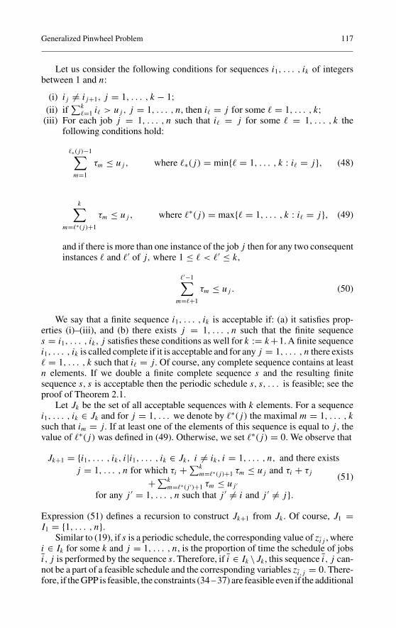
Let us consider the following conditions for sequences i1, . . . , ik of integersbetween 1 and n:

(i) ij �= ij+1, j = 1, . . . , k − 1;(ii) if

∑k�=1 i� > uj , j = 1, . . . , n, then i� = j for some � = 1, . . . , k;

(iii) For each job j = 1, . . . , n such that i� = j for some � = 1, . . . , k thefollowing conditions hold:

�∗(j)−1∑

m=1

τm ≤ uj , where �∗(j) = min{� = 1, . . . , k : i� = j}, (48)

k∑

m=�∗(j)+1

τm ≤ uj , where �∗(j) = max{� = 1, . . . , k : i� = j}, (49)

and if there is more than one instance of the job j then for any two consequentinstances � and �′ of j, where 1 ≤ � < �′ ≤ k,

�′−1∑

m=�+1

τm ≤ uj . (50)

We say that a finite sequence i1, . . . , ik is acceptable if: (a) it satisfies prop-erties (i)–(iii), and (b) there exists j = 1, . . . , n such that the finite sequences = i1, . . . , ik, j satisfies these conditions as well for k := k+1.A finite sequencei1, . . . , ik is called complete if it is acceptable and for any j = 1, . . . , n there exists� = 1, . . . , k such that i� = j. Of course, any complete sequence contains at leastn elements. If we double a finite complete sequence s and the resulting finitesequence s, s is acceptable then the periodic schedule s, s, . . . is feasible; see theproof of Theorem 2.1.

Let Jk be the set of all acceptable sequences with k elements. For a sequencei1, . . . , ik ∈ Jk and for j = 1, . . . we denote by �∗(j) the maximal m = 1, . . . , ksuch that im = j. If at least one of the elements of this sequence is equal to j , thevalue of �∗(j) was defined in (49). Otherwise, we set �∗(j) = 0. We observe that

Jk+1 = {i1, . . . , ik, i|i1, . . . , ik ∈ Jk, i �= ik, i = 1, . . . , n, and there existsj = 1, . . . , n for which τi + ∑k

m=�∗(j)+1 τm ≤ uj and τi + τj

+ ∑km=�∗(j ′)+1 τm ≤ uj ′

for any j ′ = 1, . . . , n such that j ′ �= i and j ′ �= j}.(51)

Expression (51) defines a recursion to construct Jk+1 from Jk . Of course, J1 =I1 = {1, . . . , n}.

Similar to (19), if s is a periodic schedule, the corresponding value of zij , wherei ∈ Ik for some k and j = 1, . . . , n, is the proportion of time the schedule of jobsi, j is performed by the sequence s. Therefore, if i ∈ Ik \Jk , this sequence i, j can-not be a part of a feasible schedule and the corresponding variables zi,j = 0. There-fore, if the GPP is feasible, the constraints (34 – 37) are feasible even if the additional

118 E.A. Feinberg, M.T. Curry

constraints zi,j = 0 when i ∈ Ik \Jk are imposed. This leads us to a tighter versionof the constraints (34 – 37) with the set Ik replaced with the smaller set Jk:

n∑

j = 1j �= ik

zij =n∑

j = 1j �= i1

(j, i1, . . . , ik−1) ∈ Jk

zj i , i = (i1, . . . , ik) ∈ Jk, (52)

∑

i=(i1,i2,... ,ik)∈Jk

n∑

j = 1j �= ik

zij τj = 1, (53)

∑

i = (i1, i2, . . . , ik) ∈ Jk

ik �= j

zij ≥ 1

uj + τj

, j = 1, . . . , n, (54)

zij ≥ 0, i ∈ Jk, j = 1, . . . , n, j �= ik. (55)

We observe that if i1, . . . , ik ∈ Jk for some k = 2, 3, . . . then i1, . . . , ik−1 ∈Jk−1. Therefore, Theorem 5.1 implies the following result.

Theorem 9.1 If z is a solution of the linear constraints (52 – 55) for some k ∈ N

then formula (38) defines a solution of the same linear constraints for k − 1.

We remark that a statement similar to Theorem 5.2 does not hold becauseit is possible that the sequences i1, . . . , ik and i2, . . . , ik+1 belong to Jk but thesequence i1, . . . , ik+1 does not belong to Jk+1. For example, consider the PP withn = 3 and ui = 2, i = 1, 2, 3. Then the sequences (1, 2) and (2, 1) are acceptablefor k = 2 but the sequence (1, 2, 1) is not acceptable. Therefore the constraints (52– 55) are tighter for higher values of k.

Next, we present the frequency based algorithms for k ∈ N

Frequency Based Algorithms FBk

1. Define sum to be the total number of iterations to be simulated.2. If either condition (45) does not hold or the system of constraints (52 – 55) is

infeasible, the GPP is infeasible and the algorithm ends.3. If for each i = 1, . . . , n the inequality (44) holds, the round robin sequence

1, 2, . . . , n repeated an infinite number of times, forms a feasible sequence andthe algorithm ends.

4. Select the vector (u1, . . . , un). This can be done iteratively by using varioussearch techniques. Similar to FB, we have implemented an approach when weselect ui = αui with α ≤ 1 being the minimal constant such that the systemof constraints (52 – 55) is feasible. The value of α can be found by bisection.Once the vector (u1, . . . , un) is defined, compute a solution zij of the systemof linear constraints (52 – 55). Set zi = ∑n

j = 1j �= ik

zij for all i = (i1 . . . ik) ∈ Jk.

Let Jk = {i ∈ Jk| zi > 0}.5. Set qij = zij /zi for all i ∈ Jk and for all j = 1, . . . , n, j �= ik . If the transition

probabilities qij define a Markov chain with more than one recurrent class [18,Algorithm 1], a feasible schedule is not found.

Generalized Pinwheel Problem 119

6. • Initialize Nij , Ni , and N to zero, where i = (i1 . . . ik) ∈ Jk, j = 1, . . . , n,and j �= ik. The variable Ni and Nij respectively count the number of timeseach of the strings i and (i1 . . . ikj) were observed. The variable N countsthe total number of jobs performed.

• Define a one-dimensional array called seq.This array will store the sequenceof jobs. The size of this array is the maximum length of the generated se-quence (sum). In other words, sum is an upper limit for N. Initialize N = k

and set seq = i for some i = (i1 . . . ik) ∈ Jk. Let M be the number of ele-ments in Jk.

• Define a two-dimensional array called d. This array will store the differencebetween the theoretical frequency of executing job j = 1, . . . , n at statesi ∈ Jk and the actual frequency. The dimensions of v are M by n. Initializeall elements of d equal to 0.

• Define a two-dimensional array called r . This array will be used to store theresidual values at each iteration. This array will have dimensions n by sum.

• Select any i ∈ Jk. Let i = (i1 . . . ik).7. For (N = 1 to sum)

Let j = argmax{j=1,... ,n;j �=ik}dij . If there is a tie, implement an arbitrary tiebreaking rule, e.g select j as the job with the maximal number for which the tietakes place. Set: Nij := Nij + 1, Ni := Ni + 1, i := (i2 . . . ikj), seqN := j,

dij := qij − Nij

Ni, j = 1, . . . , n. The remainder of the algorithm searches the

array seq for a feasible fragment as is in the frequency based algorithm, Steps8 – 16, described in Section 8.

We remark that, though the transition probabilities calculated at step 5 theoret-ically can define a Markov chain with multiple recurrent classes, we have neverexperienced this in the thousands of calculations performed.

Using the heuristics FBk we can formulate the second exact algorithm as fol-lows (the first exact algorithm is the value iteration algorithm from Section 6).

1. Apply the frequency based algorithm from Section 8. Stop if a feasible scheduleis found or the problem is detected to be infeasible.

2. Set k = 1, Jk = {1, . . . , n}, and apply the frequency based algorithm FBkfrom Section 9. Stop if a feasible schedule is found or the problem is detectedto be infeasible.

3. Increase the value of k by 1. Calculate the set Jk by using the recursion (51).If Jk = ∅ then the problem is infeasible. Otherwise, let Ck be the subset ofthe complete sequences of Jk. Sequentially double each i sequence in Ck. Ifthe sequence i, i satisfies the condition that the time between all consecutiveinstances of job j = 1, . . . , n is not greater than uj , then i, i, i, . . . is a feasibleperiodic schedule. If the feasible schedule is not found, go to Step 2.

Since, according to Theorem 2.2, the GPP is NP-hard, the latter algorithm isnot efficient. Its convergence follows from the following arguments. Leaving apartthe possibility that the heuristics at Steps 1 or 2 solve the problem, consider thefollowing two possibilities: (i) the problem is feasible, and (ii) the problem is notfeasible. If the problem is feasible and its shortest (in terms of the number of jobsin it) period consists of k jobs, it will be detected at Step 3 when the appropriateelement of Ck is doubled unless a feasible schedule has been found earlier. If the

120 E.A. Feinberg, M.T. Curry

problem is infeasible, it is easy to see from the proof of Theorem 2.1 that the setJk will become empty for large k.

We remark than among all FBk algorithms with k > 1, the case k = 1 appearsto be the most interesting in terms of its applicability. The reason is that FBkalgorithms require solutions of linear constraints with up to n(n − 1)k variables.However, as Corollary 5.3 implies, the constraints (52 – 55) become tighter whenthe set Jk is smaller than the set Ik. For reasonable n this happens with relativelylarge values of k. For example, typically I2 = J2 and FB2 probably should notsignificantly outperform FB1. This is the reason we implemented FBk heuristicsfor k = 0 and k = 1. Our simulations indicated that FB1 solves roughly 5% casesmore than FB (k = 0).

10 Simulation results

We provide simulation results for one of the two data sets considered in [12] for theradar sensor management problem. We conducted a simulation of the job durationsof 0.0587, 0.175, 0.223, and 0.299 that were randomly and independently assignedto each of the jobs with the probability 1

4 . Revisit times of 1, 3, or 4 were alsorandomly and independently assigned to each of the jobs with the probability 1

3 .Each simulation of 1000 cases has been conducted for n = 4, 5, . . . , 12. The RR,CR, FB, and FB1 were applied to the simulated data for comparison. It was foundthat the frequency based FB algorithm outperformed significantly both the criticalratio and round robin algorithms. The frequency based algorithm for k = 1, FB1,demonstrated even better results than FB. It found a feasible schedule in a higherpercentage of cases. In addition, FB1 detected more cases when the problem isinfeasible. For the RR, CR, and FB heuristics we used the condition ρ > 1 todetect the cases that cannot be feasible. The FB1 heuristic checks the feasibilityof the constraints (27 – 30) which is a more powerful criterion. The results of thissimulation are shown in table 9.1 below. According to these results, FB1 is betterthan FB and FB outperforms CR. Of course, RR is the most primitive heuristic.

Table 9.1 Simulation results

#jobs RR CR FB FB1 RR CR FB FB1 FB FB14 100 100 100 100 92.4 100 100 100 0 05 92.4 100 100 100 92.4 100 100 100 0 06 55.3 97.2 100 100 55.3 97.2 100 100 0 07 22.5 89.1 98.4 99.1 22.5 89.1 98.4 99.3 0 .28 10.3 76.7 92.7 95.4 12.9 79.3 95.3 98.6 2.6 3.29 3.4 53.6 79.5 83.5 8.8 59.0 84.9 91.0 5.4 7.510 2.7 27.3 62.3 64.5 16.2 40.8 75.8 81.2 13.5 16.711 2.3 18.2 41.6 44.6 32.4 48.3 71.7 79.8 30.1 35.212 2 8.1 22.3 25.3 47.8 53.9 68.1 78.5 45.8 53.2

Percentage of scheduled *Percentage of cases Percentage of casescases using (RR), (CR), where a solution could that were found to be(FB), and (FB1). be found using (RR), infeasible using

(CR), (FB), and (FB1). (FB) and (FB1).*Includes the case when infeasible cases are detected.

Generalized Pinwheel Problem 121

11 Conclusions and open questions

This paper studied a Generalized Pinwheel Problem (GPP) which is to find afeasible infinite sequence of jobs from a set of n recurring jobs with durations τi,i = 1, . . . , n. Each time job i is completed, it should be restarted within ui units oftime. According to Theorem 2.2, his problem is NP-hard, at least when the densityρ equals 1. When all τi = 1, this problem becomes the Pinwheel Problem (PP)studied in [3,4,6,7,20,16,17,22].

The GPP can be applied to many problems that involve repetitive executionsof tasks with non-uniform durations and deadlines. The examples of applicationsinclude: the radar sensor management, machine refuelling, database support, andinspection scheduling problems.

We have shown that a feasible GPP has a feasible periodic schedule. In thispaper we established a link between relaxed versions of the GPP and constrainedundiscounted Semi-Markov Decision Process. By using this link, we developedrelaxations of the GPP and formulated the so-called frequency based algorithmsthat outperform other known heuristics. These relaxations become tighter whenthe parameter k, that is relevant to the memory used by the algorithms, increases.The simplest relaxation for k = 0 implies that ρ ≤ 1 is a necessary condition for aproblem to be feasible. Other relaxations, for k = 1, 2 . . . provide more accuratenecessary conditions that may detect that the problem is not feasible in some caseswhen ρ ≤ 1. We also provided computational results that illustrate the efficiencyof the introduced algorithms.

In general, a feasible schedule, if it exists, can be presented as a function of avector of residual times. We have developed a value iteration algorithm based onDynamic Programming. Though this algorithm converges, it is computationallyintractable for large n, which is consistent with NP-complexity of the GPP. Theimplementation of this algorithm allowed us to construct the example of an infea-sible PP with ρ < 1. We also showed in this paper that, unlike the PP, the GPP canbe infeasible when ρ is small.

There are several interesting open questions for the PP and for the GPP. WhenHolte et al [16] introduced the PP, they stated without the proof that the PP isNP-hard when ρ = 1. However their detailed paper [17] did not mention thisfact. Chan and Chin [7] provided a polynomial algorithm that always constructsa schedule for a PP with ρ ≤ 0.7. Nothing is known about the complexity of PPwhen ρ > 0.7. It would be interesting to have the boundaries on ρ when the PPis always feasible, when it is polynomial, and when it is NP-hard. The interestingquestion is whether the GPP is NP-hard for ρ < 1 and whether it is possible todevelop a polynomial algorithm for the GPP when ρ ≤ α for some α < 1. Ofcourse, an interesting question is whether it is possible to develop better heuristicsthan the frequency based algorithms.

Acknowledgements This research was partially supported by NSF grant DMI-0300121 and bya research grant from NYSTAR (New York State Office of Science, Technology and AcademicResearch). The authors are grateful to Michael Bender, Daniel Huang, Theodore Koutsoudis, andJoel Bernstein for valuable discussions relevant to this paper.

122 E.A. Feinberg, M.T. Curry

References

1. Avrachenkov, K.E., Filar, J., Haviv, M.: Singular perturbations of Markov chains and decisionprocesses. In: Feinberg, E.A., Adam Shwartz, (eds.) Handbook of Markov Decision Pro-cesses, Kluwer, Boston, pp 113–150, 2002

2. Altman, E., Shwartz, A.: Time-sharing policies for controlled Markov chains. OperationsResearch 41, 1116–1124 (1993)

3. Baruah, S.K., Lin, S.-S.: Pfair scheduling of generalized pinwheel task systems. IEEE Trans-actions on Computers 47(7), 812–816 (1998)

4. Baruah, S.K., Howell, R.R., Rosier, L.E.: Feasibility problems for recurring tasks on oneprocessor. Theoretical Computer Science 118, 3–20 (1993)

5. Borkar, V.S., Ejov, V., Filar, J.A.: Directed graphs, Hamiltonicity and doubly stochasticmatrices. Random Structures and Algorithms 25, 376–395 (2004)

6. Chan, M.Y., Chin, F.: General schedulers for the pinwheel problem based on double integerreduction. IEEE Transactions on Computers 41, 755–768 (1992)

7. Chan, M.Y., Chin, F.: Schedulers for larger classes of pinwheel instances. Algorithmica 9,425–462 (1993)

8. Ejov, V., Filar, J.A., Nguyen., M.: Hamiltonian cycles and singularly perturbed Markovchains. Math. Oper. Res. 29, 114–131 (2004)

9. Feinberg, E.A.: Constrained semi-Markov decision process with average rewards. ZORMath. Meth. Oper. Res. 39, 257–288 (1994)

10. Feinberg, E.A.: Total reward criteria. In: Feinberg E.A., Adam Shwartz (eds.) Handbook ofMarkov Decision Processes, Kluwer, Boston, 175–207, 2002

11. Feinberg, E.A.: Constrained discounted Markov decision processes and Hamiltonian cycles.Math. Oper. Res. 25, 130–140 (2000)

12. Feinberg, E.A., Bender, M.A., Curry, M.T., Huang, D., Koutsoudis, T., Bernstein, J.L.: Sen-sor resource management for an airborne early warning radar. Proceedings of the SPIE-TheInternational Society for Optical Engineering, Signal and Data Processing of Small Targets4728, 145–156 (2002)

13. Filar, J.A., Guo, X.: Linear program for communicating MDPs with multiple constraints.In: Z. Hou et al. (eds.) Markov Processes and Controlled Markov Chains, Kluwer AcademicPublishers, Netherlands, pp 245–254, 2002

14. Filar, J.A., Krass, D.: Hamiltonioan cycles and Markov chains. Math. Oper. Res. 25, 223–237(1994)

15. Garey, M.R., Johnson, D.S.: Computers and intractability: a guide to the theory ofNP-completeness. W. H. Freeman, San Francisco, 1979

16. Holte, R., Rosier, L., Tulchinsky, I.,Varvel, D.: The Pinwheel:A realtime scheduling problem.Proceedings of the Annual Hawaii International Conference on System Sciences, 693–702(1989)

17. Holte, R., Rosier, L., Tulchinsky, I., Varvel, D.: Pinwheel scheduling with two distinct num-bers. Theoretical Computer Science 100, 105–135 (1992)

18. Kallenberg, L.C.M.: Classification problems in MDPs. In: Hou, Z., Filar, J.A., Chen,A. (eds)Markov Processes and Controlled Markov Chains, Kluwer, Dordrecht, pp 151–165, 2002

19. Leung, J.Y.T.: A new algorithm for scheduling periodioc, real time tasks. Algorithmica 4,209–219 (1989)

20. Lin, S.S., Lin, K.J.: A pinwheel scheduler for three distinct numbers with a tight schedula-bility bound. Algorithmica 19, 411–426 (1997)

21. Puterman, M.I.: Markov decision processes: discrete stochastic dynamic programming. JohnWiley & Sons, New York, 1994

22. Romer, T.H., Rosier, L.E.: An algorithm reminiscent of Euclidean-gcd for computing afunction related to pinwheel scheduling. Algorithmica 17, 1–10 (1997)

23. Ross, K.W.: Randomized and past-dependent policies for Markov decision processes withmultiple constraints. Operations Research 37, 474–477 (1989)

24. Strauch, R.E.: Negative dynamic programming. The Annals of Mathematical Statistics 37,871–890 (1966)