Microarray Experimental Design Workshop

Ann Hess

Center for Bioinformatics and

Department of Statistics

hess@stat.colostate.edu

2

Welcome

� Experimental design is an important step when planning a microarray experiment.

� A good design will allow to make the most of your resources.

� This workshop will discuss sample size and allocation of samples to arrays, but not probe selection or array layout.

3

Overview

1. Getting Started

2. Pooling

3. Blocking

4. Sample Size Determination

5. Designs for “two-color” arrays

6. Conclusions

4

1. Getting Started

� The study objective drives the experimental design and analysis.

� Different types of arrays are available.

� There are multiple sources of variation and different types of replication.

� Steps should be taken to reduce technical variability and avoid confounding.

� Basic design principles should be used.

5

Study Objectives

� Class Comparison: goal is to determine whether

gene expression profiles differ among samples from different classes and identify which genes are differentially expressed between classes.

� Class Prediction: goal is to develop a statistical model that can predict which class a new specimen belongs to based on its expression profile.

� Class Discovery: goal is to identify novel sub-types of specimens within a population.

� Pathway Analysis: goal is to identify genes that are co-regulated or which occur in the same biochemical pathway.

� Other: ????

6

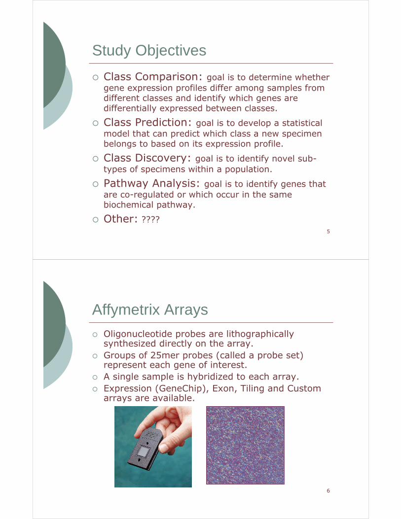
Affymetrix Arrays

� Oligonucleotide probes are lithographically synthesized directly on the array.

� Groups of 25mer probes (called a probe set) represent each gene of interest.

� A single sample is hybridized to each array.

� Expression (GeneChip), Exon, Tiling and Custom arrays are available.

7

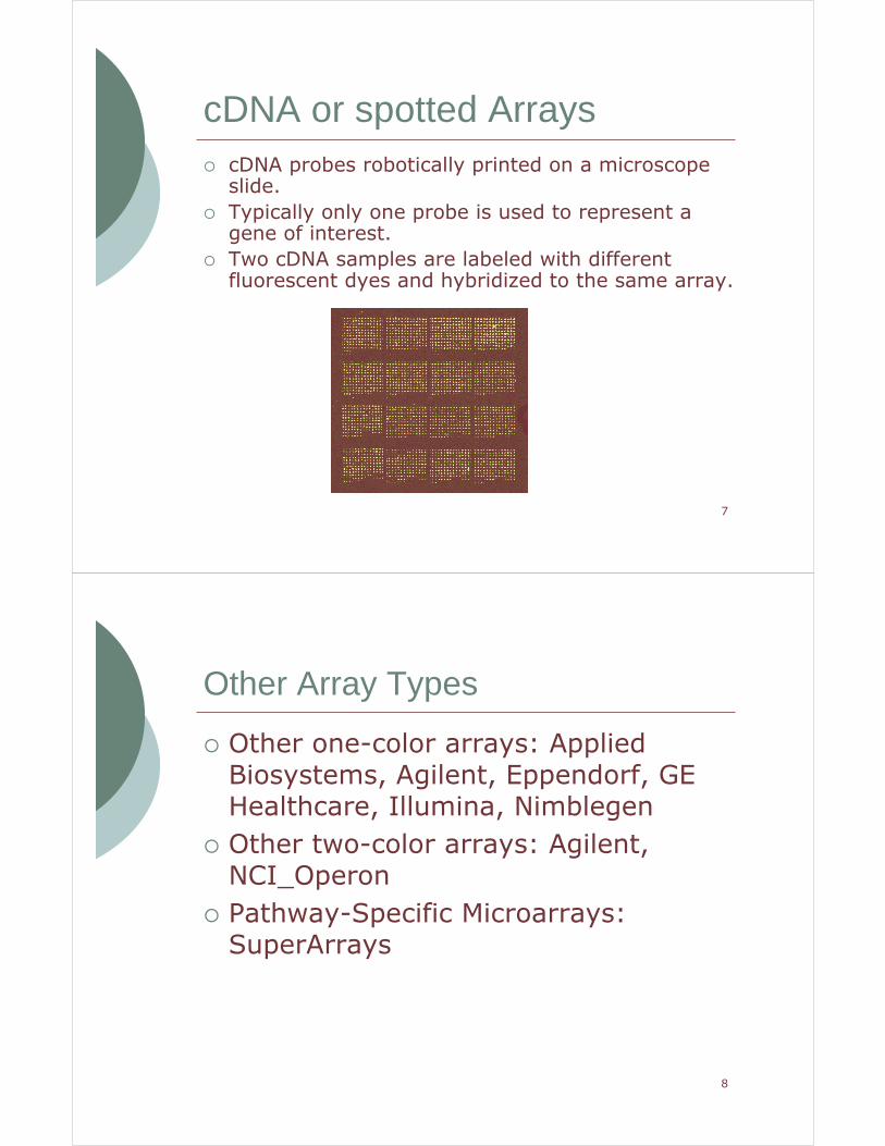
cDNA or spotted Arrays� cDNA probes robotically printed on a microscope

slide.

� Typically only one probe is used to represent a gene of interest.

� Two cDNA samples are labeled with different fluorescent dyes and hybridized to the same array.

8

Other Array Types

� Other one-color arrays: Applied Biosystems, Agilent, Eppendorf, GE Healthcare, Illumina, Nimblegen

� Other two-color arrays: Agilent, NCI_Operon

� Pathway-Specific Microarrays: SuperArrays

9

Choosing an Array Type

� Study Objective: Is the study focused on gene expression or something else?

� Availability: Is there a manufactured array for your species of interest?

� Cost: What is the cost per array?

� Performance: Microarray Quality Control Study (MAQC) study compares the performance of many manufactured arrays.

� Genes of interest: Are your genes of interest represented on the array?

10

Experiment or Observational Study

� In an experiment, the explanatory variable is randomly assigned to subjects.

� Example: Rats are randomly assigned to either be induced with breast cancer or to serve as controls.

� In an observational study, we just observe differences between groups.

� Example: Blood samples from women with breast cancer are compared to healthy controls.

� Experiments allow us to draw causal conclusions.

� For observational studies, it is important to consider extraneous differences between groups being compared.

11

Biological and Technical Replicates

� Biological replication: multiple cases per group are studied.

� Technical replication: RNA samples from one case are hybridized to multiple arrays.

� Biological replication is essential.

� Technical replication (with independently labeled aliquots from a single RNA sample) provides information about the variability of the labeling, hybridization and quantification processes.

12

Sources of VariationBiological Variation:

Technical Variation:

• Between subjects within the same treatment• Between specimens from the same subject

• Between arrays for the same RNA sample• Between replicate spots on the same array

13

Sources of Variation

� Zakharkin et al. (2005) examined sources of variation in Affymetrix microarray experiments using mammary gland samples from 8 rats.

� RNA samples from each rat were split to assess variation arising at the labeling and hybridization steps.

� The authors found that the greatest source of variation was biological variation, followed by residual error and finally variation due to labeling.

14

Sources of Variation

� Han et al. (2004) examined sources of variation in Affymetrix microarray experiments using liver samples from mice.

� “Nine GeneChips representing RNA from 3 different animals…were assayed 3 times on 3 different days.”

� The authors found the greatest source of variation was residual error, followed by biological variation and finally variation due to day-to-day effects.

15

Reducing Technical Variability and Avoiding Confounding

� Attempts should be made to reduce technical variability and avoid confounding in a study!

� If possible, sample collection, RNA extraction and labeling of all samples in an experiment should be performed by the same individual at the same time of day using the same protocol and reagents.

� If samples become available at different times, consider freezing and processing together.

� If possible, arrays should be used from a single manufacturing batch and processed by one technician on the same day.

� For large studies (where this is not possible) randomize and consider blocking.

16

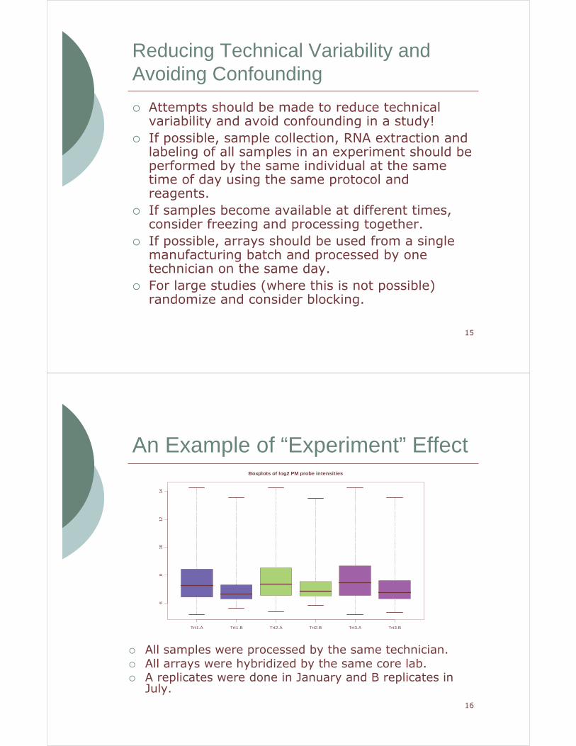
An Example of “Experiment” Effect

� All samples were processed by the same technician. � All arrays were hybridized by the same core lab.� A replicates were done in January and B replicates in

July.

Trt1.A Trt1.B Trt2.A Trt2.B Trt3.A Trt3.B

68

1012

14

Boxplots of log2 PM probe intensities

17

Basic Design Principles

� Randomization: randomize as much as possible to protect against unanticipated biases.

� Replication: more (biological) replicates will generally correspond to higher power.

� Balance: equal number of replicates per treatment is usually desirable.

� Pooling: can be used to reduce biological variability.

� Blocking: can be used to reduce experimental variability.

18

2. Pooling

� If not enough RNA can be obtained from a single subject, then pooling or amplification is necessary.

� Here we consider pooling for the purpose of reducing the effects of biological variation.

� With pooling, sample size can be increased without purchasing more arrays.

� Kendziorski et al. (2005) examine the effect of pooling biological samples in microarray experiments.

19

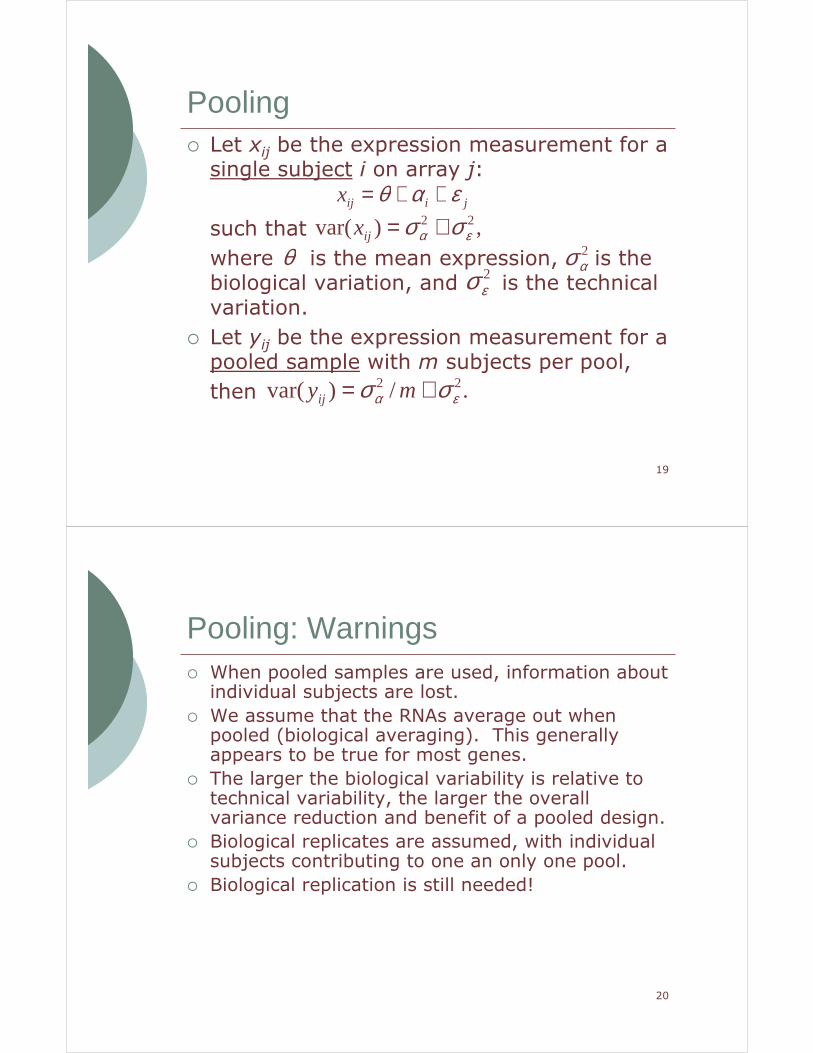
Pooling� Let xij be the expression measurement for a single subject i on array j:

such that

where is the mean expression, is the biological variation, and is the technical variation.

� Let yij be the expression measurement for a pooled sample with m subjects per pool,

then

jiijx εαθ ++=,)var( 22

εα σσ +=ijxθ 2

ασ2εσ

./)var( 22εα σσ += myij

20

Pooling: Warnings� When pooled samples are used, information about

individual subjects are lost.

� We assume that the RNAs average out when pooled (biological averaging). This generally appears to be true for most genes.

� The larger the biological variability is relative to technical variability, the larger the overall variance reduction and benefit of a pooled design.

� Biological replicates are assumed, with individual subjects contributing to one an only one pool.

� Biological replication is still needed!

21

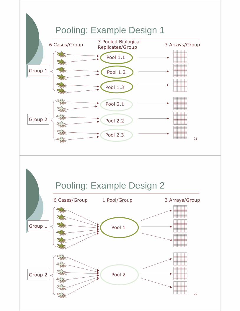
Pooling: Example Design 13 Pooled Biological Replicates/Group

Pool 1.1

Pool 2.1

Pool 1.2

Pool 1.3

Pool 2.2

Pool 2.3

6 Cases/Group 3 Arrays/Group

Group 1

Group 2

22

Pooling: Example Design 21 Pool/Group6 Cases/Group 3 Arrays/Group

Group 1

Group 2

Pool 1

Pool 2

23

Pooling: Comparing Designs

� In Design 1, we use 6 cases/group to form 3 distinct pooled samples/group which are hybridized to 3 arrays.

� In Design 2, we use 6 cases/group to form a single pooled sample/group which is divided and hybridized to 3 arrays.

Design #1 is recommended because we have biological replicates.

- 3 Biological Replicates/Group

- 3 Technical Replicates/Group

24

Pooling

� Pooling can be beneficial when:� identifying differential expression is the only goal,

� when biological variation is high relative to technical variation and

� when biological subjects are inexpensive relative to array cost.

� Pooling was found to be most helpful when the number of arrays was small.

25

3. Blocking

� Blocking can be used to reduce variability.

� Experimental units are grouped such that the variability of cases within the groups (blocks) is less than that among all cases prior to grouping (blocking).

� Treatments are compared with one another within groups of cases so that the differences between the treatments are not confused with large differences between cases.

26

Blocking: Criteria

� Four major criteria frequently used to block experimental units are:

� Proximity (neighboring field plots)

� Physical characteristics (age or weight)

� Time

� Management of tasks in the experiment

� Classical blocking practice had its origins in agricultural field experiments where contiguous plots were considered a block.

� Another classic example is the use of animal litter as the blocking variable.

27

Blocking: Example 1

� Researchers on campus were interested in identifying genes that were differentially expressed between osteoarthritic and control joints in horses. In addition to the treatment they were also interested in the effect due to tissue.

� There are a total of four conditions:

- Osteoarthritic Deep

- Osteoarthritic Superficial

- Control Deep

- Control Superficial

28

Blocking: Example 1

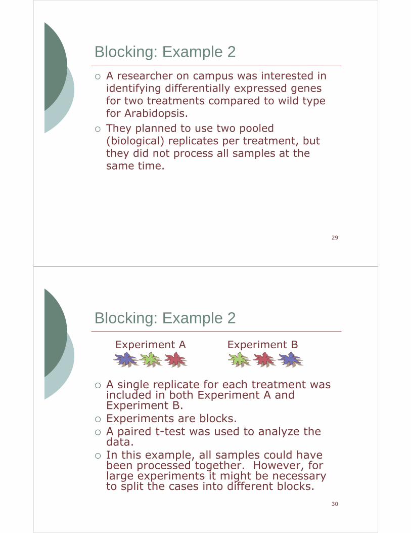
Osteoarthritic joint Control joint

� For each of six healthy horses, one joint was randomly selected and induced with osteoarthritis while the other joint served as a control.

� Deep and superficial tissue samples were taken from each joint.

� Horses were used as blocks.

� Since each condition was measured within each block, a randomized complete block design was used.

� A mixed model was used to analyze the data.

29

Blocking: Example 2� A researcher on campus was interested in identifying differentially expressed genes for two treatments compared to wild type for Arabidopsis.

� They planned to use two pooled (biological) replicates per treatment, but they did not process all samples at the same time.

30

Blocking: Example 2

� A single replicate for each treatment was included in both Experiment A and Experiment B.

� Experiments are blocks.� A paired t-test was used to analyze the data.

� In this example, all samples could have been processed together. However, for large experiments it might be necessary to split the cases into different blocks.

Experiment A Experiment B

31

4. Sample Size

� Perhaps the most difficult aspect of microarray experimental design is deciding how many biological replicates should be used.

� More replicates will generally correspond to higher power.

� In practice, the number of replicates will be determined (at least in part) by budget.

� Pavlidis et al. (2003) recommend using 5 or more replicates.

32

Sample Size

� For this discussion, we assume that the goal of the experiment is to identify differentially expressed genes.

� Then the null hypothesis is “equal expression” between two (or more) groups and the alternative is “differential expression”.

� Power is defined as the probability of rejecting a null hypothesis that is actually false. Higher power indicates an increased ability to detect differentially expressed genes.

33

Sample Size

� If we are interested in detecting differentially expressed genes, then we are testing for a difference between treatment group means.

� The required number of replicates depends on:

� Variance

� Size of the difference between two means

� Significance level of the test (alpha)

� Power of the test

34

Sample Size

� For microarray experiments, thousands of hypotheses will be tested because each gene corresponds to one or more hypothesis tests.

� This effects the sample size determination in the following ways:� Different genes will have different levels of variability.

� There is dependence between genes.� A multiple testing adjustment should be used, so our stated significance level needs to be adjusted.

35

Sample Size: Approaches

� Approaches to sample size have been developed specifically for microarrays:

� Simple Approach

� ssize Package

� Power Atlas Method

� Zien Simulation Approach

� SimArray

36

Sample Size: COPD Data

� A comparison of lung tissue from 18 smokers with severe emphysema and 12 smokers with mild or no emphysema was performed.

� This study provides insight into the pathogenesis of chronic obstructive pulmonary disease (COPD).

� The Affymetrix HG-U133A GeneChip was used for the study. This chip type has 22,283 probe sets.

� This data is publicly available from GEO as data set GDS737.

37

Sample Size: Simple Approach

� Use a statistical package (SAS, R, minitab) to calculate power for a specified sample size based on a t-test or one-way ANOVA model.

� Required Input

� standard deviation

� power

� significance level (alpha value)

� difference between means (log2 fold change)

� Use available data to estimate variance.

38

Sample Size: Simple Approach

� Using the COPD data, we use R/Bioconductor to calculate RMA expression values for the control group.

� Then calculate the standard deviation of the expression values. The 75th percentile is 0.296.

� We choose� an alpha value of 0.0001 (because we assume a

multiple testing adjustment will be performed)

� difference between means (log2FC) =+/-1

� Using SAS Proc Power to calculate the power for a two-sided t-test with 10 arrays per group, the power is calculated to be 0.979.

39

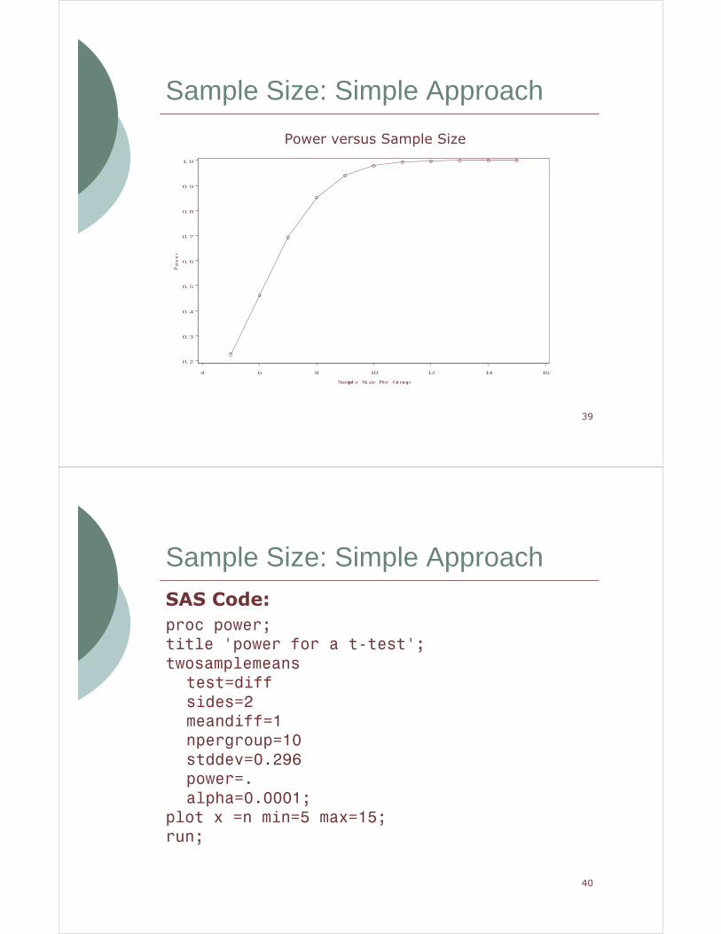
Sample Size: Simple Approach

4 6 8 10 12 14 16

Sampl e Si ze Per Group

0. 2

0. 3

0. 4

0. 5

0. 6

0. 7

0. 8

0. 9

1. 0

Power versus Sample Size

40

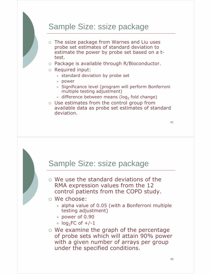
Sample Size: Simple Approach

proc power;

title 'power for a t-test';

twosamplemeans

test=diff

sides=2

meandiff=1

npergroup=10

stddev=0.296

power=.

alpha=0.0001;

plot x =n min=5 max=15;

run;

SAS Code:

41

Sample Size: ssize package

� The ssize package from Warnes and Liu uses probe set estimates of standard deviation to estimate the power by probe set based on a t-test.

� Package is available through R/Bioconductor.

� Required input:� standard deviation by probe set

� power

� Significance level (program will perform Bonferroni multiple testing adjustment)

� difference between means (log2 fold change)

� Use estimates from the control group from available data as probe set estimates of standard deviation.

42

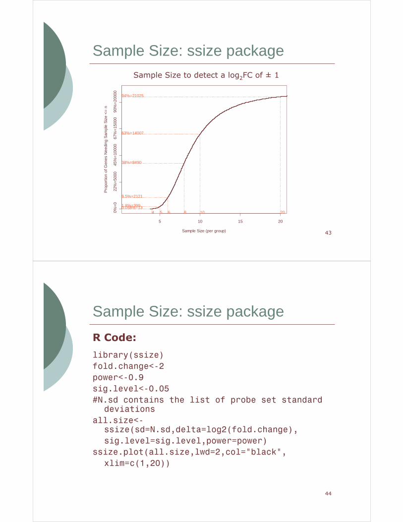
Sample Size: ssize package

� We use the standard deviations of the RMA expression values from the 12 control patients from the COPD study.

� We choose:� alpha value of 0.05 (with a Bonferroni multiple testing adjustment)

� power of 0.90

� log2FC of +/-1

� We examine the graph of the percentage of probe sets which will attain 90% power with a given number of arrays per group under the specified conditions.

43

Sample Size: ssize package

5 10 15 20

Sample Size (per group)

Pro

port

ion

of G

enes

Nee

ding

Sam

ple

Siz

e <

= n

0%

=0

22%

=50

00 4

5%=

1000

0 6

7%=

1500

0 9

0%=

2000

0

40.058%=13

5

1.8%=399

6

9.5%=2121

8

38%=8490

10

63%=14007

20

94%=21025

Sample Size to detect a log2FC of ± 1

44

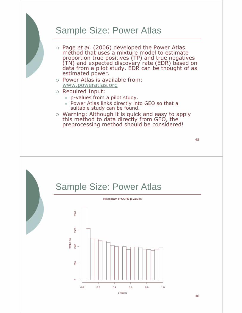
Sample Size: ssize package

library(ssize)

fold.change<-2

power<-0.9

sig.level<-0.05

#N.sd contains the list of probe set standard deviations

all.size<-ssize(sd=N.sd,delta=log2(fold.change),

sig.level=sig.level,power=power)

ssize.plot(all.size,lwd=2,col="black",

xlim=c(1,20))

R Code:

45

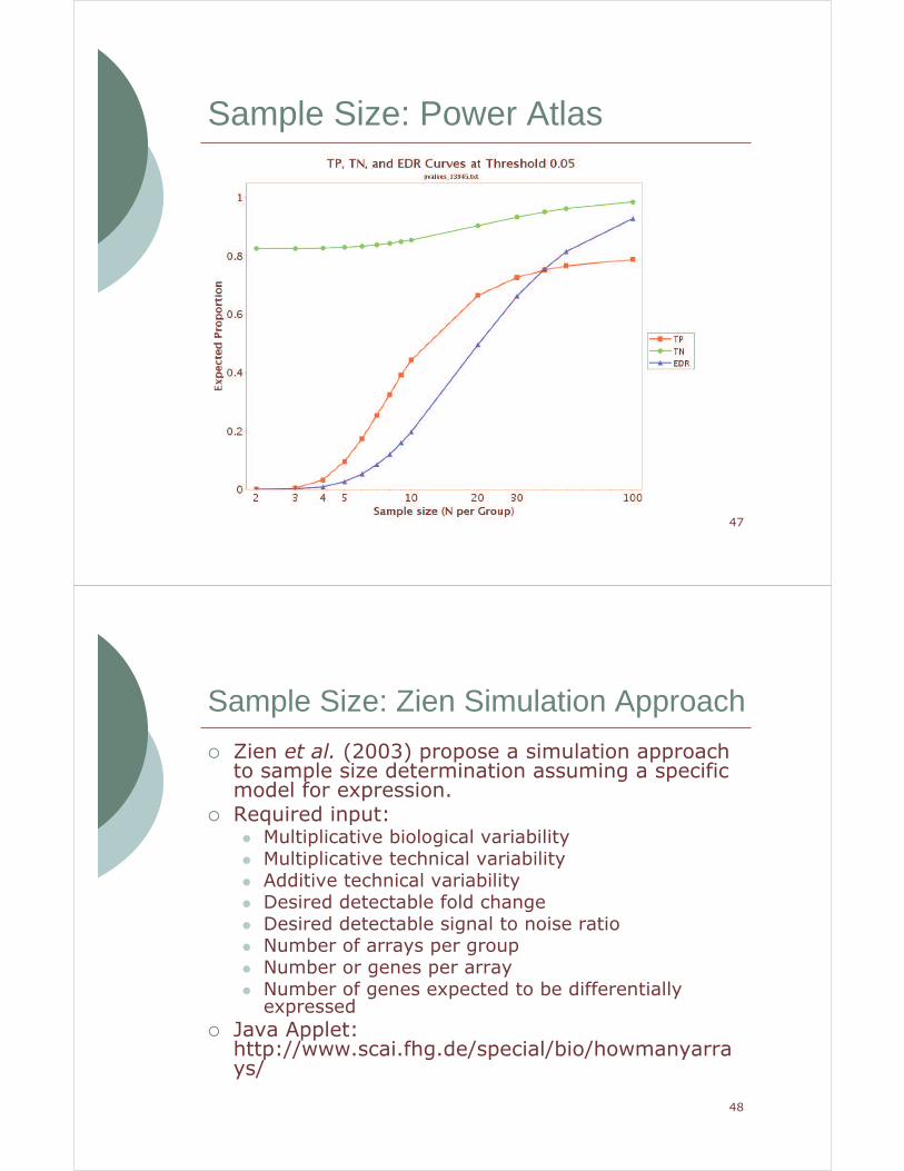
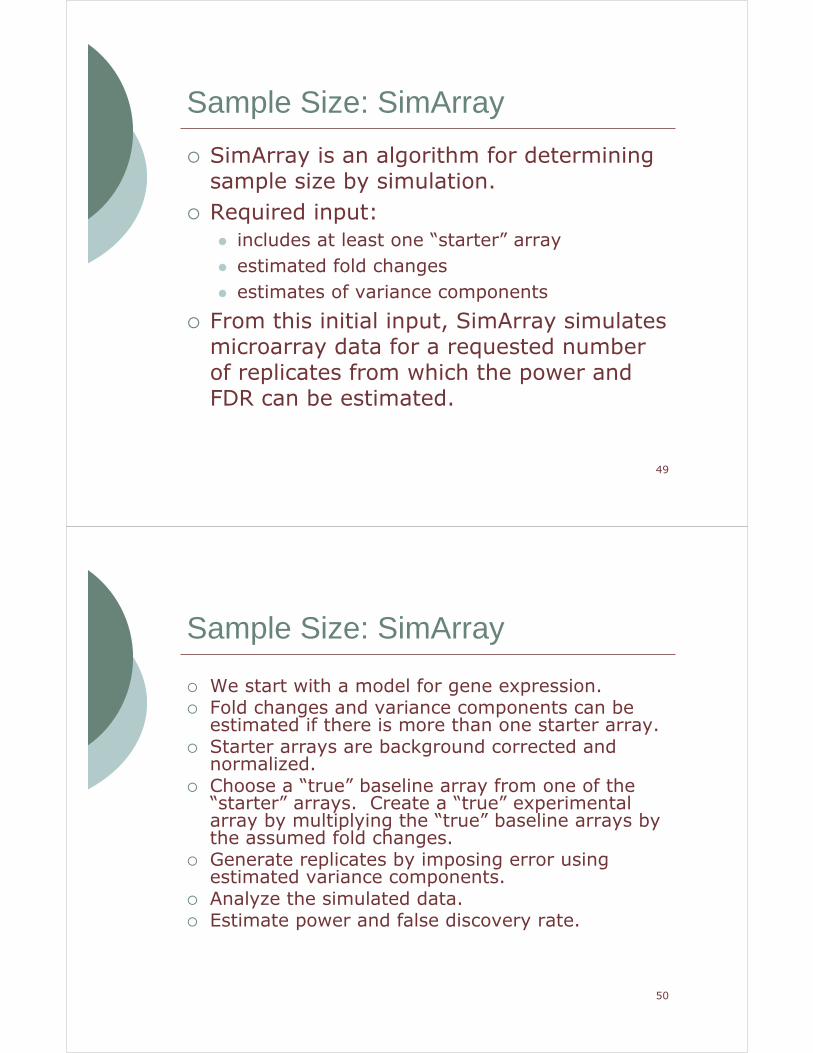
Sample Size: Power Atlas

� Page et al. (2006) developed the Power Atlas method that uses a mixture model to estimate proportion true positives (TP) and true negatives (TN) and expected discovery rate (EDR) based on data from a pilot study. EDR can be thought of as estimated power.

� Power Atlas is available from: www.poweratlas.org

� Required Input:� p-values from a pilot study.� Power Atlas links directly into GEO so that a

suitable study can be found.

� Warning: Although it is quick and easy to apply this method to data directly from GEO, the preprocessing method should be considered!

46

Sample Size: Power AtlasHistogram of COPD p-values

p-values

Fre

quen

cy

0.0 0.2 0.4 0.6 0.8 1.0

050

010

0015

0020

00

47

Sample Size: Power Atlas

48

Sample Size: Zien Simulation Approach

� Zien et al. (2003) propose a simulation approach to sample size determination assuming a specific model for expression.

� Required input:� Multiplicative biological variability� Multiplicative technical variability� Additive technical variability� Desired detectable fold change� Desired detectable signal to noise ratio� Number of arrays per group� Number or genes per array� Number of genes expected to be differentially

expressed

� Java Applet: http://www.scai.fhg.de/special/bio/howmanyarrays/

49

Sample Size: SimArray

� SimArray is an algorithm for determining sample size by simulation.

� Required input:

� includes at least one “starter” array

� estimated fold changes

� estimates of variance components

� From this initial input, SimArray simulates microarray data for a requested number of replicates from which the power and FDR can be estimated.

50

Sample Size: SimArray

� We start with a model for gene expression.� Fold changes and variance components can be

estimated if there is more than one starter array.� Starter arrays are background corrected and

normalized.� Choose a “true” baseline array from one of the

“starter” arrays. Create a “true” experimental array by multiplying the “true” baseline arrays by the assumed fold changes.

� Generate replicates by imposing error using estimated variance components.

� Analyze the simulated data.� Estimate power and false discovery rate.

51

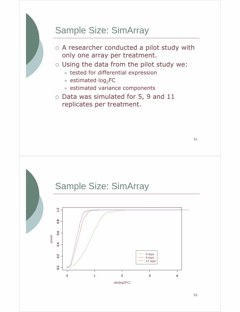
Sample Size: SimArray

� A researcher conducted a pilot study with only one array per treatment.

� Using the data from the pilot study we:

� tested for differential expression

� estimated log2FC

� estimated variance components

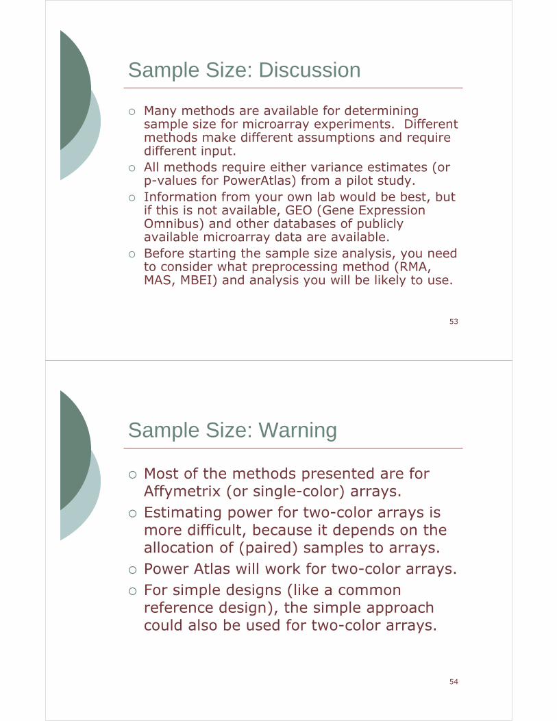
� Data was simulated for 5, 9 and 11 replicates per treatment.

52

Sample Size: SimArray

0 1 2 3 4

0.0

0.2

0.4

0.6

0.8

1.0

abs(log2FC)

pow

er

0 1 2 3 4

0.0

0.2

0.4

0.6

0.8

1.0

0 1 2 3 4

0.0

0.2

0.4

0.6

0.8

1.0

5 reps9 reps11 reps

53

Sample Size: Discussion

� Many methods are available for determining sample size for microarray experiments. Different methods make different assumptions and require different input.

� All methods require either variance estimates (or p-values for PowerAtlas) from a pilot study.

� Information from your own lab would be best, but if this is not available, GEO (Gene Expression Omnibus) and other databases of publicly available microarray data are available.

� Before starting the sample size analysis, you need to consider what preprocessing method (RMA, MAS, MBEI) and analysis you will be likely to use.

54

Sample Size: Warning

� Most of the methods presented are for Affymetrix (or single-color) arrays.

� Estimating power for two-color arrays is more difficult, because it depends on the allocation of (paired) samples to arrays.

� Power Atlas will work for two-color arrays.

� For simple designs (like a common reference design), the simple approach could also be used for two-color arrays.

55

5. Design for two-color Arrays

� Special consideration needs to be given for the design of experiments involving spotted arrays because 2 samples (one dyed “red” and one dyed “green”) are hybridized to a single array.

� Thought needs to be given to which samples are labeled with which “dye” and which are to be hybridized together on the same array.

56

Design for two-color arrays

“The ability to make direct comparisons between two samples on the same microarray slide is a unique and powerful feature of the two-color microarray system…However, it is often impractical to make all possible pairwise comparison among the samples because of cost or limitations in the amount of sample.”

Gary Churchill

57

Design for two-color arrays

“Gene-expression levels in two target samples can be compared only if there is a ‘path’ (that is, sequence of hybridizations) that joins the corresponding two vertices (mRNA samples). The precision of the estimates of relative expression, then, depends on the number of paths that join the two vertices, and is inversely related to the length of these paths.”

Y.H.Yang and T. Speed

58

Dye Swapping

� Before we talk about designs, we need to explain dye swapping.

� “Certain genes exhibit a dye bias- a tendency to bind more efficiently to one of the dyes” Dobbin et al. (2002)

� Dye swapping can be used to correct for the dye effect.

59

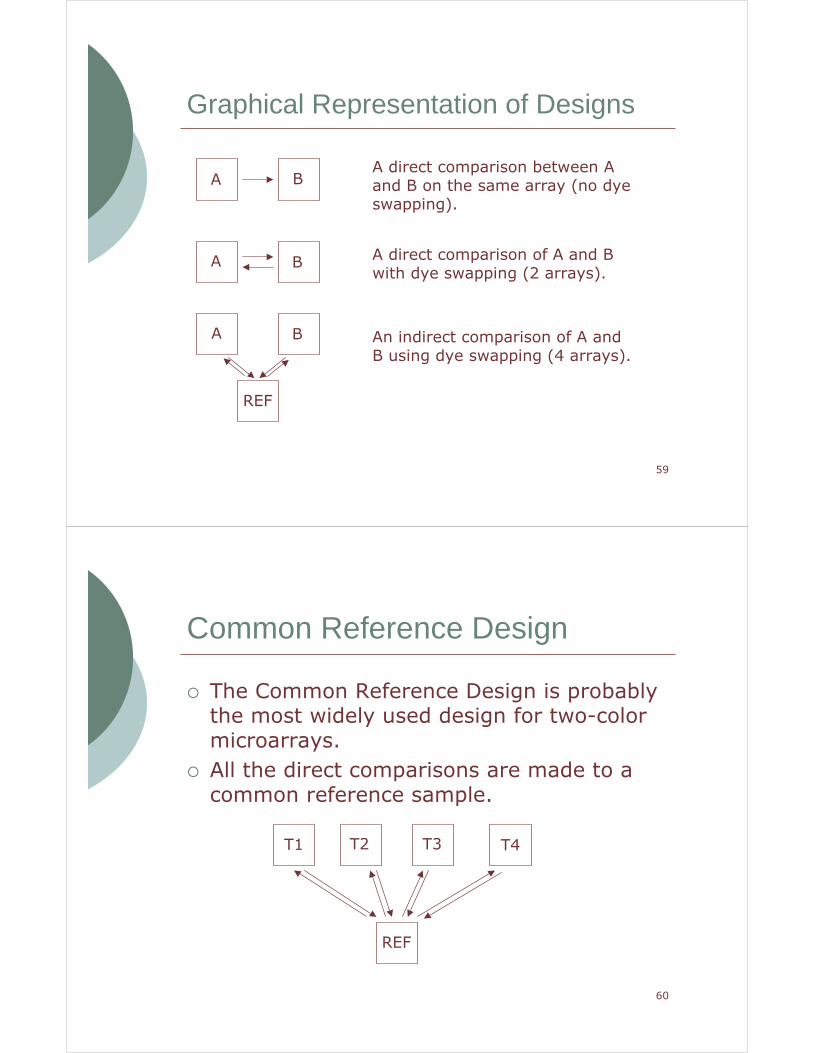
Graphical Representation of Designs

A B

A B

A B

REF

A direct comparison between A and B on the same array (no dye swapping).

A direct comparison of A and B with dye swapping (2 arrays).

An indirect comparison of A and B using dye swapping (4 arrays).

60

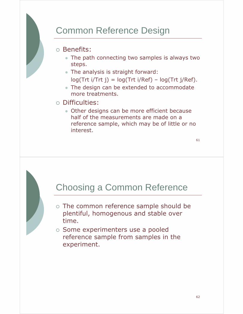
Common Reference Design

� The Common Reference Design is probably the most widely used design for two-color microarrays.

� All the direct comparisons are made to a common reference sample.

REF

T1 T2 T3 T4

61

Common Reference Design

� Benefits:

� The path connecting two samples is always two steps.

� The analysis is straight forward:

log(Trt i/Trt j) = log(Trt i/Ref) – log(Trt j/Ref).

� The design can be extended to accommodate more treatments.

� Difficulties:

� Other designs can be more efficient because half of the measurements are made on a reference sample, which may be of little or no interest.

62

Choosing a Common Reference

� The common reference sample should be plentiful, homogenous and stable over time.

� Some experimenters use a pooled reference sample from samples in the experiment.

63

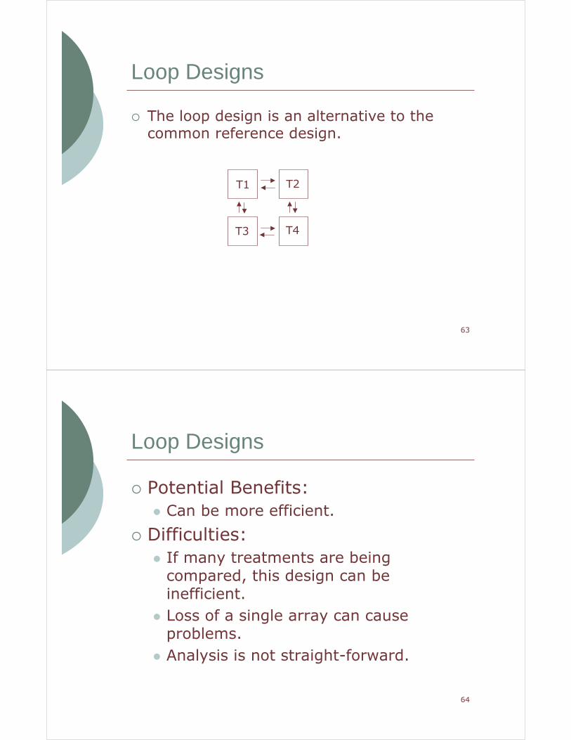
Loop Designs

� The loop design is an alternative to the common reference design.

T1 T2

T3 T4

64

Loop Designs

� Potential Benefits:

� Can be more efficient.

� Difficulties:

� If many treatments are being compared, this design can be inefficient.

� Loss of a single array can cause problems.

� Analysis is not straight-forward.

65

Designs for two color arrays

� Many other designs are possible.

� Biological replicates are still recommended, but technical replicates also tend to be used for spotted array experiments.

� Slides are usually printed in batches that can vary in quality. Even within a batch, the order and position on the printing device can effect results. Randomize!

66

6. Conclusions

� The design is driven by the goals of the experiment.

� Microarray experiments should use basic design principles: randomization, replication, and balance.

� Specialized approaches have been developed for determining sample size for microarray experiments.

� Results from microarray experiments are usually validated using RT-PCR.

67

References1. Getting Started:

� Han et al. (2004), Reproducibility, Sources of Variation, Pooling and Sample Size: Important Considerations for the Design of High-Density Oligonucleotide Array Experiments, Journal of Gerontology, 59A:306-315.

� Kuehl (2000), Design of Experiments: Statistical Principles of Research Design and Analysis.

� MAQC consortium (2006), The MicroArray Quality Control (MAQC) project shows inter- and intraplatform reproducibility of gene expression measurements, Nature Biotechnology, 24(9):1151-1161.

� Zakharkin et al. (2005), Sources of variation in Affymetrix miroarray experiments, BMC Bioinformatics, 6:214.

2. Pooling:� Kendziorski et al. (2005), On the utility of pooling biological

samples in microarray experiments, PNAS, 102(12):4252-4257.

68

References4. Sample Size

� Page et al. (2006), The PowerAtlas: a power and sample size atlas for microarray experimental design and research, BMC Bioinformatics, 7:84.

� Pavlidis et al. (2003), The effect of replication in gene expression microarray experiments, Bioinformatics, 19:1620-1627.

� Warnes and Liu, Sample Size Estimation for Microarray Experiments Using the ssize packagePackage and documentation available from: http://bioconductor.org/packages/1.9/bioc/html/ssize.html

� Zien et al. (2003), Microarrays: How Many Do You Need? Journal of Computational Biology, 10:653-667.

5. Two-Color Designs� Churchill (2002), Fundamentals of experimental design for

cDNA microarrays, Nature Genetics Supplement, 32:490-495.

� Dobbin et al. (2002), Statistical design of reverse dye microarrays, Bioinformatics, 19:803-810.

� Yang and Speed (2002), Design issues for cDNA microarray experiments, Nature Reviews Genetics, 3: 579-588.