Embed Size (px)
Citation preview

GUIDELINES
17M I C R O B I O L O G I C A L R I S K A S S E S S M E N T S E R I E S
Risk characterization of microbiological hazards in food
ISSN 1726-5274
For further information on the joint FAO/WHO activities on microbiological risk assessment, please contact:
Nutrition and Consumer Protection DivisionFood and Agriculture Organization of the United NationsViale delle Terme di Caracalla00153 Rome, Italy
Fax: +39 06 57054593E-mail: [email protected]
Web site: http://www.fao.org/ag/agn/agns
or
Department of Food Safety and Zoonoses World Health Organization20 Avenue AppiaCH-1211 Geneva 27Switzerland
Fax: +41 22 7914807E-mail: [email protected]
Web site: http//www.who.int/foodsafety
Cover design: Food and Agriculture Organization of the United Nations and the World Health Organization
Cover picture: © Dennis Kunkel Microscopy, Inc.
WORLD HEALTH ORGANIZATION
FOOD AND AGRICULTURE ORGANIZATION OF THE UNITED NATIONS
2009
Risk characterization of microbiological hazards in food
M I C R O B I O L O G I C A L R I S K A S S E S S M E N T S E R I E S
17
GUIDELINES
— iii —
Contents Acknowledgements vii
Contributors ix
Foreword xi
Abbreviations used in the text xii
1. INTRODUCTION 1 1.1 FAO/WHO Series of Guidelines on Microbiological Risk Assessment 1 1.2 FAO/WHO Guidelines for Risk Characterization 2
1.2.1 Risk characterization defined 2 1.2.2 Scope 2 1.2.3 Purpose 2 1.2.4 The evolution of microbiological risk assessment 2
1.3 Risk characterization in context 3 1.4 Reading these guidelines 3
2. PURPOSE OF MICROBIOLOGICAL FOOD SAFETY RISK ASSESSMENT 5 2.1 Properties of risk assessments 7
2.1.1 The need for the four components of risk assessment 7 2.1.2 Differentiating risk assessment and risk characterization 8
2.2 Risk characterization measures 8 2.3 Purposes of specific risk assessments 9
2.3.1 Estimating ‘unrestricted risk’ and ‘baseline risk’ 10 2.3.2 Comparing risk management strategies 11 2.3.3 Research-related study or model 13
2.4 Choosing what type of risk assessment to perform 14 2.5 Variability, randomness and uncertainty 16
2.5.1 Variability 16 2.5.2 Randomness 17 2.5.3 Uncertainty 17
2.6 Data gaps 18 2.6.1 The use of expert opinion 19
2.7 The role of best- and worst-case scenarios 20 2.8 Assessing the reliability of the results the risk assessment 21
3. QUALITATIVE RISK CHARACTERIZATION IN RISK ASSESSMENT 23 3.1 Introduction 23
3.1.1 The value and uses of qualitative risk assessment 24 3.1.2 Qualitative risk assessment in food safety 25
3.2 Characteristics of a qualitative risk assessment 26
— iv —
3.2.1 The complementary nature of qualitative and quantitative risk assessments 26 3.2.2 Subjective nature of textual conclusions in qualitative risk assessments 26 3.2.3 Limitations of qualitative risk characterization 27
3.3 Performing a qualitative risk characterization 29 3.3.1 Describing the risk pathway 29 3.3.2 Data requirements 29 3.3.3 Dealing with uncertainty and variability 29 3.3.4 Transparency in reaching conclusions 30
3.4 Examples of qualitative risk assessment 32 3.4.1 WHO faecal pollution and water quality 32 3.4.2 Australian Drinking Water Guidelines 33 3.4.3 EFSA BSE/TSE risk assessment of goat milk and milk-derived products 33 3.4.4 Geographical BSE cattle risk assessment 34
4. SEMI-QUANTITATIVE RISK CHARACTERIZATION 37 4.1 Introduction 37
4.1.1 Uses of semi-quantitative risk assessment 37 4.2 Characteristics of a semi-quantitative risk assessment 38 4.3 Performing a semi-quantitative risk assessment 40
4.3.1 Risks with several impact dimensions 41 4.3.2 Comparing risks and risk management strategies 42 4.3.3 Limitations of semi-quantitative risk assessment 43 4.3.4 Dealing with uncertainty and variability 45 4.3.5 Data requirements 45 4.3.6 Transparency in reaching conclusions 46
4.4 Examples of semi-quantitative risk assessment 46 4.4.1 New Zealand risk profile of Mycobacterium bovis in milk 46 4.4.2 Seafood safety using RiskRanger 48 4.4.3 Australia’s animal and animal product import-risk assessment methodology 50
5. QUANTITATIVE RISK CHARACTERIZATION 53 5.1 Introduction 53 5.2 Quantitative measures 53
5.2.1 Measure of probability 54 5.2.2 Measure of impact 54 5.2.3 Measures of risk 54 5.2.4 Matching dose-response endpoints to the risk measure 57 5.2.5 Accounting for subpopulations 58
5.3 Desirable properties of quantitative risk assessments 58 5.4 Variability, randomness and uncertainty 59
5.4.1 Modelling variability as randomness 59 5.4.2 Separation of variability and randomness from uncertainty 60
— v —
5.5 Integration of hazard characterization and exposure assessment 61 5.5.1 Units of dose in exposure assessment 61 5.5.2 Units of dose and response in dose-response assessment 62 5.5.3 Combining Exposure and Dose-response assessments 63 5.5.4 Dose-response model assumptions 64 5.5.5 Exposure expressed as prevalence 65 5.5.6 Epidemiological-based dose-response relationships 66 5.5.7 Integration of variability and uncertainty 67
5.6 Examples of quantitative risk analysis 74 5.6.1 FSIS E. coli comparative risk assessment for intact (non-tenderized) and non-
intact (tenderized) beef 74 5.6.2 FAO/WHO Listeria monocytogenes in ready-to-eat foods 74 5.6.3 Shiga-toxin-producing E. coli O157 in steak tartare patties 75 5.6.4 FAO/WHO risk assessment of Vibrio vulnificus in raw oysters. 76
6. QUALITY ASSURANCE 79 6.1 Data quality assurance 79
6.1.1 Data collection 79 6.1.2 Sorting and selecting data sources 82
6.2 Progression and weight of evidence 82 6.3 Sensitivity analysis 83
6.3.1 Sensitivity analysis in qualitative risk assessment 84 6.3.2 Sensitivity analysis in quantitative risk assessment 84
6.4 Uncertainty analysis 86 6.5 Model verification 88 6.6 Model anchoring 87 6.7 Model validation 87 6.8 Comparison with epidemiological data 88 6.9 Extrapolation and robustness 89 6.10 Credibility of the risk assessment 90
6.10.1 Risk assessment documentation 90 6.10.2 Peer review 91
7. LINKING RISK ASSESSMENT AND ECONOMIC ANALYSIS 93
7.1 Introduction 93 7.2 Economic valuation issues 94
7.2.1 Valuation of health outcomes 94 7.2.2 Valuation of non-health outcomes 96
7.3 Integrating economics into risk assessments to aid decision-making 97
7.3.1 Cost–benefit analysis 98 7.3.2 Cost effectiveness analysis 98
— vi —
7.3.3 Risk–cost trade-off curves 99 7.3.4 Uncertainty in economic analysis 99
8. RISK COMMUNICATION ASPECTS OF RISK CHARACTERIZATION 101 8.1 Introduction 101
8.1.1 Information to share with stakeholders 102 8.1.2 Major scientific issues in risk communication 102
8.2 Interaction between risk managers and risk assessors 102 8.2.1 Planning and commissioning an MRA 103 8.2.2 During the MRA 103
8.3 After the completion of the MRA 104 8.4 Development of risk communication strategies 105 8.5 Public review 108
REFERENCES CITED IN THE TEXT 109
APPENDIX 1 115

— vii —
Acknowledgements
The Food and Agriculture Organization of the United Nations (FAO) and the World Health Organization (WHO) would like to express their appreciation to all those who contributed to the preparation of these guidelines through the provision of their time and expertise, and relevant information and experience. Special appreciation is extended to the participants at the workshops that were held in both Denmark and Switzerland and for the time and effort that they freely dedicated before, during and after these workshops to the elaboration of these guidelines. Many people provided their time and expertise by reviewing the guidelines and providing their comments and all of these are listed in the following pages. Special appreciation is also extended to Dr Tom Ross and Dr Don Schaffner for the additional assistance they provided in reviewing the comments received from the peer review process and revising the guidelines as required.
The development of the guidelines was by the Secretariat of the Joint FAO/WHO Expert Meetings on Microbiological Risk Assessment (JEMRA). This included Sarah Cahill, Maria de Lourdes Costarrica and Jean Louis Jouve (up to 2004) in FAO, and Peter Karim Ben Embarek, Hajime Toyofuku (up to 2004) and Jocelyne Rocourt (up to 2004) in WHO. Publication of the guidelines was coordinated by Sarah Cahill. Final editing for language, style and preparation for publication was by Thorgeir Lawrence.
The work was supported and funded by the FAO Nutrition and Consumer Protection Division and the WHO Department of Food Safety and Zoonoses.
— ix —
Contributors
PARTICIPANTS AT THE DANISH WORKSHOP
John Bowers Food and Drug Administration, United States of America
Aamir Fazil Public Health Agency of Canada, Canada
Bjarke Bak Christensen Danish Veterinary and Food Administration, Denmark
Christopher Frey North Carolina State University, United States of America
Arie Havelaar National Institute of Public Health and the Environment, the Netherlands
Louise Kelly University of Strathclyde, United Kingdom
George Nasinyama Makerere University, Uganda
Maarten Nauta National Institute of Public Health and the Environment, the Netherlands
Niels Ladefoged Nielson Danish Veterinary and Food Administration, Denmark
Birgit Norrung Danish Veterinary and Food Administration, Denmark
Greg Paoli Decisionalysis Risk Consultants Inc., Canada
Mark Powell United States Department of Agriculture, United States of America
Tanya Roberts United States Department of Agriculture, United States of America
Don Schaffner Rutgers University, United States of America
Helle Sommer Danish Veterinary and Food Administration, Denmark
David Vose Vose Consulting, France
Danilo Lo Fo Wong Danish Veterinary Institute, Denmark
Marion Wooldridge Veterinary Laboratories Agency (Weybridge), United Kingdom
Charles Yoe College of Notre Dame of Maryland, United States of America

— x —
PARTICIPANTS AT THE SWISS WORKSHOP Robert Buchanan Food and Drug Administration, United States of America
Arie Havelaar National Institute of Public Health and the Environment, the Netherlands
Greg Paoli Decisionalysis Risk Consultants Inc., Canada
Don Schaffner Rutgers University, United States of America
David Vose Vose Consulting, France
Marion Wooldridge Veterinary Laboratories Agency (Weybridge), United Kingdom
PEER REVIEWERS Wayne Anderson Food Safety Authority of Ireland, Ireland
Linda Calvin United States Department of Agriculture, United States of America
Sherrie Dennis Food and Drug Administration, United States of America
Christopher Frey North Carolina State University, United States of America
Charles Haas Drexel University, United States of America
William Hallman Rutgers University, United States of America
Linda Harris University of California Davis, United States of America
LeeAnn Jaykus North Carolina State University, United States of America
Fumiko Kasuga National Institute of Infectious Diseases, Japan
Rob Lake Environmental Science and Research, New Zealand
Anna Lammerding Public Health Agency of Canada, Canada
Régis Pouillot Institut Pasteur, Cameroon
Mark Powell United States Department of Agriculture, United States of America
Moez Sanna National Veterinary School of Alfort, France
Richard Whiting Food and Drug Administration, United States of America
Marion Wooldridge Veterinary Laboratories Agency (Weybridge), United Kingdom

— xi —
Foreword
Members of the Food and Agriculture Organization of the United Nations (FAO) and of the World Health Organization (WHO) have expressed concern regarding the level of safety of food at both national and international level. Increasing foodborne disease incidence over recent decades seems, in many countries, to be related to an increase in disease caused by micro-organisms in food. This concern has been voiced in meetings of the Governing Bodies of both Organizations and in the Codex Alimentarius Commission. It is not easy to decide whether the suggested increase is real or an artefact of changes in other areas, such as improved disease surveillance or better detection methods for microorganisms in patients or foods. However, the important issue is whether new tools or revised and improved actions can contribute to our ability to lower the disease burden and provide safer food. Fortunately, new tools that can facilitate actions seem to be on their way.
Over the past decade, risk analysis—a process consisting of risk assessment, risk management and risk communication—has emerged as a structured model for improving our food control systems, with the objectives of producing safer food, reducing the number of food-borne illnesses and facilitating domestic and international trade in food. Furthermore, we are moving towards a more holistic approach to food safety, where the entire food chain needs to be considered in efforts to produce safer food.
As with any model, tools are needed for the implementation of the risk analysis paradigm. Risk assessment is the science-based component of risk analysis. Science today provides us with in-depth information on life in the world we live in. It has allowed us to accumulate a wealth of knowledge on microscopic organisms, their growth, survival and death, even their genetic make-up. It has given us an understanding of food production, processing and preservation, and of the link between the microscopic and the macroscopic world, and how we can benefit as well as suffer from these microorganisms. Risk assessment provides us with a framework for organizing these data and information and gaining a better understanding of the interaction between microorganisms, foods and human illness. It provides us with the ability to estimate the risk to human health from specific microorganisms in foods and gives us a tool with which we can compare and evaluate different scenarios, as well as identify the types of data necessary for estimating and optimizing mitigating interventions.
Microbiological risk assessment (MRA) can be considered as a tool that can be used in the management of the risks posed by foodborne pathogens, including the elaboration of standards for food in international trade. However, undertaking an MRA, particularly quantitative MRA, is recognized as a resource-intensive task requiring a multidisciplinary approach. Nevertheless, foodborne illness is one of the most widespread public health problems, creating social and economic burdens as well as human suffering., it is a concern that all countries need to address. As risk assessment can also be used to justify the introduction of more stringent standards for imported foods, a knowledge of MRA is important for trade purposes, and there is a need to provide countries with the tools for understanding and, if possible, undertaking MRA. This need, combined with that of the Codex Alimentarius for risk-based scientific advice, led FAO and WHO to undertake a programme of activities on MRA at international level.
The Nutrition and Consumer Protection Division (FAO) and the Department of Food Safety and Zoonoses (WHO) are the lead units responsible for this initiative. The two groups have worked together to develop MRA at international level for application at both national and international level. This work has been greatly facilitated by the contribution of people from

— xii —
around the world with expertise in microbiology, mathematical modelling, epidemiology and food technology, to name but a few.
This Microbiological Risk Assessment series provides a range of data and information to those who need to understand or undertake MRA. It comprises risk assessments of particular pathogen–commodity combinations, interpretative summaries of the risk assessments, guidelines for undertaking and using risk assessment, and reports addressing other pertinent aspects of MRA.
We hope that this series will provide a greater insight into MRA, how it is undertaken and how it can be used. We strongly believe that this is an area that should be developed in the international sphere, and the work to date clearly indicates that an international approach and early agreement in this area will strengthen the future potential for use of this tool in all parts of the world, as well as in international standard setting. We would welcome comments and feedback on any of the documents within this series so that we can endeavour to provide member countries, the Codex Alimentarius and other users of this material with the information they need to use risk-based tools, with the ultimate objective of ensuring that safe food is available for all consumers.
Ezzeddine Boutrif Jørgen Schlundt
Nutrition and Consumer Protection Division Department of Food Safety and Zoonoses
FAO WHO

— xiii —
Abbreviations used in the text
ALOP Appropriate Level of Protection
ANOVA Analysis of variance
BSE Bovine Spongiform Encephalopathy
EC European Commission
CAC Codex Alimentarius Commission
CCFH Codex Committee on Food Hygiene
CFU Colony-forming units
COI Cost-of-illness
DALY Disability-adjusted life years
EFSA European Food Safety Authority
FSIS [USDA] Food Safety and Inspection Service
GBR Geographical BSE-Risk
MRA Microbiological Risk Assessment
NACMCF [USDA/FSIS] National Advisory Committee on Microbiological Criteria for Foods
NHMRC National Health and Medical Research Council [Australia]
P-I probability-impact
QALY Quality adjusted life years
SPS [WTO Agreement on the Application of] Sanitary and Phytosanitary [Measures]
STEC Shiga-toxin-producing Escherichia coli
TSE Transmissible Spongiform Encephalopathy
USDA United States Department of Agriculture
VOI Value of information [analysis]
WTO World Trade Organization
WTP Willingness-to-pay

1. Introduction
1.1 FAO/WHO Series of Guidelines on Microbiological Risk Assessment
Risk assessment of microbiological hazards in foods (Microbiological Risk Assessment – MRA) has been identified as a priority area of work by the Codex Alimentarius Commission (CAC). Following the work of the Codex Committee on Food Hygiene (CCFH), CAC adopted Principles and Guidelines for the Conduct of Microbiological Risk Assessment (CAC/GL-30 (1999) – CAC, 1999). Subsequently, at its 32nd session, the CCFH identified a number of areas in which it required expert risk assessment advice. At the international level it should also be noted that the World Trade Organization (WTO) Agreement on the Application of Sanitary and Phytosanitary Measures (WTO, no date) requires members to ensure that their measures are based on an assessment of the risks, as appropriate to the circumstances, taking into account the risk assessment techniques developed by the relevant international organizations.
In response therefore to the needs of their member countries and Codex, FAO and WHO launched a programme of work with the objective of providing expert advice on risk assessment of microbiological hazards in foods. The purpose of this work is to provide an overview of the available relevant information as well as the risk assessments that have already been undertaken, and from these to develop risk-based scientific advice to address the needs of Codex and to develop risk assessment tools for use by member countries.
FAO and WHO also undertook development of guideline documents for the hazard characterization, exposure assessment, and risk characterization steps of risk assessment, the last-named being the subject of this volume. Details of other documents in the series and how they may be obtained are provided on the inside covers of this document. The need for such guidelines was highlighted in the work being undertaken by FAO and WHO on risk assessment of specific pathogen–commodity combinations and it is recognized that reliable and consistent estimates of risk in the risk characterization step are critical to risk assessment.
The FAO/WHO series of guidelines is intended to provide practical guidance and a structured framework for carrying out each of the four building blocks of a microbiological risk assessment (hazard identification, hazard characterization, exposure assessment, risk characterization), whether as part of a full risk assessment, as an accompaniment of other evaluations, or as a stand-alone process.
The primary audience for these MRA guidelines is the global community of scientists and risk assessors, both experienced and inexperienced in risk assessment, and the risk managers they serve.
The MRA guidelines are not intended to be prescriptive, nor do they identify pre-selected compelling options. On some issues, an approach is advocated based on a consensus view of experts to provide guidance on the current science in risk assessment. On other issues, the available options are compared and the decision on the approach appropriate to the situation is left to the analyst. In both of these situations, transparency requires that the approach and the supporting rationale be documented.

2 Introduction
1.2 FAO/WHO Guidelines for Risk Characterization
1.2.1 Risk characterization defined
Risk Characterization, as an element of MRA, was defined by CAC as:
“the qualitative and/or quantitative estimation, including attendant uncertainties, of the probability of occurrence and severity of known or potential adverse health effects in a given population based on hazard identification, hazard characterization and exposure assessment.”
It is in the risk characterization step that the results of the risk assessment are presented. These results are provided in the form of risk estimates and risk descriptions that provide answers to the questions risk managers pose to risk assessors. These answers, in turn provide the best available science-based evidence to be used by risk managers to assist them in managing food safety.
1.2.2 Scope
These guidelines address risk characterization and related issues in MRA. They provide descriptive guidance on how to conduct risk characterizations in various contexts, and utilizing a variety of tools and techniques. They have been developed in recognition of the fact that reliable estimation of risk is critical to the overall risk assessment.
1.2.3 Purpose
Although these guidelines may be prospective at times, anticipating where best practice may next lead, they are not intended to be considered prescriptive guidelines. Instead, this document is intended to provide practical guidelines on a structured framework for carrying out risk characterization of microbiological hazards in foods. As with other documents in the MRA series, the primary audience for these risk characterization guidelines is the global community of scientists and risk assessors, both experienced and inexperienced in risk assessment, and the risk managers they serve.
The overarching objectives of these guidelines are to help this audience to:
• identify the key issues and features of a risk characterization;
• recognize the properties of a best practice risk characterization;
• avoid some common pitfalls of risk characterization;
• recognize and understand assumptions that may be implicit in the choice of specific risk characterization measures; and
• prepare risk characterizations that are responsive to the needs of risk managers.
1.2.4 The evolution of microbiological risk assessment
Microbiological risk assessment of water has been undertaken since the early 1990s, and for foods since the mid-1990s, after the earlier development of nuclear and toxicological human health risk assessments. There has been just a decade of development of techniques for assessing microbiological risk, and for aligning the scientific disciplines that contribute data to risk assessment. These guidelines therefore represent the best practice at the time of their preparation. It is hoped that these guidelines and others produced in this series will help stimulate further developments and disseminate the current knowledge.

Risk characterization of microbiological hazards in food 3
1.3 Risk characterization in context
Risk characterization is the final step in the risk assessment component of risk analysis. Risk analysis comprises three elements: risk management, risk assessment and risk communication. Risk assessment is initiated by risk managers who develop risk assessment policy and give the risk assessment its direction by establishing the specific risk assessment goals and by posing specific questions to be answered by the risk assessment. The questions posed by managers are usually revised and refined in an iterative process of discovery, discernment and negotiation with risk assessors. Once answered, the risk managers have the science-based information they need to support their decision-making process with the science-based information they need to support their decision-making process.
Risk characterization is the risk assessment step in which most of the risk managers’ questions are addressed. While ‘risk characterization’ is the process, the result of the process is the ‘risk estimate’. The risk characterization can often include one or more estimates of risk, risk descriptions, and evaluations of risk management options that may include economic and other evaluations in addition to estimates of changes in risk attributable to the management options. The risk characterization should also address quality assurance of the overall risk assessment, as discussed in Chapter 6.
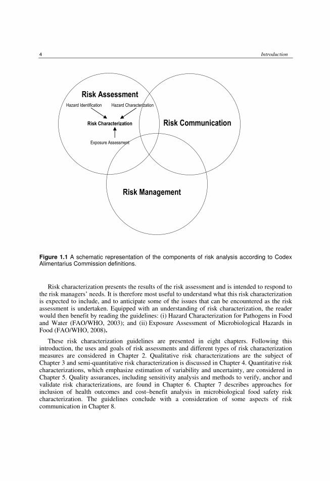
Many of the recent quantitative microbiological risk assessments use the Codex risk assessment framework (Figure 1.1). This entails a risk characterization that integrates relevant knowledge from the other three risk assessment steps—hazard identification, exposure assessment and hazard characterization—to obtain a risk estimate.
Although this is a common context for undertaking risk characterization, it is by no means the only context. In actual practice an assessment of the risk may include some or all of these steps. The scientific analyses comprising any one of these steps may be sufficient on their own for decision-making. For example, in Denmark, the number of human cases of salmonellosis attributed to different animal sources is estimated without a precise exposure assessment and without using a dose-response model (Hald et al., 2004). This could be done since serotypes and phagetypes are, to some extent, specific to the food source, i.e. epidemiological information indicating the type of Salmonellae causing human infection could be used to estimate the proportion of human cases due to each food type providing, in effect, a risk ranking of the various food sources.
Risk characterization, as used in these guidelines, cannot be represented by any one model or description. Commonly used approaches to risk characterization are described in the chapters that follow.
1.4 Reading these guidelines
FAO and WHO have produced a series of documents to support the conduct of microbiological risk assessments. Ideally, the risk assessor would begin with the Report of a Joint FAO/WHO Consultation entitled Principles and guidelines for incorporating microbiological risk assessment in the development of food safety standards, guidelines and related texts (FAO/WHO, 2002). That report appropriately establishes the purpose of risk assessment as meeting the needs of risk managers. With that report as background the reader would ideally read these guidelines for risk characterization next.
4 Introduction
Figure 1.1 A schematic representation of the components of risk analysis according to Codex Alimentarius Commission definitions.
Risk characterization presents the results of the risk assessment and is intended to respond to the risk managers’ needs. It is therefore most useful to understand what this risk characterization is expected to include, and to anticipate some of the issues that can be encountered as the risk assessment is undertaken. Equipped with an understanding of risk characterization, the reader would then benefit by reading the guidelines: (i) Hazard Characterization for Pathogens in Food and Water (FAO/WHO, 2003); and (ii) Exposure Assessment of Microbiological Hazards in Food (FAO/WHO, 2008).
These risk characterization guidelines are presented in eight chapters. Following this introduction, the uses and goals of risk assessments and different types of risk characterization measures are considered in Chapter 2. Qualitative risk characterizations are the subject of Chapter 3 and semi-quantitative risk characterization is discussed in Chapter 4. Quantitative risk characterizations, which emphasize estimation of variability and uncertainty, are considered in Chapter 5. Quality assurances, including sensitivity analysis and methods to verify, anchor and validate risk characterizations, are found in Chapter 6. Chapter 7 describes approaches for inclusion of health outcomes and cost–benefit analysis in microbiological food safety risk characterization. The guidelines conclude with a consideration of some aspects of risk communication in Chapter 8.
�����������
������������� ��
������������� ������������������������������������������������������
�
���������� ����� ���
����� ����� � �����

2. Purpose of microbiological food safety risk assessment
The purpose of MRA in the Codex framework is, at its most basic, “a systematic analytical approach intended to support the understanding and management of microbiological risk issues” (Fazil et al., 2005). In microbiological food safety, the outcomes of interest are usually the incidence of one or more types of human health effect attributable to a specific food, pathogen, process, region, distribution pathway or some combination. Those health effects include diarrhoeal illnesses, hospitalizations and deaths. In other microbiological risk assessments, other impacts, e.g. social, environmental and economic, might be considered as well.
Risk managers initially define the intended use of a risk assessment in their “preliminary risk management activities’ (see FAO/WHO, 2002). They can then be expected to interact with risk assessors to refine the specific questions to be answered, or scope, focus or outputs of the risk assessment in an iterative fashion, possibly throughout the conduct of the risk assessment. Risk managers are expected to ask risk assessors to answer a specific set of questions, which, when answered, provide the managers with the information and analysis they need to support their food safety decision process.
The statement of purpose for a risk assessment should be clear and should guide the form of the risk assessment output such as number of cases of illness per year attributable to the product or pathogen, ranking of risk from one food compared with others, or expected reduction in risk if various interventions are implemented. If the risk assessment aims to find the best option to reduce a risk, then the statement of purpose should also identify all potential risk management interventions to be considered in the risk assessment. The questions and the statement of purpose will, to a great extent, guide the choice of the approach to be taken to characterize the risk. The data and knowledge collected in a specific risk assessment can be combined and analysed in different ways to answer a number of different risk management questions. Analogously, however, if the purpose of the risk assessment is not clear initially, inappropriate data and knowledge may be collected, or combined and analysed in ways that—while providing insight into some aspects of the risk—do not provide clear answers or insights to specific questions of the risk manager to assist in making a decision. Consequently, the purpose(s) of a specific risk assessment should be clearly defined and articulated to the risk assessors responsible for conducting the risk characterization prior to commencing the risk assessment so that the relevant data is gathered, synthesized and analysed in a way that provides answers to the risk manager’s questions
It is imperative to have some understanding of the likelihood of different outcomes under different scenarios, such as alternative intervention strategies, for a risk manager to be able to make rational choices between them. Without addressing the probability component of a risk, the risk manager is faced with comparing outcomes that are simply ‘possible’.
Risk assessment is a decision tool. Its purpose is not necessarily to further scientific knowledge, but to provide risk managers with a rational and objective picture of what is known, or believed to be known, at a particular point in time. Inevitably, a risk assessment will not have included all possible information about a risk issue because of limited access (for example, time constraints for the collection of data, or unwillingness of data owners to share information) or because the data simply does not exist, and in the process of performing a risk assessment one

6 Purpose of microbiological food safety risk assessment
usually learns which gaps in knowledge are more, and which are less, critical. Broad distribution of a draft risk assessment, in which the data gaps and assumptions are clearly pointed out, may, however, elicit new information.
Sometimes what is known at a particular time is insufficient for a risk manager to be comfortable in selecting an intervention strategy. If the risk manager’s bases and criteria for making a particular decision (i.e. the ‘decision rule’) are well defined, a risk assessment carried out based on current knowledge can often provide guidance as to what, and how much, information would make the choice of the correct decision more clear. Another benefit of the risk assessment methodology is that it provides a basis for rational discussion and evaluation of data and potential solutions to a problem. Thus, it acts to create consensus among stakeholders around risk management strategies or helps to identify where additional data are required.
All risk assessments should be critiqued within the context of the decision question, i.e. which risk management strategies the risk manager wishes to select between, and what data are available to help in the evaluation of those strategies. For example, in the case of bovine spongiform encephalopathy (BSE), sufficient animal health surveillance data may be available to quantitatively characterize BSE prevalence in a cattle population, but the dose-response relationship for vCJD (the human form of BSE) is likely to remain unknown for the foreseeable future. Therefore, it would clearly be nonsense to criticise a BSE risk assessment for failing to include a dose-response component where there are insufficient data available on which to base a dose-response relationship. The purpose of a risk assessment is to help the risk manager make a more informed choice and to make the rationale behind that choice clear to any stakeholders. Thus, in some situations, a very quick and simple risk assessment may be quite sufficient for a risk manager’s needs. For example, imagine the risk manager is considering some change that has no cost associated with it, and a crude analysis demonstrates that the risk under consideration would be 10-90% less likely to occur following implementation of the change, with no secondary risks. For the risk manager, this may be sufficient information to authorize making the change, despite the high level of uncertainty and despite not having determined what the base risk was in the first place. Of course, most risk issues are far more complicated, and require balancing the benefits (usually human health impact avoided) and costs (usually the commitment of available resources to carry out the strategy, as well as human health impacts from any secondary risks) of different intervention strategies.
There are two basic concepts concerning probability. The first is the apparently random nature of the world; the second is the level of uncertainty we have about how the real world is operating. Together, they limit our ability to predict the future and the consequences of decisions we make that may affect the future. Microbiological food safety risk assessment is most affected by uncertainty: uncertainty about what is really happening in the exposure pathways that lead humans to become infected or to ingest microbiological toxins, uncertainty about processes that lead from ingestion or infection to illness and that dictate the severity of the illness in different people, and uncertainty about the values of the parameters that would describe the processes of those pathways and processes. These are discussed in Section 2.5.3. Some of those uncertainties are readily quantified with statistical techniques where data are available, which gives the risk manager the most objective description of uncertainty. If, however, a risk assessment assumes a particular set of pathways and causal relationships that are incorrect, the assessment will be flawed.
Risk characterization of microbiological hazards in food 7
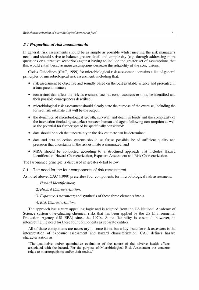
2.1 Properties of risk assessments
In general, risk assessments should be as simple as possible whilst meeting the risk manager’s needs and should strive to balance greater detail and complexity (e.g. through addressing more questions or alternative scenarios) against having to include the greater set of assumptions that this would entail because more assumptions decrease the reliability of the conclusions.
Codex Guidelines (CAC, 1999) for microbiological risk assessment contains a list of general principles of microbiological risk assessment, including that:
• risk assessment be objective and soundly based on the best available science and presented in a transparent manner;
• constraints that affect the risk assessment, such as cost, resources or time, be identified and their possible consequences described;
• microbiological risk assessment should clearly state the purpose of the exercise, including the form of risk estimate that will be the output;
• the dynamics of microbiological growth, survival, and death in foods and the complexity of the interaction (including sequelae) between human and agent following consumption as well as the potential for further spread be specifically considered;
• data should be such that uncertainty in the risk estimate can be determined;
• data and data collection systems should, as far as possible, be of sufficient quality and precision that uncertainty in the risk estimate is minimized; and
• MRA should be conducted according to a structured approach that includes Hazard Identification, Hazard Characterization, Exposure Assessment and Risk Characterization.
The last-named principle is discussed in greater detail below.
2.1.1 The need for the four components of risk assessment
As noted above, CAC (1999) prescribes four components for microbiological risk assessment:
1. Hazard Identification;
2. Hazard Characterization;
3. Exposure Assessment; and synthesis of these three elements into a
4. Risk Characterization.
The approach has a very appealing logic and is adapted from the US National Academy of Science system of evaluating chemical risks that has been applied by the US Environmental Protection Agency (US EPA) since the 1970s. Some flexibility is essential, however, in interpreting the need for these four components as separate entities.
All of these components are necessary in some form, but a key issue for risk assessors is the interpretation of exposure assessment and hazard characterization. CAC defines hazard characterization as
“The qualitative and/or quantitative evaluation of the nature of the adverse health effects associated with the hazard. For the purpose of Microbiological Risk Assessment the concerns relate to microorganisms and/or their toxins.”
8 Purpose of microbiological food safety risk assessment
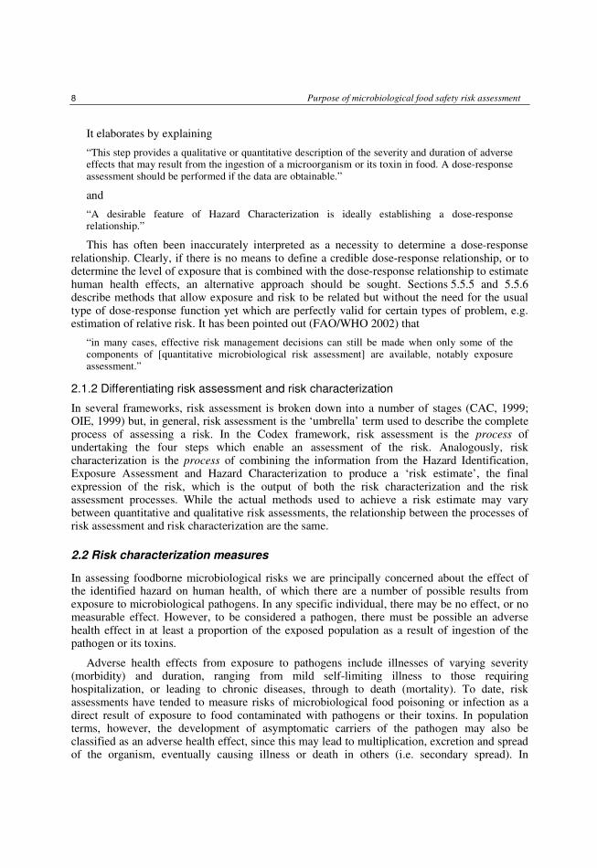
It elaborates by explaining
“This step provides a qualitative or quantitative description of the severity and duration of adverse effects that may result from the ingestion of a microorganism or its toxin in food. A dose-response assessment should be performed if the data are obtainable.”
and
“A desirable feature of Hazard Characterization is ideally establishing a dose-response relationship.”
This has often been inaccurately interpreted as a necessity to determine a dose-response relationship. Clearly, if there is no means to define a credible dose-response relationship, or to determine the level of exposure that is combined with the dose-response relationship to estimate human health effects, an alternative approach should be sought. Sections 5.5.5 and 5.5.6 describe methods that allow exposure and risk to be related but without the need for the usual type of dose-response function yet which are perfectly valid for certain types of problem, e.g. estimation of relative risk. It has been pointed out (FAO/WHO 2002) that
“in many cases, effective risk management decisions can still be made when only some of the components of [quantitative microbiological risk assessment] are available, notably exposure assessment.”
2.1.2 Differentiating risk assessment and risk characterization
In several frameworks, risk assessment is broken down into a number of stages (CAC, 1999; OIE, 1999) but, in general, risk assessment is the ‘umbrella’ term used to describe the complete process of assessing a risk. In the Codex framework, risk assessment is the process of undertaking the four steps which enable an assessment of the risk. Analogously, risk characterization is the process of combining the information from the Hazard Identification, Exposure Assessment and Hazard Characterization to produce a ‘risk estimate’, the final expression of the risk, which is the output of both the risk characterization and the risk assessment processes. While the actual methods used to achieve a risk estimate may vary between quantitative and qualitative risk assessments, the relationship between the processes of risk assessment and risk characterization are the same.
2.2 Risk characterization measures
In assessing foodborne microbiological risks we are principally concerned about the effect of the identified hazard on human health, of which there are a number of possible results from exposure to microbiological pathogens. In any specific individual, there may be no effect, or no measurable effect. However, to be considered a pathogen, there must be possible an adverse health effect in at least a proportion of the exposed population as a result of ingestion of the pathogen or its toxins.
Adverse health effects from exposure to pathogens include illnesses of varying severity (morbidity) and duration, ranging from mild self-limiting illness to those requiring hospitalization, or leading to chronic diseases, through to death (mortality). To date, risk assessments have tended to measure risks of microbiological food poisoning or infection as a direct result of exposure to food contaminated with pathogens or their toxins. In population terms, however, the development of asymptomatic carriers of the pathogen may also be classified as an adverse health effect, since this may lead to multiplication, excretion and spread of the organism, eventually causing illness or death in others (i.e. secondary spread). In
Risk characterization of microbiological hazards in food 9
addition, there may be adverse health effects of interest specifically at the population level, for example epidemics and pandemics.
Risks estimates can be made on an individual risk basis, e.g. risk of illness per serving, or on a population basis, e.g. ‘cases per annum’. While the Codex risk assessment framework focuses on severity and probability of disease, measures to compare disease severity are required. The burden of disease can be measured in terms of individual or national economic loss, if required, via probable numbers of days or years of working life lost, cost of treatment, etc., as discussed in Chapter 7 and Appendix 1. However, the measurement of loss of quality of life is harder to quantify, although various attempts have been made, resulting in the concept of equivalent life years lost through specific types of disability, pain or other reduced quality of life. This allows the comparison of one health state with another, and with mortality itself. Thus it is possible to quantify the adverse health effect of any occurrence in terms of life year equivalents lost, and estimate the risk of this from any specified source. Integrated health measures provide information to put diverse risks into context.
There are many potential adverse health effects that a risk manager might be interested in, in addition to those about which the affected individual is directly concerned. This, in turn means that there are many possible ways to measure and express the magnitude of the risk (sometimes called the ‘risk metric’) that might be selected as the required output from a risk assessment. The selection of the particular measure of risk to be used is therefore not necessarily straightforward, and must be discussed between the risk manager, the risk assessor, and other interested stakeholders. In addition, for quantitative modelling, the unit or units required must be defined whilst taking into account the practical aspects of modelling so that the outputs can be produced, and reported in those units.
2.3 Purposes of specific risk assessments
Various types of probability models and studies of risk issues have been labelled as ‘risk assessments’ (see Box 2.1). FAO/WHO, OIE and other guidelines advocate decision-making based on a risk assessment. Codex risk assessment guidelines and recommendations have legal significance in terms of what satisfies the food safety risk assessment requirements under the WTO Sanitary and Phytosanitary (SPS) Agreement. Thus, it is of both technical and legal importance to be able to determine whether a particular piece of work can be categorized as a risk assessment.
This section describes three categories of work that are often labelled ‘risk assessment’, and discusses when each type of study conforms to the necessary requirements. The three approaches are presented as examples, and other approaches to risk assessment are
Box 2.1 Examples of risk assessments developed for different purposes
• Danish Salmonella risk assessment apportioned human cases to different food animal sources.
• Health Canada E. coli O157 in ground beef, Dutch RIVM STEC O157 in steak tartare – all risk assessments for research and instruction.
• US FDA Listeria risk assessment for risk attribution to food categories.
• FAO/WHO Enterobacter sakazakii in powdered formula for evaluation of interventions
• USDA E. coli O157 and Salmonella Enteritidis risk assessments for intervention strategies.
• US FDA-CVM FQ-resistant Campylobacter risk assessment for human health impact estimation.

10 Purpose of microbiological food safety risk assessment
possible. No ‘correct’ approach can be recommended or specified: the choice of approach depends on the risk assessment question, the data and resources available, etc. The three categories considered are:
• Estimating an unrestricted or baseline risk.
• Comparing risk intervention strategies.
• Research-related study or model.
Risk assessment of the types described here can be used for purposes that might be considered ‘internal’ or ‘external’, depending, in part, on the range of stakeholders. The internal purposes might include activities such as setting priorities, allocating resources, and so on, within an organization, and the risk assessment not made public. External uses of risk assessment might be those that affect more stakeholders, such as those that result in changed regulations, or are undertaken as academic exercises, or as demonstrations of new or improved approaches to risk assessment. These are usually made public and are subject to peer review. Such assessments are frequently published in professional journals or made available on Web sites, or both.
2.3.1 Estimating ‘unrestricted risk’ and ‘baseline risk’
An ‘unrestricted risk’ estimate is the level of risk that would be present if there were no safeguards; and a ‘baseline risk’ estimate is the current, standard or reference status, i.e. the point against which the benefits and costs of various intervention strategies can be compared. The concept of unrestricted risk has been most widely used in import-risk analysis, in which it has more obvious utility.
A common and practical starting point for a risk assessment is to estimate the existing level of risk, i.e. the level of food safety risk posed without any changes to the current system. This risk estimate is most frequently used as the baseline risk against which intervention strategies can be valued, if desired. This baseline risk may, for example, have utility in determining an Appropriate Level of Protection (ALOP). Using the current risk as a baseline has a number of advantages, among them being that it is the easiest to estimate the effect of changes by estimating the magnitude of the risk after the changed conditions relative to the existing level of risk, i.e. it may obviate the need to explicitly quantify the risk level under either scenario. This approach implicitly accepts the starting point of any risk management actions as being changes to the current system. For some purposes, a baseline other than the existing level of risk might be used as a point of comparison. For example, the baseline risk could be set as that which would exist under some preferred (e.g. least costly) risk management approach, and the risk under alternative approaches compared with that.
Estimation of an unrestricted risk, i.e. the level of risk that would be present if no deliberate actions were taken to control the risk, sometimes referred to as inherent risk, may have a role in determining the efficacy of existing microbiological food safety risk management approaches compared with entirely new systems. Over time, as knowledge of the causes of infectious diseases grew, many controls to minimize foodborne illness have been implemented at the level of both consumers and the industry. While it is difficult to imagine being able to realistically assess the risk level in a hypothetical world where all those controls were removed, the principle is valid and takes as its point of departure a ‘raw’ risk that has been identified, and now quantified, and for which there are many combinations of options to choose from to control the risk. It would, in principle, enable reassessment of what combination of controls (both those in place and new possible interventions) would give the most efficient protection. In practice, one

Risk characterization of microbiological hazards in food 11
can attempt to estimate a risk where some of the more obvious, and perhaps more costly, interventions currently in place are removed, and then re-evaluate how to address the risk. Using the current risk level as the point of comparison does not encourage one to review the many layers of risk reduction activities that are already present, and have evolved over time in the absence of monitoring to evaluate their efficacy and to improve their efficiency. For example, control measures introduced before good information existed about a problem might be expected to be highly conservative. With improved knowledge, better targeted approaches could possibly be devised to deliver the same health protection with fewer disadvantages to consumers or producers.
Estimating a baseline or unrestricted risk may not be for the immediate purpose of managing the risk so much as to measure or bound the severity of a food safety problem. Whilst in theory it may not be necessary to determine a baseline risk in order to evaluate intervention strategies, it is nonetheless almost always carried out in practice.
A closely related activity is risk attribution, which apportions an identified risk among competing causes. This might involve apportioning food risks among pathogens, apportioning the risk associated with a specific pathogen among different food groups, or among different types of behaviour, like eating at barbecues or in restaurants. Risk attribution of a specific pathogen from different food sources could be used to rank food sources by the risk they pose. This helps the managers to identify the most important food or food source to control in order to most efficiently and cost effectively control the disease.
2.3.2 Comparing risk management strategies
Risk assessment is commonly undertaken to help risk managers understand which, if any, intervention strategies can best serve the needs of food safety, or if current risk management actions are adequate. Ideally, agencies with responsibility for safety of foods would consider all possible risk management interventions along the food chain without regard to who has the authority to enact them, and this objective has led to the creation of integrated food safety authorities in many nations and regions. A farm-to-table model may be most appropriate for this purpose. In practice, however, the scope of the assessment may be limited to those sections of the food chain within the risk manager’s area of authority, but a more comprehensive risk assessment might identify relationships outside that area of authority that would motivate the risk manager to seek the new authority required to intervene effectively or to request others with authority to take appropriate actions. For some risk questions, analysis of epidemiological data or a model of part of the food chain may be adequate. As discussed elsewhere, some risk assessments may be undertaken to ascertain whether existing food safety regulations and existing intervention strategies are adequate, or most appropriate, and if they require review.
Evaluations of putative risk management actions are often based on comparisons of a baseline risk estimate with a forecast risk that could result from pursuing various alternative strategies. These are sometimes called ‘what-if’ scenarios (see Box 2.2). One includes a future with no new intervention, the other a future with a new intervention. Initially, a baseline model (i.e. the ‘without intervention’ scenario) is constructed and run to give a baseline estimate of risk. Then selected model parameters are changed to determine the probable effect of the putative intervention(s) (see Box 2.3 for examples of interventions). The differences between the two risk estimates offer strong indications of the public health benefits of the proposed intervention(s) and, if possible, could also indicate the costs required to attain them. Combinations of interventions can be investigated in a similar fashion, to determine their joint effect, in an effort to find the optimal strategy
12 Purpose of microbiological food safety risk assessment
In some cases it is possible to estimate the change in risk without producing an estimate of the baseline risk, but caution must be used in these cases. For example, a risk assessment might determine that it is technically feasible to reduce a particular risk one-hundred-fold, but if this risk was negligible at the start, then reducing it one-hundred-fold may not be a worthwhile course of action.
The ‘proximity’ of a risk is commonly considered in risk analysis applied to management of large construction projects, and in certain circumstances will also be an important factor in food safety risk assessment if unplanned or uncontrolled factors could be expected to change the risk over time, e.g. the increase in average age of populations in many nations is expected to increase overall population susceptibility to many disease, including foodborne diseases,
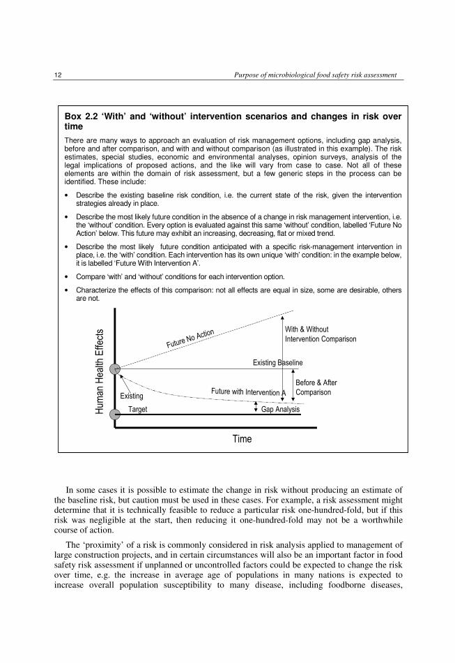
Box 2.2 ‘With’ and ‘without’ intervention scenarios and changes in risk over time There are many ways to approach an evaluation of risk management options, including gap analysis, before and after comparison, and with and without comparison (as illustrated in this example). The risk estimates, special studies, economic and environmental analyses, opinion surveys, analysis of the legal implications of proposed actions, and the like will vary from case to case. Not all of these elements are within the domain of risk assessment, but a few generic steps in the process can be identified. These include:
• Describe the existing baseline risk condition, i.e. the current state of the risk, given the intervention strategies already in place.
• Describe the most likely future condition in the absence of a change in risk management intervention, i.e. the ‘without’ condition. Every option is evaluated against this same ‘without’ condition, labelled ‘Future No Action’ below. This future may exhibit an increasing, decreasing, flat or mixed trend.
• Describe the most likely future condition anticipated with a specific risk-management intervention in place, i.e. the ‘with’ condition. Each intervention has its own unique ‘with’ condition: in the example below, it is labelled ‘Future With Intervention A’.
• Compare ‘with’ and ‘without’ conditions for each intervention option.
• Characterize the effects of this comparison: not all effects are equal in size, some are desirable, others are not.
����
�����
�����
�����
��� ������� �����
��� ����
�������!��������
�������"���������#���������������$������������ ��
%����$�%�����������#������������� ��
&����� '�������( �
&���

Risk characterization of microbiological hazards in food 13
leading to increased incidence. In other situations the risk may be seasonal, or arise only after natural disasters, or be linked to some specific event involving a very large gathering of people, etc. ‘Proximity’ describes the period or interval of time during which the risk might affect the stakeholders. A natural tendency is to focus on risks that are immediate when we may have a limited ability to manage them: assessing risks that could arise in the future might enable risk management steps to be implemented at a fraction of the cost of that for an emergency response when the risk has been realized.
The ‘proximity’ of a risk is commonly considered in risk analysis applied to management of large construction projects, and in certain circumstances will also be an important factor in food safety risk assessment if unplanned or uncontrolled factors could be expected to change the risk over time, e.g. the increase in average age of populations in many nations is expected to increase overall population susceptibility to many disease, including foodborne diseases, leading to increased incidence. In other situations the risk may be seasonal, or arise only after natural disasters, or be linked to some specific event involving a very large gathering of people, etc. ‘Proximity’ describes the period or interval of time during which the risk might affect the stakeholders. A natural tendency is to focus on risks that are immediate when we may have a limited ability to manage them: assessing risks that could arise in the future might enable risk management steps to be implemented at a fraction of the cost of that for an emergency response when the risk has been realized.
2.3.3 Research-related study or model
It has already been stated that risk assessment is a decision tool, not a scientific or research tool. Some research-based risk assessments have been produced with the intention of expanding our knowledge and tools for evaluating risks. They may be based on hypothetical or on genuine decisions questions, and evaluate the assessment results according to how they respond to those questions. However, they are not always initiated by a ‘risk manager’.
There are a number of large microbiological food safety models in existence that have been initiated as academic exercises. These models have helped advance the field of microbiological risk assessment by allowing us to see what techniques are necessary, developing new techniques, and stimulating research that can now be seen to have value within a risk assessment context. In some situations, those models have subsequently been used by risk managers to assist in risk management decisions. Such models have also made apparent the changes in collection and reporting methods for microbiological, epidemiological, production, dietary and other data that would make the data more useful for risk assessment.
In some instances risk managers are labouring in ignorance about the nature of a food safety problem. In this case, a risk assessment may be commissioned to simply expand the knowledge base.
Box 2.3 Examples of Microbiological Risk Management Interventions
• Vaccination of farm animals.
• HACCP and similar approaches during processing.
• Refrigeration and specification of ‘use by’ or ‘best before’ dates.
• Establishment of microbiological criteria.
• Use of ‘Hurdle Concept’ to limit pathogen growth.
• Product labelling for traceability.
• Consumer education, e.g. for ‘at-risk’ consumers.
14 Purpose of microbiological food safety risk assessment
Research is needed to do good risk assessment, but risk assessment is also a very useful aid in identifying where gaps in knowledge exist and thus where additional information is needed. A risk assessment may be undertaken specifically or incidentally to identify research needs, to establish research priorities, and to design commissioned studies.
Early experience with microbiological risk assessments has proven these assessments to be valuable in aiding our understanding of complex systems. The very process of systematically investigating a food chain has contributed to our ability to both appreciate and understand the complexity of the systems that make up the food chain.
2.4 Choosing what type of risk assessment to perform
Risk assessments methods span a continuum from qualitative through semi-quantitative to fully quantitative. All are valid approaches to food safety risk assessment, but the appropriateness of a particular method ultimately depends on the ability of the risk assessment to match the desirable characteristics listed in Section 2.1. Chapters 3 to 5 describe and provide examples from this continuum. While the chapter headings and examples might imply the existence of three strict categories of risk assessment methodology, the three terms are descriptions only and are used simply for convenience for organization of the document, and any risk assessment might include elements of any combination of these approaches. A benefit of risk assessment as a whole is that solutions to minimize risk often present themselves out of the formal process of considering risk, whether the risk assessment that has been conducted is qualitative, semi-quantitative or quantitative.
The importance of matching the type of risk assessment to its purpose has been emphasized previously. The USA National Advisory Committee on Microbiological Criteria for Foods noted (USNACMCF, 2004):
“Risk assessments can be quantitative or qualitative in nature, but should be adequate to facilitate the selection of risk management options. The decision to undertake a quantitative or qualitative risk assessment requires the consideration of multiple factors such as the availability and quality of data, the degree of consensus of scientific opinion and available resources.”
The Australian National Health and Medical Research Council note (NHMRC, 2004: 3–6) cautions that:
“Realistic expectations for hazard identification and risk assessment are important. Rarely will enough knowledge be available to complete a detailed quantitative risk assessment. ... A realistic perspective on the limitations of these predictions should be understood by staff and conveyed to the public.”
The decision on the appropriate balance of the continuum of methods from qualitative to quantitative will be based on a number of factors, including those considered below.
Consistency
A desire for consistency can work both for and against a decision to apply qualitative risk assessment. On the one hand, qualitative and semi-quantitative risk assessment can be made simple enough to be applied repeatedly across a range of risk issues, whereas quantitative risk assessment is more driven by the availability of data and may have to employ quite disparate methods to model different risks. Subjectivity can occur in quantitative risk assessments, e.g. in approaches to the selection and analysis of data, but the basis of these judgements can usually be documented in a way that enables others to replicate the results. Nonetheless, comparison of
Risk characterization of microbiological hazards in food 15
assumptions and data quality may be difficult. On the other hand, qualitative risk assessment is more prone to subjective judgements involved in converting data or experience into categories such as ‘high’, ‘intermediate’ and ‘low’ because it may be difficult to unambiguously define these terms, so repeatability of an analysis by others is less certain.
Expertise
Quantitative risk assessments typically require that at least part of the assessment team have rigorous mathematical training. If this resource is in limited supply, this may make qualitative risk assessment more appropriate, as long as the risk question is amenable to this approach. Note that, though qualitative risk assessments may not be demanding in terms of pure mathematical ability, they place a considerable burden of judgement on the analyst to combine evidence in an appropriate and logical manner, and the technical capability necessary to collate and interpret the current scientific knowledge is almost the same.
Theory or data limitations
Quantitative risk assessments tend to be better suited for situations where mathematical models are available to describe phenomena and where data are available to estimate the model parameters. If either the theory or data are lacking, then a more qualitative risk assessment is appropriate.
Breadth of application
When considering risks across a spectrum of hazards and pathways, there may be problems in applying quantitative risk assessment consistently across a diverse base of theory and evidence, such as comparing microbiological and chemical hazards in food. The methodologies and measurement approaches may not yet be able to provide commensurate risk measurements for decision-support where scope is broad.
Speed
Qualitative and semi-quantitative risk assessments generally require much less time to generate conclusions compared with quantitative risk assessment. This is particularly true when the protocols for qualitative and semi-quantitative risk assessments have been firmly established with clear guidance in the interpretation of evidence. There may be some exceptions where the process of qualitative risk assessment relies on a process of consultation (e.g. when relying heavily on structured expert elicitation) that requires considerable planning, briefing, and scheduling.
Transparency
The desire for transparency can favour all methods, depending on the type of transparency that is desired. Transparency, however, is not the same as ‘accessibility’. Transparency, in the sense that every piece of evidence and its exact impact on the assessment process is made explicit, is more easily achieved by quantitative risk assessment. However, accessibility, where a large audience of interested parties can understand the assessment process, may be better achieved through qualitative or semi-quantitative risk assessment. Quantitative microbiological risk assessment often involves specialized knowledge and a considerable time investment. As such, the analysis may only be accessible to specialists or those with the time and resources to engage
16 Purpose of microbiological food safety risk assessment
them. Strict transparency is of limited benefit where interested parties are not able, or find it excessively burdensome, to understand, scrutinize and contribute to the analysis and interpretation. Qualitative or semi-quantitative approaches may be easier to understand by a larger range of stakeholders, who will then be better able to contribute to the risk analysis process
Stage of analysis
Qualitative and quantitative risk assessment need not be mutually exclusive. Qualitative risk assessment is very useful in an initial phase of risk management to provide timely information regarding the approximate level of risk and to decide on the scope and level of resources to apply to quantitative risk assessment. As an example, qualitative risk assessment may be used to decide which exposure pathways (e.g. air, food, water; or raw versus ready-to-eat foods) will be the subject of a quantitative risk assessment.
Responsiveness
A major concern often expressed in regulatory situations is the lack of responsiveness of risk characterization measures or conclusions when faced with new evidence. Consider a situation where a risk assessment has been carried out with older data indicating that the prevalence of a pathogen is 10%. After the risk assessment is published, it is found that the prevalence has been reduced to 1%. In most quantitative risk assessments, there would be a clear impact of the reduced prevalence on the risk characterization. In some qualitative risk assessments, this impact may not be sufficiently clear. Qualitative risk assessments, particularly where the link between evidence and conclusion is ambiguous, may be considered to foster or support this lack of responsiveness. The unresponsiveness can generate mistrust and concern for the integrity of the risk assessment process.
2.5 Variability, randomness and uncertainty
Variability, randomness and uncertainty are frequently confused because all three can be described by distributions. However, they have distinct meanings, and a common understanding between the risk manager and risk assessor of these concepts can greatly help in the risk assessment process. These topics are also considered in Section 5.4, but in the context of quantitative risk assessment and mathematical modelling approaches.
2.5.1 Variability
Variability, also sometimes referred to as inter-individual variability, refers to real differences in values of some property of a ‘population’ over time or space of between individuals, whether the population refers to people, units of food, a species of foodborne pathogen etc. Examples of variable factors relevant to microbiological risk assessment include the storage temperatures of food products, seasonality of different food preparation methods (e.g. barbecuing), culinary practice, susceptibility to infection across subpopulations, consumption patterns across a region, differences in virulence between strains, and product handling processes across different producers.
In some cases, some of the variability in the population can be explained by observable individual attributes. For example, while the human population is heterogeneous; there may be discernable differences in risk between identifiable subpopulations because they are for some reason less frequently exposed, or less susceptible, to the hazard of interest. Or there could be

Risk characterization of microbiological hazards in food 17
three different methods of storing a food product, e.g. three different temperatures and corresponding humidity, leading to different potential for microbiological growth, and the fractions of the food item that are stored in each manner.
When there are discernable differences in risk due to known factors, ‘stratification’ of some type can be a practical method of addressing the population variability by recognizing those populations as discrete within the risk assessment. The properties of each subpopulation may still be described as a variable quantity, but with a different mean value and spread of values. There are many ways of stratifying a human population based on demographic, cultural, age and other variables, but foodborne pathogen risk stratifications are usually done in one of two ways. One is based on differences in exposure and the other is due to differences in susceptibility. These strata may also overlap. Within the population of interest, evidence should be sought of differences in susceptibility and of any likelihood of food-associated differential exposure patterns. If any differences found are likely to either significantly affect the risks or the potential safeguards, consideration should be given to stratifying the risk characterization based on these differences.
Variability is, in principle, described by a list of the different values that the variable takes. Often however, there are such a large number of values (for example, some characteristic about a human population, which will have millions of individuals) that it is more convenient to describe the variation using a frequency distribution.
2.5.2 Randomness
Randomness is due to the effect of chance inherent in the real world, and has also been described as aleatory uncertainty and stochastic variability.
There is debate about whether randomness actually exists, or simply reflects our imperfect knowledge of the real world, but for practical purposes the residual variation not explained by a model (i.e. a description embodying our understanding) is often treated as inherent randomness (Morgan and Henrion, 1990). An example of randomness in the context of MRA is given in Section 5.4.1, which also illustrates the interplay between variability, randomness and the use of stratification, as discussed above.
2.5.3 Uncertainty
Uncertainty is due to lack of knowledge regarding the true value of a quantity, and is also termed epistemic uncertainty, lack-of-knowledge uncertainty, or subjective uncertainty. It is often stated that variability and randomness are properties of the system being studied, whereas uncertainty is a property of the analyst. Different analysts, with different states of knowledge or access to different datasets or measurement techniques, will have different levels of uncertainty regarding the predictions that they make. An understanding of uncertainty is important because it provides insight into how lack of knowledge can influence decisions. When the range of uncertainty is large enough that there is ambiguity as to which decision alternative is preferred, then there may be value in collecting additional data or conducting additional research in order to reduce uncertainty.
Uncertainty is associated not only with the inputs to an assessment model, but also regarding the scenarios assumed for the assessment and the model itself. Sources of scenario uncertainty include potential misspecification of the harmful agents of concern, exposure pathways and vectors, exposed populations, and the spatial and temporal dimensions of the problem. Sources of model uncertainty include model structure, detail, resolution, validation or lack thereof, extrapolation, and boundaries of what is included and what is excluded from the model. Morgan
18 Purpose of microbiological food safety risk assessment
and Henrion (1990) and Cullen and Frey (1999) provide examples of sources of uncertainty in risk assessment, including the following:
• Random error. This is associated with imperfections in measurement techniques or with processes that are random or statistically independent of each other. Random measurement error leads to uncertainty that can be reduced by additional measurements, and is inversely related to precision. Precision refers to the agreement among repeated measurements of the same quantity.
• Systematic error. The mean value of a measured quantity may not converge to the "true" mean value because of biases in measurements and procedures. Such biases may arise from imprecise calibration, faulty reading of meters, and inaccuracies in the assumptions used to infer the actual quantity of interest from the observed readings of other quantities.
• Lack of empirical basis. Risk assessment often involves questions for which direct testing and observation is neither practical nor possible so that assumptions must be made based on available evidence. The validity of these assumptions cannot be assessed empirically. This type of uncertainty cannot be treated using conventional statistical techniques, because it requires predictions about something that has yet to occur or to be, tested, or measured. An example is the use of surrogate data when data are not available for the population of concern. Uncertainty about how well the surrogate data represents the population of concern can be characterized using expert judgements.
• Dependence and correlation. When there is more than one uncertain quantity, it may be possible that the uncertainties may be statistically or functionally dependent. Failure to properly model the dependence between the quantities can lead to uncertainty in the result, in terms of improper prediction of the variance of output variables.
• Disagreement. Where there are limited data or alternative theoretical bases for modelling a system, experts may disagree on the interpretation of data or on their estimates regarding the range and likelihood of outcomes for empirical quantities. In cases of expert disagreement, it is usually best to explore separately the implications of the judgements of different experts to determine whether substantially different conclusions about the problem result. If the conclusions are not significantly affected, then the results are said to be robust to the disagreements among the experts. If this is not the case, then one has to more carefully evaluate the sources of disagreement between the experts. In some cases, experts may not disagree about the body of knowledge. Thus, the differences in expert opinion may be reduced to clearly identified differences in inferences that the experts make from the data.
2.6 Data gaps
All risk assessments require data and knowledge (of processes, interactions, etc.), irrespective of whether they are qualitative or quantitative. Data (and knowledge) gaps influence the assessor’s confidence in the risk characterization and the robustness of the estimate. The form of a risk assessment is determined primarily by looking at what decision questions need to be answered. Then a search is done to see what data and knowledge are available that would help construct a logical risk-based argument (the risk assessment) that answers these questions. A balance is generally needed: taking a particular risk assessment approach may not be able to answer all questions, but may provide a better quality answer. Data may not be available to answer the question at all. Thus, defining the form of a risk assessment may require considerable dialogue between assessor and manager.
Risk characterization of microbiological hazards in food 19
This process will often lead to a better understanding of the value of other information that is not currently available. One can ask what else could be done if some specific data could be found. Depending on the time left until a decision has to be made, and on the resources available, the risk manager may consider it worth waiting, or expending the resources to acquire those data, and hopefully be able to make a more informed judgement as a result.
It is tempting to plan out the structure of a risk assessment that will answer all the risk managers’ questions, and then attempt to find the data required to ‘populate’ the risk assessment. However, in the food safety arena this may not be a practical approach. Food safety management is beset by a lack of data, so writing a wish list of all the data one would like will inevitably lead to disappointment. Other approaches, such as building simplified model-based reasoning to describe the system or process before considering the data availability, have been proposed as preliminary activities to aid in determining the form of the risk assessment. More complete discussion of data gaps can be found elsewhere (Fazil et al., 2005; FAO/WHO, 2008), but a brief list of reasons for such gaps includes:
• it has not previously been seen to be important to collect these data;
• data are too expensive to obtain;
• data are impossible to obtain given current technology;
• past data are no longer relevant;
• data from other regions are not considered relevant; or
• the data have been collected or reported, or both, in a fashion that does not match the risk assessment needs.
Data that has not previously been seen to be important often arises in contamination studies with infrequent positive data. Such data are not usually valuable for scientific journals; therefore researchers have less interest in conducting such studies. However, negative data are important for risk assessment, e.g. to estimate prevalence.
Using the risk assessment framework, it may be possible to determine which gaps have the most influence on being able to address the risk management questions. This identification process can be used to set priorities for future data collection and experimental research.
2.6.1 The use of expert opinion
It may be necessary to elicit expert estimates for parameter values in the pathway model where there is a critical lack of data, and where for pragmatic reasons it is essential to assess that risk in the relatively near future. Problems here include, for example, decisions on identification and selection of experts, the number of experts required, techniques for eliciting information, overcoming bias, etc., and methods are developing in this area (see, for example, Jenkinson, 2004).
When expert opinion is required, the problems and methods of selection, overcoming bias, etc., up to this point are likely to be similar for qualitative and quantitative risk assessments. Details on these methods are discussed elsewhere in the FAO/WHO guidelines (FAO/WHO 2003, 2008). It is accepted that ideally a ‘sufficient number’ of experts should be utilized. Techniques like the Delphi method (Linstone and Turoff, 1975), which aim to achieve consensus among a panel of experts, can help produce more reliable estimates from the available information. However, there are situations when there truly are very few, and on

20 Purpose of microbiological food safety risk assessment
occasions perhaps only one, expert in the specific topic worldwide. Sometimes there are no true experts. This leads to the use of inputs with very wide levels of uncertainty, whatever the risk assessment type, which is far from ideal but may on occasion be the only option in the short term.
In a quantitative risk assessment, it is necessary to convert expert opinion into a numerical input, and once again various methods exist and are being actively developed (see, for example, Gallagher et al
., 2002). Even in a qualitative risk assessment, these methods may also be used to convert expert opinion into numerical values for specific model steps, and this is, where time allows, the preferred method. As noted earlier, when used to describe approaches to risk assessment, the terms quantitative or qualitative do not refer to formally defined categories of risk assessment. An alternative and less sophisticated way of using expert opinion in qualitative risk assessments, however, may be to ask directly for an opinion on the probability of a specific step in narrative terms of, for example, high, low, negligible, etc. The meanings of these words will have the same subjectivity problems as has is discussed for qualitative risk assessments in general (see Chapter 3), and the reader’s evaluation of the results will need to be based on their evaluation of the experts selected. In principle, such a method should be only a temporary measure until improved data are available.
2.7 The role of best- and worst-case scenarios
As a filtering technique in risk assessment, e.g. as part of a risk profile, it may be useful to evaluate the best- or worst-case scenario to get a sense of ‘how good could it be’ or ‘how bad could it be’. The worst case scenario is usually used to filter out whether a risk or an exposure pathway is worth worrying about. No further analysis is necessary if the most pessimistic estimate shows the risk level to be below some threshold of interest (e.g. a negligible-risk level).
Conversely, a best-case scenario can be used as a preliminary filter of possible risk management options. The risk manager can discount any options for which the most optimistic estimate of the benefits the options could offer does not justify the cost of that option
Best- and worst-case scenarios operate somewhat like extreme ‘what-if’ scenarios. Where there is considerable but quantified uncertainty about a model parameter, a value is used that gives the required extreme. This will usually be an extreme value from the uncertainty distribution of the parameter, like its 1st or 99th percentile. However, when there is not a monotonic relationship between the parameter value and the risk estimate (i.e. that the magnitude of the risk estimate only increases/decreases as the parameter value increases/decreases or, conversely that the magnitude of the risk estimate only decreases/increases as the parameter value increases/decreases), the extreme estimate of risk may occur more towards the centre of the parameter’s uncertainty distribution.
Where there is uncertainty about exposure pathways and risk attribution, the extreme risk estimate is achieved by picking the most pessimistic (or optimistic) pathway: for example, ‘imagine that all salmonella came from chicken’.
Potential problems with worst-case analyses include that the analysis usually focuses on the consequences of the worst case, without the context of the probability of that worst-case scenario occurring, and that it is difficult to specify the conditions that might lead to the worst (or best) case: absolute extremes may be limited only by our imaginations. Conversely,
Risk characterization of microbiological hazards in food 21
wherever parameter values or exposure pathways are known with considerable certainty, they should be used to avoid exaggerating the extreme scenario beyond what is feasible.
Evaluating best- and worst-case scenarios can be considered as a risk assessment if the information about the extreme probability is credible and sufficient for the decision-maker.
2.8 Assessing the reliability of the results the risk assessment
Every risk assessment has some degree of uncertainty attached to its results. Complying with all the requirements of transparency, of describing model and parameter uncertainties, and all the explicit and implicit assumptions, does not necessarily communicate to risk managers the degree of confidence that the risk assessor has in the results of the risk assessment or limitations in its application. Thus, risk assessors must explain the level of confidence they feel should be attached to the risk assessment results. All assumptions should be acknowledged and made explicit in a manner that is meaningful to a non-mathematician. For example, it would be insufficient to say that ‘illnesses were assumed to follow a Poisson process’: a better explanation would be ‘illnesses were modelled as a Poisson process, which means that each illness is assumed to occur randomly in time, independently of each other, and that the risk of an illness is either constant over time or follows some repeated seasonal pattern’. This type of explanation enables the risk manager to better understand the assumptions, and perhaps pose more informed questions about the effect of any violation of the assumptions.
The risk characterization should include a description of the strengths and limitations of the assessment along with their impacts on the overall assessment. The risk characterization should also say whether the risk assessment adequately addresses the questions formulated at the outset of the exercise. It is important to try to devise explanations of the effect on assumptions on the assessment’s validity. Bounding arguments can be useful in this regard, e.g. ‘if assumption X were to be incorrect the risk still could not logically be greater than Y, providing all other assumptions were true’.
Chapter 6 provides detailed advice on assuring the quality of risk characterizations and of assessing their robustness and credibility.

3. Qualitative risk characterization in risk assessment
3.1 Introduction
The risk characterization generated by a qualitative risk assessment, while ideally based in numerical data for exposure assessment and hazard characterization, will generally be of a descriptive or categorical nature that is not directly tied to a more precisely quantified measure of risk. Qualitative risk assessments are commonly used for screening risks to determine whether they merit further investigation, and can be useful in the ‘preliminary risk management activities’ described in FAO/WHO (2002), but may also provide the needed information and analysis to answer specific risk management questions. Examples of published qualitative risk assessments include Stephens (2002), EU-HCPDG (2003), Lake, Hudson and Cressey (2002a, b).
It should be emphasized that the attributes of good risk assessment, as described in Section 2.1, apply equally to qualitative risk assessment. Appropriate data must be collected, documented and fully referenced and synthesized in a logical and transparent manner whichever method is employed. The major difference between qualitative and quantitative risk characterization approaches is in the manner in which the information is synthesized and the communication of the conclusions.
Despite a number of large and well-publicized quantitative microbiological food safety risk assessment projects recently completed, it is probable that the majority of risk assessments utilized by risk managers and policy-makers in the fields of food safety, health and microbiology are not fully quantitative in the sense described in Chapter 5.
There may be a variety of reasons for this. Quantitative microbiological risk assessment is a new and specialized field and methods are still being developed, and the expertise and resources to complete them are not widely available. Equally, as noted in Chapter 2, the results of such assessments are not always ‘accessible’ to risk managers and other stakeholders. Thus, where a formal risk assessment (i.e. a body of work presented in a way that conforms to a set of risk assessment guidelines and specifically designed to estimate the magnitude of a risk) is commissioned from a risk assessor, a qualitative risk assessment may be specified for reasons including:
• a perception that a qualitative risk assessment is much quicker and much simpler to complete;
• a perception that a qualitative risk assessment will be more accessible and easier for the risk manager or policy-maker to understand and to explain to third parties;
• an actual or perceived lack of data, to the extent that the risk manager believes that a quantitative assessment will be impossible; or
• a lack of mathematical or computational skills and facilities for risk assessment, coupled with a lack of resources or desire to involve an alternative or additional source of expertise.
Whatever the reasons, many of them involve perceptions about the process of defensible qualitative risk assessment that, for reasons also mentioned above, are frequently not valid. Data
24 Qualitative risk characterization in risk assessment
are required for any type of risk assessment, irrespective of whether qualitative, semi-quantitative or quantitative approaches are used. Numerical data are preferred, and a lack of appropriate crucial data will affect all approaches adversely. As data collection and documentation is usually the most time-consuming part of the any risk assessment, and defensible logic is required to synthesize the data into an estimate or conclusion concerning the risk, a qualitative risk assessment will not necessarily be quicker or simpler to complete. In many cases, qualitative and semi-quantitative risk assessments are quicker to complete, and, whilst they require an equal degree of logic and considerable numeracy, they require fewer specialized mathematical and computational resources. A qualitative risk assessment has descriptions of the probability of an unwanted outcome in terms that are by their very nature subjective. It means that it is not necessarily easier either for the risk manager to understand the conclusions obtained from the risk assessment, or to explain them to a third party. Crucial to any formal risk assessment method is transparency, whether to describe how a numerical or a qualitative description of risk was achieved, because this enables users to understand the basis of the assessment, to understand its strengths and limitations, to question or critique the assessment, or provide additional data or knowledge to improve the assessment. Additionally, because all approaches also require specialized medical, microbiological, biological, veterinary, epidemiological and other expertise, the inclusion of information and concepts from such a wide variety of areas of knowledge can make the risk assessment less accessible. Chapter 8 considers ways in which the results of risk assessment can be better communicated to users and stakeholders.
3.1.1 The value and uses of qualitative risk assessment
Risk assessment, at its simplest, is any method that assesses, or attempts to assess, a risk. Qualitative risk assessment is not, however, simply a literature review or description of all of the available information about a risk issue: it must also arrive at some conclusion about the probabilities of outcomes for a baseline risk and/or any reduction strategies that have been proposed. Both CAC (1999) and OIE (1999) state that qualitative and quantitative risk assessments have equal validity, but they have not considered semi-quantitative risk assessment (see Chapter 4). However, neither organization explains the conditions under which qualitative and quantitative risk assessments are equally valid, and there is debate among risk experts about methods and approaches to be applied for qualitative risk assessment, and criteria for their validity. The World Trade Organization Committee on Sanitary and Phytosanitary Measures notes some advantages of quantitative expressions of risk:
“... quantitative terms, where feasible, to describe the appropriate level of protection can facilitate the identification of arbitrary or unjustified distinctions in levels deemed appropriate in different situations ... use of quantitative terms and/or common units can facilitate comparisons.”
However, in the development of risk assessment, assessors have recognized the need to place numeric results in context with a narrative discussion of the limitations of the data and analysis, the important assumptions or variables, and the qualitative aspects of the risk not illuminated by quantitative analysis. The same underlying logic applies whether the assessment is quantitative or qualitative.
It is sometimes the case that a qualitative risk assessment is undertaken initially, with the intention of following up with a quantitative risk assessment if it is subsequently thought to be necessary or useful.
It may be the case that a qualitative assessment provides the risk manager or policy-maker with all the information they require. For example, perhaps the information gathered includes

Risk characterization of microbiological hazards in food 25
some piece of evidence that shows that the risk is effectively indistinguishable from zero, and no more need currently be done. Or, conversely, perhaps evidence shows that it is obviously unacceptably large, or that one or more consequences are so unacceptable that safeguards are needed whatever the magnitude. Analogously, qualitative assessments can be used as a first step to quickly explore or implement protective measures where there is expert consensus that such measures would be immediately effective and useful. As such, if there are obvious sources of risk that can be eliminated, one does not need to wait for the results of a full quantitative risk assessment to implement risk management actions. A qualitative risk assessment may also provide the necessary insights into the pathway(s) associated with the risk of concern, but not previously identified, which also allows the risk manager to make decisions or apply safeguards without further quantification.
FAO/WHO (2004) noted:
“Qualitative risk assessments may be undertaken, for example, using the process of ‘expert elicitation’. Synthesizing the knowledge of experts and describing some uncertainties permits at least a ranking of relative risks, or separation into risk categories. … As assessors understand how qualitative risk assessments are done, they may become effective tools for risk managers.”
Noting that, in some circumstances, such as those indicated above, they can be conducted quickly and used to address specific questions and may reveal that an extensive, fully quantitative exposure, and risk assessment is not required to provide relevant advice to the risk manager.
3.1.2 Qualitative risk assessment in food safety
Qualitative risk assessments have been extensively used in import-risk assessments of animals and their products. Many animal products are also food intended for human consumption; therefore many of these import-risk assessments have also involved food products intended for human consumption. However, the focus of such import-risk assessments has historically been to assess the risk of a particular exotic pathogen entering a potential importing country or region, carried within the food in question. The intention is generally to assess whether the risk of importing the pathogen in the product is too high to be acceptable to the importing country, and whether safeguards should therefore be applied (such as cooking, freezing, testing or total ban). Frequently, further consequences, in particular any potential consequences to human health, have not been the focus of the risk assessment, even when the pathogen might be a zoonotic organism.
Food product import-risk assessments, in general, assess the probable presence of a pathogen in that product, so that if this probability is unacceptable, then import safeguards can be applied. Human health and safety risk assessments of food products, in general, not only set out to assess the probability of the presence of a pathogen, but also the amount of pathogen present, in order that the human response to the probable dose can be assessed. The latter aspect is sometimes perceived to make qualitative risk assessments less useful in food safety applications, despite the fact that many quantitative dose-response data are very subjective in their estimation methods. As described in Chapter 2, however, not all steps in the risk assessment process (i.e. Hazard Identification, Hazard Characterization, Exposure Assessment, Risk Characterization) are necessary in all cases to assist food safety risk managers to deduce appropriate risk management actions. Actions to reduce exposure, even in the absence of dose-response data, would in many cases be appropriate risk management steps and could be determined from an ‘incomplete’ risk assessment (i.e. no Hazard Characterization), whether qualitative or
26 Qualitative risk characterization in risk assessment
quantitative. An epidemiologically based risk assessment may also not require dose-response data.
3.2 Characteristics of a qualitative risk assessment
3.2.1 The complementary nature of qualitative and quantitative risk assessments
The main principles of a risk assessment apply equally anywhere along the qualitative to quantitative risk assessment continuum. These include identification of the hazard, defining the risk question, outlining the steps of the risk pathway, gathering data and information, including information on uncertainty and variability, combining the information in a logical manner, and ensuring all is fully referenced and transparent. It follows from this that many of the activities are the same, up to and including the gathering of the data. Therefore it is frequently the case that a Risk Profile, or qualitative (or semi-quantitative) risk assessment is undertaken initially, with the intention of following up with a quantitative risk assessment if it is subsequently thought to be necessary or useful, and feasible.
The detailed investigative nature of a qualitative risk assessment may provide the risk manager or policy-maker with all the information they require. For example perhaps the information gathered includes some piece of evidence that shows that the risk is effectively indistinguishable from zero, and no more need currently be done. Or, conversely, perhaps evidence shows that it is obviously unacceptably large, or that one or more consequences are so unacceptable, that safeguards are needed whatever the risk probabilities. A qualitative risk assessment may also provide the necessary insights into previously unidentified pathway(s) associated with the risk of concern, which allows the risk manager to make decisions or apply safeguards without further quantification. In these circumstances additional quantitative assessments will probably be deemed unnecessary by the risk manager or policy-maker.
A Risk Profile or qualitative risk assessment is recommended if a quantitative assessment is being planned. It can be used to identify the data currently available, the uncertainties surrounding that data, and uncertainties about exposure pathways, in order to decide if quantification is both feasible and likely to add anything to the current state of knowledge. It can identify areas of data deficiency for targeting future studies necessary prior to quantification. It can examine the probable magnitude of the risks associated with multiple risk pathways, such as exposure pathways, prioritizing them for the application of quantification.
Whatever the initial intention, when a qualitative risk assessment has already been undertaken, much of the work for a quantitative risk assessment has already been done. For the same risk question, quantification will be able to build on the risk pathway(s) and data already collected, to provide a numerical assessment of the risk.
3.2.2 Subjective nature of textual conclusions in qualitative risk assessments
Assessing the probability of any step in the risk pathway, or the overall risk, in terms of high, medium, low, negligible, etc., is subjective, as the risk assessor(s) will apply their own concepts of the meanings of these terms. These meanings may (and probably will) differ from person to person. This is one of the major criticisms levelled at qualitative risk assessments. However, these final risk assessors’ estimates should never be viewed in isolation, just as numerical outputs from quantitative risk assessments should not, and reinforces the need for transparent documentation of the data and logic that lead to the assessor’s estimate of the risk.

Risk characterization of microbiological hazards in food 27
Judgements will be used within any risk assessment. These may be the risk assessor’s judgements, or expert opinion, or both, and these will always be subjective. This will apply when defining the scope of the problem, selecting (and rejecting) data, delineating the risk pathways, applying weightings to data or model pathways, selecting the distributions in a stochastic model, etc., as well as selecting a description of high, low, etc., in a qualitative assessment. Therefore any risk manager, policy-maker or other stakeholder who needs to use, or wishes to understand, a given risk assessment should not simply look at the final ‘result’. They should have some knowledge of how that result was arrived at.
Many people may not have the knowledge base to directly understand the computations involved within a quantitative risk assessment. They will need to rely on the explanations and opinions of the risk assessor in explaining to them how the result was reached, and what were the underlying assumptions, judgements, uncertainties, etc., in the computation. If the risk assessor is a good teacher as well as a good risk assessor, this can work well. But only under these circumstances is the risk manager likely to be able to decide for their self the significance and meaning of the quantitative result.
As noted in Sections 2.4 and 3.1, the mathematical expression of risk inherent in a quantitative risk assessment may limit accessibility, unless accompanied by narrative explanations. Analogously, with a qualitative assessment, providing it has been written in a transparent and logical way, almost anyone should be able to understand and follow the arguments. Therefore, by examining the complete risk assessment, the risk manager (and others) can see directly whether they agree with the conclusions of the risk assessor.
Despite the subjective differences in the meanings of words, there is usually some correlation in the way people use these terms, and an idea of the magnitude of a risk thus given by them. For example, if 99% of the population were likely to become infected with potential pathogen P, this would be considered by most people as a very high (or higher) risk. Conversely, if potential pathogen P had never been demonstrated to infect humans, despite a high level of environmental contamination in all regions of the world, and highly sensitive tests applied to the population, then most people would be likely to describe this risk as exceedingly low (or lower). If, in addition, P was shown to be a very stable organism that was very unlikely to mutate, then the risk might even be described by many people as negligible. It is the risks in the middle ground for which there will be the least consensus on qualitative statements. This topic is considered further in Section 3.2.4.
A definition of ‘negligible’ used in qualitative risk assessment is that, for all practical purposes, the magnitude of a negligible risk cannot, qualitatively, be differentiated from zero (for example, see the use of the term in Murray et al., 2004). The term ‘zero’ is not used because in microbiological food safety there is generally no such thing as absolutely no risk. Note that, since ‘negligible’ may be understood as ‘may be neglected’, it can be argued to be a ‘risk management’ term because it involves a judgement. In some situations a risk will be considered by a risk manager as negligible not because it cannot be differentiated from zero, but because it is considered that measures to further reduce the risk are not warranted, perhaps on economic grounds or technical feasibility. In this sense, ‘negligible’ might also be interpreted to mean: ‘as low as reasonably achievable’ (ALARA).
3.2.3 Limitations of qualitative risk characterization
Intuitively, it is difficult to conceive of a fully qualitative risk assessment that will provide useful advice to risk managers, except in a few special cases where the number of factors that could affect the risk being assessed is very low (e.g. less than four) or where every factor that

28 Qualitative risk characterization in risk assessment
affects the risk changes the risk in the same ‘direction’, i.e. each step in the process increases the risk at the highest level or category for that step, or each step in the process decreases the risk by the maximum level or changes it by the minimum amount, or category, for that step. In all other cases, it is virtually impossible to assess the combined affect of multiple stages because the relative contributions of factors, expressed in qualitative terms, cannot be logically combined to determine their overall affect. Thus, while a fully qualitative risk assessment can identify pathways or scenarios that lead to extremes of risk, the relative risk from all other scenarios cannot be logically differentiated. Logical qualitative reasoning can provide conclusions like ‘the risk is logically less than that of X’ where X is another, more precisely quantified, risk that has previously been deemed acceptable, or ‘the risk is logically greater than that of Y’ where Y is another, more precisely quantified, risk that has previously been deemed unacceptable, though one can argue that these are a form of worst- and best-case quantitative risk assessment respectively. Cox, Babayev and Huber (2005) discuss these limitations in greater detail and provide examples.
This chapter is concerned with qualitative risk characterization, however, and considers means by which data describing exposure and dose response can be combined qualitatively to generate a risk estimate. Potential problems and limitations relate mainly to appropriate presentation of evidence and transparency in its logical synthesis.
For a qualitative description of a risk to be useful to a risk manager, the assessor and manager must have similar perceptions of the meaning of subjective terms such as ‘low’, negligible’, etc., or other descriptors (see also Section 3.2.2). A final risk characterization label, e.g. ‘low’, is largely meaningless to a risk manager without some sort of indication of what constitutes ‘low’ in the eyes of the author of the report. Also, it gives little indication of what particular pieces of evidence would change the assigned label to something other than ‘low’. Thus, if evidence were to be presented that 25% of the product was not stored frozen, would the risk increase to moderate?
Qualitative analyses often suffer from the inability to determine what pieces of evidence were influential, how they were combined, and ambiguity concerning the meaning of any assigned risk characterization labels. Without explicit criteria identifying what is meant by descriptions such as high, moderate, and low risk, there is little to distinguish the conclusions from arbitrary and possibly value-laden judgements about the level of risk. These shortcomings tend to make qualitative risk characterization unacceptable in many decision-support situations.
It is possible to present an unstructured analysis as a more structured analysis by including standard documentation headings such as exposure assessment, hazard characterization and risk characterization; however, it is questionable whether such a document should be considered to be a risk characterization. Examples that illustrate qualitative approaches that do link evidence and conclusion are presented in Section 3.4.
If the risk assessment will be read by a broader audience, assessors should be mindful that interpretation of words or terms used as descriptors might vary between languages or regions. Even when there is a consensus between assessors and managers over the interpretation of the terms used, some limitations of qualitative risk assessment can be identified.

Risk characterization of microbiological hazards in food 29
3.3 Performing a qualitative risk characterization
3.3.1 Describing the risk pathway
The risk pathway(s) are the potential pathway(s) from the hazard(s) of interest to the outcome(s) of interest. The elucidation and description of such pathways is essential for a risk assessment. Appropriate data for collection and incorporation are identified, based upon the defined steps in the risk pathway. The order in which the data are presented, and the identification of the required probabilities and conclusions, rely on knowledge of the underpinning steps in the risk pathway.
3.3.2 Data requirements
Data used within qualitative, semi-quantitative and quantitative risk assessments will include both numerical and textual information. General issues concerning the quality and relevance of data to risk assessments are addressed in other FAO/WHO risk assessment guidelines (FAO/WHO, 2003, 2008). There are two basic types of data required for a risk assessment, whether qualitative or quantitative, namely:
• the data used to describe the risk pathway, and thus construct the model framework; and
• the data used to estimate the model input parameters.
For some risk management questions, it may be necessary for the assessment to identify all routes that provide exposure to the same pathogen, so as to be able to attribute the health impact to the source(s) of interest. This may be textual, but a risk assessment will be far more robust if quantitative information is available, such as through statistical epidemiological analyses. The description of the pathways that relate a food or animal to human exposure to the pathogen is textual information for both qualitative and quantitative risk assessments. Discussions with producers or processors, or both, and observations on farms or in food processing plants, for example, will enable a description of the steps in the risk pathway to be elucidated. This is then usually converted to a diagram, for clarity, and forms the basis of the steps in the model framework. For this, there is no difference between what is required for qualitative or quantitative risk assessments.
The second type of data— that used to estimate the model input parameters—must all be numerical for a quantitative risk assessment. In the absence of numerical data, quantified expert opinion or surrogate data are needed to fill the gaps. In addition, where uncertainty or variability exist, these must be incorporated mathematically, generally as distributions. Where there are several sources of data for a given input parameter, they must be weighted or combined, or both, in appropriate mathematical ways reflecting their importance in estimating the parameter in question. Despite its name, a qualitative risk assessment still relies on as much numerical data as possible to provide model inputs. The search for information, and thus for numerical data, should be equally as thorough as for a quantitative risk assessment. Also, where there are crucial numerical data deficiencies, expert opinion must again be utilized. The major difference between qualitative and quantitative risk assessment approaches lies in how the data and expert opinion is treated once obtained
3.3.3 Dealing with uncertainty and variability
A qualitative risk assessment should take uncertainty and variability into account. For example, where data giving a range or a specific distribution are available, this should be described in the risk assessment. However, there is no specific way in which uncertainty and variability in any

30 Qualitative risk characterization in risk assessment
one input parameter is retained and reflected precisely in the final risk estimate, even when numerical data are available. As with the assessment of risk, the overall assessment of uncertainty and variability from this source will be evaluated in narrative terms such as ‘much’, ‘little’, etc.
One option for the inclusion of variability is to include a number of scenarios (e.g. near-optimal conditions, normal situations and a set of adverse conditions) that reflect the variability, evaluate each as a separately measured risk scenario, and compare the results. This approach will make transparent the variability if there is a wide range of scenarios presenting highly variable risks. However, if the scenarios vary very greatly in outcome, such an analysis may provide insufficient support for decision-making in the absence of any description of the relative likelihood of each scenario. It should be noted that population risks can be dominated by, or at least strongly influenced by, the more extreme scenarios (e.g. conditions leading to relatively high risk-per-serving) despite their lower probability. It is important that the risk assessor identifies in the assessment whether this is likely to be the case for the risks being assessed.
In general, the influence of key factors should be discussed in considerable detail where the uncertainty in the factor (e.g. prevalence, treatment effectiveness) is sufficient to change the risk characterization measure. This is particularly important where, within the range of uncertainty, the risk characterization measure could potentially surpass a key decision-making threshold.
However, there are other types of uncertainty. One is model uncertainty. In this case there is uncertainty as to what are the real pathways by which the unwanted outcome can occur. In a qualitative risk assessment the different pathways will be described, ideally with diagrams, and the model uncertainty reported and alternatives discussed.
A further type of uncertainty is where data are available, but they lack specificity in their description. Suppose, for example, a risk assessment is being undertaken where the hazard is microbe species M, subspecies S. Suppose that, universally, data on this microbe is sparse, but there are some data available on microbe M, subspecies unspecified. In a quantitative risk assessment, a decision would have to be made as to whether the range of known subspecies of M was similar enough to S to utilize this unspecified data. Using it might lead to precision but inaccuracy (if the subspecies were in fact very different); whereas not using it might lead unnecessarily to a lack of data (if in fact it was subspecies S). The decision would be subjective, based on the risk assessor’s or expert opinions. However, with a qualitative assessment, the data can be described as reported, and the lack of precision in subspecies identification will then be obvious. In addition, information can be given regarding the probable similarity or otherwise of behaviour, properties, etc., of known subspecies of M. Thus, all available data can be utilized and its relevance assessed by any reader, rather than the extremes of either discarding, or giving too much weight, to data lacking specificity in its description. This should also enhance transparency. The need for transparency in evaluating the relevance and reliability of the use of data of M, subspecies unspecified, applies equally to quantitative assessments.
3.3.4 Transparency in reaching conclusions
A qualitative risk assessment should show clearly how each of the risk estimates is reached. The precise way of doing this will vary depending in part upon the complexity of the risk assessment, and in part upon the risk assessor(s) preferences. Methods used include:
• a tabular format, with data presented in the left hand column, and the conclusions on risk in the right column; or
• a format with a summary or conclusions section at the end of each data section.
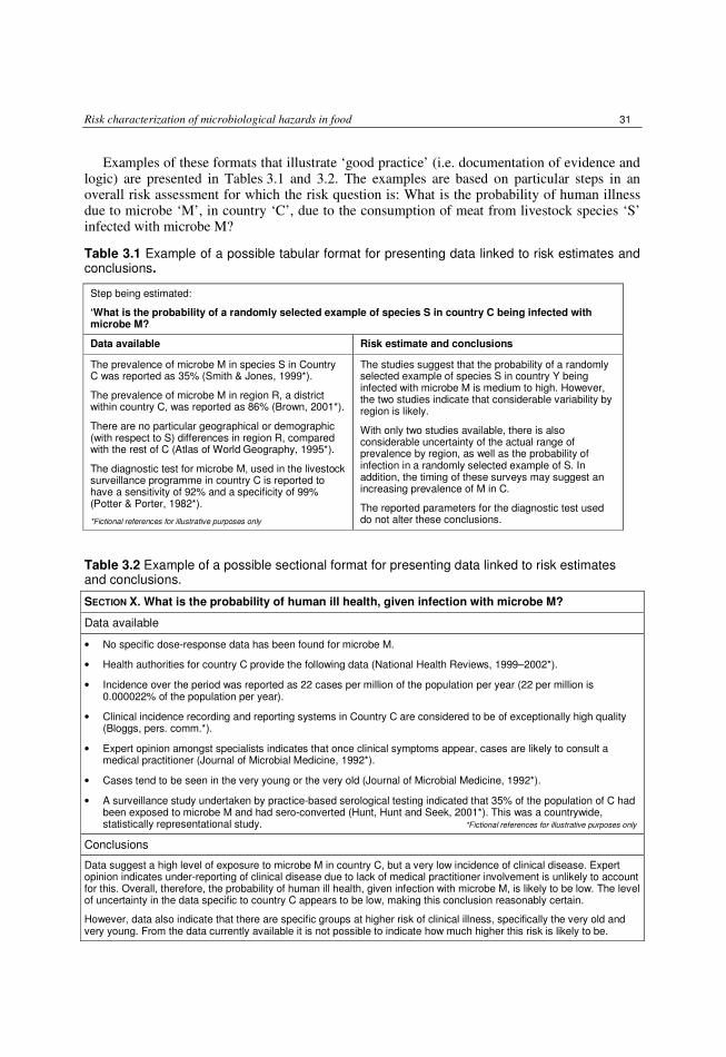
Risk characterization of microbiological hazards in food 31
Examples of these formats that illustrate ‘good practice’ (i.e. documentation of evidence and logic) are presented in Tables 3.1 and 3.2. The examples are based on particular steps in an overall risk assessment for which the risk question is: What is the probability of human illness due to microbe ‘M’, in country ‘C’, due to the consumption of meat from livestock species ‘S’ infected with microbe M?
Table 3.1 Example of a possible tabular format for presenting data linked to risk estimates and conclusions.
Step being estimated:
‘What is the probability of a randomly selected example of species S in country C being infected with microbe M?
Data available Risk estimate and conclusions
The prevalence of microbe M in species S in Country C was reported as 35% (Smith & Jones, 1999*).
The prevalence of microbe M in region R, a district within country C, was reported as 86% (Brown, 2001*).
There are no particular geographical or demographic (with respect to S) differences in region R, compared with the rest of C (Atlas of World Geography, 1995*).
The diagnostic test for microbe M, used in the livestock surveillance programme in country C is reported to have a sensitivity of 92% and a specificity of 99% (Potter & Porter, 1982*).
*Fictional references for illustrative purposes only
The studies suggest that the probability of a randomly selected example of species S in country Y being infected with microbe M is medium to high. However, the two studies indicate that considerable variability by region is likely.
With only two studies available, there is also considerable uncertainty of the actual range of prevalence by region, as well as the probability of infection in a randomly selected example of S. In addition, the timing of these surveys may suggest an increasing prevalence of M in C.
The reported parameters for the diagnostic test used do not alter these conclusions.
Table 3.2 Example of a possible sectional format for presenting data linked to risk estimates and conclusions.
SECTION X. What is the probability of human ill health, given infection with microbe M?
Data available
• No specific dose-response data has been found for microbe M.
• Health authorities for country C provide the following data (National Health Reviews, 1999–2002*).
• Incidence over the period was reported as 22 cases per million of the population per year (22 per million is 0.000022% of the population per year).
• Clinical incidence recording and reporting systems in Country C are considered to be of exceptionally high quality (Bloggs, pers. comm.*).
• Expert opinion amongst specialists indicates that once clinical symptoms appear, cases are likely to consult a medical practitioner (Journal of Microbial Medicine, 1992*).
• Cases tend to be seen in the very young or the very old (Journal of Microbial Medicine, 1992*).
• A surveillance study undertaken by practice-based serological testing indicated that 35% of the population of C had been exposed to microbe M and had sero-converted (Hunt, Hunt and Seek, 2001*). This was a countrywide, statistically representational study. *Fictional references for illustrative purposes only
Conclusions
Data suggest a high level of exposure to microbe M in country C, but a very low incidence of clinical disease. Expert opinion indicates under-reporting of clinical disease due to lack of medical practitioner involvement is unlikely to account for this. Overall, therefore, the probability of human ill health, given infection with microbe M, is likely to be low. The level of uncertainty in the data specific to country C appears to be low, making this conclusion reasonably certain.
However, data also indicate that there are specific groups at higher risk of clinical illness, specifically the very old and very young. From the data currently available it is not possible to indicate how much higher this risk is likely to be.

32 Qualitative risk characterization in risk assessment
3.4 Examples of qualitative risk assessment
A number of existing, published, qualitative risk characterizations are presented below.
3.4.1 WHO faecal pollution and water quality
The ‘Annapolis Protocol’ (WHO, 1999) was developed in response to concerns regarding the adequacy and effectiveness of approaches to monitoring and management of faecally-polluted recreational waters. One of the most important changes recommended in the Annapolis Protocol was a move away from sole reliance on ‘guideline’ values of faecal indicator bacteria to the use of a qualitative ranking of faecal loading in recreational-water environments. The protocol was tested in several countries, and an expert consultation was convened by WHO (WHO, 2001) to update the draft 1998 WHO Guidelines for Safe Recreational-water Environments. A revised Chapter 4 in Volume 1 of the guidelines was produced from the expert consultation, which described a suitable approach to risk assessment and risk management (WHO, 2003). Tables were produced for water bodies affected by three different sources of human faecal contamination: sewage outfalls, riverine discharges and bather shedding. The tables were based on qualitative assessment of risk of exposure under ‘normal’ conditions of sewage operation, water levels, etc, and classified the potential human risk. Table 3.3 reproduces the classification for sewage outfalls.
Table 3.3 Relative risk potential to human health through exposure to sewage through outfalls (reproduced from WHO, 2003).
Discharge type Treatment
Directly on beach Short outfalla Effective outfallb
Nonec Very High High NAd
Preliminary Very High High Low
Primary (including septic tank) Very High High Low
Secondary High High Low
Secondary plus disinfectione Moderate Moderate Very Low
Tertiary Moderate Moderate Very Low
Tertiary plus disinfection Very Low Very Low Very Low
Lagoons High High Low
Notes: (a) The relative risk is modified by population size. Relative risk is increased for discharges from large populations and decreased for discharges from small populations. (b) This assumes that the design capacity has not been exceeded and that climatic and oceanic extreme conditions are considered in the design objective (i.e. no sewage on the beach zone). (c) Includes combined sewer overflows. (d) NA = not applicable. (e) Additional investigations recommended to account for the likely lack of prediction with faecal index organisms
Risk characterization of microbiological hazards in food 33
3.4.2 Australian Drinking Water Guidelines
As part of Australia’s National Water Quality Management Strategy the Australian National Health and Medical Research Council produced the Australia Drinking Water Guidelines (NHMRC, 2004) as a framework for good management of drinking water supplies. The guidelines are not mandatory standards, but are designed to provide an authoritative reference document and framework for good management of drinking water supplies to assure safety at point of use by consumers in all parts of Australia. The guidelines consider that the greatest risks to consumers of drinking water are pathogenic microorganisms, and as such covers similar issues for water that microbiological food safety risk assessment covers for food, although it should be noted that the issue of microbiological growth and inactivation (through food processing) are likely to play a much larger role in microbiological food safety risk assessment. The extensive guidelines document includes a qualitative method for assessing human health risks and recommends that risks should be assessed at two levels:
• Maximum risk in the absence of preventive measures (equivalent to ‘unrestricted risk’ as described in Section 2.3.1); and
• Residual risk after consideration of existing preventive measures.
The level of risk of each hazard (pathogen, or hazardous event) is qualitatively assessed by combining a qualitative assessment of the likelihood of the hazard occurring, and the severity of the consequences if it were to occur, according to Tables 3.4a–c (Tables 3.1, 3.2 and 3.3 in the original document), which were developed from the Australian/New Zealand risk analysis standard ‘AS/NZS 4360:1999: Risk management’, which has since been superseded (AS/NZS 4360:2004). The guidelines document also includes what are essentially qualitative hazard identification and hazard characterizations for a wide range of water-borne hazards that can be used to assist in the application of the risk matrices. The stated aim of the methodology is “to distinguish between very high and low risks” (NHMRC, 2004).
3.4.3 EFSA BSE/TSE risk assessment of goat milk and milk-derived products
A research group in France found a suspected case of Bovine Spongiform Encephalopathy (BSE) infection in a slaughtered goat in 2002. As a result, the European Commission (EC) requested advice from the European Food Safety Authority (EFSA) on the safety of milk and meat in relation to Transmissible Spongiform Encephalopathy (TSE) in goats and sheep. EFSA (2004a) published the following preliminary statement:
“From the limited data available today it is concluded that in the light of current scientific knowledge and irrespective of their geographical origin, milk and milk derivatives (e.g. lactoferrin, lactose) from small ruminants are unlikely to present any risk of TSE contamination provided that milk is sourced from clinically healthy animals. Exclusion of animals with mastitis is considered to reduce the potential risk. Further assurance of healthy milk could include milk tests for total somatic cell counts indicative of inflammation.” [Emphasis added].
EFSA also commented (EFSA Press release 713):
“A comprehensive and quantitative assessment of the risks involved in the consumption of goat meat, milk and dairy products will only be possible if more scientific research data on the occurrence of TSE in small ruminants can be obtained. Such a quantitative risk assessment, if feasible, will take considerably more time.”

34 Qualitative risk characterization in risk assessment
Table 3.4a Qualitative measures of likelihood.
Level Descriptor Example description
A Almost certain Is expected to occur in most circumstances
B Likely Will probably occur in most circumstances
C Possible Might occur or should occur at some time
D Unlikely Could occur at some time
E Rare May occur only in exceptional circumstances
Table 3.4b Qualitative measures of consequence or impact.
Level Descriptor Example description
1 Insignificant Insignificant impact; little disruption to normal operation; low increase in normal operation costs
2 Minor Minor impact for small population; some manageable operation disruption; some increase in operating costs
3 Moderate Minor impact for large population; significant modification to normal operation but manageable; operation costs increased; increased monitoring
4 Major Major impact for small population; systems significantly compromised and abnormal operation, if at all; high level of monitoring required
5 Catastrophic Major impact for large population; complete failure of systems
Table 3.4c Qualitative risk analysis matrix: level of risk.
Consequences Likelihood
1 Insignificant 2 Minor 3 Moderate 4 Major 5 Catastrophic
A (almost certain) Moderate High Very high Very high Very high
B (likely) Moderate High High Very high Very high
C (possible) Low Moderate High Very high Very high
D (unlikely) Low Low Moderate High Very high
E (rare) Low Low Moderate High High
It is extremely difficult to assess the risk of BSE-contaminated product because there is no means to measure the number of prions present in a food product, and no human-dose-response relationship for prion levels. EFSA nonetheless needed to provide comment on the level of the above risk, and relied on an expert panel to review the available data.
3.4.4 Geographical BSE cattle risk assessment
In 2003, EFSA was requested by the EC to re-assess geographical BSE risk (GBR) and concluded the following (EFSA 2004b):
“1. The Geographical BSE-Risk (GBR) is a qualitative indicator of the likelihood of the presence of one or more cattle being infected with BSE, pre-clinically as well as clinically, at a given point in time, in a country. Where its presence is confirmed, the GBR gives an indication of the level of infection.

Risk characterization of microbiological hazards in food 35
2. The GBR assessments are based on information submitted by countries concerned in response to a European Commission recommendation in 1998 setting out the information requirements for such an assessment. The information concerns in particular imports of bovines and meat and bone meal (MBM) from the United Kingdom and other BSE-risk countries, rendering standards for animal by-products, use of so called Specified Risk Materials (SRMs), feeding of MBM to ruminants, etcetera.
3. Table 3.5 shows the current GBR levels of the seven countries assessed by EFSA so far, as well as their former classification where available. "
Table 3.5 Geographical BSE Risk (GBR) in 2003 in seven countries as assessed by EFSA (2004b). Earlier assessed levels are also shown.
GBR level
Presence of one or more cattle clinically or pre-clinically infected with the BSE agent in a geographical region or country
GBR of the country or region Current status (status before)
I Highly unlikely Australia (I)
II Unlikely but not excluded Norway (I), Sweden (II)
III Likely but not confirmed or confirmed at a lower level Canada (II), Mexico (N/A), South Africa (N/A), USA (II)
IV Confirmed at a higher level none
NOTES: N/A = not applicable, i.e. not assessed before”

4. Semi-quantitative risk characterization
4.1 Introduction
Semi-quantitative risk assessment provides an intermediary level between the textual evaluation of qualitative risk assessment and the numerical evaluation of quantitative risk assessment, by evaluating risks with a score. It offers a more consistent and rigorous approach to assessing and comparing risks and risk management strategies than does qualitative risk assessment, and avoids some of the greater ambiguities that a qualitative risk assessment may produce. It does not require the same mathematical skills as quantitative risk assessment, nor does it require the same amount of data, which means it can be applied to risks and strategies where precise data are missing. Nonetheless, all forms of risk assessment require the greatest possible collection and evaluation of data available on the risk issue, and food safety risk assessments require in-depth knowledge in a variety of scientific disciplines. Semi-quantitative risk assessment requires all of the data collection and analysis activities for qualitative risk assessment as described in the previous chapter.
Semi-quantitative risk assessment is a relatively new idea in food safety. Codex Alimentarius Commission (CAC) and others generally consider just two categories of risk assessment: qualitative and quantitative. Semi-quantitative risk assessment, as described here, has often been grouped together with qualitative risk assessment, but this understates the important differences between them in their structure and their relative levels of objectivity, transparency and repeatability.
4.1.1 Uses of semi-quantitative risk assessment
Semi-quantitative risk assessment is most useful in providing a structured way to rank risks according to their probability, impact or both (severity), and for ranking risk reduction actions for their effectiveness. This is achieved through a predefined scoring system that allows one to map a perceived risk into a category, where there is a logical and explicit hierarchy between categories.
Semi-quantitative risk assessment is generally used where one is attempting to optimize the allocation of available resources to minimize the impact of a group of risks under the control of one organization. It helps achieve this in two ways: first the risks can be placed onto a sort of map so that the most important risks can be separated from the less important; second, by comparing the total score for all risks before and after any proposed risk reduction strategy (or combination of strategies) one can get a feel for how relatively effective the strategies are and whether they merit their costs. Semi-quantitative risk assessment has been used with great success in various arenas of project and military risk for over a decade, and is beginning to find favour in foodborne pathogen-related areas.
Semi-quantitative risk assessment offers the advantage of being able to evaluate a larger number of risk issues than quantitative risk assessment because a full mathematical model is not necessary. The results of fully quantitative risk assessments, where they have been possible, can be included in a semi-quantitative rationale, although usually at the loss of some quantitative precision, as the more precise enumeration of probability and impact from the quantitative risk assessment has to be placed into categories that cover broad ranges of probability and impact.
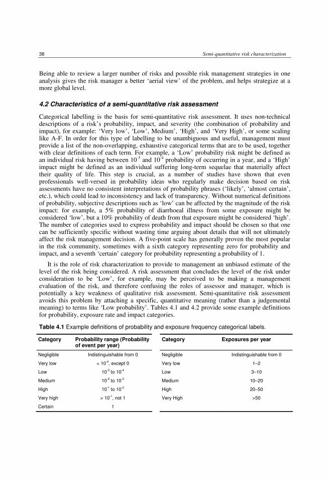
38 Semi-quantitative risk characterization
Being able to review a larger number of risks and possible risk management strategies in one analysis gives the risk manager a better ‘aerial view’ of the problem, and helps strategize at a more global level.
4.2 Characteristics of a semi-quantitative risk assessment
Categorical labelling is the basis for semi-quantitative risk assessment. It uses non-technical descriptions of a risk’s probability, impact, and severity (the combination of probability and impact), for example: ‘Very low’, ‘Low’, Medium’, ‘High’, and ‘Very High’, or some scaling like A-F. In order for this type of labelling to be unambiguous and useful, management must provide a list of the non-overlapping, exhaustive categorical terms that are to be used, together with clear definitions of each term. For example, a ‘Low’ probability risk might be defined as an individual risk having between 10-3 and 10-4 probability of occurring in a year, and a ‘High’ impact might be defined as an individual suffering long-term sequelae that materially affect their quality of life. This step is crucial, as a number of studies have shown that even professionals well-versed in probability ideas who regularly make decision based on risk assessments have no consistent interpretations of probability phrases (‘likely’, ‘almost certain’, etc.), which could lead to inconsistency and lack of transparency. Without numerical definitions of probability, subjective descriptions such as ‘low’ can be affected by the magnitude of the risk impact: for example, a 5% probability of diarrhoeal illness from some exposure might be considered ‘low’, but a 10% probability of death from that exposure might be considered ‘high’. The number of categories used to express probability and impact should be chosen so that one can be sufficiently specific without wasting time arguing about details that will not ultimately affect the risk management decision. A five-point scale has generally proven the most popular in the risk community, sometimes with a sixth category representing zero for probability and impact, and a seventh ‘certain’ category for probability representing a probability of 1.
It is the role of risk characterization to provide to management an unbiased estimate of the level of the risk being considered. A risk assessment that concludes the level of the risk under consideration to be ‘Low’, for example, may be perceived to be making a management evaluation of the risk, and therefore confusing the roles of assessor and manager, which is potentially a key weakness of qualitative risk assessment. Semi-quantitative risk assessment avoids this problem by attaching a specific, quantitative meaning (rather than a judgemental meaning) to terms like ‘Low probability’. Tables 4.1 and 4.2 provide some example definitions for probability, exposure rate and impact categories.
Table 4.1 Example definitions of probability and exposure frequency categorical labels.
Category Probability range (Probability of event per year)
Category Exposures per year
Negligible Indistinguishable from 0 Negligible Indistinguishable from 0
Very low < 10-4, except 0 Very low 1–2
Low 10-3 to 10-4 Low 3–10
Medium 10-2 to 10-3 Medium 10–20
High 10-1 to 10-2 High 20–50
Very high > 10-1, not 1 Very High >50
Certain 1
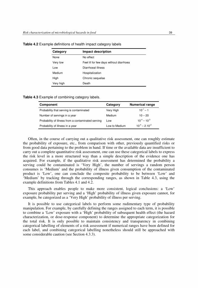
Risk characterization of microbiological hazards in food 39
Table 4.2 Example definitions of health impact category labels
Category Impact description
None No effect
Very low Feel ill for few days without diarrhoea
Low Diarrhoeal illness
Medium Hospitalization
High Chronic sequelae
Very high Death
Table 4.3 Example of combining category labels.
Component Category Numerical range
Probability that serving is contaminated Very High 10-1 – 1
Number of servings in a year Medium 10 – 20
Probability of illness from a contaminated serving Low 10-4 – 10-3
Probability of illness in a year Low to Medium 10-4 – 2.10-2
Often, in the course of carrying out a qualitative risk assessment, one can roughly estimate the probability of exposure, etc., from comparison with other, previously quantified risks or from good data pertaining to the problem in hand. If time or the available data are insufficient to carry out a complete quantitative risk assessment, one can use these categorical labels to express the risk level in a more structured way than a simple description of the evidence one has acquired. For example, if the qualitative risk assessment has determined the probability a serving could be contaminated is ‘Very High’, the number of servings a random person consumes is ‘Medium’ and the probability of illness given consumption of the contaminated product is ‘Low’, one can conclude the composite probability to be between ‘Low’ and ‘Medium’ by tracking through the corresponding ranges, as shown in Table 4.3, using the example definitions from Tables 4.1 and 4.2.
This approach enables people to make more consistent, logical conclusions: a ‘Low’ exposure probability per serving and a ‘High’ probability of illness given exposure cannot, for example, be categorized as a ‘Very High’ probability of illness per serving.
It is possible to use categorical labels to perform some rudimentary type of probability manipulation. For example, by carefully defining the ranges assigned to each term, it is possible to combine a ‘Low’ exposure with a ‘High’ probability of subsequent health effect (the hazard characterization, or dose-response component) to determine the appropriate categorization for the total risk. It is only possible to maintain consistency and transparency in combining categorical labelling of elements of a risk assessment if numerical ranges have been defined for each label, and combining categorical labelling nonetheless should still be approached with some considerable caution (see Section 4.3.3).

40 Semi-quantitative risk characterization
4.3 Performing a semi-quantitative risk assessment
A P-I (probability-impact) table offers a quick way to visualize the relative riskiness or severity (a common term in risk analysis for the combination of probability and impact) of all identified risks within the domain of analysis. Table 4.4 illustrates an example. All risks (e.g. the list of pathogens that might appear in a particular food type) are plotted in the one table, allowing for the easy identification of the most threatening risks as well as providing a general picture of the overall risk associated with the food type. The numbers in the table are indices for identified risks. Risks 2 and 13, for example, have high severity; risks 3, 5 and 7 have very low severity. Risks with zero events per year (i.e. zero probability, e.g. risks 11 and 14) or zero impact (e.g. risks 8, 9 and 10) are not strictly risks, but may be useful to document in a P-I table as having been identified and subsequently determined to be negligible.
Table 4.4 Example of a P-I table for individual risk per year.
I VHI 6 13,2
M HI 14 15 12
P MED 5 4 1
A LO
C VLO 11 7 3
T NIL 8,9 10
NIL VLO LO MED HI VHI EVENTS PER YEAR
Severity scores (sometimes called P-I scores) can be used to rank the identified risks. A scaling factor, or score, is assigned to each label used to describe each type of impact. If a log scale is used to define each categorical scale, as in the examples provided in Table 4.1 for probability and Table 4.2 for impact (one could debate whether there was a log of difference between each impact category and adjust if necessary), the probability and impact scores can be designed such that the severity score of a risk is then the sum of the probability and impact scores, or some other simple mathematical equation. Table 4.5 provides an example of the type of scaling factors that could be associated with each term and impact type combination.
In this example (Table 4.5), an impact of 6 has been given for ‘Very High’ as this refers to death, which is a much greater leap from chronic sequelae than chronic sequelae is from hospitalization, or any of the other impact increments. The risks of Table 4.4 can now be assigned a severity score, such as that shown in Table 4.6 (where probability and rate as considered equivalent).
Severity scores enable the risks to be categorized and ranked according to severity. In the scoring regime of Table 4.5, for example, a ‘High’ severity risk could be defined as having a score greater than 7, a ‘Medium’ severity risk as having a score between 4 and 6 and a ‘Low’ severity risk as having a score less than 4. A key drawback to this approach of ranking risks is that the process is very sensitive to the scaling factors that are assigned to each term describing the risk impacts.

Risk characterization of microbiological hazards in food 41
Table 4.5 Example of the type of scaling factors that can be applied to determine a severity score.
Rating Probability score Impact scoreNone NA NAVLO 1 1LO 2 2
MED 3 3HI 4 4
VHI 5 6
Table 4.6 Example severity score calculations for risks from Table 4.4.
Risk index Probability Probability score Impact Impact score Severity score
13 VHI 5 VHI 6 5+6 = 11
1 HI 4 MED 3 4+3 = 7
5 VLO 1 MED 3 1+3 = 4
4.3.1 Risks with several impact dimensions
The usual endpoint of a microbiological food safety risk assessment is some measure of human health risk. However, an analysis may consider other types of impact, like economic loss or erosion of quality of life (e.g. reduction in choice of ‘safe’ food products), some of which have less numerically definable impacts.
P-I tables can be constructed in a number of ways: for example, displaying the various types of impact of each individual risk (such as for a particular bacterium, or a particular food product). Table 4.7 is an example where the human health impact (H), cost (£) and social (S) impact are shown for a specific risk. The probability of each impact may not be the same. In this example, the probability of the risk event occurring is ‘high’ and if it occurs is certain to result in a cost impact. There is a smaller probability of a health impact, and it is considered that there is a ‘low’ probability of the event occurring and producing a social impact. Implicit in assigning categories for more than one type of impact is that one has assigned broad correspondence in value between, for example, human health impact and economic loss.
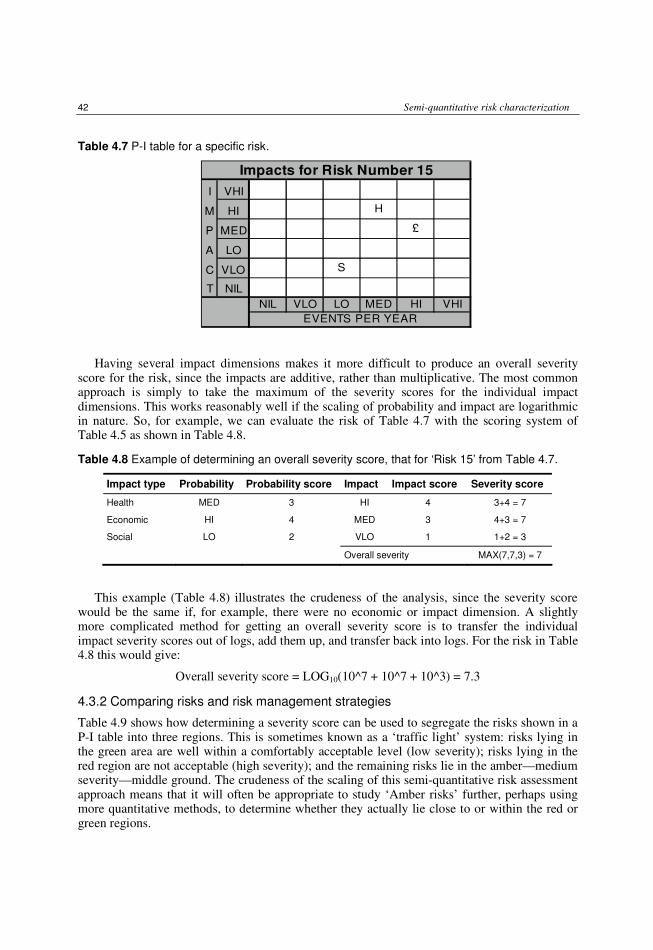
42 Semi-quantitative risk characterization
Table 4.7 P-I table for a specific risk.
Impacts for Risk Number 15
I VHI
M HI H
P MED £
A LO
C VLO S
T NIL NIL VLO LO MED HI VHI EVENTS PER YEAR
Having several impact dimensions makes it more difficult to produce an overall severity score for the risk, since the impacts are additive, rather than multiplicative. The most common approach is simply to take the maximum of the severity scores for the individual impact dimensions. This works reasonably well if the scaling of probability and impact are logarithmic in nature. So, for example, we can evaluate the risk of Table 4.7 with the scoring system of Table 4.5 as shown in Table 4.8.
Table 4.8 Example of determining an overall severity score, that for ‘Risk 15’ from Table 4.7.
Impact type Probability Probability score Impact Impact score Severity score
Health MED 3 HI 4 3+4 = 7
Economic HI 4 MED 3 4+3 = 7
Social LO 2 VLO 1 1+2 = 3
Overall severity MAX(7,7,3) = 7
This example (Table 4.8) illustrates the crudeness of the analysis, since the severity score would be the same if, for example, there were no economic or impact dimension. A slightly more complicated method for getting an overall severity score is to transfer the individual impact severity scores out of logs, add them up, and transfer back into logs. For the risk in Table 4.8 this would give:
Overall severity score = LOG10(10^7 + 10^7 + 10^3) = 7.3
4.3.2 Comparing risks and risk management strategies
Table 4.9 shows how determining a severity score can be used to segregate the risks shown in a P-I table into three regions. This is sometimes known as a ‘traffic light’ system: risks lying in the green area are well within a comfortably acceptable level (low severity); risks lying in the red region are not acceptable (high severity); and the remaining risks lie in the amber—medium severity—middle ground. The crudeness of the scaling of this semi-quantitative risk assessment approach means that it will often be appropriate to study ‘Amber risks’ further, perhaps using more quantitative methods, to determine whether they actually lie close to or within the red or green regions.
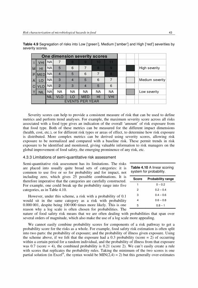
Risk characterization of microbiological hazards in food 43
Table 4.9 Segregation of risks into Low [‘green’], Medium [‘amber’] and High [‘red’] severities by severity scores.
One dimension severity scores
I VHI NA 7 8 9 10 11
M HI NA 5 6 7 8 9 High severity
P MED NA 4 5 6 7 8
A LO NA 3 4 5 6 7 Medium severity
C VLO NA 2 3 4 5 6
T NIL NA NA NA NA NA NA Low severity
NIL VLO LO MED HI VHI EVENTS PER YEAR
Severity scores can help to provide a consistent measure of risk that can be used to define metrics and perform trend analyses. For example, the maximum severity score across all risks associated with a food type gives an indication of the overall ‘amount’ of risk exposure from that food type. Both of these metrics can be measured for the different impact dimensions (health, cost, etc.), or for different risk types or areas of effect, to determine how risk exposure is distributed. More complex metrics can be derived using severity scores, allowing risk exposure to be normalized and compared with a baseline risk. These permit trends in risk exposure to be identified and monitored, giving valuable information to risk managers on the global improvement of food safety, the emerging prominence of any risk, etc.
4.3.3 Limitations of semi-quantitative risk assessment
Semi-quantitative risk assessment has its limitations. The risks are placed into usually quite broad sets of categories: it is common to use five or so for probability and for impact, not including zero, which gives 25 possible combinations. It is therefore imperative that the categories are carefully constructed. For example, one could break up the probability range into five categories, as in Table 4.10.
However, under this scheme, a risk with a probability of 0.1 would sit in the same category as a risk with probability 0.000 001, despite being 100 000 times more likely. This is one reason why a log scale is often chosen for probabilities. The nature of food safety risk means that we are often dealing with probabilities that span over several orders of magnitude, which also make the use of a log scale more appealing.
We cannot easily combine probability scores for components of a risk pathway to get a probability score for the risks as a whole. For example, food safety risk estimation is often split into two parts: the probability of exposure; and the probability of illness given exposure. Using the scheme above, if we felt that the exposure had a 0.3 probability (score = 2) of occurring within a certain period for a random individual, and the probability of illness from that exposure was 0.7 (score = 4), the combined probability is 0.21 (score 2). We can’t easily create a rule with scores that replicates the probability rules. Taking the minimum of the two scores is one partial solution (in Excel®, the syntax would be MIN(2,4) = 2) but this generally over-estimates
Table 4.10 A linear scoring system for probability.
Score Probability range
1 0 – 0.2
2 0.2 – 0.4
3 0.4 – 0.6
4 0.6 – 0.8
5 0.8 – 1
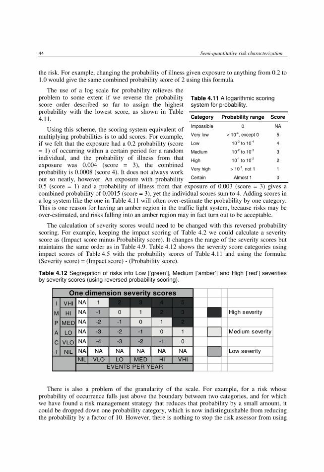
44 Semi-quantitative risk characterization
the risk. For example, changing the probability of illness given exposure to anything from 0.2 to 1.0 would give the same combined probability score of 2 using this formula.
The use of a log scale for probability relieves the problem to some extent if we reverse the probability score order described so far to assign the highest probability with the lowest score, as shown in Table 4.11.
Using this scheme, the scoring system equivalent of multiplying probabilities is to add scores. For example, if we felt that the exposure had a 0.2 probability (score = 1) of occurring within a certain period for a random individual, and the probability of illness from that exposure was 0.004 (score = 3), the combined probability is 0.0008 (score 4). It does not always work out so neatly, however. An exposure with probability 0.5 (score = 1) and a probability of illness from that exposure of 0.003 (score = 3) gives a combined probability of 0.0015 (score = 3), yet the individual scores sum to 4. Adding scores in a log system like the one in Table 4.11 will often over-estimate the probability by one category. This is one reason for having an amber region in the traffic light system, because risks may be over-estimated, and risks falling into an amber region may in fact turn out to be acceptable.
The calculation of severity scores would need to be changed with this reversed probability scoring. For example, keeping the impact scoring of Table 4.2 we could calculate a severity score as (Impact score minus Probability score). It changes the range of the severity scores but maintains the same order as in Table 4.9. Table 4.12 shows the severity score categories using impact scores of Table 4.5 with the probability scores of Table 4.11 and using the formula: (Severity score) = (Impact score) - (Probability score).
Table 4.12 Segregation of risks into Low [‘green’], Medium [‘amber’] and High [‘red’] severities by severity scores (using reversed probability scoring).
One dimension severity scores
I VHI NA 1 2 3 4 5
M HI NA -1 0 1 2 3 High severity
P MED NA -2 -1 0 1 2
A LO NA -3 -2 -1 0 1 Medium severity
C VLO NA -4 -3 -2 -1 0
T NIL NA NA NA NA NA NA Low severity
NIL VLO LO MED HI VHI EVENTS PER YEAR
There is also a problem of the granularity of the scale. For example, for a risk whose probability of occurrence falls just above the boundary between two categories, and for which we have found a risk management strategy that reduces that probability by a small amount, it could be dropped down one probability category, which is now indistinguishable from reducing the probability by a factor of 10. However, there is nothing to stop the risk assessor from using
Table 4.11 A logarithmic scoring system for probability.
Category Probability range Score
Impossible 0 NA
Very low < 10-4, except 0 5
Low 10-3 to 10-4 4
Medium 10-2 to 10-3 3
High 10-1 to 10-2 2
Very high > 10-1, not 1 1
Certain Almost 1 0

Risk characterization of microbiological hazards in food 45
score fractions if it seems appropriate. The integer system is designed for convenience and simplicity, and should be changed to include fractions if this better represents the available knowledge.
Using the semi-quantitative risk assessment scoring system as a surrogate for probability calculations is also likely to cause more severe inaccuracies when one assesses a longer sequence of events.
4.3.4 Dealing with uncertainty and variability
In one sense the broad category ranges assigned to probability and impact scales make it less essential to consider anything but large-scale uncertainty. The overview nature of semi-quantitative risk assessment also helps one think about more global issues of model uncertainty. That said, quantitative food safety risk assessment results that are not anchored to correspond to observed illness rates frequently span several orders of magnitude of uncertainty. The level of available information may also make it difficult to assign probability and impact categories to a particular risk. It would be useful and more objective to be able to express this uncertainty. One method is to describe the uncertainty by showing a risk as lying within an area of the P-I table, as in Table 4.13.
Table 4.13 Graphically expressing uncertainty about a risk category.
I VHI
M HI
P MED 4
A LO
C VLO
T NIL NIL VLO LO MED HI VHI EVENTS PER YEAR
Here, the (optional) darker shading represents where the risk assessment team feel the risk most likely lies, and the lighter shading represents the range of uncertainty about that evaluation. Graphical shapes, like circles, drawn on the table to represent uncertainty make it easier to plot several risks together.
One can also employ standard Monte Carlo simulation to express uncertainty in scores where they are being manipulated in more mathematical analyses discussed above.
Variability, such as variability in susceptibility between subpopulations, can easily be incorporated in semi-quantitative risk assessment (where the necessary data are available) by estimating the risk for subpopulations and plotting them separately on the same chart. This provides an excellent overview of how different subpopulations share the food safety risk.
4.3.5 Data requirements
The basic principle of risk assessment is to collect as much data as you can, providing that the inclusion of more data may affect the decision being made. The data collected for a qualitative risk assessment are often sufficient for semi-quantitative risk assessment needs. The difference
46 Semi-quantitative risk characterization
between the two is that semi-quantitative risk assessment has a greater focus on attempting to evaluate the components of the risk to within defined quantitative bounds. Thus, at times, one may do a statistical analysis on a data set to attempt to more precisely estimate a probability, or the expected impact, providing it will give the assessor more confidence about how to categorize the risk.
Semi-quantitative risk assessment is usually used as a means to compare several risks or risk management strategies. At times we may have sufficient data to be able to perform a full quantitative risk assessment for a select number of risks (e.g. food–pathogen combinations). A quantitative model can give us more information about specific strategies to apply to that particular risk issue, but we can also use the quantitative results to place these more precisely evaluated risks into context with others of concern in a semi-quantitative environment.
4.3.6 Transparency in reaching conclusions
Semi-quantitative risk assessment offers a lot of advantages in achieving transparency. No sophisticated mathematical model is necessary, for example, which is appealing to the lay person. However, the use of mathematical models as an obstacle to transparency may be over-emphasized. Most food safety risk assessments require understanding of complex microbiological information and usually a reasonable level of human medicine, and of epidemiological principles which tend to be postgraduate topics, whereas quantitative risk assessment uses mathematics generally covered at undergraduate level. The main obstacle to transparency of quantitative models is that there are only a few people who have specialized in the field.
Semi-quantitative risk assessment encourages the development of decision rules (e.g. the traffic-light system) that can be easily followed and checked. The framework for placing risks within a P-I table makes it much easier to demonstrate a consistency in handling risks because they are all analysed together.
The key transparency issue with semi-quantitative risk assessment arises from the granularity of the scales used in scoring. The usually rather broad categories means that we lose any distinction between risks that can be considerably different in probability and/or impact magnitude. This means, for example, that one food industry could be unfairly penalized because its product lies just above a category, or that industries or regulator only have the incentive to push a risk just over the category boundary.
Semi-quantitative risk assessment is a system for sorting out risks, focusing on the big issues, and managing the entire risk portfolio better. The scoring system is inherently imperfect, but so is any other risk evaluation system. If the scoring system being used can be shown to produce important errors in decision logic, then one can use potentially more precise quantitative risk assessment arguments, or change the scoring system to something more precise.
4.4 Examples of semi-quantitative risk assessment
4.4.1 New Zealand risk profile of Mycobacterium bovis in milk
The New Zealand Food Safety Authority commissioned the New Zealand Institute of Environmental Science & Research Ltd (ESR) to provide a ‘Risk profile’ of Mycobacterium bovis in milk (Lake, Hudson and Cressey, 2002b).
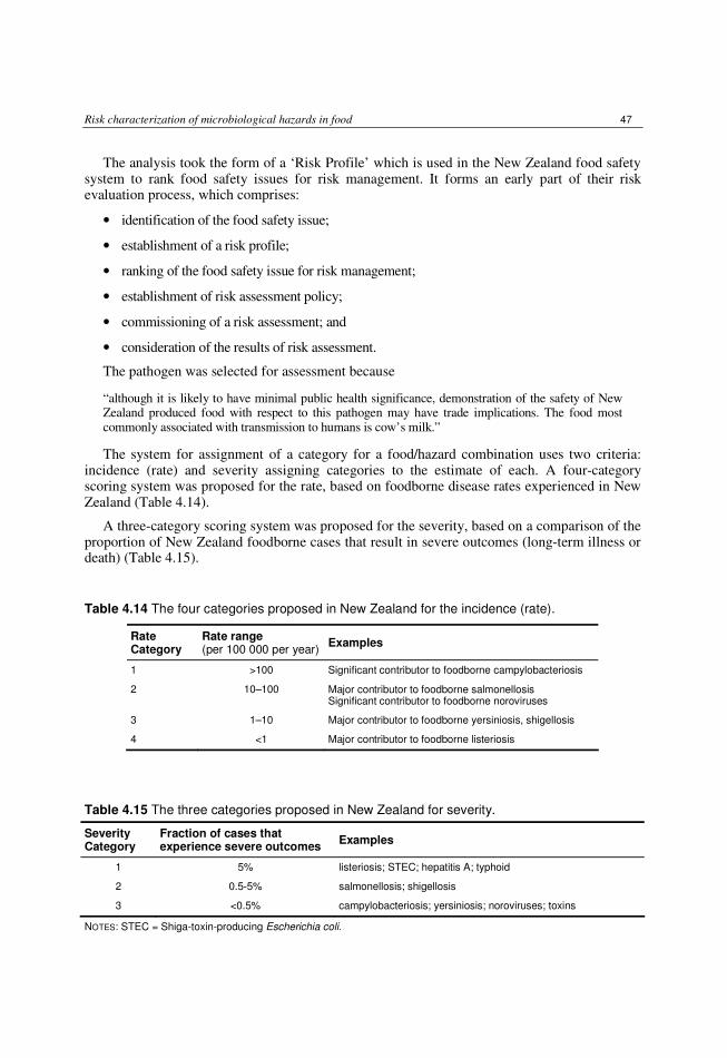
Risk characterization of microbiological hazards in food 47
The analysis took the form of a ‘Risk Profile’ which is used in the New Zealand food safety system to rank food safety issues for risk management. It forms an early part of their risk evaluation process, which comprises:
• identification of the food safety issue;
• establishment of a risk profile;
• ranking of the food safety issue for risk management;
• establishment of risk assessment policy;
• commissioning of a risk assessment; and
• consideration of the results of risk assessment.
The pathogen was selected for assessment because
“although it is likely to have minimal public health significance, demonstration of the safety of New Zealand produced food with respect to this pathogen may have trade implications. The food most commonly associated with transmission to humans is cow’s milk.”
The system for assignment of a category for a food/hazard combination uses two criteria: incidence (rate) and severity assigning categories to the estimate of each. A four-category scoring system was proposed for the rate, based on foodborne disease rates experienced in New Zealand (Table 4.14).
A three-category scoring system was proposed for the severity, based on a comparison of the proportion of New Zealand foodborne cases that result in severe outcomes (long-term illness or death) (Table 4.15).
Table 4.14 The four categories proposed in New Zealand for the incidence (rate).
Rate Category
Rate range (per 100 000 per year) Examples
1 >100 Significant contributor to foodborne campylobacteriosis
2 10–100 Major contributor to foodborne salmonellosis Significant contributor to foodborne noroviruses
3 1–10 Major contributor to foodborne yersiniosis, shigellosis
4 <1 Major contributor to foodborne listeriosis
Table 4.15 The three categories proposed in New Zealand for severity.
Severity Category
Fraction of cases that experience severe outcomes Examples
1 5% listeriosis; STEC; hepatitis A; typhoid
2 0.5-5% salmonellosis; shigellosis
3 <0.5% campylobacteriosis; yersiniosis; noroviruses; toxins
NOTES: STEC = Shiga-toxin-producing Escherichia coli.
48 Semi-quantitative risk characterization
Analysis for Mycobacterium bovis in milk was hampered by a complete lack of prevalence information, so it was considered impossible to make even qualitative statements of exposure. The only available dose-response data were from animal experiments from 1934 and earlier, making it meaningless to consider a usual food safety risk assessment of exposure and hazard characterization. The risk profile method is based solely on epidemiological data in an attempt to inform decision-makers of how important the issue is among other food safety issues that need to be managed. The analysis discussed the available evidence and gave the following scores:
• Severity: 1 (>5% serious outcomes)
• Incidence: 4 (<1 per 100 000 people per year)
• Trade importance: high
ESR produces a risk profile for Salmonella in poultry (whole and pieces) using the same methods, but with considerably more data available (Lake, Hudson and Cressey, 2002a). Note that the risk assessment titles described these as ‘qualitative’ risk assessments. However, the numerical definitions of the broad category bands would place these risk assessments within the range of semi-quantitative risk assessments as discussed in this document.
4.4.2 Seafood safety using RiskRanger
FAO (2004) discusses the continuum between qualitative and quantitative risk assessment for seafood, and introduces a semi-quantitative risk assessment method that has been coded into a freely-available prototype decision support software tool called RiskRanger (Ross and Sumner, 2002). The tool requires answers to 11 questions, which describe the factors from harvest to consumption that affect the food safety risk of seafood. The questions can be answered in either qualitative (with predetermined categories) or quantitative terms. Qualitative answers are converted to quantitative values according to sets of tables.
The model is intended to be population specific, so key inputs like total and/or region population size are required to be predefined, although user-defined values can also be input. A score is then calculated from the inputs, allowing the ranking of various food–pathogen combinations. The scoring system is designed to have a scale of 0 to 100, where 100 represents the worst imaginable scenario, i.e. that every member of the population consumes a lethal dose every day. A 0 score was arbitrarily set to equate to one mild diarrhoeal case per 100 billion people per hundred years, the logic being that the Earth’s population is significantly less than 100 billion, so one would not expect to see an occurrence of the risk anywhere within a person’s lifetime. The chosen range extends over 17.6 orders of magnitude, which equates to 100/17.6 ≈ 6 ‘risk ranking’ units for each factor of 10 between risks.
The method has been designed to screen risks and to screen major categories of risk management options. The spreadsheet interface allows a risk manager to instantaneously consider what-if scenarios that can stimulate discussion of possible risk management strategies. The simplicity and generic nature of the model means that its results remain fairly crude. It also means that the questions that are posed are of a very general nature. The authors go into considerable detail to warn the reader of these limitations. There is, for example, no incorporation of uncertainty and variability in the model, though this could be readily added into the spreadsheet model using Monte Carlo simulation.
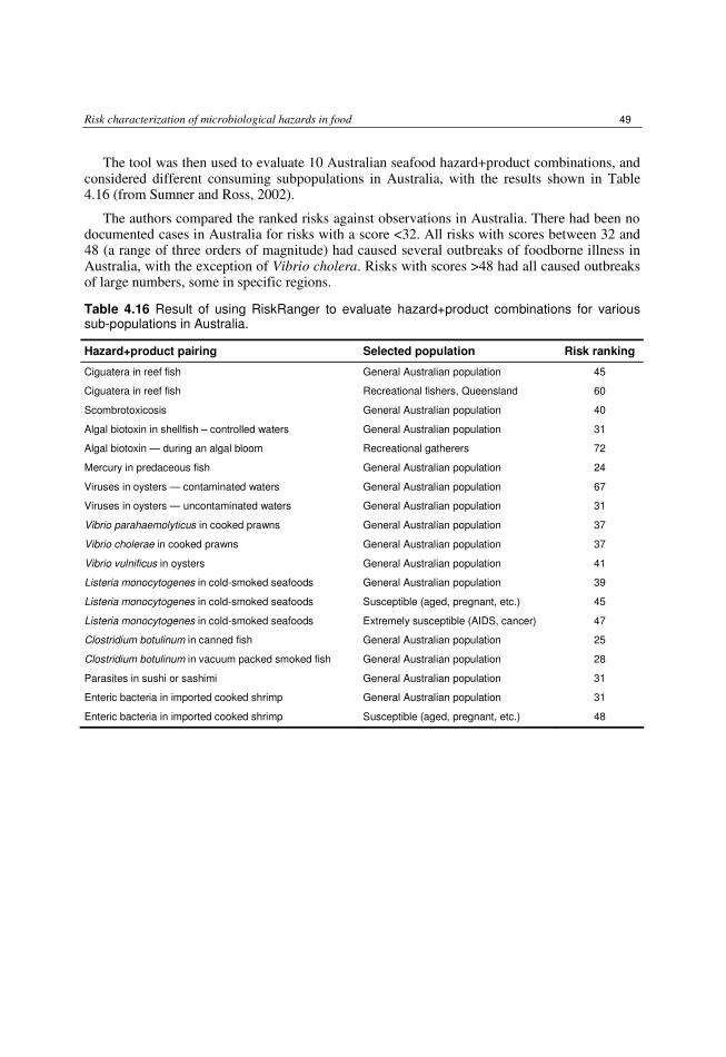
Risk characterization of microbiological hazards in food 49
The tool was then used to evaluate 10 Australian seafood hazard+product combinations, and considered different consuming subpopulations in Australia, with the results shown in Table 4.16 (from Sumner and Ross, 2002).
The authors compared the ranked risks against observations in Australia. There had been no documented cases in Australia for risks with a score <32. All risks with scores between 32 and 48 (a range of three orders of magnitude) had caused several outbreaks of foodborne illness in Australia, with the exception of Vibrio cholera. Risks with scores >48 had all caused outbreaks of large numbers, some in specific regions.
Table 4.16 Result of using RiskRanger to evaluate hazard+product combinations for various sub-populations in Australia.
Hazard+product pairing Selected population Risk ranking
Ciguatera in reef fish General Australian population 45
Ciguatera in reef fish Recreational fishers, Queensland 60
Scombrotoxicosis General Australian population 40
Algal biotoxin in shellfish – controlled waters General Australian population 31
Algal biotoxin — during an algal bloom Recreational gatherers 72
Mercury in predaceous fish General Australian population 24
Viruses in oysters — contaminated waters General Australian population 67
Viruses in oysters — uncontaminated waters General Australian population 31
Vibrio parahaemolyticus in cooked prawns General Australian population 37
Vibrio cholerae in cooked prawns General Australian population 37
Vibrio vulnificus in oysters General Australian population 41
Listeria monocytogenes in cold-smoked seafoods General Australian population 39
Listeria monocytogenes in cold-smoked seafoods Susceptible (aged, pregnant, etc.) 45
Listeria monocytogenes in cold-smoked seafoods Extremely susceptible (AIDS, cancer) 47
Clostridium botulinum in canned fish General Australian population 25
Clostridium botulinum in vacuum packed smoked fish General Australian population 28
Parasites in sushi or sashimi General Australian population 31
Enteric bacteria in imported cooked shrimp General Australian population 31
Enteric bacteria in imported cooked shrimp Susceptible (aged, pregnant, etc.) 48

50 Semi-quantitative risk characterization
Key among the cautions the authors cite are that they have not been able to systematically and objectively evaluate the model’s performance because there are few data sets describing exposure and foodborne disease incidence. That caution, however, is also evidence that full quantitative models would also not have been possible.
The authors also found that the model was a powerful tool for teaching the principles of risk analysis.
4.4.3 Australia’s animal and animal product import-risk assessment methodology
In 1998, a trade dispute between Canada and Australia over Australia’s 24-year ban of uncooked salmon went to the WTO court (WTO, 1998). The Australia Quarantine Inspection Service had produced a qualitative risk assessment analysing the disease threat in 1995, and another in 1996: the former assessed the risk to be acceptably low; the latter reached the opposite conclusion. The difference in conclusion came about through using a different qualitative risk assessment approach, rather than through the emergence of new information. The WTO Appellate Body came down on Canada’s side because, inter alia, it considered that Australia had not implemented a proper risk assessment of salmon imports. This highlighted to the risk analysis community the potential problems of relying on a purely qualitative risk assessment methodology, especially in an adversarial environment.
Australia’s regulatory body assessing import risk was re-structured, and it now falls under the responsibility of Biosecurity Australia. They have developed a semi-quantitative approach to assessing import risk (Biosecurity Australia, 2001). The risk evaluation is based on placing the estimated risk in a table (Table 4.17). The band of cells marked ‘very low risk’ represents Australia's Appropriate Level of Protection (ALOP), or tolerance of loss, a two-category version of the ‘traffic light’ concept.
The guidelines describe qualitative (e.g. low, medium, high), semi-quantitative (e.g. 0 → 0.0001; 0.0001 → 0.001; 0.001 → 0.01; 0.01 → 1) and quantitative (exact probability calculation) evaluation of likelihood of entry of an exotic disease into Australia. This has the potential advantage of using one environment to incorporate risk assessments along the qualitative to quantitative continuum. Qualitative evaluations of steps in a sequence that results in exotic disease entry are allowed through a matrix rule for combining such qualitative probabilities.
The consequence assessment component of the risk estimate for an exotic disease import risk is generally considered far more difficult than evaluating the probability of disease entry. This is because imports are regulated and fairly simple to model, and their probabilities are well understood, whereas there are no data on the spread of disease in the naïve country, and disease spread is anyway extremely complex to model.
Biosecurity Australia wished to evaluate the probability and magnitude of a variety of impacts should the disease enter the country. They devised a series of rules that allowed the incorporation of the geographical extent of the consequence (local, district, regional, national), and the level to which the consequence would be felt at that scale. Other rules combined the (necessarily qualitative or semi-quantitative) estimates of likelihood of these consequences (given the disease has entered Australia) to allow a placement of the unrestricted risk estimate in the table (Table 4.17).
If the unrestricted risk (i.e. the risk from a product where no specific controls are in place to protect against the pathogen in question) estimate fell into an acceptable region, the import would be allowed without any restrictions. If not, restrictions (testing, heat treatment,

Risk characterization of microbiological hazards in food 51
evisceration, etc.) would be evaluated to determine the least trade-restrictive option that would allow the import product to meet Australia’s ALOP.
Whichever approach (or combination of approaches) is chosen, the guidelines state that the approach should provide for the following:
• an assessment based on sound science;
• an assessment that is structured and transparent;
• an assessment that is internally consistent, and that can be repeated (with the same or a similar outcome) by another operator using the same framework and data;
• an outcome that will support the estimation of ‘risk’ (a combination of likelihood and consequences);
• an outcome that will enable risk to be evaluated against the importing country’s ALOP, or ‘tolerance for loss’; and
• a framework within which the efficacy of risk management and the acceptability of a mitigated risk can be evaluated.
Table 4.17 Tabulation of risk as a combination of likelihood and impact.
High likelihood Negligible risk
Very low risk Low risk Moderate risk
High risk Extreme risk
Moderate likelihood
Negligible risk
Very low risk Low risk Moderate risk
High risk Extreme risk
Low likelihood Negligible risk
Negligible risk
Very low risk Low risk Moderate risk
High risk
Very low likelihood
Negligible risk
Negligible risk
Negligible risk
Very low risk Low risk Moderate risk
Extremely low likelihood
Negligible risk
Negligible risk
Negligible risk
Negligible risk
Very low risk Low risk
Lik
elih
oo
d o
f en
try
and
exp
osu
re1
Negligible likelihood
Negligible risk
Negligible risk
Negligible risk
Negligible risk
Negligible risk
Very low risk
Negligible impact
Very low impact
Low impact Moderate impact
High impact Extreme impact
Consequences of entry and exposure
NOTES: (1) Read ‘entry, establishment and spread’ for import-risk analyses for plants or plant products.

5. Quantitative risk characterization
5.1 Introduction
Quantitative risk assessment can be either deterministic (meaning single values like means or percentiles are used to describe model variables) or probabilistic (meaning that probability distributions are used to describe model variables). Most of the literature, guidance and the best-known examples in microbiological risk assessment are probabilistic quantitative risk assessments. This approach offers many distinct advantages over deterministic risk assessment, and these are described at length in Chapter 3 and beyond. Examples of deterministic quantitative risk assessment can be found most readily in the food additive safety assessment (also known as chemical risk assessment) literature. FAO and WHO have produced numerous examples of probabilistic risk assessments, as have numerous food safety authorities around the world.
A numerical scale of measure is generally more informative than a qualitative scale. Consequently, a quantitative risk characterization will address identified risk management questions at a finer level of detail or resolution than a qualitative or semi-quantitative risk assessment, and facilitate a more precise comparison between risks and between risk management options. However, the extra level of detail can be at the expense of a far greater time to completion, a reduction in scope and a greater difficulty in understanding the model. Probabilistic techniques are more complicated and therefore introduce a greater risk of error and of not being well understood by stakeholders. In addition, quantitative risk assessments may rely on subjective quantitative assumptions (WHO/OECD, 2003: 80), and the mathematical precision of these quantitative results can inadvertently over-emphasize the real level of accuracy. This has been recognized for a long time in the risk analysis community. Whittemore (1983) noted: “Quantitative risk analyses produce numbers that, out of context, take on lives of their own, free of qualifiers, caveats and assumptions that created them”. With these caveats in mind, all else equal, a good quantitative risk assessment is to be preferred over a qualitative or semi-quantitative risk assessment.
A list of desirable properties of quantitative characterizations is given below, followed by a discussion of issues of inter-individual variability, randomness and uncertainty: three aspects of risk quantification that are described by distributions and thus often get confused. Finally, the integration of outputs from exposure assessment and hazard characterization is discussed, including the integration of uncertainty and variability.
5.2 Quantitative measures
Quantitative measures of risk must combine in some form an expression of the two quantitative components of risk, namely some measure of the probability of the risk occurring; and the size of the impact should that risk occur (Kaplan and Garrick, 1981). In this section various ways of combining probability and impact are discussed, and plots of what these can look like graphically are provided for illustration, together with the effect of including uncertainty.

54 Quantitative risk characterization
5.2.1 Measure of probability
Probability measures in microbiological food safety risk analysis must relate to a specified level of exposure which can, for example, be the consumption of a particular quantity of food product, being a consumer for a year in a particular country, or an individual exposure event (which may not be the same as consumption if the exposure is indirect). The probability measures are generally expressed in one of two forms:
• the probability of the risk event occurring with a specified exposure event (e.g. probability of illness from consuming a random egg), or within a period (e.g. the probability of getting ill at least once in a year for a random person consuming eggs); or
• the average number of risk events that may occur within a specified period.
There are advantages and disadvantages in selecting each probability measure. The first of these options underlines the probabilistic content of the risk measure, whilst the second can be misread to make one believe that the risk event will occur deterministically with the specified frequency. At the same time, specifying a risk in a probability term makes it difficult to express the possibility of multiple occurrences of the risk event, which is progressively more important with an increase in the estimated expected frequency. For example, if an outbreak is considered to occur randomly in time with an expectation of one event a year, the probability of occurring at least once in a year is about 63%. By contrast a risk with an expectation of twice a year has a probability of occurring at least once in a year of about 86%. The second risk has twice the frequency of the first, but the probability of occurrence does not obviously reflect that. The choice of probability measure needs to be carefully made to make any explanation of the risk assessment results as clear as possible to the intended audience.
5.2.2 Measure of impact
The selected measure or measures of impact will reflect what the risk manager cares about. It could be a case of human illness or of death, but the cases of illness could be further stratified into various levels of illness if the decision-maker values the distinction. There may also be a translation from an illness into an economic impact, or into some social impact measure, like quality adjusted life years (QALY) discussed further in Section 7.2.1.
5.2.3 Measures of risk
The risk measure combines the probability and impact components discussed above to provide a description of the risk, together with attendant uncertainties. The selected option needs to be chosen to make the risk estimate the most readily understood by the intended audience. It may therefore be very useful to produce more than one expression for different audiences. The choice of expression should also be the most useful for the decision-maker (for example if one is making comparisons with other risks, the measures should be consistent). There are also issues that should be borne in mind in communicating risk estimates to stakeholders regarding how people react to different expressions of the same risk, which can get in the way of constructive dialogue. For example, informing the public of a country of 20 million people that one has estimated that there is a one in a million chance that a person will die from a particular hazard per year may generate an entirely different response from informing them that one has estimated that, on average, 20 people will die a year from the hazard. There is a considerable body of available literature on risk perception and interpretation that risk assessors and risk managers should make themselves familiar with.
Risk characterization of microbiological hazards in food 55
The risk measure may be a single point probabilistic measure, as discussed below; for example, the probability of at least one illness within a certain period or the expected number of cases next year. This means that, if no uncertainty has been included in the risk assessment model or if uncertainty and randomness have been combined, these outputs are fixed values (Figure 5.1). If uncertainty has been put into the model and not combined with randomness, the outputs are uncertainty distributions (Figure 5.1a).
The risk measure may alternatively be a probability distribution, for example, a probability distribution of the number of adverse health events a random person might experience next year. This will be a first-order distribution if no uncertainty has been included in the model (Figure 5.1b), or if uncertainty and randomness have been combined. If uncertainty has been put into the model and not combined with randomness, the output will be a second-order probability distribution (Figure 5.1c).
Thirdly, the risk measure may describe the variation in risk across a population. That risk can, for example, be characterized as the probability of illness per serving. We can end up with a distribution of the variability across subpopulations of that probability, perhaps because some subpopulations have a more highly-contaminated source of food, or they prepare or handle the food differently due to custom, or their dose-response curve is steeper than others because they are more susceptible to a bacterium. One can graph the variation in that probability per serving from one subpopulation to another if it is illuminating to compare subpopulations. If the risk assessment did not include uncertainty, we could use a single probability measure to describe the risk for each subpopulation (Figure 5.1d). If the risk assessment has included uncertainty and not combined the uncertainty into the probability measure, we can also look at how sure we are about these estimates of probability per serving (Figure 5.1e). It is difficult to graphically compare two or more second-order distributions so, whilst it is theoretically possible to produce, for example, probability distributions of the number of illnesses a person or subpopulation may endure over a period, if these are second-order distributions it will generally be far clearer to make a comparison of an appropriate statistic (mean, 90th percentile, etc.) with attendant uncertainties.
Risk per serving
The risk per serving suffers the ambiguity of “What should be defined as a serving?” Thus, standard quantities need first to be defined, such as a serving being 100 g of cooked chicken or 150 ml of orange juice, or a probability distribution of serving size. The risk is also not easily translated to any individual, as one needs to take into account the amount of that food that an individual might consume within a defined period. However, if a standard quantity (like 100 g cooked weight, or 30 g protein intake, or 1000 calories) is first set, the risk per serving measure provides an easy comparison of the risk from direct consumption of different food products. It can also be helpful in establishing cost–benefit type arguments where, for example, one is looking for the lowest risk for a given nutrition requirement.
Individual risk
Individual risk can be specified for a random individual within the population of concern, or for a random consumer of the product (assuming not everyone in the population consumes the

56 Quantitative risk characterization
Randomness only Uncertainty and randomness
Single-point probability measure
A fixed value
(a) x = probability measure; y = confidence
Probability distribution
(b) x = number ill people (e.g.); y = probability
(c) x,y same as (b). Multiple lines show uncertainty
Population variability
(d) x = sub-group; y = probability measure
A B C D E F
(e) x, y same as (d). Bands show uncertainty
A B C D E F
Figure 5.1 A matrix of various types of quantitative outputs one can produce from a risk assessment describing variability, randomness and uncertainty.
product in question, and that only those consuming are at risk, i.e. that there are no significant secondary infections or cross-contamination1). It can also be specified for random individual of various subpopulations when one wishes to explore the degree to which subpopulations differ in bearing the population risk. The following are some examples of individual risk estimates:
• The probability per year that a random individual will suffer illness X from exposure to bacteria Y in food Z.
1� Cross-contamination is discussed in the FAO/WHO guidelines on Exposure Assessment of Microbiological Hazards in Foods (FAO/WHO, 2008).
Risk characterization of microbiological hazards in food 57
• The probability per year that a random individual will suffer any deterioration in health X from exposure to bacteria Y in food type Z.
• The probability that a person will suffer some adverse health effect in their lifetime from exposure to bacteria Y in foods.
• The expected number of foodborne-related adverse health events for a random individual from consuming food type Z in a year.
• Distribution of the number of foodborne-related adverse health events for a random individual from consuming food type Z in a year.
• Per capita (or per kg consumed, or per kg produced, by the nation) expected incidence of health impact X from food type Z.
Risk per person is very often a very low number (for example 0.000013 expected illnesses per person per year), making it difficult to understand and compare, but the numbers can be raised to more useable figures by considering the risk over a large number of people, for example, by changing the estimate above to 1.3 expected illnesses per 100 000 people per year. The multiplying factor can be chosen to make the risk measure more accessible: for example, 100 000 might be selected because it represents the size of a small city, and thinking of ‘1.3 illnesses per year for a small city’ has a mental picture attached to it that ‘0.000013 expected illnesses per person per year’ does not.
Population-level risk
A population-level risk estimate considers the risk distributed over the population or sub-population of interest, and might also look at the risk burden absorbed by the population as a whole. It does not distinguish between sub-groups within that population, such as by region, ethnicity, age or health status. The following are some examples of population-level risk estimates:
• Total number of cases of foodborne illness one might expect within the population in a year.
• Expected number of hospital bed-days taken up per year as a result of a particular foodborne pathogen.
• The number of QALYs or money lost per year from foodborne pathogen in a particular food type.
• Probability that there will be at least one outbreak (or one death, one illness, etc.) in the population in a year.
• Probability that there will be more than 10 000 illnesses in the population in a year.
These estimates can be produced for separate subpopulations if required, and aggregated to a single measure for the population as a whole.
5.2.4 Matching dose-response endpoints to the risk measure
Exposure to microbiological agents can result in a continuum of responses ranging from asymptomatic carriage to death. Risk characterization needs to consider the measurement endpoint (reported health outcome) used in developing the dose-response relationship, and may require estimating the desired risk assessment endpoint(s) from a more or less severe measurement endpoint. A fraction of exposed individuals will become infected. Infection may

58 Quantitative risk characterization
be measured as the multiplication of organisms within the host, followed by excretion, or a rise in serum antibodies. A fraction of those infected will exhibit symptomatic illness (the morbidity ratio), as measured by clinical observation or reported by patients or consumer responses. A fraction of those becoming ill will suffer severe symptoms (e.g. bloody diarrhoea), require medical care or hospitalization, or will die (the mortality ratio). Care must be taken to ensure that the implications of the case definition used in a clinical trial or epidemiological investigation are understood. For clinical trials, typical measurement endpoints include infection (as indicated by a faecal positive) or illness (as indicated by diarrhoea). Epidemiological surveys may provide information on morbidity and mortality ratios. It is conceivable that the ratios might be dose-dependent, however, and epidemiological data will not inform this relationship. In some cases, clinical trials have used a continuous dose-response measurement endpoint (e.g. volume of diarrhoea excreted) that might provide some insight about the dose-dependency of outcome severity.
5.2.5 Accounting for subpopulations
Subpopulations of consumers may vary with respect to susceptibility, exposure, or both. If the risk characterization seeks to distinguish risk by subpopulation (e.g. by age class), the exposure assessment output should be disaggregated to reflect variation in exposure among sub-populations (e.g. the frequency, size and preparation of servings consumed by members of each age class). As discussed earlier in relation to variability and uncertainty, if sufficient information is available to develop subpopulation-specific dose-response relationships (e.g. susceptible versus non-susceptible), then the exposure assessment output for each subpopulation can be propagated through its corresponding dose-response model. However, even in cases where such separate dose-response relationships cannot be specified, it may be informative to characterize risk by subpopulation. For example, there may be sufficient data to develop sub-population-specific morbidity or mortality ratios. It should be noted that subpopulations of particular concern (e.g. susceptible consumers) may not correspond directly to easily identified categories (e.g. age classes). Care must therefore be taken to ensure that there is a reasoned basis for classifying consumers as members of different subpopulations, and that subpopulation definitions are consistent between the exposure and dose-response analyses. An example using subpopulations is discussed below (Section 5.5.7).
5.3 Desirable properties of quantitative risk assessments
Quantitative risk assessment includes identification, selection and development or modification of one or more models that are then combined into a framework. A key consideration in choosing appropriate models is the level of detail required for the assessment, consistent with the assessment objectives.
The choice of quantitative model must evaluate how well the model is supported by the available data, how effective the outputs are in informing decision-makers, and how many assumptions have been made in creating the model and the robustness of those assumptions. Inevitably, the process of choosing models, selecting and analysing data, and applying the data and models to answer assessment questions, involves subjective judgement.
Section 6.3 discusses sensitivity analysis, which helps identify key variables that are potentially controllable and can be used to identify key sources of uncertainty for which additional research or data collection could improve the state of knowledge and thereby reduce ambiguity regarding the characterization of risk and comparison of risk management options.

Risk characterization of microbiological hazards in food 59
Based upon the above, the key properties of quantitative risk assessment include:
• Clearly defined objectives of the assessment.
• Well-specified scenarios.
• Appropriately selected models, supported as far as possible by data.
• Level of detail of analysis appropriate to the level of the assessment (e.g. screening versus refined).
• Evaluation of uncertainty in scenarios.
• Evaluation of uncertainty in models.
• Explanation of all assumptions and choice of data used in the analysis.
• Quantification and evaluation of randomness, variability and uncertainty in model predictions.
• Proper integration of exposure assessment and hazard characterization to characterize risk.
• Identification of key opportunities for risk mitigation.
• Identification of key opportunities for reducing uncertainty.
• Identification of appropriate risk metrics.
5.4 Variability, randomness and uncertainty
Quantitative risk assessments aim to predict what will happen in the future, or to predict what the effect might be if we were to change the world in some way. The pathways from micro-organisms growing in a food-producing animal to human exposure to these microorganisms and subsequent health effects involve many random processes. A quantitative model uses probability to describe this randomness. This leads to results such as the probability of a randomly selected individual being infected in a given year, or a probability distribution of the number of illnesses there may be in a future period. There is also a great deal of inter-individual variability between animals, farms, human behaviour, etc. Where this variability influences the evaluation of the risk, a quantitative model describes the variability using frequency distributions. The complexity of the system as well as our imperfect measurement methods also leaves us uncertain about the exact values of parameters that would describe the proposed risk pathways. A quantitative model describes this uncertainty with uncertainty distributions, determined by various statistical methods. There are several texts that deal with modelling uncertainty, variability and randomness. Here, an overview of the key concepts is presented, using illustrative examples where necessary. For more details of the methodology the reader is referred to texts such as Morgan and Henrion (1990), Vose (2000) and ModelAssist (2004).
5.4.1 Modelling variability as randomness
Variability is often confused with randomness. If we have assigned some frequency distribution to describe the inter-individual variability of the food-producing animal (mass of a chicken carcass, for example), then a randomly sampled chicken carcass will have a mass given by this same distribution. The frequency distribution is re-interpreted as a probability distribution because of the action of a random sample. Thus, within quantitative models, some sources of variability can be treated as random variables, thus allowing random sampling from associated probability distributions. A rough rule of thumb would be that one can model variability as

60 Quantitative risk characterization
randomness if the number of randomly sampled individuals is very much smaller than the population. For example, few people a year are exposed to E. coli O157:H7, so one could consider a person so exposed to have a susceptibility to the bacterium that is drawn at random from the distribution of variability of susceptibility across the entire population. However, it is not appropriate to do this for some sources of variability, and in this case, stratification of the population must be undertaken, and these strata must either be modelled in parallel to give separate estimates of probability, or be weighted to give one estimate of probability. Examples are: stratifying the population according to susceptibility; and stratifying the food product according to producer.
Variability is important because, for example, it reflects the fact that different individuals are subject to different exposures and risks, and different food handling methods produce different levels of risk. An understanding of inter-individual variability will provide insight regarding subgroups of exposed populations that are most exposed or subject to risk, and methods that are more or less dangerous than average. If there are interventions that can be implemented it may be useful to target specific strata (e.g. children vs. adults). In addition, through implementation of intervention strategies (e.g. practices, technologies) aimed at modifying controllable variation (e.g. reduce occurrence of high values of storage time and/or temperature to reduce growth of pathogens during storage), it could be possible to reduce the highest exposures and therefore to reduce risk.
5.4.2 Separation of variability and randomness from uncertainty
Variability and randomness are real-world phenomena. The degree of variability between individuals, animals, bacteria, processing plants, refrigerators, etc., exists whether we have information about it or not. The same applies for probability: bacterial growth, amount of food ingested at a sitting, whether a food item leaves a slaughter plant contaminated, the number of bacteria at the moment of ingestion, etc., are all random (stochastic) variables, and as such are characterized by probability distributions that exist whether we know them or not. Uncertainty, in contrast, is a subjective quality, in that it is a function of the amount of information available to the assessor. Different assessors with different amounts of information may produce different distributions of uncertainty.
Randomness, variability and uncertainty can all be described by distributions that, in essence, look the same. The difference is that the vertical scales describe different quantities: for inter-individual variability distributions, it is relative frequency; for probability distributions it is probability or probability density; and for uncertainty distributions it is relative confidence. The three distinct uses of distributions can be confusing and may lead to them being modelled together in one Monte-Carlo model. However, the result of such a model will describe a mixture, which can be difficult to interpret. Moreover, failure to maintain separation between variability and randomness (the true world), and uncertainty (our level of knowledge), can profoundly affect the risk characterization in some cases (Nauta, 2000). For these reasons, it is considered useful to separate them as far as possible. This can be achieved in a number of ways including second-order modelling (see Box 5.1).
Risk characterization of microbiological hazards in food 61
Data are required to define the distributions associated with the model inputs. The available data may be ambiguous and thus it may be difficult to determine whether variability or randomness, or both, are described within it. In subjective estimation of random quantities, it is also usually very difficult to separate the random and uncertainty components in the estimate. Thus, although useful, separation of uncertainty from the other model components may be difficult and is only necessary if the decision is affected. There may be a tendency to ignore uncertainty when producing a probability model, especially if one is not intending to make a second-order model, but uncertainty should not be excluded unless an analysis shows its exclusion to have minimal impact, as this exclusion could lead to over-confidence in the accuracy of the model outputs. Examples of recent microbiological risk assessments where separation has been considered include Nauta et al. (2001), Hartnett (2001) and US FDA-CVM (2000).
5.5 Integration of hazard characterization and exposure assessment
Codex guidelines describe the need to assess exposure to a pathogen and assess the level of risk (dose-response relationship) that that exposure represents. Most quantitative risk assessments will have implemented the exposure and dose-response models separately, and risk characterization requires that these are connected together to estimate the risk. In doing so it is crucial that the dose concepts applied in both are mutually consistent with respect to the units of dose and any probability assumptions. This consistency should be included in the planning stage of the modelling whenever possible, to avoid having to adjust the output of exposure or the input of the hazard characterization to achieve consistency, which may not work.
When there is a logical separation between variability and uncertainty in either the exposure assessment or hazard characterization, this distinction should be propagated through the process of integration to determine both the variability and uncertainty in the relevant measures of risks that are the focus of the assessment. Failure to maintain separation between variability and uncertainty can profoundly affect the risk characterization (Nauta, 2000). Additionally, assumptions implicit to specific dose-response models or potential biases associated with estimation of the dose-response can limit the manner in which exposure and dose-response can be combined. Attention to modelling assumptions and potential biases of the dose-response are necessary to ensure a logical integration of exposure and hazard characterization.
In this section the dose concepts as formulated in the FAO/WHO guidelines on exposure assessment and hazard characterization (FAO/WHO, 2003, 2008) are reviewed and suggestions are offered to address the issues of maintaining consistency of units, dose-response model rationales and reducing biases when integrating potentially inconsistent exposure and hazard characterizations.
5.5.1 Units of dose in exposure assessment
According to Codex (CAC, 1999) the output of the exposure assessment is defined as an estimate, with associated uncertainty, of the likelihood and level of a pathogen in a specified
Box 5.1 Second-order models
Probability distributions are derived from data. These data are likely to be a sample of some kind and thus when we derive the associated probability distribution, there will be some level of uncertainty associated with it. Overlaying this uncertainty results in a second-order distribution. Visually, a second-order distribution is shown by multiple probability curves on the same graph. Each curve represents a probability distribution and the difference between the curves shows the uncertainty associated with this randomness.

62 Quantitative risk characterization
consumer portion of food. With respect to pathogens occurring at relatively low concentrations, this exposure estimate is commonly represented by a prevalence representing the probability that a randomly selected portion of food is contaminated with the pathogen, combined with a probability distribution representing the numbers (or concentration) of pathogens in those portions of food that are contaminated (i.e. contain one or more cells of the pathogen). It is desirable that both the prevalence and the conditioned probability distribution of contamination be presented with attendant uncertainty (FAO/WHO, 2008). For pathogens occurring at relatively high concentrations, the prevalence in consumer portions may be virtually 100%. In that case the determinant aspect of exposure is just the estimated distribution of microbiological concentrations over all consumer food portions.
Whether the level of contamination is expressed as a concentration (CFU per gram or per ml) or a number (CFU) is important when linking this exposure output to a dose-response model. Numbers of CFU potentially ingested are necessarily positive integers. Consequently, a discrete distribution is the most natural choice for the estimated exposure. The use of a continuous distribution for modelling of individual exposures would be most appropriate when pathogen concentrations are relatively high, but can always be converted back to a discrete distribution with some rounding function. Continuous distributions are often used for bacterial counts because they are a lot more flexible and easier to manipulate than discrete distributions. If a concentration is used to express the level of exposure, the concentration has to be multiplied by the amount of food ingested to determine the individual exposure. If the concentration being modelled is in the form of a probabilistic mean, then one needs to use dose-response functions for which inputs are probabilistic (usually, Poisson) mean doses rather than dose-response functions whose input is an actual dose.
5.5.2 Units of dose and response in dose-response assessment
Typically dose-response models in microbiological risk assessment apply the concepts of non-threshold mechanisms, independent action and the particulate nature of the inoculum (FAO/WHO, 2003). This results in the application of single-hit models like the exponential model, the Beta-Poisson model, the Weibull-Gamma model and the hypergeometric model (Haas, 1983; Teunis and Havelaar, 2000). These models assume each ingested cell acts independently, and all cells have the same probability of causing infection. The non-threshold assumption implies the existence of some level of risk for any dose greater than zero.
The FAO/WHO guidelines on hazard characterization (FAO/WHO, 2003) provide a review of current dose-response models. The two principle types of data useful for developing a dose-response assessment are clinical feeding trial studies with human volunteers and epidemiological data on disease incidence associated with foodborne exposure. These different types of human data have varying strengths and weaknesses.
When available, clinical feeding trials data typically consist of measures of illness outcome in small samples of young healthy volunteers exposed to varying levels of a surrogate pathogen(s). Typically, such studies are conducted with stomach acid neutralization by co-administration of an antacid (e.g. bicarbonate) to enhance the survival of the organism in the gastrointestinal tract and minimize inter-individual variation of the ‘effective’ exposure. Consequently a dose-response relationship estimated on the basis of such data is potentially biased relative to the dose-response associated with foodborne exposures in a population with susceptible as well as healthy individuals. The limited number of participants in feeding trials also means that it has not been practical to observe low rates of infection for low doses and these probabilities have to be extrapolated from higher doses. For bacterial pathogens,

Risk characterization of microbiological hazards in food 63
individual exposures within the same dose group of a trial are variable due to randomness of the inocula within the delivery media, which is accounted for in the analysis but adds an extra layer of uncertainty. For some other types of pathogens, such as the protozoa Cryptosporidium parvum, the number of organisms can be counted directly and there may be no uncertainty with respect to actual individual level exposures. The functional form of the fitted dose-response model must be aligned with the form of the experiment: for example, a Beta-Poisson dose-response model assumes that the actual dose is a Poisson random variable with known expected value, which is an appropriate model to use for bacterial feeding trials; and the Beta-Binomial dose-response model assumes that one knows the exact number of pathogenic organisms ingested, which is suitable for a feeding trial where the dose has been counted.
Epidemiological data typically consists of a collection of culture-confirmed or otherwise identified illnesses recorded over a specific period and geographical region by public health authorities. Such data may be the result of active or passive ongoing surveillance or specific outbreak investigations. Depending on the pathogen, only a fraction of the identified illness burden may be attributable to foodborne exposures. Additional information is needed to inform hazard characterization to estimate the number of exposures corresponding to any given number of confirmed illnesses, and the likely levels of exposure that occurred. Furthermore, given varying severities of illness that may occur, the number of identified illnesses is only a subset of all illness. The proportion of total illnesses that is subsequently culture-confirmed or otherwise identified is likely to vary substantially for different pathogens as a consequence of differences in virulence and/or host susceptibility (Mead et al. 1999). An advantage of epidemiological data is that one considers the exposure of people who would never be involved in feeding trial experiments: pregnant women, old and infirm, young children, etc.
Data obtained from animal studies are also of value, but a dose-response relationship based on such data is more problematic than would be the case with either experimental or observational data in human populations. However, when experimental human feeding trials data are lacking or epidemiological data are limited and insufficient to determine a dose-response, then the hazard characterization may be largely based on extrapolation from animal studies. In such cases the associated uncertainties of the dose-response assessment are substantially greater, and particular attention should be given to appropriately assess and propagate these uncertainties through the risk characterization. That said, it is considerably more difficult to assess the uncertainty associated with a species-to-species extrapolation than between a small sample of human data extrapolated to a population.
5.5.3 Combining Exposure and Dose-response assessments
An important concern when combining exposure and dose-response assessments is maintaining consistency. First of all, exposure assessment and hazard characterization should deal with, or be applicable to, the same hazard, the same population or subpopulations and the same time frame. This may seem obvious, but due to a lack of data one might choose, for example, to use a surrogate microorganism for the dose-response, or to extrapolate a dose-response relationship estimated based on data obtained with young healthy volunteers to a less homogenous population that includes susceptible individuals. Such extrapolations should be avoided, if at all possible, by looking at alternative modelling approaches, but if this is done it should be clearly stated, and if possible the potential biases and uncertainties of such extrapolation should be incorporated as part of the assessment.
The appropriate combination of the two assessments may depend on whether the dose-response is inferred from individual (feeding trials) or aggregate (epidemiological) level data.

64 Quantitative risk characterization
The output of the exposure assessment should be in units of ingested organisms (CFU, cells, PFU [plaque-forming units, used to quantify virus concentrations]) per individual and usually on a per-exposure event basis due to the acute nature of microbiological risks. In contrast, the input of the dose-response may not be on a per-individual level. For example, the exposure may be expressed as a mean or other summary of a distribution of exposures over a group of individuals, though this should be avoided if at all possible. Differences between individual- and group-level exposure summaries in a hazard characterization may create problems of consistency when combining the two assessments for the purpose of risk characterization.
Technically, exposure assessment and hazard characterization can be combined in a Monte Carlo simulation by calculating a probability of infection (or illness) associated with each of k samples from the exposure distribution. For a given sample of ni cells from the exposure distribution, P(infection| ni), the probability of infection conditional on the specified dose, would then be calculated based on the estimated or inferred dose-response relationship. The unconditional probability of infection given exposure would then be calculated by taking the mean of the k values of P(infection|ni) sampled in the Monte Carlo simulation. In such calculations exposure and risk predictions will generally be uncertain due to the epistemic uncertainty associated with alternative models of the exposure distribution and the risk of infection (or illness) at any specified dose level. These uncertainties extend to predictions of risk when the exposure and dose-response are combined and should be properly represented in the output of the assessment.
5.5.4 Dose-response model assumptions
Many of the most common single-hit dose-response models (e.g. the Beta-Poisson and Exponential) assume a Poisson distributed dose to derive a relationship between mean dose and probability of an adverse health effect. This Poisson distribution of dose will not usually be compatible with the distribution of dose that results from the exposure assessment: the most common exception being a dose from a homogeneous food like a liquid or ground meat, where the pathogenic organism may be randomly distributed in the food without clustering. The Poisson-based dose-response model is appropriate to use in the statistical analysis of feeding trial data where the administered dose is a sample from a solution of particular bacterial concentration and the dose may thus be considered Poisson distributed. The parameters of the dose-response function estimated in the statistical analysis can still be used in another (the beta-binomial) dose-response model that assumes the dose is exactly known.
The equation that is the basis of all single-hit models is an expression for the probability of one or more hits occurring under the assumption of independent action. Under this assumption, the probability of infection is expressed by the binomial dose-response model:
Pinf = 1- (1-pm)n
where Pinf is the probability of infection (or a more severe health effect), pm is the probability that a single cell causes infection, and n is the number of pathogens ingested (FAO/WHO, 2003. 2008).
If the host-to-host variability of probability of infection by a single cell is expressed by a Beta distribution, pm can be replaced by a Beta distribution to incorporate the effects of inter-individual variability. The resulting dose-response relation is a Beta-Binomial model.
If the dose n is not known but assumed to be Poisson distributed with known mean, and pm is considered constant, the dose-response model is the Exponential.

Risk characterization of microbiological hazards in food 65
If the dose is known but dose is assumed to be Poisson distributed with known mean, and pm is considered to vary with a Beta distribution, the dose-response model is beta-Poisson which would be most appropriately obtained from a fit of the confluent hypergeometric function to the available data (Teunis and Havelaar, 2000).
Effects of uncertainty of the fitted parameters of the dose-response equation should be propagated through the risk characterization calculations.
If the exposure distribution is Poisson, or the coefficient of variation (i.e. the standard deviation divided by the mean) is small, it is sufficient to use the mean level of exposure as an input to the dose-response relation. If the coefficient of variation is large, then the whole exposure distribution has to be taken into account and to ensure consistency, attention should be given to the rationale underlying the chosen dose-response model(s).
5.5.5 Exposure expressed as prevalence
If the quantitative levels of exposure are not known, and exposure is expressed only as a prevalence (for example, of positively tested food items), then dose-response models relating quantitative levels of exposure to the probability of effect cannot be applied. The same situation applies if a dose-response relation as described in the FAO/WHO guidelines on hazard characterization is lacking.
In these situations one might need to utilize data available from monitoring or surveillance, or both, on the prevalence of exposure, and relate it to the incidence rate of illness. Preferably, this prevalence should be the prevalence of a pathogen as close to consumption as possible but where the measured individuals are still representative of the food source as a whole and where the food is the primary vehicle for human exposure to the pathogen.
In some cases, the relationship between this prevalence and the expected rate of illness associated with the food source can be assumed to be linear. This assumption should preferably be supported by the data and the logistics of food processing and handling: cross-contamination between and mixing of food units after the point of prevalence measurement should be negligible.
Under these assumptions, one may be able to establish one of two relationships between prevalence and rate of illness, as presented in Figure 5.2. If a risk characterization is being conducted for a pathogen and food item that is considered the only vehicle for the pathogen (as might, for example, be applicable to Salmonella Enteritidis in eggs), then one might expect, to a first approximation, a linear relationship that goes through the origin, where zero prevalence predicts zero illnesses. If the food item under consideration is only one of many routes of exposure, then the rate of illness will not necessarily be zero when the prevalence of the pathogen in the food item is zero, resulting in the upper line in Figure 5.2.
If these assumptions are reasonable, this type of relationship may help predict the effect of lowering the prevalence through intervention in the food chain at a point before the prevalence is measured. An additional concern, however, is that an intervention that lowers the level of pathogens in the food item need not have an effect on the prevalence, but would have an effect on the dose distribution in exposures, and therefore on the human health effect. For this reason, a risk characterization based on a prevalence dose-response relationship must be interpreted with caution.
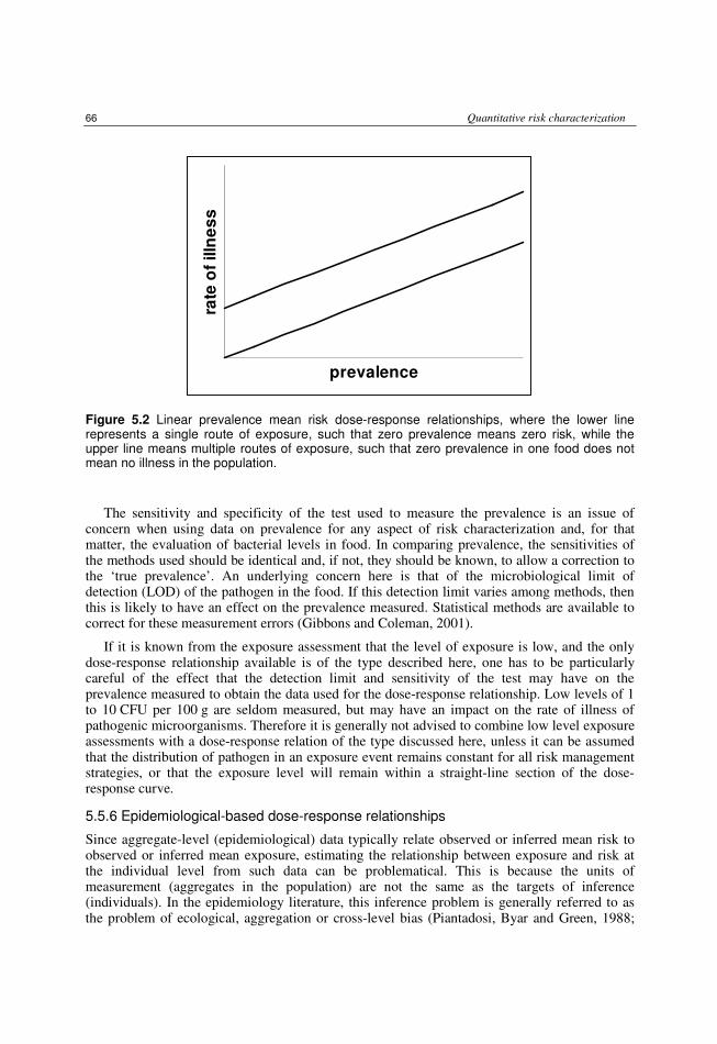
66 Quantitative risk characterization
prevalence
rate
of i
llnes
s
Figure 5.2 Linear prevalence mean risk dose-response relationships, where the lower line represents a single route of exposure, such that zero prevalence means zero risk, while the upper line means multiple routes of exposure, such that zero prevalence in one food does not mean no illness in the population.
The sensitivity and specificity of the test used to measure the prevalence is an issue of concern when using data on prevalence for any aspect of risk characterization and, for that matter, the evaluation of bacterial levels in food. In comparing prevalence, the sensitivities of the methods used should be identical and, if not, they should be known, to allow a correction to the ‘true prevalence’. An underlying concern here is that of the microbiological limit of detection (LOD) of the pathogen in the food. If this detection limit varies among methods, then this is likely to have an effect on the prevalence measured. Statistical methods are available to correct for these measurement errors (Gibbons and Coleman, 2001).
If it is known from the exposure assessment that the level of exposure is low, and the only dose-response relationship available is of the type described here, one has to be particularly careful of the effect that the detection limit and sensitivity of the test may have on the prevalence measured to obtain the data used for the dose-response relationship. Low levels of 1 to 10 CFU per 100 g are seldom measured, but may have an impact on the rate of illness of pathogenic microorganisms. Therefore it is generally not advised to combine low level exposure assessments with a dose-response relation of the type discussed here, unless it can be assumed that the distribution of pathogen in an exposure event remains constant for all risk management strategies, or that the exposure level will remain within a straight-line section of the dose-response curve.
5.5.6 Epidemiological-based dose-response relationships
Since aggregate-level (epidemiological) data typically relate observed or inferred mean risk to observed or inferred mean exposure, estimating the relationship between exposure and risk at the individual level from such data can be problematical. This is because the units of measurement (aggregates in the population) are not the same as the targets of inference (individuals). In the epidemiology literature, this inference problem is generally referred to as the problem of ecological, aggregation or cross-level bias (Piantadosi, Byar and Green, 1988;

Risk characterization of microbiological hazards in food 67
Greenland and Morgenstern, 1989; Richardson, Stucker and Hemon, 1987). Ecological bias includes the potential effect of confounders, but it is recognized that aggregation itself, in absence of any confounders, can bias aggregate-level relationships relative to underlying individual-level relationships. This is generally referred to as aggregation or cross-level bias.
There is no generally accepted ‘solution’ to this problem of bias in interpretation of aggregate-level data. However, choosing an appropriate definition of ‘mean’ risk or exposure, or both, for the groupings (e.g. geometric versus arithmetic mean) of the data used in hazard characterization may help to reduce the effects of bias to a practical level when the derived relationship is intended to represent risk versus dose at the individual level (Haas, 1996; Crump 1998; Guo et al., 1998). Alternative and more sophisticated approaches to reducing the effects of ecological bias exist (King, 1997) but such methods may not be applicable to microbiological risk assessment given the nature and extent of other biases that may be present.
The effects of cross-level bias are an issue of potential concern regardless of the form of the exposure assessment output, be it low-level, high-level or prevalence-based exposure. However, given the nature and extent of other uncertainties, the effect of cross-level bias may be particularly relevant when the dose response is integrated with an exposure assessment where exposures are quantitative at a high level.
5.5.7 Integration of variability and uncertainty
The way in which results from exposure assessment and hazard characterization are integrated will depend on the approach that has been taken to account for variability and uncertainty. The approach taken at each stage should be consistent so that, for example, if exposure has been stratified according to the susceptibility of different populations, there should be a dose-response model for each population. It is important to correctly match these model characteristics when combining results. For example, if variability between subpopulations has been accounted for, the probability distribution for exposure in each individual population should be propagated through the dose-response model for that population.
These ideas are illustrated in Figure 5.3. Here, it is assumed that exposure depends on season (A and B) and producer (1 and 2), leading to 4 different distributions of exposure (A1, A2, B1, B2). In addition, it is assumed that there are two subpopulations, each of which has its own dose-response curve. The figure shows that it is important to link the correct exposure model with the correct dose-response model if exposure and dose-response are stratified in this way.
The ideas of linkage are further illustrated in Figures 5.4 to 5.7, taking account of variability and uncertainty. In particular, they show results from example models in which stratification of the population and uncertainty have been incorporated to different degrees. In each case, the exposure assessment yields the probability that a randomly selected serving of the food product is contaminated with the microorganism and a probability distribution for the log number of organisms in such a serving. It has been assumed that any variability in contamination across, for example, seasons, areas of the country or food producers has been accounted for via averaging, and thus stratification is not required. The hazard characterization gives the dose-response model. It should be noted that the graphs showing the dose-response models are not probability or uncertainty distributions: they are mathematical functions. Finally, the risk characterization presents two measures of risk. The first measure is at the individual level and is given by the probability that a randomly selected individual becomes ill from consuming a serving of the food product. The second measure is at the population level, defined as the number of cases in the next year.

68 Quantitative risk characterization
Uncertainty is not included in the models shown in Figures 5.4 and 5.5. This results in point values for the probability of contamination and individual risk, single-dose-response models and single-probability distributions for the log number of organisms and population-level risk. If, for example, large samples were available, and thus randomness and differences between populations dominant, this approach would be appropriate. Alternatively, results like these would be obtained if the effect of uncertainty is to be investigated by changing the model parameters.
Second-order models are represented by Figures 5.6 and 5.7. This means that there is an uncertainty distribution for both the probability that a serving is contaminated and the individual risk (note the y-axis on each of these graphs – it shows confidence rather than probability). There is also uncertainty associated with the dose-response model and the probability distributions for the log numbers per serving and the population risk. This uncertainty is indicated by the multiple curves on each graph. This approach is appropriate if the uncertainty is large and can be explicitly separated from variability at all stages.
The difference in results when stratification of the population is included compared with not included can be seen by comparing Figures 5.4 and 5.5 (without uncertainty) and Figures 5.6 and 5.7 (with uncertainty). For the models in Figures 5.5 and 5.7, it has been assumed that there are differences in response between two subpopulations. This is indicated by the different dose-response models: subpopulation 1 is less susceptible than subpopulation 2 (although it assumed that both populations have the same level of exposure). The different dose-response models lead to different individual levels of risk, with a randomly selected individual from subpopulation 1 having a higher probability of illness than a randomly selected individual from subpopulation 2. The population-level risk aggregates the results from the two subpopulations to give the number of cases in the total population. If it can be assumed that there is no difference in response between subpopulations, then stratification would not be required (Figures 5.4 and 5.6).
The examples shown here can easily be extended to recognize, for example, variability across producers, across time or area (as shown in Figure 5.3). In addition, further estimates of risk could be derived.
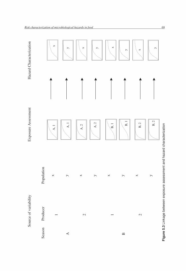
Fig
ure
5.3
Lin
kage b
etw
ee
n e
xpo
sure
asse
ssm
en
t an
d h
azard
ch
ara
cteri
zatio
n
Sea
son
Pro
du
cer
Pop
ula
tio
n
Sou
rce
of
var
iab
ilit
y
A B
1 2 1 2
x y x y x y x y
Exp
osu
re A
sses
smen
tH
azar
d C
har
acte
riza
tion
A, 1
A, 1
A,
2
A, 2
B,
1 B,
1
B, 2
B,
2
x
y x y x
y x
y
Risk characterization of microbiological hazards in food 69

70 Quantitative risk characterization
Figure 5.4. Risk characterization without stratification of the population and uncertainty not included
Exposure Assessment Hazard Characterization
Population
Risk CharacterisationPopulation
Individual risk
Population risk
Population
0
0.2
0.4
0.6
0.8
1
0 2 4 6 8 10
Log N per serving
Cu
mu
lati
ve
pro
ba
bil
ity
0
0.2
0.4
0.6
0.8
1
Serving contam inated Serving not contam inated
Pro
ba
bili
ty
0
0.2
0.4
0.6
0.8
1
1.2
0 2 4 6 8 10 12
Log Dose
Pro
ba
bili
ty o
f ill
ne
ss
0
0.2
0.4
0.6
0.8
1
Ill from a serving Not ill from a serving
Pro
ba
bil
ity
0
0.2
0.4
0.6
0.8
1
0 100 200 300 400 500
Number of cases in the next year
Cu
mu
lati
ve
pro
bab
ility

Exp
osu
re A
sses
smen
tH
aza
rd C
hara
cter
izati
on
Su
b-p
op
ula
tion
1S
ub
-po
pu
lati
on
2
Ris
k C
ha
ract
eris
ati
on
Su
b-p
op
ula
tio
n 1
Su
b-p
op
ula
tio
n 2
Ind
ivid
ual
risk
Po
pu
lati
on
ris
k
Su
b-p
op
ula
tio
n 1
Su
b-p
op
ula
tio
n 2
0
0.2
0.4
0.6
0.81
02
46
81
0
Lo
g N
pe
r s
erv
ing
Cumulative probability
0
0.2
0.4
0.6
0.81
02
46
81
0
Lo
g N
pe
r s
erv
ing
Cumulative probability
0
0.2
0.4
0.6
0.81
1.2
02
46
81
01
2
Lo
g D
os
e
Probability of illness
0
0.2
0.4
0.6
0.81
02
46
81
01
2
Lo
g D
os
e
Probability of illness
0
0.2
0.4
0.6
0.81
Se
rvin
g c
on
tam
ina
ted
Se
rvin
g n
ot
co
nta
min
ate
d
Probability
0
0.2
0.4
0.6
0.81
Se
rvin
g c
on
tam
ina
ted
Se
rvin
g n
ot
co
nta
min
ate
d
Probability
0
0.2
0.4
0.6
0.81
Ill f
rom
a s
erv
ing
No
t ill
fro
m a
se
rvin
g
Probability
0
0.2
0.4
0.6
0.81
Ill f
rom
a s
erv
ing
No
t ill
fro
m a
se
rvin
g
Probability
0
0.2
0.4
0.6
0.81
01
00
20
03
00
40
05
00
Nu
mb
er
of
ca
se
s i
n t
he
ne
xt
ye
ar
Cumulative probability
Fig
ure
5.5
. R
isk c
hara
cteri
zation
with s
tratificatio
n o
f th
e p
opu
lation
an
d u
nce
rta
inty
not
inclu
de
d.
Risk characterization of microbiological hazards in food 71

72 Quantitative risk characterization
Exposure Assessment Hazard Characterization
Population
Risk CharacterisationPopulation
Individual risk
Population risk
0
0.2
0.4
0.6
0.8
1
0 0.1 0.2 0.3
Probability serv ing contaminated
Cu
mu
lati
ve
co
nfi
de
nc
e
Population
0
0.2
0.4
0.6
0.8
1
0 2 4 6 8 10
Log N per serv ing
Cu
mu
lati
ve
pro
bab
ility
0
0.2
0.4
0.6
0.8
1
1.2
0 2 4 6 8 10 12
Log Dose
Pro
ba
bil
ity
of
illn
ess
0
0.2
0.4
0.6
0.8
1
0 0.002 0.004 0.006 0.008 0.01
Probability of illness from a serv ing
Cu
mu
lati
ve
co
nfi
de
nc
e
0
0.2
0.4
0.6
0.8
1
0 100 200 300 400 500
Numbe r of cases in the next year
Cu
mu
lati
ve
pro
bab
ilit
y
Figure 5.6 Risk characterization with no stratification of the population and uncertainty included

Ex
po
sure
Ass
essm
ent
Ha
zard
Ch
ara
cter
iza
tio
n
Su
b-p
op
ula
tio
n 1
Su
b-p
op
ula
tio
n 2
Ris
k C
ha
ract
eris
ati
on
Su
b-p
op
ula
tio
n 1
Su
b-p
op
ula
tio
n 2
Ind
ivid
ua
l ri
sk
Po
pu
lati
on
ris
k
0
0.2
0.4
0.6
0.81
00
.10
.20
.3
Pro
ba
bil
ity s
erv
ing
co
nta
min
ate
d
Cumulative confidence
Su
b-p
op
ula
tio
n 1
Su
b-p
op
ula
tio
n 2
0
0.2
0.4
0.6
0.81
00
.10
.20
.3
Pro
ba
bil
ity s
erv
ing
co
nta
min
ate
d
Cumulative confidence
0
0.2
0.4
0.6
0.81
02
46
81
0
Lo
g N
pe
r s
erv
ing
Cumulative probability
0
0.2
0.4
0.6
0.81
02
46
81
0
Lo
g N
pe
r s
erv
ing
Cumulative probability
0
0.2
0.4
0.6
0.81
1.2
02
46
81
01
2
Lo
g D
os
e
Probability of illness
0
0.2
0.4
0.6
0.81
02
46
81
01
2
Lo
g D
os
e
Probability of illness
0
0.2
0.4
0.6
0.81
00
.00
20
.00
40
.00
60
.00
80
.01
Pro
ba
bil
ity o
f il
lne
ss
fro
m a
se
rvin
g
Cumulative confidence
0
0.2
0.4
0.6
0.81
00
.02
0.0
40
.06
0.0
80
.1
Pro
ba
bil
ity
of
illn
es
s f
rom
a s
erv
ing
Cumulative confidence
0
0.2
0.4
0.6
0.81
01
00
20
03
00
40
05
00
Nu
mb
er
of
ca
se
s i
n t
he
ne
xt
ye
ar
Cumulative probability
Fig
ure
5.7
Ris
k c
hara
cte
riza
tion
with s
tra
tifica
tio
n o
f th
e p
op
ula
tio
n a
nd u
ncert
ain
ty inclu
ded
Risk characterization of microbiological hazards in food 73
74 Quantitative risk characterization
5.6 Examples of quantitative risk analysis
5.6.1 FSIS E. coli comparative risk assessment for intact (non-tenderized) and non-intact (tenderized) beef (USDA FSIS, 2002)
Mechanical tenderization performed using stainless steel blades or needles translocates pathogens from the surface of intact beef cuts to beneath the surface thereby potentially shielding those pathogens from the lethal effects of heat during cooking.
FSIS wished to estimate whether blade-tenderized steak posed a significantly greater risk than its equivalent non-tenderized steak. They created a quantitative simulation model that looked at the bacterial levels on the steaks, and the change in survival of bacteria due to the extra protection that was afforded by being embedded in the meat through the tenderizing process. They then estimated the bacterial load on steaks post-cooking, and used this concentration as input into a dose-response model to estimate risk. FSIS concluded:
“The probability of E. coli O157:H7 surviving typical cooking practices in either tenderized or not-tenderized steaks is minuscule … 0.000026 percent (i.e. 2.6 of every 10 million servings) of steaks that are not tenderized contain one or more bacteria. For tenderized steaks, 0.000037 percent (i.e. 3.7 of every 10 million servings) contain one or more bacteria. … Differences in bacterial dose after cooking attributable to tenderized versus not-tenderized steaks are minimal at most. [The model] shows a barely discernable difference at dose levels greater than 1 between tenderized and not-tenderized steaks. The expected illnesses per serving (IPSEV) for tenderized steaks is 1 illness per 14.2 million servings (7.0×10⁻⁸). For not-tenderized steaks the IPSEV is 1 illness per 15.9 million servings (6.3×10⁻⁸). What this means is that there will be seven additional illnesses due to tenderization for every billion steak servings (7.0×10⁻⁸ - 6.3x10⁻⁸)”
This was a comparative risk assessment so the model contained only the elements that were necessary to make the comparison. Thus, the model began with the distribution of bacteria on steak prior to tenderizing, and then looked at the difference in human health risk posed by the same steak under different processing, and did not need to consider any factors involved in the rearing and slaughtering of the animal.
5.6.2 FAO/WHO Listeria monocytogenes in ready-to-eat foods (FAO/WHO, 2004)
FAO/WHO convened a drafting group to address three questions relating to Listeria monocytogenes that were posed by the Codex Committee on Food Hygiene (CAC, 2000), namely:
• Estimate the risk of serious illness from L. monocytogenes in food when the number of organisms ranges from absence in 25 grams to 1000 colony forming units (CFU) per gram or millilitre, or does not exceed specified levels at the point of consumption.
• Estimate the risk of serious illness for consumers in different susceptible population groups (elderly, infants, pregnant women and immuno-compromised patients) relative to the general population.
• Estimate the risk of serious illness from L. monocytogenes in foods that support its growth and foods that do not support its growth at specific storage and shelf-life conditions.
The risk assessment did not need to complete a full farm-to-fork model to answer these questions. The questions are also not specific to a particular country or product, which would require defining the scope of the model. The team decided to focus on the level of Listeria
Risk characterization of microbiological hazards in food 75
monocytogenes at retail; model the growth and attenuation from retail to consumption; and use a fitted dose-response function to estimate the subsequent risk.
The team selected four ready-to-eat foods to be reasonably representative of the many different foods available. The quantitative analysis produced the results shown in Table 5.1.
Table 5.1 Estimated risk from Listeria monocytogenes as used in the FAO/WHO MRA.
Food Cases of listeriosis per 109 people per year
Cases of listeriosis per 109 servings
Milk 910 0.5
Ice cream 1.2 0.0014
Smoked fish 46 2.1
Fermented meats 0.066 0.00025
SOURCE: Adapted from Table 1 of FAO/WHO Listeria monocytogenes ready-to-eat risk assessment (FAO/WHO, 2004).
The risk assessment report provides a very detailed explanation of the important limitations of the quantitative analysis, and in particular the need to rely on mostly European quantitative data on contamination, and on multiple sources for prevalence estimates. Consumption data were mainly North American, and the dose-response relationship was derived from epidemiological data from the United States of America, which may not have the same exposure levels as the European data. Its summary response to the three Codex questions recognizes the caution that should be applied in interpreting the quantitative figures, by providing qualitative responses. For example (FAO/WHO, 2004):
“(T)he risk assessment demonstrates that the vast majority of cases of listeriosis result from the consumption of high numbers of Listeria, and foods where the level of the pathogen does not meet the current criteria, whatever they may be (0.04 or 100 CFU/g). The model also predicts that the consumption of low numbers of L. monocytogenes has a low probability of causing illness. Eliminating higher levels of L. monocytogenes at the time of consumption has a large impact on the number of predicted cases of illness.”
5.6.3 Shiga-toxin-producing E. coli O157 in steak tartare patties (Nauta et al., 2001)
In a risk assessment on Shiga-toxin-producing E. coli O157 in steak tartare patties, Nauta et al. (2001) simulated the exposure to the population in the Netherlands using a farm-to-fork Monte Carlo model. This risk assessment provided an example of integration of exposure assessment and hazard characterization with a low-level dose and an individual-level dose-response relation. The baseline model prediction of the exposure was characterized by a prevalence of 0.29% contaminated tartare patties and a mean number of 190 CFU per contaminated patty. The distribution of CFU in contaminated patties is summarized in Table 5.2. This distribution, when combined with consumption data on the probability of consumption of a steak tartare patty per person per day, results in an exposure assessment for the population in units of CFU per person per day.
The dose-response model developed for hazard characterization was based on a well documented outbreak in a primary school in Japan (Shinagawa, 1997). Data were fitted to an exponential model separately for children and adults, resulting in point estimates for the probability of infection by a single cell of r=0.0093 for children and r = 0.0051 for adults.

76 Quantitative risk characterization
Table 5.2 Distribution of exposure to STEC O157 in steak tartare patties.
CFU per exposure probability
1 63.9%
2–10 28.8%
11–100 6.3%
101–1000 0.9%
>1000 0.11%
Due to generally low levels of CFU per exposure, the exposure distribution was combined with the dose-response model in a Monte Carlo simulation by applying the single-hit model in the form 1-(1-r)n, with n a random sample from the exposure distribution. Risk characterization using this approach resulted in a predicted attack rate of 0.0015% infections per person per year in the Netherlands; that is, 2335 infections per 15.6 million people per year.
Note that in this example uncertainty is not quantified; only variability is incorporated.
5.6.4 FAO/WHO risk assessment of Vibrio vulnificus in raw oysters (FAO/WHO, 2005)
An FAO/WHO assessment of the risk of illness due to V. vulnificus in raw oysters was undertaken by adapting a risk model structure previously developed in the United States of America for V. parahaemolyticus (FAO/WHO, 2005),. This risk assessment provides an example of integration of exposure assessment and hazard characterization, when a dose-response estimated from aggregate-level data displays appreciable bias when interpreted as valid on the level of individual exposures. A principle objective in constructing the model for V. vulnificus was to investigate potential effectiveness of mitigations after development of a baseline model.
A dose-response relationship for V. vulnificus was obtained by fitting a parametric model (Beta-Poisson) to estimated population- or aggregate-level data on arithmetic mean risk versus arithmetic mean dose over groupings of the data defined by season and year. These estimated dose-response data were based on epidemiological surveillance of cases, consumption statistics and model-based estimates of V. vulnificus density. The resulting dose-response model fit was interpreted as an empirical fit. By construction, the result of integrating, or recombining, the derived dose response with the baseline exposures used to develop it should be equal, on average, to the population-level mean risks on which it was also based. This, however, was not the case when the estimated dose response was interpreted as applying at the level of individuals as well as on the level of the groupings from which it was derived: an apparent consequence of the effect of cross-level bias.
The magnitude of the difference between risk predictions obtained under these two alternative interpretations of the dose response is shown in Table 5.3. Assuming that the fitted population-level risk versus dose relationship applied at the individual level resulted in predictions of risk that were consistently lower (by up to 75%) than the epidemiological estimates of mean risks. The predictions of risk obtained based on an aggregate-level interpretation of the dose response were necessarily more consistent, on average, with the epidemiological estimates of mean risks used to obtain the dose-response fit. Consequently, this interpretation was used for risk characterization.
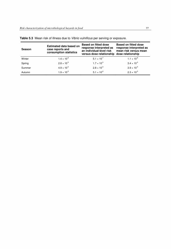
Risk characterization of microbiological hazards in food 77
Table 5.3 Mean risk of illness due to Vibrio vulnificus per serving or exposure.
Season Estimated data based on case reports and consumption statistics
Based on fitted dose response interpreted as an individual-level risk versus dose relationship
Based on fitted dose response interpreted as mean risk versus mean dose relationship
Winter 1.4 × 10⁻⁶ 5.1 × 10⁻⁷ 1.1 × 10⁻⁶
Spring 2.8 × 10⁻⁵ 1.7 × 10⁻⁵ 3.4 × 10⁻⁵
Summer 4.9 × 10⁻⁵ 2.8 × 10⁻⁵ 3.9 × 10⁻⁵
Autumn 1.9 × 10⁻⁵ 5.1 × 10⁻⁶ 2.3 × 10⁻⁵

6. Quality assurance
Risk characterization not only synthesizes the results of the previous parts of the risk assessment but also summarizes the overall findings and presents the strengths and limitations of the analysis to risk managers. The validity of the risk assessment is based on the soundness of the model structure, its input, the underlying assumptions and the interpretation of results. Therefore, quality assurance is a crucial element of risk characterization. Quality assurance can be achieved through a variety of methods. Data quality assurance is discussed in Section 6.1. Assessing the weight of evidence is discussed in Section 6.2. The sensitivity analysis is described in Section 6.3, while uncertainty analysis is addressed in Section 6.4. Model verification, anchoring and validation are addressed in Sections 6.5, 6.6 and 6.7, respectively. A specific method for model validation, involving comparison to epidemiological data, is discussed in Section 6.8. Model robustness and issues pertaining to model extrapolation are addressed in Section 6.9. The criteria for risk assessment credibility discussed in Section 6.10 include proper documentation of the analysis and peer review of the assessment. Public review is discussed in Section 8.5.
6.1 Data quality assurance
The results of sensitivity or uncertainty analysis are conditional on the data and other information used to develop the risk assessment model. Because it serves as the primary vehicle for communicating the risk assessment findings to risk managers, a risk characterization should briefly summarize the primary strengths and limitations of the data, methods, and analyses identified in the hazard identification, exposure assessment, and hazard characterization. Typically, these analyses require risk assessors to synthesize and draw inferences from disparate data sources not specifically or originally intended for use in risk assessment. In some cases, this requires the use of unconventional or non-routine methods that might be highlighted for particularly close scrutiny to ensure that they are reasonable and correctly applied. For relevant details, see the FAO/WHO hazard characterization and exposure assessment guidelines (FAO/WHO, 2003, 2008).
6.1.1 Data collection
Usually the suitable data for a microbiological risk assessment are sparse. In practice, assessors should initially collect all reasonably obtainable data consistent with the assessment objective, and subsequently investigate the quality of the different data sources. When collecting data for input distributions, several issues should be considered in order to evaluate data quality. The following considerations apply to empirical data and information elicited from experts.
Ideally, risk assessors would have access to raw, un-summarized data. With raw data (if consisting of sufficient observations), statistical methods such as Goodness-of-Fit tests are available to define a suitable parametric distribution describing the data. Alternatively, empirical distributions or non-parametric simulation methods can be used to characterize input distributions. Raw data, however, are frequently inaccessible. Often results are reported as aggregated summary statistics, such as the estimated mean, standard deviation or standard error of the mean. In order to develop a distribution from data summary statistics, it is necessary to obtain information on the assumed distribution of the underlying data, together with the sample size.

80 Quality assurance
It is useful to collect as much background information on the data sources as possible, such as the year of completion, country of origin, the type of sample, possible transformation of the data, methods of analysis, microbiological strain and population demographics. This information could be important with regard to treatment or use of the data or to support the decision on whether or not to include these data in the model. An example is given in Box 6.1.
Data for the specific microorganism under study may not always be available or of suitable quantity and quality (e.g. due to rare occurrence or imprecise collection methods). In that case, data from a surrogate microorganism can be used, provided that the surrogate behaves similarly under the process of interest (e.g. generic E. coli to estimate cross-contamination during slaughter procedures). In practice, data from different surrogate organisms could be used to model different steps in the same model, based on their availability and suitability. In some cases, sampled data with different units (e.g. absolute concentration or change in concentration) can be used in describing the same process, as the example below illustrates. Depending on how the data are used in the model (e.g. describing a change in concentration over a step or describing the concentration level, Figure 6.2), different parameters may be evaluated in a sensitivity analysis to ensure data quality objectives are satisfied.
Sensitivity analysis is a useful data quality assurance tool. Specific data sources and model inputs identified to have an important influence on model outputs warrant careful assessment. The available data may understate the true range of variability in a model input. In the example described above, the available data only covers two countries, and the variability may be greater than the empirical data alone suggest. Hence, techniques such as nominal range sensitivity analysis can be employed to evaluate the sensitivity of the model output to varying the model input across its entire range of plausible values. In other cases, the available data may not be considered representative of the population of interest. In such cases, the data may be excluded from the analysis or incorporated with appropriate adjustment. The bases for decisions regarding the treatment of non-representative data are context specific and need to be clearly articulated. For example, data from a particular source may be considered non-representative for the purposes of providing an estimate of central tendency (e.g. the mean) but useful for the purposes of characterizing the spread of an input distribution (e.g. plus or minus an order of magnitude).
Box 6.1 Example of a Danish risk assessment of Campylobacter jejuni in chicken. For the risk assessment, quantitative data were needed to describe the relative change in pathogen concentration over a given step in a poultry slaughterhouse (e.g. over the washing and chilling step, Figure 6.1). Because Danish data were unavailable, data from foreign studies were applied to assess the efficacy of the wash and chiller process in reducing the pathogen levels on chicken carcasses. Data for the microorganism of interest were available, but the data were obtained from different sample units (neck skin samples, whole carcass wash, and swab samples). This mix of sample types all reflected surface contamination of chicken carcasses. In synthesizing the data, it was assumed that the relative reduction in pathogen concentration over the process was independent of the type of surface measure. In Figure 6.2, the slopes reflect differences in log-concentration over the process. Since all the slopes appear to be similar, all data sets were used in describing the reduction over the ‘wash + chiller’ process. (Christensen et al., 2001).

Risk characterization of microbiological hazards in food 81
Figure 6.1 Illustration of a ‘black-box’ sub-model connecting two observed data sets (i.e. ‘anchor points’) over a process. The relative reduction of the Campylobacter load on chicken carcasses was assumed to be independent of where on the carcass the sample was taken. When data are given as log CFU values, this means that the relative change in concentration over the process (wash + chiller) is obtained by subtracting the concentrations before and after the process.
0
1
2
3
4
5
6
before
wash+chiller
after wash+chiller
Co
nce
ntr
atio
n o
f C
amp
ylo
bac
ter
Mead et al (1995)
Oosterrom et al (1983) Izat et al (1988)
Cason et al (1997)
Figure 6.2 The influence of a selected slaughterhouse process on the Campylobacter concentration on chicken carcasses. The change in pathogen concentrations before and after the process is represented by a line connecting data points originating from the same study.
wash & chiller process
Concentration (log 10 cfu/g skin) Concentration (log 10 cfu/g skin)
wash & chiller process
Concentration (log 10 cfu/g skin) Concentration (log 10 cfu/g skin)

82 Quality assurance
6.1.2 Sorting and selecting data sources
After collecting potentially suitable data sets, one should evaluate each of them critically and select the data that will provide the best possible model input for a specific purpose, such as describing the level of contamination, prevalence or changes over a process. Plotting the parameter of interest with the 95% confidence intervals provides a useful overview (see Figure 6.3).
Stud
ies
1.
2.
3.
4.
5.
6.
7.
8.
9.
10.
95 % confidence interval
Stud
ies
1.
2.
3.
4.
5.
6.
7.
8.
9.
10.
95 % confidence interval
1.
2.
3.
4.
5.
6.
7.
8.
9.
10.
95 % confidence interval
Figure 6.3 Example of an overview of data from different studies, with their 95% confidence intervals.
In selecting the suitable data sets for incorporation into the risk assessment, both subjective and analytical criteria may be applied. Subjective evaluation criteria may include the representativeness of the geographical and temporal properties of the candidate study. For example, if study no. 1 in Figure 6.3 is the only foreign study and it is significantly different from the rest (based on analytical criteria), this data set could be excluded. In contrast, if the 10 studies all originate from the same country, same year, etc., but are reported by different laboratories, the differences may be due to variability among the laboratories and the assessor might decide to incorporate all of the studies in the model.
6.2 Progression and weight of evidence
Whether an assessment is quantitative or qualitative, the public health risk posed by a micro-organism can be conceived at a basic level as the product of hazard, exposure and susceptible consumers (Figure 6.4).
If any one of the three elements of the epidemiological triangle equals zero, then there is no risk. A preliminary quality assurance step, therefore, is to evaluate whether a risk assessment
RISK
HAZARD
EXPOSURE HOST
Figure 6.4 Epidemiological Triangle.

Risk characterization of microbiological hazards in food 83
reflects this logical progression of threshold questions, to which the risk assessor could respond yes or no (perhaps with a qualifying level of confidence). If the response to a threshold question is ‘no’, then the analysis proceeds no further. At each threshold, the weight of evidence should be evaluated according to clearly specified, scientific criteria. As more criteria are satisfied, the weight of evidence indicates a more credible risk. Although there is a prima facie public health risk posed by several pathogens commonly associated with acute foodborne illnesses, in the future, risk assessors are likely to confront more cryptic and increasingly complex risk management questions, such as the risk posed by antibiotic-resistant microorganisms, the burden of chronic sequelae, the effect of specific growth-inhibiting food product formulations, and the susceptibility of individuals with underlying health problems. Some preliminary quality assurance guidance is provided here, therefore, in the anticipation that weight-of-evidence determinations will become increasingly prominent in risk assessments of microbiological pathogens in food.
6.3 Sensitivity analysis
Complex risk assessments may have many input and output variables that are linked by a system of equations or other model structures. Sensitivity analysis is a broad set of tools that can provide insights to risk assessors and risk managers about the relative importance of the components of a risk assessment to the risk management question. The plausibility of important components is essential to the overall quality of the risk assessment. Changes in important components also can be expressed in terms of the influence that these inputs have on the answers to risk-management questions.
A key criterion for sensitivity analysis is that it must be relevant to a decision. Sensitivity analysis evaluates the effect of changes in model input values and assumptions on the model output, and thus on decisions that would be based on the model output. It can be used during model development to evaluate and refine model performance and can play an important role in model verification and validation throughout the course of model development and refinement. Sensitivity analysis can also be used to provide insight into the robustness of model results when making decisions.
Sensitivity analysis can also be used as an aid in identifying important uncertainties for purposes of prioritizing additional data collection or research. For these purposes, value of information (VOI) analysis can complement sensitivity analysis methods, because the return to risk management decision-making on research and data collection expenditures depends on a variety of additional considerations (e.g. cost and time).
Microbiological risk assessment models typically have the following characteristics, which can pose substantial challenges to the application of sensitivity analysis methods:
• non-linearities;
• thresholds (e.g. below which there is no growth of a microbiological pathogen);
• discrete inputs (e.g. integer numbers of animals or herds; yes or no indicators of contamination);
• incorporation of measurement error;
• variation in the scale (units and range) and shape of distributions of model inputs; and
• temporal and spatial dimensions, including dynamics, seasonality or inter-annual variability.

84 Quality assurance
Ideally, a sensitivity analysis method should provide not just a rank ordering of key inputs, but also some discriminatory quantitative measure of sensitivity, such that it is possible to clearly distinguish the relative importance of different inputs. For example, are there groups of inputs among which several inputs are of comparable importance, and is there clearly a difference in importance between such groups? Statistical-based methods such as regression analysis or analysis of variance (ANOVA) produce quantitative indicators of the relative importance of different inputs. Moreover, techniques such as regression analysis also provide an indication of the statistical significance of differences in sensitivity among inputs, based upon confidence intervals for regression coefficients.
This section emphasizes sensitivity analysis in quantitative risk assessment models, although some of the techniques (e.g. exploratory methods) may apply to both quantitative and qualitative assessments.
6.3.1 Sensitivity analysis in qualitative risk assessment
In examining an association between an agent and a putative adverse health effect, widely accepted criteria (e.g. Hill’s Criteria) have been established for determining whether the evidence is weak, moderate or compelling (e.g. Tomatis, 1990). Narrative criteria may be inherently subjective, and therefore difficult to reproduce. To the extent that the criteria can be evaluated objectively, however, different assessors using the same information should be able to independently reproduce a determination of whether the criteria have been satisfied. For example, the weight of evidence for causality is stronger if detection of the association has been independently reported from multiple sources, if the strength of association is correlated with the level of exposure to the agent, or changes in the putative causative agent precede changes in the observed effect. Determining whether such criteria are satisfied is evidence-based. If the results of a qualitative assessment are invariant to an accumulation of evidence regarding an association or, alternatively, to contradictory evidence, then the assessment is insensitive to the established criteria for evaluating causality. In a qualitative hazard characterization, an assessment based solely on the criteria of acute health outcomes could be insensitive to information regarding known chronic sequelae. Alternatively, a qualitative hazard characterization may be highly sensitive to weak evidence regarding chronic sequelae associated with an opportunistic pathogen that rarely causes acute illness. If a qualitative assessment finds that a pathogen poses a negligible risk based on the assumption that the pathogen does not grow under certain environmental conditions, and new information indicates that the pathogen is capable of growing under these conditions, then the sensitivity of the findings of the risk assessment to this new information may depend on prespecified criteria, e.g. Have the results been independently reproduced? Have the methods been exposed to peer review? At a minimum, the scientific basis and criteria for characterization of a qualitative risk assessment needs to be sufficiently transparent to permit assessment of the impact of new information or plausible alternative assumptions on the findings.
6.3.2 Sensitivity analysis in quantitative risk assessment
There are several approaches to sensitivity analysis. Saltelli, Chan and Scott (2000) provide a thorough exploration of the topic, summarized below.
Exploratory methods
Exploratory methods for sensitivity analysis are typically applied in an ad hoc manner, but can be of central importance to the assessment of key sources of uncertainty in an analysis. Some
Risk characterization of microbiological hazards in food 85
key sources of uncertainty in an assessment include qualitative features, such as the conceptual representation of the system under study, structure of the model, level of detail of the model, validation, extrapolation, resolution, boundaries and scenarios. It is not uncommon, for example, for the uncertainty about the true model form to be of much greater importance than the uncertainty associated with any model input for a given statistical model. An assessment of sensitivity of an analysis to changes in assumptions would not be complete unless consideration was given as to whether the scenario underlying the analysis is well specified. Methods for dealing with uncertainty regarding qualitative features of the analysis typically involve comparison of results under different structural assumptions. For example, a method for assessing the importance of different exposure pathways is to estimate the exposure associated with each pathway and to determine whether total exposures are dominated by only a few critical pathways. Similarly, if there is uncertainty regarding model structure, a common approach is to compare predictions based upon different models, each of which may have a different theoretical and mathematical formulation.
Statistical methods
Examples of statistical sensitivity analysis methods (also referred to as variance-based methods) include regression analysis, ANOVA, response surface methods, Fourier amplitude sensitivity test (FAST), mutual information index (MII), and classification and regression trees (CART) (Frey and Patil, 2002). Most of these methods are applied in conjunction with or after a Monte Carlo analysis. Regression analysis, ANOVA, FAST and MII provide quantitative measures of the sensitivity for each input. Regression analysis requires the assumption of a model form.
Graphical methods
Graphical methods represent sensitivity typically in the form of graphs, such as scatter plots and spider plots. The results of other sensitivity analysis methods (e.g. rank order correlation) also may be summarized graphically (e.g. by tornado charts). These methods can be used as a screening method before further analysis of a model, or to represent complex dependencies between inputs and outputs (For example, see McCamly and Rudel, 1995). For example, complex dependencies could include thresholds or non-linearities that might not be appropriately captured by other techniques.
Evaluation of sensitivity analysis methods
Each sensitivity analysis method provides different information regarding sensitivities of the inputs such as the joint effect of inputs versus individual effects, small perturbations of inputs versus the effect of a range of variation, or apportionment of variance versus mutual information. Because agreement among multiple methods implies robust findings, two or more different types of sensitivity methods might be applied where practicable, in order to compare the results of each method and draw conclusions about the robustness of rank ordering of key inputs. Non-parametric methods (e.g. Spearman’s rank correlation) are applicable to monotonic, non-linear models. Vose (2000) recommends the use of spider plots to illustrate the effect of individual input variables on the uncertainty of the model output.
86 Quality assurance
6.4 Uncertainty analysis
Uncertainty analysis evaluates the range and likelihood of model predictions. In the context of quality assurance, uncertainty analysis is a useful tool for characterizing the precision of model predictions.
In combination with sensitivity analysis, uncertainty analysis can also be used to evaluate the importance of model input uncertainties in terms of their relative contributions to uncertainty in the model outputs (Morgan and Henrion, 1990). There are a variety of methods for estimating uncertainty in a model output based upon uncertainty in model inputs. The choice of method depends on what information is of most interest, the functional form of the model, and, to some extent, the number of inputs for which uncertainty is characterized.
Methods typically applied include Monte Carlo simulation for generating samples from distributions assigned to each input. Sensitivity analysis methods such as regression and ANOVA can be used in combination with Monte Carlo simulation to identify model inputs that contribute most to uncertainty in model predictions. Helton and Davis (2002) provide an extensive literature review of methods for sensitivity analysis used in combination with sampling methods.
6.5 Model verification
Model verification is achieved by auditing the model to ensure that it operates as intended by the developer(s). Model verification should precede model validation. This process includes validation of the software code used to implement the model. Verification requires thorough documentation and transparency in the data, methods, assumptions and tools used, so that the model is independently reproducible. A well organized model structure facilitates the verification audit.
There are several major elements in model verification:
• Assess the correctness of the model formulation. For example, are the analytical equations correctly derived and free of error?
• Is the computerized version of the analytical model correctly implemented?
• Are the inputs correctly specified?
• Do the units of measurement propagate correctly through the model?
• Is the model internally consistent? For example, if an assumption is made in one part of the model, is it consistently applied throughout the model? Is there consistency within the model between the intermediate outputs and inputs?
It may be difficult in some cases to quantitatively verify computer code, especially for large models that are developed in a short time. However, the verification of computer code will be facilitated if good software engineering practices are followed, including clear specification of databases, development of a software structure design prior to coding, version control, clear specification of interfaces between components of a model, and good communication among project teams when different individuals are developing different components of a model. Model documentation and peer review are critical aspects of the verification process.

Risk characterization of microbiological hazards in food 87
6.6 Model anchoring
Anchoring is a technique in which the model is adjusted or calibrated to be more compatible with observed data. For example, model parameters may be adjusted to achieve agreement between model predictions and observed data. Anchoring is a generally accepted practice in health risk assessment and environmental modelling, and has been employed in one fashion or another in risk assessments in the United States of America on Salmonella Enteritidis in eggs, Listeria monocytogenes in ready-to-eat foods, Escherichia coli O157:H7 in ground beef, and for an international risk assessment on Vibrio vulnificus in oysters (FAO/WHO, 2005). Data from outbreaks could be considered as the ultimate ‘anchor’ for dose-response models and are also an important way to validate risk assessments. There is a trade-off, however, because anchoring compromises the ability to validate the model output through comparison with the observed data in situations without sufficient data to support both. In general, anchoring approaches that weight model inputs in proportion to their likelihood in light of the observed data are superior to using simple adjustment factors or censoring input values that are incompatible with the observed data (National Academy of Sciences, 2002).
Whatever the anchoring approach, considerable care must be taken to ensure that the adjustment procedure is well reasoned and transparent. If the model is to be both anchored and validated (using a withheld portion of the independent data), then anchoring should precede model validation.
6.7 Model validation
A judgement needs to be made as to whether the risk assessment model response is reasonable. Stated less formally, model validation procedures are aimed at answering the following types of questions: (1) does the model make sense?; (2) does the model respond in an appropriate manner to changes in input assumptions; and (3) do predictions respond in an appropriate manner to changes in the structure of the analysis. This is also referred to by some as a ‘reality check’, ‘laugh test’ or ‘confidence building’.
Model validation is highly dependent on the risk-management question, and the degree of validation required should be proportionate to the stakes of the decision. FAO/WHO (2003) defines model validation as demonstrating the accuracy of the model for a specified use and refers to different aspects of model validation. Conceptual validation concerns the question of whether the model accurately represents the system under study. Validation of algorithms concerns the translation of model concepts into mathematical formulae. Validation of software code concerns the implementation of mathematical formulae in computer language (see Section 6.5 on model verification). Functional validation concerns checking the model with independently obtained observations. Even if independent data are unavailable, a portion of the data may be withheld during model development to permit assessment of the model using the withheld data. When few data are available, however, the loss of information for model development may outweigh the benefit of withholding data for model evaluation.
Close agreement between an initial risk-modelling effort and independent validation data would be fortuitous. Agreement between the model output and validation data may be coincidental, however, and would not necessarily indicate that all of the intermediate models components are accurate. Typically, model development and refinement is an iterative process. Whether model validation or anchoring is considered, the credibility of the model may be strengthened by having multiple points at which the model can be compared to observed data. In general, the scientific credibility of a model is strengthened if consistent results are derived

88 Quality assurance
from different relevant data sources (labs, regions) or types (observational or experimental), or a combination. The required degree of relevance and consistency is a context-specific judgement. The tolerance for inconsistent answers depends on what constitutes an ‘important’ difference with respect to changes in model results. In the risk assessment context, an important difference in model results is one that would significantly modify the risk management decision under the relevant decisional criteria.
There are situations in which it may be difficult or practically impossible to completely validate a model. For example, because risk assessment models are often attempting to predict low probability events, it can be difficult to obtain an independent data set of sufficient sample size to make statistically significant comparisons of predictions versus observations. However, even in such situations, it may be possible to validate components of the model. For example, it may be possible to validate portions of the model that deal with a particular exposure pathway by making measurements of contaminant levels in specific foods.
In many cases, there may be insufficient or no independent data with which to compare model predictions. In these situations, alternatives to validation include:
• screening procedures to identify the most important model inputs and pathways;
• sensitivity analysis to identify the most important inputs or groups of inputs;
• uncertainty analysis to evaluate the effect of uncertainty in model inputs with respect to predictions;
• comparison among predictions of different models; and
• evaluation of sensitivity of results to different assumptions regarding scenarios, model boundaries, model resolution and level of detail.
While none of these techniques provides a direct validation of the model, each of these techniques provides insight into the sensitivity of the model predictions to key assumptions regarding the analysis. The response of the predictions to these procedures can be evaluated with respect to prior expectations, comparison with analogous systems, and theoretical justifications.
6.8 Comparison with epidemiological data
In order to make a valid comparison with a foodborne pathogen risk estimate, at least three factors need to be considered in deriving an epidemiological estimate from human surveillance data (Powell, Ebel and Schlosser, 2001).
• Cluster-weighted rate of illness If the risk assessment estimates the incidence of illness at the national level, the epidemiological estimate will need to extrapolate the rate of illness beyond the surveillance area to permit comparison at the national level. In this case, the raw reported rate in each surveillance area may be weighted by the population of the region represented by the area (e.g. state population size) to obtain a weighted average rate of illness (e.g. cases per 100 000 in the national population). If multiple years of surveillance data are available, then the data can be used to characterize year-to-year variability in the rate of illness.
• Adjust surveillance data to account for under-reporting Estimating the actual incidence of illness requires adjustment for recognized sources of under-
Risk characterization of microbiological hazards in food 89
reporting in human surveillance data. For example, some ill persons do not seek medical care, physicians do not obtain stool specimens from all patients, laboratories do not culture all stool samples for the pathogen of concern, and some proportion of the lab results are false negatives. If estimates are available on the proportion of cases at each step in the reporting process, the negative binomial distribution can be used in sequential fashion to estimate the number of cases missed at each step. In some cases, the proportions may be dependent on the nature or severity of symptoms. For example, a person with bloody diarrhoea may be more likely to seek medical care than one with non-bloody diarrhoea. In this case, the proportion of cases with different levels of symptoms must be estimated prior to accounting for the number of cases missed at each step, and the adjusted symptom-specific estimates are summed to estimate the total number of cases. In general, the degree of under-reporting tends to be substantial. The degree of under-reporting also varies among countries and between regions within countries.
• Etiological fraction attributable to food product(s) The etiological fraction refers to the proportion of cases attributable to an exposure pathway or a specific food product. If the scope of the risk assessment is limited to a particular food product, then the proportion of cases due to other exposure pathways (e.g. other foods, drinking water) needs to be subtracted from the overall estimate of illness obtained from the human surveillance data. In general, empirical data on the etiological fraction are scarce. It may be possible, however, to specify a range of uncertainty on the basis of expert judgement.
If observed epidemiological data are used to generate the dose-response model or to anchor the model, then these data are unavailable for independent model validation. If sufficient epidemiological data are available, however, a portion of the data may be withheld for the purposes of model validation.
6.9 Extrapolation and robustness
Model robustness refers to the performance of the model when its assumptions are violated. In this context, assumptions include model form and model inputs. Extrapolating model results to other settings may involve many forms of extrapolation: from the present to the future, from one geographical region to another, from one microorganism to another, from animals to humans, from human clinical trial subjects to the general population, from one human population to another, from the available data to values beyond the observed range of the data, from controlled experimental settings to operational environments, and so on. Some extrapolations can be made with relative confidence, while others require a leap of faith. Some degree of extrapolation is inevitable if risk assessment attempts to inform risk-management decisions, since the demands of risk management tend to outstrip the supply of relevant science. The importance of various forms of extrapolation made in risk assessment needs to be considered and, to the extent feasible and relevant to the decision at hand, characterized in a clear manner, either quantitatively or qualitatively.
Extrapolation is explicit when the selected values of model inputs are outside the range of values used to calibrate or validate the model, or both. However, there can also be hidden extrapolation. A hidden extrapolation occurs for a combination of values of each model input such that these values are enclosed by ranges used for calibration and validation, but for which that specific combination was not included or approximated during calibration or validation. Thus, simple range checks on each input will not guarantee that a hidden extrapolation cannot occur. Hidden extrapolation would typically be more of a problem for a system in which there are highly sensitive interactions among inputs.

90 Quality assurance
A model that is calibrated to a narrow range of values for each input may not be robust when applied to sensitivity or uncertainty analysis. The use of ranges or distributions rather than point estimates could lead to hidden or explicit extrapolations of the model. In addition, situations can arise in which a joint set of model inputs are sampled in a Monte Carlo analysis for singularity points of a model, leading to problems such as division by zero or unbounded results. Such problems can often be traced to simplifying assumptions in model development, mis-specification of distributions for model inputs, or computer software limitations. Problems such as these can arise in practice, particularly when working with a model or computer code that someone else developed and for which documentation may be inadequate.
A model is considered to be robust if it responds in a reasonable manner to variation in input values, while at the same time not being easily subject to singularity points or other structural issues that lead to substantial magnification of errors in input values, whether because of uncertainty or user error. Moreover, a model that is based on sound theory might be used with more confidence compared with a purely empirical model that is essentially a curve fit to a calibration database. There is a distinction between the robustness of a risk assessment model and the robustness of a risk management decision. From an analytical perspective, a risk management decision is robust if the decision is beneficial over a reasonably wide range of possible future outcomes regarding uncertainties associated with the many factors that influence the decision. One such source of uncertainty would typically include the risk assessment model itself.
6.10 Credibility of the risk assessment
Documentation, validation, and review are necessary criteria for the credibility of a risk assessment. None of these criteria is sufficient by itself, however, as credibility depends on all three criteria being satisfied in a manner that is proportionate to the stakes of the decision.
6.10.1 Risk assessment documentation
At a minimum, risk assessment documentation must enable the analysis to be independently reproduced. The principle of transparency also requires that the source or basis for model inputs and assumptions be clearly stated (e.g. by references to scientific literature, evaluation criteria or expert judgement). The expectation for risk assessment documentation should be reasonable, however, because in some cases, assumptions may be based on common knowledge or generally accepted practices in the field. For example, the lognormal distribution is commonly assumed for modelling variables that are the product of several other variables. Because risk assessments are difficult to fully validate, and because such assessment are used to inform public decision-making at various levels, including local, national, and international, pertaining to public health, it is critically important that the information used for the assessment, including the model, be accessible for review by experts and the lay public. Ideally, subject to resource constraints, the following information should be included in documentation of a risk assessment:
• data or references to data sources;
• scenario, including the temporal and spatial aspects of the exposure scenarios, the specific hazards addressed, the specified pathogens included, exposed populations and exposure pathways;
• analytical model used for analysis, including the theoretical or empirical basis;

Risk characterization of microbiological hazards in food 91
• discussion and comparison of alternative model formulations, and justification for choices made regarding model structure;
• assumptions regarding values assigned to model inputs, including point-estimates, ranges and distributions;
• model verification, including assessment of results from sensitivity and uncertainty analysis;
• model anchoring (calibration);
• model validation; and
• computer implementation of the analytical model, including software design.
6.10.2 Peer review
FAO/WHO (2003) notes that the credibility of risk assessment results can be improved by the process used to develop the results. Peer and public review of risk assessment results are an essential part of the process, but each type of review generates distinct and sometimes conflicting demands that should be addressed on their own terms. There is also a distinction between the scientific credibility of a risk assessment and the credibility of risk management decisions. Public review is addressed in Section 8.5.
Morgan and Henrion (1990) identify exposure to peer review as a basic tenet of good policy analysis. The focus of a scientific peer review is highly dependent on the risk management question that the risk assessment is intended to inform. Without reference to a well-defined and specific risk management question, peer review of a risk assessment may fail to focus on the particular uncertainties that are most likely to influence the risk management decision. For example, if the risk management question is “What is the likelihood that a specific pathogen occurs in a particular food production process?” then data gaps and other uncertainties regarding post-production processes are irrelevant to the decision. Peer review comments regarding the scope of the risk assessment, while potentially useful for future risk assessments, are not relevant to the adequacy of the risk assessment under review to inform the risk management decision for which it was intended. If a risk assessment has multiple objectives, peer review may help to identify which objectives an assessment satisfies, since an assessment that is adequate to inform one decision may be insufficient to support another. For a complex risk assessment, a thorough review can be difficult and time consuming, even if the documentation is adequate. In the case of large, complex risk assessments, a thorough review may require a multidisciplinary team and a significant budget. Therefore, the substantive and procedural benefits of peer review should be balanced by time and resource considerations. The level and extent of review should be proportionate to the stakes of the decision, taking into consideration the need for immediate action in the event of bona fide public health emergencies.
7. Linking risk assessment and economic analysis
7.1 Introduction
Economic analysis is a powerful tool to support decision-making. It provides a common denominator for evaluating diverse outcomes, ranging from public health outcomes to trade impacts. With benefits and costs in the same (monetary) units the net benefits of alternative strategies to reduce risks can then be compared.
A risk assessment model is likely to compare scenarios with and without alternative interventions for a specific pathogen. The risk manager can compare the baseline human health risk with the changes in risk for each of the interventions. The problem is how to value the diverse range of human health outcomes ranging from mild illness to death.
Economic analysis permits changes in human health impact to be evaluated in monetary terms or healthy life-year equivalents, often expressed as QALYs or Disability-adjusted life years (DALYs) (see Section 7.2.1). Once the public health protection benefits have been estimated, changes in industry and government sector costs, in both the short and long term, can be estimated for each intervention under consideration. The same approach can also be used to prioritize food for a single pathogen or to prioritize pathogen+food combinations to be considered for action. This economic analysis can inform the risk manager about the size of the likely gains and losses by different groups for each intervention option. Those options with the largest net benefits are preferred, unless the risk manager has other important considerations that would make that option unacceptable, or that are not readily translated into economic values, e.g. for ethical or cultural reasons.
However, the linkage between risk assessment and economic analysis as a means of supporting decision-making in the area of food safety is a very new approach that is still in development. One example is an economic analysis of the impact of labelling eggs with the objective of changing consumer behaviour, following a positive evaluation of this intervention in a risk assessment of Salmonella Enteritidis in eggs (DHHS-FDA, 2000). As part of United States of America law, new or amended regulations that are ‘significant’, i.e. if they have an annual effect on the economy of US$ 100 million, adversely affect a sector of the economy in a material way, adversely affect competition or adversely affect jobs, must undergo a Preliminary Regulatory Impact Analysis (PRIA). In this case, the PRIA showed that the economic analysis calculated US$ 260 million of health benefits in the first year of introduction of the new rules, and US$ 260 million in health benefits thereafter, compared with a cost of US$ 56 million in the first year and US$ 10 million dollars in increased costs thereafter.
Methods of economic analysis that could be used for evaluating the costs and benefits of food safety and of different states of health are described in the following section, prior to discussion of their application in food safety risk assessment and management.

94 Linking risk assessment and economic analysis
7.2 Economic valuation issues
Economic value can be determined for most products and their attributes by examining prices in the marketplace. Although a market for food safety may emerge, a market price for food safety does not exist yet, or is at least not measured. Food is not marketed, nor prices differentiated, on the basis of ‘safe’, ‘less safe’ or ‘not safe’. In the absence of clear market prices for food safety, economists and other health researchers have developed a number of approaches for valuing the benefits of reductions in morbidity and premature death for foodborne pathogens.
7.2.1 Valuation of health outcomes
To evaluate the benefits of different risk management interventions in risk assessment, reduction in cases of illness (acute illnesses and their complications) needs to be estimated. While generally a low probability event, most foodborne illnesses can also cause some type of complication (see Appendix 1; Foegeding and Roberts, 1994). It is useful to organize the medical data into a disease outcome tree (see Appendix Figure A1) to recognize and document the full range of acute illnesses and longer-term complications. Because the range of health outcomes is so broad, a simple outcome ranking, such as deaths, will leave out many other health outcomes. As a result it is difficult to describe and evaluate the full costs of the risk management strategies and to prioritize spending alternatives.
To establish a basis for comparing diverse health risks and for ranking policy alternatives, analysts must translate diverse outcomes into a common unit of analysis. Economists have played a major role in establishing a common unit of analysis for risk ranking and cost-benefit analysis. The Cost-of-illness (COI) and Willingness-to-pay (WTP) methods convert diverse outcomes to monetary units, and the QALY approach converts diverse outcomes to healthy-time equivalencies (Kuchler and Golan, 1999; Golan et al., 2003; Haddix et al., 1996; Tolley, Kenkel and Fabian, 1994).
To illustrate the complex sequence of events that can occur over one’s lifetime after an occurrence of foodborne illness (FBI), consider Figure 7.1, where the linkage between arthritis and exposure to foodborne pathogens is shown (Raybourne et al., 2003). At the first node of the tree is the estimate of the probability that a person exposed to a foodborne pathogen develops reactive arthritis. At the second node, either full recovery or the possible progression to ongoing arthritis is estimated. The final node characterizes the consequences of lifetime arthritis into: mild or intermittent joint pain; severe/chronic joint pain; or sacroiliitis/spondylitis (involving spine).

Risk characterization of microbiological hazards in food 95
Figure 7.1 Disease outcome tree of Arthropathies (Raybourne et al., 2003). The values shown are estimates of the mean proportion of cases in each category. Values shown in parentheses indicate the range of those estimates.
Cost-of-illness method
The COI method estimates the dollars spent on medical expenditures and the value of the productivity of the patient foregone as a result of foodborne illnesses, complications and deaths. The value of productivity is a notional value, e.g. based on average adult wage. The strength of the COI approach is the use of money as the common unit of measurement to provide a full ranking of policy options and a context for determining social desirability. The COI method translates health outcomes into monetary equivalents that can be added and permit analysts to rank different health outcomes. The net benefits of different policy options can be estimated by comparing, for each policy option, the change in public health protection benefits with the change in costs to the government, industry and consumers. If the net benefits of a programme exceed the estimated net costs, the programme is considered worthwhile in economic terms. Examples of application of the COI method for food safety include Roberts and Marks (1995) and Buzby et al. (1996).
Willingness-to-pay method
The WTP method involves solicitation of stakeholders about the maximum amount they are willing to pay for a specified theoretical service or good, e.g. to be guaranteed that a particular food would not cause them illness. This approach is the most consistent with economic theory. The WTP method for estimating the benefits of public health programmes rests on the observation that individuals can and do make trade-offs between health and other consumption goods and services. Individuals routinely and voluntarily accept many small risks in exchange for finite benefits. Some risks rank quite low when preferences are considered. For example, skiing carries a risk of injury and death, but very few skiers would welcome a government programme that banned skiing on the basis of risk. Similarly, some consumers prefer the taste and texture of rare hamburgers and are willing to assume some risk. There are profound differences in the way that individuals value reductions in different risks. The WTP method
Disease Outcome Tree of Arthropathies*
Acute FBI
Full recovery
Reactivearthritis
Progressive/recurrent arthritis
Sacroiliitis/Spondylitis
Full recovery
Severe/chronic joint pain
��������
������� � � ���
�������
���������
�����������
�����������
Mild or intermittentjoint pain
����������
���
����
���
���
���
���
*Following Exposure to Bacterial Foodborne Pathogens
96 Linking risk assessment and economic analysis
provides a means of ranking diverse risks, not just by the size of the risk, but also by how concerned stakeholders are about the risk. WTP estimates what risk reduction is worth to individuals whose health might benefit, provided they understand the full consequences of exposure to the foodborne pathogen being evaluated. This technique is beginning to be applied to foodborne disease risks (e.g. Golan and Kuchler, 1999; Brown, Oranfield and Henson, 2005).
Disability-adjusted life years
Some analysts or policy-makers prefer not to assign monetary values to human illness or death (Haddix et al., 1996). To avoid using money as a unit of account, one of the most popular methods is to construct a health index that accounts for changes in both length and quality of life. These may be surrogates for economic measures.
The DALY is based on the amount of ‘life quality’ lost, multiplied by the duration of that loss of life quality. For example, a DALY related to diarrhoea might be estimated as 50% disability (or 50% loss of life quality lost) for three to four days (equal to 1/100th of a year. Thus, the DALY is 0.5 times 0.01 = 0.005. For a foodborne illness leading to the premature death (100% loss of life quality) of a 35-year-old adult, the duration can be estimated as the number of years that the person might have been expected to still live (e.g. 40 years). Thus, the DALY in this case is 35. In a study of Shiga-toxin-producing Escherichia coli O157 in the Netherlands, acute gastroenteritis was estimated to be 6% of the total disease burden. The major disease burden (94%), despite there being far fewer cases, was associated with deaths from haemolytic uraemic syndrome and from the few cases that develop end-stage renal disease (Havelaar et al., 2003), a chronic and debilitating disease. The QALY concept is analogous, but measures the increase in quality of life, and its duration, as a result of an actual or putative intervention.
Because DALYs and QALYs provide a common unit of measure for different health outcomes, they provide a means for ranking and prioritizing funding allocation across diverse types of programmes, such as nutrition and dialysis programmes. All things equal, those programmes with the highest QALY per monetary unit should be funded before those with lower DALY per monetary unit. However, DALYs do not produce a net benefit measure. They do not provide a framework for evaluating the worth of a programme, i.e. how much money should be spent per QALY, nor would they be expected to equate naturally to health-care costs.
7.2.2 Valuation of non-health outcomes
In the context of international trade in food, microbiological food risk assessment focuses only on food safety as it relates to public health. Within nations, however, the introduction of new regulations often needs to demonstrate net benefits from the proposed regulations compared with the costs of their implementation. As such, in some risk assessments, non-health benefits, such as maintenance of access to export markets that are attributable to safe food and a strong food safety system, may also be important (Golan et al., 2003; Buzby and Roberts, 1997), and methods for their estimation are considered briefly here. In principle, market prices are available to estimate all non-health outcomes. However, the linkages to food safety risks can be difficult to quantify in advance. The economic consequences of BSE on British beef sales and exports, in which market losses have been extensive, is such an example.

Risk characterization of microbiological hazards in food 97
Value of reductions in market risks
Food safety concerns may trigger market fluctuations that are only loosely related to the real value of health risks. Hazards that have a very low ranking in terms of health risk can trigger market reactions that rank high in terms of economic impact. The global nature of food trade has the potential to amplify food safety scares. In these cases, the measure of the value of a food safety system should include its ability to reduce disruptions in domestic and international markets and in the economic losses these disruptions entail.
Value of access to foreign markets
A strong food safety system may also reap benefits in terms of access to foreign markets (Spriggs and Isaac, 2001; Roberts et al., 1997; Krissoff, Bohman and Caswell, 2002; Kaelin and Cowx, 2002). Many countries limit food imports to those countries with comparable or more stringent food safety systems. For many food producers, access to foreign markets is vital to the success of their business. For producers in these exporting countries, the value of a strong food safety system goes beyond the value of reducing domestic public health risks associated with foodborne pathogens
For example, a series of bans were imposed on fish exports from Uganda because of Salmonella and Cholera contamination and toxic levels of pesticides. From 1996 to 1999, an estimated 10 000 fisherfolk lost their jobs (Nasinyama, pers. comm., 2002). The economic loss to Uganda has been estimated at US$ 100 million. In 2000, the European Union lifted the ban on imports of fish. In 2001 Uganda was placed on the list of countries for export without restriction. Today, fish almost surpass coffee as Uganda's number one export (Kaelin and Cowx, 2002)
Value of consumer confidence and tourism lost due to unsafe food
A strong food safety system builds consumer confidence and can lend credibility to government programmes. Consumers’ confidence in the food safety system makes them less susceptible to passing food scares and limits market volatility. Following the salmonellosis and BSE crises in the United Kingdom, for example, consumers became concerned about their food regulatory system, which ultimately led to the creation of a new food standards agency. Additionally, if a country’s food supply is not considered safe, some tourists will decide not to visit. This will have wide impacts on a variety of businesses, including hotels, restaurants, transportation, crafts and many other local industries.
7.3 Integrating economics into risk assessments to aid decision-making
The outcome of a quantitative risk assessment will generally provide an estimate of the baseline human health risks. Usually, quantitative risk assessments give complete probability distributions rather than just point estimates of population risk. An example of incorporating both means and range for estimated health outcomes is shown in Figure 7.1, the disease outcome tree for arthritis after exposure to a foodborne pathogen. The mean and range can become the basis for developing a distribution of this health outcome. The economic costs for the baseline risk can be evaluated using one of the three techniques discussed (COI, WTP, QALY).
There are two basic methods for evaluating the benefits and costs of proposed changes to policy or regulations:

98 Linking risk assessment and economic analysis
• Cost–benefit analysis is most appropriate for human health risks evaluated using the COI or WTP approaches.
• Cost-effectiveness analysis is most appropriate for human health risks evaluated using the QALY approach.
The nature of each policy decision needs to be clearly understood to allow the identification of those who benefit and those who are disadvantaged by that policy (see Appendix Table A2)(Buzby and Roberts, 1997). In particular, it is important to ensure that benefits and disadvantages accrue fairly, e.g. that one group does not benefit at the expense of another being exposed to increased risk. The anticipated economic costs of the public health intervention (e.g. requiring changes in the behaviour of industry, government and possibly consumers) can then be compared with the economic evaluation of improvements in health outcomes.
7.3.1 Cost–benefit analysis
Cost–benefit analysis is a useful tool to evaluate the impact on society of alternative food safety interventions. The benefits of reduced risk are primarily the improvement in public health, although other impacts may be important in specific cases (such as trade or tourism). All benefits are estimated in monetary units. The improvements in public health are estimated using either the COI or WTP technique discussed above. The benefits are then compared with the costs of the intervention. Costs are also estimated in monetary units and can include changes in industry, government and consumer behaviour (see Appendix Table A2). For example, if the intervention is to put information on food labels asking consumers to change their kitchen practices, the value of the increased time involved can be estimated as a cost. Some technical finance issues in the cost–benefit analysis include deciding on the time horizon and the discount rate (Dinwiddy and Teal, 1996; Laylard and Glaister, 1996). The net benefits from alternative food safety interventions can then be compared. Those with the highest net benefits are preferred, although the decision-maker may have other considerations to take into account.
An analysis of the United States Department of Agriculture Pathogen Reduction/Hazard Analysis at Critical Control Points (PR/HACCP) rule for raw meat and poultry (Crutchfield et al., 1997) demonstrated the use of cost–benefit analysis. The public health benefits were predicted to derive from preventing diseases caused by four foodborne pathogens. Using the most conservative assumptions, the PR/HACCP was estimated to provide net benefits of US$ 7 billion or more over a 20-year period. When the analysis assumed higher rates of pathogen control and lower interest rates, the present value of the net benefits provided by PR/HACCP was US$ 42 billion (Table 7.1).
7.3.2 Cost effectiveness analysis
Cost-effectiveness analysis is often used by health economists to evaluate alternate methods of achieving a specific public health goal, such as reducing the number of deaths. The number of deaths can either be assessed directly or QALYs can be used to assess the net improvement in all health-related quality of life changes over the baseline due to a food safety intervention. The change in QALYs is then compared to the net costs. Costs evaluated include medical costs and lost productivity. The decision criterion is the cost-effectiveness ratio, where the gain in QALYs (or number of deaths) is the numerator and the net costs are the denominator. Those with the highest ratio are preferred.
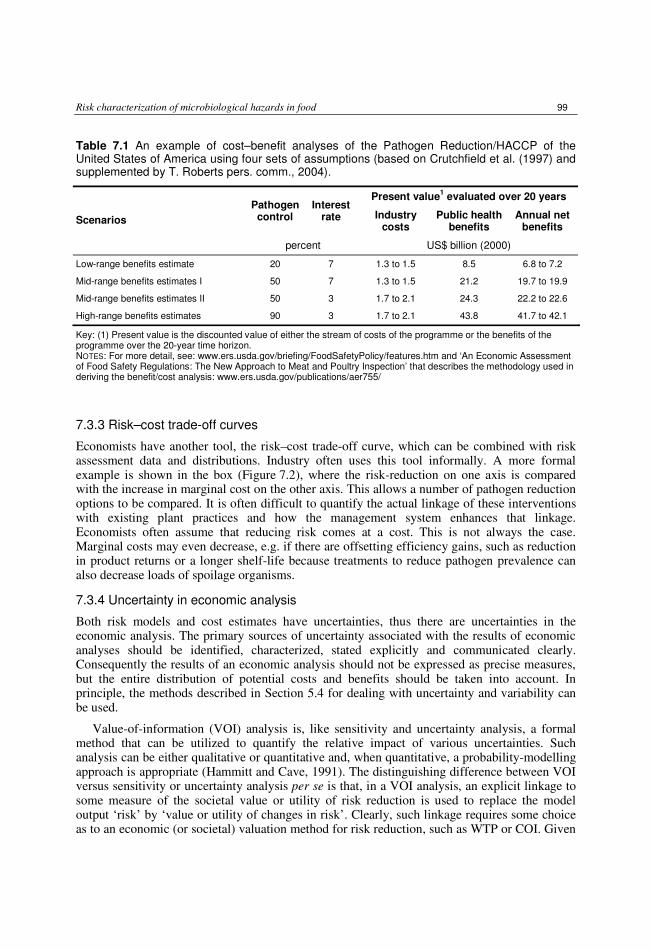
Risk characterization of microbiological hazards in food 99
Table 7.1 An example of cost–benefit analyses of the Pathogen Reduction/HACCP of the United States of America using four sets of assumptions (based on Crutchfield et al. (1997) and supplemented by T. Roberts pers. comm., 2004).
Present value1 evaluated over 20 years Pathogen
control Interest
rate Industry costs
Public health benefits
Annual net benefits
Scenarios
percent US$ billion (2000)
Low-range benefits estimate 20 7 1.3 to 1.5 8.5 6.8 to 7.2
Mid-range benefits estimates I 50 7 1.3 to 1.5 21.2 19.7 to 19.9
Mid-range benefits estimates II 50 3 1.7 to 2.1 24.3 22.2 to 22.6
High-range benefits estimates 90 3 1.7 to 2.1 43.8 41.7 to 42.1
Key: (1) Present value is the discounted value of either the stream of costs of the programme or the benefits of the programme over the 20-year time horizon. NOTES: For more detail, see: www.ers.usda.gov/briefing/FoodSafetyPolicy/features.htm and ‘An Economic Assessment of Food Safety Regulations: The New Approach to Meat and Poultry Inspection’ that describes the methodology used in deriving the benefit/cost analysis: www.ers.usda.gov/publications/aer755/
7.3.3 Risk–cost trade-off curves
Economists have another tool, the risk–cost trade-off curve, which can be combined with risk assessment data and distributions. Industry often uses this tool informally. A more formal example is shown in the box (Figure 7.2), where the risk-reduction on one axis is compared with the increase in marginal cost on the other axis. This allows a number of pathogen reduction options to be compared. It is often difficult to quantify the actual linkage of these interventions with existing plant practices and how the management system enhances that linkage. Economists often assume that reducing risk comes at a cost. This is not always the case. Marginal costs may even decrease, e.g. if there are offsetting efficiency gains, such as reduction in product returns or a longer shelf-life because treatments to reduce pathogen prevalence can also decrease loads of spoilage organisms.
7.3.4 Uncertainty in economic analysis
Both risk models and cost estimates have uncertainties, thus there are uncertainties in the economic analysis. The primary sources of uncertainty associated with the results of economic analyses should be identified, characterized, stated explicitly and communicated clearly. Consequently the results of an economic analysis should not be expressed as precise measures, but the entire distribution of potential costs and benefits should be taken into account. In principle, the methods described in Section 5.4 for dealing with uncertainty and variability can be used.
Value-of-information (VOI) analysis is, like sensitivity and uncertainty analysis, a formal method that can be utilized to quantify the relative impact of various uncertainties. Such analysis can be either qualitative or quantitative and, when quantitative, a probability-modelling approach is appropriate (Hammitt and Cave, 1991). The distinguishing difference between VOI versus sensitivity or uncertainty analysis per se is that, in a VOI analysis, an explicit linkage to some measure of the societal value or utility of risk reduction is used to replace the model output ‘risk’ by ‘value or utility of changes in risk’. Clearly, such linkage requires some choice as to an economic (or societal) valuation method for risk reduction, such as WTP or COI. Given
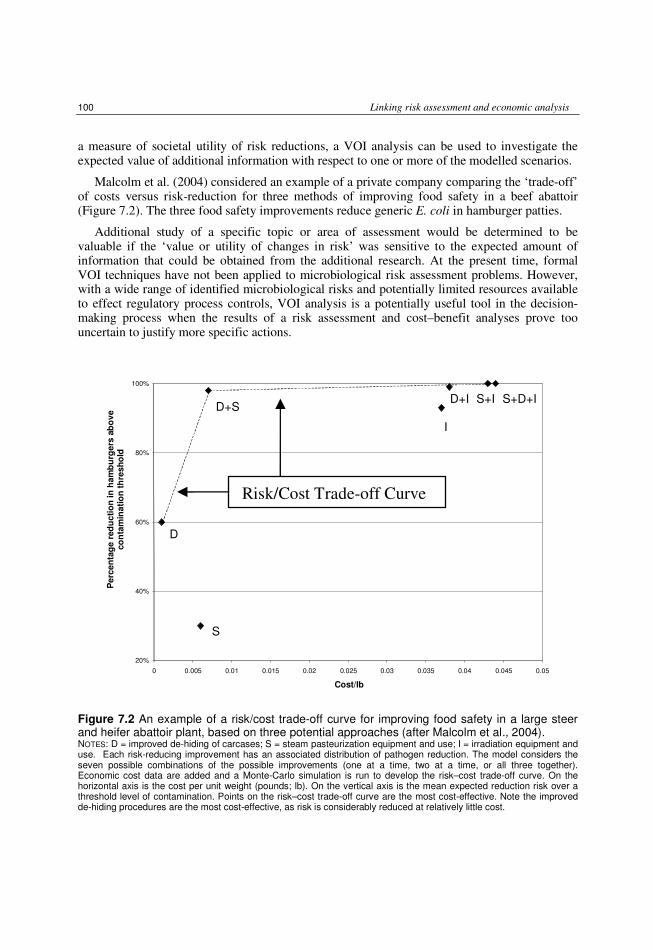
100 Linking risk assessment and economic analysis
20%
40%
60%
80%
100%
0 0.005 0.01 0.015 0.02 0.025 0.03 0.035 0.04 0.045 0.05 Cost/lb
Per
cen
tag
e re
du
ctio
n in
ham
bu
rger
s ab
ove
co
nta
min
atio
n t
hre
sho
ld
I S+I D+I
D+S
D
S
S+D+I
Risk/Cost Trade-off Curve
a measure of societal utility of risk reductions, a VOI analysis can be used to investigate the expected value of additional information with respect to one or more of the modelled scenarios.
Malcolm et al. (2004) considered an example of a private company comparing the ‘trade-off’ of costs versus risk-reduction for three methods of improving food safety in a beef abattoir (Figure 7.2). The three food safety improvements reduce generic E. coli in hamburger patties.
Additional study of a specific topic or area of assessment would be determined to be valuable if the ‘value or utility of changes in risk’ was sensitive to the expected amount of information that could be obtained from the additional research. At the present time, formal VOI techniques have not been applied to microbiological risk assessment problems. However, with a wide range of identified microbiological risks and potentially limited resources available to effect regulatory process controls, VOI analysis is a potentially useful tool in the decision-making process when the results of a risk assessment and cost–benefit analyses prove too uncertain to justify more specific actions.
Figure 7.2 An example of a risk/cost trade-off curve for improving food safety in a large steer and heifer abattoir plant, based on three potential approaches (after Malcolm et al., 2004). NOTES: D = improved de-hiding of carcases; S = steam pasteurization equipment and use; I = irradiation equipment and use. Each risk-reducing improvement has an associated distribution of pathogen reduction. The model considers the seven possible combinations of the possible improvements (one at a time, two at a time, or all three together). Economic cost data are added and a Monte-Carlo simulation is run to develop the risk–cost trade-off curve. On the horizontal axis is the cost per unit weight (pounds; lb). On the vertical axis is the mean expected reduction risk over a threshold level of contamination. Points on the risk–cost trade-off curve are the most cost-effective. Note the improved de-hiding procedures are the most cost-effective, as risk is considerably reduced at relatively little cost.

8. Risk communication aspects of risk characterization
8.1 Introduction
The various purposes of risk communication are outlined in The application of risk communication to food standards and safety matters (FAO/WHO, 1988).
Risk communication is defined in the Codex Procedure Manual (CAC, 2001) as:
The interactive exchange of information and opinions throughout the risk analysis process concerning hazards and risks, risk-related factors and risk perceptions, among risk assessors, risk managers, consumers, industry, the academic community and other interested parties, including the explanation of risk assessment findings and the basis of risk management decisions.
It is an integral and ongoing part of the risk analysis exercise, and ideally all stakeholder groups should be involved from the start. Risk communication makes stakeholders aware of the process at each stage of the MRA. This helps to ensure that the logic, outcomes, significance, and limitations of the MRA are clearly understood by all the stakeholders. Information may be available from the stakeholder. Industry stakeholders may, for example have unpublished data crucial to the risk assessors, which may be an essential part of the data needed for the risk assessment. There is also information that is typically presented to the stakeholders (both industry and consumers), as an integral part of the risk analysis process.
The identification of particular interest groups and their representatives should comprise a part of an overall risk communication strategy. This risk communication strategy should be discussed and agreed upon between risk assessors and managers early in the process to ensure two-way communication. This strategy should also cover who should present information to the public, and the manner in which it will be done.
• The risk communicators will need to identify the risk communication needs and specific strategy for each unique audience. An analysis of the level of awareness and knowledge of the issues for each audience as well as the best method for conveying information to them is critical in preparing risk communication messages, and to determine the appropriate channels of communications. Once audiences have been identified, the next step is to determine strategies for communicating that include both outward communications (messages, provision of information) and inward communication (listening to audience needs, gathering of information). It is important that the communication messages meet the specific needs of the various audiences.
• Some stakeholder groupings are relatively easily identified. In foodborne risk issues, these include such groups as risk managers and regulators, the general public, data holders, scientists, the media, consumer and industry representatives, and public health professionals. Audiences may also include consumers, especially those consumers at high risk for foodborne illness, such as the elderly, pregnant women, young children and people with weakened immune systems. As the whole population are stakeholders in food safety issues, in theory they could be involved in this information exchange. However, this would be very difficult in practice, and many individuals may be completely uninterested in taking an active part.
102 Risk communication aspects of risk characterization
Risk assessors and managers will need to inform stakeholders of the intention to perform a risk analysis at the start of the project. At this stage, communication with stakeholders is an important opportunity to develop trust, political and scientific support for the MRA, as well as a data gathering exercise.
8.1.1 Information to share with stakeholders
In food safety issues, there is rarely a valid reason why the public cannot have access to all the information used in an MRA, the full MRA report, and a full report of the considerations and (apart from specific issues of commercial confidentiality) the reasoning by which the risk managers reached their decisions. Where it is necessary to maintain commercial confidentiality, sensitive information can usually be presented as part of an overall summary. Specific topics that should be included in the reports to stakeholders include:
• Information on the risk itself, including the nature of the hazards; the estimated magnitude and severity of the risk; the method used to estimate magnitude and severity; information on trends over time; and differences in population susceptibility or exposure strata.
• Information on the uncertainties in the assessment, including input (data) uncertainties; output (estimate) uncertainties; and the assumptions used.
• Risk management considerations and options, such as information received, including stakeholder concerns; actions proposed or selected (dependant upon stage of communication process); reasons or justification for those actions; expected effects; and intended follow-up, monitoring and review activities.
When technical reports are provided to the stakeholders, it is essential that information is also provided in a way that is useful and comprehensible to those receiving it. Specific suggestions as to how information can be effectively presented are discussed below.
8.1.2 Major scientific issues in risk communication
Communicating scientific information is challenging, especially when there is a great deal of uncertainty. For fear of being misunderstood or misinterpreted, scientists and risk managers may be reluctant to communicate technical scientific information when there are significant uncertainties and differences of opinion between experts. For example, this may have been the case in regard to risks associated with bovine spongiform encephalopathy (BSE) in the UK (Chartier and Gabler, 2001).
Although in the past the public perceived scientific information as authoritative, this attitude has changed with respect to risks associated with food, and the public has become increasingly critical about estimates of risk. In addition, lack of understanding of mathematical probability and the enhanced profile of uncertainty associated with MRA are two factors that make public risk communication particularly difficult. Message framing (i.e. the way message is presented) is crucial in these circumstances.
8.2 Interaction between risk managers and risk assessors
From the viewpoint of the risk assessor, the risk manager is a special category of stakeholder, with specific additional communication requirements. As presented in the FAO/WHO report on Principles and guidelines for incorporating microbiological MRA in the development of food safety standards, guidelines and related texts (FAO/WHO, 2002), the interaction between risk assessors and risk managers should be ongoing throughout the Risk Analysis procedure. Risk

Risk characterization of microbiological hazards in food 103
communication aspects relevant to the various stages of the risk analysis procedure are highlighted below.
8.2.1 Planning and commissioning an MRA
Once the risk manager has decided to commission an MRA and selected the risk assessment provider, the planning and contracting of the work needs to take place. The planning and commissioning of the MRA procedure is probably one of the most important steps, in order to ensure the quality of the whole process, effective working relationships, and the appropriate outcomes from the MRA. Close communication between risk assessors and risk managers on the issues at this stage is crucial, and discussion should include the following:
(i) Scientific issues concerning the MRA.
• Background information, including provision of a Risk Profile.
• Initial risk management questions.
• The purpose and scope of the MRA.
• Expected outcomes of the MRA.
• The required form of the risk estimate (i.e. risk characterization measures and units).
• How it is intended that the outcome of MRA will be used in the risk management process.
• Criteria for validating the risk model and outcomes.
• Criteria to determine scientific and technical adequacy of the MRA.
• Consideration of the probable data needs.
(ii) Practical issues
• Basic and additional resources likely to be needed.
• Timelines and milestones.
• Frequency and timing of the interaction between the risk assessor and the risk manager.
• Communication strategy.
It is extremely helpful to widely publicize the intended method of assessment, and this should be done at the earliest possible opportunity (including any indications of the format and type of model most likely to be used), together with an expression of flexibility in the eventuality of any new information or ideas. The commissioning of the MRA should preferably be settled in a written contract between risk managers and risk assessors, with a clause indicating that the contract will be reviewed regularly as new information comes to light, to ensure milestones and outputs are still reasonable and appropriate.
8.2.2 During the MRA
Knowledge about data availability and understanding of the problem will usually greatly improve during the development of the MRA. The initial questions asked by the risk managers often need to be modified during the early stages of the MRA, as information and data limitations become clear. Thus decisions on the final scope of the assessment and questions to

104 Risk communication aspects of risk characterization
be addressed usually require an iterative process. Throughout the MRA procedure, the risk assessors and risk managers should communicate regularly on the impact that assumptions, data gaps, data selection, interpretation and modelling will have on the procedure, methods and outputs of the MRA. Risk managers and risk assessors have a mutual responsibility to exchange information that might influence the conduct of the MRA, as well as possible management options. It is sometimes found that modelling of available data is able to provide more information than was originally anticipated at the time the MRA was commissioned. In such cases, the new possibilities for answering new questions should be discussed with the risk manager. New information and changes in procedures that would have an impact on the expected outcome, timelines, costs, etc., should be stated in a revised contract between risk managers and risk assessors.
8.3 After the completion of the MRA
Identification of the point when the MRA can be considered effectively completed, and an agreement on this, is extremely important. When risk characterization is considered, the results need to meet the scope and objectives that were agreed in the contract commissioning the MRA.
In the presentation of results, important findings from hazard identification, exposure assessment and hazard characterization should also be summarized. Examples of such information includes a summary of information on the pathogen and foods of concern, the changes in prevalence and level of the pathogen through a food chain, dose-response functions for host groups with different susceptibilities, risk estimates in targeted populations, risk ranking of foods of concern, and the effects of possible management options.
Presentation of the results to the risk managers
Risk assessors and risk managers should discuss and agree upon the format and contents of the final report of the MRA. In presenting the results of risk characterization, the following points should be taken into consideration:
• Results should be presented in a transparent, objective manner. They should be in a form that enables people with little mathematical or statistical background to understand the essential aspects of the risk characterization. For example, a ‘technical document’ with all modelling details could be paired with a less technical ‘interpretive summary’. Additionally, the use of illustrations, graphs and tables for presentation of quantitative information from the model will be more informative than giving just parameter estimates or other statistics as numerical outputs.
• Numerical estimates should be supported by qualitative information about the nature of the risk and about the weight of evidence that defines and supports it.
• All assumptions, sources of variation and uncertainty should be fully presented and acknowledged.
• All the information and data used in the MRA should be explicitly described in the report.
• To ensure transparency, the references for all sources of information or data should be given and cited at appropriate locations in the report. Any ephemeral information (e.g. from a Web site) should be printed out and attached or filed for reference.
• Any identified needs for additional data should be clearly communicated.

Risk characterization of microbiological hazards in food 105
It should be noted that, although very necessary to undertake, a description of those aspects of risk communication that form part of the risk manager’s strategy are outside the scope of this paper, and therefore excluded.
In any MRA, there will be both advantages and disadvantages to the approach taken, and these attributes should be communicated to risk managers. The following points are important aspects to consider in effectively communicating the advantages and disadvantages of the specific approach taken:
• Scenarios considered in an exposure model or in a dose-response analysis may depend on the availability of data or of expert opinions. Whatever the reasons for selecting scenarios, these should be fully discussed during the MRA and clearly documented in the report.
• Assumptions made in the MRA should be clearly documented and their impacts on the results should be evaluated.
• In quantitative assessments, uncertainty or sensitivity analysis should be used to evaluate the impact of uncertainty of input parameters on the final output, which at the same time may provide objective insights with regard to data gaps and future research needs. The risk managers can then use this information for future research fund allocation, if required.
• By documenting the points indicated above, the limitations and caveats in the interpretation and application of the MRA will be explicit for the risk managers.
8.4 Development of risk communication strategies
As indicated above, decisions on risk communication—including what, who and how—should be part of an overall risk communication strategy. Risk communication is most effective if undertaken in a systematic way, and generally starts with the gathering of information on the risk issue of concern. Therefore the risk manager and risk assessor must be able to briefly and clearly summarize at an early stage what this issue encompasses, in order to elicit interest and stakeholder input. Communication must then continue throughout the entire process. Once available information has been used to fully identify the hazards, and decide on and assess the appropriate risks, then the preparation and dissemination of this information is required. This will be followed by further discussion with stakeholders, leading to corrections, amendments and additions as appropriate, resulting in the final MRA and risk analysis reports.
A particular risk manager or risk assessor may be skilled in risk communication, but if not, it is advisable to include in the team a professional risk communicator for all but the least contentious issues. They should be trained in media skills, with established relationships with scientific journalists and other members of the media, as well as having general risk communication skills. It goes without saying that they should also work closely with the risk manager and risk assessor in order to maximize effective communication. In risk communication, three issues need consideration: channels of communication, the message, and the materials.
In order to begin any dialogue, appropriate communication channels must be identified. Frequently in foodborne risk issues the publication of scientific papers or arousal of media interest has already occurred before the risk analysis is under way. Indeed, these are often the catalysts for consideration of risk management options and commissioning of an MRA. Therefore, generally speaking, a dialogue has already begun and some communication channels are already open. Potential communication channels with the public include:
106 Risk communication aspects of risk characterization
• Articles or programmes in the general media. These are usually written or produced by journalists, and may be useful to highlight the issue initially, and bring it to the notice of the public. However, they are often written or documented in an over-dramatic style, and may not always be factually correct.
• Press releases. These may get widely reported by the media if the subject has already made the headlines. Interviews may follow. This format may be useful to request participation in further dialogue or advertise meetings.
• Articles written or programmes produced specifically for food-related or health publications or programmes. These might be written by either scientific journalists, or possibly as paid-for articles written by specialist risk communication professionals acting as part of the risk analysis team. Development of close links between risk managers and scientific journalists may be useful in improving the usefulness of such articles or programmes. Under these circumstances quotes or interviews can usefully contribute.
• Appropriate written communications targeted directly at identified, appropriate representatives of the public. These could include influential individuals, consumer groups, single-topic pressure groups, medical groups, etc. Prior publicity from the media may well have alerted the risk manager to additional groups, and an annotated address list of those interested would ideally have been constructed. This particular format allows for different written documents to be used as appropriate. For example, a summary of results may be sent to all on the list with an invitation to apply for, or purchase, a full technical report. The level of detail received can therefore be self-selected. This method of communication is probably one of the most useful to the risk analysis team, as it is likely to stimulate wider media involvement, bringing the issue to those previously unaware.
• Web sites. These might carry summaries, with links to more detailed reports; addresses and telephone numbers to register for further information; an option to offer input into the analysis; details of any stakeholder meetings planned; or relevant interest groups. Web sites, if they are to be of any use, must be regularly updated and well designed. It is again likely that a risk analysis team would need professional input to make the best use of this resource.
• Meetings. These are both truly ‘public’ and those targeted at specific representative groups. For practical reasons, fully public meetings are likely to be used only for contentious or very high profile issues, and must have been advertised in advance using one or more of the communication channels note above. For either public or targeted meetings, it is best to plan a scene setting introduction, of appropriate technical depth, and to have effective risk communicators, as well as risk managers and technical assessors, on hand. Even for public meetings, it is desirable to have previous notification of who and how many are planning to attend for purely practical reasons, so admission by being listed, or even by ticket, may be appropriate. A written summary of the issue should be available at the meeting. Recording of such meetings is advisable for later use, incorporation, reference and reply. An open question time will help to ensure stakeholders have the opportunity for their say, although it is advisable to have an advertised closing time: exhaustion does not aid clarity. Other points can be dealt with either by a further meeting, or through written follow up.
Whatever channels of communication are chosen with respect to the public, clarity and relevance are essential. It therefore follows that all written and Web material should be thoroughly checked for accuracy and clarity, and to ensure that it is at a level of technical detail appropriate to the intended audience. Some specific features of written or presented material that may be helpful in explaining results from risk characterization include:

Risk characterization of microbiological hazards in food 107
• Graphs and pictures of frequency and probability distributions, etc. If used, these must be very clear, uncluttered and well labelled.
• Careful choice of method of presentation of numerical results. For example the estimate of risk may be ‘one death per million of the population per year’, but this may be difficult to conceptualize. In a population of 60 million, a reported estimate of 60 deaths per year may be more easily understood.
• Comparison of risks. This might be useful in certain circumstances, but is a method of much controversy as it is easy to misuse. Only risks with similar characteristics should be compared. For example, an involuntary foodborne risk should not be compared with a voluntary risk, such as car driving or cigarette smoking. It might, however, be compared with other involuntary risks, such as environmental pollution, or necessary treatment requiring surgical procedures.
Successful risk communication requires an understanding of the basic principles of risk communication, and why it might fail, and there are specific issues about which those undertaking risk communication with the public (and others) should be aware. These include:
• Differences in perception. Different individuals may perceive the risk from the same hazard very differently. This may result either in the discounting of risk messages, or in panic. For example, where an MRA is described purely in technical terms, rather than addressing the specific concerns that a person might have, the message may be perceived as irrelevant, and hence ignored. Where the message contradicts previously held beliefs, the source may be distrusted and disbelieved, and the information discounted. Optimistic bias occurs where a person believes they are less vulnerable to a particular risk than the average member of society, in which case the risk message may again be ignored. Studies have also identified a ‘white male’ effect, whereby white males often perceive risks as less than all other groups, perhaps because they believe themselves to be more ‘in control’ of the technologies around them.
• Lack of understanding of the scientific process. Scientific terminology may obscure the message. Explicit and acknowledged uncertainty, or the use of assumptions and judgements, may be interpreted as meaning that the information provided by an MRA is of little value. These factors may lead to a failure to appreciate the basis of the risk manager’s decisions.
• Conflicting agendas. The aim of the media is to select or make items newsworthy; and relatively few have experience with complex scientific issues and uncertainties. This can lead to inaccuracies in general media reports, and in the preconceived ideas of the public. Risk managers and assessors are unlikely to be familiar enough with the media to overcome these issues, and may not have the necessary communication skills to work with journalists and reporters to ensure quality and accuracy.
• Failure to listen. Only by listening to what the public—and this also means individual members of any specific audience—can any communicator hope to understand how to give people information in the way they want, at a level they need, and to which they will listen in return.
• Trust. Trust is perhaps one of the most important issues. Studies have shown that information from trusted sources is much more likely to be believed than that from sources that are not trusted. Unfortunately, the same studies generally show that government representatives and government scientists are amongst the least trusted sources. These are, of course, those most frequently involved in MRA and risk communication. In contrast the media, at least those parts perceived as ‘quality’ newspapers or programmes, are more likely to be trusted. Government risk communicators may therefore gain some advantages by using appropriate media channels, but
108 Risk communication aspects of risk characterization
the prior development of close working relationships with the media is essential. This can be maximized by regular informal meetings and discussions, i.e. ‘getting to know one another’.
8.5 Public review
In addition to scientific peer review (see Section 6.10.2), providing the public with meaningful opportunities for input helps establish credibility and legitimacy in risk assessment. Seeking public input may be appropriate at various stages of risk assessment, including early problem formulation, data acquisition, and review. Routine public notice and comment procedures only at the end of the process may be inadequate to generate trust and cooperation from stakeholders. Public review of results allows all stakeholders in a risk assessment to critically evaluate the assumptions made and their effect on the risk assessment results. This action also allows stakeholders to assess how informative the risk assessment results are in the context of a specific risk management decision, and how the risk management options impinge on social, economic, religious, ethical and other concerns, so that these can be openly considered and addressed (FAO/WHO, 1998).
9. References cited in the text Biosecurity Australia. 2001. Guidelines for Import Risk Analysis. Draft September 2001 (Available at:
www.affa.gov.au; accessed 12 Feb. 2005).
Brown, J., Oranfield, J.A.L. & Henson, S. 2005. Relating consumer willingness-to-pay for food safety to risk tolerance: an experimental approach. Canadian Journal of Agricultural Economics, 53: 249-263.
Buzby, J.C. & Roberts, T. 1997. Economic costs and trade impacts of food borne illness. World Health Statistics Quarterly, 50: 57–66.
Buzby, J.C., Roberts, T., Lin, C.-T.J. & MacDonald, J.C. 1996. Bacterial food-borne disease: medical costs and productivity losses. AER No. 741. USDA, Washington DC, USA.
CAC [Codex Alimentarius Commission]. 1999. Principles and Guidelines for the conduct of microbiological risk assessment. Doc. no. CAC/GL-30.
CAC. 2000. Report of the 33rd Session of the Codex Committee on Food Hygiene (CCFH), Washington DC, USA, 23–28 October 2000.
CAC. 2001. Procedural Manual. 12th edition. (Available at: ftp://ftp.fao.org/docrep/fao/005/Y2200E/Y2200E00.pdf; accessed 13 Mar. 2009).
Cason, J.A., Bailey, J.S., Stern, N.J., Whittemore, A.D. & Cox, N.A. 1997. Relationship between aerobic bacteria, Salmonellae, and Campylobacter on broiler carcasses. Poultry Science, 76: 1037–1041.
Chartier, J. & Gabler, S. 2001. Risk communication and government: theory and application for the Canadian Food Inspection Agency. CFIA Public and Regulatory Branch.
Christensen, B.B., Sommer, H.M., Rosenquist, H. & Nielsen, N.L. 2001. Risk assessment on Campylobacter jejuni in chicken products. Danish Veterinary and Food Administration, Ministry of Food Agriculture and Fisheries, Denmark.
Cox, L.A. Jr., Babayev, D. & Huber, W. 2005. Some limitations of qualitative risk rating systems. Risk Analysis, 25: 651–662.
Crump, K.S. 1998. On summarizing group exposures in risk assessment: is an arithmetic mean or a geometric mean more appropriate? Risk Analysis, 18(3): 293–297.
Crutchfield, S.R., Buzby, J.C., Roberts, T., Ollinger, M. & Jordan Lin, C.T. 1997. Economic assessment of food safety regulations: the new approach to meat and poultry inspection. Agricultural Economics Report No. AER755. 28 p. (Available at http://www.ers.usda.gov/Publications/AER755/; accessed 10 Feb. 2009).
Cullen, A.C. & Frey, H.C. 1999. The use of probabilistic techniques in exposure assessment: a handbook for dealing with variability and uncertainty in models and inputs. New York, USA: Plenum.
DHHS-FDA [United States Department of Health and Human Services – Food and Drug Administration]. 2000. 21 CFR Parts 16, 101 and 115. Food Labeling, Safe Handling Statements, Labeling of Shell Eggs; Refrigeration of Shell Eggs Held for Retail Distribution; Final Rule. US Federal Register, 65(234): December 5, 2000. pp. 76092–76114.
Dinwiddy, C. & Teal, F. 1996. Principles of cost–benefit analysis for developing countries. Cambridge, UK: Cambridge University Press.
EFSA [European Food Safety Authority]. 2004a. Statement of the European Food Safety Agency Scientific Expert Working Group on BSE/TSE of the BIOHAZ Panel on the health risks of the consumption of milk and milk derived products from goats. See: www.efsa.eu.int, publication date: 26 November 2004.
110 References cited in the text
EFSA. 2004b. EFSA publishes Geographical BSE-Risk (GBR) assessments for Australia, Canada, Mexico, Norway, South Africa, Sweden and the United States of America. See: www.efsa.eu.int, publication date: 20 August 2004.
EU–HCPDG [European Union – Health and Consumer Protection Directorate-General]. 2003. Final report on the risk assessment for wild animal populations with emphasis on wild life. Adopted by the scientific steering committee at its meeting of 6–7 March 2003. 23 p. (Available at http://ec.europa.eu/food/fs/sc/ssc/out325_en.pdf; accessed 10 Feb. 2009).
FAO [Food and Agriculture Organization of the United Nations]. 2004. Application of risk assessment in the fish industry. Prepared by J. Sumner, T. Ross and L. Ababouch. FAO Fisheries Technical Paper, No. 442. 78 p.
FAO/WHO [World Health Organization]. 1998. The application of risk communication to food standards and safety matters, a report of the joint FAO/WHO expert consultation. FAO Food Standards and Nutrition Paper, No. 70.
FAO/WHO. 2002. Principles and guidelines for incorporating microbiological risk assessment in the development of food safety standards, guidelines and related texts. Report of a joint FAO/WHO Consultation, Kiel, Germany, 18–22 March 2002. 47 p. (Available at ftp://ftp.fao.org/docrep/fao/006/y4302e/y4302e00.pdf; accessed 10 Feb. 2009).
FAO/WHO. 2003. Hazard characterization for pathogens in food and water. Guidelines. Microbiological Risk Assessment Series, No. 3. 61 p.
FAO/WHO. 2004. Risk assessment of Listeria monocytogenes in ready-to-eat foods. Technical report. Microbiological Risk Assessment Series, No. 5.
FAO/WHO. 2005. Risk assessment of Vibrio vulnificus in raw oysters. Interpretative Summary and Technical Report. Microbiological Risk Assessment Series, No. 8.
FAO/WHO. 2008. Exposure Assessment of Microbiological Hazards in Food. Guidelines. Microbiological Risk Assessment Series, No. 7. FAO, Rome, Italy.
Fazil, A., Paoli, G., Lammerding, A., Davidson, V., Hrudey, S., Isaac-Renton, J. & Griffiths, M. 2005. A Needs, Gaps and Opportunities Assessment (NGOA) for Microbial Risk Assessment in Food and Water. Public Health Agency of Canada.
Foegeding, P.M. & Roberts, T. 1994. Food borne Pathogens: Risks and Consequences. Prepared by the Co-chairs, Council for Agricultural Science and Technology Task Force. Ames, USA: Council for Agricultural Science and Technology. 87 p.
Frey, H.C. & Patil, S.R. 2002. Identification and review of sensitivity analysis methods. Risk Analysis, 22(3): 553–578.
Gallagher, E., Ryan, J., Kelly, L., Leforban, Y. & Wooldridge, M. 2002. Estimating the risk of importation of foot-and-mouth disease into Europe. Veterinary Record, 150: 769–772.
Gibbons, R.D. & Coleman, D.E. 2001. Statistical methods for detection and quantification of environmental contamination. New York, USA: John Wiley & Sons.
Golan, E. & Kuchler, F. 1999. Willingness to pay for food safety: costs and benefits of accurate measures. American Journal of Agricultural Economics, 81: 1185–1191.
Golan, E., Buzby, J.C., Crutchfield, S., Frenzen, P.D., Kuchler, F., Ralston, K. & Roberts, T. 2003. The value to consumers of foodborne risk reduction. pp. 129–160, in: S. Hoffman and M. Taylor (editors). Towards safer food: perspectives on risk and priority setting. Washington DC, USA: Resources for the Future Press.
Greenland, S. & Morgenstern, H. 1989. Ecological bias, confounding, and effect modification. International Journal of Epidemiology, 18(1): 269–274.
Greenland, S. & Robbins, J. 1994. Invited commentary. Ecological studies – biases, misconceptions, and counterexamples. American Journal of Epidemiology, 139(8): 747–760.

Risk characterization of microbiological hazards in food 111
Guo, H.R., Lipsitz, S.R., Hu, H. & Monson, R.R. 1998. Using ecological data to estimate a regression model for individual data: the association between arsenic in drinking water and incidence of skin cancer. Environmental Research, 79(2): 82–93.
Haas, C.N. 1983. Estimation of risk due to low doses of microorganisms: a comparison of alternative methodologies. American Journal of Epidemiology, 118: 573–582.
Haas, C.N. 1996. How to average microbial densities to characterize risk. Water Research, 30(4): 1036–1038.
Haddix, A.C., Teutsch, S.M., Shaffer, P.A. & Dunet, D.O. Editors. 1996. Prevention effectiveness: a guide to decision analysis and economic evaluation. New York, USA: Oxford Univ. Press.
Hald, T., Vose, D., Wegener, H.C. & Koupeev, T.A. 2004. Bayesian approach to quantify the contribution of animal-food sources to human salmonellosis. Risk Analysis, 24: 255–269.
Hammitt, J.K. & Cave, J. 1991. Research planning for food safety: a value-of-information approach. Santa Monica, USA: RAND Corporation.
Hartnett, E. 2001. Campylobacter in broilers: a quantitative risk assessment approach. PhD Thesis, University of Strathclyde, Glasgow, UK.
Havelaar, A.H., Van Duynhoven, Y.T.H.P., Nauta, M.J., Bouwknegt, M.J., Heuvelink, A.E., De Wit, G.A., Nieuwenhuizen, M.G.M. & Van de Kar, N.C.A.J. 2003. Disease burden due to infections with Shiga-toxin producing Escherichia coli O157. National Institute of Public Health and the Environment, Bilthoven, The Netherlands. Report no. 284550008/2003.
Helton, J.C. & Davis, F.J. 2002. Illustration of sampling-based methods for uncertainty and sensitivity analysis. Risk Analysis, 22(3): 591–622.
Izat, A.L., Gardner, F.A., Denton, J.H. & Golan, F.A. 1988. Incidence and level of Campylobacter jejuni in broiler processing. Poultry Science, 67: 1568–1572.
Jenkinson, D. 2004. The elicitation of probabilities – a review of the statistical literature. BEEP report. (Available at: www.shef.ac.uk/beep/publications.html; accessed April 2005).
Kaelin, A. & Cowx, I.G. 2002. Outline of the path forward in Uganda’s fisheries sector. The Presidential Conference on Export Competitiveness, 2001. Published in COMPETE (USAID): United Nations Industrial Development Organization (UNIDO).
Kaplan, S. & Garrick, B.J. 1981. On the quantitative definition of risk. Risk Analysis, 1: 11–27.
King, G. 1997. A Solution to the ecological inference problem: reconstructing individual behaviour from aggregate data. USA: Princeton University Press.
Krissoff, B., Bohman, M. & Caswell, J.A. 2002. Global food trade and consumer demand for quality. New York, USA: Kluwer Academic.
Kuchler, F. & Golan, E. 1999. Assigning values to life: comparing methods for valuing health risks. Economic Research Service, United States Department of Agriculture, Agricultural Economics Report, No. AER784.
Lake, R., Hudson, A. & Cressey, P. 2002a. Risk Profile: Salmonella (non typhoid) in poultry (whole or pieces). Institute of Environmental Science & Research Limited, Christchurch, New Zealand.
Lake, R., Hudson, A. & Cressey, P. 2002b. Risk Profile: Mycobacterium bovis in milk. Institute of Environmental Science & Research Limited, Christchurch, New Zealand.
Laylard, R. & Glaister, S. 1996. Cost–benefit analysis. Cambridge, UK: Cambridge Univ. Press.
Linstone, H.A. & Turoff, M. Editors. 1975. The Delphi method: techniques and applications / edited by Harold A. Reading, USA: Addison-Wesley (Available at http://is.njit.edu/pubs/delphibook/; accessed 2 Feb. 2008).
McCamley, F. & Rudel, R.K. 1995. Graphical sensitivity analysis for generalized stochastic dominance. Journal of Agricultural and Resource Economics, 20(2): 403–403.

112 References cited in the text
Malcolm, S., Narrod, C., Roberts, T. & Ollinger, M. 2004. Evaluating the economic effectiveness of pathogen reduction technology in beef slaughter plants. Agribusiness: an International Journal, 20: 109–123.
Mead, P.S., Slutsker, L., Dietz, V., McCraig, L.F., Bresee, J.S., Shapiro, C., Griffin, P.M. & Tauxe, R.V. 1999. Food-related illness and death in the United States. Emerging Infectious Diseases, 5: 607-625.
Mead, G.C., Hudson, W.R. & Hinton, M.H. 1995. Effect of changes in processing to improve hygiene control on contamination of poultry carcasses with Campylobacter. Epidemiology and Infectection, 115: 495–500.
ModelAssist. 2004. Risk analysis. Published by Risk Thinking Ltd. Ref: M0409. See: http://www.vosesoftware.com/modelassist.htm
Morgan, M.G. & Henrion. M. 1990. Uncertainty: a guide to dealing with uncertainty in quantitative risk and policy analysis. Cambridge, UK: Cambridge University Press.
Murray, N., MacDiarmid, S.C., Wooldridge, M., Gummow, B., Morley, R.S., Weber, S.E., Giovannini, A. & Wilson, W. 2004. OIE Handbook on import risk analysis for animals and animal products. Volume 1: Introduction and qualitative risk analysis. Paris, France: OIE (World Organisation for Animal Health). 59 p.
National Academy of Sciences. 2002. Escherichia coli O157:H7 in ground beef: review of a draft risk assessment. Washington DC, USA: National Academy Press.
Nauta, M.J. 2000. Separation of uncertainty and variability in quantitative microbial risk assessment models. International Journal of Microbiology, 57: 9–18.
Nauta, M.J., Evers, E.G., Takumi, K. & Havelaar, A.H. 2001. Risk assessment of Shiga-toxin producing Escherichia coli O157 in steak tartare in the Netherlands. RIVM report No. 257851 003.
NHMRC [Australian National Health and Medical Research Council]. 2004. Australian Drinking Water Guidelines. 615 p. (Available at www.nhmrc.gov.au/publications/synopses/_files/adwg_11_06.pdf; accessed 4 Feb. 2008).
OIE [World Organisation for Animal Health]. 1999. International animal health code: mammals, birds and bees. 8th edition. Paris, France: OIE. 468 p.
Oosterom, J., de Wilde, G.J.A., de Boer, E., de Blaauw, L.H. & Karman, H. 1983. Survival of Campylobacter jejuni during poultry processing and pig slaughtering. Journal of Food Protection, 46: 702–706.
Piantadosi, S., Byar, D. & Green, S. 1988. The ecological fallacy. American Journal of Epidemiology, 127(6): 893–904.
Powell, M., Ebel, E. Schlosser, W. 2001. Considering uncertainty in comparing the burden of illness due to foodborne microbial pathogens. International Journal of Food Microbiology, 69(3): 209–215.
Raybourne, R.B., Roberts, T., Williams, K.M. and the Arthritis Working Group. 2003. Food poisoning: economic implications. In: B. Caballero, L. Trugo and P. Finglas (editors). Encyclopaedia of Food Sciences and Nutrition. London, UK: Elsevier Science.
Richardson, S., Stucker, I. & Hemon, D. 1987. Comparison of relative risks obtained in ecological and individual studies: some methodological considerations. International Journal of Epidemiology, 16(1): 111–120.
Roberts, T. & Marks, S. 1995. Valuation by the cost of illness method: the social costs of Escherichia coli O157:H7 foodborne disease. pp. 173–206, in: J.A. Caswell (editor). Valuing Food Safety and Nutrition. Boulder, CO, USA: Westview Press.
Roberts, T., Morales, R.A., Lin, C.-T.J., Caswell, J.A. & Hooker, N.H. 1997. Worldwide opportunities to market food safety. pp. 161–178 (Chapter 10), in: T. Wallace and W. Schroder

Risk characterization of microbiological hazards in food 113
(editors). Government and the food industry: economic and political effects of conflict and cooperation. Dordrecht, The Netherlands: Kluwer Academic.
Ross, T. & Sumner, J. 2002. A simple, spreadsheet based, food safety risk assessment tool. International Journal of Food Microbiology, 77(1–2): 39–53.
Saltelli, A., Chan, K. & Scott, E.M. Editors. 2000. Sensitivity Analysis. West Sussex, UK: John Wiley and Sons.
Shinagawa, K. 1997. Correspondence and problem for Enterohemorrhagic E. coli O157 outbreak in Morioka city, Iwate. Koshu Eisei Kenkyu, 46: 104–112.
Spriggs, J. & Isaac, G. 2001. Food safety and international competitiveness: the case of beef. Wallingford, UK: CABI Publishing.
Stephens, C. 2002. Risk analysis process for the introduction or translocation of fish in Great Lakes Basin. Great Lakes Fish Health Committee.
Sumner, J. & Ross, T. 2002. A semi-quantitative seafood safety risk assessment. International Journal of Food Microbiology, 77(1–2): 55–59.
Teunis, P.F.M. & Havelaar, A.H. 2000. The Beta Poisson dose-response model is not a single-hit model. Risk Analysis, 20: 513–520.
Tolley, G., Kenkel, D. & Fabian, R. Editors. 1994. Valuing Health for Policy. Chicago, USA: University of Chicago Press.
Tomatis, L. Editor. 1990. Cancer: Causes, Occurrence and Control. Lyon: International Agency for Research on Cancer.
US FDA-CVM. 2000. Risk Assessment on the human health impact of Fluoroquinolone-resistant Campylobacter associated with the consumption of chicken (available at http://www.fda.gov/cvm/antimicrobial/Risk_asses.htm).
USDA FSIS. 2002 Comparative risk assessment for intact (non-tenderized) and non-intact (tenderized) beef. (Available at www.fsis.usda.gov/PDF/Beef_Risk_Assess_Report_Mar2002.pdf).
USNACMCF [US National Advisory Committee on Microbiological Criteria for Foods]. 2004. Response to the questions posed by FSIS regarding performance standards with particular reference to raw ground chicken. Adopted August 27, 2004, Atlanta, GA, USA.
Vose, D. 2000. Risk analysis: a quantitative guide. 2nd edition. New York, USA: John Wiley.
Whittemore, A.S. 1983. Facts and values in risk analysis for environmental toxicants. Risk Analysis, 3(1): 23–33.
WHO [World Health Organization]. 1999. Health-based monitoring of recreational waters: the feasibility of a new approach (the “Annapolis Protocol”). Geneva, Switzerland: WHO. Protection of the Human Environment, Water, Sanitation and Health Series, No. WHO/SDE/WSH/99.1. (Available at http://www.who.int/water_sanitation_health/Recreational_waters/Annapolis.pdf).
WHO. 2001. Bathing water quality and human health: faecal pollution. Outcome of an Expert Consultation, Farnham, UK, April 2001.
WHO. 2003. Guidelines for safe recreational water environments. Volume 1. Coastal and fresh waters. Geneva, Switzerland: WHO. 253 p. (Available at http://whqlibdoc.who.int/publications/2003/9241545801_contents.pdf).
WHO/OECD. 2003. Assessing microbial safety of drinking water: improving approaches and methods. London, UK: IWA Publishing.
WTO [World Trade Organization]. No date. Uruguay Round Agreement. Agreement on the Application of Sanitary and Phytosanitary Measures (Available at http://www.wto.org/english/res_e/booksp_e/agrmntseries4_sps_08_e.pdf; accessed 4 Mar. 2009).
WTO. 1998. Australia - Measures Affecting Importation of Salmon - Report of the Panel. World Trade Organization, Brussels, BE.WT/DS18/R. Document Number 98-2258.
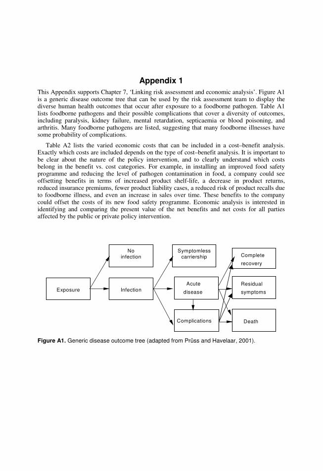
Appendix 1 This Appendix supports Chapter 7, ‘Linking risk assessment and economic analysis’. Figure A1 is a generic disease outcome tree that can be used by the risk assessment team to display the diverse human health outcomes that occur after exposure to a foodborne pathogen. Table A1 lists foodborne pathogens and their possible complications that cover a diversity of outcomes, including paralysis, kidney failure, mental retardation, septicaemia or blood poisoning, and arthritis. Many foodborne pathogens are listed, suggesting that many foodborne illnesses have some probability of complications.
Table A2 lists the varied economic costs that can be included in a cost–benefit analysis. Exactly which costs are included depends on the type of cost–benefit analysis. It is important to be clear about the nature of the policy intervention, and to clearly understand which costs belong in the benefit vs. cost categories. For example, in installing an improved food safety programme and reducing the level of pathogen contamination in food, a company could see offsetting benefits in terms of increased product shelf-life, a decrease in product returns, reduced insurance premiums, fewer product liability cases, a reduced risk of product recalls due to foodborne illness, and even an increase in sales over time. These benefits to the company could offset the costs of its new food safety programme. Economic analysis is interested in identifying and comparing the present value of the net benefits and net costs for all parties affected by the public or private policy intervention.
Figure A1. Generic disease outcome tree (adapted from Prüss and Havelaar, 2001).
Complications
Exposure
Noinfection
Infection
Symptomlesscarriership
Acute
disease
Death
Residual
symptoms
Complete
recovery

116 Appendix 1
Table A1 Chronic complications associated with foodborne pathogens.
Bacterial and parasitic infections transmitted by food
Complications/sequelae
Bacterial infections
Aeromonas hydrophila enteritis Bronchopneumonia, cholecystitis
Brucellosis Aortitis, epididymo-orchitis, meningitis, pericarditis, spondylitis
Campylobacteriosis Arthritis, carditis, cholecystitis, colitis, endocarditis, erythema nodosum, Guillain-Barré syndrome, haemolytic-uraemic syndrome, meningitis, pancreatitis, septicaemia
Escherichia coli (EHEC-types) enteritis
Erythema nodosum, haemolytic-uraemic syndrome, seronegative arthropathy, thrombocytopenic purpura
Q-fever Endocarditis, granulomatous hepatitis
Salmonellosis Aortitis, cholecystitis, colitis, endocarditis, epididymo-orchitis, meningitis, myocarditis, osteomyelitis, pancreatitis, Reiter’s disease, rheumatoid syndromes, septicaemia, splenic abscesses, thyroiditis, septic arthritis (sickle-cell anaemic persons)
Shigellosis Erythema nodosum, haemolytic-uraemic syndrome, peripheral neuropathy, pneumonia, Reiter’s disease, septicaemia, splenic abscesses, synovitis
Vibrio parahaemolyticus enteritis Septicaemia
Yersiniosis Arthritis, cholangitis, erythema nodosum, liver and splenic abscesses, lymphadenitis, pneumonia, pyomyositis, Reiter’s disease, septicaemia, spondylitis, Still’s disease
Parasitic infections
Cryptosporidiosisa Severe diarrhoea, prolonged and sometimes fatal
Giardiasisa Cholangitis, dystrophy, joint symptoms, lymphoidal hyperplasia
Taeniasis Arthritis, cysticercosis (T. solium)
Toxoplasmosis Encephalitis and other central nervous system diseases, pancarditis, polymyositis
Trichinosis Cardiac dysfunction, neurological sequelae
NOTES: (a) Waterborne. SOURCE: Foegeding and Roberts, 1994.
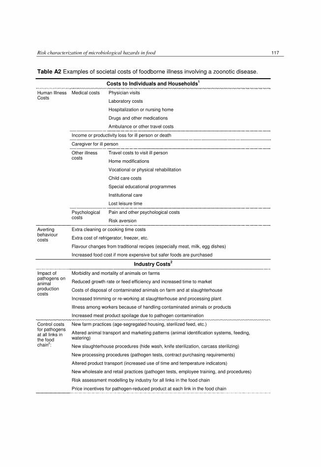
Risk characterization of microbiological hazards in food 117
Table A2 Examples of societal costs of foodborne illness involving a zoonotic disease.
Costs to Individuals and Households1
Medical costs Physician visits
Laboratory costs
Hospitalization or nursing home
Drugs and other medications
Ambulance or other travel costs
Income or productivity loss for ill person or death
Caregiver for ill person
Travel costs to visit ill person Other illness costs
Home modifications
Vocational or physical rehabilitation
Child care costs
Special educational programmes
Institutional care
Lost leisure time
Pain and other psychological costs
Human Illness Costs
Psychological costs
Risk aversion
Extra cleaning or cooking time costs
Extra cost of refrigerator, freezer, etc.
Flavour changes from traditional recipes (especially meat, milk, egg dishes)
Averting behaviour costs
Increased food cost if more expensive but safer foods are purchased
Industry Costs2
Morbidity and mortality of animals on farms
Reduced growth rate or feed efficiency and increased time to market
Costs of disposal of contaminated animals on farm and at slaughterhouse
Increased trimming or re-working at slaughterhouse and processing plant
Illness among workers because of handling contaminated animals or products
Impact of pathogens on animal production costs
Increased meat product spoilage due to pathogen contamination
New farm practices (age-segregated housing, sterilized feed, etc.)
Altered animal transport and marketing patterns (animal identification systems, feeding, watering)
New slaughterhouse procedures (hide wash, knife sterilization, carcass sterilizing)
New processing procedures (pathogen tests, contract purchasing requirements)
Altered product transport (increased use of time and temperature indicators)
New wholesale and retail practices (pathogen tests, employee training, and procedures)
Risk assessment modelling by industry for all links in the food chain
Control costs for pathogens at all links in the food chain2:
Price incentives for pathogen-reduced product at each link in the food chain

118 Appendix 1
Industry Costs2 (contd)
Herd slaughter/product recall
Plant closings and cleanup
Regulatory fines
Product liability suits from consumers and other firms3
Generic animal product - all firms affected Reduced product demand because of outbreak
Reduction for specific firm at wholesale or retail level
Increased advertising or consumer assurances following outbreak
Outbreak costs
Impact of outbreaks on tourism industry
Regulatory and Public Health Sector Costs
Monitor incidence/severity of human disease by foodborne pathogens
Monitor pathogen incidence in the food chain
Disease surveillance costs to
Develop integrated database from farm to table for foodborne pathogens
Identify new foodborne pathogens for acute and chronic human illnesses
Establish high-risk products and production and consumption practices
Identify which consumers are at high-risk for which pathogens
Develop cheaper and faster pathogen tests
Research to
Risk assessment modelling for all links in the food chain
Costs of investigating outbreak
Testing to contain an outbreak (for example, serum testing and administration of IG in persons exposed to Hepatitis A)
Costs of cleanup
Outbreak costs
Legal suits to enforce regulations that may have been violated3
Distributional effects in different regions, industries, etc. Other considerations
Equity considerations, such as special concern for children
NOTES: (1) Willingness-to-pay (WTP) estimates for reducing risks of foodborne disease is a comprehensive estimate of all these categories (assuming that the individual has included employer-funded sick leave and medical programmes in their estimates). The estimate covers reduced risks for all exposed persons: those who will become ill as well as those who will not. (2) Some industry costs may fall with better pathogen control, such as reduced product spoilage, possible increases in product shelf-life, and extended shelf-life permitting shipment to more distant markets or lowering shipment costs to nearby markets. (3) In adding up costs, care must be taken to ensure that product liability costs to firms are not already counted in the estimated pain and suffering cost to individuals. However, the legal and court expenses incurred by all parties are social costs. SOURCE: Adapted from Buzby and Roberts, 1997.
Risk characterization of microbiological hazards in food 119
References
Buzby, J.C. & Roberts, T. 1997. Economic costs and trade impacts of food borne illness. World Health Statistics Quarterly, 50: 57–66.
Foegeding, P.M. & Roberts, T. 1994. Food borne Pathogens: Risks and Consequences. Prepared by the Co-chairs, Council for Agricultural Science and Technology Task Force. Ames, USA: Council for Agricultural Science and Technology. 87 p.
Prüss, A. & Havelaar, A.H. 2001. The global burden of disease: study and applications in water, sanitation and hygiene. pp. 43–60, in: L. Fewtrell and J. Bartram (editors). Water Quality: Guidelines, Standards & Health: Risk assessment and management for water-related infectious disease. London, UK: IWA Publishing.

FAO/WHO MICROBIOLOGICAL RISK ASSESSMENT SERIES
1 Risk assessments of Salmonella in eggs and broiler chickens: Interpretative Summary, 2002
2 Risk assessments of Salmonella in eggs and broiler chickens, 2002
3 Hazard characterization for pathogens in food and water: Guidelines, 2003
4 Risk assessment of Listeria monocytogenes in ready-to-eat foods: Interpretative Summary,
2004
5 Risk assessment of Listeria monocytogenes in ready-to-eat foods: Technical Report, 2004
6 Enterobacter sakazakii and microorganisms in powdered infant formula: Meeting Report,
2004
7 Exposure assessment of microbiological hazards in food: Guidelines, 2008
8 Risk assessment of Vibrio vulnificus in raw oysters: Interpretative Summary and Technical
Report, 2005
9 Risk assessment of choleragenic Vibrio cholerae 01 and 0139 in warm-water shrimp in
international trade: Interpretative Summary and Technical Report, 2005
10 Enterobacter sakazakii and Salmonella in powdered infant formula: Meeting Report, 2006
11 Risk assessment of Campylobacter spp. in broiler chickens: Interpretative Summary, 2008
12 Risk assessment of Campylobacter spp. in broiler chickens: Technical Report, 2008
13 Viruses in food: Scientific Advice to Support Risk Management Activities: Meeting Report, 2008
14 Microbiological hazards in fresh leafy vegetables and herbs: Meeting Report, 2008
15 Enterobacter sakazakii (Cronobacter spp.) in powdered follow-up formula: Meeting Report, 2008
16 Risk assessment of Vibrio parahaemolyticus in seafood: Interpretative Summary and Technical
Report, 2010
17 Risk characterization of microbiological hazards in food: Guidelines, 2009.

Publications of the World Health Organizationcan be obtained from:
WHO PressWorld Health Organization, 20 Avenue Appia
CH-1211 Geneva 27, SwitzerlandTel: +41 22 7913264Fax: +41 22 7914857
E-mail: [email protected]
on the Internet from http://www.who.int/bookorders
Publications of the Food and Agriculture Organization of the United Nations can be ordered from:
Sales and Marketing Group, Communication DivisionFood and Agriculture Organization of the United Nations
Viale delle Terme di Caracalla, 00153 Rome, Italy Fax: +39 06 57053360
E-mail: [email protected] or
on the Internet from http://www.fao.org/icatalog/inter-e.htm
Printed in Italy
Risk characterization is one of the four steps of microbiological risk assessment. It is defined as an estimation of the probability of occurrence and severity of known or potential adverse health effects in a population based on the preceding steps of hazard identification, hazard characterization and exposure assessment. It comprises the results of the risk assessment in the form of risk estimates and risk descriptions and provides the best available science-based evidence to support food safety management.
This volume presents guidelines for risk characterization of microbiological hazards in foods. These guidelines provide descriptive guidance on how to conduct risk characterization in various contexts, and utilizing a variety of tools and techniques. They have been developed in recognit ion of the fact that a reliable estimation of risk is critical to the overall risk assessment.
Th i s vo lume and o the rs i n t h i s M i c rob io l og i ca l R i sk Assessment Series contain information that is useful to both risk assessors and risk managers, including international scientific committees, the Codex Alimentarius Commission, governments and food regulatory agencies, scientists, food producers and industries and other people or institutions with an interest in the area of microbiological hazards in foods, their impact on human health and food trade and their control.
9 7 8 9 2 5 1 0 6 4 1 2 2I1134E/1/11.09/1500
ISBN 978-92-5-106412-2 ISSN 1726-5274