MICROECONOMICS I: CHOICE UNDER UNCERTAINTY

MARCIN PĘSKI

Please let me know about any typos, mistakes, unclear or ambiguous statementsthat you find.

1. Introduction

1.1. Suggested readings. MWG chapter 6.A. Kreps “Notes on the Theory of Choice”,chapters 4 and 7 (the first part only).

1.2. Describing the uncertainty.

Example 1. A company develops a product of an unknown quality. The productcan be either good or bad. Company manager must decide whether to advertise theproduct or not. The payoffs (say, in monetary units) for the manager are

˙good badAdvertise 10 −1

Don’t advertise 0 0

The manager’s choice will reveal his preferences over the two actions.In this example, the agent chooses between a pair of decisions “Advertise” and

“Don’t advertise”. Each decision is described by a pair of numbers cb and cg thatdenote the monetary consequences of the decision given one of two states of theworld, b and g.

We are going to assume that the pair of numbers (cb, cg) contains all the informationnecessary for the manager to make the decision. The assumption can be divided intotwo logically independent (sub) assumptions:

• there are only two states of the world that are relevant for the problem athand,• the monetary payoffs in each state describe all the relevant consequences ofthe decision.

1

2 MARCIN PĘSKI

payoffs in state b

payoffs in state g

(cb, cg)

cb

cg

Figure 1.1. Space of acts, S = {cb, cg} , Z = R.

Mathematically, the pair of numbers can be represented as a mapping from the spaceof the states of the world S = {b, g} into the space of “prizes” (i.e., monetary conse-quences) Z = R. Each mapping of this form c : S → R can be described as a pair ofnumbers c = (cb, cg). We refer to such objects as acts and let A = ZS be the space ofthe acts.

With only two states, we can represent the space of acts on a two-dimensionaldiagram.

1.3. Preferences. The decision theory under uncertainty is a continuation of thedecision theory that you learned in the beginning of the course. In particular, as inthe standard decision theory, we typically make two assumptions:

• The decision maker has well-defined preferences � over acts. That implies(and is almost implied by) that the choices over the acts satisfy WARP.

We can use our diagram of the space of the acts to describe preferences o the manager,or at least draw her indifference curves. For example, if the manager prefers moremoney, then the indifference curves will be downward sloping (see Fig. Indifferencecurves).

• The preferences are continuous. Then, the utility theory (Proposition 3.C.1from MWG) says that there exists a utility representation of the preferences�:

UNCERTAINTY 3

state b

state g

(cb, cg)

cb

cg

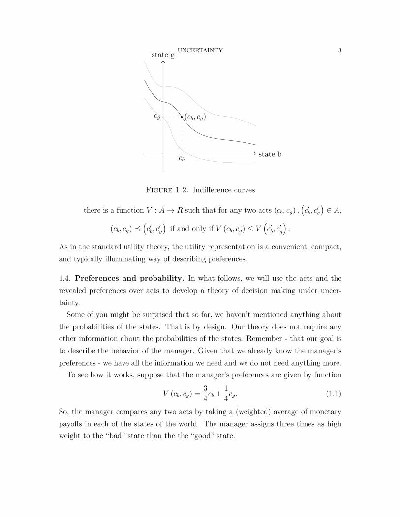
Figure 1.2. Indifference curves

there is a function V : A→ R such that for any two acts (cb, cg) ,(c′b, c

′g

)∈ A,

(cb, cg) �(c′b, c

′g

)if and only if V (cb, cg) ≤ V

(c′b, c

′g

).

As in the standard utility theory, the utility representation is a convenient, compact,and typically illuminating way of describing preferences.

1.4. Preferences and probability. In what follows, we will use the acts and therevealed preferences over acts to develop a theory of decision making under uncer-tainty.

Some of you might be surprised that so far, we haven’t mentioned anything aboutthe probabilities of the states. That is by design. Our theory does not require anyother information about the probabilities of the states. Remember - that our goal isto describe the behavior of the manager. Given that we already know the manager’spreferences - we have all the information we need and we do not need anything more.

To see how it works, suppose that the manager’s preferences are given by function

V (cb, cg) = 34cb + 1

4cg. (1.1)

So, the manager compares any two acts by taking a (weighted) average of monetarypayoffs in each of the states of the world. The manager assigns three times as highweight to the “bad” state than the the “good” state.

4 MARCIN PĘSKI

There are many different reasons why the manager could have had such a prefer-ences. Consider the following two examples:

• The manager cares only about the expected payoff from her decision. Themanager is very experienced and she knows that 75% of the time the stateof the world is bad. She applies her experience to the problem at hand toestimate that the probability that the state is “bad” is equal to 3

4 .• The manager cares only about the expected payoff from her decision. Sheis a new manager on her first managerial position. She doe snot have anyexperience to estimate the probability of the “bad” state. She does not wantto mess up, and she believes that she can reduce the chances of it is safer toassign higher weights to “bad” states of the world. The exact value of theweight, 3

4 , is taken from looking at the ceiling.• The manager is a computer program designed by an engineer in a differentcountry who was told by his boss to come up with some reasonable formulafast, no matter what as long as it is reasonable. The engineer picked up someformula from Wikipedia.• If the state is “good”, her utility is equal to cg. If the state is “bad”, herutility is equal to 1

2cb (because, possibly, her company will =go bankrupt withprobability 1

2 , in which case, she gets no profits at all). She assigns probability67 to the “bad” state. Her utility from profits in a bad state is equal to 1

2cb.The manager cares about the expected utility:

67

(12cb

)+ 1

7cg = 37cb + 1

7cg = 47

(34cb + 1

4cg)

= 47V (cb, cg) .

Notice that the above formula describes the same preferences as (1.1) - if wemultiply utility function by a positive constant, the preferences are unchanged.

Each of the above cases describes different reasons why the manager has preferencesrepresented by (1.1). Only in the first case, we can say that parameter 3

4 can be inter-preted as a probability of the state. Nevertheless, each of the cases above (includingthe first one) leads to the same preferences, and hence, the same decision theory.

We emphasize that the “probabilities” are not necessary for any decision theory. Ifwe can interpret the preferences as if they arose from some probabilistic model of the

UNCERTAINTY 5

state b

state g

(cb, cg)

cb

cg

Figure 1.3. Indifference curves for expected payoff representation

world, that’s great for us and it is helpful. But, the probabilities are nothing more(and nothing less) than that - interpretation.

More generally, all decision theory proceeds as follows: Find conditions (i.e., knownas “axioms”) on the behavior (i.e., preferences) that guarantee that the behavior canbe interpreted as if the decision maker acts according to some model (for example,expected utility). The model is an interpretation, “as if”, and it does not reallyhave to correspond to anything that “really” happens in the world (say, whether thedecision maker in her brain computes the probabilities).

We need to remember this remark when we study the expected utility models.

1.5. Examples of utility representations. We list and compare few types of util-ity representations.

Expected payoff. Suppose that

V (cb, cg) = pcb + (1− p) cg

for some p ∈ [0, 1]. The indifference curves are linear (Fig. 1.3), and the slope dependson p.

We can interpret p as a “probability” (we will talk about what exactly it meanslater) of the state “good”. Then, V is the expected payoff from an act.

6 MARCIN PĘSKI

state b

state g

(cb, cg)

cb

cg

Figure 1.4. Indifference curves for the Maxmin representation

Expected utility. Let u : R → R be a standard (increasing, continuous) utility frommonetary payoffs. Suppose that

V (cb, cg) = pu (cb) + (1− p)u (cg) . (1.2)

We say that V is the expected utility representation with (state-independent) utilityfunction u and probabilities p for the “good” state.

Be careful to distinguish utility over acts V (.) and “small” utility u (.) from con-sumption given a state!

Exercise 1. Is it possible that the indifference curves of model (1.2) look like thosedrawn on Fig. 1.2? Draw the indifference curves if you know that u () is concave.

Maxmin utility. Suppose that

V (cb, cg) = min {cb, cg} .

Here, V (cb, cg) is equal to the payoff in the worst possible state. The manager choosesto maximize the worst possible payoff. There is no probabilities in the representation- they are not relevant. The only relevant thing is the worst possible payoff. Theindifference curves look like the indifference curves in the Leontieff utility - they havea corner on 45 degree line (see Fig. 1.4).

UNCERTAINTY 7

State-dependent utility.

Example 2. Alan likes ice cream and he wants to eat some ice cream tomorrow. Bethis able to provide the ice cream for Alan, but her offer is contingent on tomorrow’sweather. There are two possible states “sun” and “rain”. Beth offers two “insuranceplans”:

˙sun rainplan 1 2 0plan 2 1 1

Alan must choose today, before tomorrow’s weather is known (and he is committedto his choice).

Alan’s choice, intuitively will depend on

(1) how likely is each of the states of the world,(2) how much he likes more ice cream vs. less (i.e., his marginal utility of ice

cream), and(3) how much he likes ice cream given the weather.

One example of Alan’s preferences is state-dependent expected utility:

V (c1, c2) = pub (cb) + (1− p)ug (cg) (1.3)

Notice that the utility function depends on the state.The representation (1.3) is somehow misleading in that it suggests a well-defined

probability distribution over states. However, notice that if p ∈ (0, 1) we write downan equivalent representation for any other p′ ∈ (0, 1). Indeed, define functions

u′b (cb) = p

p′ub (cb) ,

u′g (cg) = 1− p1− p′ug (cq) .

Then,

V (cb, cg) = p′p

p′ub (cb) + (1− p′) 1− p

1− p′ug (cg)

= p′u′b (cb) + (1− p′)u′g (cg) .

8 MARCIN PĘSKI

In other words, we can represent preferences V with two different sets of probabilitiesand state-dependent utility functions. Because both representations lead to exactlythe same choices, there is no way that we can tell which representation is more correct.

For this reason, it is more appropriate to incorporate the probabilities in the defi-nition of utility functions. Let

u′′b (cb) = pu (cb) and u′′g (cg) = (1− p)u (cg) .

Then,

V (cb, cg) = u′′b (cb) + u′′g (cg) . (1.4)

We refer to the additive form (1.4) as the state-dependent utility.To summarize, the state-dependent utility representation does not determine the

probabilities over states.

2. Model

2.1. Subjective vs. objective uncertainty. The nice thing about our approachso far is that we do not need to make any assumptions about the true probabilitiesof the states. The only thing that matters are the preferences of the agent. In fact,we can try to identify the probabilities from the agent’s preferences (see Section 1.4).

There is a fundamental difference about the concept of probability that we discusshere, and that is inferred from revealed choices of an individual, and the more familiarconcept of the probability of the fact that the coin will fall Heads. The former is called“subjective” to emphasize the fact that it exists only in the mind of the individual(and only if we are willing to treat our interpretation as something more than “asif”). The other is “objective” - it can be measured, tested, repeated, etc.

From now on, we will distinguish between two types of probabilities: “subjective”and “objective”. Our model of objective probabilities has four elements:

(1) The space of states S. The state space contains all possible realizations of theworld. Or, more precisely, all possible and relevant to the choice at hand (theassumption that the agent is able to conceive all possible states of the worldis often criticized, because there is too many of them.)

UNCERTAINTY 9

(2) The set of “prizes” Z. The prizes are things that directly affect our utility(consumption in monetary terms, amount of ice-cream, etc.)

(3) Acts: an act is a function f : S → Z. The interpretation is that f (s) is a“prize” that the agent receives if the true state of the world turns out to be s.This definition of an act was introduced by L. Savage, so we call them Savageacts, to distinguish from other type of acts (we will see the other ones soon).An example of an act, is a constant act δz that specifies the same prize z ineach of the state of the world, δz (s) = z for each s ∈ S.

(4) Preference relation � over acts. Specifically, for any two acts fand g, f � g

means that the agent (weakly) prefers act f to g.For simplicity, we assume that S and Z are finite.

We won’t make any assumption about the probabilities over states S, in fact wewill try to infer it from the preferences.

However, we will assume that the individual agrees on the objective probabilitiesof some events. For example, we assume that the individual understands that the faircoin falls Heads with probability 1

2 and that the dice shows 6 with probability 16 .

We are going to distinguish the objective probabilities by defining lotteries. Alottery is a probability distribution over prizes q ∈ ∆Z. Hence, q (z) is a objectiveprobability of receiving prize z.

Example 3. Suppose that you have a raffle ticket that wins with probability 1100 .

The prize in the raffle is a free dinner in the best restaurant in town. We repre-sent the ticket using a two-element set Z = {dinner, nothing} and a lottery q ="dinner" 1

100 "nothing" 99100 such that q (dinner) = 1

100 and q (nothing) = 99100 .The key here

is that there is an objective probability with which the ticket wins. The objectivityhere means that both the agent and the modeler and everybody else agree on theexact value and the nature of the probabilities.

2.2. Anscombe-Aumann acts. We are going to combine the subjective and objec-tive probability in one model by extending our definition of an act: Instead of prizes,we assume that the act specifies lotteries over prizes given each state. Formally, anAnscombe-Aumann act (AA act, for short) is a mapping f : S → ∆Z with the inter-pretation that f (s) is an (objective) lottery which the agent receives if the state of

10 MARCIN PĘSKI

the world turns out to be s, and f (s) (z) is an objective probability with which theagent receives prize z if the world is s.

The distinction between subjective and objective uncertainty that lies at the heartof AA act should be clear at the theoretical, or conceptual levels. It is not so clearin the “real life”, where it is often difficult to draw a border between two types ofuncertain. One can construct some examples (For instance: Let

S = {cure for cancer within next 20 years, no cure for cancer within next 20 years} .

For each state s, the life length is a lottery with a distribution that can be easilycomputed from the mortality tables and an information about the reasons for eachdeath. The probability of state s ∈ S is not so easy to determine), but these examplesare more often than not somehow artificial or forced.

On the other hand, our theory simply is going to assume that the decision makeris able to rank the AA acts Kreps says that the lotteries and AA acts are more oftenthan not thought exercises than real objects. That’s OK with us.

Do we need AA acts to develop a decision theory? No. Savage developed hiswhole expected utility theory without worrying about objective probabilities. But,his theory is difficult. AA acts make our life much easier. Why? Roughly, becausethey provide more data for our theory. To see it, notice first that there are more AAacts than Savage acts. (Each Savage act is an AA act with a degenerate lotteries ineach state.) So, if we observe the preferences over all AA acts, we get much moreinformation about the rankings than if we could only observe the preferences overSavage acts.

2.3. Compound acts and convex combination of acts. One of the reason whyworking with AA acts is easier is that the space of AA acts can be equipped with anatural operation of taking convex combinations. It turns out that (a) this operationis very useful mathematically and (b) it has a somehow natural interpretation. Forany α ∈ [0, 1], for any two acts f and g, define an act αf ⊕ (1− α) g so that for eachs and z,

(αf ⊕ (1− α) g) (s) (z) := αf (s) (z) + (1− α) g (s) (z) . (2.1)

UNCERTAINTY 11

This left-hand side is the (objective) probability that the agent receives prize z instate s given the act αf ⊕ (1− α) g. The right hand side is a convex combinationwith weight α of the probability of prize z given state s and acts f and g. In otherwords, is a well-defined act.

We still need to check whether αf ⊕ (1− α) g , the convex combination of two actsf and g with the weight α on the first act, is a well-defined act. That means, we needto check whether it assigns well-defined lotteries to each state. But,∑

z

(αf ⊕ (1− α) g) (s) (z)

=∑z

αf (s) (z) +∑z

(1− α) g (s) (z)

=α + (1− α) = 1.

So, we are good.Mathematically, the above operation corresponds to taking convex combinations.

There is also another, natural even if somewhat subtle interpretation. We will describethe interpretation very carefully to make sure that we understand what it says andwhat it does not say. First, notice that for any two acts f and g, and for anynumber α ∈ [0, 1], we can consider a lottery over two acts fαg1−α. The lottery isobjective (hence, the probability is known and well-understood) and with probabilityα chooses act f and with probability 1− α chooses act g. We refer to such a lotteryas a “compound act” and we can interpret it as just another (a slightly more generalversion of) act.

Second, the right-hand side of (2.1) is a probability of prize z in a equivalent reducedlottery with the timing of uncertainty reversed: first, Nature decides on the state s,then we draw with probabilities α and 1− α the lotteries, respectively, f (s) or g (s),and then, finally, we use the drawn lottery to draw the prize. Thus, we can thinkabout (αf ⊕ (1− α) g) (s) as a reduced form of the compound act fαg1−α.

To see how it works, consider the following example.

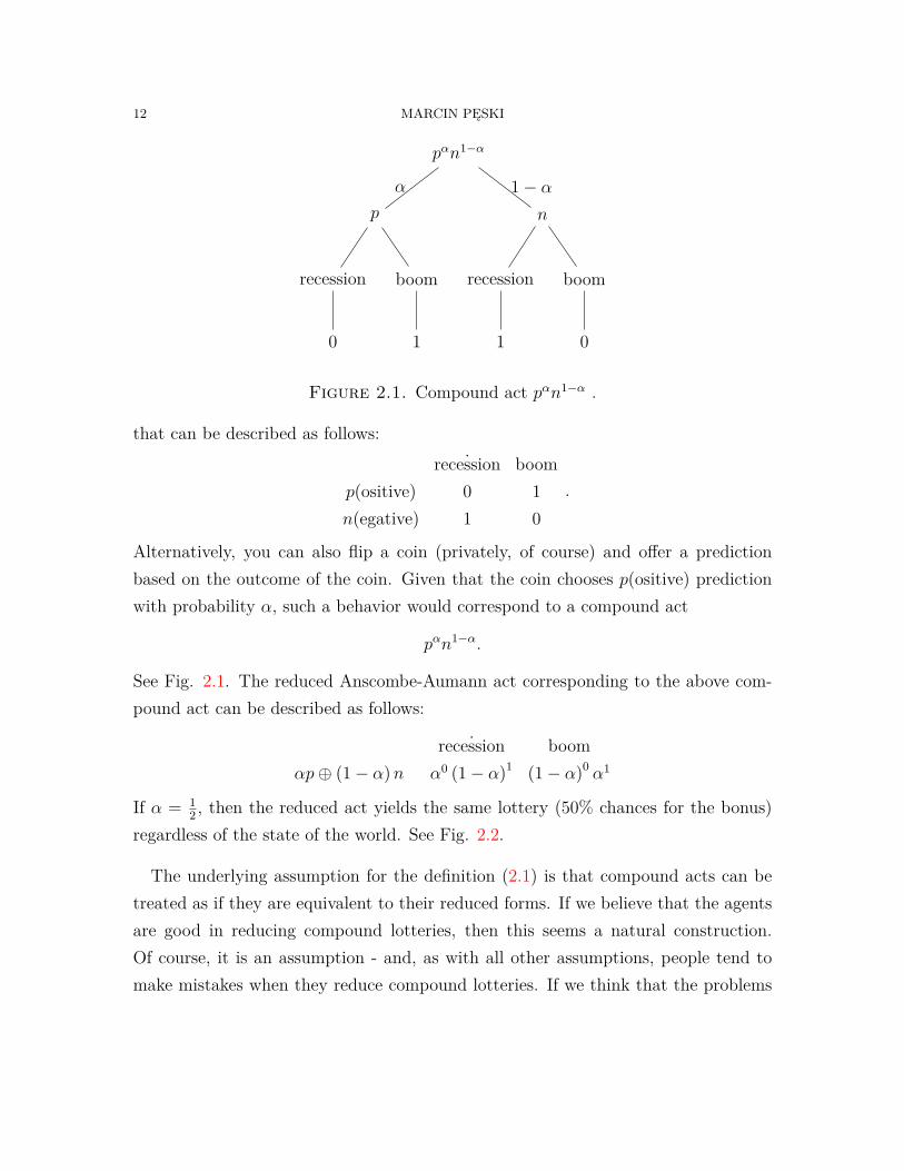
Example 4. You are an analyst in a macro consulting firm. You are asked to makea prediction about the future state of economy. if your prediction turns out to becorrect, but only if so you will get a bonus. In short, you choose between two acts

12 MARCIN PĘSKI

pαn1−α

p

recession

0

boom

1

α

n

recession

1

boom

0

1− α

Figure 2.1. Compound act pαn1−α .

that can be described as follows:˙recession boom

p(ositive) 0 1n(egative) 1 0

.

Alternatively, you can also flip a coin (privately, of course) and offer a predictionbased on the outcome of the coin. Given that the coin chooses p(ositive) predictionwith probability α, such a behavior would correspond to a compound act

pαn1−α.

See Fig. 2.1. The reduced Anscombe-Aumann act corresponding to the above com-pound act can be described as follows:

˙recession boomαp⊕ (1− α)n α0 (1− α)1 (1− α)0 α1

If α = 12 , then the reduced act yields the same lottery (50% chances for the bonus)

regardless of the state of the world. See Fig. 2.2.

The underlying assumption for the definition (2.1) is that compound acts can betreated as if they are equivalent to their reduced forms. If we believe that the agentsare good in reducing compound lotteries, then this seems a natural construction.Of course, it is an assumption - and, as with all other assumptions, people tend tomake mistakes when they reduce compound lotteries. If we think that the problems

UNCERTAINTY 13

αp⊕ (1− α)n

recession

p (recession)

0

α

n (recession)

1

1− αboom

p (boom)

1

α

n (boom)

0

1− α

αp⊕ (1− α)n

recession

0α11−α

boom

01−α1α

Figure 2.2. Reduced act αp⊕ (1− α)n (right side).

with reducing compound lotteries are important, then the construction (2.1), or moreprecisely, the axioms based on this construction, will tend to be violated. We will goback to this issue soon.

So far, we used symbol ⊕ to describe the convex combination. We did this toemphasize the conceptual difference between compound acts and reduced acts. In thesame time, as the above discussion suggests, from now on we will typically interpretboth operations as the same. For this reason, it will be easier to use one symbol.From now on, we will write simply αf + (1− α) g instead of αf ⊕ (1− α) g.

2.4. Two states, two prizes representation. Suppose that the sets of prizes andstates contain two elements each. Specifically, suppose that Z = {a, b}, and S ={s1, s2}.

An Anscombe-Aumann act assigns probability distribution over the prizes to eachof the states. So, f (a|s) is the probability of receiving prize a in state s. Becausef (b|s) = 1− f (a|s), we can deduce the probability of prize b from the probability ofa. In other words, the knowledge of probabilities f (a|s) for each state s is enough tocharacterize an act.

Because f (a|s) ∈ [0, 1] for each state, we can interpret the Anscombe-Aumann actf ∈ F as a point in the “consumption space” X = [0, 1]2 with the interpretation that

14 MARCIN PĘSKI

(f1, f2) ∈ X corresponds to the act f such that

f (a, s1) = f1, f (b|s1) = 1− f1,

f (a, s2) = f2, f (b|s2) = 1− f2,

For example, act f =(

12 , 0

)∈ X means that the individual receives prize a with

probability 12 if the state is 1, and receives prize b with probability 1 if the state is 2.

Notice that for any two acts f, g ∈ F , the convex combination of two acts, αf +(1− α) g, corresponds to the convex combination of the points in space X,

α (f1, f2) + (1− α) (g1, g2) = (αf1 + (1− α) g1, αf2 + (1− α) g2) .

Now, the preferences over AA acts can be represented using the familiar diagramswith indifference curves.

2.5. Purely objective theory (MWG). The first development of the expectedutility was purely objective. In fact, the discussion of the expected utility theory thatyou can read in MWG follows the purely objective path.

You will be happy to learn that our present model is strictly more general. Tosee why, notice that you can eliminate subjective uncertainty by assuming that thestate space S contains a single element, say S = {∗}. In such a case, an AA actf : S → ∆Z is equivalent to an objective lottery f (∗) = q ∈ ∆Z. The decisionmaker’s preferences over acts are equivalent to preferences over (objective) lotteries.

You may worry that given that our theory is more general, it is also going to bemore complicated. Worry not! It turns out that we have already learned the maindifference between theories - the idea of AA act. Everything else, including the axiomsand the proofs that you will see in the next section, follow almost exactly the samelines.

Graphical representation with three prizes Z = {a, b, c}!

3. State-Dependent Expected Utility

3.1. Suggested readings. MWG chapter 6.B., Kreps “Notes on the Theory ofChoice”, chapter 7.

UNCERTAINTY 15

3.2. Model. Model:

(1) Finite state space S.(2) Finite set of prizes Z. The set of lotteries over prizes ∆Z (i.e., the set of

probability distributions over Z.(3) (Anscombe-Aumann acts): functions f : S → ∆Z. Let F be the space of

acts.(4) Binary relation � over acts. The theory assumes that we can observe the

agent choices over pairs of AA acts. The choices reveal the relation �.

3.3. Representation. We say that relation � has a state dependent expected utility(SDEU) representation if and only if there exist functions us : Z → R such that forany two acts f and g,

f � g iff∑s,z

us (z) fs (z) ≤∑s,z

us (z) gs (z) .

We say that relation� has a state independent expected utility (SIEU) representationif and only if there exist function u : Z → R and probability distribution π ∈ ∆Ssuch that for any two acts f and g,

f � g iff∑s,z

πsu (z) fs (z) ≤∑s,z

πsu (z) gs (z) .

3.4. Axioms. Axiom 1. (Preference) Binary relation � is a rational preferencerelation (i.e., it is transitive and complete).

The first axiom is obvious. Because � is a preference relation, we can use it todefine the relations of strict preference ≺ and indifference ∼.Axiom 2. (Continuity) For each act g ∈ F , the upper and the lower contour

sets of g,

{f : g � f} and {f : f � g}

are closed.

16 MARCIN PĘSKI

1

The Continuity Axiom is a version of the same axiom that we used in the utilitytheory to prove the existence of continuous utility representation.Axiom 3. (Independence). For any three acts f, g, h, if f ≺ g, then for any

α ∈ (0, 1), αf + (1− α)h ≺ αg + (1− α)h.The axiom seems natural: taking convex combination with the same act should

not change the preference relations. This is the key axiom of the theory.To understand the axiom a little bit better, take three acts three acts f, g, h, and

suppose that the decision maker prefers act f to act g, f ≺ g. Next, considercompound acts fαh1−α and gαh1−α. The two compound acts are obtained by alottery with probability α acts, respectively, f or g, and with probability 1−α act h.We make two claims:

(1) If the decision maker’s preferences were defined over the compound acts (andnot only over the AA acts), our decision maker would rank the compound actsin the same way as the original acts, i.e. she would prefer fαh1−α to gαh1−α.

(2) The ranking over the compound acts should be the same as the ranking overtheir reduced versions, αf + (1− α)h and αg + (1− α)h.

Claim 1 can be explained by the fact that the two compound acts differ only inthe event drawn with probability α, in which case the difference is equivalent to thedifference between acts f and g. Claim 2 follows from our discussion from section 2.3about the equivalence of compound acts and their reduced versions. If you believethat the two claims are correct, you must accept the Independence Axiom.

Example 5. Recall the situation from Example 4. Suppose that the manager hasno clue which of the recession or boom is more likely. In fact, he may treat the twoevents completely symmetrically. In such a case, he would be indifferent between twoacts p and n. Also, as in Claim 1, the manager is indifferent between choosing p,n, or flipping a coin and choosing the prediction based on the outcome of the coin.Using our terminology, he is indifferent p 1

2n12 .

1The literature usually describes a slightly weaker axiom, called Archimedean: For any three actsf ≺ g ≺ h, there exist sufficiently small a, b ∈ (0, 1) such that af + (1− a) h ≺ g ≺ bh + (1− b) f .We use the stronger version to compare to the consumer utility theory and for simplicity.

UNCERTAINTY 17

Further, suppose that the manager is not only utterly unqualified, but also veryconfident and he expects that given otherwise equal odds, the Nature is going to beon his side (that is not supposed to be a precise statement, but rather a description ofa psychological state of his mind. I am sure that you know people like this). It seemsat least plausible that such a manager would prefer act p 1

2n12 to its reduced version

12p + 1

2n. In the former case, he believes that the sympathetic Nature will help himto win; in the latter case, the Nature has no chances in manipulating the objectivelottery. Such a manager will fail Claim 2 and the Independence Axiom.

In this example, the manager fails Claim 2 because he prefers the uncertainty abouthis decision to be resolved before Nature chooses the state of the world. Later, insection 5.2, we will see a slightly different (in some sense, opposite) type of violationof the Independence Axiom.

Of course, if you don’t believe Claim 1 or Claim 2 (for example, because you don’tthink that people are able quickly reduce compound lotteries, or because their attitudeto the timing of the resolution of uncertainty), you won’t believe the IndependenceAxiom. As we will prove soon, it turns out that if you don’t believe the IndependenceAxiom, you must think that the decision maker is not an expected utility maximizer.

3.5. Main result.

Theorem 1. Relation � has a state dependent utility representation if and only if itsatisfies Axioms 1,2,3.

Thus, by testing Axioms 1,2, and 3, we can test (more precisely, reject) the state-dependent theory.2 The second part of the Theorem is also called invariance to affinetransformations.

2The axioms are stated in such a way that they can be tested, in a particular way. An axiomcan be violated by pointing to a pair (or triple) of acts for which the agent chooses differently fromwhat the axiom says. The violation of the axioms means that the expected utility theory must berejected.

We cannot imagine a real world experiment that would allow us to accept the expected utilitytheory. The problem, of course, is that the set of acts is infinite and we cannot possibly ask theagent to list all possible choices over all pairs of acts.

18 MARCIN PĘSKI

3.6. Proof.

Exercise 2. Show that if relation � has a state dependent utility representation,then it satisfies Axioms 1,2, and 3.

We will show that Axioms 1, 2, and 3 imply the state-dependent utility repre-sentation. The proof has two basic steps. The first step is to find an affine utilityrepresentation of relation �. We show that there exists a function F : F → R suchthat (a) F represents �: for any two acts f and g,

f � g iff F (f) ≤ F (g) ,

and (b) F is affine: for any two acts f and g, and for any number α ∈ (0, 1),

F (αf + (1− α) g) = αF (f) + (1− α)F (g) . (3.1)

In the second step, we show that there exist functions us : Z → R such that for anyact f ,

F (f) =∑s,z

us (z) fs (z) . (3.2)

Parts (a) and (b) together establish the existence of state-dependent representation.

3.6.1. Affine utility representation. We start with some preliminary results.

Lemma 1. There exists acts f ∗ and g∗ such that for any act h, f ∗ � h � g∗.

The acts f ∗ and g∗ are respectively the worst and the best act.

Proof. Due to Axiom 1 and 2, the (standard) utility theory shows that there existsa continuous utility function U : F → R that represents preferences on acts f ∈ F .Because the space of acts is compact, there exists

f ∗ ∈ arg minf∈F

U (f) and g∗ ∈ arg maxf∈F

U (f) .

Because function U represents the preferences, the two acts are respectively, the worstand the best act. �

Lemma 2. For any two acts f ≺ g, any α, β ∈ (0, 1) ,α > β if and only if αf +(1− α) g ≺ βf + (1− β) g.

UNCERTAINTY 19

Proof. Suppose that α > β. Notice first that Axiom 2 implies that

αf + (1− α) g ≺ αg + (1− α) g = g.

Using Axiom 3 again, we get

βf + (1− β) g = β

α(αf + (1− α) g) +

(1− β

α

)g

� β

α(αf + (1− α) g) +

(1− β

α

)(αf + (1− α) g)

= αf + (1− α) g.

The other direction follows from a similar argument applied to α ≤ β. �

Lemma 3. Suppose that f ∗ ≺ g∗. For each act h, there exists unique αh ∈ [0, 1] suchthat h ∼ αhg

∗ + (1− αh) f ∗.

The Lemma says that any act that lies between f and g (in the sense of preferencerelation) can be calibrated to some mixture of acts f and g.

Proof. The result holds trivially if h ∼ g∗ or h ∼ f ∗. So, assume that f ∗ ≺ h ≺ g∗.Recall that the preferences have a continuous utility representation U . Let u : [0, 1]→R be defined as

u (α) = U (αg∗ + (1− α) f ∗) .

Then, u is continuous and u (0) = U (f ∗) < U (h) < U (g∗) = u (1). By the interme-diate value theorem, there exists αh ∈ (0, 1) such that

U (h) = u (αh) = U (αhg∗ + (1− αh) f ∗) .

�

We use the Lemmas to prove our claim. Let f ∗ and g∗ be as in Lemma 1. Theclaim holds trivially when f ∗ ∼ g∗ (or, in other words, the decision maker is indifferentamong all acts). So, now we assume that f ∗ ≺ g∗.

• Define function F using Lemma 3: For each act h, let F (h) = αh.

20 MARCIN PĘSKI

• Property (a) follows from the equivalence of the sequence of claims for anytwo acts h and h′:

h � h′,

⇐⇒by definition of α αhg∗ + (1− αh) f ∗ � αh′g

∗ + (1− αh′) f ∗

⇐⇒by Lemma 3 αh ≤ αh′

⇐⇒by definition of F (.) F (h) ≤ F (h′) .

• Property (b) follows from the following observations. Take f ∗ � h � h′ � g∗.Then, for any x ∈ [0, 1], by Lemma 3 and the definition of function F (fill allthe remaining steps),

xh+ (1− x)h′

∼ x((1− F (h)) f ∗ + F (h) g∗) + (1− x) ((1− F (h′)) f ∗ + F (h′) g∗)

= [x (1− F (h)) + (1− x) (1− F (h′))] f ∗ + [xF (h) + (1− x)F (h′)] g∗.

But this implies that

F (xh+ (1− x)h′) = xF (h) + (1− x)F (h′) .

3.6.2. State-dependent expected utility. We start with few definitions. First, we fixone price z∗ ∈ Z and let

z∗=δz∗= (z∗, ..., z∗)

be a constant act that always yields prize z∗. Next, for each price z ∈ Z and eachstate s ∈ S, define deterministic act

fz,s = (z∗, ..., z∗, zstate s , z∗, ..., z∗) .

In other words, act fz,s yields prize z in state s and prize z∗ in any other state s′ 6= s.Let F (fz,s) be the value of act fz,s according to function F . And, finally, define

us (z) = F (fz,s)−n− 1n

F (z∗) .

We will show that (3.2) is satisfied. We will do it in two short steps. First, wewill show the claim for deterministic act f , i.e., f (s) = zs ∈ Z for each state s. Letn = |S| be the number of states. To shorten the notation, we assume that we can

UNCERTAINTY 21

enumerate all states s ∈ S from 1 to n. Notice that the mixture act 1nf + n−1

nz∗ is

equal to the mixture (with equal weights) of acts fz1,1, ..., fzn,n.1nf + n− 1

nz∗ =

( 1nz1 + n− 1

nz∗, ...,

1nzn + n− 1

nz∗)

= 1n

(z1, z∗, ..., z∗)

+ 1n

(z∗, z2, ..., z∗)

+ ...

+ 1n

(z∗, ..., z∗, zn)

= 1nfz1,1 + 1

nfz2,2 + ...+ 1

nfzn,n

By repeated application of (3.1),1nF (f) + n− 1

nF (z∗) =F

( 1nf + n− 1

nz∗)

= 1nF (fz1,1) + ...+ 1

nF (fzn,n)

= 1n

(u1 (z1) + ...+ un (zn)) + n− 1n

F (z∗) .

But this implies thatF (f) = u1 (z1) + ...+ un (zn) .

To conclude, we need to show (3.2) holds for all acts, not necessarily deterministic.We leave this part as an exercise.

3.7. Invariance to affine transformations.

Theorem 2. Collections of functions (us) and (vs) are two SDEU representations ofthe same preference relation if and only if there exists constant a > 0 and bs ∈ R foreach state s such that for each s, vs = aus + bs.

Proof. In the exercise, you are asked to show that a positive affine transformation ofutility functions does not change the preferences. The converse also holds. Any twoexpected utility representations must be affine transformations of each other. Here isthe argument.

22 MARCIN PĘSKI

• Suppose that two different sets of utility functions (us) and (vs) are expectedutility representations of the same relation �. For each AA act f , let

U (f) =∑s

us (z) fs (z) ,

V (f) =∑s

vs (z) fs (z)

• Let f ∗ and g∗ be the single worst and single best acts for the preference relation�. (Note that such acts always exist by Lemma 1.) Then, it must be that

f ∗ ∈ arg minfU (f) and f ∗ ∈ arg min

fV (f)

Similarly,

g∗ ∈ arg maxf

U (f) and g∗ ∈ arg maxf

V (f)

Let

a = V (g∗)− V (f ∗)U (g∗)− U (f ∗)

and for each state s,

bs = vs (f ∗s )− aus (f ∗s )

• Fix state s and choose any prize z. Consider act f ∗zs =(f ∗1 , ..., f

∗s−1, z, f

∗s+1, ..., f

∗S

)that is obtained from f ∗ by replacing the price in state s by z. Find αzs ∈ [0, 1]such that f ∗zs is indifferent to the mixture αzsf ∗ + (1− αzs) g∗. Then,

U (f ∗zs) = αzsU (f ∗) + (1− αzs)U (g∗) , and

U (f ∗zs)− U (f ∗) = (1− αzs) [U (g∗)− U (f ∗)] .

Because the left hand side of the second equality is equal to us (z) − us (f ∗s ),we get

us (z) = us (f ∗s ) + (1− αzs) [U (g∗)− U (f ∗)] .

A similar relation holds for the second representation:

vs (z) = vs (f ∗s ) + (1− αzs) [V (g∗)− V (f ∗)] .

UNCERTAINTY 23

• Hence,

vs (z)− aus (z)− bs =vs (f ∗s ) + (1− αzs) [V (g∗)− V (f ∗)]

− aus (f ∗s )− (1− αzs) a [U (g∗)− U (f ∗)]

− (vs (f ∗s )− aus (f ∗s ))

= (1− αzs) [(V (g∗)− V (f ∗))− a (U (g∗)− U (f ∗))]

=0.

Because it is true for all states and prizes, we get the result.

�

Notice that this is a much stronger result than invariance to monotone transforma-tions that you already know from the classic utility theory without uncertainty. Withuncertainty, we can pin down the class of utilities much more precisely. The reasonis that, here, we observe preferences over lotteries, which gives us much more data.

4. State-independent expected utility

So far we did not manage to fulfill our promise and determine subjective probabili-ties. The problem is that with state-dependent utility it is impossible. Here we showthat if preferences are state-independent, we uniquely determine probabilities.

We need one more axiom. We start with a notation. Take any act f . For eachstate s and a lottery p ∈ ∆Z, define an act fsp so that

fsp = (f1, ..., fs−1, p, fs+1, ..., fS) .

In other words, act fsp is equal to act f in all states but s and it yields lottery p

(instead of lottery fs) in state s.Axiom 4. (State-independence). Suppose that for some act f , two lotteries

p, q ∈ ∆Z, and state s, we have

fsp � fsq.

Then, for any other state s′,

fs′p � fs′q.

24 MARCIN PĘSKI

The axiom says that the preference over the lotteries p and q do not depend on thestate. This is a very strong axiom. It is certainly inappropriate for some situationsin which clearly your utility should be affected by state (like utility of carrying anumbrella should depend on the weather), but it is good for some other (your utilityof carrying umbrella is presumably independent on whether Hillary Clinton wins USpresidential elections).

Theorem 3. Suppose that rational preferences � over acts satisfy Independence,Continuity, and State-independence. Then, � has state-independent expected utilityrepresentation. If SIEU representation exists and all states have strictly positive prob-ability (πs > 0 for all s), then the preferences satisfy State-Independence (and otheraxioms as well). Moreover, the utility function u is identified up to affine transfor-mations.

Proof. Steps:

(1) The Independence and Continuity imply (Theorem 1) that there exist func-tions us : Z → R such that for any two acts f and g,

f � g iff∑s,z

us (z) fs (z) ≤∑s,z

us (z) gs (z) .

(2) Fix state s0 ∈ S. By the State-Independence Axiom, for any lottery p and qand for any state s,

fs0p � fs0q ⇐⇒ fsp � fsq. (4.1)

Using the SDEU representation from step 1 and the fact that acts fsp andfsq agree everywhere but in state s, we notice that the left-hand of (4.1) isequivalent to ∑

z

us0 (z) p (z) ≤∑z

us0 (z) q (z) , (4.2)

and the right-hand side is equivalent to∑z

us (z) p (z) ≤∑z

us (z) q (z) . (4.3)

Thus, for each state s, any two lotteries p, q, we have (4.2) if and only if (4.3).

UNCERTAINTY 25

(3) Following similar arguments to those used in the proof of the invariance toaffine transformations, we can show that the equivalence between (4.2) and(4.3) implies that there exists as > 0 and bs such that

us (z) = asus0 (z) + bs.

(4) Define πs := as∑s′ as′

and u (z) := us0 (z). Then, for any two acts ⇐⇒

f � g

⇐⇒∑s,z

us (z) fs (z) ≤∑s,z

us (z) gs (z)

⇐⇒∑s,z

(asus0 (z) + bs) fs (z) ≤∑s,z

(asus0 (z) + bs) gs (z)

⇐⇒(∑

s′as′

)∑s,z

πsu (z) fs (z) +∑s

bs∑z

fs (z) ≤(∑

s′as′

)∑s,z

πsu (z) gs (z) +∑s

bs∑z

gs (z) .

Because for each state s, ∑z fs (z) = ∑z gs (z) = 1, the last terms on both

sides of the above inequality cancel out. By further dividing the inequality by∑s′ as′ , we obtain that

f � g ⇐⇒∑s,z

πsu (z) fs (z) ≤∑s,z

πsu (z) gs (z) .

This demonstrates that the preferences �have SIEU representation (π, u).

�

We will also show an analogue of the Invariance to Affine Transformations for thestate-independent expected utility.

Theorem 4. Suppose that preferences � over acts are represented by (π, u) and (ρ, v)for some π, ρ ∈ ∆S and u, v : Z → R. Then, π = ρ and there exists a > 0 and b ∈ Rsuch that for each z, v (z) = au (z) + b.

Proof. Take any two prizes x, y ∈ Z such that u (x) < u (y) (if such prizes do notexist, then the result is trivial). Consider the following acts

x = (x, ...., x) ,

y = (y, ..., y) .

26 MARCIN PĘSKI

For each state s, let xsy be an act obtained from x by replacing the prize in state sby y.

Notice that

x � xsy � y.

This follows from the fact that the preferences have SIEU representation (you can useany of the representations) and u (x) < u (y). Moreover, because u (x) < u (y) (andby the same argument as in the proof of Lemma 3), there exists a unique αs ∈ [0, 1]such that

xsy ∼ αsy + (1− αs) x.

Let U (f) and V (f) denote the expected utility of act f using, respectively, the firstand the second representations. Then,

U (xsy) = πsu (y) + (1− πs)u (x) ,

U (αsy + (1− αs) x) = αsu (y) + (1− αs)u (x) ,

and U (xsy) = U (αsy + (1− αs) x) implies that αs = πs. Because the latter holdsfor each state s, and because a similar argument shows that αs = ρs for each state s,we obtain π = ρ.

To see the second part, notice that each SIEU is also a SDEU. Specifically, pref-erences � have two SDEU representations (us) and (vs), where, for each state s andprize z ,

us (z) := πsu (z) and vs (z) := ρsv (z) .

Because π = ρ, and by Theorem 2, there exists a > 0 and bs such that for each states and prize z

πsv (z) = vs (z) = aus (z) + bs = aπsu (z) + bs

By dividing both sides by πs, we obtain, for each state s and prize z

v (z) = au (z) + bsπs.

Because the above is true for each state s, it must be that bs

πsdoes not depend on

state s. Let b = bs

πs. �

UNCERTAINTY 27

5. Famous violations of expected utility

Next, we discuss some violations of the expected utility theory.

5.1. Allais paradox. There are three prizes {10, 1, 0} (in million dollars). The agentis asked about two choices:

10 1 0q1 0 1 0q2 .10 .89 .01

and10 1 0

q′1 0 0.11 0.89q′2 0.10 0 0.90

Most people choose q1over q2, and q′1 over q′2. Nevertheless such choices violate theIndependence axiom (and hence, violate the expected utility model). Indeed, definelotteries

g1 =12q1 + 1

2q′1 = 1

2q′1 + 1

2q1,

g2 =12q2 + 1

2q′1 = 1

2q′2 + 1

2q1.

By independence, the ranking between g1 vs g2 should be the same as q1vs q2, andq′1 vs. q′2. But, of course, this means that the two latter rankings must be equal.(PICTURE!)

The story is that people have a trouble of correctly analyzing small probabilities.Here, they exaggerate the probability of the prize 0 in lottery q2, which leads toinverse ranking among lotteries q1 and q2.

A simple example of a preference models that exhibits Allais paradox type of behav-ior would be a probability weighing: Let h : R → R be a strictly increasing functionsuch that h (0) = 0. For each act f, compute

Uh (f) =∑s,z

h (ps) f (z|s)u (z) .

We use the “probability-weighed” expected utility Uh (.) to compare acts. If h (p) = p,then we have standard (state-independent) expected utility. If h (p) is concave, thenUh overweighs small probabilities relative to large ones, which could rationalize theabove choices.

28 MARCIN PĘSKI

5.2. Ellsberg paradox. Imagine the following thought experiment. There is an urnthat contains 90 balls. There are 29 balls of color red; the remaining 61 balls areeither blue or green. (It is possible that all the remaining balls have the same color).No further information is provided.

A ball is drawn randomly from the urn and its color is not revealed. The subjectis asked to compare four bets:

Bet A: You get $100 if the ball is Red and ,

Bet B : You get $100 with probability 1/2 if the ball is Blue or Green,

Bet C: You get $100 if the ball is Blue,

Bet D: You get $100 if the ball is Green.

Most people choose

C ∼ D ≺ A ≺ B. (5.1)

However, these strict preferences are inconsistent with the expected utility theory. Tosee it, suppose that qR, qB, qG > 0 are the probabilities of colors red, blue or green,qG = 1− qB − qR. Then, assuming for simplicity that u (0) = 0 and that u (100) > 0,

C ∼ D ⇒ qB = qG,

D ≺ A⇒ qR > qG,

A ≺ B ⇒ 12 (qB + qG) > qR.

But these claims are inconsistent with the Independence Axiom.The idea is that people see bets A and B as relatively safe, the probabilities of

outcomes are well-understood. Bet B is better because it leads to strictly higherprobability of winning the prize. On the other hand, bets C and D are not “safe”,the subject does not know how many Blue or Green balls are in the urn. So, given apriori symmetry between Blue and Green, they are indifferent between C and D andthey prefer A to both of them.

UNCERTAINTY 29

Define the state as the color of the ball, S = {R,B,G}, and let Z = {0, 100}. Thebets correspond to the following acts:

A = (1, 0, 0) ,

B =(

0, 12 ,

12

),

C = (0, 1, 0) ,

D = (0, 0, 1) .

We claimed that choices (5.1) are inconsistent with expected utility. So, some axiomsmust be violated. Indeed, the independence axiom is violated. Notice that

B = 12C + 1

2D.

If the decision maker is indifferent between C and D, she should be also indifferentbetween any of these two and B. But, C,D ≺ B.

The Ellsberg paradox can be interpreted in many different ways:

• Most of the recent literature prefers the interpretation that there is a funda-mental difference between two types of uncertainty (a) risk - a situation youdon’t know what outcome is going to occur but you understand very well theobjective probabilities of this outcome (it is like choosing between A and B)and (b) ambiguity - a situation, where you don’t even know or you are notwilling to trust the probabilities. In this case, the Ellsberg paradox is an ex-ample of “ambiguity aversion”.An example of preferences that rationalizes choices (5.1) is maxmin utility ofGilboa and Schmeidler: For each act f = (fR, fB, fG), let

u (f) = 2990fR + 61

90 min (fR, fG) .

Here, two types of uncertainty are handled differently: The risk correspondsto the expected utility part with well-defined probabilities of Red ball andBlue-or-Green ball. The ambiguity corresponds to uncertainty between Blueand Green. Observe that

u (C) = u (D) < u (A) < u (B) .

30 MARCIN PĘSKI

• There are two other interpretations that attribute the Ellsberg paradox tobounded rationality of the decision maker. First, it seems that the decisionmakers perceive two types of uncertainty: one is about drawing the ball fromthe urn, and the other about the composition of the urn. They do not combinetheses uncertainties in a proper way. This interpretation suggests that thesubjects make a mistake in evaluating the compound lotteries.• Second, suppose that, in real life (as contrasted with the laboratory experi-ment) whenever the decision maker faces a situation in which she is arbitrarilyrefused information that is available to somebody else, she may suspect thatthe other party is trying to trick her. There are multiple examples (lemonproblem, buying insurance policy with lots of unreadable fine print, etc.) It iseasy to imagine that the decision maker confuses the laboratory experimentwith her real life experiences (or, in other words, does not put enough mentaleffort to distinguish between those two situations).

6. Updating

Which axiom allows us to do updating? TBA

7. Decision making under uncertainty

The goal of this lecture is to provide introduction to the decision making underuncertainty. In the first two parts, we explain the idea of stochastic dominance. Inthe last two parts, we use the dominance to derive two comparative statics resultsabout the decisions in an uncertain environment.

For technical reasons, we assume that all lotteries have a bounded support con-tained in the interval [a, b] for some a < b. For each cdf F on interval [a, b], eachfunction u : [a, b] → R, we denote the expected value of function u with respect tocdf F as

F [u] =bˆ

a

u (x) dF (x) .

7.1. Stochastic dominance.

UNCERTAINTY 31

Definition 1. Say that F first-order stochastically dominates G (we write F B1 G)if for each x, F (x) ≤ G (x) . Say that F second-order stochastically dominates G (we

write F B2 G) if for each t ≤ b,

ˆ t

a

F (x) dx ≤ˆ t

a

G (x) .The first result states that the first-order stochastic dominance is a stronger con-

dition of the two.

Lemma 4. For any two lotteries F and G, F B1 G implies F B2 G.

Proof. Obvious. �

The next two results provide a partial characterization of the second order stochas-tic dominance.

Lemma 5. For any two lotteries F and G, F B2 G implies EF ≥ EG.

Proof. By integration by parts,

EF =bˆ

a

xdF (x) = bF (b)− aF (a)−bˆ

a

F (x) ds = b−bˆ

a

F (x) dx.

The last equality comes from the fact that F (a) = 0 and F (b) = 1. Because similarequalities hold for lottery G, we obtain,

EF − EG =bˆ

a

(G (x)− F (x)) dx.

The result follows. �

Lemma 6. Suppose that there exists x0 ∈ [a, b] such that for each x ≤ x0, G (x) ≥F (x) and for each x ≥ x0, G (x) ≤ F (x). Then, if EF ≥ EG, then F B2 G.

Proof. Define function

h (t) =tˆ

a

(G (x)− F (x)) dx.

Notice that h (a) = 0 and because of the proof of the previous result,

h (b) =bˆ

a

(G (x)− F (x)) dx = b−bˆ

a

F (x) dx−

b−bˆ

a

G (x) dx

= EF − EG ≥ 0.

32 MARCIN PĘSKI

Moreover, the assumptions imply that function h (t) is increasing for t ≤ x0 anddecreasing for t ≥ x0. It follows that ˙h (t) ≥ 0 for each t ∈ [a, b] , which implies thatF B2 G. �

7.2. Comparison of lotteries.

Theorem 5. Cdf. F first-order dominates G if and only if F [u] ≥ G [u] for eachincreasing utility function u : [a, b]→ R.

Proof. Suppose that u (.) is differentiable. Then, by integration by parts,

F [u] =ˆ b

a

u (x) dF (x) = u (b)F (b)− u (a)F (a)−ˆ b

a

F (x)u′ (x) d (x) ,

and, because F (a) = G (a) = 0, F (b) = G (b) = 1,

F [u]−G [u] =ˆ b

a

(G (x)− F (x))u′ (x) d (x)

Because u (.) is increasing, u′ (x) ≥ 0. Then, F [u] ≥ G [u] for any differentiable andincreasing u if and only if G (x) ≥ F (x) for each x ∈ [a, b] . The result follows fromthe fact that any increasing utility function can be approximated by a differentiableand increasing utility function. �

Cdf. F second-order dominates G if and only if F [u] ≥ G [u] for each increasingand concave utility function u : [a, b]→ R.

Proof. For each t ∈ [a, b] , denote

F (t) =ˆ t

a

F (x) dx,

G (t) =ˆ t

a

G (x) dx.

Suppose that u (.) is twice differentiable. Then, by two applications of integration byparts,

F [u] =ˆ b

a

u (x) dF (x) = u (b)F (b)− u (a)F (a)−ˆ b

a

F (x)u′ (x) d (x)

= u (b)F (b)− u (a)F (a)− u′ (b) F (b) + u′ (a) F (a) +ˆ b

a

F (x)u′′ (x) d (x) ,

UNCERTAINTY 33

and, because F (a) = G (a) = 0,

F [u]−G [u] = u′ (b)(G (b)− F (b)

)−ˆ b

a

(G (x)− F (x)

)u′′ (x) d (x) .

Because u′ ≥ 0, and u′′ ≤ 0, F [u] ≥ G [u] for each twice differentiable, increasing andconcave u if and only if G (x) ≥ F (x) for each x ∈ [a, b]

The result follows from the fact that any increasing concave utility function can beapproximated by a twice differentiable, increasing, and concave utility function. �

7.3. Comparative statics under uncertainty. In this section, we consider thefollowing problem. A decision maker has utility u (y, x) that depends on the value ofthe decision taken x and the uncertain state of the world y. The state of the world isdrawn from cdf Ft that is indexed by a parameter t. The goal of the decision makeris to choose x that maximizes the expected utility:

maxx

ˆu (y, x) dFt (y) . (7.1)

Let x∗ (t) denote the set of optimal choices in the above problem.Examples of applications include the optimal choice of insurance given prices, the

optimal investment allocations, etc.Say that family Ft is ordered by the first-order stochastic dominance (f.o.s.d.), if

for each t < t′, distribution Ft′ first-order stochastically dominates Ft.

Theorem 6. Let x∗ (t) be the maximizer set of problem (7.1). If family Ft is orderedby f.o.s.d., and u has increasing differences, then x∗ (t) is (weakly) increasing.

Proof. Let

V (x, t) =ˆu (y, x) dFt (y) .

By the Theorem from the Section Increasing differences in Compareative Statics notes,it is enough to show that V (x, t) has increasing differences. For any t < t′, and x < x′,we have

[V (x′, t′)− V (x, t′)]− [V (x′, t)− V (x, t)]

=ˆ

[u (y, x′)− u (y, x)] dFt′ (y)−ˆ

[u (y, x′)− u (y, x)] dFt (y) .

34 MARCIN PĘSKI

By the assumption, function f (y) = u (y, x′) − u (y, x) is increasing. But then, thestochastic dominance and Theorem 5 implies thatˆ

f (y) dFt′ (y)−ˆf (y) dFt (y) ≥ 0.

�

7.4. Monotone Likelihood Ratio Property. In this section, we consider a specialcase of problem (7.1), in which the parameter t is interpreted as a signal about theunknown state of the world.

Consider the following (interim) decision problem. A state of the world y is drawnfrom distribution π ∈ ∆Y . For simplicity, we assume that the space of states of theworld is a finite subset of real numbers, Y ⊆ R and |Y | <∞. Then, π (y) is the priorprobability of state y. The “finiteness” assumption is for simplicity of the expositiononly and all our results can be easily generalized.

The decision maker does not observe y, but observes a signal t ∈ R drawn fromdistribution H (.|y) ∈ ∆R. After learning t, the decision maker chooses an actionx∈ R. Finally, she receives a payoff u (y, x). We assume that the distribution ofsignals has Lebesgue density h (t|y). In such a case, the decision problem can bewritten as follows:

maxx

ˆu (y, x) fπ (y|t) dy, (7.2)

wherefπ (y|t) = h (t|y) π (y)∑

y′ h (t|y′) π (y′)is the conditional (posterior) probability of the state of the world given signal t. LetFπ (y|t) = ∑

y′≤y fπ (y′|t) be the cdf of the posterior distribution. We want to knowhow the action changes with the signal.

Are there any natural conditions on the fundamentals (i.e., distribution of signalsconditionally on the state of the world, H (.|y)) that guarantee that family Fπ (.|t) isordered by stochastic dominance? Milgrom (“Good news, bad news”) provided suchconditions.

Definition 2. For two signals t, t′ ∈ T, say that signal t′ is more favorable than t iffor each prior π ∈ ∆Y, Fπ (.|t′) B1 Fπ (.|t).

UNCERTAINTY 35

We emphasize that the above definition must work for all priors π.The reason why the definition is useful because it ties with the above comparative

statics results. Letx∗π (t) = arg max

x

∑y

u (y, x) fπ (y|t)

be the set of optimal solutions to the optimization problem (7.2) with Ft = Fπ (.|t).Theorem 6 implies that x∗ (t) is increasing if utility function u has increasing differ-ences, and the conditional distributions Fπ (.|t) are ordered by stochastic dominance.Thus, we have an immediate corollary to the Theorem 6.

Corollary 1. Suppose that u (y, x) has increasing differences. If t′ is more favorablethan t, then for each prior π,

x∗π (t) ≤S x∗π (t′) .

The next result presents a characterization of more favorable signals in terms ofthe conditional density h:

Theorem 7. For any two signals, signal t′ is more favorable than signal t if and onlyif for each y′ < y,

h (t′|y′)h (t|y′) ≤

h (t′|y)h (t|y) . (7.3)

We refer to inequality (7.3) as the marginal likelihood ratio property. The inequalitysays that the ratio of likelihoods of signals t′ to t increases if the state shifts from y′

to y. Intuitively, given higher state y, signal t′ is relatively more likely than given thelower state y′.

Observe that the MLR property has a flavor of increasing differences. In fact, it isequivalent to

log h (t′|y)− log h (t′|y′) ≥ log h (t|y)− log h (t|y′) ,

which means that the log-likelihood function has increasing differences.

Proof. We first show that if t′ is more favorable than signal t then (7.3) must hold.Indeed, take a prior π so that π (y) = 1 − π (y′) = 1

2 . Because t′ is more favorable

than t, distribution Fπ (.|t) is stochastically dominated by Fπ (.|t′). Because y′ < y,

36 MARCIN PĘSKI

and because the conditional distributions Fπ assign positive probability to only twostates y and y′, it must be that fπ (y′|t′) < fπ (y′|t) . Because fπ (y|s) = 1− fπ (y′|s)for any s, we get fπ (y|t) < fπ (y|t′) , which implies that

fπ (y|t)fπ (y′|t) <

fπ (y|t′)fπ (y′|t′) .

Because the prior probabilities of the two states are equal, we have

fπ (y|t′)fπ (y′|t′) = h (t′|y)

h (t′|y′) , andfπ (y|t)fπ (y′|t) = h (t|y)

h (t|y′) ,

which implies the MLR property.Next, suppose that inequality (7.3) holds. We will show that t′ is more favorable

than t. In the proof, we assume for simplicity that the set of signals Y is finite. Theresult extends to the infinite case.

Take any prior distribution π. Recall that the conditional cdf is defined so that foreach y, and s = t′, t,

Fπ (y|s) =∑

y′≤yfπ (y′|s) =

∑y′≤y

h (s|y′) π (y)∑y′h (s|y′) π (y)

= 1

1 +∑

y′>yh(s|y′)π(y)∑

y′≤yh(s|y′)π(y)

. (7.4)

We need to show that the posterior cdf. Fπ (.|t′) first-order dominates Fπ (.|t) . By(7.3), for any y′ ≤ y ≤ y,

h (t′|y)h (t|y′) π (y′) ≥ h (t|y)h (t′|y′) π (y′) .

Thus, for any y ≤ y

h (t′|y)∑

y′≤yh (t|y′) π (y′) ≥ h (t|y)

∑y′≤y

h (t′|y′) π (y′)

which implies that

h (t′|y)∑y′≤y

h (t′|y′) π (y′)≥ h (t|y)∑

y′≤yh (t|y′) π (y′)

.

UNCERTAINTY 37

Summing over ys such that y > y yields,∑y′>y

h (t′|y′) π (y′)∑y′≤y

h (t′|y′) π (y′)≥

∑y′>y

h (t|y′) π (y′)∑y′≤y

h (t|y′) π (y′).

Together with (7.4), this implies that

Fπ (y|t′) ≤ Fπ (y|t) .

�