Embed Size (px)
Citation preview

Microeconomics Pre-sessionalSeptember 2015
Sotiris GeorganasEconomics DepartmentCity University London

2
Organisation of theMicroeconomics Pre-sessional
Introduction 10:00-10:30
Demand and Supply 10:30-11:10
Break
Consumer Theory 11:25-13:00
Lunch Break
Problems – Refreshing by Doing 14:00-14:30
Theory of the Firm 14:30 -15:30Break
Problems – Refreshing by Doing 15:45 -16:30
September 2013 3
The Market Demand Function
The Market Supply Function
Equilibrium
Characterizing Demand and Supply
Elasticity
Demand and Supply
September 2013 4
N buyers
M sellers
M and N large enough that no agent can influence the market price
Competitive Markets
September 2013 5
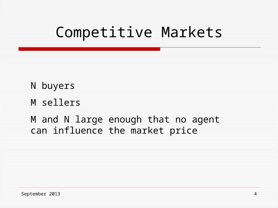
The market demand function tells us how Qd (the quantity of a good demanded by the sum of all consumers in the market) depends on various factors
Qd
=
Q(p,po,I,…)
The demand curve plots the aggregate quantity of a good that consumers are willing to buy at different prices, holding constant other demand drivers such as prices of other goods, consumer income, and quality
Qd= Q(p)
The Market Demand Function
The Demand Curve
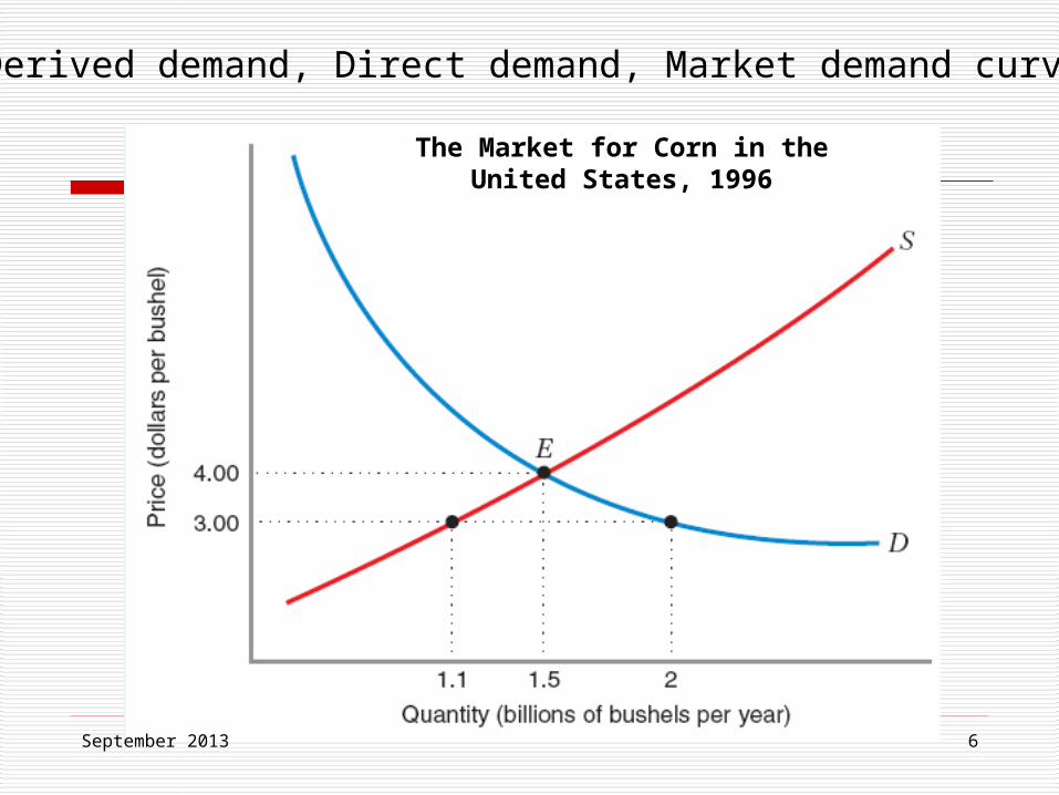
September 2013 6
The Market for Corn in theUnited States, 1996
Derived demand, Direct demand, Market demand curve
September 2013 7
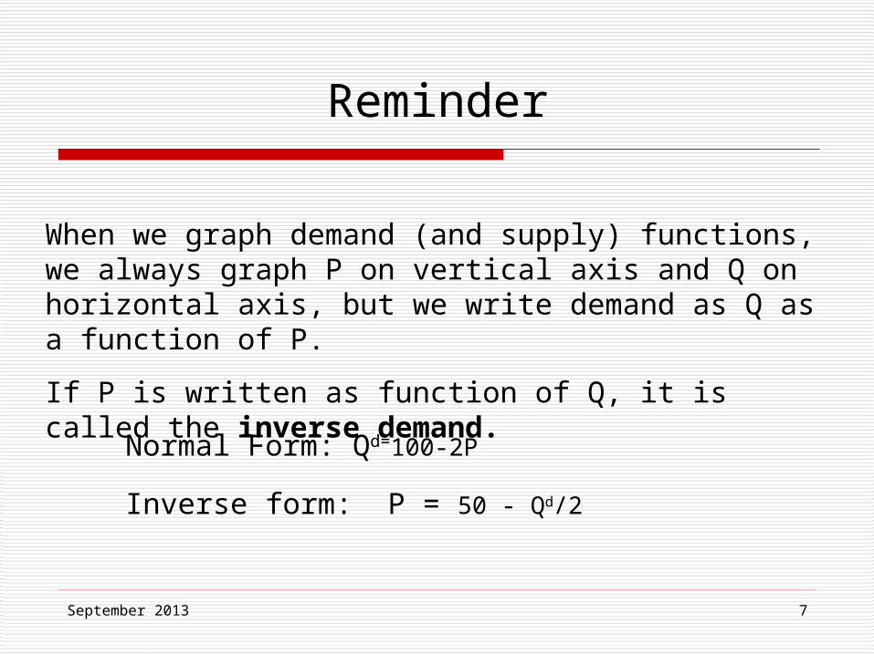
When we graph demand (and supply) functions, we always graph P on vertical axis and Q on horizontal axis, but we write demand as Q as a function of P.
If P is written as function of Q, it is called the inverse demand.
Normal Form: Qd=100-2P
Inverse form: P = 50 - Qd/2
Reminder
September 2013 8
The Law of Demand states that the quantity of a good demanded decreases when the price of this good rises
If the change increases the willingness of consumers to acquire the good, the demand curve shifts right
If the change decreases the willingness of consumers to acquire the good, the demand curve shifts left
The demand curve shifts when factors other than own price change:
The Law of Demand
September 2013 9
A move along the demand curve for a good can only be triggered by a change in the price of that good.
Any change in another factor that affects the consumers’ willingness to pay for the good results in a shift in the demand curve for the good.
Rule
September 2013 10
The market supply function tells us how the quantity of a good supplied by the sum of all producers in the market depends on various factors
Qs=Q(p,po, W, …)
The market supply curve plots the aggregate quantity of a good that will be offered for sale at different prices
Qs= Q(P)
The Market Supply Function
The Market Supply Curve
September 2013 11
Definition: The Law of Supply states that the quantity of a good offered increases when the price of this good increases.
The supply curve shifts when factors other than own price change:If the change increases the willingness of
producers to offer the good at the same price, the supply curve shifts right
If the change decreases the willingness of producers to offer the good at the same price, the supply curve shifts left
The Law of Supply
September 2013 12
A move along the supply curve for a good can only be triggered by a change in the price of that good.
Any change in another factor that affects the producers’ willingness to offer for the good results in a shift in the supply curve for the good.
Rule
September 2013 13
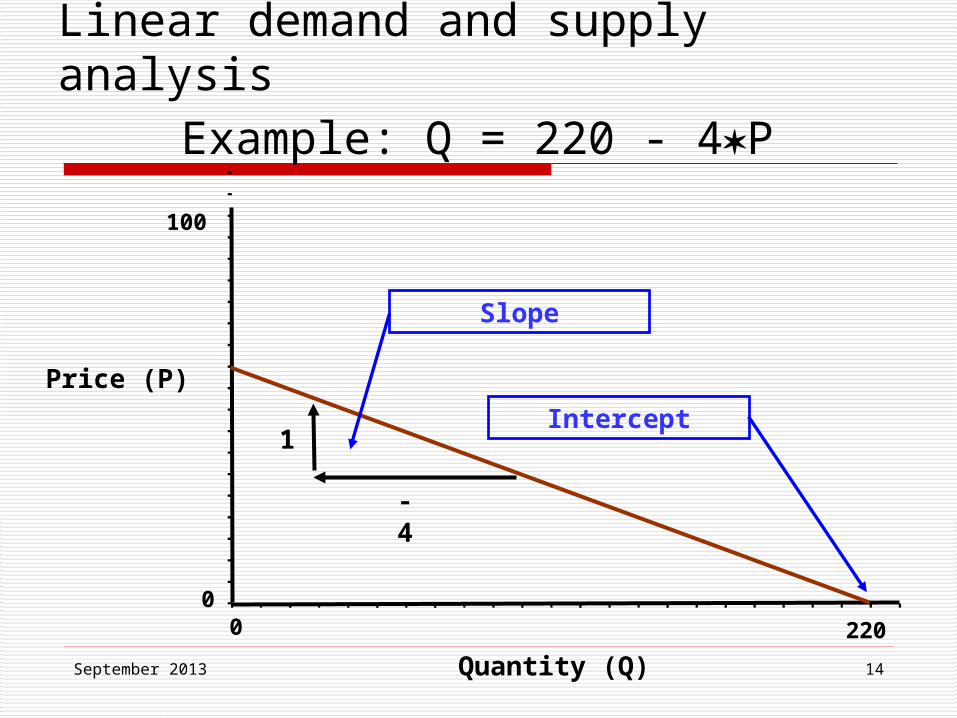
Linear demand and supply analysis
Linear demand and supply curves can be expressed as equations with an intercept and a slope:
Q = I + S P
Q = QuantityI = InterceptS = Slope
September 2013 14
Linear demand and supply analysis
0
100
0 220
Price (P)
Quantity (Q)
Example: Q = 220 - 4P
Intercept
Slope
1
- 4
September 2013 15
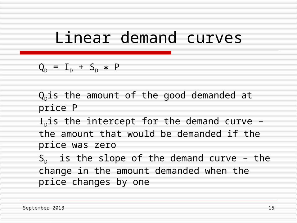
Linear demand curves
QD = ID + SD P
QD is the amount of the good demanded at price P IDis the intercept for the demand curve – the amount that would be demanded if the price was zeroSD is the slope of the demand curve – the change in the amount demanded when the price changes by one
September 2013 16
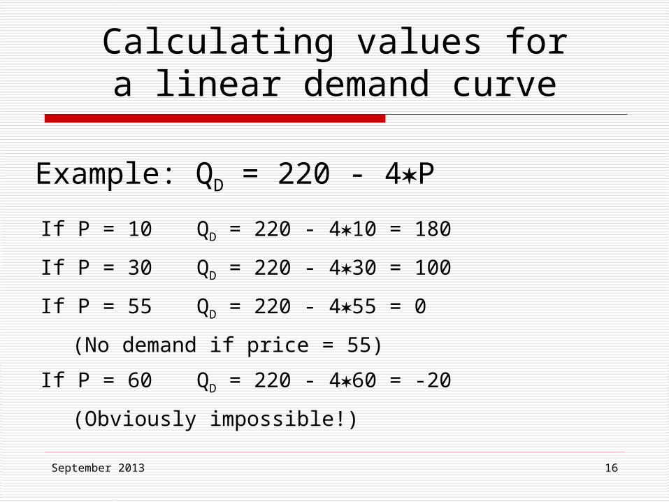
Calculating values fora linear demand curve
If P = 10 QD = 220 - 410 = 180
If P = 30 QD = 220 - 430 = 100
If P = 55 QD = 220 - 455 = 0
(No demand if price = 55)
If P = 60 QD = 220 - 460 = -20
(Obviously impossible!)
Example: QD = 220 - 4P
September 2013 17
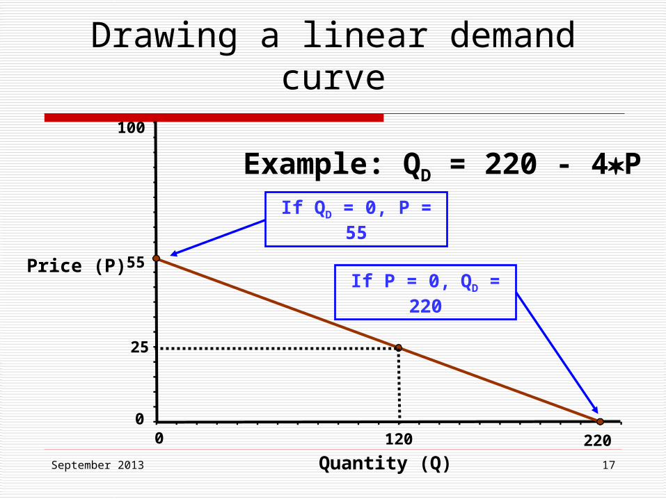
Drawing a linear demand curve
0
25
55
100
0 220
Price (P)
Quantity (Q)120
Example: QD = 220 - 4P
If P = 0, QD = 220
If QD = 0, P = 55
September 2013 18
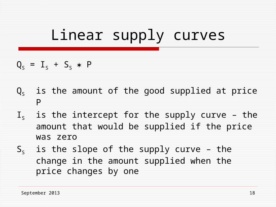
Linear supply curves
QS = IS + SS P
QS is the amount of the good supplied at price P
IS is the intercept for the supply curve – the amount that would be supplied if the price was zero
SS is the slope of the supply curve – the change in the amount supplied when the price changes by one
September 2013 19
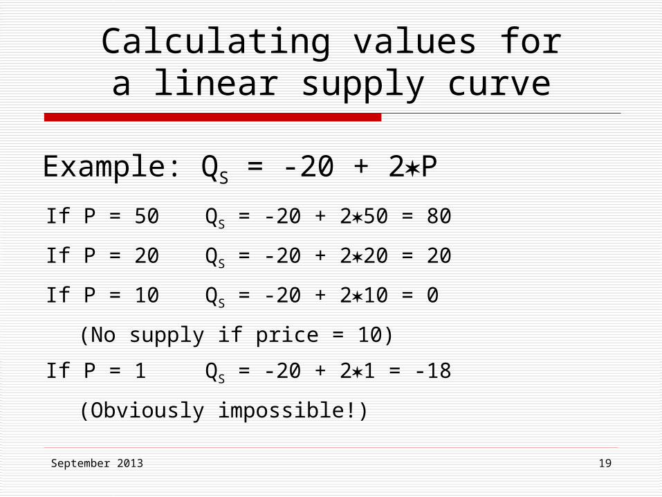
Calculating values fora linear supply curve
If P = 50 QS = -20 + 250 = 80
If P = 20 QS = -20 + 220 = 20
If P = 10 QS = -20 + 210 = 0
(No supply if price = 10)
If P = 1 QS = -20 + 21 = -18
(Obviously impossible!)
Example: QS = -20 + 2P
September 2013 20
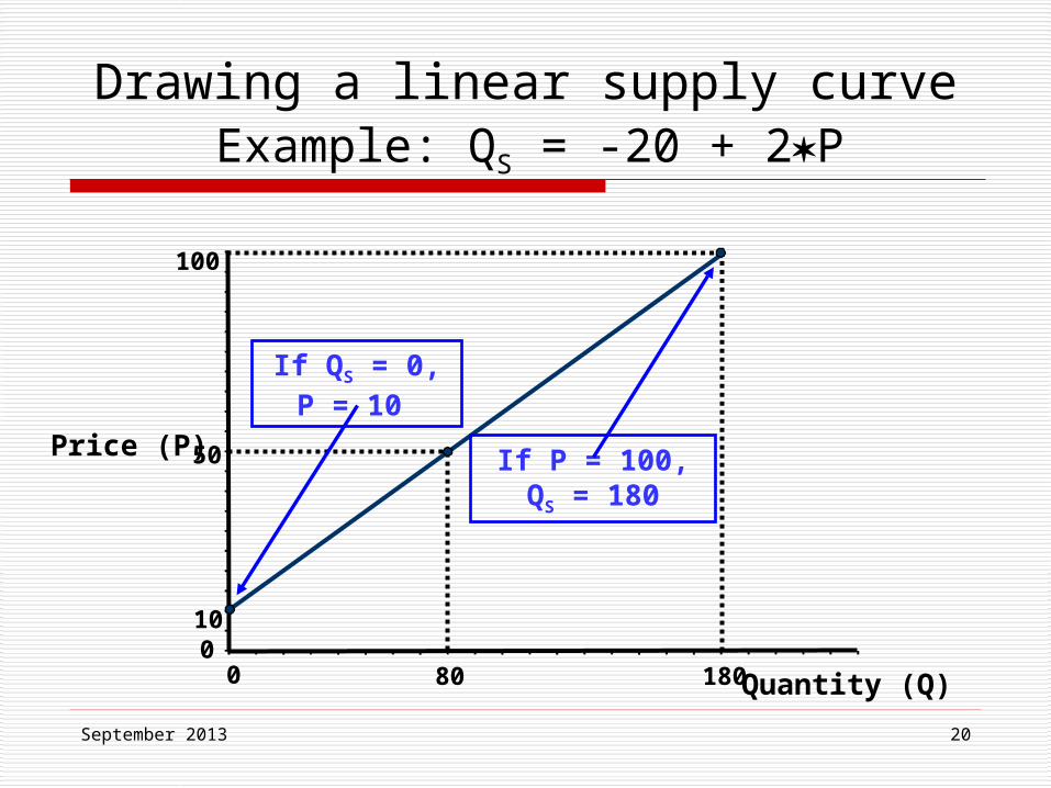
Drawing a linear supply curveExample: QS = -20 + 2P
Quantity (Q)010
50
100
0
Price (P)
80 180
If QS = 0, P = 10
If P = 100, QS = 180
September 2013 21
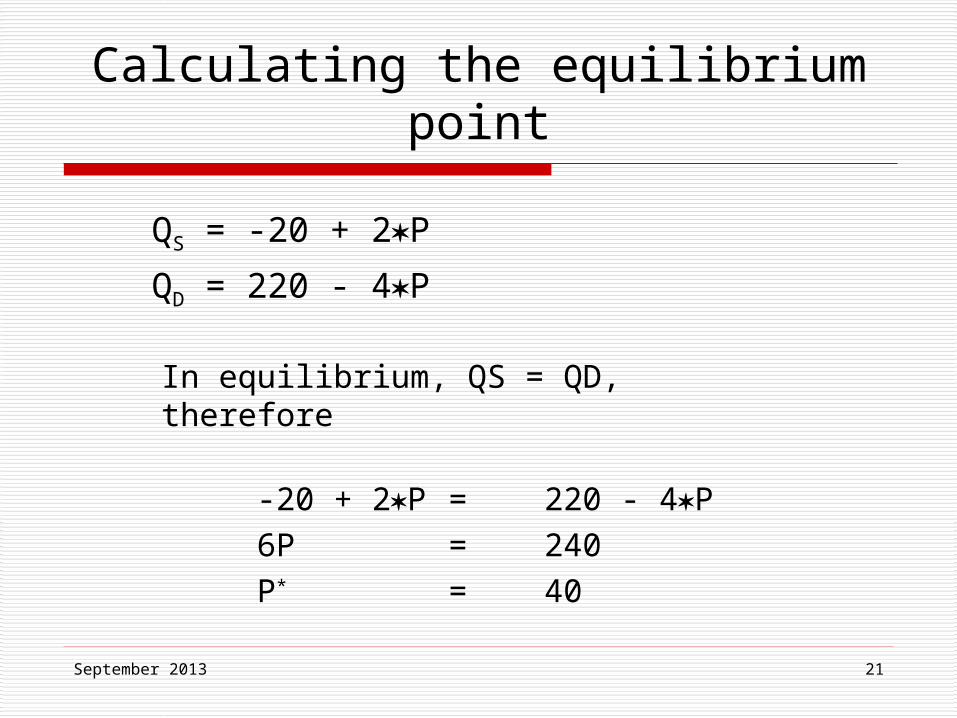
QS = -20 + 2P
QD = 220 - 4P
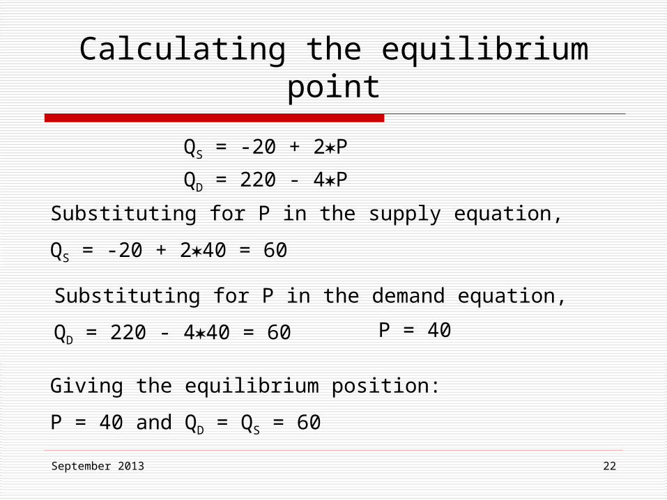
Calculating the equilibrium point
In equilibrium, QS = QD, therefore
-20 + 2P = 220 - 4P6P = 240P* = 40
September 2013 22
Calculating the equilibrium point
Substituting for P in the supply equation,
QS = -20 + 240 = 60
Substituting for P in the demand equation,
QD = 220 - 440 = 60
Giving the equilibrium position:
P = 40 and QD = QS = 60
P = 40
QS = -20 + 2P
QD = 220 - 4P
September 2013 23
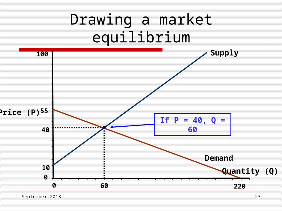
Drawing a market equilibrium
0
10
40
55
100
0 220
Supply
Demand
Price (P)
60
Quantity (Q)
If P = 40, Q = 60
September 2013 24
0
55
0 220
Price (P)
Quantity (Q)
10
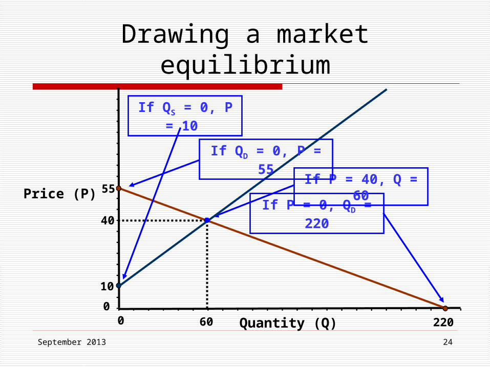
If P = 0, QD = 22040
If P = 40, Q = 60
60
If QS = 0, P = 10
If QD = 0, P = 55
Drawing a market equilibrium
September 2013 25
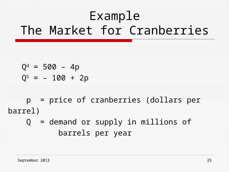
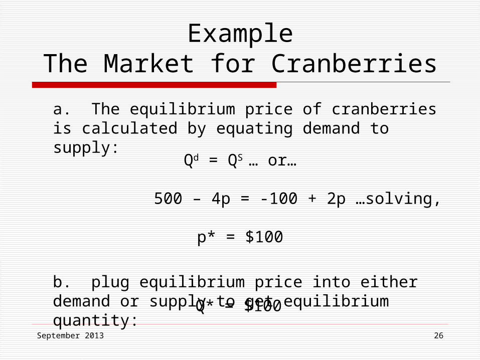
Qd = 500 – 4p QS = – 100 + 2p
p = price of cranberries (dollars per barrel) Q = demand or supply in millions of barrels per year
ExampleThe Market for Cranberries
September 2013 26
a. The equilibrium price of cranberries is calculated by equating demand to supply:
b. plug equilibrium price into either demand or supply to get equilibrium quantity:
Qd = QS … or…
500 – 4p = -100 + 2p …solving,
p* = $100
ExampleThe Market for Cranberries
Q* = $100
September 2013 27
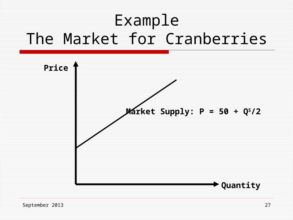
Price
Quantity
Market Supply: P = 50 + QS/2
ExampleThe Market for Cranberries
September 2013 28
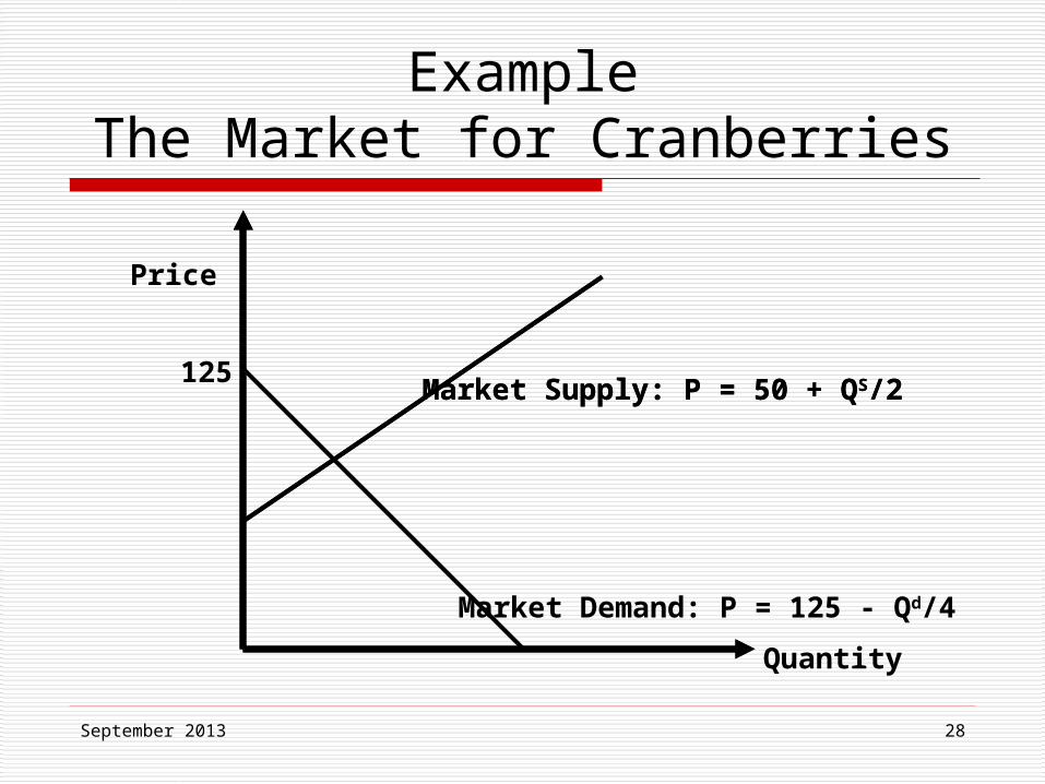
Market Supply: P = 50 + QS/2
Price
Quantity
Market Demand: P = 125 - Qd/4
Market Supply: P = 50 + QS/2125
ExampleThe Market for Cranberries
September 2013 29
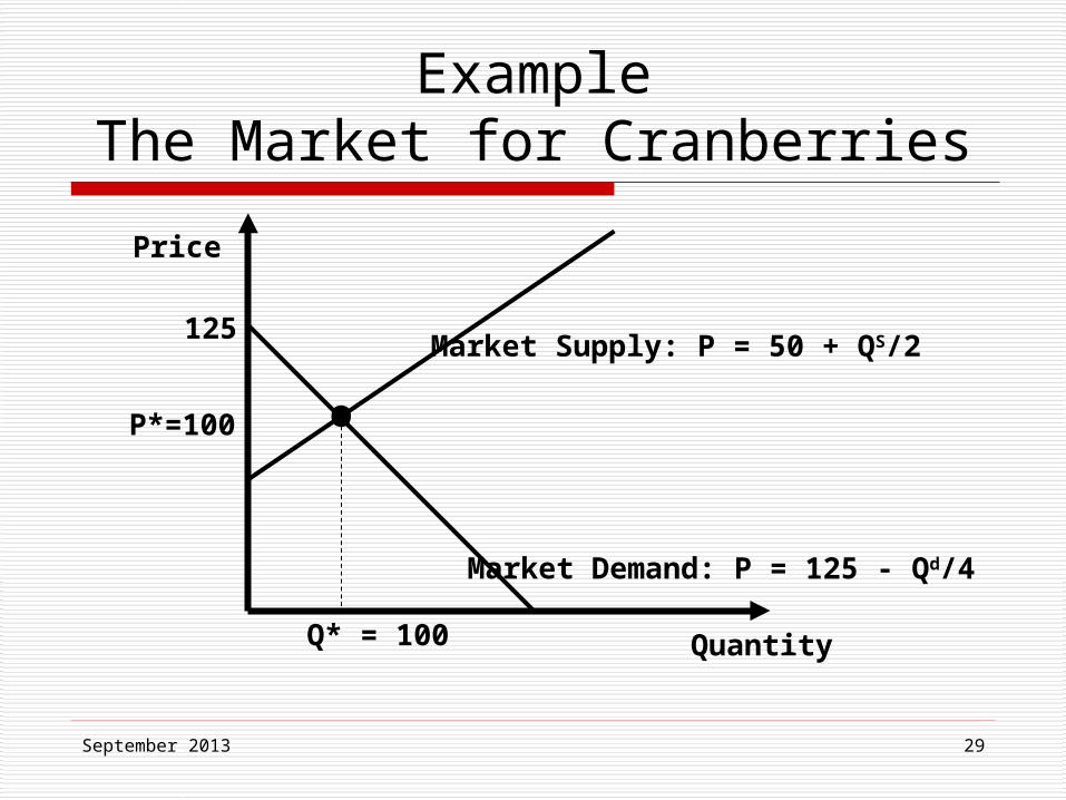
Price
Quantity
Market Demand: P = 125 - Qd/4
Market Supply: P = 50 + QS/2
Q* = 100
P*=100
125
•
ExampleThe Market for Cranberries
September 2013 30
Definition: If sellers cannot sell as much as they would like at the current price, there is excess supply or surplus
ExampleThe Market for Cranberries
September 2013 31
Price
Quantity
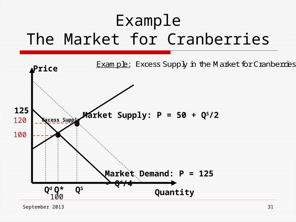
Market Demand: P = 125 - Qd/4
Market Supply: P = 50 + QS/2
Q*
125Excess Supply
••
QSQd
Example: Excess Supply in the Market for Cranberries
ExampleThe Market for Cranberries
120
100
100
September 2013 32
Price
Quantity
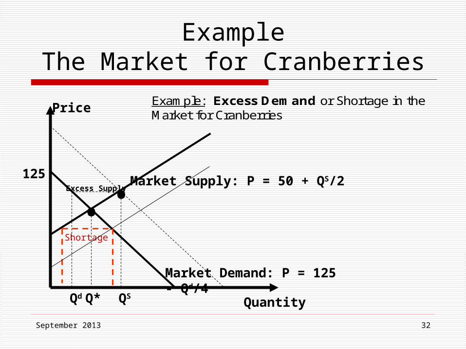
Market Demand: P = 125 - Qd/4
Market Supply: P = 50 + QS/2
Q*
125Excess Supply
••
QSQd
Example: Excess Demand or Shortage in the Market for Cranberries
ExampleThe Market for Cranberries
Shortage
September 2013 33
If there is no excess supply or excess demand, there is no pressure for prices to change and we are in equilibrium.
When a change in an exogenous variable causes the demand curve or the supply curve to shift, the equilibrium shifts as well.
Excess Supply
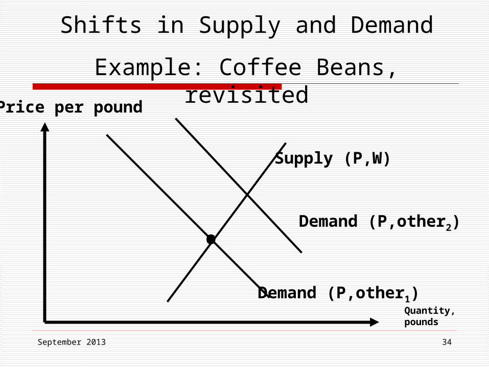
September 2013 34
Price per pound
Quantity, pounds
Demand (P,other2)
Demand (P,other1)
Supply (P,W)
•
Shifts in Supply and Demand
Example: Coffee Beans, revisited
September 2013 35
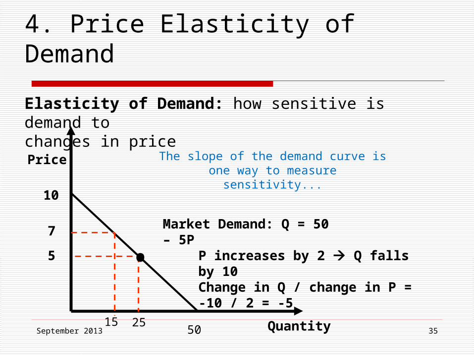
4. Price Elasticity of Demand
Elasticity of Demand: how sensitive is demand tochanges in price
Price
Quantity
Market Demand: Q = 50 – 5P
10
50
7
5
15 25
P increases by 2 Q falls by 10Change in Q / change in P = -10 / 2 = -5
The slope of the demand curve isone way to measure sensitivity...
•
September 2013 36
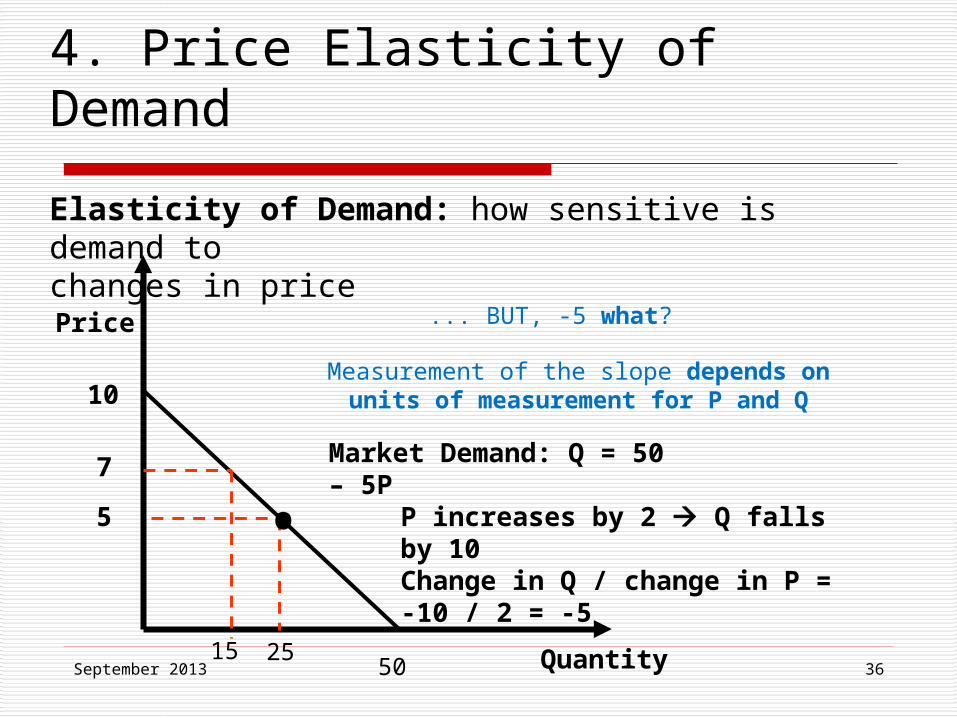
4. Price Elasticity of Demand
Elasticity of Demand: how sensitive is demand tochanges in price
Price
Quantity
Market Demand: Q = 50 – 5P
10
50
7
5
15 25
P increases by 2 Q falls by 10Change in Q / change in P = -10 / 2 = -5
... BUT, -5 what?
Measurement of the slope depends onunits of measurement for P and Q
•
September 2013 37
4. Price Elasticity of Demand
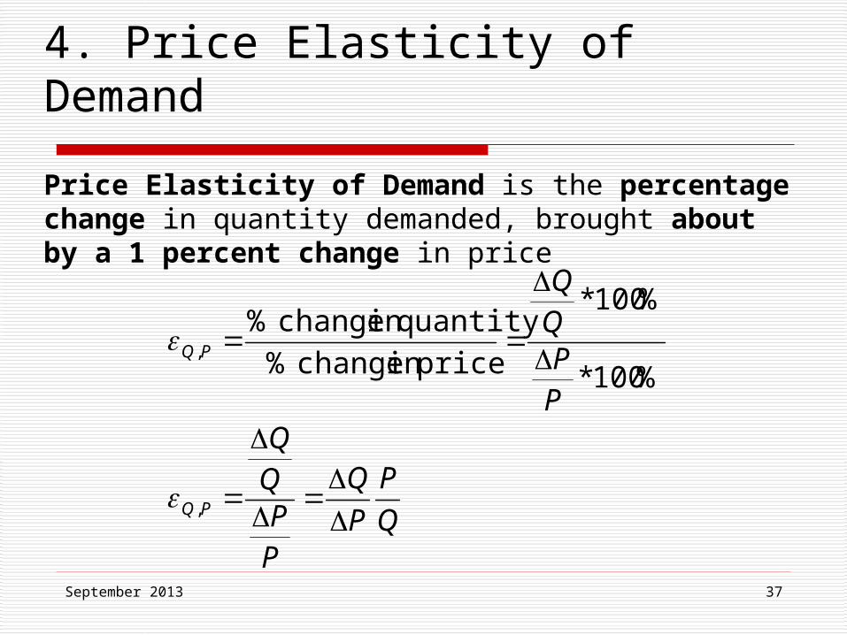
Price Elasticity of Demand is the percentage change in quantity demanded, brought about by a 1 percent change in price
Q
P
P
Q
PPQQ
PPQQ
PQ
PQ
,
,
%100*
%100*
pricein change %
quantityin change %
September 2013 38
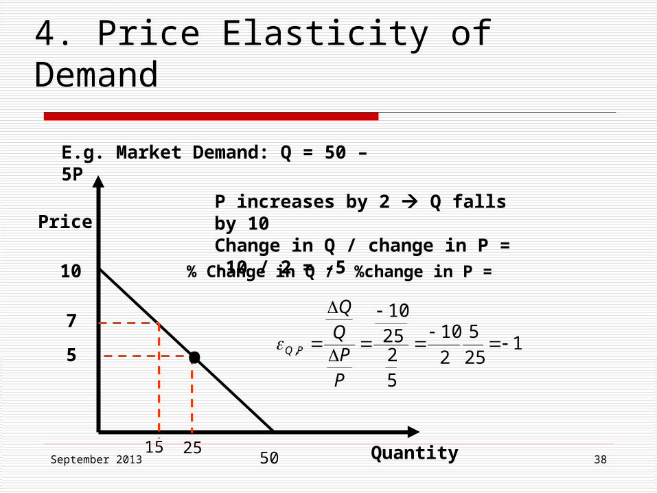
4. Price Elasticity of Demand
Price
Quantity
E.g. Market Demand: Q = 50 – 5P
10
50
7
5
15 25
P increases by 2 Q falls by 10Change in Q / change in P = -10 / 2 = -5
% Change in Q / %change in P =
125
5
2
10
522510
,
PPQQ
PQ•
September 2013 39
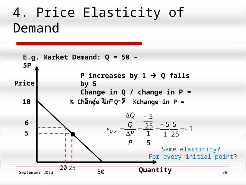
4. Price Elasticity of Demand
Price
Quantity
E.g. Market Demand: Q = 50 – 5P
10
50
6
5
20 25
P increases by 1 Q falls by 5Change in Q / change in P = -5 / 1 = -5
% Change in Q / %change in P =
125
5
1
5
5125
5
,
PPQQ
PQ•Same elasticity?
For every initial point?

September 2013 40
4. Price Elasticity of Demand
Price
Quantity
E.g. Market Demand: Q = 50 – 5P
10
50
6
5
20 25
P falls by 1 Q increases by 5Change in Q / change in P = 5 / -1 = -5
% Change in Q / %change in P =
5.120
6
1
5
61
205
,
PPQQ
PQ•
NO!

September 2013 41
4. Price Elasticity of Demand
Price
Quantity
E.g. Market Demand: Q = 50 – 5P
10
50
6
4
20 30
P falls by 2 Q increases by 10Change in Q / change in P = 10 / -2 = -5
% Change in Q / %change in P =
5.120
6
2
10
62
2010
,
PPQQ
PQ•Will this happen for every
demand function?

September 2013 42
Example

September 2013 43
Example
Comparing the price-elasticity of demand on different demand curves

September 2013 44
Example

September 2013 45
4. Price Elasticity of Demand

September 2013 46
4. Price Elasticity of Demand (intuition)
• When demand is elastic, increase in q offsets the fall in price, increasing revenue.
• When demand is inelastic, increase in p offsets the fall in q, increasing revenue.
• When demand is unit-elastic, revenue is maximum.
Note: Revenue = Consumer Expenditure = P*Q

September 2013 47
Category Estimated Q,P
Soft Drinks -3.18
Canned Seafood -1.79
Canned Soup -1.62
Cookies -1.6
Breakfast Cereal -0.2
Toilet Paper -2.42
Laundry Detergent
-1.58
Toothpaste -0.45
Snack Crackers -0.86
Cigarretes -0.10
Paper Towels -0.05
Dish Detergent -0.74
Fabric Softener -0.73
Price Elasticity of Demand for Selected Products, Chicago, 1990s
4. Price Elasticity of Demand

September 2013 48
4. More Elasticities
* Income Elasticity of demand is the percentage change in quantity demanded, brought about by a 1 percent change in income
Q
I
I
Q
IIQQ
IIQQ
IQ
IQ
,
,
%100*
%100*
incomein change %
quantityin change %

September 2013 49
4. More Elasticities
* Cross-Price Elasticity of demand is the percentage change in quantity of good i demanded, brought about by a 1 percent change of the price of good j.
i
j
j
i
j
j
i
i
IQ Q
P
P
Q
P
PQQ
, > 0 then...
< 0 then...


![Auctions with Resale Opportunities: An Experimental StudyMore recently, Georganas [4] and Jabs-Saral [12] have studied English auctions with resale using experiments. While Georganas](https://img.pdfslide.net/doc/110x75/60d28e1285c227190248211b/auctions-with-resale-opportunities-an-experimental-more-recently-georganas-4.jpg)