Embed Size (px)
Citation preview

Microlocal analysis of a spindle transform
James Webber∗ Sean Holman†
Abstract
An analysis of the stability of the spindle transform, introduced in [1], ispresented. We do this via a microlocal approach and show that the normaloperator for the spindle transform is a type of paired Lagrangian operator with“blowdown–blowdown” singularities analogous to that of a limited data syn-thetic aperture radar (SAR) problem studied by Felea et. al. [2]. We find thatthe normal operator for the spindle transform belongs to a class of distibutionsIp,l(∆ ∪ ∆,Λ) studied by Felea and Marhuenda in [2, 3], where ∆ is reflectionthrough the origin, and Λ is associated to a rotation artefact. Later, we derivea filter to reduce the strength of the image artefact and show that it is of con-volution type. We also provide simulated reconstructions to show the artefactsproduced by Λ and show how the filter we derived can be applied to reduce thestrength of the artefact.
1 Introduction
Here we present a microlocal analysis of the spindle transform, first introduced by theauthors in [1], which describes the Compton scattering tomography problem in threedimensions for a monochromatic source and energy sensitive detector pair. Comptonscattering is the process in which a photon interacts in an inelastic collision with acharged particle. As the collision is inelastic, the photon undergoes a loss in energy,described by the equation
Es =Eλ
1 + (Eλ/E0) (1− cosω), (1)
where Es is the energy of the scattered photon which had an initial energy Eλ, ω isthe scattering angle and E0 ≈ 511keV is the electron rest energy. For Es and Eλfixed (i.e if the source is monochromatic and we can measure Es), the scattering angleω remains fixed and, in three dimensions, the surface of scatterers is the surface ofrevolution of a circular arc [1]. The surface of revolution of a circular arc is a spindletorus. We define
Tr =
(x1, x2, x3) ∈ R3 :
(r −
√x2
1 + x22
)2
+ x23 = 1 + r2
(2)
∗Corresponding author, supported by Engineering and Physical Sciences Research Council andRapiscan systems, CASE studentship.†Second author supported by Engineering and Physical Sciences Research Council
(EP/M016773/1).
1
arX
iv:1
706.
0316
8v1
[m
ath.
FA]
10
Jun
2017

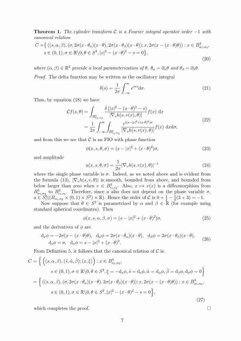
to be the spindle torus, radially symmetric about the x3 axis, with tube centre offsetr ≥ 0 and tube radius
√1 + r2. See figure 1 which displays a rotation of Tr.
In [12] Norton considered the problem of reconstructing a density supported in aquadrant of the plane from the Compton scattered intensity measured at a single pointdetector moved laterally along the axis away from a point source at the origin. Herethe curve of scatterers is a circle. He considers the circle transform
Af(r, φ) =
∫ π2
−π2
rF (r cosϕ, ϕ+ φ)dϕ, (3)
where F (ρ, θ) = f(ρ cos θ, ρ sin θ) is the polar form of f : R2 → R. Let f(x) =1|x|2 f( x
|x|2 ). Then Af(r, φ) = Rf(1r, φ), where R denotes the polar form of the straight
line Radon transform. So A is equivalent to R via the diffeomorphism x → x|x|2 and
from this we can derive stability estimates from known theory on the Radon transform[13].
In [10, 11], Nguyen and Truong consider an acquisition geometry of a point sourceand detector which remain opposite one another and are rotated on S1, and aim toreconstruct a density supported on the unit disc. Here the curve of scatterers is acircular arc. They define the circular arc transform
Bf(r, φ) =
∫ π2
−π2
ρ
√1 + r2
1 + r2 cos2 ϕF (ρ, ϕ+ φ) |
ρ=√r2 cos2 ϕ+1−r cosϕ
dϕ. (4)
Letting f(x) =
√|x|2+1−|x|1−|x|2 f
((√|x|2 + 1− |x|
)· x|x|)
, we have that r√1+r2
Bf(r, φ) =
Af(r, φ), and henceB is equivalent toA via the diffeomorphism x→(√|x|2 + 1− |x|
)x|x| .
So, in two dimensions, the inverse problem for Compton scattering tomography is in-jective and mildly ill posed (the solution is bounded in some Sobolev space). In [10],Palamodov also derives stability estimates for a more general class of Minkowski–Funktransforms.
In [1] the authors consider a three dimensional acquisition geometry, where a singlesource and detector are rotated opposite one another on S2 and a density supportedon a hollow ball is to be recovered. Here the surface of scatterers is a spindle torus.They define the spindle transform
Sf(r, θ) =
∫ 2π
0
∫ π
0
ρ2 sinϕ
√1 + r2
1 + r2 sin2 ϕ(h · F ) (ρ, ψ, ϕ) |
ρ=√r2 sin2 ϕ+1−r sinϕ
dϕdψ,
(5)where F (ρ, ψ, ϕ) = f(ρ cosψ sinϕ, ρ sinψ sinϕ, ρ cosϕ) is the spherical polar form off : R3 → R and h ∈ SO(3) describes the rotation of the north pole to θ, where hdefines a group action on real-valued functions in the natural way (h · f)(x) = f(hx).They show that a left inverse to S exists through the explicit inversion of a set of one-dimensional Volterra integral operators, and show that the null space of S consists ofthose functions whose even harmonic components are zero (odd functions). Howeverthe stability of the spindle transform was not considered. We aim to address this herefrom a microlocal perspective. In [2], various acquisition geometries are consideredfor synthetic aperture radar imaging of moving objects. In each case the microlocalproperties of the forward operator in question and its normal operator are analysed. In
2

x
θ
r
√1 + r2
x3
x1
Figure 1: A spindle torus with axis of rotation θ, tube centre offset r and tube radius√1 + r2. The distance between the origin and either of the points where the torus self
intersects is 1.
three of the four cases considered the Schwartz kernel of the normal operator was shownto belong to a class of distributions associated to two cleanly intersecting LagrangiansIp,l(∆,Λ) (that is, the wavefront set of the kernel of the normal operator is contained in∆∪Λ). We show a similar result for the spindle transform S∗S, although the diagonal
∆ is replaced by the disjoint union ∆∪ ∆ where ∆ is reflection through the origin. Wealso determine the associated Lagrangian Λ. In [2] they suggest a way to reduce thesize of the image artefact microlocally by applying an appropriate pseudodifferentialoperator as a filter before applying the backprojection operator. Similarly we derivea suitable filter for the spindle transform and show how it can be applied using thespherical harmonics of the data.
In section 2.1 we show that S is equivalent to a weighted cylinder transform C,which gives the weighted integrals over cylinders with an axis of revolution throughthe origin. After this we prove that C is a Fourier integral operator and determineits canonical relation. Later in section 2.2 we present our main theorem (Theorem 3),
where we show that C belongs to a class of distributions Ip,l(∆ ∪ ∆,Λ), where ∆ is areflection and the Lagrangian Λ is associated to a rotation artefact.
3

In section 3, we adopt the ideas of Felea et al in [2] and derive a suitable pseudodif-ferential operator Q which, when applied as a filter before applying the backprojectionoperator of the cylinder transform, reduces the artefact intensity in the image. Weshow that Q can be applied by multiplying the harmonic components of the databy a factor cl, which depends on the degree l of the component, and show how thistranslates to a spherical convolution of the data with a distribution on the sphere h.
Simulated reconstructions from spindle transform data are presented in section4. We reconstruct a small bead of constant density by unfiltered backprojection andshow the artefacts produced by Λ in our reconstruction. We then reconstruct thesame density by filtered backprojection, applying the filter Q as an intermediate step,and show how the size of the artefacts are reduced in the image. Later we providereconstructions of densities of oscillating layers using the conjugate gradient leastsquares (CGLS) method and Landweber iteration. We arrange the layers as sphericalshells centred at the origin and as planes and compare our results. We also investigatethe effects of applying the filter Q as a pre–conditioner, prior to implementing CGLSand the Landweber method.
2 The microlocal properties of S and S∗SHere we investigate the microlocal properties of the spindle transform and its normaloperator. We start by showing the equivalence of S to a cylinder transform C, and howwe can write S and C as Fourier integral operators. Then we determine the canonicalrelations associated with C and from these we discover that C∗C is a paired Lagrangianoperator with blowdown–blowdown singularities. First we give some preliminaries.
Let Bnε1,ε2
= x ∈ Rn : 0 < ε1 < |x| < ε2 < 1 denote the set of points on a hollowball with inner radius ε1 and outer radius ε2. Let Zn = R×Sn−1 denote the n–cylinderand, for X ⊂ Rn an open set, let D′(X) denote the vector space of distributions on X,and let E ′(X) denote the vector space of distributions with compact support containedin X.
Definition 1. For a function f in the Schwarz space S(Rn) we define the Fouriertransform and its inverse in terms of angular frequency as
Ff(ξ) = (2π)−n2
∫Rne−ix·ξf(x)dx,
F−1f(x) = (2π)−n2
∫Rneix·ξf(ξ)dξ.
(6)
Definition 2. Let m, ρ, δ ∈ R with 0 ≤ ρ ≤ 1 and δ = 1 − ρ. Then we defineSmρ (X×Rn) to be the set of a ∈ C∞(X×Rn) such that for every compact set K ⊂ Xand all multi–indices α, β the bound∣∣∂βx∂αξ a(x, ξ)
∣∣ ≤ Cα,β,K(1 + |ξ|)m−ρ|α|+δ|β|, x ∈ K, ξ ∈ Rn, (7)
holds for some constant Cα,β,K . The elements of Smρ are called symbols of order m,type ρ.
Definition 3. A function φ = φ(x, ξ) ∈ C∞(X × RN\0) is a phase function ifφ(x, λξ) = λφ(x, ξ), ∀λ > 0 and dφ 6= 0.
4

Definition 4. Let X ⊂ Rnx , Y ∈⊂ Rny be open sets. A Fourier integral operator(FIO) of order m + N/2 − (nx + ny)/4 is an operator A : C∞0 (X) → D′(Y ) withSchwartz kernel given by an oscillatory integral of the form
Af(y) =
∫RNeiφ(x,y,ξ)a(x, y, ξ)dξ, (8)
where φ is a phase function, and a ∈ Smρ ((X × Y )× RN) is a symbol.
Definition 5. The canonical relation of an FIO with phase function φ is defined as
C =((y, η), (x, ω)) ∈(Y × RN\0
)×(X × RN\0
): (x, y, ω) ∈ Σφ,
ω = −dxφ(x, y, ξ), η = dyφ(x, y, ξ), ω, η 6= 0,(9)
where Σφ = (x, ξ) ∈ X × RN\0 : dξφ = 0 is the critical set of φ.
If Y and X are manifolds without boundary, then an operator A : C∞0 (X)→ D′(Y ) isa Fourier integral operator if its Schwartz kernel can be represented locally in coordi-nates by oscillatory integrals of the form (8), and the canonical relations of the phasefunctions for the local representations all lie within a single immersed Lagrangian sub-manifold of T ∗Y ×T ∗X. For much more detail on Fourier integral operators and theirdefinition see [4].
2.1 The spindle transform as an FIO
Recall the author’s acquisition geometry in [1] (displayed in figure 1). We have theimplicit equation
(r + |x× θ|)2 + (x · θ)2 = 1 + r2 (10)
for the set of points on a spindle with tube centre offset r and axis of revolution givenby θ ∈ S2. With this in mind we define
h(s, x, θ) =4|x× θ|2
(1− |x|2)2− s, (11)
and then we can write the spindle transform S : C∞0 (B3ε1,ε2
)→ C∞((0, 1)× S2) as
Sf(s, θ) =
∫B3ε1,ε2
δ(
4|x×θ|2(1−|x|2)2
− s)
|∇xh(s, x, θ)|f(x)dx, (12)
where s = 1/r2 and δ is the Dirac–delta function. Note that
∇xh(s, x, θ) = 8(x− (x · θ)θ)
(1− |x|2)2+ 16
|x× θ|2x(1− |x|2)3
(13)
is smooth, bounded above, and does not vanish on on (0, 1) × B3ε1,ε2× S2. We define
the backprojection operator S∗ : C∞((0, 1)× S2)→ C∞(B3ε1,ε2
) as
S∗g(x) =
∫S2
g(
4|x×θ|2(1−|x|2)2
, θ)
|∇xh(s, x, θ)|dΩ, (14)
where dΩ is the surface measure on S2.
5

Proposition 1. The backprojection operator S∗ is the adjoint operator to S.
Proof. Let g ∈ C∞((0, 1)×S2) and f ∈ C∞0 (B3ε1,ε2
). Then (in the third step note that∇xh does not actually depend on s)
〈g,Sf〉 =
∫S2
∫ 1
0
g(s, θ)Sf(s, θ)dsdΩ
=
∫S2
∫ 1
0
g(s, θ)
∫B3ε1,ε2
δ(
4|x×θ|2(1−|x|2)2
− s)
|∇xh(s, x, θ)|f(x)dxdsdΩ
=
∫B3ε1,ε2
∫S2
g(
4|x×θ|2(1−|x|2)2
, θ)
|∇xh(s, x, θ)|dΩf(x)dx
=
∫B3ε1,ε2
S∗g(x)f(x)dx = 〈S∗g, f〉,
(15)
which completes the proof.
Let v(x) =(√
1 + 1|x|2 −
1|x|
)· x|x| , and set αi = 2εi/(1 − ε2i ) for i = 1 or 2 so that
when |x| = αi, |v(x)| = εi. Then, after making the substitution x→ v(x) in equation(12), we have
Sf(s, θ) =
∫B3α1,α2
|det(Jv)|δ (|x× θ|2 − s)|∇vh(s, v(x), θ)|
f
((√1 +
1
|x|2− 1
|x|
)· x|x|
)dx
=
∫B3α1,α2
δ (|x|2 − (x · θ)2 − s)|∇vh(s, v(x), θ)|
f(x)dx,
(16)
where
f(x) = |det(Jv)| f
((√1 +
1
|x|2− 1
|x|
)· x|x|
). (17)
We define the weighted cylinder transform C : C∞0 (B3α1,α2
)→ C∞((0, 1)× S2) as
Cf(s, θ) =
∫B3α1,α2
δ (|x|2 − (x · θ)2 − s)√|∇vh(s, v(x), θ)|
f(x)dx (18)
and its backprojection operator C∗ : C∞((0, 1)× S2)→ C∞(B3α1,α2
):
C∗g(x) =
∫S2
g (|x× θ|2, θ)|∇vh(s, v(x), θ)|
dΩ. (19)
As in Proposition 1, we can show that C∗ is the formal adjoint to C.The above is to say that the spindle transform is equivalent, via the diffeomorphism
x →(√
1 + 1|x|2 −
1|x|
)· x|x| , to the transform C which defines the weighted integrals
over cylinders with radius√s and axis of rotation through the origin with direction
θ. With this in mind we consider the microlocal properties of the cylinder transformC and its normal operator C∗C for the remainder of this section.
First, we characterise C as a Fourier integral operator in the next theorem.
6
Theorem 1. The cylinder transform C is a Fourier integral operator order −1 withcanonical relation
C =
((s, α, β), (σ, 2σ(x · θα)(x · θ), 2σ(x · θβ)(x · θ));x, 2σ(x− (x · θ)θ)) : x ∈ B3α1,α2
,
s ∈ (0, 1), σ ∈ R\0, θ ∈ S2, |x|2 − (x · θ)2 − s = 0,
(20)
where (α, β) ∈ R2 provide a local parameterization of θ, θα = ∂αθ and θβ = ∂βθ.
Proof. The delta function may be written as the oscillatory integral
δ(s) =1
2π
∫ ∞−∞
eiσsdσ. (21)
Thus, by equation (18) we have
Cf(s, θ) =
∫B3α1,α2
δ (|x|2 − (x · θ)2 − s)|∇vh(s, v(x), θ)|
f(x) dx
=1
2π
∫ ∞−∞
∫B3α1,α2
ei(s−|x|2+(x·θ)2)σ
|∇vh(s, v(x), θ)|f(x) dxdσ,
(22)
and from this we see that C is an FIO with phase function
φ(x, s, θ, σ) = (s− |x|2 + (x · θ)2)σ, (23)
and amplitude
a(x, s, θ, σ) =1
2π|∇vh(s, v(x), θ)|−1 (24)
where the single phase variable is σ. Indeed, as we noted above and is evident fromthe formula (13), |∇vh(s, v, θ)| is smooth, bounded from above, and bounded frombelow larger than zero when v ∈ B3
ε1,ε2. Also, x 7→ v(x) is a diffeomorphism from
B3α1,α2
to B3ε1,ε2
. Therefore, since a also does not depend on the phase variable σ,a ∈ S0
1((Bα1,α2 × (0, 1)× S2)× R). Hence the order of C is 0 + 12− 1
4(3 + 3) = −1.
Now suppose that θ ∈ S2 is parametrized by α and β ∈ R (for example usingstandard spherical coordinates). Then
φ(x, s, α, β, σ) = (s− |x|2 + (x · θ)2)σ, (25)
and the derivatives of φ are
dxφ = −2σ(x− (x · θ)θ), dαφ = 2σ(x · θα)(x · θ), dβφ = 2σ(x · θβ)(x · θ),dsφ = σ, dσφ = s− |x|2 + (x · θ)2.
(26)
From Definition 5, it follows that the canonical relation of C is:
C =(
(s, α, β), (s, α, β); (x, ξ))
: x ∈ B3α1,α2
,
s ∈ (0, 1), σ ∈ R\0, θ ∈ S2, ξ = −dxφ, s = dsφ, α = dαφ, β = dβφ, dσφ = 0
=
((s, α, β), (σ, 2σ(x · θα)(x · θ), 2σ(x · θβ)(x · θ));x, 2σ(x− (x · θ)θ)) : x ∈ B3α1,α2
,
s ∈ (0, 1), σ ∈ R\0, θ ∈ S2, |x|2 − (x · θ)2 − s = 0,
(27)
which completes the proof.
7
2.2 C∗C as a paired Lagrangian operator
If we analyse the canonical relation C given in Theorem 1, we can see that it is non-injective as the points on the ring x ∈ R3 : |x|2−s = 0, x·θ = 0 map to ((s, θ), (σ, 0))if we fix s and σ. Let C∗ be the canonical relation of C∗ and let ∆ denote the diagonal.Then, given the non-injectivity of C, C∗ C * ∆ and C∗C is not a pseudodifferentialoperator, or even an FIO. In this section we show that the Schwarz kernel of C∗Cinstead belongs to a class of distributions Ip,l(∆ ∪ ∆,Λ) studied in [2, 3]. First werecall some definitions and theorems from [2].
Definition 6. Two submanifolds M,N ⊂ X intersect cleanly if M ∩ N is a smoothsubmanifold and T (M ∩N) = TM ∩ TN
Definition 7. We define Im(C) to be the set of Fourier integral operators, A : E ′(X)→D′(Y ), of order m with canonical relation C ⊂ (T ∗Y \ 0)× (T ∗X \ 0)
Recall the definitions of the left and right projections of a canonical relation.
Definition 8. Let C be the canonical relation associated to the FIO A : E ′(X) →D′(Y ). Then we denote πL and πR to be the left and right projections of C, πL : C →T ∗Y \0 and πR : C → T ∗X\0.
We have the following result from [4].
Proposition 2. Let dim(X) = dim(Y ). Then at any point in C:
(i) if one of πL or πR is a local diffeomorphism, then C is a local canonical graph;
(ii) if one of the projections πR or πL is singular, then so is the other. The type ofthe singularity may be different (e.g. fold or blowdown [6]) but both projectionsdrop rank on the same set
Σ = (y, η;x, ξ) ∈ C : det(dπL) = 0 = (y, η;x, ξ) ∈ C : det(dπR) = 0. (28)
Now we have the definition of a blowdown singularity and the definitions of a nonradialand involutive submanifold:
Definition 9. Let M and N be manifolds of dimension n and let f : N → M bea smooth function. f is said to have a blowdown singularity of order k ∈ N along asmooth hypersurface Σ ⊂ M if f is a local diffeomorphism away from Σ, df dropsrank by k at Σ, ker(df) ⊂ T (Σ), and the determinant of the Jacobian matrix vanishesto order k at Σ.
Definition 10. A submanifold M ⊂ T ∗X is nonradial if ρ /∈ (TM)⊥, where ρ =∑ξi∂ξi .
Definition 11. A submanifold M ⊂ T ∗X, M = (x, ξ) : pi(x, ξ) = 0, 1 ≤ i ≤ k isinvolutive if the differentials dpi, i = 1, . . . , k, are linearly independant and the Poissonbrackets satisfy pi, pj = 0, i 6= j.
From [5], we have the definition of the flowout.
8

Definition 12. Let Γ = (x, ξ) : pi(x, ξ) = 0, 1 ≤ i ≤ k be a submanifold of T ∗X.Then the flowout of Γ is given by (x, ξ; y, η) ∈ T ∗X × T ∗X : (x, ξ) ∈ Γ, (y, η) =exp(
∑ki=1 tiHpi)(x, ξ), t ∈ Rk, where Hpi is the Hamiltonian vector field of pi.
We now state a result of [3, Theorem 1.2] concerning the composition of FIO’s withblowdown–blowdown singularities.
Theorem 2. Let C ⊂ (T ∗Y \0) × (T ∗X\0) be a canonical relation which satifies thefollowing:
(i) away from a hypersurface Σ ⊂ C, the left and right projections πL and πR arediffeomorphisms;
(ii) at Σ, both πL and πR have blowdown singularities;
(iii) πL(Σ) and πR(Σ) are nonradial and involutive.
If A ∈ Im(C) and B ∈ Im′(Ct), then BA ∈ Im+m′+ k−1
2,− k−1
2 (∆,ΛπR(Σ)), where ∆ isthe diagonal and ΛπR(Σ) is the flowout of of πR(Σ).
Finally, for two cleanly intersecting Lagrangians Λ0 and Λ1, we define the Ip,l(Λ0,Λ1)classes as in [2, 7].
We now have our main Theorem.
Theorem 3. Let C be the canonical relation of the cylinder transform C. Then theleft and right projections of C have singularities along a dimension 1 submanifold Σ,πL(Σ) and πR(Σ) are involutive and nonradial, and C∗C ∈ I−2,0(∆ ∪ ∆,Λ), where ∆
is the diagonal in T ∗B3α1,α2
× T ∗B3α1,α2
, ∆ = (−x,−ξ;x, ξ) : (x, ξ) ∈ T ∗B3α1,α2, and
Λ is the flowout of πR(Σ).
Proof. From Theorem 1 we have the canonical relation of the cylinder transform
C =
((s, α, β), (σ, 2σ(x · θα)(x · θ), 2σ(x · θβ)(x · θ));x, 2σ(x− (x · θ)θ)) : x ∈ B3α1,α2
,
s ∈ (0, 1), σ ∈ R\0, θ ∈ S2, |x|2 − (x · θ)2 − s = 0,
(29)
where α and β parameterize θ ∈ S2. Suppose we use standard spherical coordinatescentred at any given point on S2 (e.g. when centred at (1, 0, 0) these would be definedby θ = (cosα cos β, sinα cos β, sin β)) with the notation
∂αθ = θα, ∂βθ = θβ. (30)
With such a parameterization, θ, θα, θβ is an orthogonal basis for R3 and |θβ| = 1,|θα| = cos β. Furthermore
det
θTθTαθTβ
= cos β. (31)
Using these coordinates on S2, we can also parametrise C by (x, α, β, σ) where x ∈B3α1,α2
is such that |x|2 − (x · θ)2 = (cos β)−2(x · θα)2 + (x · θβ)2 ∈ (0, 1), and (α, β)are in the domain of the coordinates for S2. With this parametrization of C the leftprojection is given by
πL(x, α, β, σ) =(|x|2 − (x · θ)2, α, β, σ, 2σ(x · θα)(x · θ), 2σ(x · θβ)(x · θ)
). (32)
9

First note that πL(x, α, β, σ) = πL(−x, α, β, σ), and so πL is not injective. However,as we shall see, except for on the set Σ = x · θ, πL is exactly two-to-one. Indeed,suppose that x · θ 6= 0 and πL(x, α, β, σ) = πL(−x′, α′, β′, σ′). Then α = α′, β = β′,σ = σ′,
|x|2−(x·θ)2 = |x′|2−(x′·θ)2 ⇔ (cos β)−2(x·θα)2+(x·θβ)2 = (cos β′)−2(x′·θα)2+(x′·θβ)2,
and (using the fact that σ = σ′ 6= 0)
(x · θ)(x · θα, x · θβ) = (x′ · θ)(x′ · θα, x′ · θβ).
Since x · θ 6= 0, and (cos β′)−2(x′ · θα)2 + (x′ · θβ)2 6= 0, we can combine these to seethat x = ±x′.
Now let us analyze DπL to show that πL is a local diffeomorphism away from Σ.Letting In×n and 0n×n denote the n× n identity and zero matrices respectively, aftera permutation of rows, the differential of πL is
DπL =
2(xT − (x · θ)θT ) r1
2σ((x · θα)θT + (x · θ)θTα ) r2
2σ((x · θβ)θT + (x · θ)θTβ ) r3
03×3 I3×3
, (33)
where
r1 = − (2(x · θα)(x · θ), 2(x · θβ)(x · θ), 0) ,
r2 =(2σ((x · θα)2 + (x · θαα)(x · θ)), 2σ((x · θα)(x · θβ) + (x · θαβ)(x · θ)), 2(x · θα)(x · θ)
),
r3 =(2σ((x · θβ)(x · θα) + (x · θαβ)(x · θ)), 2σ((x · θβ)2 + (x · θββ)(x · θ)), 2(x · θβ)(x · θ)
),
(34)
and θαα = ∂ααθ, θββ = ∂ββθ and θαβ = ∂αβθ.We can now calculate the determinant of DπL as follows:
detDπL = det
2(xT − (x · θ)θT )2σ((x · θα)θT + (x · θ)θTα )2σ((x · θβ)θT + (x · θ)θTβ )
=
1
cos βdet
2(xT − (x · θ)θT )2σ((x · θα)θT + (x · θ)θTα )2σ((x · θβ)θT + (x · θ)θTβ )
(θ, θα, θβ)
=1
cos βdet
0 2(x · θα) 2(x · θβ)2σ(x · θα) 2σ(x · θ) cos2 β 02σ(x · θβ) 0 2σ(x · θ)
=
8σ2
cos β(x · θ)
((x · θα)2 + (x · θβ)2 cos2 β
).
(35)
This is zero when x ·θ = 0 or (x ·θα)2 +(x ·θβ)2 cos2 β = 0. The latter case correspondsto when x and θ are parallel, which we do not consider (x and θ are parallel only whenthe cylinder is degenerate, i.e. when s = 0), and so πL is a local diffeomorphism awayfrom the manifold Σ = x · θ = 0.
10

Finally we show that the singularities of πL on Σ are blowdown of order 1. Indeed,on Σ we have
d detDπL =8σ2
cos β
((x · θα)2 + (x · θβ)2 cos2 β
)(θ · dx+ (x · θα)dα + (x · θβ)dβ) , (36)
and the kernel of DπL on Σ is
span ((x · θβ)θα − (x · θα)θβ) · ∇x ⊂ ker d detDπL . (37)
So the left projection πL drops rank by 1 on Σ and its critical points on Σ are blowdowntype singularities. Furthermore,
πL(Σ) = α = β = 0, (38)
which is involutive and nonradial (here α and β are the dual variables of α and β).Using the same parameterization of C as above, the right projection is given by
πR(x, α, β, σ) = (x, 2σ(x− (x · θ)θ)) , (39)
and its differential is
DπR =
(I3×3 03×1 03×1 03×1
2σ(I3×3 − θθT
)−2σ((x · θα)θ + (x · θ)θα) −2σ((x · θβ)θ + (x · θ)θβ) 2(x− (x · θ)θ).
).
(40)The determinant can now be calculated as
detDπR = det (−2σ((x · θα)θ + (x · θ)θα),−2σ((x · θβ)θ + (x · θ)θβ), 2(x− (x · θ)θ))
=1
cos βdet
θTθTαθTβ
(−2σ((x · θα)θ + (x · θ)θα),−2σ((x · θβ)θ + (x · θ)θβ), 2(x− (x · θ)θ))
=1
cos βdet
−2σ(x · θα) −2σ(x · θβ) 0−2σ(x · θ) cos2 β 0 2(x · θα)
0 −2σ(x · θ) 2(x · θβ)
= − 8σ2
cos β(x · θ)
((x · θα)2 + (x · θβ)2 cos2 β
).
(41)
Hence, on Σ
d detDπR =8σ2
cos β
((x · θα)2 + (x · θβ)2 cos2 β
)(θ · dx+ (x · θα)dα + (x · θβ)dβ) . (42)
So πR drops rank by 1 on Σ = x · θ = 0 and its singularities are blowdown type asthe kernel of DπR on Σ is
span
(x · θβ)
∂
∂α− (x · θα)
∂
∂β
⊂ ker d detDπR . (43)
Moreover, we have
πR(Σ) = x× ξ = 0= (x, ξ) : pi(x, ξ) = 0, 1 ≤ i ≤ 3,
(44)
11

where p1(x, ξ) = x1ξ2 − x2ξ1, p2(x, ξ) = x1ξ3 − x3ξ1 and p3(x, ξ) = x2ξ3 − x3ξ2.The Hamiltonian vector fields of the pi are given by
Hp1 = −x2∂x1 + x1∂x2 − ξ2∂ξ1 + ξ1∂ξ2 ,
Hp2 = −x3∂x1 + x1∂x3 − ξ3∂ξ1 + ξ1∂ξ3 ,
Hp3 = −x3∂x2 + x2∂x3 − ξ3∂ξ2 + ξ2∂ξ3 .
(45)
Let ρ =∑3
i=1 ξi∂ξi . Then, as x = tξ for some t ∈ R, we can see that ρ /∈ spanHp1 , Hp1 , Hp3,so πR(Σ) is nonradial.
To check that πR(Σ) is involutive, we first check that the Poisson brackets satisfypi, pj = 0, i 6= j:
p1, p2 = Hp1p2 = ξ2x3 − x2ξ3 = 0
p1, p3 = Hp1p3 = −ξ1x3 + x1ξ3 = 0
p2, p3 = Hp2p3 = ξ1x2 − x1ξ2 = 0.
(46)
Furthermore, if we work locally in a neighbourhood away from x1 = 0, then p1, p2 =0 =⇒ p3 = 0, so we need only consider the dependance of the differentials of p1
and p2. dp1 and dp2 are linearly independant if and only if the Hamiltonian vectorfields of p1 and p2 are linearly independant. But spanHp1 , Hp2 has dimension 2,so πR(Σ) is involutive. So the conditions of Theorem 2 are satisfied except for thefact that πL is two-to-one away from Σ. However, we can remedy this by workinglocally in neighbourhoods of any given point x0 within B3
α1,α2small enough so that
−x0 is not in the same neighbourhood. When we compose the operators restricted toneighbourhoods of x0 and −x0, we compose with the operator giving reflection in theorigin so that even in that case we may apply Theorem 2.
So, applying Theorem 2 we have C∗C ∈ I2m+ k−12,− k−1
2 (∆ ∪ ∆,Λ) where k = 1 isthe drop in rank of the left and right projections and m = −1 is the order of C asdetermined in Theorem 1.
To complete this section we compute the flowout Λ of πR(Σ).
Corollary 1. Let πR be the right projection of C and let Σ = x · θ = 0. Then theflowout of πR(Σ) is
Λ = (x, ξ;O(x, ξ)) : x ∈ B3α1,α2
, ξ ∈ R3 \ 0, x× ξ = 0, O ∈ ∆(SO3 × SO3).(47)
Here O(x, ξ) = (Ox,Oξ) where O ∈ SO3 is any rotation.
Proof. Working locally away from x1 = 0, we have
πR(Σ) = (x, ξ) : pi(x, ξ) = 0, 1 ≤ i ≤ 2, (48)
where p1(x, ξ) = x1ξ2 − x2ξ1 and p2(x, ξ) = x1ξ3 − x3ξ1. Letting Hz = z1Hp1 + z2Hp2 ,by definition, the flowout of πR(Σ) is Λ = (x, ξ; y, η) ∈ T ∗X × T ∗X : (x, ξ) ∈πR(Σ), (y, η) = exp(Hz)(x, ξ), z ∈ R2.
We can write Hz as
Hz = (x, ξ)
(HT 03×3
03×3 HT
)(∂x∂ξ
), (49)
12

where ∂x = (∂x1 , ∂x2 , ∂x3)T , ∂ξ = (∂ξ1 , ∂ξ2 , ∂ξ3)
T and
H =
0 −z1 −z2
z1 0 0z2 0 0
. (50)
The flow of Hz is thus given by the system of linear ODE’s(x
ξ
)=
(H 03×3
03×3 H
)(xξ
), (51)
with initial conditions (x(0), ξ(0)) = (x0, ξ0). Then the solution to (51) at time t′ = 1is (
x(1)ξ(1)
)=
(eH 03×3
03×3 eH
)(x0
ξ0
), (52)
and hence the flow of Hz can be computed as the exponential of the matrix H.Now, if we parameterize z1 = t cosω and z2 = t sinω in terms of standard polar co-
ordinates, then H = tG = t(baT − abT ), where a = (1, 0, 0)T and b = (0, cosω, sinω)T .Let P = −G2 = aaT + bbT . Then P 2 = P (P is idempotent) and PG = GP = G.From this it follows that
eH = etG = I3×3 +G sin t+G2(1− cos t). (53)
We can write
eH = I3×3+G sin t+G2(1−cos t) =
cos t − sin t cosω − sin t sinωsin t cosω sin2 ω + cos t cos2 ω − cos t cosω sinωsin t sinω − cos t cosω sinω cos2 ω + cos t sin2 ω
,
(54)where ω ∈ [0, 2π] and t ∈ [0,∞). It follows that
eHeT1 = eH(1, 0, 0)T = (cos t, sin t cosω, sin t sinω)T . (55)
The right hand side of equation (55) is the standard parameterization of S2 in termsof spherical coordinates, where t is the polar angle from the x axis pole and ω is theangle of rotation in the yz plane (azimuth angle). So eH defines a full set of rotationson S2 and hence, given a vector–conormal vector pair (x, ξ), the Lagrangian Λ includesthe rotation of x and ξ over the whole sphere. This completes the proof.
The above results tell us that the wavefront set of the kernel of the normal operatorC∗C is contained in ∆∪ ∆∪Λ, where ∆ is the diagonal, ∆ the diagonal composed withreflection through the origin, and Λ is the flowout from πR(Σ), which is a rotation byCorollary 1. Also microlocally C∗C ∈ I−2(∆\Λ) and C∗C ∈ I−2(Λ\∆), which impliesthat the strength of the artefacts represented by Λ are the same as the image intensityon Σ = x · θ = 0. We will give examples of the artefacts implied by Λ later inour simulations in section 4, but in the next section we shall show how to reduce thestrength of this artefact microlocally.
13

3 Reducing the strength of the image artifact
Here we derive a filter Q, which we show can be applied to reduce the strength ofthe image artefact Λ for the cylinder tranform C. We further show how Q can beapplied as a spherical convolution with a distribution h on the sphere, which we willdetermine.
Using the ideas of [2], our aim is to apply a filtering operator Q : E ′((0, 1)×S2)→E ′((0, 1)×S2), whose principal symbol vanishes to some order s on πL(Σ), to C beforeapplying the backprojection operator C∗. From [2], we have the following theorem.
Theorem 4. Let A ∈ Im(C) be such that both the left projections of A, πL and πR arediffeomorphisms except on a set Σ where they drop rank by k, and let πL(Σ) and πR(Σ)be involutive and nonradial. Let Q be a pseudodifferential operator of order 0 whoseprincipal symbol vanishes to order s on πL(Σ). Then A∗QA ∈ I2m+ k−1
2−s,s− k−1
2 (∆,Λ),where ∆ is the diagonal and Λ is the flowout from πR(Σ).
Let ∆S2 denote the Laplacian on S2, and I the identity operator. Then we willtake
Q = −∆S2 (I −∆S2)−1 , (56)
whose symbol vanishes to order 2 on
πL(Σ) = α = β = 0. (57)
There are two technical issues with the application of Theorem 4 in our case. One isthe fact, which we already mentioned in the proof of Theorem 3 that πL is two-to-oneaway from Σ. We can deal with this in the same way we dealt with in the proof ofTheorem 4 by restricting C to small neighbourhoods of each point.
The other issue is that this operator Q, defined by (56), is not a pseudodifferentialoperator on Y = (0, 1) × S2 since differentiation of its symbol in the dual angularvariables does not increase the decay in the s direction. However, this objection canbe overcome by noting that
Q (1−∆S2)(1−∆S2 − ∂2s )−1︸ ︷︷ ︸
Ψ1
= −∆S2(1−∆S2 − ∂2s )−1︸ ︷︷ ︸
Ψ2
.
Both Ψ1 and Ψ2 are then pseudodifferential operators, and Ψ1 is elliptic and of orderzero. Thus, if Ψ−1
1 is a pseudodifferential parametrix for Ψ1, we have
Q = Ψ2Ψ−11 +R
where R is an operator with smooth kernel and Ψ2Ψ−11 is a pseudodifferential operator
satisfying the hypotheses of Theorem 4. From this the results of Theorem 4 hold whenQ is given by (56).
We thus have, upon applying the filter Q to C before applying C∗ that C∗QC ∈L−4,2(∆,Λ). So C∗QC ∈ L−2(∆\Λ) and C∗QC ∈ L−4(Λ\∆) and the strength of theartefact is reduced and is now less than the strength of the image.
We now show how the filter Q can be applied as a convolution with a distibutionh on the sphere. First we give some definitions and theorems on spherical harmonicexpansions. For integers l ≥ 0, |m| ≤ l, we define the spherical harmonics Y m
l as
Y ml (α, β) = (−1)m
√(2l + 1)(l −m)!
4π(l +m)!Pml (cos β)eimα, (58)
14

where
Pml (x) = (−1)m(1− x2)m/2
dm
dxmPl(x) (59)
and
Pl(x) =1
2l
l∑k=0
(l
k
)2
(x− 1)l−k(x+ 1)k (60)
are Legendre polynomials of degree l. The spherical harmonics Y ml are the eigen-
functions of the Laplacian on S2, with corresponding eigenvalues cl = −l(l + 1). So∆S2Y m
l = clYml . From [8] we have the following theorem.
Theorem 5. Let F ∈ C∞(Z3) and let
Flm =
∫S2
FY ml dΩ, (61)
where dΩ is the surface measure on the sphere. Then the series
FN =∑
0≤l≤N
∑|m|≤l
FlmYml (62)
converges uniformly absolutely on compact subsets of Z3 to F .
So after writing the cylinder tranform C in terms of its spherical harmonic expan-sion, we can apply the filter Q as follows:
QCf(s, θ) = −∆S2 (I −∆S2)−1∑l∈N
∑|m|≤l
Clm(s)Y ml (θ)
=∑l∈N
∑|m|≤l
−cl1− cl
Clm(s)Y ml (θ),
(63)
where Clm =∫S2 CY m
l dΩ.For a function f on the sphere and h, a distribution on the sphere, we define the
spherical convolution [9]
(f ∗S2 h)(θ) =
∫g∈SO(3)
f(gω)h(g−1θ)dg, (64)
where ω is the north pole, and from [9] we have the next theorem.
Theorem 6. For functions f, h ∈ L2(S2), the harmonic components of the convolutionis a pointwise product of the harmonic components of the transforms:
(f ∗S2 h)lm = 2π
√4π
2l + 1flmhl0. (65)
For our case, this gives the following.
Theorem 7. Let Q = −∆S2 (I −∆S2)−1 and let F ∈ C∞0 (Z3). Then
QF = (F ∗S2 h) , (66)
15

where h is defined by
h(θ) =∑l∈N
hl∑|m|≤l
Y ml (θ), (67)
where
hl =l(l + 1)all(l + 1) + 1
(68)
and al = 12π·√
2l+14π
.
Proof. From equation (63) we have
QF (s, θ) =∑l∈N
∑|m|≤l
l(l + 1)
l(l + 1) + 1Flm(s)Y m
l (θ)
=∑l∈N
∑|m|≤l
2π
√4π
2l + 1hlFlm(s)Y m
l (θ).
(69)
Defining hlm = hl for all l ∈ N, |m| ≤ l, we have by Theorem 6
QF (s, θ) =
∫g∈SO(3)
F (s, gω)h(g−1θ)dg
= (F ∗S2 h) (s, θ),
(70)
where h(θ) =∑
l∈N∑|m|≤l hlmY
ml (θ) =
∑l∈N hl
∑|m|≤l Y
ml (θ), which completes the
proof.
4 Simulations
Given the equivalence of the spindle transform S and the cylinder transform C, and
given also that the diffeomorphism defining their equivalence v(x) =(√
1 + 1|x|2 −
1|x|
)·
x|x| depends only on |x|, the artefacts described by the Lagrangian Λ apply also to thenormal operator of the spindle transform S∗S. Here we simulate the image artefactsproduced by Λ in image reconstructions from spindle transform data and show howthe filter we derived in section 3 can be used to reduce these artefacts. We also providesimulated reconstructions of densities which we should find difficult to reconstruct froma microlocal perspective (i.e. densities whose wavefront set is in directions normal tothe surface of a sphere centred at the origin), and investigate the effects of applyingthe filter Q as a pre–conditioner, prior to implementing some discrete solver, in ourreconstruction.
To conduct our simulations we consider the discrete form of the spindle transformas in [1], and solve the linear system of equations
Ax = b, (71)
where A is the discrete operator of the spindle transform, x is the vector of pixel valuesand b = Ax is the vector of spindle transform values (simulated as an inverse crime).To apply the filter Q derived in section 3, we decompose b into its first L sphericalharmonic components and then multiply each component by the filter componentshl/al = l(l+1)
l(l+1)−1, 0 ≤ l ≤ L before recomposing the series.
16

Consider the small bead of constant density pictured in figure 2. In figure 3 wepresent a reconstruction of the small bead by unfiltered backprojection (representedas an MIP image to highlight the bead). Here we see artefacts described by theLagrangian Λ as, in the reconstruction, the bead is smeared out over the sphere. Ifwe apply the filter Q to the spherical components of the data and sum over the firstL = 25 components before backprojecting, then we see a significant reduction in thestrength of the artefact, the density is more concentrated around the small bead andthe image is sharper. See figure 4. If we simply truncate the harmonic series of ourdata before backprojecting without a filter, this has a regularising effect and the levelof blurring around the sphere is reduced. However we still see the artefacts due toΛ. See figure 5. The line profiles in figures 2–5 have been normalised. We notethat in the reconstructions presented, the object is reflected through the origin in thereconstruction. This is as predicted by the Lagrangian ∆. The reflection artefactseems intuitive given the symmetries involved in our geometry. It was shown in [1]that the null space of S consists of odd functions (i.e. functions whose even harmoniccomponents are zero), and so what we see in the reconstruction is the projection ofthe density onto its even components. We also see this effect in the reconstructionspresented in [1].
Now let us consider the layered spherical shell segment phantom (the layers havevalues oscillating between 1 and 2) centred at the origin, shown in figure 6. Wereconstruct the phantom by applying CGLS implicitly to the normal equations (i.e.we avoid a direct application of ATA) with 1% added Gaussian noise and regulariseour solution using Tikhonov regularisation. See figure 8. Here the image quality is notclear and the layers seem to blur into one, and the jump discontinuities in the image arenot reconstructed adequately. However if we arrange the layers as sections of planesand perform the same reconstruction (see figures 7 and 10), then the image quality issignificantly improved, and the jump discontinuities between the oscillating layers areclear. This is as expected, as the wavefront set of the spherical density is containedin πR(Λ), so we see artefacts in the reconstruction. When the layers are arrangedas planes this is not the case and we see an improvement in the reconstruction. Infigure 9 we have investigated the effects of applying the filter Q as a pre–conditionerprior to a CGLS implementation. To obtain the reconstruction, we solved the systemof equations Q
12Ax = Q
12 b using CGLS with 1% added Gaussian noise. The filter
has the effect of smoothing the radial singularities in the reconstruction. Here wesee that the outer shell is better distinguished than before but the inner shells fail toreconstruct and overall the image quality is not good.
In figures 11, 12 and 13 we have presented reconstructions of the layered sphericalshell and layered plane phantoms by Landweber iteration, with 1% Gaussian noise.Here the jump discontinuities in the spherical shell reconstruction are clearer. Howeveras the Landweber method applies the normal operator (ATA) at each iteration, wesee the artefacts predicted by Λ in the reconstruction and the spherical segment isblurred out over spheres centred at the origin. The artefacts are less prevalent in theplane phantom reconstruction. Although we do see some blurring at the plane edges.In figure 13 we have applied Q
12 as a pre–conditioner to a Landweber iteration. Here
it is not clear that we see a reduction in the spherical artefact and there is a loss inclarity due to the level of smoothing.
17

Figure 2: Small bead.
Figure 3: Bead reconstruction by backprojection.
18

Figure 4: Bead reconstruction by filtered backprojection, with L = 25 components.
Figure 5: Bead reconstruction by backprojection, truncating the data to L = 25components.
19

Figure 6: Layered spherical shell segment phantom, centred at the origin.
Figure 7: Layered plane phantom.
20

Figure 8: Layered spherical shell segment CGLS reconstruction.
Figure 9: Layered spherical shell segment CGLS reconstruction, with Q12 used as a
pre–conditioner and no added Tikhonov regularisation.
21

Figure 10: Layered plane reconstruction by CGLS.
Figure 11: Layered plane reconstruction by Landweber iteration.
22

Figure 12: Spherical shell reconstruction by Landweber iteration.
Figure 13: Spherical shell reconstruction by Landweber iteration, with Q12 used as a
pre–conditioner.
23

5 Conclusions and further work
We have presented a microlocal analysis of the spindle transform introduced in [1].An equivalence to a cylinder transform C was proven and the microlocal properties ofC were studied. We showed that C was an FIO whose normal operator belonged to aclass of distributions Ip,l(∆,Λ), where Λ is the flowout from the right projection of C,which we calculated explicitly. In section 3, we showed how to reduce the size of therotation artefact associated to Λ microlocally, through the application of an operatorQ, and showed that Q could be applied as a spherical convolution with a distribution hon the sphere, or using spherical harmonics. We provided simulated reconstructions toshow the artefacts produced by Λ, and showed how applying Q reduced the artefactsin the reconstruction. Reconstructions of densities of oscillating layers were providedusing CGLS and a Landweber iteration. We also gave reconstructions of a sphericallayered shell centred at the origin, using Q
12 as a pre–conditioner, prior to a CGLS
and Landweber implementation and compared our results.In future work we aim to derive an inversion formula of either a filtered backprojec-
tion or backprojection filter type. That is, we aim to determine whether there existsan operator A such that either S∗A or AS∗ is a left inverse for S. After which wecould see how the filter Q derived here may be involved in the inversion process. Wealso aim to assess if Sobolev space estimates can be derived for the spindle transformto gain a further understanding of its stability.
6 Acknowledgements
The authors would like to thank Bill Lionheart for suggesting the project, and foruseful discussions on the topic.
References
[1] Webber, J., Lionheart, W., “Three dimensional Compton scattering tomography”arXiv:1704.03378 [math.FA]
[2] Felea. R., Gaburro. R., Nolan. C., “Microlocal analysis of SAR imaging of adynamic reflectivity function” SIAM 2013
[3] F. Marhuenda, “Microlocal analysis of some isospectral deformations”, Trans.Amer. Math. Soc., 343 (1994), pp. 245275.
[4] L. Hormander, “The Analysis of Linear Partial Differential Operators”, IV,Springer-Verlag, New York, 1983.
[5] A. Greenleaf and G. Uhlmann, “Estimates for singular Radon transforms andpseudodifferential operators with singular symbols”, J. Funct. Anal., 89 (1990),pp. 202232.
[6] Felea. R., “Composition of Fourier Integral Operators with Fold and BlowdownSingularities” Communications in Partial Differential Equations, Volume 30, 2005- Issue 12, 2006.
24

[7] V. Guillemin and G. Uhlmann, “Oscillatory integrals with singular symbols”,Duke Math. J., 48 (1981), pp. 251267.
[8] Seeley, R. T., “Spherical Harmonics” The American Mathematical Monthly, Vol.73, No. 4, Part 2: Papers in Analysis, pp. 115-121, 1966.
[9] Driscoll, J. R., Healy, D. M., “Computing Fourier transforms and convolutionson the 2-sphere” Advances in applied mathematics 15, 202–250, 1994.
[10] Palamodov, V. P., “An analytic reconstruction for the Compton scattering to-mography in a plane” Inverse Problems 27 125004 (8pp), 2011.
[11] Nguyen, M., and Truong T., “Inversion of a new circular-arc Radon transform forCompton scattering tomography” Inverse Problems 26 065005, 2010.
[12] Norton, S. J., “Compton scattering tomography” J. Appl. Phys. 76 200715, 1994.
[13] F. Natterer “The mathematics of computerized tomography” SIAM (2001).
25