Embed Size (px)
Citation preview
MICROLOCAL ANALYSIS OF ASYMPTOTICALLY
HYPERBOLIC AND KERR-DE SITTER SPACES
ANDRAS VASY
WITH AN APPENDIX BY SEMYON DYATLOV
Abstract. In this paper we develop a general, systematic, microlocal frame-work for the Fredholm analysis of non-elliptic problems, including high en-ergy (or semiclassical) estimates, which is stable under perturbations. Thisframework, described in Section 2, is relatively simple given modern microlo-cal analysis, and only takes a bit over a dozen pages after the statement ofnotation. It resides on a compact manifold without boundary, hence in thestandard setting of microlocal analysis, including semiclassical analysis.
The rest of the paper is devoted to applications. Many natural applicationsarise in the setting of non-Riemannian b-metrics in the context of Melrose’sb-structures. These include asymptotically Minkowski metrics, asymptoticallyde Sitter-type metrics on a blow-up of the natural compactification and Kerr-de Sitter-type metrics.
The simplest application, however, is to provide a new approach to analysison Riemannian or Lorentzian (or indeed, possibly of other signature) confor-mally compact spaces (such as asymptotically hyperbolic or de Sitter spaces).The results include, in particular, a new construction of the meromorphic ex-tension of the resolvent of the Laplacian in the Riemannian case, as well as highenergy estimates for the spectral parameter in strips of the complex plane. Forthese results, only Section 2 and Section 4.4-4.9, starting with the paragraphof (4.8), are strictly needed.
The appendix written by Dyatlov relates his analysis of resonances on exactKerr-de Sitter space (which then was used to analyze the wave equation in thatsetting) to the more general method described here.
1. Introduction
In this paper we develop a general microlocal framework which in particularallows us to analyze the asymptotic behavior of solutions of the wave equation onasymptotically Kerr-de Sitter and Minkowski space-times, as well as the behavior ofthe analytic continuation of the resolvent of the Laplacian on so-called conformallycompact spaces. This framework is non-perturbative, and works, in particular, forblack holes, for relatively large angular momenta (the restrictions come purely fromdynamics, and not from methods of analysis of PDE), and also for perturbationsof Kerr-de Sitter space, where ‘perturbation’ is only relevant to the extent that itguarantees that the relevant structures are preserved. In the context of analysis onconformally compact spaces, our framework establishes a Riemannian-Lorentzian
Date: December 31, 2010.2000 Mathematics Subject Classification. Primary 35L05; Secondary 35P25, 58J47, 83C57.A.V. gratefully acknowledges partial support from the NSF under grant number DMS-0801226
and from a Chambers Fellowship at Stanford University, as well as the hospitality of MSRI inBerkeley. S.D. is grateful for partial support from the NSF under grant number DMS-0654436.
1
2 ANDRAS VASY
duality; in this duality the spaces of different signature are smooth continuations ofeach other across a boundary at which the differential operator we study has someradial points in the sense of microlocal analysis.
Since it is particularly easy to state, and only involves Riemannian geometry, westart by giving a result on manifolds with even conformally compact metrics. Theseare Riemannian metrics g0 on the interior of a compact manifold with boundaryX0 such that near the boundary Y , with a product decomposition nearby and adefining function x, they are of the form
g0 =dx2 + h
x2,
where h is a family of metrics on ∂X0 depending on x in an even manner, i.e. onlyeven powers of x show up in the Taylor series. (There is a much more natural way tophrase the evenness condition, see [25, Definition 1.2].) We also write X0,even for themanifold X0 when the smooth structure has been changed so that x2 is a boundarydefining function; thus, a smooth function on X0 is even if and only if it is smoothwhen regarded as a function on X0,even. The analytic continuation of the resolventin this category (but without the evenness condition) was obtained by Mazzeo andMelrose [33], with possibly some infinite rank poles, and Guillarmou [25] showedthat for even metrics the latter do not exist, but generically they do exist for non-even metrics. Further, if the manifold is actually asymptotic to hyperbolic space(note that hyperbolic space is of this form in view of the Poincare model), Melrose,Sa Barreto and Vasy [37] showed high energy resolvent estimates in strips aroundthe real axis via a parametrix construction; these are exactly the estimates thatallow expansions for solutions of the wave equation in terms of resonances. Oneimplication of our methods is a generalization of these results.
Below C∞(X0) denotes ‘Schwartz functions’ on X0, i.e. C∞ functions vanishingwith all derivatives at ∂X0, and C−∞(X0) is the dual space of ‘tempered distribu-tions’ (these spaces are naturally identified for X0 and X0,even), while Hs(X0,even)is the standard Sobolev space on X0,even (corresponding to extension across theboundary, see e.g. [28, Appendix B], where these are denoted by Hs(X
0,even)) andHs
h(X0,even) is the standard semiclassical Sobolev space, so for h > 0 fixed this isthe same as Hs(X0,even); see [15, 19].
Theorem. (See Theorem 4.3 for the full statement.) Suppose that X0 is an (n −1)-dimensional manifold with boundary Y with an even Riemannian conformallycompact metric g0. Then the inverse of
∆g0−(
n − 2
2
)2
− σ2,
written as R(σ) : L2 → L2, has a meromorphic continuation from Im σ 0 to C,
R(σ) : C∞(X0) → C−∞(X0),
with poles with finite rank residues. If in addition (X0, g0) is non-trapping, thennon-trapping estimates hold in every strip | Im σ| < C, |Re σ| 0: for s > 1
2 + C,
(1.1) ‖x−(n−2)/2+ıσR(σ)f‖Hs
|σ|−1(X0,even) ≤ C|σ|−1‖x−(n+2)/2+ıσf‖Hs−1
|σ|−1(X0,even).
If f has compact support in X0 , the s − 1 norm on f can be replaced by the s − 2
norm.
MICROLOCAL ASYMPTOTICALLY HYPERBOLIC AND KERR-DE SITTER 3
Further, as stated in Theorem 4.3, the resolvent is semiclassically outgoing witha loss of h−1, in the sense of recent results of Datchev and Vasy [13] and [14]. Thismeans that for mild trapping (where, in a strip near the spectrum, one has polyno-mially bounded resolvent for a compactly localized version of the trapped model)one obtains resolvent bounds of the same kind as for the above-mentioned trappedmodels, and lossless estimates microlocally away from the trapping. In particular,one obtains logarithmic losses compared to non-trapping on the spectrum for hy-perbolic trapping in the sense of [52, Section 1.2], and polynomial losses in strips,since for the compactly localized model this was recently shown by Wunsch andZworski [52].
For conformally compact spaces, without using wave propagation as motivation,our method is to change the smooth structure, replacing x by µ = x2, conjugatethe operator by an appropriate weight as well as remove a vanishing factor ofµ, and show that the new operator continues smoothly and non-degenerately (inan appropriate sense) across µ = 0, i.e. Y , to a (non-elliptic) problem which wecan analyze utilizing by now almost standard tools of microlocal analysis. Thesesteps are reflected in the form of the estimate (1.1); µ shows up in the evenness,conjugation due to the presence of x−n/2+ıσ , and the two halves of the vanishingfactor of µ being removed in x±1 on the left and right hand sides.
However, it is useful to think of a wave equation motivation — then (n − 1)-dimensional hyperbolic space shows up (essentially) as a model at infinity inside abackward light cone from a fixed point q+ at future infinity on n-dimensional de
Sitter space M , see [48, Section 7], where this was used to construct the Poissonoperator. More precisely, the light cone is singular at q+, so to desingularize it,
consider [M ; q+]. After a Mellin transform in the defining function of the frontface; the model continues smoothly across the light cone Y inside the front face of[M ; q+]. The inside of the light cone corresponds to (n−1)-dimensional hyperbolicspace (after conjugation, etc.) while the exterior is (essentially) (n−1)-dimensionalde Sitter space; Y is the ‘boundary’ separating them. Here Y should be thought ofas the event horizon in black hole terms (there is nothing more to event horizonsin terms of local geometry!).
The resulting operator Pσ has radial points at the conormal bundle N∗Y \ oof Y in the sense of microlocal analysis, i.e. the Hamilton vector field is radialat these points, i.e. is a multiple of the generator of dilations of the fibers of thecotangent bundle there. However, tools exist to deal with these, going back toMelrose’s geometric treatment of scattering theory on asymptotically Euclideanspaces [35]. Note that N∗Y \ o consists of two components, Λ+, resp. Λ−, and inS∗X = (T ∗X \ o)/R+ the images, L+, resp. L−, of these are sinks, resp. sources,for the Hamilton flow. At L± one has choices regarding the direction one wants topropagate estimates (into or out of the radial points), which directly correspond toworking with strong or weak Sobolev spaces. For the present problem, the relevantchoice is propagating estimates away from the radial points, thus working with the‘good’ Sobolev spaces (which can be taken to have as positive order as one wishes;there is a minimum amount of regularity imposed by our choice of propagationdirection, cf. the requirement s > 1
2 + C above (1.1)). All other points are eitherelliptic, or microhyperbolic. It remains to either deal with the non-compactnessof the ‘far end’ of the (n − 1)-dimensional de Sitter space — or instead, as isindeed more convenient when one wants to deal with more singular geometries,
4 ANDRAS VASY
adding complex absorbing potentials, in the spirit of works of Nonnenmacher andZworski [40] and Wunsch and Zworski [52]. In fact, the complex absorption could bereplaced by adding a space-like boundary, see Remark 2.5, but for many microlocalpurposes complex absorption is more desirable, hence we follow the latter method.However, crucially, these complex absorbing techniques (or the addition of a space-like boundary) already enter in the non-semiclassical problem in our case, as we arein a non-elliptic setting.
One can reverse the direction of the argument and analyze the wave equationon an (n − 1)-dimensional even asymptotically de Sitter space X ′
0 by extendingit across the boundary, much like the the Riemannian conformally compact spaceX0 is extended in this approach. Then, performing microlocal propagation in theopposite direction, which amounts to working with the adjoint operators that wealready need in order to prove existence of solutions for the Riemannian spaces1,we obtain existence, uniqueness and structure results for asymptotically de Sitterspaces, recovering a large part2 of the results of [48]. Here we only briefly indicatethis method of analysis in Remark 4.6.
In other words, we establish a Riemannian-Lorentzian duality, that will havecounterparts both in the pseudo-Riemannian setting of higher signature and inhigher rank symmetric spaces, though in the latter the analysis might becomemore complicated. Note that asymptotically hyperbolic and de Sitter spaces arenot connected by a ‘complex rotation’ (in the sense of an actual deformation); theyare smooth continuations of each other in the sense we just discussed.
To emphasize the simplicity of our method, we list all of the microlocal techniques(which are relevant both in the classical and in the semiclassical setting) that weuse on a compact manifold without boundary; in all cases only microlocal Sobolevestimates matter (not parametrices, etc.):
(i) Microlocal elliptic regularity.(ii) Microhyperbolic propagation of singularities.(iii) Rough analysis at a Lagrangian invariant under the Hamilton flow which
roughly behaves like a collection of radial points, though the internal struc-ture does not matter, in the spirit of [35, Section 9].
(iv) Complex absorbing ‘potentials’ in the spirit of [40] and [52].
These are almost ‘off the shelf’ in terms of modern microlocal analysis, and thusour approach, from a microlocal perspective, is quite simple. We use these toshow that on the continuation across the boundary of the conformally compactspace we have a Fredholm problem, on a perhaps slightly exotic function space,which however is (perhaps apart from the complex absorption) the simplest possi-ble coisotropic function space based on a Sobolev space, with order dictated by theradial points. Also, we propagate the estimates along bicharacteristics in differentdirections depending on the component Σ± of the characteristic set under consider-ation; correspondingly the sign of the complex absorbing ‘potential’ will vary withΣ±, which is perhaps slightly unusual. However, this is completely parallel to solv-ing the standard Cauchy, or forward, problem for the wave equation, where one
1This adjoint analysis also shows up for Minkowski space-time as the ‘original’ problem.2Though not the parametrix construction for the Poisson operator, or for the forward funda-
mental solution of Baskin [1]; for these we would need a parametrix construction in the presentcompact boundaryless, but analytically non-trivial (for this purpose), setting.
MICROLOCAL ASYMPTOTICALLY HYPERBOLIC AND KERR-DE SITTER 5
propagates estimates in opposite directions relative to the Hamilton vector field inthe two components.
The complex absorption we use modifies the operator Pσ outside X0,even. How-ever, while (Pσ − ıQσ)−1 depends on Qσ , its behavior on X0,even, and even nearX0,even, is independent of this choice; see the proof of Proposition 4.2 for a detailedexplanation. In particular, although (Pσ − ıQσ)−1 may have resonances other thanthose of R(σ), the resonant states of these additional resonances are supported out-side X0,even, hence do not affect the singular behavior of the resolvent in X0,even.
While the results are stated for the scalar equation, analogous results hold foroperators on natural vector bundles, such as the Laplacian on differential forms.This is so because the results work if the principal symbol of the extended problemis scalar with the demanded properties, and the imaginary part of the subprincipalsymbol is either scalar at the ‘radial sets’, or instead satisfies appropriate estimates(as an endomorphism of the pull-back of the vector bundle to the cotangent bundle)at this location; see Remark 2.1. The only change in terms of results on asymptot-ically hyperbolic spaces is that the threshold (n − 2)2/4 is shifted; in terms of theexplicit conjugation of Subsection 4.9 this is so because of the change in the firstorder term in (4.29).
While here we mostly consider conformally compact Riemannian or Lorentzianspaces (such as hyperbolic space and de Sitter space) as appropriate boundaryvalues (Mellin transform) of a blow-up of de Sitter space of one higher dimension,they also show up as a boundary value of Minkowski space. This is related to Wang’swork on b-regularity [51], though Wang worked on a blown up version of Minkowskispace-time; she also obtained her results for the (non-linear) Einstein equationthere. It is also related to the work of Fefferman and Graham [20] on conformalinvariants by extending an asymptotically hyperbolic manifold to Minkowski-typespaces of one higher dimension. We discuss asymptotically Minkowski spaces brieflyin Section 5.
Apart from trapping — which is well away from the event horizons for black holesthat do not rotate too fast — the microlocal structure on de Sitter space is exactlythe same as on Kerr-de Sitter space, or indeed Kerr space near the event horizon.(Kerr space has a Minkowski-type end as well; although Minkowski space also fitsinto our framework, it does so a different way than Kerr at the event horizon, so theresult there is not immediate; see the comments below.) This is to be understoodas follows: from the perspective we present here (as opposed to the perspective of[48]), the tools that go into the analysis of de Sitter space-time suffice also for Kerr-de Sitter space, and indeed a much wider class, apart from the need to deal withtrapping. The trapping itself was analyzed by Wunsch and Zworski [52]; their workfits immediately with our microlocal methods. Phenomena such as the ergosphereare mere shadows of dynamics in the phase space which is barely changed, butwhose projection to the base space (physical space) undergoes serious changes. Itis thus of great value to work microlocally, although it is certainly possible that forsome non-linear purposes it is convenient to rely on physical space to the maximumpossible extent, as was done in the recent (linear) works of Dafermos and Rodnianski[11, 12].
Below we state theorems for Kerr-de Sitter space time. However, it is impor-tant to note that all of these theorems have analogues in the general microlocal
6 ANDRAS VASY
framework discussed in Section 2. In particular, analogous theorems hold on conju-gated, re-weighted, and even versions of Laplacians on conformally compact spaces(of which one example was stated above as a theorem), and similar results applyon ‘asymptotically Minkowski’ spaces, with the slight twist that it is adjoints ofoperators considered here that play the direct role there.
We now turn to Kerr-de Sitter space-time and give some history. In exact Kerr-deSitter space and for small angular momentum, Dyatlov [18, 17] has shown exponen-tial decay to constants, even across the event horizon. This followed earlier work ofMelrose, Sa Barreto and Vasy [36], where this was shown up to the event horizonin de Sitter-Schwarzschild space-times or spaces strongly asymptotic to these (inparticular, no rotation of the black hole is allowed), and of Dafermos and Rodnian-ski in [9] who had shown polynomial decay in this setting. These in turn followedup pioneering work of Sa Barreto and Zworski [43] and Bony and Hafner [5] whostudied resonances and decay away from the event horizon in these settings. (Onecan solve the wave equation explicitly on de Sitter space using special functions, see[41] and [53]; on asymptotically de Sitter spaces the forward fundamental solutionwas constructed as an appropriate Lagrangian distribution by Baskin [1].)
Also, polynomial decay on Kerr space was shown recently by Tataru and To-haneanu [46, 45] and Dafermos and Rodnianski [11, 12], after pioneering work ofKay and Wald in [29] and [50] in the Schwarzschild setting. (There was also recentwork by Marzuola, Metcalf, Tataru and Tohaneanu [32] on Strichartz estimates,and by Donninger, Schlag and Soffer [16] on L∞ estimates on Schwarzschild blackholes, following L∞ estimates of Dafermos and Rodnianski [10, 8], of Blue andSoffer [4] on non-rotating charged black holes giving L6 estimates, and Finster,Kamran, Smoller and Yau [21, 22] on Dirac waves on Kerr.) While some of thesepapers employ microlocal methods at the trapped set, they are mostly based onphysical space where the phenomena are less clear than in phase space (unstabletools, such as separation of variables, are often used in phase space though). Weremark that Kerr space is less amenable to immediate microlocal analysis to attackthe decay of solutions of the wave equation due to the singular/degenerate behav-ior at zero frequency, which will be explained below briefly. This is closely relatedto the behavior of solutions of the wave equation on Minkowski space-times. Al-though our methods also deal with Minkowski space-times, this holds in a slightlydifferent way than for de Sitter (or Kerr-de Sitter) type spaces at infinity, andcombining the two ingredients requires some additional work. On perturbations ofMinkowski space itself, the full non-linear analysis was done in the path-breakingwork of Christodoulou and Klainerman [7], and Lindblad and Rodnianski simplifiedthe analysis [30, 31], Bieri [2, 3] succeeded in relaxing the decay conditions, whileWang [51] obtained additional, b-type, regularity as already mentioned. Here weonly give a linear result, but hopefully its simplicity will also shed new light on thenon-linear problem.
As already mentioned, a microlocal study of the trapping in Kerr or Kerr-deSitter was performed by Wunsch and Zworski in [52]. This is particularly importantto us, as this is the only part of the phase space which does not fit directly intoa relatively simple microlocal framework. Our general method is to use microlocalanalysis to understand the rest of the phase space (with localization away fromtrapping realized via a complex absorbing potential), then use the gluing result ofDatchev and Vasy [13] to obtain the full result.
MICROLOCAL ASYMPTOTICALLY HYPERBOLIC AND KERR-DE SITTER 7
Slightly more concretely, in the appropriate (partial) compactification of space-time, near the boundary of which space-time has the form Xδ × [0, τ0)τ , whereXδ denotes an extension of the space-time across the event horizon. Thus, thereis a manifold with boundary X0, whose boundary Y is the event horizon, suchthat X0 is embedded into Xδ, a (non-compact) manifold without boundary. Wewrite X+ = X
0 for ‘our side’ of the event horizon and X− = Xδ \ X0 for the ‘farside’. Then the Kerr or Kerr-de Sitter d’Alembertians are b-operators in the senseof Melrose [39] that extend smoothly across the event horizon Y . Recall that inthe Riemannian setting, b-operators are usually called ‘cylindrical ends’, see [39]for a general description; here the form at the boundary (i.e. ‘infinity’) is similar,modulo ellipticity (which is lost). Our results hold for small smooth perturbationsof Kerr-de Sitter space in this b-sense. Here the role of ‘perturbations’ is simplyto ensure that the microlocal picture, in particular the dynamics, has not changeddrastically. Although b-analysis is the right conceptual framework, we mostly workwith the Mellin transform, hence on manifolds without boundary, so the readerneed not be concerned about the lack of familiarity with b-methods. However, webriefly discuss the basics in Section 3.
We immediately Mellin transform in the defining function of the boundary (whichis temporal infinity, though is not space-like everywhere) — in Kerr and Kerr-de Sitter spaces this is operation is ‘exact’, corresponding to τ∂τ being a Killingvector field, i.e. is not merely at the level of normal operators, but this makes littledifference (i.e. the general case is similarly treatable). After this transform we geta family of operators that e.g. in de Sitter space is elliptic on X+, but in Kerr spaceellipticity is lost there. We consider the event horizon as a completely artificialboundary even in the de Sitter setting, i.e. work on a manifold that includes aneighborhood of X0 = X+, hence a neighborhood of the event horizon Y .
As already mentioned, one feature of these space-times is some relatively mildtrapping in X+; this only plays a role in high energy (in the Mellin parameter, σ),or equivalently semiclassical (in h = |σ|−1) estimates. We ignore a (semiclassical)microlocal neighborhood of the trapping for a moment; we place an absorbing ‘po-tential’ there. Another important feature of the space-times is that they are notnaturally compact on the ‘far side’ of the event horizon (inside the black hole), i.e.X−, and bicharacteristics from the event horizon (classical or semiclassical) prop-agate into this region. However, we place an absorbing ‘potential’ (a second orderoperator) there to annihilate such phenomena which do not affect what happenson ‘our side’ of the event horizon, X+, in view of the characteristic nature of thelatter. This absorbing ‘potential’ could easily be replaced by a space-like boundary,in the spirit of introducing a boundary t = t1, where t1 > t0, when one solves theCauchy problem from t0 for the standard wave equation; note that such a boundarydoes not affect the solution of the equation in [t0, t1]t. Alternatively, if X− has awell-behaved infinity, such as in de Sitter space, the analysis could be carried outmore globally. However, as we wish to emphasize the microlocal simplicity of theproblem, we do not touch on these issues.
All of our results are in a general setting of microlocal analysis explained in Sec-tion 2, with the Mellin transform and Lorentzian connection explained in Section 3.However, for the convenience of the reader here we state the results for perturba-tions of Kerr-de Sitter spaces. We refer to Section 6 for details. First, the generalassumption is that
8 ANDRAS VASY
Pσ , σ ∈ C, is either the Mellin transform of the d’Alembertiang for a Kerr-de Sitter spacetime, or more generally the Mellintransform of the normal operator of the d’Alembertian g for asmall perturbation, in the sense of b-metrics, of such a Kerr-deSitter space-time;
see Section 3 for an explanation of these concepts. Note that for such perturbationsthe usual ‘time’ Killing vector field (denoted by ∂t in Section 6; this is indeed time-like in X+ × [0, ε)t sufficiently far from ∂X+) is no longer Killing. Our resultson these space-times are proved by showing that the hypotheses of Section 2 aresatisfied. We show this in general (under the conditions (6.2), which correspondsto 0 < 9
4Λr2s < 1 in de Sitter-Schwarzschild spaces, and (6.12), which corresponds
to the lack of classical trapping in X+; see Section 6), except where semiclassicaldynamics matters. As in the analysis of Riemannian conformally compact spaces,we use a complex absorbing operator Qσ ; this means that its principal symbol in therelevant (classical, or semiclassical) sense has the correct sign on the characteristicset; see Section 2.
When semiclassical dynamics does matter, the non-trapping assumption with anabsorbing operator Qσ , σ = h−1z, is
in both the forward and backward directions, the bicharacteristicsfrom any point in the semiclassical characteristic set of Pσ eitherenter the semiclassical elliptic set of Qσ at some finite time, or tendto L±;
see Definition 2.11. Here, as in the discussion above, L± are two componentsof the image of N∗Y \ o in S∗X . (As L+ is a sink while L− is a source, evensemiclassically, outside L± the ‘tending’ can only happen in the forward, resp.backward, directions.) Note that the semiclassical non-trapping assumption (inthe precise sense used below) implies a classical non-trapping assumption, i.e. theanalogous statement for classical bicharacteristics, i.e. those in S∗X . It is importantto keep in mind that the classical non-trapping assumption can always be satisfiedwith Qσ supported in X−, far from Y .
In our first result in the Kerr-de Sitter type setting, to keep things simple,we ignore semiclassical trapping via the use of Qσ; this means that Qσ will havesupport in X+. However, in X+, Qσ only matters in the semiclassical, or highenergy, regime, and only for (almost) real σ. If the black hole is rotating relativelyslowly, e.g. α satisfies the bound (6.22), the (semiclassical) trapping is always farfrom the event horizon, and one can make Qσ supported away from there. Also,the Klein-Gordon parameter λ below is ‘free’ in the sense that it does not affectany of the relevant information in the analysis (principal and subprincipal symbol;see below). Thus, we drop it in the following theorems for simplicity.
Theorem 1.1. Let Qσ be an absorbing formally self-adjoint operator such that thesemiclassical non-trapping assumption holds. Let σ0 ∈ C, and
X s = u ∈ Hs : (Pσ0− ıQσ0
)u ∈ Hs−1, Ys = Hs−1,
‖u‖2X s = ‖u‖2
Hs + ‖(Pσ0− ıQσ0
)u‖2Hs−1 .
Let β± > 0 be given by the geometry at conormal bundle of the black hole (−),resp. de Sitter (+) event horizons, see Subsection 6.1, and in particular (6.9). For
MICROLOCAL ASYMPTOTICALLY HYPERBOLIC AND KERR-DE SITTER 9
s ∈ R, let3 β = max(β+, β−) if s ≥ 1/2, β = min(β+, β−) if s < 1/2. Then, forλ ∈ C,
Pσ − ıQσ − λ : X s → Ys
is an analytic family of Fredholm operators on
(1.2) Cs = σ ∈ C : Im σ > β−1(1 − 2s)and has a meromorphic inverse,
R(σ) = (Pσ − ıQσ − λ)−1,
which is holomorphic in an upper half plane, Im σ > C. Moreover, given anyC ′ > 0, there are only finitely many poles in Im σ > −C ′, and the resolvent satisfiesnon-trapping estimates there, which e.g. with s = 1 (which might need a reductionin C ′ > 0) take the form
‖R(σ)f‖2L2 + |σ|−2‖dR(σ)‖2
L2 ≤ C ′′|σ|−2‖f‖2L2 .
The analogous result also holds on Kerr space-time if we suppress the Euclideanend by a complex absorption.
Dropping the semiclassical absorption in X+, i.e. if we make Qσ supported onlyin X−, we have4
Theorem 1.2. Let Pσ, β, Cs be as in Theorem 1.1, and let Qσ be an absorbingformally self-adjoint operator supported in X− which is classically non-trapping.Let σ0 ∈ C, and
X s = u ∈ Hs : (Pσ0− ıQσ0
)u ∈ Hs−1, Ys = Hs−1,
with‖u‖2
X s = ‖u‖2Hs + ‖Pu‖2
Hs−1 .
Then,Pσ − ıQσ : X s → Ys
is an analytic family of Fredholm operators on Cs, and has a meromorphic inverse,
R(σ) = (Pσ − ıQσ)−1,
which for any ε > 0 is holomorphic in a translated sector in the upper half plane,Im σ > C + ε|Re σ|. The poles of the resolvent are called resonances. In addition,taking s = 1 for instance, R(σ) satisfies non-trapping estimates, e.g. with s = 1,
‖R(σ)f‖2L2 + |σ|−2‖dR(σ)‖2
L2 ≤ C ′|σ|−2‖f‖2L2
in such a translated sector.
It is in this setting that Qσ could be replaced by working on a manifold withboundary, with the boundary being space-like, essentially as a time level set men-tioned above, since it is supported in X−.
Now we make the assumption that the only semiclassical trapping is due tohyperbolic trapping with trapped set Γz, σ = h−1z, with hyperbolicity understoodas in the ‘Dynamical Hypotheses’ part of [52, Section 1.2], i.e.
3This means that we require the stronger of Im σ > β−1±
(1− 2s) to hold in (1.2). If we perturbKerr-de Sitter space time, we need to increase the requirement on Im σ slightly, i.e. the size of thehalf space has to be slightly reduced.
4Since we are not making a statement for almost real σ, semiclassical trapping, discussed inthe previous paragraph, does not matter.
10 ANDRAS VASY
in both the forward and backward directions, the bicharacteristicsfrom any point in the semiclassical characteristic set of Pσ eitherenter the semiclassical elliptic set of Qσ at some finite time, or tendto L± ∪ Γz.
We remark that just hyperbolicity of the trapped set suffices for the results of [52],see Section 1.2 of that paper; however, if one wants stability of the results underperturbations, one needs to assume that Γz is normally hyperbolic. We refer to [52,Section 1.2] for a discussion of these concepts. We show in Section 6 that for blackholes satisfying (6.22) (so the angular momentum can be comparable to the mass)the operators Qσ can be chosen so that they are supported in X− (even quite farfrom Y ) and the hyperbolicity requirement is satisfied. Further, we also show thatfor slowly rotating black holes the trapping is normally hyperbolic. Moreover, the(normally) hyperbolic trapping statement is purely in Hamiltonian dynamics, notregarding PDEs. It might be known for an even larger range of rotation speeds,but the author is not aware of this.
Under this assumption, one can combine Theorem 1.1 with the results of Wun-sch and Zworski [52] about hyperbolic trapping and the gluing results of Datchevand Vasy [13] to obtain a better result for the merely spatially localized problem,Theorem 1.2:
Theorem 1.3. Let Pσ , Qσ, β, Cs, X s and Ys be as in Theorem 1.2, and assumethat the only semiclassical trapping is due to hyperbolic trapping. Then,
Pσ − ıQσ : X s → Ys
is an analytic family of Fredholm operators on Cs, and has a meromorphic inverse,
R(σ) = (Pσ − ıQσ)−1,
which is holomorphic in an upper half plane, Im σ > C. Moreover, there existsC ′ > 0 such that there are only finitely many poles in Im σ > −C ′, and the resolventsatisfies polynomial estimates there as |σ| → ∞, |σ|κ, for some κ > 0, compared tothe non-trapping case, with merely a logarithmic loss compared to non-trapping forreal σ, e.g. with s = 1:
‖R(σ)f‖2L2 + |σ|−2‖dR(σ)‖2
L2 ≤ C ′′|σ|−2(log |σ|)2‖f‖2L2.
Farther, there are approximate lattices of poles generated by the trapping, asstudied by Sa Barreto and Zworski in [43], and further by Bony and Hafner in [5],in the exact De Sitter-Schwarzschild and Schwarzschild settings, and in ongoingwork by Dyatlov in the exact Kerr-de Sitter setting.
Theorem 1.3 immediately and directly gives the asymptotic behavior of solutionsof the wave equation across the event horizon. Namely, the asymptotics of thewave equation depends on the finite number of resonances; their precise behaviordepends on specifics of the space-time, i.e. on these resonances. This is true evenin arbitrarily regular b-Sobolev spaces – in fact, the more decay we want to show,the higher Sobolev spaces we need to work in. Thus, a forteriori, this gives L∞
estimates. We state this formally as a theorem in the simplest case of slow rotation;in the general case one needs to analyze the (finite!) set of resonances along thereals to obtain such a conclusion, and for the perturbation part also to show normalhyperbolicity (which we only show for slow rotation):
MICROLOCAL ASYMPTOTICALLY HYPERBOLIC AND KERR-DE SITTER 11
Theorem 1.4. Let Mδ be the partial compactification of Kerr-de Sitter space as inSection 6, with τ the boundary defining function. Suppose that g is either a slowlyrotating Kerr-de Sitter metric, or a small perturbation as a symmetric bilinearform on bTMδ. Then there exist C ′ > 0, κ > 0 such that for 0 < ε < C ′ ands > (1 + βε)/2 solutions of gu = f with f ∈ τ εHs−1+κ
b (Mδ) vanishing in τ > τ0,and with u vanishing in τ > τ0, satisfy that for some constant c0,
u − c0 ∈ τ εHsb,loc(Mδ).
In special geometries (without the ability to add perturbations) such decay hasbeen described by delicate separation of variables techniques, again see Bony-Hafner[5] in the De Sitter-Schwarzschild and Schwarzschild settings, but only away fromthe event horizons, and by Dyatlov [18, 17] in the Kerr-de Sitter setting. Thus,in these settings, we recover in a direct manner Dyatlov’s result across the eventhorizon [17], modulo a knowledge of resonances near the origin contained in [18]. Infact, for small angular momenta one can use the results from de Sitter-Schwarzschildspace directly to describe these finitely many resonances, as exposed in the worksof Sa Barreto and Zworski [43], Bony and Hafner [5] and Melrose, Sa Barreto andVasy [36], since 0 is an isolated resonance with multiplicity 1 and eigenfunction1; this persists under small deformations, i.e. for small angular momenta. Thus,exponential decay to constants, Theorem 1.4, follows immediately.
One can also work with Kerr space-time, apart from issues of analytic continu-ation. By using weighted spaces and Melrose’s results from [35] as well as those ofVasy and Zworski in the semiclassical setting [49], one easily gets an analogue ofTheorem 1.2 in Im σ > 0, with smoothness and the almost non-trapping estimatescorresponding to those of Wunsch and Zworski [52] down to Im σ = 0 for |Re σ|large. Since a proper treatment of this would exceed the bounds of this paper, werefrain from this here. Unfortunately, even if this analysis were carried out, lowenergy problems would still remain, so the result is not strong enough to deducethe wave expansion. As already alluded to, Kerr space-time has features of bothMinkowski and de Sitter space-times; though both of these fit into our framework,they do so in different ways, so a better way of dealing with the Kerr space-time,namely adapting our methods to it, requires additional work.
While de Sitter-Schwarzschild space (the special case of Kerr-de Sitter spacewith vanishing rotation), via the same methods as those on de Sitter space whichgive rise to the hyperbolic Laplacian and its continuation across infinity, gives riseessentially to the Laplacian of a conformally compact metric, with similar structurebut different curvature at the two ends (this was used by Melrose, Sa Barreto andVasy [36] to do analysis up to the event horizon there), the analogous problem forKerr-de Sitter is of edge-type in the sense of Mazzeo’s edge calculus [34] apart froma degeneracy at the poles corresponding to the axis of rotation, though it is notRiemannian. Note that edge operators have global properties in the fibers; in thiscase these fibers are the orbits of rotation. A reasonable interpretation of the ap-pearance of this class of operators is that the global properties in the fibers capturenon-constant (or non-radial) bicharacteristics (in the classical sense) in the conor-mal bundle of the event horizon, and also possibly the (classical) bicharacteristicsentering X+. This suggests that the methods of Melrose, Sa Barreto and Vasy [36]would be much harder to apply in the presence of rotation.
12 ANDRAS VASY
It is important to point out that the results of this paper are stable under smallC∞ perturbations5 of the Lorentzian metric on the b-cotangent bundle at the cost ofchanging the function spaces slightly; this follows from the estimates being stable inthese circumstances. Note that the function spaces depend on the principal symbolof the operator under consideration, and the range of σ depends on the subprincipalsymbol at the conormal bundle of the event horizon; under general small smoothperturbations, defining the spaces exactly as before, the results remain valid if therange of σ is slightly restricted.
In addition, the method is stable under gluing: already Kerr-de Sitter space be-haves as two separate black holes (the Kerr and the de Sitter end), connected bysemiclassical dynamics; since only one component (say Σ~,+) of the semiclassicalcharacteristic set moves far into X+, one can easily add as many Kerr black holesas one wishes by gluing beyond the reach of the other component, Σ~,−. Theo-rems 1.1 and 1.2 automatically remain valid (for the semiclassical characteristic setis then irrelevant), while Theorem 1.3 remains valid provided that the resultingdynamics only exhibits mild trapping (so that compactly localized models have atmost polynomial resolvent growth), such as normal hyperbolicity, found in Kerr-deSitter space.
Since the specifics of Kerr-de Sitter space-time are, as already mentioned, irrel-evant in the microlocal approach we take, we start with the abstract microlocaldiscussion in Section 2, which is translated into the setting of the wave equationon manifolds with a Lorentzian b-metric in Section 3, followed by the descriptionof de Sitter, Minkowski and Kerr-de Sitter space-times in Sections 4, 5 and 6.Theorems 1.1-1.4 are proved in Section 6 by showing that they fit into the ab-stract framework of Section 2; the approach is completely analogous to de Sitterand Minkowski spaces, where the fact that they fit into the abstract framework isshown in Sections 4 and 5. As another option, we encourage the reader to read thediscussion of de Sitter space first, which also includes the discussion of conformallycompact spaces, presented in Section 4, as well as Minkowski space-time presentedin the section afterwards, to gain some geometric insight, then the general microlo-cal machinery, and finally the Kerr discussion to see how that space-time fits intoour setting. Finally, if the reader is interested how conformally compact metricsfit into the framework and wants to jump to the relevant calculation, a reasonableplace to start is Subsection 4.9.
I am very grateful to Maciej Zworski, Richard Melrose, Semyon Dyatlov, GuntherUhlmann, Jared Wunsch, Rafe Mazzeo, Kiril Datchev, Colin Guillarmou and DeanBaskin for very helpful discussions and for their enthusiasm for this project.
2. Microlocal framework
We now develop a setting which includes the geometry of the ‘spatial’ model of deSitter space near its ‘event horizon’, as well as the model of Kerr and Kerr-de Sittersettings near the event horizon, and the model at infinity for Minkowski space-timenear the light cone (corresponding to the adjoint of the problem described below inthe last case). As a general reference for microlocal analysis, we refer to [28], whilefor semiclassical analysis, we refer to [15, 19]; see also [44] for the high-energy (orlarge parameter) point of view.
5Certain kinds of perturbations conormal to the boundary, in particular polyhomogeneousones, would only change the analysis and the conclusions slightly.
MICROLOCAL ASYMPTOTICALLY HYPERBOLIC AND KERR-DE SITTER 13
2.1. Notation. We recall the basic conversion between these frameworks. First,Sk(Rp; R`) is the set of C∞ functions on Rp
z × R`ζ satisfying uniform bounds
|Dαz Dβ
ζ a| ≤ Cαβ〈ζ〉k−|β|, α ∈ Np, β ∈ N
`.
If O ⊂ Rp and Γ ⊂ R`ζ are open, we define Sk(O; Γ) by requiring6 these estimates to
hold only for z ∈ O and ζ ∈ Γ. The class of classical (or one-step polyhomogeneous)symbols is the subset Sk
cl(Rp; R`) of Sk(Rp; R`) consisting of symbols possessing an
asymptotic expansion
a(z, rω) ∼∑
aj(z, ω)rk−j ,
where aj ∈ C∞(Rp × S`−1). Then on Rnz , pseudodifferential operators A ∈ Ψk(Rn)
are of the form
A = Op(a); Op(a)u(z) = (2π)−n
∫
Rn
ei(z−z′)·ζa(z, ζ) u(z′) dζ dz′,
u ∈ S(Rn), a ∈ Sk(Rn; Rn);
understood as an oscillatory integral. Classical pseudodifferential operators, A ∈Ψk
cl(Rn), form the subset where a is a classical symbol. The principal symbol σk(A)
of A ∈ Ψk(Rn) is the equivalence class [a] of a in Sk(Rn; Rn)/Sk−1(Rn; Rn). Forclassical a, one can instead a0(z, ω)rk as the principal symbol; it is a C∞ functionon Rn×(Rn \0), which is homogeneous of degree k with respect to the R+-actiongiven by dilations in the second factor, Rn \ 0.
Differential operator on Rn form the subset of Ψ(Rn) in which a is polynomialin the second factor, Rn
ζ , so locally
A =∑
|α|≤k
aα(z)Dαz , σk(A) =
∑
|α|=k
aα(z)ζα.
If X is a manifold, one can transfer these definitions to X by localization andrequiring that the Schwartz kernels are C∞ densities away from the diagonal inX2 = X × X ; then σk(A) is in Sk(T ∗X)/Sk−1(T ∗X), resp. Sk
hom(T ∗X \ o) whenA ∈ Ψk(X), resp. A ∈ Ψk
cl(X); here o is the zero section, and hom stands for symbolshomogeneous with respect to the R+ action. If A is a differential operator, thenthe classical (i.e. homogeneous) version of the principal symbol is a homogeneouspolynomial in the fibers of the cotangent bundle of degree k. We can also workwith operators depending on a parameter λ ∈ O by replacing a ∈ Sk(Rn; Rn) bya ∈ Sk(Rn ×O; Rn), with Op(aλ) ∈ Ψk(Rn) smoothly dependent on λ ∈ O. In thecase of differential operators, aα would simply depend smoothly on the parameterλ.
The large parameter, or high energy, version of this, with the large parameterdenoted by σ, is that
A(σ) = Op(σ)(a), Op(σ)(a)u(z) = (2π)−n
∫
Rn
ei(z−z′)·ζa(z, ζ, σ) u(z′) dζ dz′,
u ∈ S(Rn), a ∈ Sk(Rn; Rnζ × Ωσ),
where Ω ⊂ C, with C identified with R2; thus there are joint symbol estimates in ζand σ. The high energy principal symbol now should be thought of as an equivalence
6Another possibility would be to require uniform estimates on compact subsets; this makes nodifference here.
14 ANDRAS VASY
class of functions on Rnz ×Rn
ζ ×Ωσ, or invariantly on T ∗X×Ω. Differential operatorswith polynomial dependence on σ now take the form
(2.1) A(σ) =∑
|α|+j≤k
aα,j(z)σjDαz , σ
(σ)k (A) =
∑
|α|+j=k
aα,j(z)σjζα.
Note that the principal symbol includes terms that would be subprincipal with A(σ)
considered as a differential operator for a fixed value of σ.The semiclassical operator algebra7, Ψ~(Rn), is given by
Ah = Op~(a); Op~(a)u(z) = (2πh)−n
∫
Rn
ei(z−z′)·ζ/ha(z, ζ, h) u(z′) dζ dz′,
u ∈ S(Rn), a ∈ C∞([0, 1)h; Sk(Rn; Rnζ ));
its classical subalgebra, Ψ~,cl(Rn) corresponds to a ∈ C∞([0, 1)h; Sk
cl(Rn; Rn
ζ )). The
semiclassical principal symbol is now σ~,k(A) = a|h=0 ∈ Sk(T ∗X). We can againadd an extra parameter λ ∈ O, so a ∈ C∞([0, 1)h; Sk(Rn × O; Rn
ζ )); then in the
invariant setting the principal symbol is a|h=0 ∈ Sk(T ∗X×O). Note that if A(σ) =
Op(σ)(a) is a classical operator with a large parameter, then for λ ∈ O ⊂ C, Ocompact, 0 /∈ O,
hk Op(h−1λ)(a) = Op~(a), a(z, ζ, h) = hka(z, h−1ζ, h−1λ),
and a ∈ C∞([0, 1)h; Skcl(R
n × Oλ; Rnζ )). The converse is not quite true: roughly
speaking, the semiclassical algebra is a blow-up of the large parameter algebra;to obtain an equivalence, we would need to demand in the definition of the largeparameter algebra merely that a ∈ Sk(Rn; [Rn
ζ × Ωσ ; ∂Rnζ × 0]), so in particular
for bounded σ, a is merely a family of symbols depending smoothly on σ (notjointly symbolic); we do not discuss this here further. Note, however, that it isthe (smaller, i.e. stronger) large parameter algebra that arises naturally when oneMellin transforms in the b-setting, see Subsection 3.1.
Differential operators now take the form
(2.2) Ah,λ =∑
|α|≤k
aα(z, λ; h)(hDz)α.
Such a family has two principal symbols, the standard one (but taking into accountthe semiclassical degeneration, i.e. based on (hDz)
α rather than Dαz ), which depends
on h and is homogeneous, and the semiclassical one, which is at h = 0, and is nothomogeneous:
σk(Ah,λ) =∑
|α|=k
aα(z, λ; h)ζα,
σ~(Ah,λ) =∑
|α|≤k
aα(z, λ; 0)ζα.
However, the restriction of σk(Ah,λ) to h = 0 is the principal part of σ~(Ah,λ).In the special case in which σk(Ah,λ) is independent of h (which is true in the
7We adopt the convention that ~ denotes semiclassical objects, while h is the actual semiclas-sical parameter.
MICROLOCAL ASYMPTOTICALLY HYPERBOLIC AND KERR-DE SITTER 15
setting considered below), one can simply regard the usual principal symbol as theprincipal part of the semiclassical symbol. Note that for A(σ) as in (2.1),
hkA(h−1λ) =∑
|α|+j≤k
hk−j−|α|aα,j(z)λj(hDz)α,
which is indeed of the form (2.2), with polynomial dependence on both h and λ.Note that in this case the standard principal symbol is independent of h and λ.
2.2. General assumptions. Let X be a compact manifold and ν a smooth non-vanishing density on it; thus L2(X) is well-defined as a Hilbert space (and notonly up to equivalence). We consider operators Pσ ∈ Ψk
cl(X) on X depending ona complex parameter σ, with the dependence being analytic (i.e. the coefficientsdepend analytically on σ). We also consider a complex absorbing ‘potential’, Qσ ∈Ψk
cl(X) which is formally self-adjoint. The operators we study are Pσ − ıQσ andP ∗
σ + ıQσ; P ∗σ depends on the choice of the density ν.
Typically we shall be interested in Pσ on an open subset U of X , and have Qσ
supported in the complement of U , such that over some subset K of X \ U , Qσ iselliptic on the characteristic set of Pσ . In the Kerr-de Sitter setting, we would haveX+ ⊂ U . However, this is not part of the general set-up.
It is often convenient to work with the fiber-radial compactification T∗X of T ∗X ,
in particular when discussing semiclassical analysis; see for instance [35, Sections 1
and 5]. Thus, S∗X should be considered as the boundary of T∗X . When one is
working with homogeneous objects, as is the case in classical microlocal analysis,
one can think of S∗X as (T∗X \ o)/R+, but this is not a useful point of view
in semiclassical analysis8. Thus, if ρ is a non-vanishing homogeneous degree −1
function on T ∗X \o, it is a defining function of S∗X in T∗X \o; if the homogeneity
requirement is dropped it can be modified near the zero section to make it a defining
function of S∗X in T∗X . The principal symbols p, q of Pσ , Qσ are homogeneous
degree k functions on T ∗X \o, so ρkp, ρkq are homogeneous degree 0 there, thus are
functions9 on T∗X near its boundary, S∗X , and in particular on S∗X . Moreover,
Hp is homogeneous degree k − 1 on T ∗X \ o, thus ρk−1Hp a smooth vector field
tangent to the boundary on T∗X (defined near the boundary), and in particular
induces a smooth vector field on S∗X .We assume that the principal symbol p, resp. q, of Pσ , resp. Qσ, are real, are
independent of σ, p = 0 implies dp 6= 0. We assume that the characteristic set ofPσ is of the form
Σ = Σ+ ∪ Σ−, Σ+ ∩ Σ− = ∅,
8In fact, even in classical microlocal analysis it is better to keep at least a ‘shadow’ of the interiorof S∗X by working with T ∗X \ o considered as a half-line bundle over S∗X with homogeneousobjects on it; this keeps the action of the Hamilton vector field on the fiber-radial variable, i.e.
the defining function of S∗X in T∗X, non-trivial, which is important at radial points.
9This depends on choices unless k = 0; they are naturally sections of a line bundle that encodesthe differential of the boundary defining function at S∗X. However, the only relevant notion hereis ellipticity, and later the Hamilton vector field up to multiplication by a positive function, which
is independent of choices. In fact, we emphasize that all the requirements listed for p, q and laterp~,z and q~,z, except possibly (2.5)-(2.6), are also fulfilled if Pσ − ıQσ is replaced by any smoothpositive multiple, so one may factor out positive factors at will. This is useful in the Kerr-de Sitterspace discussion. For (2.5)-(2.6), see Footnote 12.
16 ANDRAS VASY
Σ± are relatively open10 in Σ, and
∓q ≥ 0 near Σ±.
We assume that there are conic submanifolds Λ± ⊂ Σ± of T ∗X\o, outside which theHamilton vector field Hp is not radial, and to which the Hamilton vector field Hp istangent. Here Λ± are typically Lagrangian, but this is not needed11. The propertieswe want at Λ± are (probably) not stable under general smooth perturbations;the perturbations need to have certain properties at Λ±. However, the estimateswe then derive are stable under such perturbations. First, we want that for ahomogeneous degree −1 defining function ρ of S∗X near L±, the image of Λ± inS∗X ,
(2.3) ρk−2Hpρ|L± = ∓β0, β0 ∈ C∞(L±), β0 > 0.
Next, we require the existence of a non-negative homogeneous degree zero qua-dratic defining function ρ0, of Λ± (i.e. it vanishes quadratically at Λ±, and isnon-degenerate) and β1 > 0 such that
(2.4) ∓ρk−1Hpρ0 − β1ρ0
is ≥ 0 modulo cubic vanishing terms at Λ±. (The precise behavior of ∓ρk−1Hpρ0,
or of linear defining functions, is irrelevant, because we only need a relatively weakestimate. It would be relevant if one wanted to prove Lagrangian regularity.) Underthese assumptions, L− is a source and L+ is a sink for the Hp-dynamics in the sensethat nearby bicharacteristics tend to L± as the parameter along the bicharacteristicgoes to ±∞. Finally, we assume that the imaginary part of the subprincipal symbolat Λ±, which is the symbol of 1
2ı (Pσ − P ∗σ ) ∈ Ψk−1
cl (X) as p is real, is12
(2.5) ±ββ0(Im σ)ρ−1, β ∈ C∞(L±),
β is positive along L±, and write
(2.6) βsup = sup β, βinf = inf β > 0.
If β is a constant, we may write
(2.7) β = βinf = βsup.
The results take a little nicer form in this case since depending on various signs,sometimes βinf and sometimes βsup is the relevant quantity.
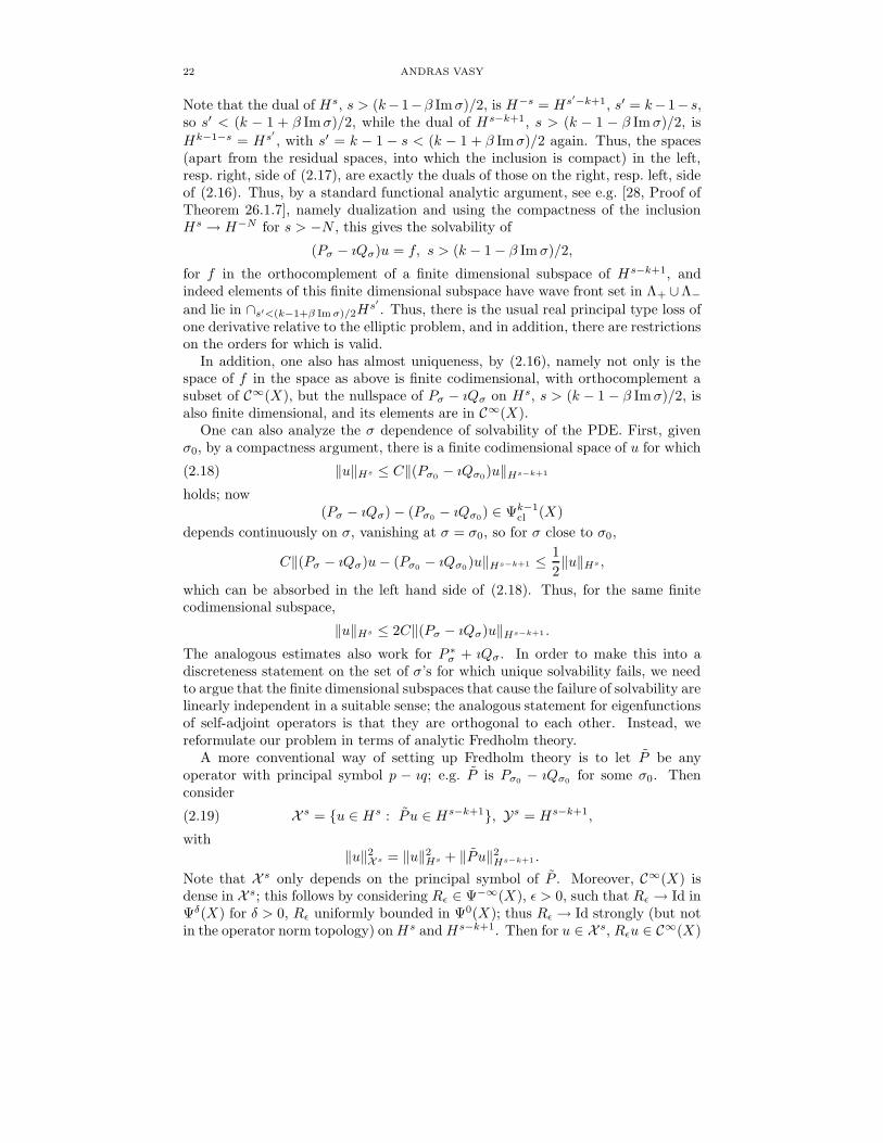
We make the following non-trapping assumption. For α ∈ S∗X , let γ+(α), resp.γ−(α) denote the image of the forward, resp. backward, half-bicharacteristic fromα. We write γ±(α) → L± (and say γ±(α) tends to L±) if given any neighborhoodO of L±, γ±(α) ∩ O 6= ∅; by the source/sink property this implies that the points
10Thus, they are connected components in the extended sense that they may be empty.11An extreme example would be Λ± = Σ±. Another extreme is if one or both are empty.12If Hp is radial at L±, this is independent of the choice of the density ν. Indeed, with respect
to fν, the adjoint of Pσ is f−1P ∗σf , with P ∗
σ denoting the adjoint with respect to ν. This is
P ∗σ + f−1[P ∗
σ , f ], and the principal symbol of f−1[P ∗σ , f ] ∈ Ψk−1
cl (X) vanishes at L± as Hpf = 0.In general, we can only change the density by factors f with Hpf |L±
= 0, which in Kerr-de Sitter
space-times would mean factors independent of φ at the event horizon. A similar argument showsthe independence of the condition from the choice of f when one replaces Pσ by fPσ , under thesame conditions: either radiality, or just Hpf |L±
= 0.
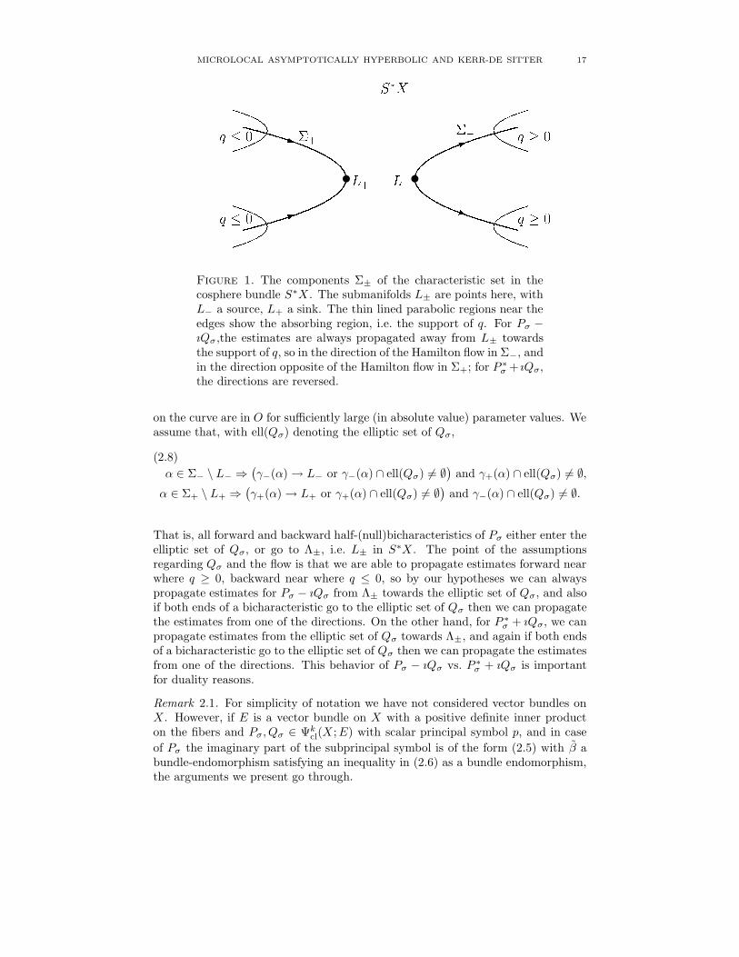
MICROLOCAL ASYMPTOTICALLY HYPERBOLIC AND KERR-DE SITTER 17
Figure 1. The components Σ± of the characteristic set in thecosphere bundle S∗X . The submanifolds L± are points here, withL− a source, L+ a sink. The thin lined parabolic regions near theedges show the absorbing region, i.e. the support of q. For Pσ −ıQσ ,the estimates are always propagated away from L± towardsthe support of q, so in the direction of the Hamilton flow in Σ−, andin the direction opposite of the Hamilton flow in Σ+; for P ∗
σ + ıQσ,the directions are reversed.
on the curve are in O for sufficiently large (in absolute value) parameter values. Weassume that, with ell(Qσ) denoting the elliptic set of Qσ,
(2.8)
α ∈ Σ− \ L− ⇒(γ−(α) → L− or γ−(α) ∩ ell(Qσ) 6= ∅
)and γ+(α) ∩ ell(Qσ) 6= ∅,
α ∈ Σ+ \ L+ ⇒(γ+(α) → L+ or γ+(α) ∩ ell(Qσ) 6= ∅
)and γ−(α) ∩ ell(Qσ) 6= ∅.
That is, all forward and backward half-(null)bicharacteristics of Pσ either enter theelliptic set of Qσ, or go to Λ±, i.e. L± in S∗X . The point of the assumptionsregarding Qσ and the flow is that we are able to propagate estimates forward nearwhere q ≥ 0, backward near where q ≤ 0, so by our hypotheses we can alwayspropagate estimates for Pσ − ıQσ from Λ± towards the elliptic set of Qσ , and alsoif both ends of a bicharacteristic go to the elliptic set of Qσ then we can propagatethe estimates from one of the directions. On the other hand, for P ∗
σ + ıQσ, we canpropagate estimates from the elliptic set of Qσ towards Λ±, and again if both endsof a bicharacteristic go to the elliptic set of Qσ then we can propagate the estimatesfrom one of the directions. This behavior of Pσ − ıQσ vs. P ∗
σ + ıQσ is importantfor duality reasons.
Remark 2.1. For simplicity of notation we have not considered vector bundles onX . However, if E is a vector bundle on X with a positive definite inner producton the fibers and Pσ , Qσ ∈ Ψk
cl(X ; E) with scalar principal symbol p, and in case
of Pσ the imaginary part of the subprincipal symbol is of the form (2.5) with β abundle-endomorphism satisfying an inequality in (2.6) as a bundle endomorphism,the arguments we present go through.
18 ANDRAS VASY
2.3. Elliptic and microhyperbolic points. We now turn to analysis. First, bythe usual elliptic theory, on the elliptic set of Pσ − ıQσ, so both on the elliptic setof Pσ and on the elliptic set of Qσ, one has elliptic estimates13: for all s and N ,and for all B, G ∈ Ψ0(X) with G elliptic on WF′(B),
(2.9) ‖Bu‖Hs ≤ C(‖G(Pσ − ıQσ)u‖Hs−k + ‖u‖H−N ),
with the estimate also holding for P ∗σ + ıQσ. By propagation of singularities, in
Σ\ (WF′(Qσ)∪L+ ∪L−), one can propagate regularity estimates either forward orbackward along bicharacteristics, i.e. for all s and N , and for all A, B, G ∈ Ψ0(X)such that WF′(G) ∩ WF′(Qσ) = ∅, and forward (or backward) bicharacteristicsfrom WF′(B) reach the elliptic set of A, while remaining in the elliptic set of G,one has estimates
(2.10) ‖Bu‖Hs ≤ C(‖GPσu‖Hs−k+1 + ‖Au‖Hs + ‖u‖H−N ).
Here Pσ can be replaced by Pσ − ıQσ or P ∗σ + ıQσ by the condition on WF′(G);
namely GQσ ∈ Ψ−∞(X), and can thus be absorbed into the ‖u‖H−N term. Asusual, there is a loss of one derivative compared to the elliptic estimate, i.e. theassumption on Pσu is Hs−k+1, not Hs−k, and one needs to make Hs assumptionson Au, i.e. regularity propagates.
2.4. Analysis near Λ±. At Λ±, for s ≥ m > (k − 1 − β Im σ)/2, β given by thesubprincipal symbol at Λ±, we can propagate estimates away from Λ±:
Proposition 2.2. For Im σ ≥ 0, let14 β = βinf, for Im σ < 0, let β = βsup. For allN , for s ≥ m > (k−1−β Im σ)/2, and for all A, B, G ∈ Ψ0(X) such that WF′(G)∩WF′(Qσ) = ∅, A elliptic at Λ±, and forward (or backward) bicharacteristics fromWF′(B) tend to Λ±, with closure in the elliptic set of G, one has estimates
(2.11) ‖Bu‖Hs ≤ C(‖GPσu‖Hs−k+1 + ‖Au‖Hm + ‖u‖H−N ),
in the sense that if u ∈ H−N , Au ∈ Hm and GPσu ∈ Hs−k+1, then Bu ∈ Hs, and(2.11) holds. In fact, Au can be dropped from the right hand side (but one mustassume Au ∈ Hm):
(2.12) Au ∈ Hm ⇒ ‖Bu‖Hs ≤ C(‖GPσu‖Hs−k+1 + ‖u‖H−N ),
where u ∈ H−N and GPσu ∈ Hs−k+1 is considered implied by the right hand side.Note that Au does not appear on the right hand side, hence the display before theestimate.
This is completely analogous to Melrose’s estimates in asymptotically Euclideanscattering theory at the radial sets [35, Section 9]. Note that the Hs regularityof Bu is ‘free’ in the sense that we do not need to impose Hs assumptions on uanywhere; merely Hm at Λ± does the job; of course, on Pσu one must make theHs−k+1 assumption, i.e. the loss of one derivative compared to the elliptic setting.At the cost of changing regularity, one can propagate estimate towards Λ±. Keepingin mind that for P ∗
σ the subprincipal symbol becomes βσ, we have the following:
13Our convention in estimates such as (2.9) and (2.10) is that if one assumes that all thequantities on the right hand side are in the function spaces indicated by the norms then so is thequantity on the left hand side, and the estimate holds. As we see below, at Λ± not all relevantfunction space statements appear in the estimate, so we need to be more explicit there.
14Note that this is consistent with (2.7).
MICROLOCAL ASYMPTOTICALLY HYPERBOLIC AND KERR-DE SITTER 19
Proposition 2.3. For Im σ > 0, let15 β = βsup, for Im σ ≤ 0, let β = βinf . Fors < (k− 1−β Im σ)/2, for all N , and for all A, B, G ∈ Ψ0(X) such that WF′(G)∩WF′(Qσ) = ∅, B, G elliptic at Λ±, and forward (or backward) bicharacteristicsfrom WF′(B) \Λ± reach WF′(A), while remaining in the elliptic set of G, one hasestimates
(2.13) ‖Bu‖Hs ≤ C(‖GP ∗σ u‖Hs−k+1 + ‖Au‖Hs + ‖u‖H−N ).
Proof of Propositions 2.2-2.3. It suffices to prove that there exist Oj open withL± ⊂ Oj+1 ⊂ Oj , ∩∞
j=1Oj = L±, and Aj , Bj , Gj with WF′ in Oj , Bj elliptic on L±,such that the statements of the propositions hold. Indeed, in case of Proposition 2.2the general case follows by taking j such that A, G are elliptic on Oj , use theestimate for Aj , Bj , Gj , where the right hand side then can be estimated by A andG, and then use microlocal ellipticity, propagation of singularities and a coveringargument to prove the proposition. In case of Proposition 2.3, the general casefollows by taking j such that G, B are elliptic on Oj , so all forward (or backward)bicharacteristics from Oj\Λ± reach WF′(A), thus microlocal ellipticity, propagationof singularities and a covering argument proves ‖Aju‖Hs ≤ C(‖GP ∗
σ u‖Hs−k+1 +‖Au‖Hs +‖u‖H−N ), and then the special case of the proposition for this Oj gives anestimate for ‖Bju‖Hs in terms of the same quantities. The full estimate for ‖Bu‖Hs
is then again a straightforward consequence of microlocal ellipticity, propagation ofsingularities and a covering argument.
We now consider commutants C∗ε Cε with Cε ∈ Ψs−(k−1)/2−δ(X) for ε > 0,
uniformly bounded in Ψs−(k−1)/2(X) as ε → 0; with the ε-dependence used toregularize the argument. More precisely, let
c = φ(ρ0)ρ−s+(k−1)/2, cε = c(1 + ερ−1)−δ,
where φ ∈ C∞c (R) is identically 1 near 0, φ′ ≤ 0 and φ is supported sufficiently close
to 0 so that
(2.14) ρ0 ∈ supp dφ ⇒ ∓ρk−10 Hpρ0 > 0;
such φ exists by (2.4). Note that the sign of Hpρ−s+(k−1)/2 depends on the sign of
−s+(k−1)/2 which explains the difference between s > (k−1)/2 and s < (k−1)/2in Propositions 2.2-2.3 when there are no other contributions to the threshold valueof s. The contribution of the subprincipal symbol, however, shifts the critical value(k − 1)/2.
Now let C ∈ Ψs−(k−1)/2(X) have principal symbol c, and have WF′(C) ⊂supp φ ρ0, and let Cε = CSε, Sε ∈ Ψ−δ(X) uniformly bounded in Ψ0(X) for
ε > 0, converging to Id in Ψδ′
(X) for δ′ > 0 as ε → 0, with principal symbol(1 + ερ−1)−δ. Thus, the principal symbol of Cε is cε.
First, consider (2.11). Then
σ2s(ı(P∗σ C∗
ε Cε − C∗ε CεPσ)) = σ1(P
∗σ − Pσ)c2
ε + 2cεHpcε
= ∓2
(−β Im σβ0φ + β0
(−s +
k − 1
2
)φ ∓ (ρk−1
Hpρ0)φ′ + δβ0
ε
ρ + εφ
)
φρ−2s(1 + ερ−1)−δ ,
15Note the switch compared to Proposition 2.2! Also, β does not matter when Im σ = 0; wedefine it here so that the two Propositions are consistent via dualization, which reverses the signof the imaginary part.
20 ANDRAS VASY
so
∓σ2s(ı(P∗σ C∗
ε Cε − C∗ε CεPσ))
≤ −2β0
(s − k − 1
2+ β Im σ − δ
)ρ−2s(1 + ερ−1)−δφ2
+ 2(∓ρk−1Hpρ0)ρ
−2s(1 + ερ−1)−δφ′φ.
(2.15)
Here the first term on the right hand side is negative if s−(k−1)/2+β Im σ−δ > 0
(since β Im σ ≥ β Im σ by our definition of β), and this is the same sign as thatof φ′ term; the presence of δ (needed for the regularization) is the reason for theappearance of m in the estimate. To avoid using the sharp Garding inequality, wechoose φ so that
√−φφ′ is C∞, and then
ı(P ∗σ C∗
ε Cε − C∗ε CεPσ) = −S∗
ε (B∗B + B∗1B1 + B∗
2,εB2,ε)Sε + Fε,
with B, B1, B2,ε ∈ Ψs(X), B2,ε uniformly bounded in Ψs(X) as ε → 0, Fε uniformlybounded in Ψ2s−1(X), and σs(B) an elliptic multiple of φ(ρ0)ρ
−s. Computing
〈ı(P ∗σ C∗
ε Cε − C∗ε CεPσ)u, u〉 = 〈ıC∗
ε Cεu, Pσu〉 − 〈ıPσ , C∗ε Cεu〉,
using Cauchy-Schwartz on the right hand side, a standard functional analytic ar-gument (see, for instance, Melrose [35, Proof of Proposition 7 and Section 9]) givesan estimate for Bu, showing u is in Hs on the elliptic set of B, provided u is mi-crolocally in Hs−δ. A standard inductive argument, starting with s − δ = m andimproving regularity by ≤ 1/2 in each step proves (2.11).
For (2.13), the argument is similar, but we want to change the sign of the firstterm on the right hand side of (2.15), i.e. we want it to be positive. This is satisfied
if s − (k − 1)/2 + β Im σ − δ < 0 (since β Im σ ≤ β Im σ by our definition of β inProposition 2.3), hence (as δ > 0) if s− (k − 1)/2 + β Im σ < 0, so regularization isnot an issue. On the other hand, φ′ now has the wrong sign, so one needs to makean assumption on supp dφ, which is the Au term in (2.13). Since the details arestandard, see [35, Section 9], we leave these to the reader.
Remark 2.4. Fixing a φ, it follows from the proof that the same φ works for (small)smooth perturbations of Pσ , even if those perturbations do not preserve the eventhorizon, namely even if (2.4) does not hold any more: only its implication, (2.14),on supp dφ matters, which is stable under perturbations. Moreover, as the rescaledHamilton vector field ρk−1
Hp is a smooth vector field tangent to the boundary ofthe fiber-compactified cotangent bundle, i.e. a b-vector field, and as such dependssmoothly on the principal symbol, and it is non-degenerate radially by (2.3), theweight, which provides the positivity at the radial points in the proof above, stillgives a positive Hamilton derivative for small perturbations. Since this propositionthus holds for C∞ perturbations of Pσ (indeed, even pseudodifferential ones), andthis proposition is the only delicate estimate we use, and it is only marginally so,we deduce that all the other results below also hold in this generality.
2.5. Complex absorption. Finally, one has propagation estimates for complexabsorbing operators, requiring a sign condition. (See for instance [40] and [13] inthe semiclassical setting; the changes are minor in the ‘classical’ setting.) First,one can propagate regularity to WF′(Qσ) (of course, in the elliptic set of Qσ onehas a priori regularity). Namely, for all s and N , and for all A, B, G ∈ Ψ0(X) suchthat q ≤ 0, resp. q ≥ 0, on WF′(G), and forward, resp. backward, bicharacteristics
MICROLOCAL ASYMPTOTICALLY HYPERBOLIC AND KERR-DE SITTER 21
of Pσ from WF′(B) reach the elliptic set of A, while remaining in the elliptic set ofG, one has the usual propagation estimates
‖Bu‖Hs ≤ C(‖G(Pσ − ıQσ)u‖Hs−k+1 + ‖Au‖Hs + ‖u‖H−N ).
Thus, for q ≥ 0 one can propagate regularity in the forward direction along theHamilton flow, while for q ≤ 0 one can do so in the backward direction.
On the other hand, one can propagate regularity away from the elliptic set of Qσ.Namely, for all s and N , and for all B, G ∈ Ψ0(X) such that q ≤ 0, resp. q ≥ 0, onWF′(G), and forward, resp. backward, bicharacteristics of Pσ from WF′(B) reachthe elliptic set of Qσ, while remaining in the elliptic set of G, one has the usualpropagation estimates
‖Bu‖Hs ≤ C(‖G(Pσ − ıQσ)u‖Hs−k+1 + ‖u‖H−N ).
Again, for q ≥ 0 one can propagate regularity in the forward direction along theHamilton flow, while for q ≤ 0 one can do so in the backward direction. At thecost of reversing the signs of q, this also gives that for all s and N , and for allB, G ∈ Ψ0(X) such that q ≥ 0, resp. q ≤ 0, on WF′(G), and forward, resp.backward, bicharacteristics of Pσ from WF′(B) reach the elliptic set of Qσ, whileremaining in the elliptic set of G, one has the usual propagation estimates
‖Bu‖Hs ≤ C(‖G(P ∗σ + ıQσ)u‖Hs−k+1 + ‖u‖H−N ).
Remark 2.5. As mentioned in the introduction, these complex absorption methodscould be replaced in specific cases, including all the specific examples we discusshere, by adding a boundary Y instead, provided that the Hamilton flow is well-behaved relative to the base space, namely inside the characteristic set Hp is nottangent to T ∗
YX with orbits crossing T ∗
YX in the opposite directions in Σ± in the
following way. If Y is defined by y which is positive on ‘our side’ U with U asdiscussed at the beginning of Subsection 2.2, we need ±Hpy|Y > 0 on Σ±. Thenthe functional analysis described in [28, Proof of Theorem 23.2.2], see also [47,Proof of Lemma 4.14], can be used to prove analogues of the results we give below
on X+ = y ≥ 0. For instance, if one has a Lorentzian metric on X near Y ,
and Y is space-like, then (up to the sign) this statement holds with Σ± being thetwo components of the characteristic set. However, in the author’s opinion, thisdetracts from the clarity of the microlocal analysis by introducing projection tophysical space in an essential way.
2.6. Global estimates. Piecing together these estimates, using non-trapping topropagate estimates from Λ± (as well as from one end of a bicharacteristic whichintersects the elliptic set of q in both directions) one has that for any N , and forany s ≥ m > (k − 1 − β Im σ)/2, and for any A ∈ Ψ0(X) elliptic at Λ+ ∪ Λ−,
‖u‖Hs ≤ C(‖(Pσ − ıQσ)u‖Hs−k+1 + ‖Au‖Hm + ‖u‖H−N ),
provided q ≥ 0 on the (forward) flow-out of Λ−, and q ≤ 0 on the (backward)flowout of Λ+. This implies that for any s ≥ m > (k − 1 − β Im σ)/2,
(2.16) ‖u‖Hs ≤ C(‖(Pσ − ıQσ)u‖Hs−k+1 + ‖u‖Hm).
On the other hand, for any N and for any s < (k−1+β Im σ)/2 (recalling that theadjoint switches the sign of the imaginary part of the subprincipal symbol), andunder the same conditions on q,
(2.17) ‖u‖Hs ≤ C(‖(P ∗σ + ıQσ)u‖Hs−k+1 + ‖u‖H−N ).
22 ANDRAS VASY
Note that the dual of Hs, s > (k−1−β Im σ)/2, is H−s = Hs′−k+1, s′ = k−1− s,so s′ < (k − 1 + β Im σ)/2, while the dual of Hs−k+1, s > (k − 1 − β Im σ)/2, is
Hk−1−s = Hs′
, with s′ = k − 1 − s < (k − 1 + β Im σ)/2 again. Thus, the spaces(apart from the residual spaces, into which the inclusion is compact) in the left,resp. right, side of (2.17), are exactly the duals of those on the right, resp. left, sideof (2.16). Thus, by a standard functional analytic argument, see e.g. [28, Proof ofTheorem 26.1.7], namely dualization and using the compactness of the inclusionHs → H−N for s > −N , this gives the solvability of
(Pσ − ıQσ)u = f, s > (k − 1 − β Im σ)/2,
for f in the orthocomplement of a finite dimensional subspace of Hs−k+1, andindeed elements of this finite dimensional subspace have wave front set in Λ+ ∪Λ−
and lie in ∩s′<(k−1+β Im σ)/2Hs′
. Thus, there is the usual real principal type loss ofone derivative relative to the elliptic problem, and in addition, there are restrictionson the orders for which is valid.
In addition, one also has almost uniqueness, by (2.16), namely not only is thespace of f in the space as above is finite codimensional, with orthocomplement asubset of C∞(X), but the nullspace of Pσ − ıQσ on Hs, s > (k − 1 − β Im σ)/2, isalso finite dimensional, and its elements are in C∞(X).
One can also analyze the σ dependence of solvability of the PDE. First, givenσ0, by a compactness argument, there is a finite codimensional space of u for which
(2.18) ‖u‖Hs ≤ C‖(Pσ0− ıQσ0
)u‖Hs−k+1
holds; now(Pσ − ıQσ) − (Pσ0
− ıQσ0) ∈ Ψk−1
cl (X)
depends continuously on σ, vanishing at σ = σ0, so for σ close to σ0,
C‖(Pσ − ıQσ)u − (Pσ0− ıQσ0
)u‖Hs−k+1 ≤ 1
2‖u‖Hs ,
which can be absorbed in the left hand side of (2.18). Thus, for the same finitecodimensional subspace,
‖u‖Hs ≤ 2C‖(Pσ − ıQσ)u‖Hs−k+1 .
The analogous estimates also work for P ∗σ + ıQσ. In order to make this into a
discreteness statement on the set of σ’s for which unique solvability fails, we needto argue that the finite dimensional subspaces that cause the failure of solvability arelinearly independent in a suitable sense; the analogous statement for eigenfunctionsof self-adjoint operators is that they are orthogonal to each other. Instead, wereformulate our problem in terms of analytic Fredholm theory.
A more conventional way of setting up Fredholm theory is to let P be anyoperator with principal symbol p − ıq; e.g. P is Pσ0
− ıQσ0for some σ0. Then
consider
(2.19) X s = u ∈ Hs : P u ∈ Hs−k+1, Ys = Hs−k+1,
with‖u‖2
X s = ‖u‖2Hs + ‖Pu‖2
Hs−k+1 .
Note that X s only depends on the principal symbol of P . Moreover, C∞(X) isdense in X s; this follows by considering Rε ∈ Ψ−∞(X), ε > 0, such that Rε → Id inΨδ(X) for δ > 0, Rε uniformly bounded in Ψ0(X); thus Rε → Id strongly (but notin the operator norm topology) on Hs and Hs−k+1. Then for u ∈ X s, Rεu ∈ C∞(X)
MICROLOCAL ASYMPTOTICALLY HYPERBOLIC AND KERR-DE SITTER 23
for ε > 0, Rεu → u in Hs and PRεu = RεP u + [P , Rε]u, so the first term on the
right converges to P u in Hs−k+1, while [P , Rε] is uniformly bounded in Ψk−1(X),converging to 0 in Ψk−1+δ(X) for δ > 0, so converging to 0 strongly as a map
Hs → Hs−k+1. Thus, [P , Rε]u → 0 in Hs−k+1, and we conclude that Rεu → u inX s. (In fact, X s is a first-order coisotropic space, more general function space ofthis nature are discussed by Melrose, Vasy and Wunsch in [38, Appendix A].)
With these preliminaries,
Pσ − ıQσ : X s → Ys
is Fredholm for each σ with s ≥ m > (k − 1 − β Im σ)/2, and is an analytic familyof bounded operators in this half-plane of σ’s.
Theorem 2.6. Let Pσ, Qσ be as above, and X s, Ys as in (2.19). If k−1−2s > 0,let β = βinf , if k − 1 − 2s < 0, let β = βsup. Then
Pσ − ıQσ : X s → Ys
is an analytic family of Fredholm operators on
(2.20) Cs = σ ∈ C : Im σ > β−1(k − 1 − 2s).Thus, analytic Fredholm theory applies, giving meromorphy of the inverse pro-
vided the inverse exists for a particular value of σ.
Remark 2.7. Note that the Fredholm property means that P ∗σ +ıQσ is also Fredholm
on the dual spaces; this can also be seen directly from the estimates. The analogueof this remark also applies to the semiclassical discussion below.
2.7. Semiclassical estimates. For this reason, and also for wave propagation, wealso want to know the |σ| → ∞ asymptotics of Pσ−ıσ and P ∗
σ +ıQσ; here Pσ , Qσ areoperators with a large parameter. As discussed earlier, this can be translated intoa semiclassical problem, i.e. one obtains families of operators Ph,z, with h = |σ|−1,and z corresponding to σ/|σ| in the unit circle in C. As usual, we multiply throughby hk for convenient notation when we define Ph,z:
Ph,z = hkPh−1z ∈ Ψk~,cl(X).
From now on, we merely require Ph,z, Qh,z ∈ Ψk~,cl(X). Then the semiclassical
principal symbol p~,z, z ∈ O ⊂ C, 0 /∈ O compact, which is a function on T ∗X , haslimit p at infinity in the fibers of the cotangent bundle, so is in particular real inthe limit. More precisely, as in the classical setting, but now ρ made smooth at thezero section as well (so is not homogeneous there), we consider
ρkp~,z ∈ C∞(T∗X × O);
then ρkp~,z|S∗X×O = ρkp, where S∗X = ∂T∗X . We assume that p~,z is real
when z is real. We shall be interested in Im z ≥ −Ch, which corresponds toIm σ ≥ −C (recall that Im σ 0 is where we expect holomorphy). Note that whenIm z = O(h), Im p~,z still vanishes, as the contribution of Im z is semiclassicallysubprincipal in view of the order h vanishing.
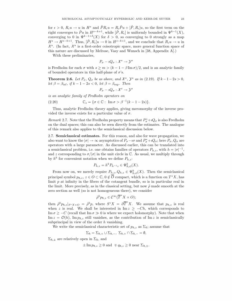
We write the semiclassical characteristic set of p~,z as Σ~; assume that
Σ~ = Σ~,+ ∪ Σ~,−, Σ~,+ ∩ Σ~,− = ∅,Σ~,± are relatively open in Σ~, and
± Im p~,z ≥ 0 and ∓ q~,z ≥ 0 near Σ~,±.
24 ANDRAS VASY
Figure 2. The components Σ~,± of the semiclassical characteris-
tic set in T∗X , which are now two-dimensional in the figure. The
cosphere bundle is the horizontal plane at the bottom of the pic-ture; the intersection of this figure with the cosphere bundle iswhat is shown on Figure 1. The submanifolds L± are still points,with L− a source, L+ a sink. The red lines are bicharacteristics,
with the thick ones inside S∗X = ∂T∗X . The blue regions near
the edges show the absorbing region, i.e. the support of q. ForPh,z − ıQh,z, the estimates are always propagated away from L±
towards the support of q, so in the direction of the Hamilton flowin Σ~,−, and in the direction opposite of the Hamilton flow in Σ~,+;for P ∗
h,z + ıQh,z, the directions are reversed.
Microlocal results analogous to the classical results also exist in the semiclassical
setting. In the interior of T∗X , i.e. in T ∗X , only the microlocal elliptic, microhyper-
bolic and complex absorption estimates are relevant. At L± ⊂ S∗X we in additionneed the analogue of Propositions 2.2-2.3. As these are the only non-standard es-timates, though they are very similar to estimates of [49], where, however, onlyglobal estimates were stated, we explicitly state these here and indicate the veryminor changes needed in the proof compared to Propositions 2.2-2.3.
Proposition 2.8. For all N , for s ≥ m > (k − 1 − β Im σ)/2, σ = h−1z, and forall A, B, G ∈ Ψ0
~(X) such that WF′
h(G) ∩ WF′h(Qσ) = ∅, A elliptic at L±, and
forward (or backward) bicharacteristics from WF′h(B) tend to L±, with closure in
the elliptic set of G, one has estimates
(2.21) Au ∈ Hmh ⇒ ‖Bu‖Hs
h≤ C(h−1‖GPh,zu‖Hs−k+1
h
+ h‖u‖H−Nh
),
where, as usual, GPh,zu ∈ Hs−k+1h and u ∈ H−N
h are assumptions implied by theright hand side.
Proposition 2.9. For s < (k − 1 − β Im σ)/2, for all N , σ = h−1z, and for allA, B, G ∈ Ψ0
~(X) such that WF′
h(G) ∩ WF′h(Qσ) = ∅, B, G elliptic at L±, and
MICROLOCAL ASYMPTOTICALLY HYPERBOLIC AND KERR-DE SITTER 25
forward (or backward) bicharacteristics from WF′h(B) \ L± reach WF′
h(A), whileremaining in the elliptic set of G, one has estimates
(2.22) ‖Bu‖Hsh≤ C(h−1‖GP ∗
h,zu‖Hs−k+1
h
+ ‖Au‖Hsh
+ h‖u‖H−Nh
).
Proof. We just need to localize in ρ in addition to ρ0; such a localization in theclassical setting is implied by working on S∗X or with homogeneous symbols. Weachieve this by modifying the localizer φ in the commutant constructed in the proofof Propositions 2.2-2.3. As already remarked, the proof is much like at radial pointsin semiclassical scattering on asymptotically Euclidean spaces, studied by Vasy andZworski [49], but we need to be more careful about localization in ρ0 and ρ as weare assuming less about the structure.
First, note that L± is defined by ρ = 0, ρ0 = 0, so ρ2 +ρ0 is a quadratic definingfunction of L±. Thus, let φ ∈ C∞
c (R) be identically 1 near 0, φ′ ≤ 0 and φ supportedsufficiently close to 0 so that
ρ2 + ρ0 ∈ supp dφ ⇒ ∓ρk−1(Hpρ0 + 2ρHpρ) > 0
and
ρ2 + ρ0 ∈ suppφ ⇒ ∓ρk−2Hpρ > 0.
Such φ exists by (2.3) and (2.4) as
∓ρ(Hpρ0 + 2ρHpρ) ≥ β1ρ0 + 2β0ρ2 −O((ρ2 + ρ0)
3/2).
Then let c be given by
c = φ(ρ0 + ρ2)ρ−s+(k−1)/2, cε = c(1 + ερ−1)−δ.
The rest of the proof proceeds exactly as for Propositions 2.2-2.3.
We first show that under extra assumptions, giving semiclassical ellipticity forIm z bounded away from 0, we have non-trapping estimates. So assume that for| Im z| > ε > 0, p~,z is semiclassically elliptic on T ∗X (but not necessarily at S∗X =
∂T∗X , where the standard principal symbol p already describes the behavior). Also
assume that ± Im p~,z ≥ 0 near the classical characteristic set Σ~,± ⊂ S∗X . Thenthe semiclassical version of the classical results (with ellipticity in T ∗X makingthese trivial except at S∗X) apply. Let Hs
h denote the usual semiclassical functionspaces. Then, on the one hand, for any s ≥ m > (k − 1 − β Im z/h)/2, h < h0,
(2.23) ‖u‖Hsh≤ Ch−1(‖(Ph,z − ıQh,z)u‖Hs−k+1
h+ h2‖u‖Hm
h),
and on the other hand, for any N and for any s < (k − 1 + β Im z/h)/2, h < h0,
(2.24) ‖u‖Hsh≤ Ch−1(‖(P ∗
h,z + ıQh,z)u‖Hs−k+1
h
+ h2‖u‖H−Nh
).
The h2 term can be absorbed in the left hand side for sufficiently small h, so weautomatically obtain invertibility of Ph,z − ıQh,z.
In particular, Ph,z − ıQh,z is invertible for z = ı and h small, i.e. Pσ − ıQσ is suchfor σ pure imaginary with large positive imaginary part, proving the meromorphyof Pσ − ıQσ under these extra assumptions. Note also that for instance
‖u‖2H1
|σ|−1= ‖u‖2
L2 + |σ|−2‖du‖2L2 , ‖u‖H0
|σ|−1= ‖u‖L2 ,
(with the norms with respect to any positive definite inner product).
26 ANDRAS VASY
Theorem 2.10. Let Pσ, Qσ, β, Cs be as above, and X s, Ys as in (2.19). Then,for σ ∈ Cs,
Pσ − ıQσ : X s → Ys
has a meromorphic inverse
R(σ) : Ys → X s.
Moreover, for all ε > 0 there is C > 0 such that it is invertible in Im σ > C+ε|Reσ|,and non-trapping estimates hold:
‖R(σ)f‖Hs
|σ|−1≤ C ′|σ|−k+1‖f‖Hs−1
|σ|−1.
To deal with estimates for z (almost) real, we need additional assumptions. Wemake the non-trapping assumption into a definition:
Definition 2.11. We say that p~,z − ıq~,z is semiclassically non-trapping if thebicharacteristics from any point in Σ~ \ (L+ ∪L−) flow to ell(q~,z)∪L+ (i.e. eitherenter ell(q~,z) at some finite time, or tend to L+) in the forward direction, and toell(q~,z) ∪ L− in the backward direction.
Remark 2.12. The part of the semiclassically non-trapping property on S∗X isjust the classical non-trapping property; thus, the point is its extension into to the
interior T ∗X of T∗X . Since the classical principal symbol is assumed real, there
did not need to be any additional restrictions on Im p~,z there.
The semiclassical version of all of the above estimates are then applicable forIm z ≥ −Ch, and one obtains on the one hand that for any s ≥ m > (k − 1 −β Im z/h)/2, h < h0,
(2.25) ‖u‖Hsh≤ Ch−1(‖(Ph,z − ıQh,z)u‖Hs−k+1
h+ h2‖u‖Hm
h),
On the other hand, for any N and for any s < (k − 1 + β Im z/h)/2, h < h0,
(2.26) ‖u‖Hsh≤ Ch−1(‖(P ∗
h,z + ıQh,z)u‖Hs−k+1
h
+ h2‖u‖H−Nh
),
The h2 term can again be absorbed in the left hand side for sufficiently small h, sowe automatically obtain invertibility of Ph,z − ıQh,z.
Translated into the classical setting this gives
Theorem 2.13. Let Pσ, Qσ, Cs, β be as above, in particular semiclassically non-trapping, and X s, Ys as in (2.19). Let C > 0. Then there exists σ0 such that
R(σ) : Ys → X s,
is holomorphic in σ : Im σ > −C, |Re σ| > σ0, assumed to be a subset of Cs,and non-trapping estimates
‖R(σ)f‖Hs
|σ|−1≤ C ′|σ|−k+1‖f‖Hs−k+1
|σ|−1
hold. For s = 1, k = 2 this states that for |Reσ| > σ0, Im σ > −C,
‖R(σ)f‖2L2 + |σ|−2‖dR(σ)‖2
L2 ≤ C ′′|σ|−2‖f‖2L2 .
Analogous results work for other Sobolev spaces; H1h was chosen above for sim-
plicity.
MICROLOCAL ASYMPTOTICALLY HYPERBOLIC AND KERR-DE SITTER 27
Remark 2.14. We emphasize that if semiclassical non-trapping assumptions aremade, but not ellipticity for z non-real, meromorphy still follows by taking h smalland z > 0, say, to get a point of invertibility. This is useful because one caneliminate the need to conjugate by a factor to induce such ellipticity when theresulting estimate is irrelevant. (Mostly estimates in strips for h−1z, i.e. O(h)estimates for z, matter.) However, there is a cost: while only finitely many polescan lie in any strip | Im σ| < C, there is no need for this statement to hold if weallow Im σ > −C. Since, for the application to the wave equation, Im σ dependson the a priori growth rate of the solution u which we are Mellin transforming, thiswould mean that depending on the a priori growth rate one could get more (fastergrowing) terms in the expansion of u if one relaxes the growth condition on u.
While we stated just the global results here, of course one has microlocal esti-mates for the solution. In particular we have the following, stated in the semiclas-sical language, as immediate from the estimates used to derive from the Fredholmproperty:
Theorem 2.15. Let Pσ, Qσ, β be as above, in particular semiclassically non-trapping, and X s, Ys as in (2.19).
For Re z > 0 and s′ > s, the resolvent Rh,z is semiclassically outgoing with a loss
of h−1 in the sense that if α ∈ T∗X∩Σ~,±, and if for the forward (+), resp. backward
(−), bicharacteristic γ±, from α, WFs′−k+1h (f) ∩ γ± = ∅ then α /∈ WFs′
h (hRh,zf).
In fact, for any s′ ∈ R, the resolvent Rh,z extends to f ∈ Hs′
h (X), with non-trapping bounds, provided that WFs
h(f) ∩ (L+ ∪ L−) = ∅. The semiclassicallyoutgoing with a loss of h−1 result holds for such f and s′ as well.
Proof. The only part that is not immediate by what has been discussed is the lastclaim. This follows immediately, however, by microlocal solvability in arbitraryordered Sobolev spaces away from the radial points (i.e. solvability modulo C∞,with semiclassical estimates), combined with our preceding results to deal with thissmooth remainder plus the contribution near L+ ∪L−, which are assumed to be inHs
h(X).
This result is needed for gluing constructions as in [13], namely polynomiallybounded trapping with appropriate microlocal geometry can be glued to our re-solvent. Furthermore, it gives non-trapping estimates microlocally away from thetrapped set provided the overall (trapped) resolvent is polynomially bounded asshown by Datchev and Vasy [14].
Definition 2.16. Suppose K± ⊂ T ∗X is compact, and O± is a neighborhood ofK with compact closure and O± ∩ Σ~ ⊂ Σ~,±. We say that p~,z is semiclassicallylocally mildly trapping of order κ in a C0-strip if
(i) there is a function16 F ∈ C∞(T ∗X), F ≥ 2 on K±, F ≤ 1 on T ∗X \ O±,and for α ∈ (O± \ K±) ∩ Σ~,±, (Hp~,z
F )(α) = 0 implies (H2p~,z
F )(α) < 0;and
16 For ε > 0, such a function F provides an escape function, F = e−CF Hp~,z F on the set
where 1 + ε ≤ F ≤ 2 − ε. Namely, by taking C > 0 sufficiently large, Hp~,z F < 0 there; thus,
every bicharacteristic must leave the compact set F−1([1 + ε, 2 − ε]) in finite time. However, theexistence of such an F is a stronger statement than that of an escape function: a bicharacteristicsegment cannot leave F−1([1 + ε, 2 − ε]) via the boundary F = 2 − ε in both directions since F
cannot have a local minimum. This is exactly the way this condition is used in [13].
28 ANDRAS VASY
(ii) there exists Qh,z ∈ Ψ~(X) with WF′h(Qh,z)∩K± = ∅, ∓q~,z ≥ 0 near Σ~,±,
q~,z elliptic on Σ~ \ (O+ ∪ O−) and h0 > 0 such that if Im z > −C0h andh < h0 then
(2.27) ‖(Ph,z − ıQh,z)−1f‖Hs
h≤ Ch−κ−1‖f‖Hs−k+1
h
, f ∈ Hs−k+1h .
We say that p~,z − ıq~,z is semiclassically mildly trapping of order κ in a C0-strip if it is semiclassically locally mildly trapping of order κ in a C0-strip and if thebicharacteristics from any point in Σ~,+ \ (L+ ∪K+) flow to q~,z < 0∪O+ in thebackward direction and to q~,z < 0∪O+ ∪L+ in the forward direction, while thebicharacteristics from any point in Σ~,− \ (L− ∪K−) flow to q~,z > 0 ∪O− ∪L−
in the backward direction and to q~,z > 0 ∪ O− in the forward direction.
An example17 of locally mild trapping is hyperbolic trapping, studied by Wunschand Zworski [52], which is of order κ for some κ > 0. Note that (i) states that thesets Kc = F ≥ c, 1 < c < 2, are bicharacteristically convex in O±, for by (i) anycritical points of F along a bicharacteristic are strict local maxima.
As a corollary, we have:
Theorem 2.17. Let Pσ, Qσ, Cs, β be as above, satisfying mild trapping assump-tions with order κ estimates in a C0-strip, and X s, Ys as in (2.19). Then thereexists σ0 such that
R(σ) : Ys → X s,
is holomorphic in σ : Im σ > −C0, |Re σ| > σ0, assumed to be a subset of Cs,and
(2.28) ‖R(σ)f‖Hs
|σ|−1≤ C ′|σ|κ−k+1‖f‖Hs−k+1
|σ|−1
.
Further, if one has logarithmic loss in (2.27), i.e. if h−κ can be replaced by log(h−1),for σ ∈ R, (2.28) also holds with a logarithmic loss, i.e. |σ|κ can be replaced bylog |σ| for σ real.
Proof. This is an almost immediate consequence of [13]. To get into that setting,we replace Qh,z by Q′
h,z with WF′h(Qh,z − Q′
h,z) ⊂ O+ ∪ O− and Q′h,z elliptic
on K+ ∪ K−, with ∓q′~,z ≥ 0 on Σ~,±. Then Ph,z − ıQ′
h,z is semiclassically non-trapping in the sense discussed earlier, so all of our estimates apply. With thepolynomial resolvent bound assumption on Ph,z − ıQh,z, and the function F inplace of x used in [13], the results of [13] apply, taking into account Theorem 2.15and [13, Lemma 5.1]. Note that the results of [13] are stated in a slightly differentcontext for convenience, namely the function x is defined on the manifold X andnot on T ∗X , but this is a minor issue: the results and proofs apply verbatim in oursetting.
17Condition (i) follows by letting F = ϕ2κ+ + ϕ2κ
−with the notation of [52, Lemma 4.1]; so
H2pF = 4κ2
`
(c4+ − κ−1c+Hpc+)ϕ2κ+ + 4κ2
`
(c4− + κ−1c−Hpc−)ϕ2κ−
near the trapped set, ϕ+ = 0 = ϕ−. Thus, for sufficiently large κ, HpF > 0 outside F = 0. Since
F = 0 defines the trapped set, in order to satisfy Definition 2.16, writing K and O instead of K±
and O±, one lets K = F ≤ α, O = F < β for suitable (small) α and β, α < β, and takes
F = G F with G strictly decreasing, G|[0,α] > 2, G|[β,∞) < 1.
MICROLOCAL ASYMPTOTICALLY HYPERBOLIC AND KERR-DE SITTER 29
3. Mellin transform and Lorentzian b-metrics
3.1. The Mellin transform. In this section we discuss the basics of Melrose’sb-analysis on an n-dimensional manifold with boundary M , where the boundaryis denoted by X . We refer to [39] as a general reference. In the main cases ofinterest here, the b-geometry is trivial, and M = X × [0,∞)τ with respect tosome (almost) canonical (to the problem) product decomposition. Thus, the readershould feel comfortable in trivializing all the statements below with respect tothis decomposition. In this trivial case, the main result on the Mellin transform,Lemma 3.1 is fairly standard, with possibly different notation of the function spaces;we include it here for completeness.
First, recall that the Lie algebra of b-vector fields, Vb(M) consists of C∞ vectorfields on M tangent to the boundary. In local coordinates (τ, y), such that τ is a
boundary defining function, they are of the form anτ∂τ +∑n−1
j=1 aj∂yj, with aj arbi-
trary C∞ functions. Correspondingly, they are the set of all smooth sections of a C∞
vector bundle, bTM , with local basis τ∂τ , ∂y1, . . . , ∂yn−1
. The dual bundle, bT ∗M ,
thus has a local basis given by dττ , dy1, . . . , dyn−1. All tensorial constructions, such
as form and density bundles, go through as usual.The natural bundles related to the boundary are reversed in the b-setting. Thus,
the b-normal bundle of the boundary X is well-defined as the span of τ∂τ definedusing any coordinates, or better yet, as the kernel of the natural map ι : bTmM →TmM , m ∈ X , induced via the inclusion Vb(M) → V(M), so
anτ∂τ +
n−1∑
j=1
aj∂yj7→
n−1∑
j=1
aj∂yj, aj ∈ R.
Its annihilator in bT ∗mM is called the b-cotangent bundle of the boundary; in local
coordinates (τ, y) it is spanned by dy1, . . . , dyn−1. Invariantly, it is the image ofT ∗
mM in bT ∗mM under the adjoint of the tangent bundle map ι; as this has kernel
N∗mX , bT ∗
mM is naturally identified with T ∗mX = T ∗
mM/N∗mX .
The algebra of differential operators generated by Vb(M) over C∞(M) is denoted
Diffb(M); in local coordinates as above, elements of Diffkb(M) are of the form
P =∑
j+|α|≤k
ajα(τDτ )jDαy
in the usual multiindex notation, α ∈ Nn−1, with ajα ∈ C∞(M). Writing b-covectors as
σdτ
τ+
n−1∑
j=1
ηj dyj ,
we obtain canonically dual coordinates to (τ, y), namely (τ, y, σ, η) are local coor-dinates on bT ∗M . The principal symbol of P is
(3.1) p = σb,k(P) =∑
j+|α|=k
ajασjηα;
it is a C∞ function, which is a homogeneous polynomial of degree k in the fibers,on bT ∗M . Its Hamilton vector field, Hp, is a C∞ vector field, which is just theextension of the standard Hamilton vector field from M, is homogeneous of degree
30 ANDRAS VASY
k − 1, on bT ∗M , and it is tangent to bT ∗XM . Explicitly, as a change of variables
shows, in local coordinates,
(3.2) Hp = (∂σ p)(τ∂τ ) +∑
j
(∂ηjp)∂yj
− (τ∂τ p)∂σ −∑
j
(∂yjp)∂ηj
,
so the restriction of Hp to τ = 0 is
(3.3) Hp|bT∗XM =
∑
j
(∂ηjp)∂yj
−∑
j
(∂yjp)∂ηj
,
and is thus tangent to the fibers (identified with T ∗X) of bT ∗XM over bT ∗
XM/T ∗X(identified with Rσ).
We next want to define normal operator18 of P ∈ Diffkb(M), obtained by freezing
coefficients at X = ∂M . To do this naturally, we want to extend the ‘frozenoperator’ to one invariant under dilations in the fibers of the inward pointing normalbundle +N(X) of X ; see [39, Equation (4.91)]. The latter can always be trivializedby the choice of an inward-pointing vector field V , which in turn fixes the differentialof a boundary defining function τ at X by V τ |X = 1; given such a choice we canidentify +N(X) with a product
M∞ = X × [0,∞)τ ,
with the normal operator being invariant under dilations in τ . Then for m = (x, τ),bTmM∞ is identified with bT(x,0)M .
On M∞ operators of the form∑
j+|α|≤k
ajα(y)(τDτ )jDαy ,
i.e. ajα ∈ C∞(X), are invariant under the R+-action on [0,∞)τ ; its elements are
denoted by Diffb,I(M∞). The normal operator of P ∈ Diffkb(M) is given by freezing
the coefficients at X :
N(P) =∑
j+|α|≤k
ajα(0, y)(τDτ )jDαy ∈ Diffk
b,I(M∞).
The normal operator family is then defined as
N(P)(σ) = Pσ =∑
j+|α|≤k
ajα(0, y)σjDαy ∈ Diffk
b,I(M∞).
Note also that we can identify a neighborhood of X in M with a neighborhood ofX ×0 in M∞ (this depends on choices), and then transfer P to an operator (stilldenoted by P) on M∞, extended in an arbitrary smooth manner; then P−N(P) ∈τDiffk
b(M∞).The principal symbol p of the normal operator family, including in the high
energy (or, after rescaling, semiclassical) sense, is given by σb,k(P)|bT∗X
M . Corre-
spondingly, the Hamilton vector field, including in the high-energy sense, of p isgiven by Hσb,k(P)|bT∗
XM ; see (3.3). It is useful to note that via this restriction we
drop information about Hσb,k(P) as a b-vector field, namely the τ∂τ componentis neglected. Correspondingly, the dynamics (including at high energies) for thenormal operator family is the same at radial points of the Hamilton flow regardlessof the behavior of the τ∂τ component, thus whether on bS∗M = (bT ∗M \ o)/R+,
18In fact, P ∈ Ψkb(M) works similarly.
MICROLOCAL ASYMPTOTICALLY HYPERBOLIC AND KERR-DE SITTER 31
with the τ variable included, we have a source/sink, or a saddle point, with theother (stable/unstable) direction being transversal to the boundary. This is re-flected by the same normal operator family showing up in both de Sitter spaceand in Minkowski space, even though in de Sitter space (and also in Kerr-de Sitterspace) in the full b-sense the radial points are saddle points, while in Minkowskispace they are sources/sinks (with a neutral direction along the conormal bundleof the event horizon/light cone inside the boundary in both cases).
We now translate our results to solutions of (P − ıQ)u = f when Pσ − ıQσ
is the normal operator family of the b-operator P − ıQ. A typical application iswhen P = g is the d’Alembertian of a Lorentzian b-metric on M , discussed inSubsection 3.2.
Thus, consider the Mellin transform in τ , i.e. consider the map
(3.4) M : u 7→ u(σ, .) =
∫ ∞
0
τ−ıσu(τ, .)dτ
τ,
with inverse transform
(3.5) M−1 : v 7→ v(τ, .) =1
2π
∫
R+ıα
τ ıσv(σ, .) dσ,
with α chosen in the region of holomorphy. Note that for polynomially bounded(in τ) u (with values in a space, such as C∞(X), L2(X), C−∞(X)), for u supportednear τ = 0, Mu is holomorphic in Im σ > C, C > 0 sufficiently large, with valuesin the same space (such as C∞(X), etc). We discuss more precise statements below.The Mellin transform is described in detail in [39, Section 5], but it is also merelya renormalized Fourier transform, so the results below are simply those for theFourier transform (often of Paley-Wiener type) after suitable renormalization.
First, Plancherel’s theorem is that if ν is a smooth non-degenerate density on Xand rc denotes restriction to the line Im σ = c, then
(3.6) r−α M : ταL2(X × [0,∞);|dτ |τ
ν) → L2(R; L2(X ; ν))
is an isomorphism. We are interested in functions u supported near τ = 0, in whichcase, with r(c1,c2) denoting restriction to the strip c1 < Im σ < c2, for N > 0,
r−α,−α+N M : τα(1 + τ)−NL2(X × [0,∞);|dτ |τ
ν)
→v : R × ı(−α,−α + N) 3 σ → v(σ) ∈ L2(X ; ν);
v is holomorphic in σ and sup−α<r<−α+N
‖v(. + ır, .)‖L2(R;L2(X;ν)) < ∞,
(3.7)
see [39, Lemma 5.18]. Note that in accordance with (3.6), v in (3.7) extends con-tinuously to the boundary values, r = −α and r = −α−N , with values in the samespace as for holomorphy. Moreover, for functions supported in, say, τ < 1, one cantake N arbitrary.
Analogous results also hold for the b-Sobolev spaces Hsb(X × [0,∞)). For s ≥ 0,
these can be defined as in [39, Equation (5.41)]:
r−α M : ταHsb(X × [0,∞);
|dτ |τ
ν)
→v ∈ L2(R; Hs(X ; ν)) : v ∈ (1 + |σ|2)s/2v ∈ L2(R; L2(X ; ν))
,
32 ANDRAS VASY
with the analogue of (3.7) also holding; for s < 0 one needs to use the appropriatedual statements. See also [39, Equations (5.41)-(5.42)] for differential versions forinteger order spaces.
If P − ıQ is invariant under dilations in τ on M∞ = X × [0,∞) then N(P − ıQ)can be identified with P − ıQ and we have the following simple lemma:
Lemma 3.1. Suppose P − ıQ is invariant under dilations in τ for functions sup-ported near τ = 0, and the normal operator family N(P−ıQ) is of the form Pσ−ıQσ
satisfying the conditions of Section 2, including semiclassical non-trapping. Let σj
be the poles of the meromorphic family (Pσ − ıQσ)−1. Then for ` < β−1(2s−k+1),` 6= − Imσj for any j, (P − ıQ)u = f , u tempered, supported near τ = 0,
f ∈ τ `Hs−k+1b (M∞), u has an asymptotic expansion
(3.8) u =∑
j
∑
κ≤mj
τ ıσj (log |τ |)κajκ + u′
with ajk ∈ C∞(X) and u′ ∈ τ `Hsb(M∞).
If instead N(P − ıQ) is semiclassically mildly trapping of order κ in a C0-strip
then for ` < C0 and f ∈ τ `Hs−k+1+κ
b (M∞) one has
(3.9) u =∑
j
∑
κ≤mj
τ ıσj (log |τ |)κajκ + u′
with ajk ∈ C∞(X) and u′ ∈ τ `Hsb(M∞).
Conversely, given f in the indicated spaces, with f supported near τ = 0, asolution u of (P − ıQ)u = f of the form (3.8), resp. (3.9), supported near τ = 0exists.
In either case, the coefficients ajκ are given by the Laurent coefficients of (P −ıQ)−1 at the poles σj applied to f , with simple poles corresponding to mj = 0.
If f =∑
j
∑κ≤m′
jταj (log |τ |)κbjκ + f ′, with f ′ in the spaces indicated above for
f , and bjk ∈ Hs−k+1(X), analogous results hold when the expansion of f is addedto the form of (3.8) and (3.9), in the sense of the extended union of index sets, see[39, Section 5.18].
For P∗ + ıQ in place of P − ıQ, analogous results apply, but we need ` <−β−1(2s − k + 1).
Remark 3.2. Thus, for P − ıQ, the more terms we wish to obtain in an expansion,the better Sobolev space we need to work in. For P∗ + ıQ, dually, we need to be ina weaker Sobolev space under the same circumstances. However, these spaces onlyneed to be worse at the radial points, so under better regularity assumptions onf we still get the expansion in better Sobolev spaces away from the radial points— in particular in elliptic regions. This is relevant in our description of Minkowskispace.
Proof. First consider the expansion. Suppose α, r ∈ R are such that u ∈ ταHrb(M∞)
and Pσ − ıQσ has no poles in Im σ ≥ −α; note that the vanishing of u for τ > 1means that this can be arranged, and then also u ∈ τα(1+τ)−NHr
b(M∞) for all N .The Mellin transform of the PDE, a priori in Im σ ≥ −α, is (Pσ − ıQσ)Mu = Mf .Thus,
(3.10) Mu = (Pσ − ıQσ)−1Mf
MICROLOCAL ASYMPTOTICALLY HYPERBOLIC AND KERR-DE SITTER 33
there. If f ∈ τ `Hs−k+1b (M∞), then shifting the contour of integration to Im σ = −`,
we obtain contributions from the poles of (Pσ−ıQσ)−1, giving the expansion in (3.8)and (3.9) by Cauchy’s theorem. The error term u′ is what one obtains by integratingalong the new contour in view of the high energy bounds on (Pσ − ıQσ)−1 (whichdiffer as one changes one’s assumption from non-trapping to mild trapping), andthe assumptions on f .
Conversely, to obtain existence, let α < min(`,− sup Im σj) and define u ∈ταHs
b(M∞) by (3.10) using the inverse Mellin transform with Im σ = −α. Then usolves the PDE, hence the expansion follows by the first part of the argument. Thesupport property of u follows from Paley-Wiener, taking into account holomorphyin Im σ > −α, and the estimates on Mf and (Pσ − ıQσ)−1 there.
One can iterate this to obtain a full expansion even when P − ıQ is not dilationinvariant. Note that in most cases considered below, Lemma 3.1 suffices; the ex-ception is if we allow general, non-stationary, b-perturbations of Kerr-de Sitter orMinkowski metrics.
Proposition 3.3. Suppose (P − ıQ)u = f , and the normal operator family N(P −ıQ) is of the form Pσ − ıQσ satisfying the conditions of Section 2, including semi-classical non-trapping. Then for ` < β−1(2(s − |` − α|) − k + 1), ` /∈ − Im σj + N
for any j, u ∈ ταHrb(M∞) supported near 0, (P − ıQ)u = f , f ∈ τ `Hs−k+1
b (M∞),u has an asymptotic expansion
(3.11) u =∑
j
∑
l
∑
κ≤mjl
τ ıσj+l(log |τ |)κajκl + u′
with ajk ∈ C∞(X) and u′ ∈ τ `Hs−[`−α]b (M∞), [`−α] being the integer part of `−α.
If instead N(P − ıQ) is semiclassically mildly trapping of order κ in a C0-strip
then for ` < C0 and f ∈ τ `Hs−k+1+κ
b (M∞) one has
(3.12) u =∑
j
∑
l
∑
κ≤mjl
τ ıσj+l(log |τ |)κajκl + u′
with ajkl ∈ C∞(X) and u′ ∈ τ `Hs−[`−α]b (M∞).
If f =∑
j
∑κ≤m′
jταj (log |τ |)κbjκ + f ′, with f ′ in the spaces indicated above for
f , and bjk ∈ Hs−k+1(X), analogous results hold when the expansion of f is addedto the form of (3.11) and (3.12) in the sense of the extended union of index sets,see [39, Section 5.18].
If σb,k(P − ıQ) vanishes on the characteristic set of N(P − ıQ) to infinite orderin Taylor series at τ = 0, then there are no losses in the order of u′, i.e. one can
replace u′ ∈ τ `Hs−[`−α]b (M∞) by u′ ∈ τ `Hs
b(M∞), and ` < β−1(2(s−|`−α|)−k+1)by ` < β−1(2s − k + 1), giving the same form as in Lemma 3.1.
Conversely, under the characteristic assumption in the previous paragraph, givenf in the indicated spaces, with f supported near τ = 0, a solution u of (P − ıQ)u =
f +f ] of the form (3.8), resp. (3.9), f ] ∈ τ∞Hs−k+1b (M∞), resp. Hs−k+1+κ
b (M∞),supported near τ = 0, exists.
Remark 3.4. The losses in the regularity of u′ without further assumptions arenatural due to the lack of ellipticity. Specifically, if, for instance, u is conormal toa hypersurface S transversal to X , as is the case in many interesting examples, the
34 ANDRAS VASY
orbits of the R+-action on M∞ must be tangent to S to avoid losses of regularityin the Taylor series expansion.
In particular, there are no losses if (P − ıQ) − N(P − ıQ) ∈ τDiffk−1b (M∞),
rather than merely in τDiffkb(M∞).
We only stated the converse result under the extra characteristic assumption toavoid complications with the Sobolev orders. Global solvability depends on morethan the normal operator, which is why we do not state such a result here.
Proof. One proceeds as in Lemma 3.1, Mellin transforming the problem, but re-placing P − ıQ by N(P − ıQ). Note that (P − ıQ) − N(P − ıQ) ∈ τDiffk
b(M∞).We treat
f = ((P − ıQ) − N(P − ıQ))u
as part of the right hand side, subtracting it from f , so
N(P − ıQ)u = f − f .
If u ∈ ταHrb(M∞) is supported near 0, then f ∈ τα+1Hr
b(M∞), so Lemma 3.1 isapplicable with ` replaced by min(`, α+1). If ` ≤ α+1, we are done, otherwise werepeat the argument. Indeed, we now know that u is given by an expansion givingrise to poles of Mu in Im σ > α + 1 plus an element of τα+1Hs
b(M∞), so we also
have better information on f , namely it is also given by a partial expansion, plus anelement of τα+2Hs−k
b (M∞), or indeed τα+2Hs−k+1b (M∞) under the characteristic
assumption on P − ıQ. Using the f with a partial expansion part of Lemma 3.1 toabsorb the u terms, we can work with ` replaced by min(`, α + 2). It is this stepthat starts generating the sum over l in (3.11) and (3.12). The iteration stops in afinite number of steps, completing the proof.
For the existence, define a zeroth approximation u0 to u using N(P − ıQ) in
Lemma 3.1, and iterate away the error f = ((P − ıQ)u − N(P − ıQ))u0 − f inTaylor series.
3.2. Lorentzian metrics. We now review common properties of Lorentzian b-metrics g on M . Lorentzian b-metrics are symmetric non-degenerate bilinear formson bTmM , m ∈ M , of signature (1, n−1), i.e. the maximal dimension of a subspaceon which g is positive definite is exactly 1, which depend smoothly on m. In otherwords, they are symmetric sections of bT ∗M ⊗ bT ∗M which are in addition non-degenerate of Lorentzian signature. Usually it is more convenient to work withthe dual metric G, which is then a symmetric section of bTM ⊗ bTM which is inaddition non-degenerate of Lorentzian signature.
By non-degeneracy there is a nowhere vanishing b-density associated to the met-
ric, |dg|, which in local coordinates (τ, y) is given by√| det g| |dτ |
τ |dy|, and whichgives rise to a Hermitian (positive definite!) inner product on functions. There isalso a non-degenerate, but not positive definite, inner product on the fibers of theb-form bundle, bΛM , and thus, when combined with the aforementioned Hermitianinner product on functions, an inner product on differential forms which is not pos-itive definite only due to the lack of definiteness of the fiber inner product. Thus,A∗ is defined, as a formal adjoint, for any differential operator A ∈ Diffk
b(M ; bΛM)acting on sections of the b-form bundle, such as the exterior derivative, d. Thus, ggives rise to the d’Alembertian,
g = d∗d + dd∗ ∈ Diff2b(M ; ΛM),
MICROLOCAL ASYMPTOTICALLY HYPERBOLIC AND KERR-DE SITTER 35
which preserves form degrees. The d’Alembertian on functions is also denoted byg. The principal symbol of g is
σb,2(g) = G.
As discussed above, the normal operator of g on M is N(g) ∈ Diffb,I(M∞),M∞ = X × [0,∞)τ . If M = M∞ (i.e. it is a product space to start with) and ifg already has this invariance property under a product decomposition, then thenormal operator can be identified with g itself. Taking the Mellin transform in τ ,we obtain a family of operators, Pσ , on X , depending analytically on σ, the b-dualvariable of τ . The semiclassical principal symbol of Ph,z = h2Ph−1z is just the dualmetric G on the complexified cotangent bundle b,CT ∗
mM , m = (x, τ), evaluated oncovectors $ + z dτ
τ , where $ is in the (real) span Π of the ‘spatial variables’ T ∗xX ;
thus Π and dττ are linearly independent. In general,
〈$ + zdτ
τ, $ + z
dτ
τ〉G
= 〈$ + Re zdτ
τ, $ + Re z
dτ
τ〉G − (Im z)2〈dτ
τ,dτ
τ〉G
+ 2ı Im z〈$ + Re zdτ
τ,dτ
τ〉G.
(3.13)
For Im z 6= 0, the vanishing of the imaginary part states that 〈$+Re z dττ , dτ
τ 〉G = 0;the real part is the first two terms on the right hand side of (3.13).
In the setting of Subsection 2.7 we want that when Im z 6= 0 and Im p~,z vanishes
then Re p~,z does not vanish, i.e. that on the orthocomplement of the span of dττ
the metric should have the opposite sign as that of 〈 dττ , dτ
τ 〉G. For a Lorentzian
metric this is only possible if dττ is time-like (note that $ +Re z dτ
τ spans the wholefiber of the b-cotangent bundle as Re z and $ ∈ Π vary), when, however, this isautomatically the case, namely the metric is negative definite on this orthocomple-ment.
Furthermore, for z real, non-zero, the characteristic set of p~,z cannot intersect
the hypersurface 〈$ + Re z dττ , dτ
τ 〉G = 0, for G is negative definite on covectors
satisfying this equality, so if the intersection were non-empty, $ + Re z dττ would
vanish there, which cannot happen for $ ∈ Π since Re z 6= 0 by assumption.Correspondingly, we can divide the semiclassical characteristic set in two parts by
(3.14) Σ~,± ∩ T ∗X = $ ∈ Σ~ ∩ T ∗X : ±〈$ + Re zdτ
τ,dτ
τ〉G > 0;
note that by the definiteness of the quadratic form on this hypersurface, in fact
this separation holds on the fiber-compactified bundle, T∗X . In general, one of the
‘components’ Σ~,± may be empty. However, in any case, when Im z ≥ 0, the signof the imaginary part of p~,z on Σ~,± is given by ± Im p~,z ≥ 0, as needed for thepropagation of estimates: in Σ~,+ we can propagate estimates backwards, in Σ~,−
we can propagate estimates forward. For Im z ≤ 0, the direction of propagation isreversed.
Moreover, for m ∈ M , and with Π denoting the ‘spatial’ hyperplane in the realcotangent bundle, bT ∗
mM , the Lorentzian nature of G means that for z real andnon-zero, the intersection of Π + z dτ
τ with the zero-set of G in bT ∗q M , i.e. the
characteristic set, has two components if G|Π is Lorentzian, and one component ifit is negative definite (i.e. Riemannian, up to the sign). Further, in the second case,
36 ANDRAS VASY
on the only component 〈$ + Re z dττ , dτ
τ 〉G and 〈Re z dττ , dτ
τ 〉G have the same sign,so only Σ~,sgn(Re z) can enter the elliptic region.
In summary, we have shown that if dττ is time-like then the assumptions on
imaginary part of p~,z in Section 2 are automatically satisfied in the Lorentziansetting. Thus, these need not be checked individually in specific cases.
It is useful to note the following explicit calculation regarding the time-like char-acter of dτ
τ if we are given a Lorentzian b-metric g that, with respect to some local
boundary defining function τ and local product decomposition U × [0, δ)τ of M
near U ⊂ X open, is of the form G = (τ ∂τ )2 − G on U × [0, δ)τ , G a Riemannianmetric on U . In this case, if we define τ = τ eφ, φ a function on X , so dτ
τ = dττ +dφ,
then
〈dτ
τ,dτ
τ〉G = 〈dτ
τ,dτ
τ〉G − 〈dφ, dφ〉G = 1 − 〈dφ, dφ〉G,
so dττ is time-like if |dφ|G < 1. Note that the effect of such a coordinate change on
the Mellin transform of the normal operator of g is conjugation by e−ıσφ sinceτ−ıσ = τ−ıσeıσφ. Such a coordinate change is useful when G has a product structureon U × [0, δ)τ , but τ is only a local boundary defining function on U × [0, δ)τ (theproduct structure might not extend smoothly beyond U), in which case it is usefulto see if one can conserve the time-like nature of dτ
τ for a global boundary definingfunction. This is directly relevant for the study of conformally compact spaces inSubsection 4.9.
Finally, we remark that if dττ is time-like and f is supported in τ < τ0, the
forward problem for the wave equation,
gu = f, u|τ>τ0= 0,
is uniquely solvable on M\X near X by standard energy estimates (a priori, withoutmore structure, with no estimates on growth at X), see e.g. [28, Chapter 23].Applying Lemma 3.1 in this case, assuming that the normal operator family hasthe structure stated there, gives another solution, which must be equal to u byuniqueness. Thus, u has the expansion stated in the lemma.
4. De Sitter space and conformally compact spaces
4.1. De Sitter space as a symmetric space. Rather than starting with thestatic picture of de Sitter space, we consider it as a Lorentzian symmetric space. Wefollow the treatment of [48] and [36]. De Sitter space M is given by the hyperboloid
z21 + . . . + z2
n = z2n+1 + 1 in R
n+1
equipped with the pull-back g of the Minkowski metric
dz2n+1 − dz2
1 − . . . − dz2n.
Introducing polar coordinates (R, θ) in (z1, . . . , zn), so
R =√
z21 + . . . + z2
n =√
1 + z2n+1, θ = R−1(z1, . . . , zn) ∈ S
n−1, τ = zn+1,
the hyperboloid can be identified with Rτ × Sn−1θ with the Lorentzian metric
g =dτ2
τ2 + 1− (τ2 + 1) dθ2,
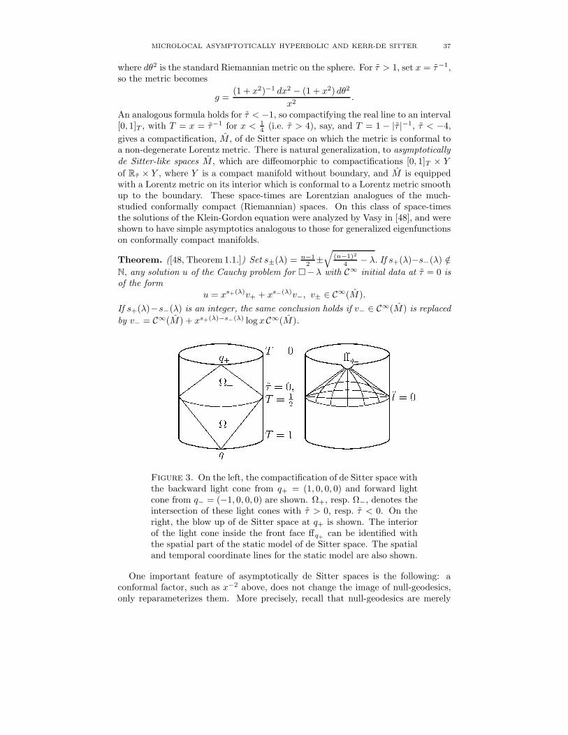
MICROLOCAL ASYMPTOTICALLY HYPERBOLIC AND KERR-DE SITTER 37
where dθ2 is the standard Riemannian metric on the sphere. For τ > 1, set x = τ−1,so the metric becomes
g =(1 + x2)−1 dx2 − (1 + x2) dθ2
x2.
An analogous formula holds for τ < −1, so compactifying the real line to an interval[0, 1]T , with T = x = τ−1 for x < 1
4 (i.e. τ > 4), say, and T = 1 − |τ |−1, τ < −4,
gives a compactification, M, of de Sitter space on which the metric is conformal toa non-degenerate Lorentz metric. There is natural generalization, to asymptoticallyde Sitter-like spaces M , which are diffeomorphic to compactifications [0, 1]T × Y
of Rτ × Y , where Y is a compact manifold without boundary, and M is equippedwith a Lorentz metric on its interior which is conformal to a Lorentz metric smoothup to the boundary. These space-times are Lorentzian analogues of the much-studied conformally compact (Riemannian) spaces. On this class of space-timesthe solutions of the Klein-Gordon equation were analyzed by Vasy in [48], and wereshown to have simple asymptotics analogous to those for generalized eigenfunctionson conformally compact manifolds.
Theorem. ([48, Theorem 1.1.]) Set s±(λ) = n−12 ±
√(n−1)2
4 − λ. If s+(λ)−s−(λ) /∈N, any solution u of the Cauchy problem for −λ with C∞ initial data at τ = 0 isof the form
u = xs+(λ)v+ + xs−(λ)v−, v± ∈ C∞(M).
If s+(λ)−s−(λ) is an integer, the same conclusion holds if v− ∈ C∞(M) is replaced
by v− = C∞(M) + xs+(λ)−s−(λ) log x C∞(M).
Figure 3. On the left, the compactification of de Sitter space withthe backward light cone from q+ = (1, 0, 0, 0) and forward lightcone from q− = (−1, 0, 0, 0) are shown. Ω+, resp. Ω−, denotes theintersection of these light cones with τ > 0, resp. τ < 0. On theright, the blow up of de Sitter space at q+ is shown. The interiorof the light cone inside the front face ffq+
can be identified withthe spatial part of the static model of de Sitter space. The spatialand temporal coordinate lines for the static model are also shown.
One important feature of asymptotically de Sitter spaces is the following: aconformal factor, such as x−2 above, does not change the image of null-geodesics,only reparameterizes them. More precisely, recall that null-geodesics are merely
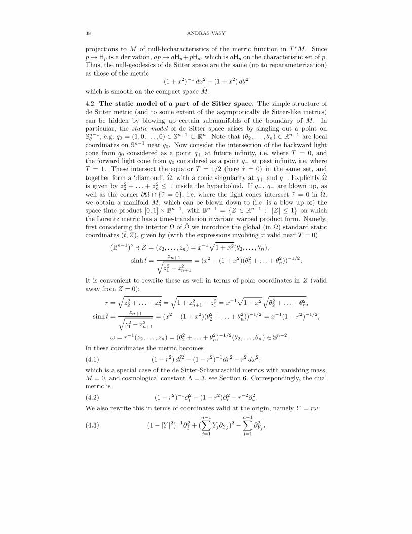
38 ANDRAS VASY
projections to M of null-bicharacteristics of the metric function in T ∗M . Sincep 7→ Hp is a derivation, ap 7→ aHp +pHa, which is aHp on the characteristic set of p.Thus, the null-geodesics of de Sitter space are the same (up to reparameterization)as those of the metric
(1 + x2)−1 dx2 − (1 + x2) dθ2
which is smooth on the compact space M .
4.2. The static model of a part of de Sitter space. The simple structure ofde Sitter metric (and to some extent of the asymptotically de Sitter-like metrics)
can be hidden by blowing up certain submanifolds of the boundary of M . Inparticular, the static model of de Sitter space arises by singling out a point onS
n−1θ , e.g. q0 = (1, 0, . . . , 0) ∈ Sn−1 ⊂ Rn. Note that (θ2, . . . , θn) ∈ Rn−1 are local
coordinates on Sn−1 near q0. Now consider the intersection of the backward lightcone from q0 considered as a point q+ at future infinity, i.e. where T = 0, andthe forward light cone from q0 considered as a point q− at past infinity, i.e. whereT = 1. These intersect the equator T = 1/2 (here τ = 0) in the same set, and
together form a ‘diamond’, Ω, with a conic singularity at q+ and q−. Explicitly Ωis given by z2
2 + . . . + z2n ≤ 1 inside the hyperboloid. If q+, q− are blown up, as
well as the corner ∂Ω ∩ τ = 0, i.e. where the light cones intersect τ = 0 in Ω,we obtain a manifold M , which can be blown down to (i.e. is a blow up of) thespace-time product [0, 1] × Bn−1, with Bn−1 = Z ∈ Rn−1 : |Z| ≤ 1 on whichthe Lorentz metric has a time-translation invariant warped product form. Namely,first considering the interior Ω of Ω we introduce the global (in Ω) standard staticcoordinates (t, Z), given by (with the expressions involving x valid near T = 0)
(Bn−1) 3 Z = (z2, . . . , zn) = x−1√
1 + x2(θ2, . . . , θn),
sinh t =zn+1√
z21 − z2
n+1
= (x2 − (1 + x2)(θ22 + . . . + θ2
n))−1/2.
It is convenient to rewrite these as well in terms of polar coordinates in Z (validaway from Z = 0):
r =√
z22 + . . . + z2
n =√
1 + z2n+1 − z2
1 = x−1√
1 + x2
√θ22 + . . . + θ2
n,
sinh t =zn+1√
z21 − z2
n+1
= (x2 − (1 + x2)(θ22 + . . . + θ2
n))−1/2 = x−1(1 − r2)−1/2,
ω = r−1(z2, . . . , zn) = (θ22 + . . . + θ2
n)−1/2(θ2, . . . , θn) ∈ Sn−2.
In these coordinates the metric becomes
(4.1) (1 − r2) dt2 − (1 − r2)−1dr2 − r2 dω2,
which is a special case of the de Sitter-Schwarzschild metrics with vanishing mass,M = 0, and cosmological constant Λ = 3, see Section 6. Correspondingly, the dualmetric is
(4.2) (1 − r2)−1∂2t − (1 − r2)∂2
r − r−2∂2ω .
We also rewrite this in terms of coordinates valid at the origin, namely Y = rω:
(4.3) (1 − |Y |2)−1∂2t + (
n−1∑
j=1
Yj∂Yj)2 −
n−1∑
j=1
∂2Yj
.
MICROLOCAL ASYMPTOTICALLY HYPERBOLIC AND KERR-DE SITTER 39
4.3. Blow-up of the static model. We have already seen that de Sitter spacehas a smooth conformal compactification; the singularities in the metric of the form(4.1) at r = 1 must thus be artificial. On the other hand, the metric is alreadywell-behaved for r < 1 bounded away from 1, so we want the coordinate change tobe smooth there — this means smoothness in valid coordinates (Y above) at theorigin as well. This singularity can be removed by a blow-up on an appropriatecompactification. We phrase this at first in a way that is closely related to ourtreatment of Kerr-de Sitter space, and the Kerr-star coordinates. So let
t = t + h(r), h(r) = −1
2log µ, µ = 1 − r2.
Note that h is smooth at the origin, A key feature of this change of coordinates is
h′(r) = − r
µ= − 1
µ+
1
1 + r,
which is −µ−1 near r = 1 modulo terms smooth at r = 1. Other coordinate changeswith this property would also work. Let
τ = e−t =e−t
µ1/2.
Thus, if we compactify static space-time as Bn−1rω × [0, 1]T , with T = τ for say t > 4,
then this procedure amounts to blowing up T = 0, µ = 0 parabolically. (If we usedτ = e−2t, everything would go through, except there would be many additionalfactors of 2; then the blow-up would be homogeneous, i.e. spherical.) Then thedual metric becomes
−µ∂2r − 2r∂rτ∂τ + τ2∂2
τ − r−2∂2ω ,
or
−4r2µ∂2µ + 4r2τ∂τ∂µ + τ2∂2
τ − r−2∂2ω,
which is a non-degenerate Lorentzian b-metric19 on Rn−1rω × [0, 1)τ , i.e. it extends
smoothly and non-degenerately across the ‘event horizon’, r = 1. Note that incoordinates valid near r = 0 this becomes
(∑
j
Yj∂Yj)2 − 2(
∑
j
Yj∂Yj)τ∂τ + τ2∂2
τ −∑
j
∂2Yj
= (τ∂τ −∑
j
Yj∂Yj)2 −
∑
j
∂2Yj
.
In slightly different notation, this agrees with the symbol of [48, Equation (7.3)].
We could have used other equivalent local coordinates; for instance replaced e−t
by (sinh t)−1, in which case the coordinates (r, τ, ω) we obtained are replaced by
(4.4) r, ρ = (sinh t)−1/(1 − r2)1/2 = x, ω.
As expected, in these coordinates the metric would still be a smooth and non-degenerate b-metric. These coordinates also show that Kerr-star-type coordinatesare smooth in the interior of the front face on the blow-up of our conformal com-pactification of de Sitter space at q+. 20 In summary we have reproved (modulo afew details):
19See Section 3 for a quick introduction to b-geometry and further references.20If we had worked with e−2t instead of e−t above, we would obtain x2 as the defining function
of the temporal face, rather than x.
40 ANDRAS VASY
Lemma 4.1. (See [36, Lemma 2.1] for a complete version.) The lift of Ω to the
blow up [M ; q+, q−] is a C∞ manifold with corners, Ω. Moreover, near the frontfaces ffq± , Ω is naturally diffeomorphic to a neighborhood of the temporal faces
tf± in the C∞ manifold with corners obtained from [0, 1]T × Bn−1 by blowing up0× ∂Bn−1 and 1× ∂Bn−1 in the parabolic manner indicated in (4.4); here tf±are the lifts of 0 × ∂Bn−1 and 1 × ∂Bn−1.
It is worthwhile comparing the de Sitter space wave asymptotics of [48],
(4.5) u = xn−1v+ + v−, v+ ∈ C∞(M), v− ∈ C∞(M) + xn−1(log x)C∞(M),
with our main result, Theorem 1.4. The fact that the coefficients in the de Sitterexpansion are C∞ on M means that on M , the leading terms are constant. Thus,(4.5) implies (and is much stronger than) the statement that u decays to a constanton M at an exponential rate.
4.4. D’Alembertian and its Mellin transform. Consider the d’Alembertian,g, whose principal symbol, including subprincipal terms, is given by the metricfunction. Thus, writing b-covectors as
ξ dµ + σdτ
τ+ η dω,
we have
(4.6) G = σb,2() = −4r2µξ2 + 4r2σξ + σ2 − r−2|η|2,
with |η|2ω denoting the dual metric function on the sphere. Note that there is a polarcoordinate singularity at r = 0; this is resolved by using actually valid coordinatesY = rω on Rn−1 near the origin; writing b-covectors as
σdτ
τ+ ζ dY,
we have
G = σb,2() = (Y · ζ)2 − 2(Y · ζ)σ + σ2 − |ζ|2 = (Y · ζ − σ)2 − |ζ|2,Y · ζ =
∑
j
Yj · ζj , |ζ|2 =∑
j
ζ2j .(4.7)
Since there are no interesting phenomena at the origin, we may ignore this pointbelow.
Via conjugation by the (inverse) Mellin transform, see Subsection 3.1, we obtain afamily of operators Pσ depending on σ on Rn−1
rω with both principal and high energy(|σ| → ∞) symbol given by (4.6). Thus, the principal symbol of Pσ ∈ Diff2(Rn−1),including in the high energy sense (σ → ∞), is
pfull = −4r2µξ2 + 4r2σξ + σ2 − r−2|η|2ω= (Y · ζ)2 − 2(Y · ζ)σ + σ2 − |ζ|2 = (Y · ζ − σ)2 − |ζ|2.
(4.8)
The Hamilton vector field is
Hpfull= 4r2(−2µξ + σ)∂µ − r−2
H|η|2ω− (4(1 − 2r2)ξ2 − 4σξ − r−4|η|2ω)∂ξ
= 2(Y · ζ − σ)(Y · ∂Y − ζ · ∂ζ) − 2ζ · ∂Y ,(4.9)
MICROLOCAL ASYMPTOTICALLY HYPERBOLIC AND KERR-DE SITTER 41
with ζ ·∂Y =∑
ζj∂Yj, etc. Thus, in the standard ‘classical’ sense, which effectively
means letting σ = 0, the principal symbol is
p = σ2(Pσ) = −4r2µξ2 − r−2|η|2ω= (Y · ζ)2 − |ζ|2,
(4.10)
while the Hamilton vector field is
Hp = −8r2µξ∂µ − r−2H|η|2ω
− (4(1 − 2r2)ξ2 − r−4|η|2ω)∂ξ
= 2(Y · ζ)(Y · ∂Y − ζ · ∂ζ) − 2ζ · ∂Y ,(4.11)
Moreover, the imaginary part of the subprincipal symbol, given by the principalsymbol of 1
2ı (Pσ − P ∗σ ), is
σ1(1
2ı(Pσ − P ∗
σ )) = 4r2(Im σ)ξ = −2(Y · ζ) Im σ.
When comparing these with [48, Section 7], it is important to keep in mind thatwhat is denoted by σ there (which we refer to as σ here to avoid confusion) is ıσhere corresponding to the Mellin transform, which is a decomposition in terms ofτ ıσ ∼ xıσ , being replaced by weights xσ in [48, Equation (7.4)].
One important feature of this operator is that
N∗µ = 0 = (µ, ω, ξ, η) : µ = 0, η = 0is invariant under the classical flow (i.e. effectively letting σ = 0). Let
N∗S \ o = Λ+ ∪ Λ−, Λ± = N∗S ∩ ±ξ > 0, S = µ = 0.Let L± be the image of Λ± in S∗Rn−1. Next we analyze the flow at Λ±. First,
(4.12) Hp|η|2ω = 0
and
(4.13) Hpµ = −8r2µξ = −8ξµ + aµξ
with a being C∞ in T ∗X , and homogeneous of degree 0. While, in the spirit oflinearizations, we used an expression in (4.13) that is linear in the coordinateswhose vanishing defines N∗S, the key point is that µ is an elliptic multiple of p ina linearization sense, so one can simply use p = p/|ξ|2 (which is homogeneous ofdegree 0, like µ), in its place.
It is convenient to rehomogenize (4.12) in terms of η = η/|ξ|. To phrase this
more invariantly, consider the fiber-compactification T∗Rn−1 of T ∗Rn−1, see Sub-
section 2.2. On this space, the classical principal symbol, p, is (essentially) a func-
tion on ∂T∗Rn−1 = S∗Rn−1. Then at fiber infinity near N∗S, we can take (|ξ|−1, η)
as coordinates on the fibers of the cotangent bundle, with ρ = |ξ|−1 defining S∗X
in T∗X . Then |ξ|−1
Hp is a C∞ vector field in this region and
(4.14) |ξ|−1Hp|η|2 = |η|2Hp|ξ|−1 = −4(sgn ξ)|η|2 + a,
where a vanishes cubically at N∗S, i.e. (2.3) holds. In similar notation we have
Hp|ξ|−1 = −4 sgn(ξ) + a′,
|ξ|−1Hpµ = −8(sgn ξ)µ.
(4.15)
with a′ smooth (indeed, homogeneous degree zero without the compactification)vanishing at N∗S. As the vanishing of η, |ξ|−1 and µ defines ∂N∗S, we con-clude that L− = ∂Λ− is a source, while L+ = ∂Λ+ is a sink, in the sense that
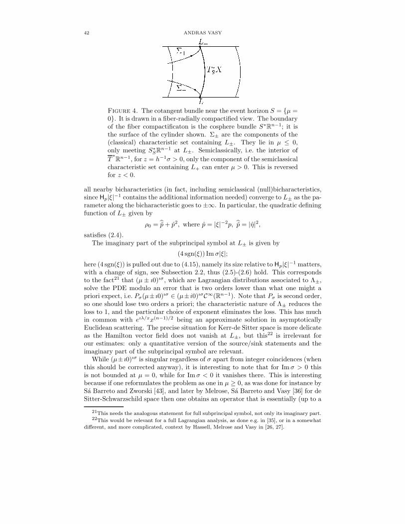
42 ANDRAS VASY
Figure 4. The cotangent bundle near the event horizon S = µ =0. It is drawn in a fiber-radially compactified view. The boundaryof the fiber compactificaton is the cosphere bundle S∗Rn−1; it isthe surface of the cylinder shown. Σ± are the components of the(classical) characteristic set containing L±. They lie in µ ≤ 0,only meeting S∗
SRn−1 at L±. Semiclassically, i.e. the interior of
T∗Rn−1, for z = h−1σ > 0, only the component of the semiclassical
characteristic set containing L+ can enter µ > 0. This is reversedfor z < 0.
all nearby bicharacteristics (in fact, including semiclassical (null)bicharacteristics,since Hp|ξ|−1 contains the additional information needed) converge to L± as the pa-rameter along the bicharacteristic goes to ±∞. In particular, the quadratic definingfunction of L± given by
ρ0 = p + p2, where p = |ξ|−2p, p = |η|2,satisfies (2.4).
The imaginary part of the subprincipal symbol at L± is given by
(4 sgn(ξ)) Im σ|ξ|;here (4 sgn(ξ)) is pulled out due to (4.15), namely its size relative to Hp|ξ|−1 matters,with a change of sign, see Subsection 2.2, thus (2.5)-(2.6) hold. This correspondsto the fact21 that (µ ± ı0)ıσ , which are Lagrangian distributions associated to Λ±,solve the PDE modulo an error that is two orders lower than what one might apriori expect, i.e. Pσ(µ± ı0)ıσ ∈ (µ± i0)ıσC∞(Rn−1). Note that Pσ is second order,so one should lose two orders a priori; the characteristic nature of Λ± reduces theloss to 1, and the particular choice of exponent eliminates the loss. This has muchin common with eıλ/xx(n−1)/2 being an approximate solution in asymptoticallyEuclidean scattering. The precise situation for Kerr-de Sitter space is more delicateas the Hamilton vector field does not vanish at L±, but this22 is irrelevant forour estimates: only a quantitative version of the source/sink statements and theimaginary part of the subprincipal symbol are relevant.
While (µ± ı0)ıσ is singular regardless of σ apart from integer coincidences (whenthis should be corrected anyway), it is interesting to note that for Im σ > 0 thisis not bounded at µ = 0, while for Im σ < 0 it vanishes there. This is interestingbecause if one reformulates the problem as one in µ ≥ 0, as was done for instance bySa Barreto and Zworski [43], and later by Melrose, Sa Barreto and Vasy [36] for deSitter-Schwarzschild space then one obtains an operator that is essentially (up to a
21This needs the analogous statement for full subprincipal symbol, not only its imaginary part.22This would be relevant for a full Lagrangian analysis, as done e.g. in [35], or in a somewhat
different, and more complicated, context by Hassell, Melrose and Vasy in [26, 27].
MICROLOCAL ASYMPTOTICALLY HYPERBOLIC AND KERR-DE SITTER 43
conjugation and a weight, see below) the Laplacian on an asymptotically hyperbolic
space at energy σ2 + (n−2)2
4 — more precisely its normal operator (which encodesits behavior near µ = 0) is a multiple of that of the hyperbolic Laplacian. Then thegrowth/decay behavior corresponds to the usual scattering theory phenomena, butin our approach smooth extendability across µ = 0 is the distinguishing feature ofthe solutions we want, not growth/decay. See Remark 4.5 for more details.
4.5. Global behavior of the characteristic set. First remark that 〈 dττ , dτ
τ 〉G =
1 > 0, so dττ is time-like. Correspondingly all the results of Subsection 3.2 apply. In
particular, (3.14) gives that the characteristic set is divided into two componentswith Λ± in different components. It is easy to make this explicit: points with ξ = 0,or equivalently Y · ζ = 0, cannot lie in the characteristic set. Thus,
Σ± = Σ ∩ ±ξ > 0 = Σ ∩ ∓(Y · ζ) > 0.While it is not important here since the characteristic set in µ ≥ 0 is localized at
N∗S, hence one has a similar localization for nearby µ, for global purposes (whichwe do not need here), we point out that Hpµ = −8r2µξ. Since ξ 6= 0 on Σ, and inΣ, r = 1 can only happen at N∗S, i.e. only at the radial set, the C∞ function µprovides a positive global escape function which is increasing on Σ+, decreasing onΣ−. Correspondingly, bicharacteristics in Σ+ travel from infinity to L+, while inΣ− they travel from L− to infinity.
4.6. High energy, or semiclassical, asymptotics. We are also interested in thehigh energy behavior, as |σ| → ∞. For the associated semiclassical problem oneobtains a family of operators
Ph,z = h2Ph−1z,
with h = |σ|−1, and z corresponding to σ/|σ| in the unit circle in C. Then thesemiclassical principal symbol p~,z of Ph,z is a function on T ∗Rn−1. As in Section 2,we are interested in Im z ≥ −Ch, which corresponds to Im σ ≥ −C. It is sometimesconvenient to think of p~,z, and its rescaled Hamilton vector field, as objects on
T∗Rn−1. Thus,
p~,z = σ2,h(Ph,z) = −4r2µξ2 + 4r2zξ + z2 − r−2|η|2ω= (Y · ζ)2 − 2(Y · ζ)z + z2 − |ζ|2 = (Y · ζ − z)2 − |ζ|2.
(4.16)
We make the general discussion of Subsection 3.2 explicit. First,
(4.17) Im p~,z = 2 Im z(2r2ξ + Re z) = −2 Im z(Y · ζ − Re z).
In particular, for z non-real, Im p~,z = 0 implies 2r2ξ+Re z = 0, i.e. Y ·ζ−Re z = 0,which means that Re p~,z is
(4.18) −r−2(Re z)2 − (Im z)2 − r−2|η|2ω = −(Im z)2 − |ζ|2 < 0,
i.e. p~,z is semiclassically elliptic on T ∗Rn−1, but not at fiber infinity, i.e. at S∗Rn−1
(standard ellipticity is lost only in r ≥ 1, of course). Explicitly, if we introduce forinstance
(µ, ω, ν, η), ν = |ξ|−1, η = η/|ξ|,as valid projective coordinates in a (large!) neighborhood of L± in T
∗Rn−1, then
ν2p~,z = −4r2µ + 4r2(sgn ξ)zν + z2ν2 − r−2|η|2ω
44 ANDRAS VASY
soν2 Im p~,z = 4r2(sgn ξ)ν Im z + 2ν2 Re z Im z
which automatically vanishes at ν = 0, i.e. at S∗Rn−1. Thus, for σ large and pureimaginary, the semiclassical problem adds no complexity to the ‘classical’ quantumproblem, but of course it does not simplify it. In fact, we need somewhat moreinformation at the characteristic set, which is thus at ν = 0 when Im z is boundedaway from 0:
ν small, Im z ≥ 0 ⇒ (sgn ξ) Im p~,z ≥ 0 ⇒ ± Im p~,z ≥ 0 near Σ~,±,
ν small, Im z ≤ 0 ⇒ (sgn ξ) Im p~,z ≤ 0 ⇒ ± Im p~,z ≥ 0 near Σ~,±,
which, as we have seen, means that for Ph,z with Im z > 0 one can propagateestimates forwards along the bicharacteristics where ξ < 0 (in particular, awayfrom L−, as the latter is a source) and backwards where ξ > 0 (in particular,away from L+, as the latter is a sink), while for P ∗
h,z the directions are reversed.The directions are also reversed if Im z switches sign. This is important because itgives invertibility for z = ı (corresponding to Im σ large positive, i.e. the physicalhalfplane), but does not give invertibility for z = −ı negative.
We now return to the claim that even semiclassically, for z almost real23, thecharacteristic set can be divided into two components Σ~,±, with L± in differentcomponents. As explained in Subsection 3.2 the vanishing of the factor followingIm z in (4.17) gives a hypersurface that separates Σ~ into two parts; this can beeasily checked also by a direct computation. Concretely, this is the hypersurfacegiven by
(4.19) 0 = 2r2ξ + Re z = −(Y · ζ − Re z),
and soΣ~,± = Σ~ ∩ ∓(Y · ζ − Re z) > 0.
We finally need more information about the global semiclassical dynamics. Hereall null-bicharacteristics go to either L+ in the forward direction or to L− in thebackward direction, and escape to infinity in the other direction. Rather thanproving this at once, which depends on the global non-trapping structure on Rn−1,we first give an argument that is local near the event horizon, and suffices for theextension discussed below for asymptotically hyperbolic spaces.
As stated above, first, we are only concerned about semiclassical dynamics inµ > µ0, where µ0 < 0 might be close to 0. To analyze this, we observe that thesemiclassical Hamilton vector field is
Hp~,z= 4r2(−2µξ + z)∂µ − r−2
H|η|2ω− (4(1 − 2r2)ξ2 − 4zξ − r−4|η|2ω)∂ξ
= 2(Y · ζ − z)(Y · ∂Y − ζ · ∂ζ) − 2ζ · ∂Y ;(4.20)
here we are concerned about z real. Thus,
Hp~,z(Y · ζ) = −2|ζ|2,
and ζ = 0 implies p~,z = z2, so Hp~,z(Y · ζ) has a negative upper bound on the
characteristic set in compact subsets of T ∗r < 1; note that the characteristic set iscompact in T ∗r ≤ r0 if r0 < 1 by standard ellipticity. Thus, bicharacteristics haveto leave r ≤ r0 for r0 < 1 in both the forward and backward direction (as Y · ζ isbounded over this region on the characteristic set). We already know the dynamics
23So the operator is not semiclassically elliptic on T ∗Rn−1; as mentioned above, for Im z
uniformly bounded away from R, we have ellipticity in T ∗Rn−1.
MICROLOCAL ASYMPTOTICALLY HYPERBOLIC AND KERR-DE SITTER 45
near L±, which is the only place where the characteristic set intersects S∗SRn−1,
namely L+ is a sink and L− is a source. Now, at µ = 0, Hp~,zµ = z, which is positive
when z > 0, so bicharacteristics can only cross µ = 0 in the inward direction. Inview of our preceding observations, thus, once a bicharacteristic crossed µ = 0, ithas to tend to L+. As bicharacteristics in a neighborhood of L+ (even in µ < 0)tend to L+ since L+ is a sink, it follows that in Σ~,+ the same is true in µ > µ0
for some µ0 < 0. On the other hand, in a neighborhood of L− all bicharacteristicsemanate from L− (but cannot cross into µ > 0 by our observations), so leave µ > µ0
in the forward direction. These are all the relevant features of the bicharacteristicflow for our purposes as we shall place a complex absorbing potential near µ = µ0
in the next subsection.However, it is easy to see the global claim by noting that Hp~,z
µ = 4r2(−2µξ+z),and this cannot vanish on Σ~ in µ < 0, since where it vanishes, a simple calculationgives p~,z = 4µξ2 − r−2|η|2. Thus, Hp~,z
µ has a constant sign on Σ~,± in µ < 0,so combined with the observation above that all bicharacteristics escape to µ = µ0
in the appropriate direction, it shows that all bicharacteristics in fact escape toinfinity in that direction24.
In fact, for applications, it is also useful to remark that for α ∈ T ∗X ,
(4.22) 0 < µ(α) < 1, p~,z(α) = 0 and (Hp~,zµ)(α) = 0 ⇒ (H2
p~,zµ)(α) < 0.
Indeed, as Hp~,zµ = 4r2(−2µξ + z), the hypotheses imply z = 2µξ and H
2p~,z
µ =
−8r2µHp~,zξ, so we only need to show that Hp~,z
ξ > 0 at these points. Since
Hp~,zξ = −4(1 − 2r2)ξ2 + 4zξ + r−4|η|2ω = 4ξ2 + r−4|η|2ω = 4r−2ξ2,
where the second equality uses Hp~,zµ = 0 and the third uses that in addition
p~,z = 0, this follows from 2µξ = z 6= 0, so ξ 6= 0. Thus, µ can be used for gluingconstructions as in [13].
4.7. Complex absorption. The final step of fitting Pσ into our general microlocalframework is moving the problem to a compact manifold, and adding a complexabsorbing second order operator. We thus consider a compact manifold withoutboundary X for which Xµ0
= µ > µ0, µ0 < 0, say, is identified as an open subsetwith smooth boundary; it is convenient to take X to be the double25 of Xµ0
.
24There is in fact a not too complicated global escape function, e.g.
f =2Y · ζ − Re z
2p
1 + |Y |2(Y · ζ − Re z)=
2Y · ζ − Re z|ζ|−1
2p
1 + |Y |2(Y · ζ − Re z|ζ|−1),
which is a smooth function on the characteristic set in T ∗Rn−1 as Y · ζ 6= Re z there; further,
it extends smoothly to the characteristic set in T∗Rn−1 away from L± since
p
1 + |Y |2(Y · ζ −Re z|ζ|−1) vanishes only there near S∗Rn−1 (where these are valid coordinates), at which it hasconic points. This function arises in a straightforward manner when one reduces Minkowski space,Rn = R
n−1z′ × Rt with metric g0, to the boundary of its radial compactification, as described in
Section 5, and uses the natural escape function
(4.21) f =tt∗ − z′(z′)∗
t∗p
t2 + |z′|2
there; here t∗ is the dual variable of t and (z′)∗ of z′, outside the origin.25In fact, in the de Sitter context, this essentially means moving to the boundary of n-
dimensional Minkowski space, where our (n − 1)-dimensional model is the ‘upper hemisphere’,see Section 5. Thus, doubling over means working with the whole boundary, but putting an ab-sorbing operator near the equator, corresponding to the usual Cauchy hypersurface in Minkowski
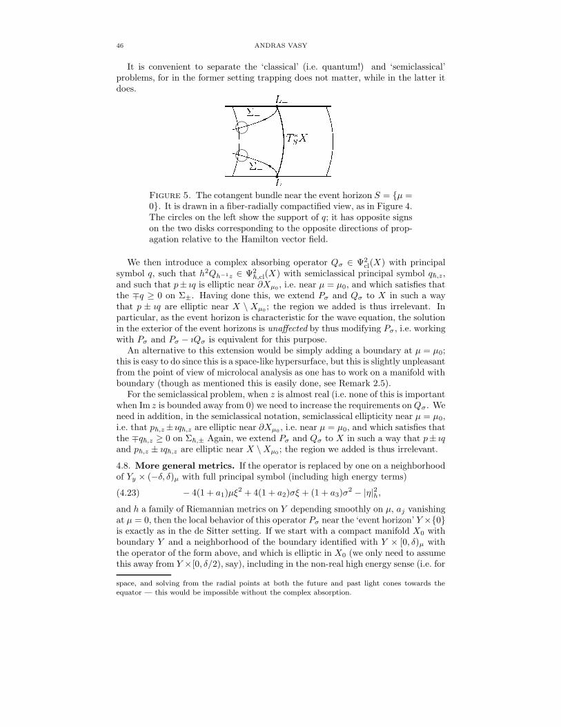
46 ANDRAS VASY
It is convenient to separate the ‘classical’ (i.e. quantum!) and ‘semiclassical’problems, for in the former setting trapping does not matter, while in the latter itdoes.
Figure 5. The cotangent bundle near the event horizon S = µ =0. It is drawn in a fiber-radially compactified view, as in Figure 4.The circles on the left show the support of q; it has opposite signson the two disks corresponding to the opposite directions of prop-agation relative to the Hamilton vector field.
We then introduce a complex absorbing operator Qσ ∈ Ψ2cl(X) with principal
symbol q, such that h2Qh−1z ∈ Ψ2~,cl(X) with semiclassical principal symbol q~,z,
and such that p± ıq is elliptic near ∂Xµ0, i.e. near µ = µ0, and which satisfies that
the ∓q ≥ 0 on Σ±. Having done this, we extend Pσ and Qσ to X in such a waythat p ± ıq are elliptic near X \ Xµ0
; the region we added is thus irrelevant. Inparticular, as the event horizon is characteristic for the wave equation, the solutionin the exterior of the event horizons is unaffected by thus modifying Pσ , i.e. workingwith Pσ and Pσ − ıQσ is equivalent for this purpose.
An alternative to this extension would be simply adding a boundary at µ = µ0;this is easy to do since this is a space-like hypersurface, but this is slightly unpleasantfrom the point of view of microlocal analysis as one has to work on a manifold withboundary (though as mentioned this is easily done, see Remark 2.5).
For the semiclassical problem, when z is almost real (i.e. none of this is importantwhen Im z is bounded away from 0) we need to increase the requirements on Qσ . Weneed in addition, in the semiclassical notation, semiclassical ellipticity near µ = µ0,i.e. that p~,z ± ıq~,z are elliptic near ∂Xµ0
, i.e. near µ = µ0, and which satisfies thatthe ∓q~,z ≥ 0 on Σ~,± Again, we extend Pσ and Qσ to X in such a way that p± ıqand p~,z ± ıq~,z are elliptic near X \ Xµ0
; the region we added is thus irrelevant.
4.8. More general metrics. If the operator is replaced by one on a neighborhoodof Yy × (−δ, δ)µ with full principal symbol (including high energy terms)
− 4(1 + a1)µξ2 + 4(1 + a2)σξ + (1 + a3)σ2 − |η|2h,(4.23)
and h a family of Riemannian metrics on Y depending smoothly on µ, aj vanishingat µ = 0, then the local behavior of this operator Pσ near the ‘event horizon’ Y ×0is exactly as in the de Sitter setting. If we start with a compact manifold X0 withboundary Y and a neighborhood of the boundary identified with Y × [0, δ)µ withthe operator of the form above, and which is elliptic in X0 (we only need to assumethis away from Y ×[0, δ/2), say), including in the non-real high energy sense (i.e. for
space, and solving from the radial points at both the future and past light cones towards theequator — this would be impossible without the complex absorption.
MICROLOCAL ASYMPTOTICALLY HYPERBOLIC AND KERR-DE SITTER 47
z away from R when σ = h−1z) then we can extend the operator smoothly to oneon Xµ0
, µ0 = −δ, which enjoys all the properties above, except semiclassical non-trapping. If we assume that X
0 is non-trapping in the usual sense, the semiclassicalnon-trapping property also follows. In addition, for µ > 0 sufficiently small, (4.22)also holds since η is small when Hp~,z
µ = 0 and p~,z = 0, for the former gives
z = 2(1 + a2)−1(1 + a1)µξ, and then the latter gives
4(1 + a1)
(1 +
(1 + a1)(1 + a3)
(1 + a2)2µ
)µξ2 = |η|2h,
so the contribution of |η|2h to Hp~,zξ, which can be large elsewhere even at µ = 0,
is actually small.
4.9. Results. The preceding subsections show that for the Mellin transform of g
on n-dimensional de Sitter space, all the hypotheses needed in Section 2 are satisfied,thus analogues of the results stated for Kerr-de Sitter space in the introduction,Theorems 1.1-1.4, hold. It is important to keep in mind, however, that there is notrapping to remove, so Theorem 1.1 applies with Qσ supported outside the eventhorizon, and one does not need gluing or the result of Wunsch and Zworski [52].In particular, Theorem 1.3 holds with arbitrary C ′, without the logarithmic orpolynomial loss. As already mentioned when discussing [48, Theorem 1.1] at thebeginning of this section, this is weaker than the result of [48, Theorem 1.1], sincethere one has smooth asymptotics without a blow-up of a boundary point26.
We now reinterpret our results on the Mellin transform side in terms of (n− 1)-dimensional hyperbolic space. Let B
n−11/2 be Bn−1 = r ≤ 1 with ν =
õ added
to the smooth structure. For the purposes of the discussion below, we identify theinterior r < 1 of B
n−11/2 with the Poincare ball model of hyperbolic (n − 1)-space
(Hn−1, gHn−1). Using polar coordinates around the origin, let cosh ρ = ν−1, ρ isthe distance from the origin. The Laplacian on Hn−1 in these coordinates is
∆Hn−1 = D2ρ − ı(n − 2) coth ρ Dρ + (sinh ρ)−2∆ω.
It is shown in [48, Lemma 7.10] that in r < 1, and with s be such that 2s = ıσ− n2 ,
(1 − r2)−sPσ(1 − r2)s = νn2−ıσPσνıσ− n
2
= −ν−1
(∆Hn−1 − σ2 −
(n − 2
2
)2
− ν2 n(n − 2)
4
)ν−1
= − cosh ρ
(∆Hn−1 − σ2 −
(n − 2
2
)2
− (cosh ρ)−2 n(n − 2)
4
)cosh ρ.
(4.24)
We thus deduce:
Proposition 4.2. The inverse R(σ) of
∆Hn−1 − σ2 −(
n − 2
2
)2
− (cosh ρ)−2 n(n − 2)
4
26Note that our methods work equally well for asymptotically de Sitter spaces in the sense of[48]; after the blow up, the boundary metric is ‘frozen’ at the point that is blown up, hence theinduced problem at the front face is the same as for the de Sitter metric with asymptotics givenby this ‘frozen’ metric.
48 ANDRAS VASY
has a meromorphic continuation from Im σ > 0 to C with poles with finite rankresidues as a map R(σ) : C∞(Bn−1) → C−∞(Bn−1), and with non-trapping esti-mates in every strip | Im σ| < C, |Re σ| 0: s > 1
2 + C,(4.25)
‖(cosh ρ)(n−2)/2−ıσR(σ)f‖Hs
|σ|−1(Bn−1) ≤ C|σ|−1‖(cosh ρ)(n+2)/2−ıσf‖Hs−1
|σ|−1(Bn−1),
where the Sobolev spaces are those on Bn−1 (rather than Bn−11/2 ). If supp f ⊂
(Bn−1), the s − 1 norm on f can be replaced by the s − 2 norm.The same conclusion holds for small even C∞ perturbations, vanishing at ∂B
n−11/2 ,
of gHn−1 in the class of conformally compact metrics, or the addition of (not nec-essarily small) V ∈ µC∞(Bn−1).
Proof. By self-adjointness and positivity of ∆Hn−1 ,(
∆Hn−1 − σ2 −(
n − 2
2
)2
− ν2 n(n − 2)
4
)u = f ∈ C∞(Bn−1)
has a unique solution u = R(σ)f ∈ L2(Bn−11/2 , |dgHn−1 |) when when Im σ 0. On
the other hand, let f0 = νıσ−n/2ν−1f in r ≤ 1, and f0 still vanishes to infinite orderat r = 1. Let f be an arbitrary smooth extension of f0 to the compact manifoldX on which Pσ − ıQσ is defined. Let u = (Pσ − ıQσ)−1f , with (Pσ − ıQσ)−1 given
by our results in Section 2; this satisfies (Pσ − ıQσ)u = f and u ∈ C∞(X). Thus,u′ = ν−ıσ+n/2ν−1u|r<1 satisfies u′ ∈ ν(n−2)/2−ıσC∞(Bn−1), and
(∆Hn−1 − σ2 −
(n − 2
2
)2
− ν2 n(n − 2)
4
)u′ = f
by (4.24) (as Qσ is supported in r > 1). Since u′ ∈ L2(Bn−1, |dgHn−1 |) for Im σ > 0,by the aforementioned uniqueness, u = u′.
To make the extension from Bn−1 to X more systematic, let Es : Hs(Bn−1) →Hs(X) be a continuous extension operator, Rs : Hs(X) → Hs(Bn−1) the restriction
map. Then, as we have just seen, for f ∈ C∞(Bn−1),
(4.26) R(σ)f = ν−ıσ+n/2ν−1Rs(Pσ − ıQσ)−1Es−1νıσ−n/2ν−1f.
Thus, the first half of the proposition (including the non-trapping estimate) followsimmediately from the results of Section 2. Note also that this proves that every poleof R(σ) is a pole of (Pσ − ıQσ)−1 (for otherwise (4.26) would show R(σ) does nothave a pole either), but it is possible for (Pσ − ıQσ)−1 to have poles which are notpoles of R(σ). However, in the latter case, the Laurent coefficients of (Pσ − ıQσ)−1
would be annihilated by multiplication by Rs from the left, i.e. the resonant states(which are smooth) would be supported in µ ≤ 0, in particular vanish to infiniteorder at µ = 0.
In fact, a stronger statement can be made: by a calculation completely analogousto what we just performed, we can easily see that in µ < 0, Pσ is a conjugate (timesa power of µ) of a Klein-Gordon-type operator on (n−1)-dimensional de Sitter spacewith µ = 0 being the boundary (i.e. where time goes to infinity). Thus, if σ is nota pole of R(σ) and (Pσ − ıQσ)u = 0 then one would have a solution u of this Klein-Gordon-type equation near µ = 0, i.e. infinity, that rapidly vanishes at infinity.It is shown in [48, Proposition 5.3] by a Carleman-type estimate that this cannothappen; although there σ2 ∈ R is assumed, the argument given there goes through
MICROLOCAL ASYMPTOTICALLY HYPERBOLIC AND KERR-DE SITTER 49
almost verbatim in general. Thus, if Qσ is supported in µ < c, c < 0, then u isalso supported in µ < c. This argument can be iterated for Laurent coefficients ofhigher order poles; their range (which is finite dimensional) contains only functionssupported in µ < c.
We now turn to the perturbation. After the conjugation, division by µ1/2 fromboth sides, elements of V ∈ µC∞(Bn−1) can be extended to become elements ofC∞(Rn−1), and they do not affect any of the structures discussed in Section 2, so theresults automatically go through. Operators of the form x2L, L ∈ Diffb,even(B
n−11/2 ),
i.e. with even coefficients with respect to the local product structure, become ele-ments of Diffb(Bn−1) after conjugation and division by µ1/2 from both sides. Hence,they can be smoothly extended across ∂Bn−1, and they do not affect either the prin-cipal or the subprincipal symbol at L± in the classical sense. They do, however,affect the classical symbol elsewhere and the semiclassical symbol everywhere, thusthe semiclassical Hamilton flow, but under the smallness assumption the requiredproperties are preserved, since the dynamics is non-degenerate (the rescaled Hamil-
ton vector field on T∗Rn−1 does not vanish) away from the radial points.
Without the non-trapping estimate, this is a special case of a result of Mazzeoand Melrose [33], with improvements by Guillarmou [25]. The point is that first, wedo not need the machinery of the zero calculus here, and second, the analogous re-sult holds true on arbitary asymptotically hyperbolic spaces, with the non-trappingestimates holding under dynamical assumptions (namely, no trapping). The poleswere actually computed in [48, Section 7] using special algebraic properties, withinthe Mazzeo-Melrose framework; however, given the Fredholm properties our meth-ods here give, the rest of the algebraic computation in [48] go through. Indeed,the results are stable under perturbations27, provided they fit into the frameworkafter conjugation and the weights. In the context of the perturbations (so that theasymptotically hyperbolic structure is preserved) though with evenness conditionsrelaxed, the non-trapping estimate is almost the same as in [37], where it is shownby a parametrix construction; here the estimates are slightly stronger.
In fact, by the discussion of Subsection 4.8, we deduce a more general result,which in particular, for even metrics, generalizes the results of Mazzeo and Melrose[33], Guillarmou [25], and adds high-energy non-trapping estimates under non-degeneracy assumptions. It also adds the semiclassically outgoing property which isuseful for resolvent gluing, including for proving non-trapping bounds microlocallyaway from trapping, provided the latter is mild, as shown by Datchev and Vasy[13, 14].
Theorem 4.3. Suppose that (X0, g0) is an (n − 1)-dimensional manifold withboundary with an even conformally compact metric and boundary defining func-tion x. Let X0,even denote the even version of X0, i.e. with the boundary definingfunction replaced by its square with respect to a decomposition in which g0 is even.Then the inverse of
∆g0−(
n − 2
2
)2
− σ2,
27Though of course the resonances vary with the perturbation, in the same manner as theywould vary when perturbing any other Fredholm problem.
50 ANDRAS VASY
written as R(σ) : L2 → L2, has a meromorphic continuation from Im σ 0 to C,
R(σ) : C∞(X0) → C−∞(X0),
with poles with finite rank residues. If in addition (X0, g0) is non-trapping, thennon-trapping estimates hold in every strip | Im σ| < C, |Re σ| 0: for s > 1
2 + C,(4.27)
‖x−(n−2)/2+ıσR(σ)f‖Hs
|σ|−1(X0,even) ≤ C |σ|−1‖x−(n+2)/2+ıσf‖Hs−1
|σ|−1(X0,even).
If f is supported in X0 , the s − 1 norm on f can be replaced by the s − 2 norm.
If instead ∆g0−σ2 satisfies mild trapping assumptions with order κ estimates in
a C0-strip, see Definition 2.16, then the mild trapping estimates hold, with |σ|κ−1
replacing |σ|−1 on the right hand side of (4.27), as long as C ≤ C0.Furthermore, for Re z > 0, Im z = O(h), the resolvent R(h−1z) is semiclassically
outgoing with a loss of h−1 in the sense that if f has compact support in X0 ,
α ∈ T ∗X is in the semiclassical characteristic set and if WFs−1h (f) is disjoint from
the backward bicharacteristic from α, then α /∈ WFsh(h−1R(h−1z)f).
We remark that although in order to go through without changes, our meth-ods require the evenness property, it is not hard to deduce more restricted resultswithout this. Essentially one would have operators with coefficients that have aconormal singularity at the event horizon; as long as this is sufficiently mild rela-tive to what is required for the analysis, it does not affect the results. The problemsarise for the analytic continuation, when one needs strong function spaces (H s withs large); these are not preserved when one multiplies by the singular coefficients.
Proof. Suppose that g0 is an even asymptotically hyperbolic metric. Then we maychoose a product decomposition near the boundary such that
(4.28) g0 =dx2 + h
x2
there, where h is an even family of metrics; it is convenient to take x to be a globallydefined boundary defining function. Then
(4.29) ∆g0= (xDx)2 + ı(n − 2 + x2γ)(xDx) + x2∆h,
with γ even. Changing to coordinates (µ, y), µ = x2, we obtain
(4.30) ∆g0= 4(µDµ)2 + 2ı(n − 2 + µγ)(µDµ) + µ∆h,
Now we conjugate by µ−ıσ/2+n/4 to obtain
µıσ/2−n/4(∆g0− (n − 2)2
4− σ2)µ−ıσ/2+n/4
= 4(µDµ − σ/2− ın/4)2 + 2ı(n − 2 + µγ)(µDµ − σ/2 − ın/4)
+ µ∆h − (n − 2)2
4− σ2
= 4(µDµ)2 − 4σ(µDµ) + µ∆h − 4ı(µDµ) + 2ıσ − 1 + 2ıµγ(µDµ − σ/2 − ın/4).
MICROLOCAL ASYMPTOTICALLY HYPERBOLIC AND KERR-DE SITTER 51
Next we multiply by µ−1/2 from both sides to obtain
µ−1/2µıσ/2−n/4(∆g0− (n − 2)2
4− σ2)µ−ıσ/2+n/4µ−1/2
= 4µD2µ − µ−1 − 4σDµ − 2ıσµ−1 + ∆h − 4ıDµ + 2µ−1 + 2ıσµ−1 − µ−1
+ 2ıγ(µDµ − σ/2 − ı(n − 2)/4)
= 4µD2µ − 4σDµ + ∆h − 4ıDµ + 2ıγ(µDµ − σ/2 − ı(n − 2)/4).
(4.31)
This is certainly in Diff2(X), and for σ (almost) real, is equivalent to the formwe want via conjugation by a smooth function, with exponent depending on σ.The latter would make no difference even semiclassically in the real regime as itis conjugation by an elliptic semiclassical FIO. However, in the non-real regime(where we would like ellipticity) it does; the present operator is not semiclassicallyelliptic at the zero section. So finally we conjugate by (1 + µ)ıσ/4 to obtain
4µD2µ − 4σDµ − σ2 + ∆h − 4ıDµ + 2ıγ(µDµ − σ/2 − ı(n − 2)/4)(4.32)
modulo terms that can be absorbed into the error terms in the negative of operatorsin the class (4.23).
We still need to check that µ can be appropriately chosen in the interior awayfrom the region of validity of the product decomposition (4.28) (where we had norequirements so far on µ). This only matters for semiclassical purposes, and (beingsmooth and non-zero in the interior) the factor µ−1/2 multiplying from both sidesdoes not affect any of the relevant properties (semiclassical ellipticity and possiblenon-trapping properties), so can be ignored — the same is true for σ independentpowers of µ.
To do so, it is useful to think of (τ ∂τ )2 − G0, G0 the dual metric of g0, as aLorentzian b-metric on X
0 × [0,∞)τ . From this perspective, we want to introducea new boundary defining function τ = τ eφ, with our σ the b-dual variable of τ andφ a function on X0, i.e. with our τ already given, at least near µ = 0, i.e. φ alreadyfixed there, namely eφ = µ1/2(1 + µ)−1/4. Recall from the end of Subsection 3.2that such a change of variables amounts to a conjugation on the Mellin transformside by e−ıσφ. Further, properties of the Mellin transform are preserved provideddττ is globally time-like, which, as noted at the end of Subsection 3.2, is satisfied if|dφ|G0
< 1. But, reading off the dual metric from the principal symbol of (4.30),
1
4
∣∣∣∣d(log µ − 1
2log(1 + µ))
∣∣∣∣2
G0
=
(1 − µ
2(1 + µ)
)2
< 1
for µ > 0, with a strict bound as long as µ is bounded away from 0. Correspondingly,µ1/2(1 + µ)−1/4 can be extended to a function eφ on all of X0 so that dτ
τ is time-like, and we may even require that φ is constant on a fixed (but arbitrarily large)compact subset of X
0 . Then, after conjugation by e−ıσφ all of the semiclassicalrequirements of Section 2 are satisfied. Naturally, the semiclassical properties couldbe easily checked directly for the conjugate of ∆g0
− σ2 by the so-extended µ.Thus, all of the results of Section 2 apply. The only part that needs some expla-
nation is the direction of propagation for the semiclassically outgoing condition. ForRe z > 0, as in the de Sitter case, null-bicharacteristics in X
0 must go to L+, hencelie in Σ~,+. Theorem 2.15 states backward propagation of regularity for the oper-ator considered there. However, the operator we just constructed is the negativeof the class considered in (4.23), and under changing the sign of the operator, the
52 ANDRAS VASY
Hamilton vector field also changes direction, so semiclassical estimates (or WFh)indeed propagate in the forward direction.
Remark 4.4. We note that if the dual metric G1 on X0 is of the form κ2G0, G0 thedual of g0 as in (4.28), then
∆G1− κ2 (n − 2)2
4− σ2 = κ2(∆G0
− (n − 2)2
4− (σ/κ)2).
Thus, with µ as above, and with Pσ the conjugate of ∆G0− (n−2)2
4 − (σ/κ)2, of
the form (4.32) (modulo error terms as described there) then with eφ = µ1/(2κ)(1+µ)−1/(4κ) extended into the interior of X0 as above, we have
µ−1/2µn/4eıσφ(∆g1− κ2 (n − 2)2
4− σ2)e−ıσφµn/4µ−1/2 = κ2Pσ/κ.
Now, Pσ = κ2Pσ/κ still satisfies all the assumptions of Section 2, thus directly con-
jugation by e−ıσφ and multiplication from both sides by µ−1/2 gives an operatorto which the results of Section 2 apply. This is relevant because if we have anasymptotically hyperbolic manifold with ends of different sectional curvature, themanifold fits into the general framework directly, including the semiclassical esti-mates28. A particular example is de Sitter-Schwarzschild space, on which resonancesand wave propagation were analyzed from this asymptotically hyperbolic perspec-tive in [43, 5, 36]; this is a special case of the Kerr-de Sitter family discussed inSection 6. The stability of estimates for operators such as Pσ under small smooth,in the b-sense, perturbations of the coefficients of the associated d’Alembertianmeans that all the properties of de Sitter-Schwarzschild obtained by this methodare also valid for Kerr-de Sitter with sufficiently small angular momentum. How-ever, working directly with Kerr-de Sitter space, and showing that it satisfies theassumptions of Section 2 on its own, gives a better result; we accomplish this inSection 6.
Remark 4.5. We now return to our previous remarks regarding the fact that oursolution disallows the conormal singularities (µ ± i0)ıσ from the perspective ofconformally compact spaces of dimension n − 1. The two indicial roots on thesespaces29 correspond to the asymptotics µ±ıσ/2+(n−2)/4 in µ > 0. Thus for theoperator
µ−1/2µıσ/2−n/4(∆g0− (n − 2)2
4− σ2)µ−ıσ/2+n/4µ−1/2,
or indeed Pσ , they correspond to(µ−ıσ/2+n/4µ−1/2
)−1
µ±ıσ/2+(n−2)/4 = µıσ/2±ıσ/2.
Here the indicial root µ0 = 1 corresponds to the smooth solutions we construct forPσ , while µıσ corresponds to the conormal behavior we rule out. Back to the originalLaplacian, thus, µ−ıσ/2+(n−2)/4 is the allowed asymptotics and µıσ/2+(n−2)/4 is thedisallowed one. Notice that Re ıσ = − Imσ, so the disallowed solution is growingat µ = 0 relative to the allowed one, as expected in the physical half plane, and thebehavior reverses when Im σ < 0. Thus, in the original asymptotically hyperbolicpicture one has to distinguish two different rates of growths, whose relative size
28For ‘classical’ results, the interior is automatically irrelevant.29Note that µ = x2.
MICROLOCAL ASYMPTOTICALLY HYPERBOLIC AND KERR-DE SITTER 53
changes. On the other hand, in our approach, we rule out the singular solution andallow the non-singular (smooth one), so there is no change in behavior at all forthe analytic continuation.
Remark 4.6. For even asymptotically de Sitter metrics on an (n − 1)-dimensionalmanifold X ′
0 with boundary, the methods for asymptotically hyperbolic spaces work,except Pσ − ıQσ and P ∗
σ + ıQσ switch roles, which does not affect Fredholm prop-erties, see Remark 2.7. Again, evenness means that we may choose a productdecomposition near the boundary such that
(4.33) g0 =dx2 − h
x2
there, where h is an even family of Riemannian metrics; as above, we take x to bea globally defined boundary defining function. Then with µ = x2, so µ > 0 is theLorentzian region, σ in place of σ (recalling that our aim is to get to P ∗
σ + ıQσ)
the above calculations for g0− (n−2)2
4 − σ2 in place of ∆g0− (n−2)2
4 − σ2 leadingto (4.31) all go through with µ replaced by µ, σ replaced by σ and ∆h replaced by−∆h. Letting µ = −µ, and conjugating by (1 + µ)ıσ/4 as above, yields
− 4µD2µ + 4σDµ + σ2 − ∆h + 4ıDµ + 2ıγ(µDµ − σ/2 − ı(n − 2)/4),(4.34)
modulo terms that can be absorbed into the error terms in operators in the class(4.23), i.e. this is indeed of the form P ∗
σ + ıQσ in the framework of Subsection 4.8,at least near µ = 0. If now X ′
0 is extended to a manifold without boundary insuch a way that in µ < 0, i.e. µ > 0, one has a classically elliptic, semiclassicallyeither non-trapping or mildly trapping problem, then all the results of Section 2are applicable.
5. Minkowski space
Perhaps our simplest example is Minkowski space M = Rn with the metric
g0 = dz2n − dz2
1 − . . . − dz2n−1.
Also, let M = Rn be the radial (or geodesic) compactification of space-time, see
[35, Section 1]; thus M is the n-ball, with boundary X = Sn−1. Writing z′ =(z1, . . . , zn−1) = rω in terms of Euclidean product coordinates, and t = zn, local
coordinates on M in |z′| > ε|zn|, ε > 0, are given by
(5.1) s =t
r, ρ = r−1, ω,
while in |zn| > ε|z′|, by
(5.2) ρ = |t|−1, Z =z′
|t| .
Note that in the overlap, the curves given by Z constant are the same as thosegiven by s, ω constant, but the actual defining function of the boundary we used,namely ρ vs. ρ, differs, and does so by a factor which is constant on each fiber. Forsome purposes it is useful to fix a global boundary defining function, such as ρ =(r2+t2)−1/2. We remark that if one takes a Mellin transform of functions supportednear infinity along these curves, and uses conjugation by the Mellin transform toobtain families of operators on X = ∂M , the effect of changing the boundarydefining function in this manner is conjugation by a non-vanishing factor which
54 ANDRAS VASY
does not affect most relevant properties of the induced operator on the boundary,so one can use local defining functions when convenient.
The metric g0 is a Lorentzian scattering metric in the sense of Melrose [35](where, however, only the Riemannian case was discussed) in that it is a symmetric
non-degenerate bilinear form on the scattering tangent bundle of M of Lorentziansignature. This would be the appropriate locus of analysis of the Klein-Gordonoperator, g0
−λ for λ > 0, but for λ = 0 the scattering problem becomes degenerateat the zero section of the scattering cotangent bundle at infinity. However, onecan convert g0
to a non-degenerate b-operator on M : it is of the form ρ2P ,
P ∈ Diff2b(X), where ρ is a defining function of the boundary. In fact, following
Wang [51], we consider (taking into account the different notation for dimension)
ρ−2ρ−(n−2)/2g0
ρ(n−2)/2 = g0+
(n − 2)(n − 4)
4;
G0 = (1 − s2)∂2s − 2(s∂s)(ρ∂ρ) − (ρ∂ρ)
2 − ∂2ω,
(5.3)
with G0 being the dual metric of g0. Again, this ρ is not a globally valid definingfunction, but changing to another one does not change the properties we need30
where this is a valid defining function. It is then a straightforward calculation thatthe induced operator on the boundary is
P ′σ = Ds(1 − s2)Ds − σ(sDs + Dss) − σ2 − ∆ω +
(n − 2)(n − 4)
4,
In the other coordinate region, where ρ is a valid defining function, and t > 0, it iseven easier to compute
(5.4) g0= ρ2
((ρDρ)
2 + 2(ρDρ)ZDZ + (ZDZ)2 − ∆Z − ı(ρDρ) − ıZDZ
),
so after Mellin transforming ρ−2, we obtain
Pσ = (σ − ı/2)2 +1
4+ 2(σ − ı/2)ZDZ + (ZDZ)2 − ∆Z .
Conjugation by ρ(n−2)/2 simply replaces σ by σ − ın−22 , yielding that the Mellin
transform Pσ of ρ−(n−2)/2ρ−2g0
ρ(n−2)/2 is
Pσ = (σ − ı(n − 1)/2)2 + +1
4+ 2(σ − ı(n − 1)/2)ZDZ + (ZDZ)2 − ∆Z
= (ZDZ + σ − ı(n − 1)/2)2 +1
4− ∆Z .
(5.5)
Note that Pσ and P ′σ are not the same operator in different coordinates; they are
related by a σ-dependent conjugation. The operator Pσ in (5.5) is almost exactlythe operator arising from de Sitter space on the front face, see the displayed equationafter [48, Equation 7.4] (the σ in [48, Equation 7.4] is ıσ in our notation as alreadyremarked in Section 4), with the only change that our σ would need to be replaced
by −σ, and we need to add (n−1)2
4 − 14 to our operator. (Since replacing t > 0 by
t < 0 in the region we consider reverses the sign when relating Dρ and Dt, the signswould agree with those from the discussion after [48, Equation 7.4] at the backwardlight cone.) However, we need to think of this as the adjoint of an operator of thetype we considered in Section 4 up to Remark 4.6, or after [48, Equation 7.4] due
30Only when Im σ → ∞ can such a change matter.
MICROLOCAL ASYMPTOTICALLY HYPERBOLIC AND KERR-DE SITTER 55
to the way we need to propagate estimates. (This is explained below.) Thus, wethink of Pσ as the adjoint (with respect to |dZ|) of
P ∗σ = (ZDZ + σ − ı(n − 1)/2)2 +
1
4− ∆Z
= (σ − ı(n − 1)/2)2 + 2(σ − ı(n − 1)/2)ZDZ + (ZDZ)2 +1
4− ∆Z
= (ZDZ + σ − ı(n − 1))(ZDZ + σ) − ∆Z +1
4− (n − 1)2
4,
which is like the de Sitter operator after [48, Equation 7.4], except, denoting σ of
that paper by σ, ıσ = σ, and we need to take λ = (n−1)2
4 − 14 in [48, Equation 7.4].
Thus, all of the analysis of Section 4 applies.In particular, note that Pσ is elliptic inside the light cone, where s > 1, and
hyperbolic outside the light cone, where s < 1. It follows from Subsection 4.9 thatPσ is a conjugate of the hyperbolic Laplacian plus a potential (decaying quadrat-ically in the usual conformally compact sense) inside the light cones31, and of theKlein-Gordon operator plus a potential on de Sitter space outside the light cones:with ν = (1 − |Z|2)1/2 = (cosh ρHn−1)−1,
νn2−ıσPσνıσ− n
2
= −ν−1
(∆Hn−1 − σ2 − (n − 2)2
4− ν2 n(n − 2) − (n − 1)2
4
)ν−1
= − coshρHn−1
(∆Hn−1 − σ2 − (n − 2)2
4+
1
4(cosh ρHn−1)−2
)cosh ρHn−1 .
We remark that in terms of dynamics on bS∗M , as discussed in Subsection 3.1,there is a sign difference in the normal to the boundary component of the Hamiltonvector field (normal in the b-sense, only), so in terms of the full b-dynamics (ratherthan normal family dynamics) the radial points here are sources/sinks, unlike thesaddle points in the de Sitter case. This is closely related to the appearance ofadjoints in the Minkowski problem (as compared to the de Sitter one).
This immediately assures that not only the wave equation on Minkowski spacefits into our framework, wave propagation on it is stable under small smooth per-turbation in Diff2
b(X) of ρ2g0
.Further, it is shown in [48, Corollary 7.18] that the problem for P ∗
σ is invertiblein the interior of hyperbolic space, but with the behavior that corresponds to ourmore global point of view at the boundary, unless
−ıσ = σ ∈ −n − 1
2±√
(n − 1)2
4− λ − N = −n − 1
2± 1
2− N = −n− 2
2− N,
i.e.
(5.6) σ ∈ −ı(n − 2
2+ N).
Recall also from the proof of Proposition 4.2 that (Pσ−ıQσ)−1 may have additionalpoles as compared to the resolvent of the asymptotically hyperbolic model, but theresonant states would vanish in a neighborhood of the event horizon and the ellipticregion — with the vanishing valid in a large region, denoted by µ > c, c < 0,
31As pointed out to the author by Gunther Uhlmann, this means that the Klein model ofhyperbolic space is the one induced by the Minkowski boundary reduction.
56 ANDRAS VASY
there, depending on the support of Qσ. For (P ∗σ + ıQσ)−1 the resonant states
corresponding to these additional poles may have support in the elliptic region,but their coefficients are given by pairing with resonant states of (Pσ − ıQσ)−1.Thus, if f vanishes in µ < c then (P ∗
σ + ıQσ)−1f only has the poles given by theasymptotically hyperbolic model.
To recapitulate, Pσ is of the form described in Section 2, at least if we restrictaway from the backward light cone32. To be more precise, for the forward problemfor the wave equation, the adjoint of the operator Pσ we need to study satisfies theproperties in Section 2, i.e. singularities are propagated towards the radial pointsat the forward light cone, which means that our solution lies in the ‘bad’ dualspaces – of course, these are just the singularities corresponding to the radiationfield of Friedlander [23], see also [42], which is singular on the radial compactifica-tion of Minkowski space. However, by elliptic regularity or microlocal propagationof singularities, we of course automatically have estimates in better spaces awayfrom the boundary of the light cone. We also need a complex absorbing potentialsupported, say, near s = −1/2 in the coordinates (5.1). If we wanted to, we couldinstead add a boundary at s = −1/2, or indeed at s = 0 (which would give thestandard Cauchy problem), see Remark 2.5. By standard uniqueness results basedon energy estimates, this does not affect the solution in s > 0, say, when the forcingf vanishes in s < 0 and we want the solution u to vanish there as well.
We thus deduce from Lemma 3.1 and the analysis of Section 2:
Theorem 5.1. Let K be a compact subset of the interior of the light cone at infinityon M . Suppose that g is a Lorentzian scattering metric and ρ2
g is sufficiently
close to ρ2g0
in Diff2b(M), with n the dimension of M . Then solutions of the
wave equation gu = f vanishing in t < 0 and f ∈ C∞(M) = S(Rn) have apolyhomogeneous asymptotic expansion in the sense of [39] in K of the form ∼∑
j
∑k≤mj
ajk ρδj (log |ρ|)k, with ajk in C∞, and with
δj = ıσj +n − 2
2,
with σj being a point of non-invertibility of Pσ on the appropriate function spaces.On Minkowski space, the exponents are given by
δj = ı(−ın − 2
2− ıj) +
n − 2
2= n − 2 + j, j ∈ N,
and they depend continuously on the perturbation if one perturbs the metric. Adistributional version holds globally.
For polyhomogeneous f the analogous conclusion holds, except that one has to addto the set of exponents (index set) the index set of f , increased by 2 (correspondingfactoring out ρ2 in (5.4)), in the sense of extended unions [39, Section 5.18].
Remark 5.2. Here a compact K is required since we allow drastic perturbationsthat may change where the light cone hits infinity. If one imposes more structure,so that the light cone at infinity is preserved, one can get more precise results.
32The latter is only done to avoid combining for the same operator the estimates we statebelow for an operator Pσ and its adjoint; as follows from the remark above regarding the sign of
σ, for the operator here, the microlocal picture near the backward light cone is like that for thePσ considered in Section 2, and near the forward light cone like that for P ∗
σ . It is thus fine toinclude both the backward and the forward light cones; we just end up with a combination of theproblem we study here and its adjoint, and with function spaces much like in [35, 49].
MICROLOCAL ASYMPTOTICALLY HYPERBOLIC AND KERR-DE SITTER 57
As usual, the smallness of the perturbation is only relevant to the extent thatrough properties of the global dynamics and the local dynamics at the radial pointsare preserved (so the analysis is only impacted via dynamics). There are no sizerestrictions on perturbations if one keeps the relevant features of the dynamics.
In a different class of spaces, namely asymptotically conic Riemannian spaces,analogous and more precise results exist for the induced product wave equation, seeespecially the work of Guillarmou, Hassell and Sikora [24]; the decay rate in theirwork is the same in odd dimensional space-time (i.e. even dimensional space). Interms of space-time, these spaces look like a blow-up of the ‘north and south poles’Z = 0 of Minkowski space, with product type structure in terms of space time,but general smooth dependence on ω (with the sphere in ω replaceable by anothercompact manifold). In that paper a parametrix is constructed for ∆g at all energiesby combining a series of preceding papers. Their conclusion in even dimensionalspace-time is one order better; this is presumably the result of a global (as opposedto local, via complex absorbing potentials near, say, t/r = −1/2) cancellation. Itis a very interesting question whether our analysis can be extended to non-productversions of their setting.
Note that for the Mellin transform of g0one can perform a more detailed
analysis, giving Lagrangian regularity at the light cone, with high energy control.This would be preserved for other metrics that preserve the light cone at infinityto sufficiently high order. The result is an expansion on the M blown up at theboundary of the light cone, with the singularities corresponding to the Friedlanderradiation field. However, in this relatively basic paper we do not pursue this further.
6. The Kerr-de Sitter metric
6.1. The basic geometry. We now give a brief description of the Kerr-de Sittermetric on
Mδ = Xδ × [0,∞)τ , Xδ = (r− − δ, r+ + δ)r × S2,
X+ = (r−, r+)r × S2, X− =
((r− − δ, r+ + δ)r \ [r−, r+]r
)× S
2,
where r± are specified later. We refer the reader to the excellent treatments of thegeometry by Dafermos and Rodnianski [11, 12] and Tataru and Tohaneanu [46, 45]for details, and Dyatlov’s paper [18] for the set-up and most of the notation weadopt.
Away from the north and south poles q± we use spherical coordinates (θ, φ) onS2:
S2 \ q+, q− = (0, π)θ × S
1φ.
Thus, away from [0,∞)µ × [0,∞)τ × q+, q−, the Kerr-de Sitter space-time is
(r− − δ, r+ + δ)r × [0,∞)τ × (0, π)θ × S1φ
with the metric we specify momentarily.The Kerr-de Sitter metric has a very similar microlocal structure at the event
horizon to de Sitter space. Rather than specifying the metric g, we specify the dualmetric; it is
G = −ρ−2(µ∂2
r +(1 + γ)2
κ sin2 θ(α sin2 θ∂t + ∂φ)2 + κ∂2
θ
− (1 + γ)2
µ((r2 + α2)∂t + α∂φ)2
)(6.1)
58 ANDRAS VASY
with rs, Λ, α constants, rs, Λ ≥ 0,
ρ2 = r2 + α2 cos2 θ,
µ = (r2 + α2)(1 − Λr2
3) − rsr,
κ = 1 + γ cos2 θ,
γ =Λα2
3.
While G is defined for all values of the parameters rs, Λ, α, with rs, Λ ≥ 0, we makefurther restrictions. Note that under the rescaling
r′ =√
Λr, t′ =√
Λt, r′s =√
Λrs, α′ =√
Λα, Λ′ = 1,
Λ−1G would have the same form, but with all the unprimed variables replaced bythe primed ones. Thus, effectively, the general case Λ > 0 is reduced to Λ = 1.
Our first assumption is that µ(r) = 0 has two positive roots r = r±, r+ > r−,with
(6.2) z± = ∓∂µ
∂r|r=r± > 0;
r+ is the de Sitter end, r− is the Kerr end. Since µ is a quartic polynomial, is > 0at r = 0 if |α| > 0, and goes to −∞ at ±∞, it can have at most 3 positive roots;the derivative requirements imply that these three positive roots exist, and r± arethe larger two of these. If α = 0, (6.2) is satisfied if and only if 0 < 9
4r2sΛ < 1.
Indeed, if (6.2) is satisfied, ∂∂r (r−4µ) must have a zero between r− and r+, where
µ must be positive; ∂∂r (r−4µ) = 0 gives r = 3
2rs, and then µ(r) > 0 gives 1 > 94r2
sΛ.
Conversely, if 0 < 94r2
sΛ < 1, then the cubic polynomial r−1µ = r − Λ3 r3 − rs is
negative at 0 and at +∞, and thus will have exactly two positive roots if it is positiveat one point, which is the case at r = 3
2rs. Indeed, note that r−4µ = r−2− Λ3 −rsr
−3
is a cubic polynomial in r−1, and ∂r(r−4µ) = −2r−3
(1 − 3rs
2r
), so r−4µ has a non-
degenerate critical point at r = 32rs, and if 0 ≤ 9
4r2sΛ < 1, then the value of µ at
this critical point is positive. Correspondingly, for small α (depending on 94r2
sΛ,but with uniform estimates in compact subintervals of (0, 1)), r± satisfying (6.2)still exist.
We next note that for α not necessarily zero, if (6.2) is satisfied then d2µdr2 =
2 − 23Λα2 − 4Λr2 must have a positive zero, so we need
(6.3) 0 ≤ γ =Λα2
3< 1,
i.e. (6.2) implies (6.3).Physically, Λ is the cosmological constant, rs = 2M the Schwarzschild radius,
with M being the mass of the black hole, α the angular momentum. Thus, deSitter-Schwarzschild space is the particular case with α = 0, while further de Sitterspace is the case when rs = 0 in which limit r− goes to the origin and simply‘disappears’, and Schwarzschild space is the case when Λ = 0, in which case r+
goes to infinity, and ‘disappears’, creating an asymptotically Euclidean end. Onthe other hand, Kerr is the special case Λ = 0, with again r+ → ∞, so the structurenear the event horizon is unaffected, but the de Sitter end is replaced by a different,asymptotically Euclidean, end. One should note, however, that of the limits Λ → 0,α → 0 and rs → 0, the only non-degenerate one is α → 0; in both other cases the
MICROLOCAL ASYMPTOTICALLY HYPERBOLIC AND KERR-DE SITTER 59
geometry changes drastically corresponding to the disappearance of the de Sitter,resp. the black hole, ends. Thus, arguably, from a purely mathematical point ofview, de Sitter-Schwarzschild space-time is the most natural limiting case. Perhapsthe best way to follow this section then is to keep de Sitter-Schwarzschild space inmind. Since our methods are stable, this automatically gives the case of small α;of course working directly with α gives better results.
In fact, from the point of view of our setup, all the relevant features are symbolic,including dependence on the Hamiltonian dynamics. Thus, the only not completelystraightforward part in showing that our abstract hypotheses are satisfied is thesemi-global study of dynamics. The dynamics of the rescaled Hamilton flow dependssmoothly on α, so it is automatically well-behaved for finite times for small α if itis such for α = 0; here rescaling is understood on the fiber-radially compactified
cotangent bundle T∗Xδ (so that one has a smooth dynamical system whose only
non-compactness comes from that of the base variables). The only place wheredynamics matters for unbounded times are critical points or trapped orbits of the
Hamilton vector field. In S∗Xδ = ∂T∗Xδ, one can analyze the structure easily for
all α, and show that for a specific range of α, given below implicitly by (6.12),the only critical points/trapping is at fiber-infinity SN ∗Y of the conormal bundleof the event horizon Y . We also analyze the semiclassical dynamics (away from
S∗Xδ = ∂T∗Xδ) directly for α satisfying (6.22), which allows α to be comparable
to rs. We show that in this range of α (subject to (6.2) and (6.12)), the onlytrapping is hyperbolic trapping, which was analyzed by Wunsch and Zworski [52];further, we also show that the trapping is normally hyperbolic for small α, and isthus structurally stable then.
In summary, apart from the full analysis of semiclassical dynamics, we work witharbitrary α for which (6.2) and (6.12) holds, which are both natural constraints,since it is straightforward to check the requirements of Section 2 in this generality.Even in the semiclassical setting, we work under the relatively large α bound, (6.22),to show hyperbolicity of the trapping, and it is only for normal hyperbolicity thatwe deal with (unspecified) small α.
We now put the metric (6.1) into a form needed for the analysis. Since the metric
is not smooth b-type in terms of r, θ, φ, e−t, in order to eliminate the µ−1 terms welet
t = t + h(r), φ = φ + P (r)
with
(6.4) h′(r) = ∓1 + γ
µ(r2 + α2) ∓ c, P ′(r) = ∓1 + γ
µα
near r±. Here c = c(r) is a smooth function of r (unlike µ−1!), that is to be specified.One also needs to specify the behavior in µ > 0 bounded away from 0, much like wedid so in the asymptotically hyperbolic setting; this affects semiclassical ellipticityfor σ away from the reals as well as semiclassical propagation there. We at firstfocus on the ‘classical’ problem, however, for which the choice of c is irrelevant.Then the dual metric becomes
G = −ρ−2(µ(∂r ∓ c∂t
)2 ∓ 2(1 + γ)(r2 + α2)(∂r ∓ c∂t
)∂t
∓ 2(1 + γ)α(∂r ∓ c∂t
)∂φ + κ∂2
θ +(1 + γ)2
κ sin2 θ(α sin2 θ∂t + ∂φ)2
).
60 ANDRAS VASY
We write τ = e−t, so −τ∂τ = ∂t, and b-covectors as
ξ dr + σdτ
τ+ η dθ + ζ dφ,
so
ρ2G = −µ(ξ ± cσ
)2 ∓ 2(1 + γ)(r2 + α2)(ξ ± cσ
)σ
± 2(1 + γ)α(ξ ± cσ
)ζ − κη2 − (1 + γ)2
κ sin2 θ(−α sin2 θσ + ζ)2.
Note that the sign of ξ here is the opposite of the sign in our de Sitter discussionin Section 4 where it was the dual variable (thus the symbol of Dµ) of µ, which is
r−2µ in the present notation, since dµdr < 0 at the de Sitter end, r = r+.
A straightforward calculation shows det g = (det G)−1 = −(1 + γ)4ρ4 sin2 θ, soapart from the usual polar coordinate singularity at θ = 0, π, which is an artifact ofthe spherical coordinates and is discussed below, we see at once that g is a smoothLorentzian b-metric. In particular, it is non-degenerate, so the d’Alembertian g =d∗d is a well-defined b-operator, and
σb,2(ρ2g) = ρ2G.
Factoring out ρ2 does not affect any of the statements below but simplifies someformulae, see Footnote 9 and Footnote 12 for general statements; one could alsowork with G directly.
6.2. The ‘spatial’ problem: the Mellin transform. The Mellin transform, Pσ ,of ρ2
g has the same principal symbol, including in the high energy sense,
pfull = σfull(Pσ) = − µ(ξ ± cσ
)2 ∓ 2(1 + γ)(r2 + α2)(ξ ± cσ
)σ
± 2(1 + γ)α(ξ ± cσ
)ζ − pfull
(6.5)
with
pfull = κη2 +(1 + γ)2
κ sin2 θ(−α sin2 θσ + ζ)2,
so pfull ≥ 0 for real σ. Thus,
Hpfull=(− 2µ
(ξ ± cσ
)∓ 2(1 + γ)(r2 + α2)σ ± 2(1 + γ)αζ
)∂r
−(− ∂µ
∂r
(ξ ± cσ
)2 ∓ 4r(1 + γ)σ(ξ ± cσ
)± ∂c
∂rcσ)∂ξ
± 2(1 + γ)α(ξ ± cσ
)∂φ − Hpfull
,
c = −2µ(ξ ± cσ
)∓ 2(1 + γ)(r2 + α2)σ ± 2(1 + γ)αζ.
To deal with q+ given by θ = 0 (q− being similar), let
y = sin θ sin φ, z = sin θ cosφ, so cos2 θ = 1 − (y2 + z2).
We can then perform a similar calculation yielding that if λ is the dual variable toy and ν is the dual variable to z then
ζ = zλ − yν
and
pfull = (1 + γ cos2 θ)−1((1 + γ)2(λ2 + ν2) + p′′
)+ p]
full,
p]full = (1 + γ cos2 θ)−1(1 + γ)2(2α sin2 θσ − ζ)ασ,
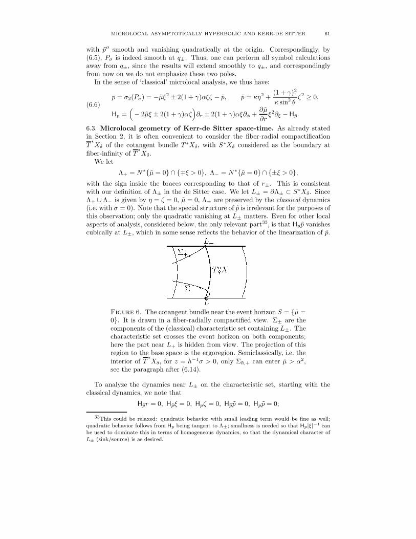
MICROLOCAL ASYMPTOTICALLY HYPERBOLIC AND KERR-DE SITTER 61
with p′′ smooth and vanishing quadratically at the origin. Correspondingly, by(6.5), Pσ is indeed smooth at q±. Thus, one can perform all symbol calculationsaway from q±, since the results will extend smoothly to q±, and correspondinglyfrom now on we do not emphasize these two poles.
In the sense of ‘classical’ microlocal analysis, we thus have:
p = σ2(Pσ) = −µξ2 ± 2(1 + γ)αξζ − p, p = κη2 +(1 + γ)2
κ sin2 θζ2 ≥ 0,
Hp =(− 2µξ ± 2(1 + γ)αζ
)∂r ± 2(1 + γ)αξ∂φ +
∂µ
∂rξ2∂ξ − Hp.
(6.6)
6.3. Microlocal geometry of Kerr-de Sitter space-time. As already statedin Section 2, it is often convenient to consider the fiber-radial compactification
T∗Xδ of the cotangent bundle T ∗Xδ, with S∗Xδ considered as the boundary at
fiber-infinity of T∗Xδ.
We let
Λ+ = N∗µ = 0 ∩ ∓ξ > 0, Λ− = N∗µ = 0 ∩ ±ξ > 0,with the sign inside the braces corresponding to that of r±. This is consistentwith our definition of Λ± in the de Sitter case. We let L± = ∂Λ± ⊂ S∗Xδ. SinceΛ+ ∪ Λ− is given by η = ζ = 0, µ = 0, Λ± are preserved by the classical dynamics(i.e. with σ = 0). Note that the special structure of p is irrelevant for the purposes ofthis observation; only the quadratic vanishing at L± matters. Even for other localaspects of analysis, considered below, the only relevant part33, is that Hpp vanishescubically at L±, which in some sense reflects the behavior of the linearization of p.
Figure 6. The cotangent bundle near the event horizon S = µ =0. It is drawn in a fiber-radially compactified view. Σ± are thecomponents of the (classical) characteristic set containing L±. Thecharacteristic set crosses the event horizon on both components;here the part near L+ is hidden from view. The projection of thisregion to the base space is the ergoregion. Semiclassically, i.e. the
interior of T∗Xδ, for z = h−1σ > 0, only Σ~,+ can enter µ > α2,
see the paragraph after (6.14).
To analyze the dynamics near L± on the characteristic set, starting with theclassical dynamics, we note that
Hpr = 0, Hpξ = 0, Hpζ = 0, Hpp = 0, Hpp = 0;
33This could be relaxed: quadratic behavior with small leading term would be fine as well;quadratic behavior follows from Hp being tangent to Λ±; smallness is needed so that Hp|ξ|−1 canbe used to dominate this in terms of homogeneous dynamics, so that the dynamical character ofL± (sink/source) is as desired.
62 ANDRAS VASY
note that Hpp = 0 and Hpζ = 0 correspond to the integrability of the Hamiltoniandynamical system; these were observed by Carter [6] in the Kerr setting. Further-more,
(6.7) Hp|ξ|−1|S∗Xδ= −(sgn ξ)
∂µ
∂r,
so at ∂N∗µ = 0 it is given by ±(sgn ξ)z±, which is bounded away from 0. Wenote that
(6.8) |ξ|−1Hp(|ξ|−2p)|S∗Xδ
= −2(sgn ξ)∂µ
∂rp|ξ|−2.
Since p = 0 and µ 6= 0 implies ξ = 0 on the classical characteristic set (i.e. when wetake σ = 0), which cannot happen on S∗X (we are away from the zero section!), thisshows that the Hamilton vector field is non-radial except possibly at Λ±. Moreover,
Hp
(µ ∓ 2(1 + γ)α
ζ
ξ
)|S∗Xδ
= −2|ξ|(
µ ∓ 2(1 + γ)αζ
ξ
)(sgn ξ)
∂µ
∂r;
as usual, this corresponds to p = |ξ|−2p at L±. Finally, the imaginary part of thesubprincipal symbol at L± is
((sgn ξ)∂µ
∂r)(β± Im σ)|ξ|, where
β± = ∓2
(dµ
dr
)−1
(1 + γ)(r2 + α2)|r=r± = 2z−1± (1 + γ)(r2
± + α2) > 0;
(6.9)
here (sgn ξ)∂µ∂r was factored out in view of (6.7), (2.5) and (2.3).
Thus, L+ is a sink, L− a source. Furthermore, in the classical sense, ξ = 0 isdisjoint from the characteristic set in the region of validity of the form (6.5) of theoperator, as well as at the poles of the sphere (i.e. the only issue is when r is fartherfrom r±), so the characteristic set has two components there with L± lying indifferent components. We note that that as γ < 1, κ sin2 θ = sin2 θ(1+ γ)− γ sin4 θhas its maximum at θ = π/2, where it is 1. Since on the characteristic set
(6.10) α2ξ2 + (1 + γ)2ζ2 ≥ ±2(1 + γ)αξζ = p + µξ2 ≥ η2 + (1 + γ)2ζ2 + µξ2
and ξ 6= 0, we conclude that
(6.11) µ ≤ α2
there, so this form of the operator remains valid, and the characteristic set canindeed be divided into two components, separating L±.
Next, we note that if α is so large that at r = r0 with dµdr (r0) = 0, one has
µ(r0) = α2, then letting η0 = 0, θ0 = π2 , ξ0 6= 0, ζ0 = ± α
1+γ ξ0, the bicharacteristics
through (r0, θ0, φ0, ξ0, η0, ζ0) are stationary for any φ0, so the operator is classicallytrapping in the strong sense that not only is the Hamilton vector field radial, but itvanishes. Since such vanishing means that weights cannot give positivity in positivecommutator estimates, see Section 2, it is natural to impose the restriction on αthat
(6.12) r0 ∈ (r+, r−),dµ
dr(r0) = 0 ⇒ α2 < µ(r0).
Under this assumption, by (6.11), the ergoregions from the two ends do not inter-sect.
MICROLOCAL ASYMPTOTICALLY HYPERBOLIC AND KERR-DE SITTER 63
Finally, we show that bicharacteristics leave the region µ > µ0, where µ0 < 0is such that dµ
dr is bounded away from 0 on [µ0, (1 + ε)α2]µ for some ε > 0, whichcompletes checking the hypotheses in the classical sense. Note that by (6.2) and(6.12) such µ0 and ε exists. To see this, we use p to measure the size of thecharacteristic set over points in the base. Using ab ≤ (1 + ε)a2 + b2/(1 + ε) andκ sin2 θ ≤ 1, we note that on the characteristic set
(1 + ε)α2ξ2 +(1 + γ)2
1 + εζ2 ≥ p + µξ2 ≥ ε
1 + εp +
(1 + γ)2
1 + εζ2 + µξ2,
so((1 + ε)α2 − µ) ≥ ε
1 + ε|ξ|−2p,
where now both sides are homogeneous of degree zero, or equivalently functions onS∗Xδ . Note that p = 0 implies that ξ 6= 0 on S∗Xδ , so our formulae make sense. By(6.8), using that ∂µ
∂r is bounded away from 0, |ξ|−2p is growing exponentially in theforward/backward direction along the flow as long as the flow remains in a regionµ ≥ µ0, where the form of the operator is valid (which is automatic in this region,as farther on ‘our side’ of the event horizon, X+, where the form of the operatoris not valid, it is elliptic), which shows that the bicharacteristics have to leave thisregion. As noted already, this proves that the operator fits into our framework inthe classical sense.
6.4. Semiclassical behavior. The semiclassical principal symbol is
p~,z = − µ(ξ ± cz
)2 ∓ 2(1 + γ)(r2 + α2)(ξ ± cz
)z ± 2(1 + γ)α
(ξ ± cz
)ζ − p~,z
(6.13)
with
p~,z = κη2 +(1 + γ)2
κ sin2 θ(−α sin2 θz + ζ)2.
Recall now that Mδ = Xδ× [0,∞)τ , and that, due to Section 3.2, we need to choosec in our definition of τ so that dτ
τ is time-like with respect to G. But
〈dτ
τ,dτ
τ〉G = −µc2 − 2c(1 + γ)(r2 + α2) − α2(1 + γ)2 sin2 θ
κ,
and as this must be positive for all θ, we need to arrange that
(6.14) µc2 + 2c(1 + γ)(r2 + α2) + α2(1 + γ)2 < 0,
and this in turn suffices. Note that c = −µ−1(1+γ)(r2 +α2) automatically satisfiesthis in µ > 0; this would correspond to undoing our change of coordinates in (6.4)(which is harmless away from µ = 0, but of course c needs to be smooth at µ = 0).At µ = 0, (6.14) gives a (negative) upper bound for c; for µ > 0 we have an intervalof possible values of c; for µ < 0 large negative values of c always work. Thus,we may choose a smooth function c such that (6.14) is satisfied everywhere, andwe may further arrange that c = −µ−1(1 + γ)(r2 + α2) for µ > µ1 where µ1 is anarbitrary positive constant; in this case, as already discussed, p~,z is semiclassicallyelliptic when Im z 6= 0.
Note also that, as discussed in Subsection 3.2, there is only one component ofthe characteristic set in µ > α2 by (6.11), namely Σ~,sgn(Re z).
It remains to discuss trapping. Note that the dynamics depends continuously onα, with α = 0 being the de Sitter-Schwarzschild case, when there is no trapping nearthe event horizon, so the same holds for Kerr-de Sitter with slow rotation. Below we
64 ANDRAS VASY
first describe the dynamics in de Sitter-Schwarzschild space explicitly, and then, in(6.22), give an explicit range of α in which the non-trapping dynamical assumption,apart from hyperbolic trapping, is satisfied.
First, on de Sitter-Schwarzschild space, recalling that c is irrelevant for the dy-namics for real z, we may take c = 0 (i.e. otherwise we would simply change thiscalculation by the effect of a symplectomorphism, corresponding to a conjugation,which we note does not affect the ‘base’ variables on the cotangent bundle). Then
p~,z = −µξ2 ∓ 2r2ξz − p~,z, p~,z = η2 +ζ2
sin2 θ,
so
Hp~,z= −2(µξ ± r2z)∂r +
(∂µ
∂rξ2 ± 4rzξ
)∂ξ − Hp~,z
,
hence Hp~,zr = −2(µξ ± r2z), and so Hp~,z
r = 0 implies ∓z = r−2µξ. We first notethat Hp~,z
r cannot vanish in T ∗Xδ in µ ≤ 0 (though it can vanish at fiber infinityat L±) since (for z 6= 0)
(6.15) µ ≤ 0 and Hp~,zr = 0 ⇒ µξ 6= 0 and p~,z = µξ2 − p~,z < 0.
It remains to consider Hp~,zr = 0 in µ > 0. At such a point
H2p~,z
r = −2µHp~,zξ = −2µξ2
(∂µ
∂r− 4r−1µ
)= −2µξ2r4 ∂(r−4µ)
∂r,
so as ∓z = r−2µξ, so ξ 6= 0, by the discussion after (6.2),
µ > 0, ±(r − 3
2rs) > 0, Hp~,z
r = 0 ⇒ ±H2p~,z
r > 0,
and thus the gluing hypotheses of [13] are satisfied arbitrarily close to34 r = 32rs.
Furthermore, as p~,z = −µ−1(µξ ± r2z)2 + r4z2 − p~,z, if r = 32rs, Hp~,z
r = 0 and
p~,z = 0 then p~,z = r4z2, so with
Γz = r =3
2rs, µξ ± r2z = 0, p~,z = r4z2,
we have
(6.16) p~,z($) = 0, µ($) > 0, $ /∈ Γz, (Hp~,zr)($) = 0 ⇒ (±H
2p~,z
r)($) > 0,
with ± corresponding to whether r > 32rs or r < 3
2rs. In particular, taking intoaccount (6.15), r gives rise to an escape function in T ∗Xδ \ Γz as discussed inFootnote 16, and Γz is the only possible trapping. (In this statement we ignorefiber infinity.) Correspondingly, if one regards a compact interval I in (r−, 3
2rs), or
( 32rs, r+) as the gluing region, for sufficiently small α, for r ∈ I , Hp~,z
r = 0 still
implies ±H2p~,z
r > 0, and [13] is applicable. If instead one works with compact
subsets of µ > 0 \ Γz, one has non-trapping dynamics for α small.Since in [52, Section 2] Wunsch and Zworski only check normal hyperbolicity in
Kerr space-times with sufficiently small angular momentum, in order to use theirgeneral results for normally hyperbolic trapped sets, we need to check that Kerr-deSitter space-times are still normally hyperbolic. For this, with small α, we follow
34Or far from, in µ > 0.
MICROLOCAL ASYMPTOTICALLY HYPERBOLIC AND KERR-DE SITTER 65
[52, Section 2], and note that for α = 0 the linearization of the flow at Γ in thenormal variables r − 3
2rs and µξ ± r2z is
[r − 3
2rs
µξ ± r2z
]′=
[0 −2( 3
2rs)4z2µ|−1
r= 32rs
−2 0
] [r − 3
2rs
µξ ± r2z
]+O((r− 3
2rs)
2 +(µξ±r2z)2),
so the eigenvalues of the linearization are λ = ±3√
3rsz(1− 9
4Λr2s
)−1/2, in agreement
with the result of [52] when Λ = 0. The rest of the arguments concerning the flowin [52, Section 2] go through. In particular, when analyzing the flow within Γ =∪z>0Γz, the pull backs of both dp and dζ are exactly as in the Schwarzschild setting(unlike the normal dynamics, which has different eigenvalues), so the arguments of[52, Proof of Proposition 2.1] go through unchanged, giving normal hyperbolicityfor small α by the structural stability.
We now check the hyperbolic nature of trapping for larger values of α. Withc = 0, as above,
p~,z = −µξ2 ∓ 2(1 + γ)((r2 + α2)z − αζ
)ξ − p~.z,
and in the region µ > 0 this can be rewritten as
p~,z = −µ
(ξ ± 1 + γ
µ
((r2 + α2)z − αζ
))2
+(1 + γ)2
µ
((r2 + α2)z − αζ
)2 − p~.z;
note that the first term would be just −µξ2 in the original coordinates (6.1) whichare valid in µ > 0. Thus,
(6.17) Hp~.zr = −2
(µξ ± (1 + γ)
((r2 + α2)z − αζ
)).
Correspondingly,
µ ≤ 0, Hp,~,zr = 0 ⇒ p~,z = µξ2 − p~.z ≤ 0,
and equality on the right hand side implies ζ = α sin2 θz, so Hp~,zr = (r2 +
α2 cos2 θ)z > 0, a contradiction, showing that in µ ≤ 0, Hp~,zr cannot vanish
on the characteristic set.We now turn to µ > 0, where
Hp~,zr = 0 ⇒ H
2p~,z
r = −2µHp~,zξ = 2µ(1 + γ)2
∂
∂r
(µ−1
((r2 + α2)z − αζ
)2).
Thus, we are interested in critical points of
F = µ−1((r2 + α2)z − αζ
)2,
and whether these are non-degenerate. We remark that
Hp~,zr = 0 and (r2 + α2)z − αζ = 0 and p~,z = 0 ⇒ ξ = 0 and p~,z = 0;
p~,z = 0 and (r2 + α2)z − αζ = 0 and p~,z = 0 ⇒ (r2 + α2 cos2 θ)z = 0;
which is a contradiction, so (r2 + α2)z − αζ does not vanish when p~,z and Hp~,zr
do. Note that
(6.18)∂F
∂r= −
((r2 + α2)z − αζ
)µ−2f, f =
((r2 + α2)z − αζ
)∂µ
∂r− 4rµz,
so
(6.19)∂F
∂r= 0 and (r2 + α2)z − αζ 6= 0 ⇒ ∂2F
∂r2= −
((r2 + α2)z − αζ
)µ−2 ∂f
∂r.
66 ANDRAS VASY
Also, from (6.18),
µ > 0, f = 0 ⇒ ∂µ
∂r6= 0.
Now
(6.20)∂f
∂r=((r2 + α2)z − αζ
)∂2µ
∂r2− 4µz − 2rz
∂µ
∂r,
and∂F
∂r= 0 ⇒ (r2 + α2)z − αζ =
4rµz∂µ∂r
,
so substituting into (6.20),
(6.21)∂µ
∂r
∂f
∂r= 4rµz
∂2µ
∂r2− 4zµ
∂µ
∂r− 2rz
(∂µ
∂r
)2
.
Thus,
∂µ
∂r
∂f
∂r= 2z
(2µ
(r∂2µ
∂r2− 3
∂µ
∂r
)− (r
∂µ
∂r− 4µ)
∂µ
∂r
),
so taking into account
r∂µ
∂r− 4µ = −2
(1 − Λα2
3
)r2 + 3rsr − 4α2,
r∂2µ
∂r2− 3
∂µ
∂r= −4
(1 − Λα2
3
)r + 3rs,
r∂2µ
∂r2− 3
∂µ
∂r=
2
r
(r∂µ
∂r− 4µ
)− 3rs +
8α2
r,
we obtain
∂µ
∂r
∂f
∂r= 2z
(−1
r
(r∂µ
∂r− 4µ
)2
− 2µ
r(3rsr − 8α2)
).
We claim that if |α| < rs/2 then r− > rs/2. To see this, note that for r = rs/2,
µ(r) =
(r2s
4+ α2
)(1 − Λr2
s
12
)− r2
s
2< 0;
since at α = 0, r− > rs/2, we deduce that r− > rs/2 for |α| < rs/2. Making theslightly stronger assumption,
(6.22) |α| <
√3
4rs,
we obtain that for µ > 0, r > r−, 3rsr − 8α2 > 32r2
s − 8α2 > 0, so
z∂µ
∂r
∂f
∂r< 0.
Thus, when ∂F∂r = 0, using (6.19),
(6.23)∂2F
∂r2= −
((r2 + α2)z − αζ
)µ−2 ∂f
∂r= − 4r
µ(
∂µ∂r
)2 z∂µ
∂r
∂f
∂r> 0,
so critical points of F are all non-degenerate and are minima. Correspondingly,as F → +∞ as µ → 0 in µ > 0, the critical point rc of F exists and is unique
MICROLOCAL ASYMPTOTICALLY HYPERBOLIC AND KERR-DE SITTER 67
in (r−, r+) (when ζ is fixed), depends smoothly on ζ, and ∂F∂r > 0 if r > rc, and
∂F∂r < 0 if r < rc. Thus,
µ > 0, ±(r − rc) > 0, Hp~,zr = 0 ⇒ ±H
2p~,z
r > 0,
giving the natural generalization of (6.16), allowing the application of the resultsof [13]. Since Hp~,z
r cannot vanish in µ ≤ 0 (apart from fiber infinity, which isunderstood already), we conclude that r gives rise to an escape function, as inFootnote 16, away from
Γz = $ :∂F
∂r($) = 0, (Hp~,z
r)($) = 0, p~,z($) = 0,
which is a smooth submanifold as the differentials of the defining functions arelinearly independent on it in view of (6.23), (6.17), and the definition of p~,z (asthe latter is independent of r and ξ).
The linearization of the Hamilton flow at Γz is[
r − rc
µξ ± (1 + γ)((r2 + α2)z − αζ
)]′
=
[0 −µ(1 + γ)2 ∂2F
∂r2
−2 0
] [r − rc
µξ ± (1 + γ)((r2 + α2)z − αζ
)]
+ O((r − rc)
2 +(µξ ± (1 + γ)
((r2 + α2)z − αζ
))2),
so by (6.23), the linearization is non-degenerate, and is indeed hyperbolic. Thissuffices for the resolvent estimates of [52] for exact Kerr-de Sitter, but for stabilityone also needs to check normal hyperbolicity. While it is quite straightforward tocheck that the only degenerate location is η = 0, θ = π
2 , the computation of theMorse-Bott non-degeneracy in the spirit of [52, Proof of Proposition 2.1], where itis done for Kerr spaces with small angular momentum, is rather involved, so we donot pursue this here (for small angular momentum in Kerr-de Sitter space, the deSitter-Schwarzschild calculation above implies normal hyperbolicity already).
In addition, in view of an overall sign difference between our convention and thatof [52] for the operator we are considering, [52] requires the positivity of z ∂
∂z p~,z forz 6= 0. (Note that the notation for z is also different; our z is 1 + z in the notationof [52], so our z being near 1 corresponds to the z of [52] being near 0.) Unlikethe flow, whose behavior is independent of c when z is real, this fact does dependon the choice of c. Note that in the high energy version, this corresponds to thepositivity of σ ∂
∂σ pfull. Now, pfull = 〈σ dττ +$, σ dτ
τ +$〉G, with $ ∈ Π, the ‘spatial’
hyperplane, identified with T ∗X in bT ∗M , so
σ∂σpfull = 2〈σ dτ
τ, σ
dτ
τ〉G + 2〈σ dτ
τ, $〉G
= σ2〈dτ
τ,dτ
τ〉G + 〈σ dτ
τ+ $, σ
dτ
τ+ $〉G − 〈$, $〉G.
Thus, if non-zero elements of Π are space-like and dττ is time-like, σ∂σpfull > 0 for
σ 6= 0 on the characteristic set of pfull. If c is such that c = −µ−1(1 + γ)(r2 + α2)near r = 3
2rs, which as we mentioned can be arranged, and which corresponds toundoing our change of coordinates in (6.4), then directly from (6.1) both the time-like and space-like statements hold, completing our checking of the hypotheses of[52], and thus their result is applicable for de Sitter-Schwarzschild space-times. As
68 ANDRAS VASY
these results are structurally stable, see the proof of [52, Proposition 2.1], the resultfollows for Kerr-de Sitter spaces with angular momenta satisfying (6.22).
6.5. Complex absorption. The final step of fitting Pσ into a general microlocalframework is moving the problem to a compact manifold, and adding a complexabsorbing second order operator. This section is almost completely parallel to Sub-section 4.7 in the de Sitter case; the only change is that absorption needs to beadded at the trapped set as well.
We thus consider a compact manifold without boundary X for which Xδ isidentified as an open subset with smooth boundary; we can again take X to be thedouble of Xδ. As in the de Sitter case, we discuss the ‘classical’ and ‘semiclassical’cases separately, for in the former setting trapping does not matter, while in thelatter it does.
We then introduce a complex absorbing operator Qσ ∈ Ψ2cl(X) with principal
symbol q, such that h2Qh−1z ∈ Ψ2~,cl(X) with semiclassical principal symbol q~,z,
and such that p ± ıq is elliptic near ∂Xδ, i.e. near µ = µ0, and which satisfies thatthe ±q ≥ 0 on Σ∓. Having done this, we extend Pσ and Qσ to X in such a waythat p ± ıq are elliptic near X \ Xδ; the region we added is thus irrelevant. Inparticular, as the event horizon is characteristic for the wave equation, the solutionin the exterior of the event horizons is unaffected by thus modifying Pσ , i.e. workingwith Pσ and Pσ − ıQσ is equivalent for this purpose.
Again, as in de Sitter space, an alternative to this extension would be simplyadding a boundary at µ = µ0; this is easy to do since this is a space-like hypersur-face, see Remark 2.5.
For the semiclassical problem, when z is almost real we need to increase the re-quirements on Qσ. We need in addition, in the semiclassical notation, semiclassicalellipticity near µ = µ0, i.e. that p~,z ± ıq~,z are elliptic near ∂Xδ, i.e. near µ = µ0,and which satisfies that ±q~,z ≥ 0 on Σ~,∓. However, we also need semiclassicalellipticity at the trapped set, which is in X+. To achieve this, we want q~,z ellipticon the trapped set; since this is in Σ~,sgnRe z, we need q~,z ≤ 0 there. Again, weextend Pσ and Qσ to X in such a way that p ± ıq and p~,z ± ıq~,z are elliptic nearX \ Xδ; the region we added is thus irrelevant. For α as in (6.22), the dynamics(away from the radial points) has only the hyperbolic trapping (and for small α, itis normally hyperbolic); however, our results apply more generally, as long as thedynamics has the same non-trapping character (so α might be even larger). Notealso that since the trapping is in a compact subset of X+ = µ > 0, one canarrange that Qσ is the sum of two terms: one supported near the trapping in X+,the other in µ < 0; this is useful for relating our construction to that of Dyatlov[18] in the appendix.
This completes the setup. Now all of the results of Section 2 are applicable,proving all the theorems stated in the introduction on Kerr-de Sitter spaces, The-orems 1.1-1.4. Namely, Theorem 1.1 follows from Theorem 2.13, Theorem 1.2follows from Theorem 2.10, Theorem 1.3 follows from Theorem 2.17. Finally The-orem 1.4 is an immediate consequence of Theorem 1.3 and the Mellin transformlemma, Lemma 3.1, in the Kerr-de Sitter setting, or Proposition 3.3 for general b-perturbations (so ∂t may no longer be Killing, and the space-time may no longer bestationary), either taking into account that by usual energy estimates the complexabsorbing region cannot affect the solution in a neighborhood of X+, or simply, for
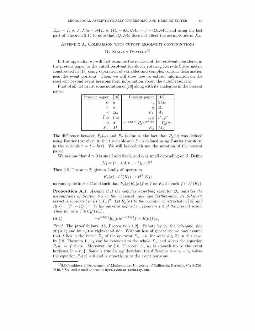
MICROLOCAL ASYMPTOTICALLY HYPERBOLIC AND KERR-DE SITTER 69
gu = f , so PσMu = Mf , so (Pσ − ıQσ)Mu = f − ıQσMu, and using the lastpart of Theorem 2.15 to note that ıQσMu does not affect the asymptotics in Xδ .
Appendix A. Comparison with cutoff resolvent constructions
By Semyon Dyatlov35
In this appendix, we will first examine the relation of the resolvent considered inthe present paper to the cutoff resolvent for slowly rotating Kerr–de Sitter metricconstructed in [18] using separation of variables and complex contour deformationnear the event horizons. Then, we will show how to extract information on theresolvent beyond event horizons from information about the cutoff resolvent.
First of all, let us list some notation of [18] along with its analogues in the presentpaper:
Present paper [18] Present paper [18]α a rs 2M0
γ α µ ∆r
κ ∆θ F± A±
t, φ t, ϕ t, φ t∗, ϕ∗
ω σ e−iσh(r)Pσeiσh(r) −Pg(σ)X+ M Kδ MK
The difference between Pg(ω) and Pσ is due to the fact that Pg(ω) was definedusing Fourier transform in the t variable and Pσ is defined using Fourier transformin the variable t = t + h(r). We will henceforth use the notation of the presentpaper.
We assume that δ > 0 is small and fixed, and α is small depending on δ. Define
Kδ = (r− + δ, r+ − δ)r × S2.
Then [18, Theorem 2] gives a family of operators
Rg(σ) : L2(Kδ) → H2(Kδ)
meromorphic in σ ∈ C and such that Pg(σ)Rg(σ)f = f on Kδ for each f ∈ L2(Kδ).
Proposition A.1. Assume that the complex absorbing operator Qσ satisfies theassumptions of Section 6.5 in the ‘classical’ case and furthermore, its Schwartzkernel is supported in (X \X+)2. Let Rg(σ) be the operator constructed in [18] andR(σ) = (Pσ − iQσ)−1 be the operator defined in Theorem 1.2 of the present paper.Then for each f ∈ C∞
0 (Kδ),
(A.1) −eiσh(r)Rg(σ)e−iσh(r)f = R(σ)f |Kδ.
Proof. The proof follows [18, Proposition 1.2]. Denote by u1 the left-hand sideof (A.1) and by u2 the right-hand side. Without loss of generality, we may assumethat f lies in the kernel D′
k of the operator Dφ − k, for some k ∈ Z; in this case,by [18, Theorem 1], u1 can be extended to the whole X+ and solves the equationPσu1 = f there. Moreover, by [18, Theorem 3], u1 is smooth up to the eventhorizons r = r±. Same is true for u2; therefore, the difference u = u1 − u2 solvesthe equation Pσ(u) = 0 and is smooth up to the event horizons.
35S.D.’s address is Department of Mathematics, University of California, Berkeley, CA 94720-3840, USA, and e-mail address is [email protected].
70 ANDRAS VASY
Since both sides of (A.1) are meromorphic, we may further assume that Im σ >Ce, where Ce is a large constant. Now, the function u(t, ·) = e−itσu(·) solves thewave equation gu = 0 and is smooth up to the event horizons in the coordinatesystem (t, r, θ, φ); therefore, if Ce is large enough, by [18, Proposition 1.1] u cannotgrow faster than exp(Cet). Therefore, u = 0 as required.
Now, we show how to express the resolvent R(σ) on the whole space in termsof the cutoff resolvent Rg(σ) and the nontrapping parametrix constructed in thepresent paper. Let Qσ be as above, but with the additional assumption of semi-classical ellipticity near ∂Xδ, and Q′
σ be an operator satisfying the assumptionsof Section 6.5 in the ‘semiclassical’ case on the trapped set. Moreover, we requirethat the semiclassical wavefront set of |σ|−2Q′
σ be compact and Q′σ = χQ′
σ = Q′σχ,
where χ ∈ C∞0 (Kδ). Such operators exist for α small enough, as the trapped set is
compact and located O(α) close to the photon sphere r = 3rs/2 and thus is farfrom the event horizons. Denote R′(σ) = (Pσ − iQσ − iQ′
σ)−1; by Theorem 2.13applied in the case of Section 6.5, for each C0 there exists a constant σ0 such thatfor s large enough, Im σ > −C0, and |Re σ| > σ0,
‖R′(σ)‖Hs−1
|σ|−1→Hs
|σ|−1≤ C|σ|−1.
We now use the identity
(A.2) R(σ) = R′(σ) − R′(σ)(iQ′σ + Q′
σ(χR(σ)χ)Q′σ)R′(σ).
(To verify it, multiply both sides of the equation by Pσ − iQσ − iQ′σ on the left
and on the right.) Combining (A.2) with the fact that for each N , Q′σ is bounded
H−N|σ|−1 → HN
|σ|−1 with norm O(|σ|2), we get for σ not a pole of χR(σ)χ,
(A.3) ‖R(σ)‖Hs−1
|σ|−1→Hs
|σ|−1≤ C(1 + |σ|2‖χR(σ)χ‖L2(Kδ)→L2(Kδ)).
Also, if σ0 is a pole of R(σ) of algebraic multiplicity j, then we can multiply theidentity (A.2) by (σ − σ0)
j to get an estimate similar to (A.3) on the function(σ − σ0)
jR(σ), holomorphic at σ = σ0.The discussion above in particular implies that the cutoff resolvent estimates
of [5] also hold for the resolvent R(σ). Using the Mellin transform, we see that theresonance expansion of [5] is valid for any solution u to the forward time Cauchyproblem for the wave equation on the whole Mδ, with initial data in a high enoughSobolev class; the terms of the expansion are defined and the remainder is estimatedon the whole Mδ as well.
References
[1] D. Baskin. A parametrix for the fundamental solution of the Klein-Gordon equation onasymptotically de Sitter spaces. Preprint, arxiv:0905.0447, 2009.
[2] Lydia Bieri. Part I: Solutions of the Einstein vacuum equations. In Extensions of the stabilitytheorem of the Minkowski space in general relativity, volume 45 of AMS/IP Stud. Adv. Math.,pages 1–295. Amer. Math. Soc., Providence, RI, 2009.
[3] Lydia Bieri and Nina Zipser. Extensions of the stability theorem of the Minkowski spacein general relativity, volume 45 of AMS/IP Studies in Advanced Mathematics. AmericanMathematical Society, Providence, RI, 2009.
[4] P. Blue and A. Soffer. Phase space analysis on some black hole manifolds. J. Funct. Anal.,
256(1):1–90, 2009.[5] Jean-Francois Bony and Dietrich Hafner. Decay and non-decay of the local energy for the
wave equation on the de Sitter-Schwarzschild metric. Comm. Math. Phys., 282(3):697–719,2008.
MICROLOCAL ASYMPTOTICALLY HYPERBOLIC AND KERR-DE SITTER 71
[6] B. Carter. Global structure of the kerr family of gravitational fields. Phys. Rev., 174:1559–1571, 1968.
[7] Demetrios Christodoulou and Sergiu Klainerman. The global nonlinear stability of theMinkowski space, volume 41 of Princeton Mathematical Series. Princeton University Press,Princeton, NJ, 1993.
[8] Mihalis Dafermos and Igor Rodnianski. A proof of Price’s law for the collapse of a self-gravitating scalar field. Invent. Math., 162(2):381–457, 2005.
[9] Mihalis Dafermos and Igor Rodnianski. The wave equation on Schwarzschild-de Sitter spacetimes. Preprint, arXiv:07092766, 2007.
[10] Mihalis Dafermos and Igor Rodnianski. The red-shift effect and radiation decay on black holespacetimes. Comm. Pure Appl. Math, 62:859–919, 2009.
[11] Mihalis Dafermos and Igor Rodnianski. The black hole stability problem for linear scalarperturbations. Preprint, arXiv:1010.5137, 2010.
[12] Mihalis Dafermos and Igor Rodnianski. Decay of solutions of the wave equation on Kerrexterior space-times I-II: The cases of |a| m or axisymmetry. Preprint, arXiv:1010.5132,2010.
[13] K. Datchev and A. Vasy. Gluing semiclassical resolvent estimates via propagation of singu-larities. Preprint, arxiv:1008.3064, 2010.
[14] K. Datchev and A. Vasy. Propagation through trapped sets and semiclassical resolvent esti-
mates. Preprint, arxiv:1010.2190, 2010.[15] Mouez Dimassi and Johannes Sjostrand. Spectral asymptotics in the semi-classical limit,
volume 268 of London Mathematical Society Lecture Note Series. Cambridge University Press,Cambridge, 1999.
[16] R. Donninger, W. Schlag, and A. Soffer. A proof of price’s law on schwarzschild black holemanifolds for all angular momenta. Preprint, arxiv:0908.4292, 2009.
[17] Semyon Dyatlov. Exponential energy decay for Kerr-de Sitter black holes beyond event hori-zons. Preprint, arxiv:1010.5201, 2010.
[18] Semyon Dyatlov. Quasi-normal modes and exponential energy decay for the Kerr-de Sitterblack hole. Preprint, arxiv:1003.6128, 2010.
[19] Lawrence C. Evans and Maciej Zworski. Lectures on semiclassical analysis. Preprint, 2010.[20] Charles Fefferman and C. Robin Graham. Conformal invariants. Asterisque, (Numero Hors
Serie):95–116, 1985. The mathematical heritage of Elie Cartan (Lyon, 1984).[21] F. Finster, N. Kamran, J. Smoller, and S.-T. Yau. Decay of solutions of the wave equation
in the Kerr geometry. Comm. Math. Phys., 264(2):465–503, 2006.[22] Felix Finster, Niky Kamran, Joel Smoller, and Shing-Tung Yau. Linear waves in the Kerr
geometry: a mathematical voyage to black hole physics. Bull. Amer. Math. Soc. (N.S.),46(4):635–659, 2009.
[23] F. G. Friedlander. Radiation fields and hyperbolic scattering theory. Math. Proc. CambridgePhilos. Soc., 88(3):483–515, 1980.
[24] C. Guillarmou, A. Hassell, and A. Sikora. Resolvent at low energy III: The spectral measure.Preprint, arxiv:1009.3084, 2010.
[25] Colin Guillarmou. Meromorphic properties of the resolvent on asymptotically hyperbolicmanifolds. Duke Math. J., 129(1):1–37, 2005.
[26] A. Hassell, R. B. Melrose, and A. Vasy. Spectral and scattering theory for symbolic potentialsof order zero. Advances in Mathematics, 181:1–87, 2004.
[27] A. Hassell, R. B. Melrose, and A. Vasy. Microlocal propagation near radial points and scat-tering for symbolic potentials of order zero. Analysis and PDE, 1:127–196, 2008.
[28] L. Hormander. The analysis of linear partial differential operators, vol. 1-4. Springer-Verlag,1983.
[29] Bernard S. Kay and Robert M. Wald. Linear stability of Schwarzschild under perturbationswhich are nonvanishing on the bifurcation 2-sphere. Classical Quantum Gravity, 4(4):893–898, 1987.
[30] Hans Lindblad and Igor Rodnianski. Global existence for the Einstein vacuum equations inwave coordinates. Comm. Math. Phys., 256(1):43–110, 2005.
[31] Hans Lindblad and Igor Rodnianski. The global stability of Minkowski space-time in harmonicgauge. Ann. of Math. (2), 171(3):1401–1477, 2010.
[32] Jeremy Marzuola, Jason Metcalfe, Daniel Tataru, and Mihai Tohaneanu. Strichartz estimateson Schwarzschild black hole backgrounds. Comm. Math. Phys., 293(1):37–83, 2010.
72 ANDRAS VASY
[33] R. Mazzeo and R. B. Melrose. Meromorphic extension of the resolvent on complete spaceswith asymptotically constant negative curvature. J. Func. Anal., 75:260–310, 1987.
[34] Rafe Mazzeo. Elliptic theory of differential edge operators. I. Comm. Partial DifferentialEquations, 16(10):1615–1664, 1991.
[35] R. B. Melrose. Spectral and scattering theory for the Laplacian on asymptotically Euclidianspaces. Marcel Dekker, 1994.
[36] R. B. Melrose, A. Sa Barreto, and A. Vasy. Asymptotics of solutions of the wave equation onde Sitter-Schwarzschild space. Preprint, arxiv:0811.2229, 2008.
[37] R. B. Melrose, A. Sa Barreto, and A. Vasy. Analytic continuation and semiclassical resolventestimates on asymptotically hyperbolic spaces. Work in progress, 2010.
[38] R. B. Melrose, A. Vasy, and J. Wunsch. Diffraction of singularities for the wave equation onmanifolds with corners. arXiv:0903.3208, 2009.
[39] Richard B. Melrose. The Atiyah-Patodi-Singer index theorem, volume 4 of Research Notesin Mathematics. A K Peters Ltd., Wellesley, MA, 1993.
[40] Stephane Nonnenmacher and Maciej Zworski. Quantum decay rates in chaotic scattering.Acta Math., 203(2):149–233, 2009.
[41] D. Polarski. On the Hawking effect in de Sitter space. Classical Quantum Gravity, 6(5):717–722, 1989.
[42] Antonio Sa Barreto and Jared Wunsch. The radiation field is a Fourier integral operator.
Ann. Inst. Fourier (Grenoble), 55(1):213–227, 2005.[43] Antonio Sa Barreto and Maciej Zworski. Distribution of resonances for spherical black holes.
Math. Res. Lett., 4(1):103–121, 1997.[44] M. A. Shubin. Pseudodifferential operators and spectral theory. Springer-Verlag, 1987.[45] Daniel Tataru. Local decay of waves on asymptotically flat stationary spacetimes. Preprint,
arxiv:0910.5290, 2009.[46] Daniel Tataru and Mihai Tohaneanu. Local energy estimate on Kerr black hole backgrounds.
Preprint, arxiv:0810.5766, 2008.[47] A. Vasy. The wave equation on asymptotically Anti-de Sitter spaces. Preprint,
arxiv:math/0911.5440, 2009.[48] A. Vasy. The wave equation on asymptotically de Sitter-like spaces. Adv. in Math., 223:49–97,
2010.[49] A. Vasy and M. Zworski. Semiclassical estimates in asymptotically Euclidean scattering.
Commun. Math. Phys., 212:205–217, 2000.[50] Robert M. Wald. Note on the stability of the Schwarzschild metric. J. Math. Phys.,
20(6):1056–1058, 1979.[51] F. Wang. Radiation field for vacuum Einstein equation. PhD thesis, Massachusetts Institute
of Technology, 2010.[52] J. Wunsch and M. Zworski. Resolvent estimates for normally hyperbolic trapped sets.
Preprint, arXiv:1003.4640, 2010.[53] Karen Yagdjian and Anahit Galstian. Fundamental solutions for the Klein-Gordon equation
in de Sitter spacetime. Comm. Math. Phys., 285(1):293–344, 2009.
Department of Mathematics, Stanford University, CA 94305-2125, USA
E-mail address: [email protected]