HAL Id: hal-03224820https://hal.archives-ouvertes.fr/hal-03224820

Submitted on 12 May 2021

HAL is a multi-disciplinary open accessarchive for the deposit and dissemination of sci-entific research documents, whether they are pub-lished or not. The documents may come fromteaching and research institutions in France orabroad, or from public or private research centers.

L’archive ouverte pluridisciplinaire HAL, estdestinée au dépôt et à la diffusion de documentsscientifiques de niveau recherche, publiés ou non,émanant des établissements d’enseignement et derecherche français ou étrangers, des laboratoirespublics ou privés.

Micron-scale phenomena observed in a turbulentlaser-produced plasma

G. Rigon, B. Albertazzi, T. Pikuz, P. Mabey, V. Bouffetier, N. Ozaki, T.Vinci, F. Barbato, E. Falize, Y. Inubushi, et al.

To cite this version:G. Rigon, B. Albertazzi, T. Pikuz, P. Mabey, V. Bouffetier, et al.. Micron-scale phenomena observedin a turbulent laser-produced plasma. Nature Communications, Nature Publishing Group, 2021, 12(1), �10.1038/s41467-021-22891-w�. �hal-03224820�

Micron-scale phenomena observed in a turbulent laser-produced

plasma

G. Rigona,1 B. Albertazzi,1 T. Pikuz,2, 3 P. Mabey,1 V. Bouffetier,4 N. Ozaki,5, 6

T. Vinci,1 F. Barbato,4 E. Falize,7 Y. Inubushi,8, 9 N. Kamimura,5 K.

Katagiri,5 S. Makarov,3, 10 M.J.-E. Manuel,11 K. Miyanishi,9 S. Pikuz,3, 12

O. Poujade,7, 13 K. Sueda,9 T. Togashi,8, 9 Y. Umeda,5, 14 M. Yabashi,8, 9

T. Yabuuchi,8, 9 G. Gregori,15 R. Kodama,5 A. Casner,4 and M. Koenig1, 5

1LULI, CNRS, CEA, Ecole Polytechnique,

UPMC, Univ Paris 06: Sorbonne Universites,

Institut Polytechnique de Paris, F-91128 Palaiseau cedex, France

2Institute for Open and Transdisciplinary Research Initiative,

Osaka University, Osaka, 565-0871, Japan

3Joint Institute for High Temperature RAS, Moscow, 125412, Russia

4Universite de Bordeaux-CNRS-CEA, CELIA,

UMR 5107, F-33405 Talence, France

5Graduate School of Engineering, Osaka University, Osaka, 565-0871, Japan

6Institute of Laser Engineering, Osaka University, Suita, Osaka 565-0871, Japan

7CEA-DAM, DIF, F-91297 Arpajon, France

8Japan Synchrotron Radiation Research Institute,

1-1-1 Kouto Sayo-cho, Sayo-gun, Hyogo 679-5198, Japan

9RIKEN SPring-8 Center, 1-1-1 Kouto Sayo-cho, Sayo-gun, Hyogo 679-5148, Japan

10Department of Physics of accelerators and radiation medicine,

Faculty of Physics, Lomonosov Moscow State University, Moscow, 119991, Russia

11General Atomics, Inertial Fusion Technologies,

3550 General Atomics Way, San Diego, CA 92121, USA

12National Research Nuclear University ”MEPhi”, Moscow, 115409, RUSSIA

13Universite Paris-Saclay, CEA, LMCE,

F-91680, Bruyeres-le-Chatel, France

14Institute for Planetary Materials, Okayama University, Misasa, Tottori 682-0193, Japan

a gabriel.rigon@ens-lyon.org

1

15Department of Physics, University of Oxford, Oxford, UK

2

ABSTRACT

Turbulence is ubiquitous in the universe and in fluid dynamics. It influences a wide

range of high energy density systems, from inertial confinement fusion to astrophysical-

object evolution. Understanding this phenomenon is crucial, however, due to limitations in

experimental and numerical methods in plasma systems, a complete description of the tur-

bulent spectrum is still lacking. Here, we present the measurement of a turbulent spectrum

down to micron scale in a laser-plasma experiment. We use a experimental platform, which

couples a high power optical laser, an x-ray free-electron laser and a lithium fluoride crystal,

to study the dynamics of a plasma flow with micrometric resolution (∼1 µm) over a large

field of view (>1 mm2). After the evolution of a Rayleigh-Taylor unstable system, we obtain

spectra, which are overall consistent with existing turbulent theory, but present unexpected

features. This work paves the way towards a better understanding of numerous systems, as

it allows the direct comparison of experimental results, theory and numerical simulations.

This is an author format version.

The article is published in Nature Communication 12, 2679 (2021).

DOI: https://doi.org/10.1038/s41467-021-22891-w

Copyright: Creative Commons Attribution 4.0 International License.

INTRODUCTION

Hydrodynamic turbulence occurs in a variety of systems as a direct consequence of the

non-linearity of the fluid equations [1–4]. In high-energy-density physics (HEDP), it perme-

ates every scale from inertial confinement fusion [5–9] to astrophysical-object evolution [10–

12]. This chaotic phenomenon is believed to develop when the viscosity of a flow is negligible,

which is often considered to be the case in plasma physics (especially in HEDP). It leads

to the creation of 3D eddies of decreasing size, which, carry energy in a cascade from the

large scale of injection, to smaller ones, where dissipation occurs. These eddies, whose dis-

tribution becomes isotropic at a small enough spatial scale, lead to a global homogenisation

of the fluid. This mixing phenomenon plays an important role in numerous systems, either

3

in the laboratory or in the Universe. In inertial confinement fusion, it can hinder, or even

prevent, ignition. In astrophysics, turbulence is also believed to strongly influence super-

novae explosions [12] and can be found in their remnants (see figure 1 a), as well as in the

local non-homogeneous aspect of the interstellar medium, thus affecting the star formation

process [13–15] and the propagation of cosmic rays [16, 17]. Although multiple studies have

already been performed, including HEDP [3, 18], our understanding of turbulence, even in

the classical hydrodynamic case, remains incomplete [19].

The study of turbulent plasma flows includes further complexity (magnetic fields, multi-

ples fluids...), which deviates from the standard approach. Thus, the classical energy cascade

and dissipation microscales of the Kolmogorov theory [1] may not be fully applicable when

dealing with plasma [20]. Usually, turbulence theories are investigated through both nu-

merical simulations and experiments, each with their own limitations. Many experiments

studying turbulence in HEDP are restricted to macroscale metrics, such as the interface

mix-width, since diagnostics can not resolve higher order features [21]. This constraint

severely limits the utility of the experimental approach, since the smallest spatial scales are

often non-negligible and a subject of interest in turbulence studies. For these scales, simu-

lations are often required. Yet, controlled and well diagnosed experiments are nevertheless

mandatory to constrain the predictions of different theories and simulations.

Here, we show results from an experiment where a laser-produced Rayleigh-Taylor unsta-

ble plasma flow evolves towards a possibly turbulent state. The main diagnostic, an x-ray

radiography platform, coupling an x-ray free-electron laser (XFEL) and a lithium-fluoride

crystal (LiF) [22, 23], allowed us to take time-resolved images with sub-micron spatial reso-

lution over a large field of view (>1 mm2 corresponding to the XFEL beam size). From the

obtained radiographs, we extract intensity spatial spectra, which can be associated to ve-

locity spectra. These spectra are compared to turbulence theories and unaccounted features

are discussed. To complete this study, we perform matching simulations using the FLASH4

code [24, 25]. They have been used to infer experimentally unmeasured parameters such as

the pressure or fluid velocity, necessary for our analysis.

4

RESULTS

Experimental setup and diagnostics

The experiment was conducted at the SACLA facility in Japan [26, 27], with the exper-

imental setup displayed in fig. 1. A high-power laser beam was used to drive multi-layer

targets, whose design was tested in previous experiments [28] (See Methods for further de-

tails). They allow the expansion and deceleration of a plasma into a low density foam,

leading to the development of Richtmyer-Meshkov [29, 30] and Rayleigh-Taylor [31, 32] in-

stabilities (RTI) that evolve into turbulence. The inclusion of a modulation on the surface

of the pusher layer favours the growth of a given Fourier mode via the instability, which

allows precise control of our experimental conditions. Both mono-mode (40 µm wavelength)

and bi-mode modulations (15 µm and 40 µm wavelengths) were used as variations for the

initial conditions.

The unstable interface between the pusher and foam was examined using a short-pulse

(<10 fs [33]), nearly mono-chromatic (7 keV), collimated XFEL beam combined with a LiF

crystal, used as a detector. The resulting x-ray radiographs [34] present cutting-edge high-

resolution (see fig S3 in the Supplementary Information). It should be note that this is a

successful utilisation of this diagnostic on a plasma in motion. This radiography configura-

tion enables a sub-micron resolution of ∼0.6 µm, taking into account the secondary electron

avalanche inside the detector [35, 36]. The actual experimental resolution was ∼1.5 µm due

to the presence of phase contrast (PC) effects [37]. These effects are due to the propagation

of the highly coherent beam after its propagation through the target (see line-out of fig. 2c).

This process enhances the contrast of the radiography, as it then depends on the phase in

addition to the usual absorption.

The resulting images depend on the projected complex optical path length, the integral

of the optical index along the x-ray path, through the plasma, and hence on the material

composition and density. To enhance the contrast of the radiographs, the expanding layer

of the target, the pusher, was doped with bromine. This element possesses a higher atomic

number than the plastic, which composes the major part of the target. Consequently, it has

a higher opacity at the XFEL beam energy. At early times, the good contrast is a result of

the difference in density between the pusher and the foam. Whereas later in time, when the

5

density tends to become uniform, the bromine ensures the observed contrast. In this way,

we obtain high contrast images throughout the entire experiment.

Plasma evolution

The evolution of the expanding plasma was measured up to 80 ns after the beginning of

the main laser pulse. In figure 2, two radiographs, characteristic of a mono-mode target,

are shown (a, b). The curvature present in the data is due to the finite laser focal spot size

(250 µm). The spike and bubble evolution are clearly observed (a, c), and the RTI growth can

be studied up to ∼50 ns (see fig S2 of the Supplementary Information). The high resolution

of our diagnostic allows the investigation of the finest morphological details of the RTI spike

extremities (see 2c). This represents a new horizon in the validation of RTI simulations,

which, depending on the models employed, predict different spike morphologies [38]. At

later times, the expanding plasma appears as streaked and chaotic; the RTI structures are

lost (see 2b and d). The loss of the initial conditions and the resulting isotropy are consistent

with a turbulent flow. The transition between these two phases occurs between 50 ns and

60 ns for the mono-mode targets.

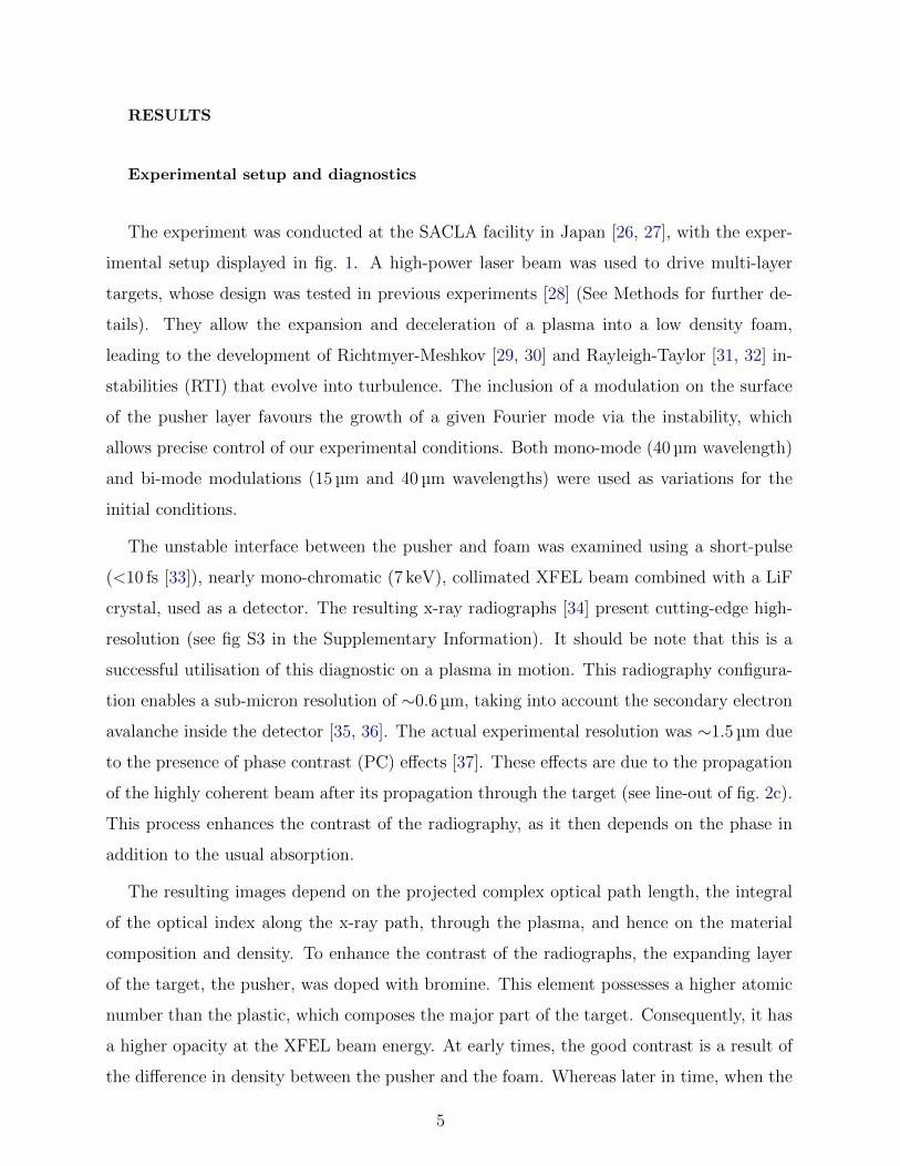
As can be seen in the dynamics shown in figure 3, the transition happens at earlier times

for bi-mode targets (around 40 ns). This difference might be due to the enhancement of non-

linear effects and mode coupling of a multi-wavelength perturbations [39]. This phenomenon

is highlighted on the 20 ns radiograph. The more pronounced non-linear effects can lead to a

quicker destabilisation of the flow, leading more rapidly to the turbulence, since the energy

injection happens at multiple wavelengths.

Simulations and dimensionless numbers

To ascertain the nature of the flow at late time, it is necessary to study not only its

spectrum, but also the actual plasma regime. One of the characteristics of a turbulent flow

is a high Reynolds number (Re) at the injection scale, for instance higher than 1.5 × 106

according to [40]. To calculate this number, the characteristic length (L), velocity (u) and

viscosity (ν) of the flow are mandatory. Except for L, these parameters can not be obtained

from the radiography and so simulations were performed to determine their value at the

6

beginning of the turbulent phase.

The 2D hydrodynamic simulations, performed with the FLASH4 code, globally reproduce

the evolution of our plasma flow up to the beginning of the turbulent phase. In particular,

the morphology of the interface, its position and the RTI growth are correctly reproduced up

to 50 ns (see fig S1 and fig S2 of the Supplementary). However, the observed blurry aspect

is not recreated in simulations, which make them inappropriate for the detailed study of the

turbulent-like phase. This might be due to the coarse resolution or to the absence of direct

dissipation mechanism (Euler equations). Indeed, the simulations are limited in resolution

and do not reach the dissipation scale, thus limiting the effective Reynolds number of the

simulations (Re = (L/η)4/3, see the following discussion or method for limitations). The

absence of the third dimension in the simulations could also contribute (see section II of the

Supplementary).

Based on their similarities with the experiment, the simulations were deemed sufficient to

determine various physical parameters (temperature, density, pressure, fluid velocity), which

were not determined experimentally. These values were taken at 50 ns, i.e just prior to the

beginning of the turbulent phase, to calculate the characteristic dimensionless numbers.

However, such calculations could not be performed during the turbulent phase since this

phase was not reproduced in simulations.

The simulated values, as well as some derived parameters are presented in table I. The

viscosity, required for the Reynolds number, is calculated with the multi-material formula

established by Clerouin [41], which can be applied to partially ionised plasmas. A Thomas-

Fermi model is used to determine the ionisation of each species. These values are used to

estimate the Reynolds number at the beginning of the turbulent phase, which is found to

be of the order of 107. This high value, rarely attained in simulations due to numerical

viscosity, is consistent with turbulence theory [40].

Alternative approaches can be taken to calculate the Reynolds number at 50 ns. They

mainly differ in their definition of the characteristic velocity and length of energy injection.

For instance, an upper value of the Reynolds number can be calculated using the actual

plasma extension as well as the fluid velocity (see table I). In this case, it will be equal

to 6 × 107. We can also use the mixing zone of the RTI and its growth velocity, which is

actually equivalent to the fluid velocity in the reference frame of the interface (see table II).

With this more common definition, the Reynolds number drops to 1 × 107. Finally, if we

7

consider the spacing between RTI spikes and the variation of fluid velocity in the lateral

direction as a constraint for our system, we find Re∼7 × 106 (see last column of table II).

These choices give roughly the same order of magnitude for Re and all remain consistent

with turbulence theories.

Spectral analysis

In order to experimentally study the turbulent phase, which appears in late time radio-

graphs, regions of interest (ROI) were defined in which the flow appears to be turbulent (see

red squared on 3). A spectral analysis of each ROI was performed. To this end, the mean

radial power spectrum of ROIs was determined (see method), assuming isotropy. While this

is a very good approximation during the turbulent phase, this breaks down at early times

(see fig. 2 and the spectral analysis section of the Supplementary). Images of the XFEL

beam itself, radiographs of non-driven target, unshocked foam in driven shots, and early

time results, were also analysed as references.

The obtained intensity spectrum can be linked to the imaginary part of the optical length.

At early times, it relates to a density spectrum. Later in time, in the turbulent phase, the

density tends to become homogeneous, and so the intensity spectrum indicates the bromine

concentration. Given our experimental conditions, the post-shock flow is subsonic and as a

consequence the density fluctuations and the velocity spectrum should be the same [42, 43].

In other words, at early times, the density fluctuations (or more precisely the volumetric

x-ray attenuation) should behave as a passive scalar, which is transported with the flow.

At later times, the bromine concentration is the passive scalar, which is transported. The

presence of PC may also alter the obtained spectrum. However, only high spatial frequencies

may be affected, since the longest PC wavelength measured for high optical index gradient

is of the order of 3 µm (see supplementary information).

Typical spectra can be decomposed into four zones, as shown in fig. 4. For the lower

wave numbers (<2 × 10−1 µm−1) we can distinguish two spectral distributions. We qualify

them as “low” and “middle” spectra, with an inflection at a knee spatial frequency, fk. At

higher wave numbers, a bump appears at late times, during the turbulent phase. For very

high spatial frequency, f , the spectra become almost flat with some noise. This corresponds

to the resolution limit of the radiography (∼1.5 µm).

8

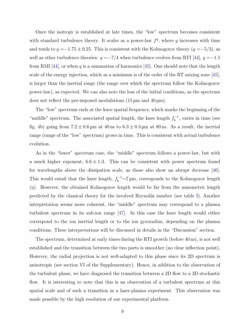
Once the isotropy is established at late times, the “low” spectrum becomes consistent

with standard turbulence theory. It scales as a power-law f q, where q increases with time

and tends to q =−1.75 ± 0.25. This is consistent with the Kolmogorov theory (q =−5/3), as

well as other turbulence theories: q =−7/4 when turbulence evolves from RTI [44], q =−1.5

from RMI [44], or when q is a summation of harmonics [45]. One should note that the length

scale of the energy injection, which as a minimum is of the order of the RT mixing zone [45],

is larger than the inertial range (the range over which the spectrum follow the Kolmogorov

power-law), as expected. We can also note the loss of the initial conditions, as the spectrum

does not reflect the pre-imposed modulations (15 µm and 40 µm).

The “low” spectrum ends at the knee spatial frequency, which marks the beginning of the

“middle” spectrum. The associated spatial length, the knee length f−1k , varies in time (see

fig. 4b) going from 7.2 ± 0.6 µm at 40 ns to 6.3 ± 0.3 µm at 80 ns. As a result, the inertial

range (range of the “low” spectrum) grows in time. This is consistent with actual turbulence

evolution.

As in the “lower” spectrum case, the “middle” spectrum follows a power-law, but with

a much higher exponent, 6.6 ± 1.3. This can be consistent with power spectrum found

for wavelengths above the dissipation scale, as those also show an abrupt decrease [46].

This would entail that the knee length, f−1k ∼7 µm, corresponds to the Kolmogorov length

(η). However, the obtained Kolmogorov length would be far from the nanometric length

predicted by the classical theory for the involved Reynolds number (see table I). Another

interpretation seems more coherent, the “middle” spectrum may correspond to a plasma

turbulent spectrum in its sub-ion range [47]. In this case the knee length would either

correspond to the ion inertial length or to the ion gyroradius, depending on the plasma

conditions. These interpretations will be discussed in details in the “Discussion” section.

The spectrum, determined at early times during the RTI growth (before 40 ns), is not well

established and the transition between the two parts is smoother (no clear inflection point).

However, the radial projection is not well-adapted to this phase since its 2D spectrum is

anisotropic (see section VI of the Supplementary). Hence, in addition to the observation of

the turbulent phase, we have diagnosed the transition between a 2D flow to a 3D stochastic

flow. It is interesting to note that this is an observation of a turbulent spectrum at this

spatial scale and of such a transition in a laser-plasma experiment. This observation was

made possible by the high resolution of our experimental platform.

9

The main difference between our measured spectrum and any theory is the presence of

the bump. It corresponds to a structure with a spatial scale of 3.9 ± 0.1 µm, which is smaller

than the knee length. This structure becomes more pronounced at later times (see fig. 4

c) and is absent at early ones. Thus, we can not associate this structure to an effect of the

PC. This is because PC effects should be more important at early times, when the gradient

of optical indexes is higher. Furthermore, we can also distinguish a smaller bump, whose

spatial frequency corresponds to the dimension of the measured PC (∼3 µm red arrow).

Therefore, the bump seems to be linked to the turbulent flow.

Such an observation is unprecedented and this “bump” structure is not predicted by

purely hydrodynamic turbulence theory. It may be the result of energy injection at a given

spatial scale, possibly due to non-local energy transport such as magnetic coupling (the

eddies increase magnetic fields by the dynamo effect [43]), or it might be linked to the near

resolution limit. A full explanation of this feature, however, is beyond the scope of this

article.

This experiment represents a milestone in HEDP study, as it is a direct experimental

measurement of the turbulent spectrum over a large order of spatial frequency and down

to microscopic scale, in a laser produced plasma experiment. It reveals characteristics (in-

flexion and bump), which, to our knowledge, have never been experimentally observed in

a controlled environment. The numerous features, observed here, are essential for bench-

marking models and simulations of plasma turbulence in HED systems. Moreover, with our

platform, suitably designed experiments could solve outstanding problems in HEDP either

in ICF or in astrophysics, where turbulence is of central importance.

DISCUSSION

Two particular features of the previously shown spectra are worth discussing since they

diverge from the usual turbulence theories. Those are the inflexion between the “low” and

“middle” spectra (knee) as well as the “bump”. Despite our lack of definitive explanation

for those features, we can provide some substantiated hypotheses.

As previously alluded to during the spectra description, the knee length could correspond

to the Kolmogorov length or to an ion characteristic length. For both cases there are

arguments promoting and opposing them. A point in common for both arguments is the

10

sudden drop in the power spectrum for spatial frequency above fk (“middle” spectrum),

although this, in itself, is insufficient. Two others points are worth considering: the actual

value of the knee length compared to its theoretical counterpart, and the temporal evolution

of this value.

Starting with the value of the knee length, one can rule out the possibility of it being the

Kolmogorov length. Indeed, the knee length evolves between 7.5 µm and 6.0 µm; this value

is far from the usual few nanometers of the Kolmogorov length. The theoretical Kolmogorov

length of our system is lower than a nanometer (see table I and II) according to the classical

turbulence theory (scaling as Re−3/4 see Method). Although this theoretical approach relies

on ideal hydrodynamics, whose approximations are not be perfectly valid in this case, the

actual Kolmogorov length should not be three orders of magnitude higher.

In the case of ionic effects, the transition between inertial range and sub-ionic range would

either happen at the ion inertial length when the plasma β is lower than 1 or at the ion

gyroradius when it is higher than 1 [47]. According to the values reported in table I and II,

the ion inertial length seems similar to the measured knee length. However the β parameter

of our system should be much higher than 1, given our estimations of the magnetic field

generated by Biermann battery effect (see Method and section IV of the Supplementary).

Furthermore, the ion gyroradius of our system should be of the order of a few millimetres,

or more, given our low magnetic field. So this explanation does not match well.

The second point to consider is the temporal variation of the knee length. As previously

described, this length seems to weakly decrease during the experiment. According to [48], in

the case of turbulence evolving from a RTI, the Kolmogorov length evolves as h−1/8, with h

the RTI amplitude or mixing zone width. In the most commonly studied case, this amplitude

evolves as t2 during the asymptotic regime of the RTI. This leads to a Kolmogorov length

evolution as t−1/4. Such evolution would agree with our knee length evolution, however our

mixing does not follow this kind of growth (see fig S2 in Supplementary). In our case, we

would rather expect an evolution as t−a/8 with 0 < a . 1. Furthermore, we should note

that in Ref [48], the viscosity is taken to be constant as a hypothesis. This does not seem

to be the case in our experiment according to our simulations and resulting calculations.

Thus, the above mentioned theoretical evolution might not be perfectly suitable in this

experiment. This is supported by our simulation results, from which we predict a quasi-

constant Kolmogorov length (see grey dotted curve on fig 4b).

11

According to our simulations, the ion inertial length should grow in time (see green dash-

dotted curve on fig 4b). So even if its value may correspond to the knee position at ∼50 ns,

it does not share its dynamic evolution. One might argue that our simulations can no longer

be fully trusted after the beginning of the turbulent phase, but the growth of the ion inertial

length start before. After considering these arguments, we are therefore still not able to

definitively understand the nature of the inflexion point.

As mentioned previously, the bump is an unexpected feature of the spectra, which be-

comes more pronounced in time. Its characteristic length, ∼3.9 ± 0.1 µm, does not corre-

spond to the effect of PC nor to any other diagnostic-based effects. Considering the existing

turbulence theories and current experiment and simulations, this bump could call some 2D

turbulence spectra to mind [49, 50]. For such spectra, a bump appears between the direct

cascade, which transports the energy to the smaller spatial scale, and the indirect cascade,

which transports the energy to the higher scale (a specificity of 2D turbulence). The bound-

ary between both cascades corresponds to the energy injection scale, which is marked by a

bump in the energy spectrum.

Following this comparison, the bump may correspond to a length characteristic of an

energy injection in the system. However the nature of such injection remains a mystery. The

main source of energy for the system is the optical laser. Despite its large focal spot (240 µm),

which can not be associated with the bump, it possess numerous smaller perturbation in the

form of speckles. However the bump appears only at late times, whereas the laser is shut

down after 4.5 ns. So it does not seems that they could be directly linked.

One of the particularities of the observed turbulence is that it happens within a plasma

flow, and such flows can be subject to electromagnetic constraints. Initially, there is no

pre-imposed magnetic field. The magnetic field produced by the laser and its interaction

with the target should disappear with the laser. However magnetic fields can be produced

as a result of plasma dynamics. According to our estimation (see method for the details), a

magnetic field of ∼0.1 G is produced around the interface position due to Biermann battery

effects (this is an overestimation of its actual value). Because of its low value, the magnetic

pressure is negligible compared to the thermal pressure; i.e. the β of the plasma is high. The

magnetic Reynolds number of the system is also relatively low (see methods). As a result,

the magnetic field diffuses in the plasma. It might still carry energy between spatial scales,

but its efficiency should also be low. Another downside of this explanation is understanding

12

the scale of the energy injection. Indeed, we do not explain why a self-generated magnetic

field would present such a specific spatial scale.

Another interpretation would be to think of the bump as an artefact of our experiment

and diagnostic. We have already ruled-out the possibility of a PC effect, but one could imag-

ine other lengths, which characterise our target, or the materials present (for instance the

pusher granularity or the size of the pore in the foam) might be responsible. However, these

lengths are already present from the beginning and thus there is no reason for the bump to

appears only later in time. However the only sound evidence for this would be obtained by

redoing the experiment with a different target design. For instance by using other materi-

als processing techniques, the granularity of the target will change, and the use of different

foams density will change the pore size. This will be the subject of an upcoming experiment.

It is worth mentioning that the experimental technique presented here can be applied

to other systems unrelated to turbulence. The high spatial and temporal resolution of

our diagnostic, its large field of view, as well as the monochromaticity of the XFEL beam

are assets, from which the laser plasma community will largely benefit. The possibilities

are numerous: from studying small details of physical phenomena (subtle morphology of

diverse instabilities and the effect of magnetic fields on them, separation of the elastic and

plastic wave in a shock) to the measurement of the actual plasma density using the XFEL

monochromaticity (possible application for the measurement of equation of state, or heat

transport...). The main down-side of this experimental technique is the requirement to

couple an XFEL to an optical high power laser and the rarity of such facilities. However

actively development is being performed at LCLS, SACLA and Eu-XFEL, where an external

magnetic field will also be added.

13

METHODS

Target composition

The target used during this experiment is similar to a previously tested target [28]. This is

a multi-layer target composed of a 10 µm parylene ablator, a 40 µm modulated brominated

plastic (C8H7Br) pusher and a resorcinol formaldehyde (C15H12O4) foam (100 mg cm−3).

The experiment was performed in SACLA experimental hutch 5. An optical laser deposits

approximately ∼20 J on a ∼240 µm diameter focal spot, which is smoothed by a hybrid

phase plate (HPP), in a ∼4.3 ns square pulse giving an intensity of ∼1 × 1013 W cm−2 on

target. This leads to the ablation of the first layer, the ablator, and in reaction generates a

shock wave inside the solid target. The shock wave, during its propagation, puts into motion

the rest of the target, in particular the pusher that expands into the foam and decelerates.

This situation is Rayleigh-Taylor unstable.

Most of the pushers were modulated in order to make this experiment reproducible and

easy to simulate. Indeed, this allows the control over which spatial modes will be favoured

during Rayleigh-Taylor development. These modes will not be created randomly due to

thermal noise, material roughness, imperfection in the spatial deposition of the laser energy,

or numerical noise, in the case of simulation. Two kinds of modulation were used: a simple

sine wave (mono-mode), with 40 µm wavelength and 5 µm amplitude; the sum of two sine

waves (bi-mode), the previous one and another with 15 µm wavelength and 5 µm amplitude.

Imagery technique

The imaging system consists of a collimated x-ray beam and a LiF crystal. When irradi-

ated by x-rays the LiF creates colour centres (CCs) that can be read out using a conventional

confocal fluorescent microscope [23]. Here, the XFEL beam consists of a short pulse (less

than 10 fs) x-ray burst centred on a 7 keV peak, with a ∼30 eV full width at half maximum

(FWHM) [33]. It is collimated so the resulting radiography images on the LiF have the

same dimension as the imaged object (contact radiography, i.e. magnification of 1). The

intrinsic resolution of this system depends on the spacing of the colour centres within the

LiF (a few nanometres), the resolution of the confocal microscope used to read out the data

14

(0.26 µm), and the secondary electron avalanche and diffusio of colour centres, that appear in

the LiF [35]. This last aspect seems to be the limiting factor in this experiment, as [36] sug-

gested the formation of a ∼0.6 µm diameter electron cloud in a similar configuration (XFEL,

with an energy of 10 keV). In this experiment, the image contrast is ensured initially by

the difference of density of the different materials involved (initially the foam is more than

ten times lighter than the pusher), then by the difference in the absorption coefficients of

those materials (the high Z material, Br, absorbs more x-rays), and by phase contrast (PC)

effects. The PC effects lead to the appearance of structures which were measured to be

≤3 µm, the upper limit corresponding to a static case, i.e. with no laser drive, on a 400

line per inch gold grid. This estimation was obtained through direct measurement of the

structure (radiography of the grid, observation of the tip of the RTI peaks), by line-outs,

and also by performing our spectral analysis, based on fast Fourier transforms, on those

line-outs. These three methods were applied on locations were PC was obvious, such as

the limit between the foam and the pusher. The PC structures do not correspond to the

measured bump wavelength, all structures spatially larger than 3 µm are due to absorption

effects.

Spectrum calculation

To determine the power spectrum, several steps were required. First the regions of

interest (ROIs) where cropped from the figure; they correspond to regions either completely

included in the shocked regions or entirely outside (unperturbed foam) used as reference.

The typical size of the ROIs were 520x520 pixels with a pixel size of 0.31 µm, although some

other dimensions (720x720, 1040x1040...) were used for checking the method consistency.

A fast Fourier transform was applied to the ROI, and the square of its norm taken. This

corresponds to the 2D power spectrum. These spectra were projected onto polar coordinates

and averaged over the angle to obtain a radial power spectrum (see fig. 4 for typical results).

An average over the radius was also performed to verify the isotropy of the system (see fig S6

in the Supplementary). Only the data taken after 30 ns are isotropic. Finally, the method

was applied on higher magnification images with a pixel size of 0.155 µm to ensure the

absence of artefacts due to the specific configuration of the microscope.

15

Simulations of the experiment

As described in the main part of the article, we used some hydrodynamic simulations

to obtain most of the physical parameters that characterise our plasma. Two radiative

hydrodynamic codes, with laser matter interaction module, were used: FLASH4 and MULTI.

FLASH4 (version 4.5 in this article), which is developed at the Flash Center (University of

Chicago) [24, 25], is a multidimensional hydrodynamic and magneto-hydrodynamic Eulerian

code with an adaptive mesh refinement (AMR) scheme. We used it in a 2D Cartesian

configuration over an 400x800 µm domain for a maximal resolution of ∼0.8 µm. This code

was used both in hydrodynamic, solving the Euler equations of fluids dynamic, and magneto-

hydrodynamic without any external magnetic field modes, both configuration returning

similar results (see table II).

MULTI [51] is a 1D Lagrangian code. Thank to both aspects, the resolution of the

performed simulations are higher than with FLASH4. However the global morphology of

the plasma flow can not be studied (only 1D).

For both types of simulation, the laser intensity is used as an adjustment parameters to

reproduce the initial interface velocity. The resulting simulations can be directly compared

to our experimental results with good adequacy (see Supplementary Information). However,

the turbulent phase was not reproduced. Thus the simulation results are no longer valid

after the beginning of the turbulent phase.

Calculation of Reynolds number

For the Reynolds number calculation (Re = uL/ν), the characteristic length, L, veloc-

ity, u, and viscosity, ν, are needed. The foam viscosity was calculated using the Clerouin

formula, which requires the shocked foam temperature (∼1 eV), its density (∼0.2 g cm−3),

its composition and ionisation (calculated through a Thomas-Fermi model). To determine

these parameters, we used the above mentioned simulations performed with the FLASH4.

We should note that the temperature and density obtained through simulation were simi-

lar to the ones given by the equation of state tables for our measured shock velocity. The

characteristic length and velocity can be either taken to correspond to [40]: the plasma

extension and bulk velocity, the RTI extension and the associated growth velocity, or the

16

inter-spikes extension and the lateral velocity. The exact definition depends on which scale

we consider for energy injection. The first possibility would usually be taken in jet like

objects (the global morphology of our expanding plasma), whereas the second and third are

more usually used for theoretical study of the RTI and resulting turbulence (usually it is

associated with periodic boundaries). We should note that the spacing between spikes grows

in time as they diverge from one another due to the curvature of the expanding plasma. In

the case of bulk flow, the length is taken to be equal to the plasma expansion: ∼400 µm at

50 ns. The velocity was taken to be the post-shock fluid velocity in the foam (∼7 km s−1).

The resulting Reynolds number is of the order of 107, which is consistent with turbulence

theories (other possibles values are written in table II).

Another estimation of the Reynolds number is possible by using some properties of the

turbulent spectrum. In the classical theory, which does not apply in our case (our experiment

is neither purely hydrodynamic nor incompressible), the Reynolds number is linked to the

injection spatial scale, `, and to the Kolmogorov scale, η, by the formula Re = (`/η)4/3.

Since we do not measure η in our experiment, we can use this formula to calculate the

actual dissipation scale. Here, we obtain a Kolmogorov scale of the order of a nanometer

(see table I and II, and section III of the Supplementary).

Magnetic field

The calculation of the magnetic field present in the plasma and related parameters is nec-

essary to evaluate its effect on the spectra. In this experiment no external magnetic fields

were directly applied on the target. The sole magnetic fields present are either produced by

laser-matter interaction (but they disappear after the laser pulse), or by the plasma evolu-

tion. Here we only consider magnetic fields produced by the Biermann battery effect. For

this, we calculate the cross product of the gradient of electronic temperature and electronic

density in the bubble at 50 ns using the simulations results. Using the Biermann battery

formula, we obtain a temporal variation of magnetic field of: ∂tB =∼2 mG ns−1. Supposing

that: this value is constant and that the magnetic field is advected with the plasma (stays

in the bubble), we calculate a magnetic field of ∼0.1 G after 50 ns. This is an overestimation

of the real magnetic field, as there is magnetic diffusion. Using this value and the Spitzer

formula to calculate the resistivity, we find a magnetic Reynolds number lower than 5 × 10−2

17

(no magnetic advection), a ion gyroragius of the order of 6.5 mm or more for a lower mag-

netic field, and a plasma beta much greater than 1. Further details and discussion can be

found in the Supplementary Information.

DATA AVAILABILITY

Raw data generated during the experiment (x-ray radiographs) are available from the

corresponding author on reasonable request.

REFERENCES

[1] Kolmogorov, A.N. The local structure of turbulence in incompressible viscous fluid for very

large Reynolds numbers. Proceedings: Mathematical and Physical Sciences 434, 9–13 (1991)

[2] Landau, L.D. and Lifshitz, E.M. Fluid mechanics (second edition): chapter III - turbulence.

Pergamon (1987)

[3] Zhou, Y. et al. Turbulent mixing and transition criteria of flows induced by hydrodynamic

instabilities. PoP 26, 080901 (2019)

[4] Boffetta, G. and Mazzino, A. Incompressible Rayleigh–Taylor turbulence. Annual Review of

Fluid Mechanics 49, 119–143 (2017)

[5] Srebro, Y. and Kushnir, D. and Elbaz, Y. and Shvarts, D. Modeling turbulent mixing in

inertial confinement fusion implosions. Laser and Particle Beams 21, 355–361 (2003)

[6] Thomas, V.A. and Kares, R.J. Drive asymmetry and the origin of turbulence in an ICF

implosion. PRL 109, 075004 (2012)

[7] Weber, C.R. et al. Inhibition of turbulence in inertial-confinement-fusion hot spots by viscous

dissipation. PRE 89, 053106 (2014)

[8] Martinez, D.A et al. Evidence for a Bubble-Competition Regime in Indirectly Driven Ablative

Rayleigh-Taylor Instability Experiments on the NIF. PRL 114, 215004 (2015)

[9] Casner, A. et al. From ICF to laboratory astrophysics: ablative and classical Rayleigh-Taylor

Instability experiments in turbulent-like regimes. Nuclear Fusion 59, 032002 (2018)

18

[10] Inoue, T. and Yamazaki, R. and Inutsuka, S. Turbulence and magnetic field amplification in

Supernova remnants: interactions between a strong shock wave and multiphase interstellar

medium. ApJ 695, 825–833 (2009)

[11] Roy, N. and Bharadwaj, S. and Dutta, P. and Chengalur, J.N. Magnetohydrodynamic tur-

bulence in supernova remnants. Monthly Notices of the Royal Astronomical Society: Letters

393, L26-L30 (2009)

[12] Radice, D. et al. Turbulence in core-collapse supernovae. Journal of Physics G: Nuclear and

Particle Physics 45, 053003 (2018)

[13] Mac Low, M.M. and Klessen, R.S. Control of star formation by supersonic turbulence. Rev.

Mod. Phys. 76, 125–194 (2004)

[14] Iffrig, O. and Hennebelle, P. Structure distribution and turbulence in self-consistently

supernova-driven ISM of multiphase magnetized galactic discs. A&A 604, A70 (2017)

[15] Federrath, C. The turbulent formation of stars. Physics Today 71, (2018)

[16] Evoli, C. and Yan, H. Cosmic ray propagation in galactic turbulence. The Astrophysical Jounal

782, 36 (2014)

[17] Holguin, F. et al. Role of cosmic-ray streaming and turbulent damping in driving galactic

winds. Monthly Notices of the Royal Astronomical Society 490, 1271-1282 (2019)

[18] Casner, A. Recent progress in quantifying hydrodynamics instabilities and turbulence in in-

ertial confinement fusion and high-energy-density experiments. Phil. Trans. R. Soc. A. 379,

20200021 (2021)

[19] Dubrulle, B. Beyond Kolmogorov cascades. Journal of Fluid Mechanics 867, P1 (2019)

[20] Beresnyak, A. MHD turbulence. Living Reviews in Computational Astrophysics 5, 2 (2019)

[21] White, T.G. et al. Supersonic plasma turbulence in the laboratory. Nature communications

10, 1758 (2019)

[22] Pikuz, T. et al. Development of new diagnostics based on LiF detector for pump-probe exper-

iments. Matter and Radiation at Extremes 3, 197–206 (2018)

[23] Faenov, A.Y. et al. Advanced high resolution x-ray diagnostic for HEDP experiments. Scien-

tific Reports 8, 16407 (2018)

[24] Fryxell, B. et al. FLASH: an adaptive mesh hydrodynamics code for modeling astrophysical

thermonuclear flashes. ApJS 131, 273–334 (2000)

19

[25] Dubey, A. et al. A survey of high level frameworks in block-structured adaptive mesh refine-

ment packages. Journal of Parallel and Distributed Computing 74, 3217–3227 (2014)

[26] Ishikawa, T. et al. A compact X-ray free-electron laser emitting in the sub-angstrom region.

Nature Photonics 6, 540—544 (2012)

[27] Tone, K. et al. Beamline, experimental stations and photon beam diagnostics for the hard

x-ray free electron laser of SACLA. New J. Phys. 12, 083035 (2013)

[28] Rigon, G. et al. Rayleigh-Taylor instability experiments on the LULI2000 laser in scaled

conditions for young supernova remnants. PRE 100, 021201 (2019)

[29] Richtmyer, R.D. Taylor instabilty in shock accelation of compressible fluids. Communication

on Pure and Applied Mathematics 13, 297–319 (1960)

[30] Meshkov, E.E. Instabilty of the interface of two gases accelerated by shock. Fluid Dynamics

4, 101–104 (1969)

[31] Rayleigh, J.W.S. Investigation of the character of the equilibrium of an incompressible heavy

fluid of variable density. Proceeding of the London Mathematical Society 14, 170–177 (1883)

[32] Taylor, G.I. The instability of liquid surfaces when accelerated in a direction perpendicular to

their planes. Proceeding of the Royal Society of London A201, 192–196 (1950)

[33] Inubushi, Y. et al. Measurement of the X-ray spectrum of a free electron laser with a wide-

range high-resolution single-shot spectrometer. Applied Sciences 7, 584 (2017)

[34] Mabey, P. et al. Characterization of high spatial resolution lithium fluoride X-ray detectors.

RSI 90, 063702 (2019)

[35] Grum-Grzhimailo, A.N. On the size of the secondary electron cloud in crystals irradiated by

hard X-ray photons. Eur. Phys. J. D 71, 69 (2017)

[36] Pikuz, T. et al. 3D visualization of XFEL beam focusing properties using LiF crystal X-ray

detector. Scientific Reports 5, 17713 EP (2015)

[37] Pikuz, T. et al. Propagation-based phase-contrast enhancement of nanostructure images us-

ing a debris-free femtosecond-laser-driven cluster-based plasma soft x-ray source and an LiF

crystal detector. Applied Optics 48, 6271–6276 (2009)

[38] Bian, X. et al. Revisiting the late-time growth of single-mode Rayleigh–Taylor instability and

the role of vorticity. Physica D: Nonlinear Phenomena 403, 132250 (2020)

[39] Xin, J. et al. Two mode coupling of the ablative Rayleigh-Taylor instabilities. Physics of

Plasmas 26, 032703 (2019)

20

[40] Dimotakis, P.E. The mixing transition in turbulent flows. Journal of Fluid Mechanics 409,

69–98 (2000)

[41] Robey, H.F. Effects of viscosity and mass diffusion in hydrodynamically unstable plasma flows.

PoP 11, 4123–4133 (2004)

[42] Zhuravleva, I. et al. The relation between gas density and velocity power spectra in galaxy

clusters: qualitative treatment and cosmological simulations. Astrophys. J. Lett. 788, L13

(2014)

[43] Tzeferacos, P. et al. Laboratory evidence of dynamo amplification of magnetic fields in a

turbulent plasmar. Nature Communications 9, 591 (2018)

[44] Zhou, Y. A scaling analysis of turbulent flows driven by Rayleigh–Taylor and Richt-

myer–Meshkov instabilities. PoF 13, 538–543 (2001)

[45] Soulard, O. and Grea, B.J. Influence of zero-modes on the inertial-range anisotropy of

Rayleigh-Taylor and unstably stratified homogeneous turbulence. Phys. Rev. Fluids 2, 074603

(2017)

[46] Saddoughi, S.G. and Veeravalli, S.V. Local isotropy in turbulent boundary layers at high

Reynolds number. Journal of Fluid Mechanics 268, 333–372 (1994)

[47] Kiyani, K. H. et al. Dissipation and heating in solar wind turbulence: from the macro to

the micro and back again. Philosophical Transactions of the Royal Society A: Mathematical,

Physical and Engineering Sciences 373, 20140155 (2015)

[48] Ristorcelli, J.R. and Clark, T.T. Rayleigh–Taylor turbulence: self-similar analysis and direct

numerical simulations. Journal of Fluid Mechanics 507, 213–253 (2004)

[49] Chertkov, M. et al. Dynamics of Energy Condensation in Two-Dimensional Turbulence. Phys-

ical Review Letters 99, 084501 (2007)

[50] Xia, H. et al. Spectrally condensed turbulence in thin layers. Physics of Fluids 21, 125101

(2009)

[51] Ramis, R. and Schmalz, R. and Meyer-Ter-Vehn, J. MULTI - A computer code for one-

dimensional multigroup radiation hydrodynamics. Computer Physics Communications 49,

475–505 (1998)

21

ACKNOWLEDGEMENTS

The authors would like to thank the technical staff of LULI, the team of SACLA EH5, as

well as D. Sagae, H. Ogura, K. Ishida and T. Matsuoka for their technical support. We thank

O. Soulard for discussion. The XFEL experiment was performed at the BL3 of SACLA with

approval of the Japan Synchrotron Radiation Research Institute (JASRI) (Proposal No.

2019A8037). This work was supported by the Agence Nationale de la Recherche (ANR)

in the framework of the TURBOHEDP project (ANR-15-CE30-0011), the Investissements

d’Avenir from the LabEx PALM (ANR-10-LABX-0039-PALM) and a CNRS grant for travel

expenses (GOtoXFEL). The CELIA authors acknowledge financial support from the ANR

in the frame of “the Investments for the future” Programme IdEx Bordeaux-LAPHIA (No.

ANR-10-IDEX-03-02). This work was also supported by KAKENHI (grant no. 16H02246

and no. 17K05729) from the Japan Society for the Promotion of Science (JSPS), and X-ray

Free Electron Laser Priority Strategy Program (contract 12005014 at Osaka University) and

Quantum Leap Program (JPMXS0118067246 and JPMXS0118070187) from the Ministry

of Education, Culture, Sports, Science, and Technology (MEXT). This work was granted

access to the HPC ressources of GENCI under the allocation 2017-A0030510298. Part of

the writing of the article was performed by G. Rigon as an JSPS International Research

Fellow (Postdoctoral Fellowships for Research in Japan). The work of JIHT RAS team

on x-ray radiography development and implementation was supported by the Ministry for

Science and Higher Education of the Russian Federation (topic #075-15-2020-785). S.M. also

acknowledges the support of Russian Foundation for Basic Research (grant #19-32-90142).

AUTHOR CONTRIBUTIONS

M.K., T.P., B.A. conceived the project which was designed by G.R. The SACLA exper-

iment was performed by B.A., T.V., V.B., N.O., Y.U., Y.I., K.K., N.K., R.K., K.M., K.S.,

M.Y., T.Y., T.T., M.K., A.C. Scanning the luminescence images were provided by T.P.

and S.M. The experimental results analysis and writing the manuscript was performed by

G.R. with small inputs from P.M., M.M., S.P., E.F., O.P., A.C., B.A., F.B., G.G. for the

manuscript. All authors reviewed the manuscript.

22

COMPETING INTERESTS

The authors declare no competing interests.

FIGURES

b

(Credit: Chandra: NASA/CXC/Univ. of Utrecht/J.Vink et al.; XMM-Newton: ESA/Univ. Of Utrecht/J.Vink et al.)

a

Optical Laser:● 4.5 ns square pulse● ~15-25 J on target

LiF crystal

Target assembly

XFEL beam● 8 fs FWHM● 7 keV

●

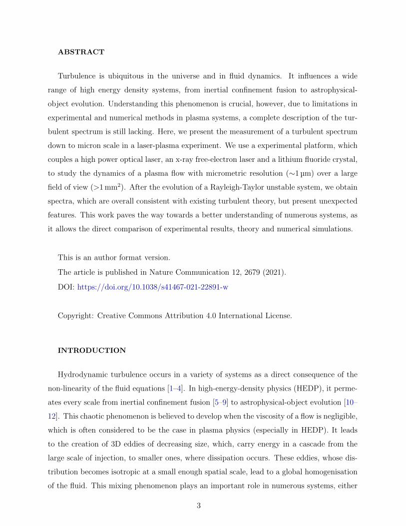
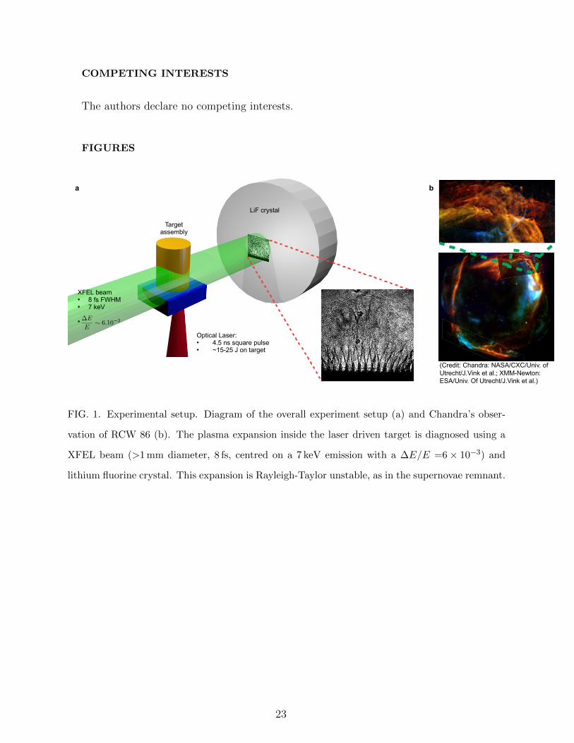
FIG. 1. Experimental setup. Diagram of the overall experiment setup (a) and Chandra’s obser-

vation of RCW 86 (b). The plasma expansion inside the laser driven target is diagnosed using a

XFEL beam (>1 mm diameter, 8 fs, centred on a 7 keV emission with a ∆E/E =6 × 10−3) and

lithium fluorine crystal. This expansion is Rayleigh-Taylor unstable, as in the supernovae remnant.

23

200 0 200[ m]

200

0

200

[m

]a

200 0 200[ m]

0

200

400

[m

]

b

c

0 20Distance [ m]

1.5

2.0

2.5

Valu

e [a

rb.u

nits

]

1.4 m

0 50 100 150[ m]

150

100

50[

m]

d

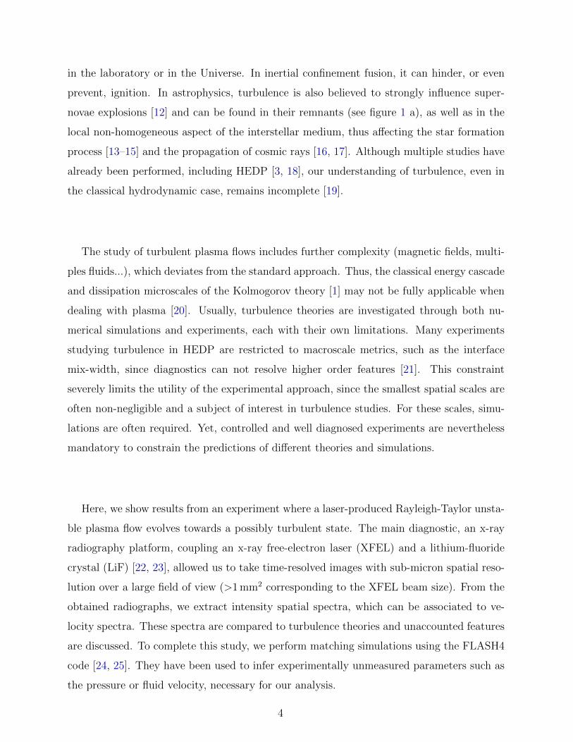
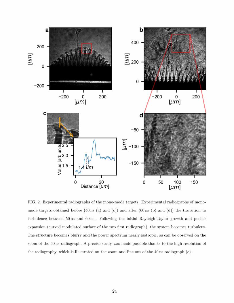
FIG. 2. Experimental radiographs of the mono-mode targets. Experimental radiographs of mono-

mode targets obtained before (40 ns (a) and (c)) and after (60 ns (b) and (d)) the transition to

turbulence between 50 ns and 60 ns. Following the initial Rayleigh-Taylor growth and pusher

expansion (curved modulated surface of the two first radiograph), the system becomes turbulent.

The structure becomes blurry and the power spectrum nearly isotropic, as can be observed on the

zoom of the 60 ns radiograph. A precise study was made possible thanks to the high resolution of

the radiography, which is illustrated on the zoom and line-out of the 40 ns radiograph (c).

24

FIG. 3. Experimental radiograph showing the dynamic of the bi-mode targets. The position of the

ROI taken to calculate the spectrum of figure 4 are shown with a red square.

25

40 50 60 70 80

Time (ns)

6

7

8

9

10

Knee

leng

th (µ

m)

t 1/4

1/f ion

. 104

b

0.2 0.3 0.4 0.5 0.6 0.7 0.8

Spatial frequency (µm 1)

101

Pow

er s

pect

rum

(arb

. uni

ts)

c80ns60ns50ns40ns20nsref

102

101

100

Spatial frequency (µm 1)

101

102

103

104

Pow

er s

pect

rum

(arb

. uni

ts)

f 5/3

resolution

bumpmiddle

f ionlowa

80ns60ns50ns40ns20nsref

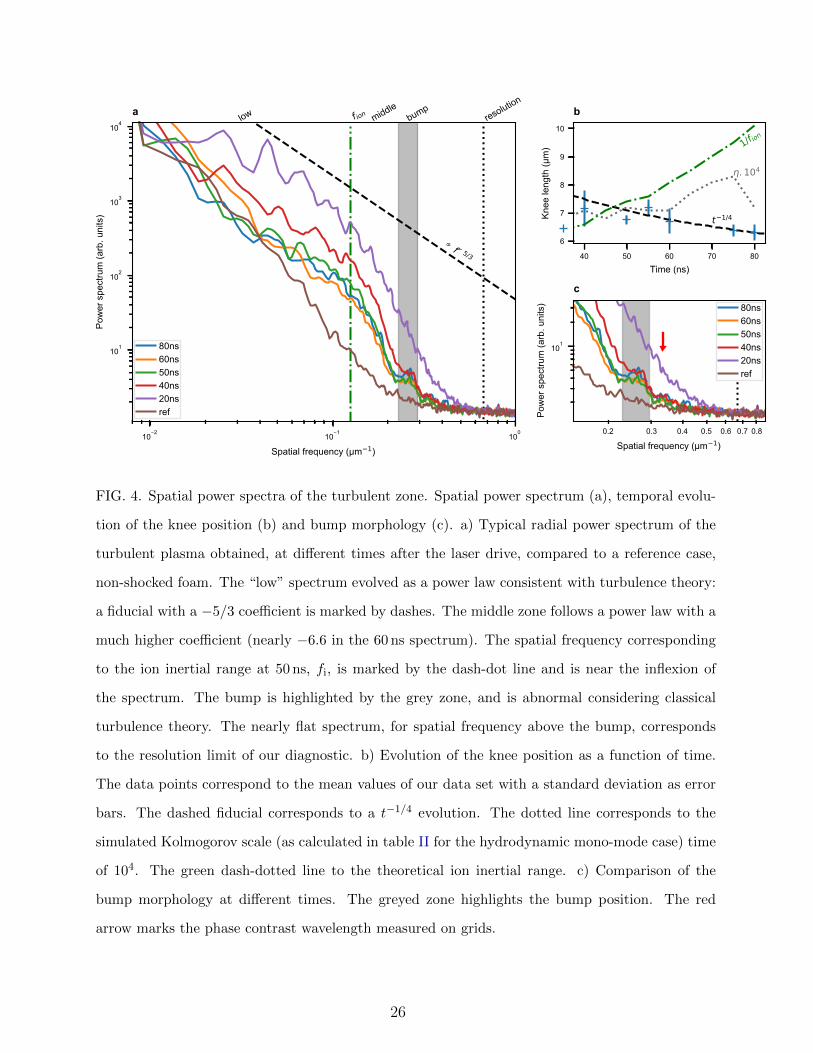
FIG. 4. Spatial power spectra of the turbulent zone. Spatial power spectrum (a), temporal evolu-

tion of the knee position (b) and bump morphology (c). a) Typical radial power spectrum of the

turbulent plasma obtained, at different times after the laser drive, compared to a reference case,

non-shocked foam. The “low” spectrum evolved as a power law consistent with turbulence theory:

a fiducial with a −5/3 coefficient is marked by dashes. The middle zone follows a power law with a

much higher coefficient (nearly −6.6 in the 60 ns spectrum). The spatial frequency corresponding

to the ion inertial range at 50 ns, fi, is marked by the dash-dot line and is near the inflexion of

the spectrum. The bump is highlighted by the grey zone, and is abnormal considering classical

turbulence theory. The nearly flat spectrum, for spatial frequency above the bump, corresponds

to the resolution limit of our diagnostic. b) Evolution of the knee position as a function of time.

The data points correspond to the mean values of our data set with a standard deviation as error

bars. The dashed fiducial corresponds to a t−1/4 evolution. The dotted line corresponds to the

simulated Kolmogorov scale (as calculated in table II for the hydrodynamic mono-mode case) time

of 104. The green dash-dotted line to the theoretical ion inertial range. c) Comparison of the

bump morphology at different times. The greyed zone highlights the bump position. The red

arrow marks the phase contrast wavelength measured on grids.

26

TABLES

Simulated Parameters Formula MULTI FLASH

Interface Position (L) [µm] simulated 388 410

Foam density (ρ) [g cm−3] simulated 0.2 0.22

Temperature (T ) [eV] simulated 1.1 0.8

Pressure (P ) [kbar] simulated 43 26

Fluid velocity (u) [km s−1] simulated 5.7 5.5

Calculated Parameters

Foam ionisation (ZC, ZH, ZO) Thomas-Fermia 0.9, 0.4 and 1 0.9, 0.4 and 1

Mean ionisation (Z) (15ZC + 12ZH + 4ZO)/31 0.7 0.7

Mean ion mass (mi) [10−23 g] (15mC + 12mH + 4mO)/31 1.37 1.37

Ion density (ni) [1022 cm−3] ρ/mi 1.38 1.60

Viscosity (ν) [10−4 cm2 s−1] Clerouin formula [41] 5 4

Reynolds (Re) uL/ν 4 × 107 6 × 107

Euler (Eu) P/(ρu2) 0.7 0.4

Kolmogorov length (η) [nm] L/Re3/4 0.7 0.6

Electron inertial length [nm] 5.31 × 105·n−0.5e 52 50

Ion inertial length [µm] 2.28 × 107/Z · (mi/(amu · ni))0.5 7.7 7.4

a Use of the program developed by Murillo Group from the Michigan State University. Those program

can be found on github: https://github.com/MurilloGroupMSU/Dense-Plasma-Properties-Database

TABLE I. Plasma Parameters. Summary of different plasma parameters relevant to the flow. The

“simulated parameters” are deduced from simulations. They are taken in the foam near the RTI

peak at the proximity of the interface. The “calculated parameters” are determined through the

formula (in cgs units, amu is the atomic mass unit) using the simulated parameters. Alternative

values for the parameters depending on L and u can be found in table II, where a more conventional

calculation method is used.

27

Parameters MHD bi-mode MHD mono-mode Hydro mono-mode Hydro lateral

Mixing Zone width (L) [µm] 120 105 134 65

Characteristic velocity (u) [km s−1] 1.5 2.1 2.9 4

Reynolds (Re) 5 × 106 6 × 106 1 × 107 7 × 106

Euler (Eu) 3.7 1.9 1.4 0.8

Kolmogorov length (η) [nm] 1.2 0.9 0.7 0.5

TABLE II. Alternative values of the Plasma Parameters. This table is an alternative of the value

found in table I when using the reference frame of the expanding interface. Since the values

presented here depend on the RTI development, only values obtained using the 2D simulations

(FLASH) are shown. The last column of the table corresponds to value taken in the transverse

direction. L is the spacing between spike and u the lateral variation of velocity. This values were

take from the hydrodynamic simulation of the mono-mode case.

28