Microsoft Excel 2010 - UQ Library · PDF fileReproduced or adapted from original content provided under Creative Commons license by The University of Queensland Library Microsoft Excel

Reproduced or adapted from original content provided under Creative Commons license by The University of Queensland Library

Microsoft Excel 2013 Manipulating Data

Course Objectives

Distinguish between relative and absolute cell references

Use IF function

Use the Vlookup function

Use PivotTable for flexible data presentation

Sort and filter to extract data

Staff Training (Bookings only) Student Training and Support

Phone (07) 3365 2666 Phone (07) 3365 8811 or 1300 738 082

Email [email protected] Email [email protected]

Web http://www.uq.edu.au/staffdevelopment Web http://www.library.uq.edu.au/ask-it/ Staff may contact their trainer with enquiries and feedback

related to training content.

Please contact Staff Development for booking enquiries or

your local I.T. Support for general technical enquiries.

UQ Students may contact the Library’s Ask

I.T. team for I.T. support related to the

Library and their studies.

http://www.library.uq.edu.au/

http://creativecommons.org/licenses/by-nc/3.0/au/

UQ Library

Staff and Student I.T. Training

2 of 17 Ask I.T. Microsoft Excel 2013: Manipulating Data

Table of Contents

Relative & Absolute Cell References ............................................................................. 3 AutoSum ................................................................................................... 3 Relative cell references ............................................................................. 3 Absolute cell references ............................................................................ 4

Date Calculations and Conditional Formatting ............................................................. 4 Date calculations ...................................................................................... 4 Apply conditional formatting ...................................................................... 5 Apply conditional formatting to a whole row .............................................. 5

Data Analysis ................................................................................................................... 6

‘IF’ Function ..................................................................................................................... 6 Using ‘IF’ statements ................................................................................ 6 Using nested ‘IF’ statements ..................................................................... 7

Lookup Functions ........................................................................................................... 7 Using V lookup.......................................................................................... 7

Pivot Table ....................................................................................................................... 8 Naming cells via ribbon ........................................................................... 8 Create a pivot table ................................................................................. 9 Add data to PivotTable .......................................................................... 10 Edit PivotTable ...................................................................................... 10 Create a PivotChart .............................................................................. 11

Sorting & Filtering Lists ................................................................................................ 12 Sort by single criteria............................................................................. 12 Sort by multiple criteria .......................................................................... 12 Filtering with AutoFilter .......................................................................... 13 Progressive filtering .............................................................................. 14

Find Unique Values and Remove Duplicates .............................................................. 15 Find unique values ................................................................................ 15

Protection ...................................................................................................................... 16 Worksheet protection ............................................................................ 16 Unprotected cells .................................................................................. 16

Goal Seek ....................................................................................................................... 17 Use ‘Goal Seek’ tool ............................................................................. 17

Exercise document: Go to http://www.library.uq.edu.au/ask-it/exercises and click the green Manipulate Data button to open Excel2010_exercisesLvl2.xlsx. Make sure you are on the Student Fees sheet.

http://www.library.uq.edu.au/ask-it/exercises

UQ Library


Notes


Relative & Absolute Cell References Adjust column widths to see headings.

AutoSum

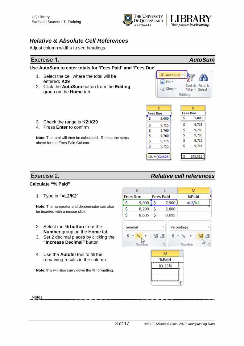
Use AutoSum to enter totals for ‘Fees Paid’ and ‘Fees Due’

1. Select the cell where the total will be entered: K29

2. Click the AutoSum button from the Editing group on the Home tab.

3. Check the range is K2:K29 4. Press Enter to confirm Note: The total will then be calculated. Repeat the steps

above for the Fees Paid Column.

Relative cell references

Calculate “% Paid”

1. Type in “=L2/K2” Note: The numerator and denominator can also

be inserted with a mouse click.

2. Select the % button from the Number group on the Home tab

3. Set 2 decimal places by clicking the “Increase Decimal” button

4. Use the Autofill tool to fill the remaining results in the column.

Note: this will also carry down the % formatting.

UQ Library


Notes


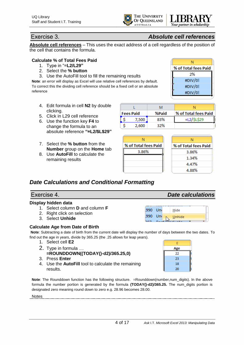
Absolute cell references

Absolute cell references – This uses the exact address of a cell regardless of the position of the cell that contains the formula. Calculate % of Total Fees Paid

1. Type in “=L2/L29” 2. Select the % button 3. Use the AutoFill tool to fill the remaining results

Note: an error will display as Excel will use relative cell references by default.

To correct this the dividing cell reference should be a fixed cell or an absolute

reference

4. Edit formula in cell N2 by double clicking.

5. Click in L29 cell reference 6. Use the function key F4 to

change the formula to an absolute reference “=L2/$L$29”

7. Select the % button from the Number group on the Home tab

8. Use AutoFill to calculate the remaining results

Date Calculations and Conditional Formatting

Date calculations

Display hidden data 1. Select column D and column F 2. Right click on selection 3. Select Unhide

Calculate Age from Date of Birth Note: Subtracting a date of birth from the current date will display the number of days between the two dates. To

find out the age in years, divide by 365.25 (the .25 allows for leap years). 1. Select cell E2

2. Type in formula ….

=ROUNDDOWN((TODAY()-d2)/365.25,0) 3. Press Enter 4. Use the AutoFill tool to calculate the remaining

results.

Note: The Rounddown function has the following structure. =Rounddown(number,num_digits). In the above

formula the number portion is generated by the formula (TODAY()-d2)/365.25. The num_digits portion is

designated zero meaning round down to zero e.g. 28.96 becomes 28.00.

UQ Library


Notes


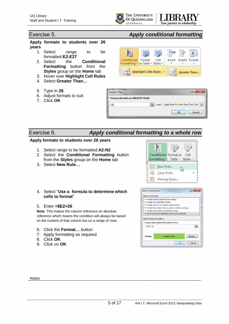
Apply conditional formatting

Apply formats to students over 26 years

1. Select range to be formatted:E2:E27

2. Select the Conditional Formatting button from the Styles group on the Home tab

3. Hover over Highlight Cell Rules 4. Select Greater Than…

5. Type in 26 6. Adjust formats to suit 7. Click OK

Apply conditional formatting to a whole row

Apply formats to students over 26 years

1. Select range to be formatted:A2:N2 2. Select the Conditional Formatting button

from the Styles group on the Home tab 3. Select New Rule…

4. Select “Use a formula to determine which cells to format”

5. Enter =$E2>26 Note: This makes the column reference an absolute

reference which means the condition will always be based

on the content of that column but on a range of rows

6. Click the Format… button 7. Apply formatting as required 8. Click OK 9. Click on OK

UQ Library


Notes


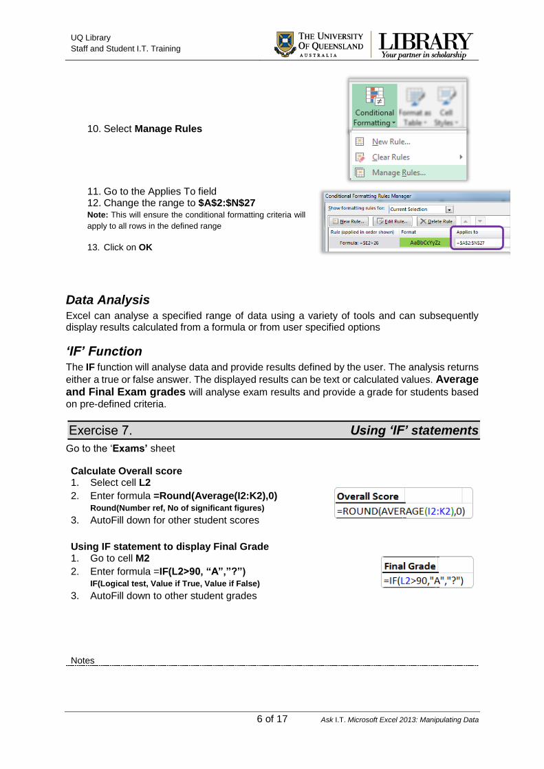
10. Select Manage Rules

11. Go to the Applies To field 12. Change the range to $A$2:$N$27 Note: This will ensure the conditional formatting criteria will

apply to all rows in the defined range

13. Click on OK

Data Analysis Excel can analyse a specified range of data using a variety of tools and can subsequently display results calculated from a formula or from user specified options

‘IF’ Function The IF function will analyse data and provide results defined by the user. The analysis returns

either a true or false answer. The displayed results can be text or calculated values. Average and Final Exam grades will analyse exam results and provide a grade for students based

on pre-defined criteria.

Using ‘IF’ statements

Go to the ‘Exams’ sheet

Calculate Overall score 1. Select cell L2

2. Enter formula =Round(Average(I2:K2),0) Round(Number ref, No of significant figures)

3. AutoFill down for other student scores

Using IF statement to display Final Grade 1. Go to cell M2

2. Enter formula =IF(L2>90, “A”,”?”) IF(Logical test, Value if True, Value if False)

3. AutoFill down to other student grades

UQ Library


Notes


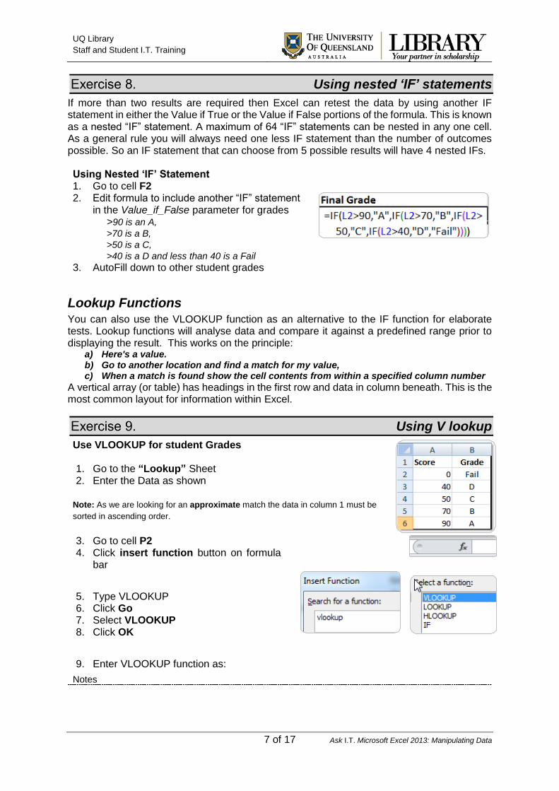
Using nested ‘IF’ statements

If more than two results are required then Excel can retest the data by using another IF statement in either the Value if True or the Value if False portions of the formula. This is known as a nested “IF” statement. A maximum of 64 “IF” statements can be nested in any one cell. As a general rule you will always need one less IF statement than the number of outcomes possible. So an IF statement that can choose from 5 possible results will have 4 nested IFs. Using Nested ‘IF’ Statement 1. Go to cell F2 2. Edit formula to include another “IF” statement

in the Value_if_False parameter for grades >90 is an A,

>70 is a B,

>50 is a C,

>40 is a D and less than 40 is a Fail

3. AutoFill down to other student grades

Lookup Functions You can also use the VLOOKUP function as an alternative to the IF function for elaborate tests. Lookup functions will analyse data and compare it against a predefined range prior to displaying the result. This works on the principle:

a) Here's a value. b) Go to another location and find a match for my value, c) When a match is found show the cell contents from within a specified column number

A vertical array (or table) has headings in the first row and data in column beneath. This is the most common layout for information within Excel.

Using V lookup

Use VLOOKUP for student Grades 1. Go to the “Lookup” Sheet 2. Enter the Data as shown

Note: As we are looking for an approximate match the data in column 1 must be

sorted in ascending order. 3. Go to cell P2 4. Click insert function button on formula

bar

5. Type VLOOKUP 6. Click Go 7. Select VLOOKUP 8. Click OK

9. Enter VLOOKUP function as:

UQ Library


Notes


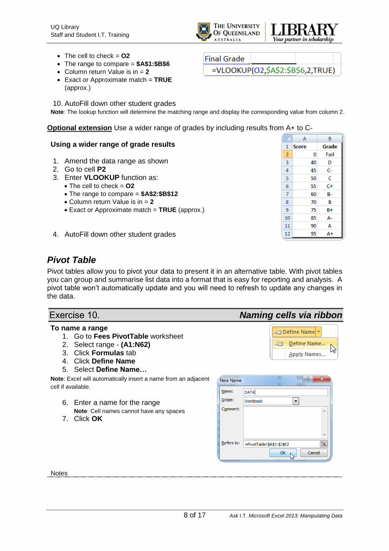
The cell to check = O2

The range to compare = $A$1:$B$6

Column return Value is in = 2

Exact or Approximate match = TRUE

(approx.)

10. AutoFill down other student grades

Note: The lookup function will determine the matching range and display the corresponding value from column 2. Optional extension Use a wider range of grades by including results from A+ to C- Using a wider range of grade results 1. Amend the data range as shown 2. Go to cell P2 3. Enter VLOOKUP function as:

The cell to check = O2

The range to compare = $A$2:$B$12

Column return Value is in = 2

Exact or Approximate match = TRUE (approx.)

4. AutoFill down other student grades

Pivot Table Pivot tables allow you to pivot your data to present it in an alternative table. With pivot tables you can group and summarise list data into a format that is easy for reporting and analysis. A pivot table won’t automatically update and you will need to refresh to update any changes in the data.

Naming cells via ribbon

To name a range 1. Go to Fees PivotTable worksheet 2. Select range - (A1:N62) 3. Click Formulas tab 4. Click Define Name 5. Select Define Name…

Note: Excel will automatically insert a name from an adjacent

cell if available.

6. Enter a name for the range

Note: Cell names cannot have any spaces 7. Click OK

UQ Library


Notes


Create a pivot table

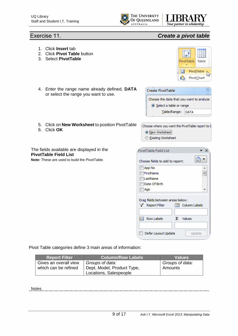
1. Click Insert tab 2. Click Pivot Table button 3. Select PivotTable

4. Enter the range name already defined, DATA or select the range you want to use.

5. Click on New Worksheet to position PivotTable 6. Click OK

The fields available are displayed in the PivotTable Field List Note: These are used to build the PivotTable.

Pivot Table categories define 3 main areas of information:

Report Filter Column/Row Labels Values

Gives an overall view which can be refined

Groups of data: Dept, Model, Product Type, Locations, Salespeople

Groups of data: Amounts

UQ Library


Notes


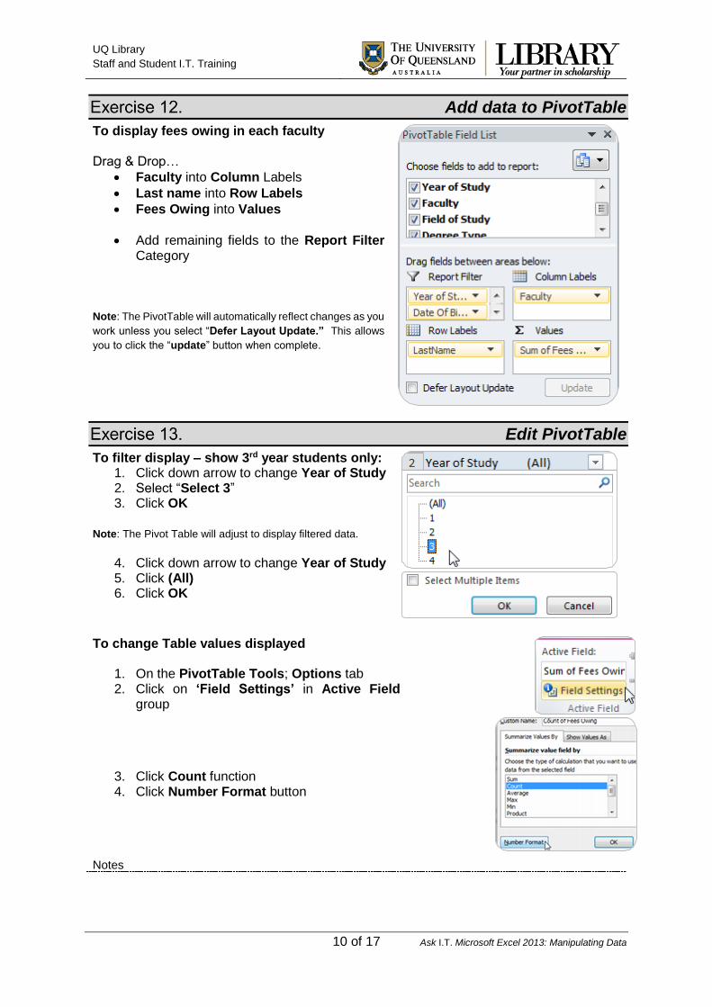
Add data to PivotTable

To display fees owing in each faculty Drag & Drop…

Faculty into Column Labels

Last name into Row Labels

Fees Owing into Values

Add remaining fields to the Report Filter Category

Note: The PivotTable will automatically reflect changes as you

work unless you select “Defer Layout Update.” This allows

you to click the “update” button when complete.

Edit PivotTable

To filter display – show 3rd year students only: 1. Click down arrow to change Year of Study 2. Select “Select 3” 3. Click OK

Note: The Pivot Table will adjust to display filtered data.

4. Click down arrow to change Year of Study 5. Click (All) 6. Click OK

To change Table values displayed

1. On the PivotTable Tools; Options tab 2. Click on ‘Field Settings’ in Active Field

group

3. Click Count function 4. Click Number Format button

UQ Library


Notes


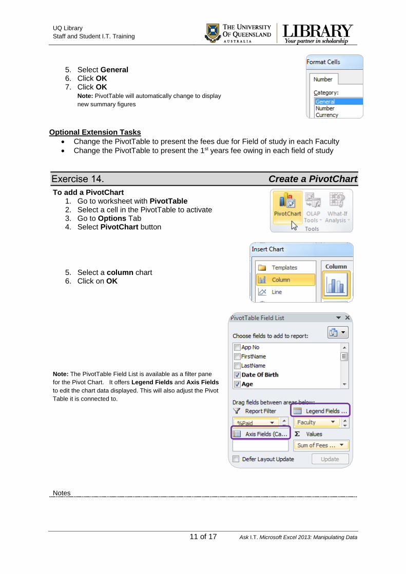
5. Select General 6. Click OK 7. Click OK

Note: PivotTable will automatically change to display

new summary figures

Optional Extension Tasks

Change the PivotTable to present the fees due for Field of study in each Faculty

Change the PivotTable to present the 1st years fee owing in each field of study

Create a PivotChart

To add a PivotChart 1. Go to worksheet with PivotTable 2. Select a cell in the PivotTable to activate 3. Go to Options Tab 4. Select PivotChart button

5. Select a column chart 6. Click on OK

Note: The PivotTable Field List is available as a filter pane

for the Pivot Chart. It offers Legend Fields and Axis Fields

to edit the chart data displayed. This will also adjust the Pivot

Table it is connected to.

UQ Library


Notes


Optional Extension Tasks

Change the PivotChart to present the Amount of Fees Owing in each Faculty by Degree Type

Change the PivotChart to present the number of students with fees owing in year by Degree Type

Sorting & Filtering Lists

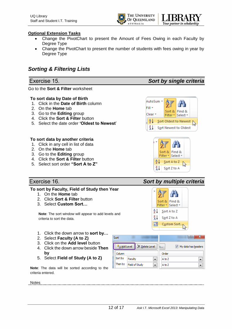
Sort by single criteria

Go to the Sort & Filter worksheet To sort data by Date of Birth 1. Click in the Date of Birth column 2. On the Home tab 3. Go to the Editing group 4. Click the Sort & Filter button 5. Select the date order ‘Oldest to Newest’

To sort data by another criteria 1. Click in any cell in list of data 2. On the Home tab 3. Go to the Editing group 4. Click the Sort & Filter button 5. Select sort order “Sort A to Z”

Sort by multiple criteria

To sort by Faculty, Field of Study then Year 1. On the Home tab 2. Click Sort & Filter button 3. Select Custom Sort…

Note: The sort window will appear to add levels and

criteria to sort the data.

1. Click the down arrow to sort by… 2. Select Faculty (A to Z) 3. Click on the Add level button 4. Click the down arrow beside Then

by 5. Select Field of Study (A to Z)

Note: The data will be sorted according to the

criteria entered.

UQ Library


Notes


Sorting Data allows you to present it in a specified order. If you want to extract data use the filtering tool available from AutoFilter.

Filtering with AutoFilter

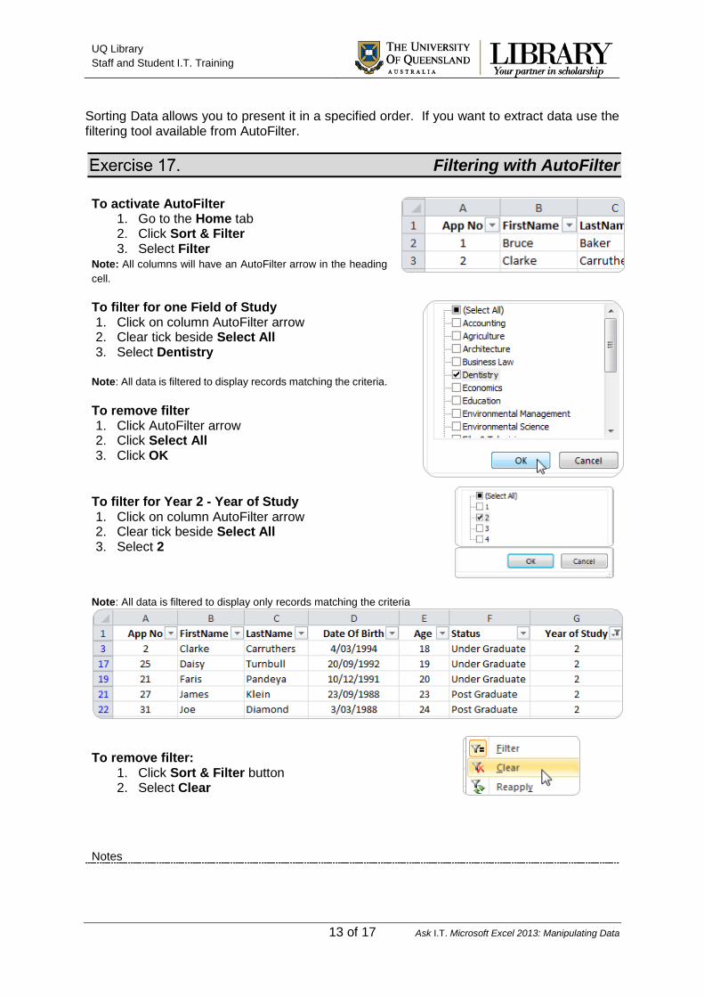
To activate AutoFilter

1. Go to the Home tab 2. Click Sort & Filter 3. Select Filter

Note: All columns will have an AutoFilter arrow in the heading

cell.

To filter for one Field of Study 1. Click on column AutoFilter arrow 2. Clear tick beside Select All 3. Select Dentistry

Note: All data is filtered to display records matching the criteria. To remove filter 1. Click AutoFilter arrow 2. Click Select All 3. Click OK

To filter for Year 2 - Year of Study 1. Click on column AutoFilter arrow 2. Clear tick beside Select All 3. Select 2

Note: All data is filtered to display only records matching the criteria

To remove filter:

1. Click Sort & Filter button 2. Select Clear

UQ Library


Notes


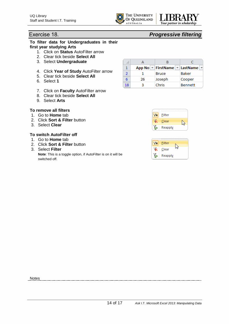
Progressive filtering

To filter data for Undergraduates in their first year studying Arts

1. Click on Status AutoFilter arrow 2. Clear tick beside Select All 3. Select Undergraduate

4. Click Year of Study AutoFilter arrow 5. Clear tick beside Select All 6. Select 1

7. Click on Faculty AutoFilter arrow 8. Clear tick beside Select All 9. Select Arts

To remove all filters 1. Go to Home tab 2. Click Sort & Filter button 3. Select Clear

To switch AutoFilter off 1. Go to Home tab 2. Click Sort & Filter button 3. Select Filter

Note: This is a toggle option, if AutoFilter is on it will be

switched off.

UQ Library


Notes


Find Unique Values and Remove Duplicates

Find unique values

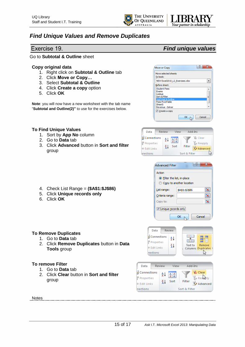
Go to Subtotal & Outline sheet Copy original data

1. Right click on Subtotal & Outline tab 2. Click Move or Copy… 3. Select Subtotal & Outline 4. Click Create a copy option 5. Click OK

Note: you will now have a new worksheet with the tab name

“Subtotal and Outline(2)” to use for the exercises below.

To Find Unique Values 1. Sort by App No column 2. Go to Data tab 3. Click Advanced button in Sort and filter

group

4. Check List Range = ($A$1:$J$86) 5. Click Unique records only 6. Click OK

To Remove Duplicates 1. Go to Data tab 2. Click Remove Duplicates button in Data

Tools group

To remove Filter

1. Go to Data tab 2. Click Clear button in Sort and filter

group

UQ Library


Notes


Protection To prevent a user from accidentally or deliberately changing, moving, or deleting important data from a worksheet or workbook, you can protect certain worksheet or workbook elements, with or without a password.

Worksheet protection

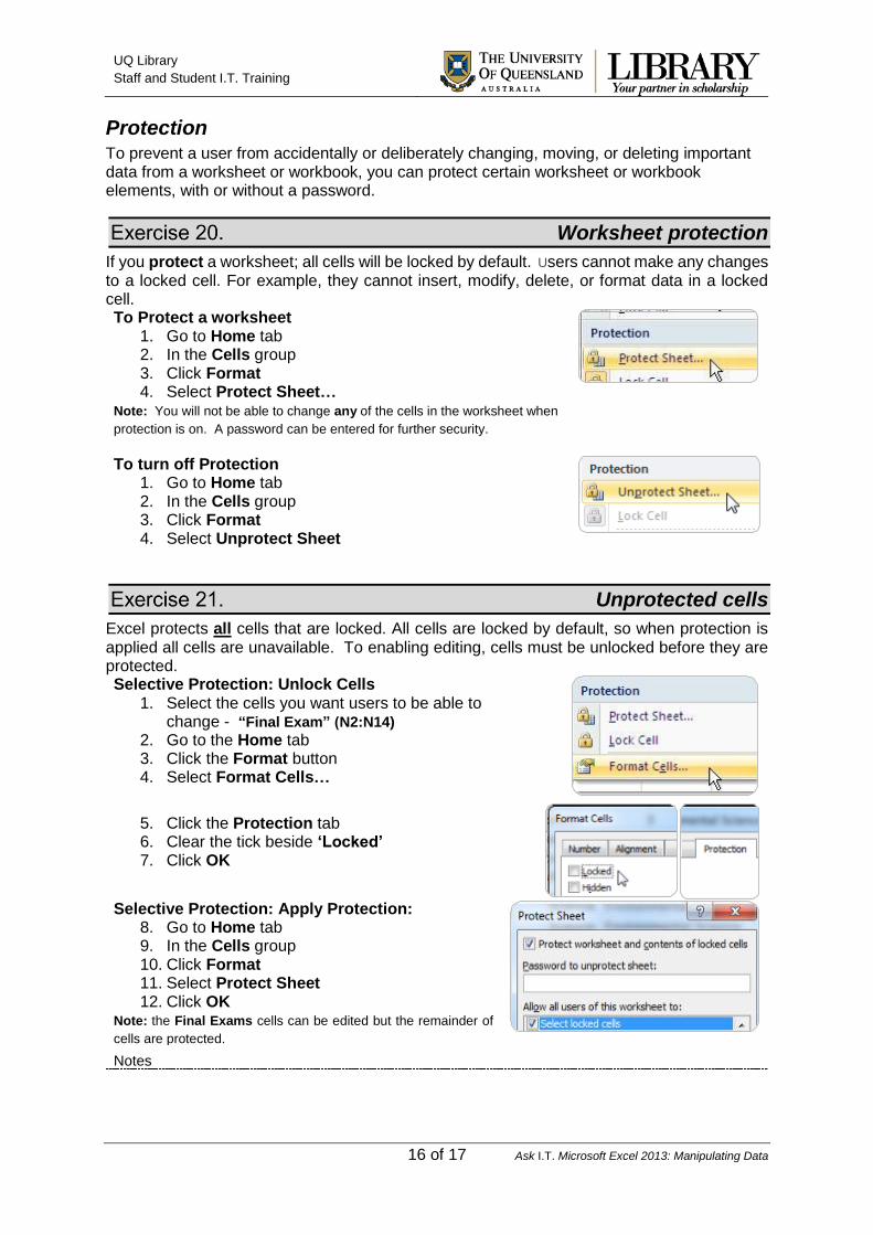
If you protect a worksheet; all cells will be locked by default. Users cannot make any changes to a locked cell. For example, they cannot insert, modify, delete, or format data in a locked cell. To Protect a worksheet

1. Go to Home tab 2. In the Cells group 3. Click Format 4. Select Protect Sheet…

Note: You will not be able to change any of the cells in the worksheet when

protection is on. A password can be entered for further security.

To turn off Protection 1. Go to Home tab 2. In the Cells group 3. Click Format 4. Select Unprotect Sheet

Unprotected cells

Excel protects all cells that are locked. All cells are locked by default, so when protection is applied all cells are unavailable. To enabling editing, cells must be unlocked before they are protected. Selective Protection: Unlock Cells

1. Select the cells you want users to be able to change - “Final Exam” (N2:N14)

2. Go to the Home tab 3. Click the Format button 4. Select Format Cells…

5. Click the Protection tab 6. Clear the tick beside ‘Locked’ 7. Click OK

Selective Protection: Apply Protection: 8. Go to Home tab 9. In the Cells group 10. Click Format 11. Select Protect Sheet 12. Click OK

Note: the Final Exams cells can be edited but the remainder of

cells are protected.

UQ Library


Notes


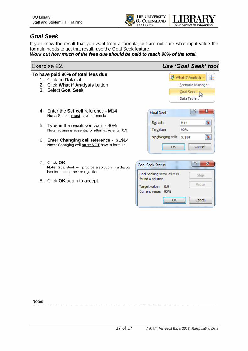
Goal Seek If you know the result that you want from a formula, but are not sure what input value the formula needs to get that result, use the Goal Seek feature. Work out how much of the fees due should be paid to reach 90% of the total.

Use ‘Goal Seek’ tool

To have paid 90% of total fees due 1. Click on Data tab 2. Click What if Analysis button 3. Select Goal Seek

4. Enter the Set cell reference - M14

Note: Set cell must have a formula

5. Type in the result you want - 90% Note: % sign is essential or alternative enter 0.9

6. Enter Changing cell reference - $L$14 Note: Changing cell must NOT have a formula

7. Click OK Note: Goal Seek will provide a solution in a dialog

box for acceptance or rejection

8. Click OK again to accept.

Documents

Microsoft Excel 2010 - UQ Library · PDF fileReproduced or adapted from original content provided under Creative Commons license by The University of Queensland Library Microsoft Excel