Microsoft Excel 2016 Fundamentals

Participant’s Guide

OTS Publication: ex1601 • 04/04/17 • Training@Towson.edu • Office of Technology Services © 2017 Towson University This work is licensed under the Creative Commons Attribution-NonCommercial-NoDerivs License.

Details available at http://www.towson.edu/OTStraining

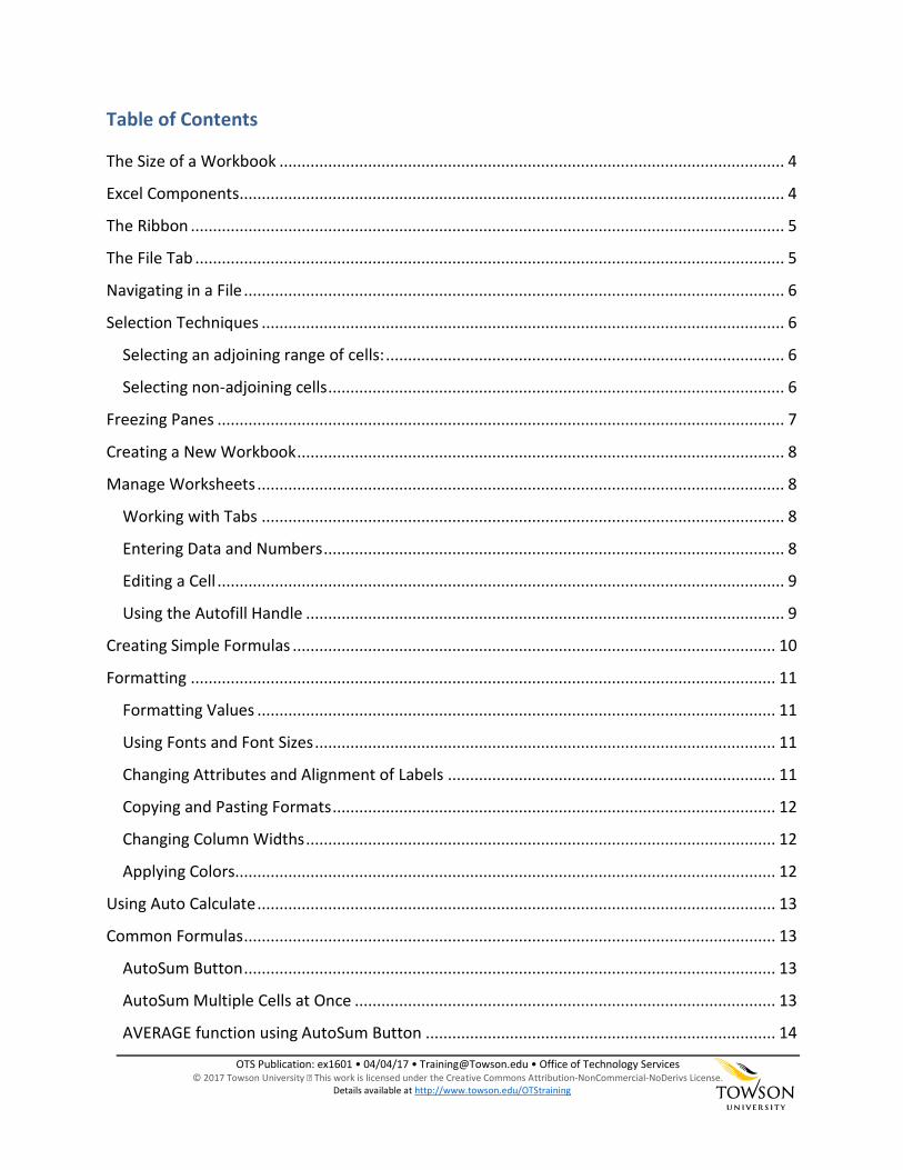
Table of Contents

The Size of a Workbook .................................................................................................................. 4

Excel Components ........................................................................................................................... 4

The Ribbon ...................................................................................................................................... 5

The File Tab ..................................................................................................................................... 5

Navigating in a File .......................................................................................................................... 6

Selection Techniques ...................................................................................................................... 6

Selecting an adjoining range of cells: .......................................................................................... 6

Selecting non-adjoining cells ....................................................................................................... 6

Freezing Panes ................................................................................................................................ 7

Creating a New Workbook .............................................................................................................. 8

Manage Worksheets ....................................................................................................................... 8

Working with Tabs ...................................................................................................................... 8

Entering Data and Numbers ........................................................................................................ 8

Editing a Cell ................................................................................................................................ 9

Using the Autofill Handle ............................................................................................................ 9

Creating Simple Formulas ............................................................................................................. 10

Formatting .................................................................................................................................... 11

Formatting Values ..................................................................................................................... 11

Using Fonts and Font Sizes ........................................................................................................ 11

Changing Attributes and Alignment of Labels .......................................................................... 11

Copying and Pasting Formats .................................................................................................... 12

Changing Column Widths .......................................................................................................... 12

Applying Colors .......................................................................................................................... 12

Using Auto Calculate ..................................................................................................................... 13

Common Formulas ........................................................................................................................ 13

AutoSum Button ........................................................................................................................ 13

AutoSum Multiple Cells at Once ............................................................................................... 13

AVERAGE function using AutoSum Button ............................................................................... 14

OTS Publication: ex1601 • 04/04/17 • Training@Towson.edu • Office of Technology Services © 2017 Towson University This work is licensed under the Creative Commons Attribution-NonCommercial-NoDerivs License.

Details available at http://www.towson.edu/OTStraining

MAX function Using AutoSum Button ....................................................................................... 14

MIN function using the AutoSum Button .................................................................................. 14

COUNT function using the AutoSum Button ............................................................................. 15

COUNTIF .................................................................................................................................... 15

Sorting ........................................................................................................................................... 16

Setting up Data to Sort .............................................................................................................. 16

Single Level Sort ........................................................................................................................ 16

Sort by multiple levels (up to 64) .............................................................................................. 16

Creating a Custom Sort Order ................................................................................................... 17

Using AutoFilter ............................................................................................................................ 18

Clearing a Filter ......................................................................................................................... 18

Filtering on more than one Field ............................................................................................... 18

Clearing Multiple Filters all at once. ......................................................................................... 18

Creating an AutoFilter Using Criteria ........................................................................................ 19

Filtering Data by Using Cell Attributes ...................................................................................... 19

Creating a Table to Sort and Filter ................................................................................................ 20

Changing the table Design ........................................................................................................ 20

Removing Duplicates ................................................................................................................. 20

Adding a Total Row ................................................................................................................... 20

Subtotaling Data ........................................................................................................................... 21

Sorting Data for Subtotaling ...................................................................................................... 21

Subtotaling Data in a List ........................................................................................................... 21

Showing Levels .......................................................................................................................... 21

Removing Subtotals................................................................................................................... 21

4

Excel 2013 Fundamentals

The Size of a Workbook

(Open the Excel spreadsheet titled Excel 2016 Fundamentals Database)

The Excel 2013 worksheet is HUGE! A single worksheet can consist of 1,048,576 rows and 16,384 columns, which means you have more than 17 billion cells in which you can enter data or perform calculations!

Excel Components

1 File Tab 2 Formula Bar 3 Column 4 Row

5 Name Box 6 Active Cell 7 Sheet Tabs 8 Zoom

Figure 1

1

5

2

6

3

8

7

4

5

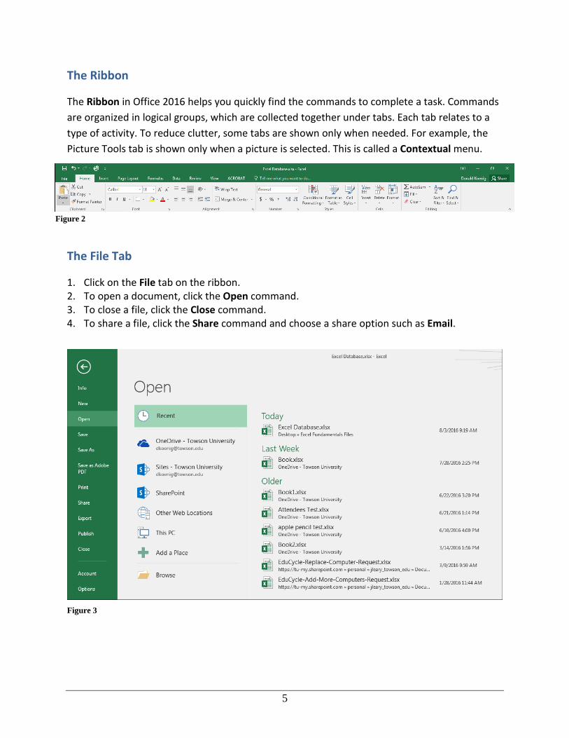
The Ribbon

The Ribbon in Office 2016 helps you quickly find the commands to complete a task. Commands are organized in logical groups, which are collected together under tabs. Each tab relates to a type of activity. To reduce clutter, some tabs are shown only when needed. For example, the Picture Tools tab is shown only when a picture is selected. This is called a Contextual menu.

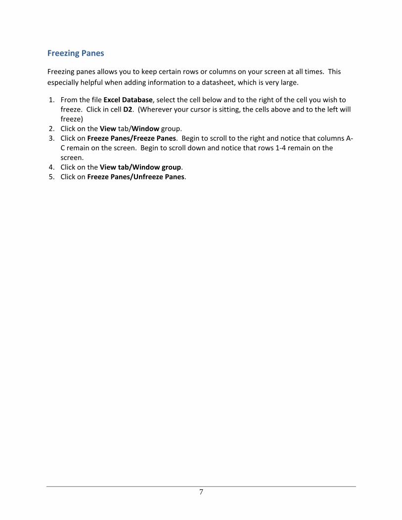
The File Tab

1. Click on the File tab on the ribbon. 2. To open a document, click the Open command. 3. To close a file, click the Close command. 4. To share a file, click the Share command and choose a share option such as Email.

Figure 2

Figure 3

6

Navigating in a File

Arrow Keys

Move one cell to the right, left, up or down

Tab Move once cell to the right Ctrl+Home To beginning file Ctrl+End To end of typed information

Home Beginning of a line End End Mode – Use arrow keys to navigate to the end of the data in any direction Page Down

Down one screen

Page Up Up one screen F5 Go To – Enter the cell you would like to select

Scroll bars Appear at the right and on the bottom of the screen. You may click the scroll arrows, drag the scroll box or click the scroll bar to move through the document.

Selection Techniques

You use selection in order to affect text, numbers or define a range to place in a formula. Workshop Activity - From within the document Excel Database, practice the following selection techniques:

Selecting an adjoining range of cells:

• Make sure your mouse takes the shape of a large white + sign. Drag your mouse across the range of cells.

• Click on the first cell in the range, hold down the SHIFT key on the keyboard and use your arrow keys to select the range.

• Click on the first cell in the range, hold down the SHIFT key on the keyboard and click on the last cell in the range.

Selecting non-adjoining cells

• Click on the first cell. Hold down your CTRL key on the keyboard. Click on other cells with the CTRL key held down.

7

Freezing Panes

Freezing panes allows you to keep certain rows or columns on your screen at all times. This especially helpful when adding information to a datasheet, which is very large.

1. From the file Excel Database, select the cell below and to the right of the cell you wish to freeze. Click in cell D2. (Wherever your cursor is sitting, the cells above and to the left will freeze)

2. Click on the View tab/Window group. 3. Click on Freeze Panes/Freeze Panes. Begin to scroll to the right and notice that columns A-

C remain on the screen. Begin to scroll down and notice that rows 1-4 remain on the screen.

4. Click on the View tab/Window group. 5. Click on Freeze Panes/Unfreeze Panes.

8

Creating a New Workbook

1. Click the File tab on the ribbon. 2. Click New. 3. In the New Workbook dialog box, select Blank Workbook. 4. Your new workbook will be presented on the screen.

Manage Worksheets

Working with Tabs

1. Click on the Insert Worksheet button at the bottom of the screen.

2. Double click on sheet 1 and type Totals and press ENTER. Add the following additional tabs:

a. Sheet 2 – January b. Sheet3 – February

3. Hold down your mouse button and drag the Totals tab after the February tab. 4. Right click on the Totals tab. 5. Move to Tab Color. Click on the color of your choice. 6. Recolor all other tabs using the same method. 7. Right-click on the February sheet. 8. Click on Delete. 9. Right-click on the January sheet and select Rename. 10. Type First Quarter.

Entering Data and Numbers

1. Click in cell A1 and type Monthly Budget. 2. Press ENTER or the down arrow on your keyboard to get to cell A4. 3. Go around the room and enter data that you may have in a monthly budget. Fill in both the

text and the amounts. Do not format the amounts. Examples are displayed.

Figure 5

Figure 4

9

Editing a Cell

1. Click in cell A1. 2. Press F2 on your keyboard. You know you are in edit mode because the mode indicator at

the bottom of the screen will say Edit. 3. Click after the word Monthly and press the BACKSPACE key to delete the word. Type

Quarterly and press ENTER. 4. Double click in cell A1. You know you are in edit mode because the mode indicator at the

bottom of the screen will say Edit. 5. Click before the word Quarterly and type your name. Click on the checkmark in the toolbar.

Notice this keeps you in the cell 6. Click in cell A1. Click in the Formula Bar. You know you are in edit mode because the mode

indicator at the bottom of the screen will say Edit. 7. Click after the word Budget. Press the SPACEBAR and type 2016 (or the current year) and

press ENTER. 8. Now on your own, click in cell A1. Get into edit mode using any of the above techniques.

Delete the current year and press ENTER.

Using the Autofill Handle

1. Select the cell B3 which contains the word January 2. Hover over the bottom right corner of the cell until a small black plus sign appears. 3. Click and drag the plus sign to the right two cells. Notice that the months February and

March appears. 4. Select B4:B8 5. Use the Autofill handle to drag the cells over to D8.

10

Creating Simple Formulas

All simple formulas begin with an = sign followed by the cell addresses to be added to the formula (Example: =A1+A2). To build a formula, use the following operators.

+ Addition - Subtraction * Multiplication / Division 1. In cell E3, type Totals.

2. Click in cell E4. This is where the formula will appear. 3. Begin your formula by typing a = sign. 4. Type b4 and then type +. Type c4 and then type +. Type d4 and then Press ENTER. Your

formula should be =b4+c4+d4. 5. Continue typing formulas in cells e5:e8 using the same technique. When you are finished,

your screen should appear similar to the one below. 6. Save the file to the Desktop as Quarterly Budget.

Figure 6

Figure 7

11

Formatting

Formatting Values

1. Select the ranges B4:D8. Click the Home tab/Number group. 2. Click Comma. Click the Decrease Decimal icon twice to show no decimal places. 3. Select the range E4:E8. Click the Home tab/Number group. Click the Currency icon. 4. In cell A2, enter todays date. 5. Click the Home tab/Number group. In the Format dropdown , select Long Date.

Using Fonts and Font Sizes

1. Press CTRL+HOME to get to cell A1. 2. In the Home tab/Font group. Click the dialog box launcher. 3. Click on the Font tab. Click on Century Schoolbook and 24 in the size box. 4. Click on OK. 5. Select the range B3:E3. Click the Home tab/Font group. Click the Font down arrow and

choose Century Schoolbook. 6. Click the Font Size down arrow and choose 14. Workshop Activity - Apply the same font size and style to the Budget Headings and Date.

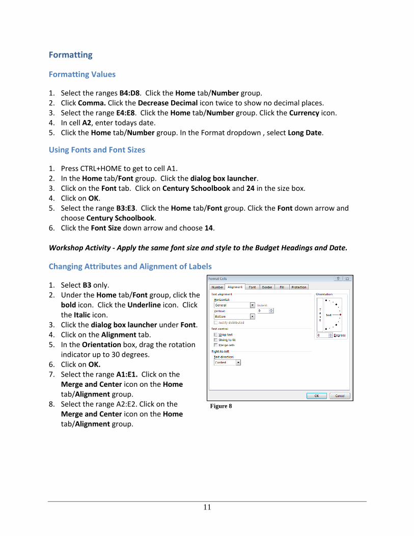
Changing Attributes and Alignment of Labels

1. Select B3 only. 2. Under the Home tab/Font group, click the

bold icon. Click the Underline icon. Click the Italic icon.

3. Click the dialog box launcher under Font. 4. Click on the Alignment tab. 5. In the Orientation box, drag the rotation

indicator up to 30 degrees. 6. Click on OK. 7. Select the range A1:E1. Click on the

Merge and Center icon on the Home tab/Alignment group.

8. Select the range A2:E2. Click on the Merge and Center icon on the Home tab/Alignment group.

Figure 8

12

Copying and Pasting Formats

1. Select cell B3. 2. Double-click on the Format Painter icon. (It looks like a paint brush) on the Home

tab/Clipboard group. 3. Click on cells C3-E3. 4. Click on the Format Painter again to turn it off.

Changing Column Widths

1. Select columns A:E. 2. From the Home tab/Cells group, click the Format down arrow. 3. Click AutoFit Column Width.

Alternatively, you can perform the following: 1. Place your mouse between the column headings until the mouse turns into a black arrow. 2. Double click the mouse or drag the mouse to the desired width.

Applying Colors

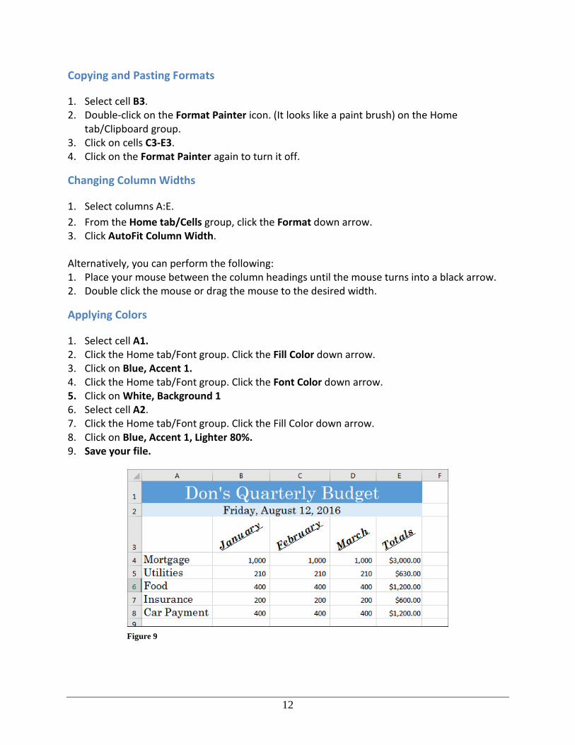
1. Select cell A1. 2. Click the Home tab/Font group. Click the Fill Color down arrow. 3. Click on Blue, Accent 1. 4. Click the Home tab/Font group. Click the Font Color down arrow. 5. Click on White, Background 1 6. Select cell A2. 7. Click the Home tab/Font group. Click the Fill Color down arrow. 8. Click on Blue, Accent 1, Lighter 80%. 9. Save your file.

Figure 9

13

Using Auto Calculate

(Navigate to the Excel 2016 Fundamentals Database)

1. Click on the Basic Calcs tab. 2. Select the range B5:B8. The Auto calculate function is located in the status bar. 3. Change the function to add Average, Count, etc. by right-clicking on the status bar.

Common Formulas

AutoSum Button

1. Click in cell E5. 2. Click on the Auto sum button in the Formulas tab. Press ENTER. 3. Continue to use the Auto sum button for cells E6:E8. Be careful with what it is selecting.

Workshop Activity - Autosum January:March columns of Quarter 1.

AutoSum Multiple Cells at Once

1. Select the range of B14:E18. 2. Click the AutoSum button to create totals for all cells all at once.

Figure 10

14

AVERAGE function using AutoSum Button

The AVERAGE function is a Statistical function which returns the arithmetic mean of a list of values. In other words, it adds up the total value of all the cells selected and divides it by the number of cells selected.

1. Click on the Average-Min-Max tab. 2. Click in cell G6. 3. Click the Formulas tab on the ribbon. 4. Click the down arrow underneath AutoSum and choose Average. 5. Press ENTER. 6. Click in cell G7. 7. Create another Average function. Notice it is trying to select the wrong area. Reselect the

correct area. 8. Drag the formula down to copy.

MAX function Using AutoSum Button

The MAX function returns the largest value of all the numbers evaluated by the formula.

1. Click in cell B18. 2. Click the Formulas tab on the ribbon. 3. Click the down arrow underneath AutoSum and choose Max. 4. Press ENTER. 5. Click in cell C18. 6. Create another Max. 7. Drag the formula across to copy.

MIN function using the AutoSum Button

The MIN function returns the smallest value of all the numbers evaluated by the formula.

1. Click in cell B19. 2. Click the Formulas tab on the ribbon. 3. Click the down arrow beside AutoSum and choose Min. 4. Press ENTER. 5. Drag the formula across to copy.

15

COUNT function using the AutoSum Button

The COUNT function counts the total number of cells that contain numbers.

1. Click the Count tab. 2. Click in cell L7. 3. Click the Formulas tab. 4. Click the AutoSum drop down arrow. 5. Click on Count Numbers. 6. Select from A4:A18. 7. Press Enter.

COUNTIF

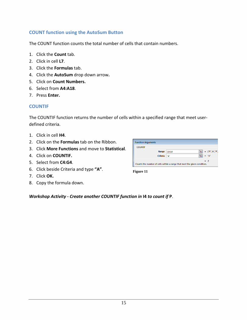
The COUNTIF function returns the number of cells within a specified range that meet user-defined criteria.

1. Click in cell H4. 2. Click on the Formulas tab on the Ribbon. 3. Click More Functions and move to Statistical. 4. Click on COUNTIF. 5. Select from C4:G4. 6. Click beside Criteria and type “A”. 7. Click OK. 8. Copy the formula down.

Workshop Activity - Create another COUNTIF function in I4 to count if P.

Figure 11

16

Sorting

The Sort command arranges worksheet data by text (e.g. A to Z and Z to A). You can use the Sorting & Filtering button to sort data by numbers, dates, times or color by more than 3 (and up to 64) levels. You may display more than 1000 items in the AutoFilter drop-down list, select multiple items to filter, and filter data in PivotTables. The new Sorting & Filtering button is located on the right side of the Home tab and on the Data tab on the Ribbon.

Setting up Data to Sort

Before you can sort data, make sure you set up the data correctly. There are a few rules you must follow:

• The column headings must be formatted differently than the data. For instance, the column headings are bold.

• The data below the column headings should be directly under the column headings. You should not skip a row for best results.

• The data within in each column must be formatted the same. For example, in the salary field below, all the numbers are formatted as currency.

Single Level Sort

1. Click on the Sorting and Filter tab. 2. Click anywhere in the Date Hired column. 3. Click on the Home tab on the ribbon. 4. Click on Sort & Filter in the Editing Group. 5. Click on Sort Oldest to Newest. 6. Go back and Sort Newest to Oldest.

Sort by multiple levels (up to 64)

1. Click in the Position field. 2. Click on Sort & Filter in the Editing Group. 3. Click on Custom Sort. 4. Choose Department beside Sort by. Choose A to Z as the Order. 5. Click on Add Level. 6. Choose Division beside Sort by. Choose A to Z as the Order. Workshop Activity - Practice sorting the following:

• Last Name (A-Z), First Name (A-Z) • Position (A-Z), Salary Largest to Smallest

17

Creating a Custom Sort Order

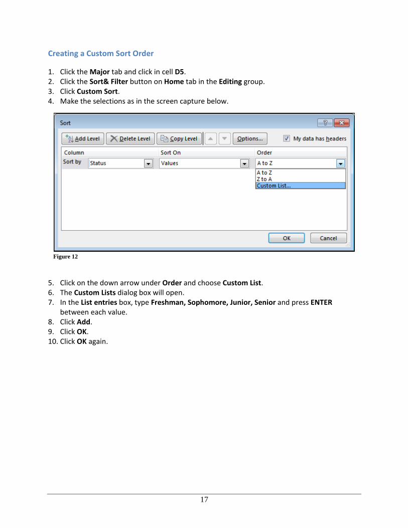
1. Click the Major tab and click in cell D5. 2. Click the Sort& Filter button on Home tab in the Editing group. 3. Click Custom Sort. 4. Make the selections as in the screen capture below.

5. Click on the down arrow under Order and choose Custom List. 6. The Custom Lists dialog box will open. 7. In the List entries box, type Freshman, Sophomore, Junior, Senior and press ENTER

between each value. 8. Click Add. 9. Click OK. 10. Click OK again.

Figure 12

18

Using AutoFilter

1. Click the AutoFormatting tab. 2. Click the Data tab on the Ribbon. 3. Click Filter in the Sort & Filter group. 4. Notice down pointing arrows will appear in each column heading. 5. Click the down arrow beside Position. A menu of options will appear. 6. Click Select All to deselect all items. 7. Click beside Group Mgr. and Office Manager. A check will appear in those boxes. 8. Click OK. All other data will be filtered out and only the data you selected appears.

Clearing a Filter

1. When a filter is applied, a small filter appears in the column heading. 2. Click the filter icon beside the Position field. A menu will appear. 3. Click Clear Filter From “Position”.

Workshop Activity - Practice performing the following filters:

• Department: Accounting • Clear the filter • Division: Fax • Clear the filter

Filtering on more than one Field

1. Filter by the Position field for find all Engineers. 2. Filter the Department field to find all Engineering. 3. Filter the Division field to find all Copier.

Clearing Multiple Filters all at once.

1. To clear the filter from multiple columns, click the Data tab on the Ribbon. 2. Click Clear from the Sort & Filter group.

Workshop Activity - Practice Performing the following multiple column filters:

1. Click the Major tab. 2. Select the data and turn on the filter. (Data/Filter)

• Filter by Status of Junior, Major of Business Administration. • Clear the filter. • Filter by Status of Senior, GPA of 3.50, 3.75 and 4.0 • Clear the Filter.

19

Creating an AutoFilter Using Criteria

You may create a custom filter using criteria. For example, you might create a filter that identifies all values greater than 500 or values less than 50.

1. Click the Sorting and Filtering tab. 2. Click the down arrow beside a number field such as Salary. A menu will appear. 3. Point to Number Filters and then click on the Greater Than… comparison operator. 4. The Custom AutoFilter dialog box will appear. Click in the white box beside the comparison

operator you have chosen and type 75000. 5. Click OK. 6. Be sure to clear your filter. Workshop Activity - Practice Performing the following multiple column filters:

1. Click the Tours tab. 2. Turn on the filter.

• Click the down arrow beside Number of Days. Click on Number filters and choose Less Than and type 14.

• Clear the filter. • Click the down arrow beside Number of Days. Click on Number filters and choose Less

Than or Equal To and type 14. • Clear the filter. • Click the down arrow beside Price. Click on Number filters and choose Top 10. • Choose Top 5 Items. • Clear the Filter. • Also practice above average and below average in the Price column. • Turn off the filter.

Filtering Data by Using Cell Attributes

If you have formatted a range of cells using a font color or fill color, you can filter on those attributes.

1. Click the Employee List tab. 2. Turn on the filter by clicking on Filter. 3. Click on the down arrow next to the Salary column. 4. Point to Filter by Color. A menu will appear. 5. Choose the color of Green. 6. Be sure to clear your filter.

Workshop Activity – Practice the following filters: • Filter the Last Name column by Red. Clear the filter. • Filter the Last Name column by Yellow. Clear the filter.

*Be sure to turn the filter off, by going to the Data tab and click on Filter.

20

Creating a Table to Sort and Filter

1. Click anywhere in the data. 2. From the Home tab/Styles group, click Format as

Table. 3. Select the Table Style Light 15 option. 4. Click OK in the Create Table window. 5. Notice the filter dropdown arrows have reappeared.

Changing the table Design

1. Click anywhere in the data. 2. Click the Design contextual tab. 3. Click the More button in the Table Styles group. 4. Experiment with the different styles.

Removing Duplicates

1. Select the Region Filter dropdown arrow 2. Filter by the Yellow duplicate color 3. Notice the duplicates. 4. Click the Design tab on the Ribbon. 5. Click Remove Duplicates in the Tools group. 6. Click OK and OK again. 7. Notice that 3 duplicates have been removed. 8. Clear the filter

Adding a Total Row

1. Click anywhere in the data. 2. Click the Design contextual tab. 3. Click Total Row in the Table Style Options group. 4. Move to row 83. Notice Total has been added. 5. Click in Salary total cell. Notice the dropdown arrow. 6. Click the down arrow and change the value to Average

Figure 13

21

Subtotaling Data

Data in a list can be summarized by inserting a subtotal. Before this can be done, you must first sort the list by the field you want the list subtotaled by.

Sorting Data for Subtotaling

Before creating a subtotal, you must sort your data on the field the subtotals will be based on.

1. Click the Subtotals worksheet. 2. Click in the Major Categories field. 3. Click the Data tab on the Ribbon. 4. In the Sort & Filter group, click on either Sort A to Z.

Subtotaling Data in a List

1. Click in the data you just sorted. 2. Click the Data tab on the Ribbon. 3. In the Outline group, click Subtotal. The Subtotal dialog box will appear. 4. Click on the down arrow beside At each change in: and choose the Department. 5. Under Use function, choose Sum. 6. Under Add subtotal to, click beside the Budget field. 7. Click OK. 8. Subtotals will be inserted at the end of each change in the column of sorted data.

Showing Levels

1. After creating a subtotal, notice the 1, 2, 3 in the upper left corner of the screen. 2. Click the 1 to view the Grand Total of the list. If there are pound sign symbols in the cell,

resize the column. 3. Click the 2 to view the Subtotals. 4. Click the 3 to view all the data. 5. You may also click on the collapse (-) button to the left of the summary rows. This will

collapse all the detail information. 6. Click the expand (+) button to left of the summary.

Removing Subtotals

1. Click the Data tab on the Ribbon. 2. Click Subtotal. The Subtotal dialog box will appear. 7. Click Remove All.