Embed Size (px)
Citation preview

Microsoft Excel XP
Intermediate
Jonathan Thomas
March 2006

Excel XP Intermediate Course
Contents
Lesson 1: Headers and Footers....................................................................................................1
Lesson 2: Inserting, Viewing and Deleting Cell Comments......................................................2 Options..................................................................................................................................................... 2
Lesson 3: Printing Comments......................................................................................................3
Lesson 4: Drawing ........................................................................................................................4
Lesson 5: Object Linked Embedding (OLE) .............................................................................5
Lesson 6: Lesson 6: Dynamic Data Exchange (DDE)................................................................5
Lesson 7: Working With Larger Spreadsheets..........................................................................6 Splitting the Window............................................................................................................................... 6 Removing the split from a window.......................................................................................................... 6 Freezing the headings .............................................................................................................................. 6 Freezing a row ......................................................................................................................................... 6 Freezing a column.................................................................................................................................... 6 Freezing a row and a column ................................................................................................................... 6
Lesson 8: Printing With Large Spreadsheets.............................................................................7 Printing part of the sheet .......................................................................................................................... 7 Print Titles................................................................................................................................................ 7
Lesson 9: Page Breaks ..................................................................................................................8 To Insert a break between rows ............................................................................................................... 8 To remove a specific page break between rows....................................................................................... 8 To remove a specific page break between columns................................................................................. 8 To remove all page breaks ....................................................................................................................... 8
Lesson 10: Joining text in different cells ....................................................................................8
Lesson 11: The "ISBLANK" Function and the "IF" Function ...............................................9 The "ISBLANK" Function ...................................................................................................................... 9 The "IF" Function .................................................................................................................................... 9 "IF" using calculations........................................................................................................................... 10
Lesson 12: View Options ............................................................................................................11
Lesson 13: Other Useful Options ..............................................................................................12 Tools, Options, Calculations.................................................................................................................. 12 Tools Options, Edit ................................................................................................................................ 12 Tools, Options, General ......................................................................................................................... 12 Tools, options, Custom lists................................................................................................................... 12
Lesson 14: Lists/Databases.........................................................................................................13 Filtering data .......................................................................................................................................... 13 Sorting data ............................................................................................................................................ 13
Lesson 15: Using Forms .............................................................................................................14

Excel XP Intermediate Course
Lesson 16: Linking......................................................................................................................15 Linking Worksheets............................................................................................................................... 15 Calculations ........................................................................................................................................... 15 Linking Workbooks............................................................................................................................... 15
Lesson 17: Consolidating Data ..................................................................................................16
Lesson 18: Setting Up Outlining................................................................................................17 Automatic outlining............................................................................................................................... 17 Manual outlining.................................................................................................................................... 17 Removing the outline............................................................................................................................. 17
Lesson 19: Using the Outline .....................................................................................................18 Collapsing the detail .............................................................................................................................. 18 Displaying or hiding the outline symbols.............................................................................................. 18 Levels of outline .................................................................................................................................... 18
Lesson 20: Subtotals ...................................................................................................................19 Adding subtotals .................................................................................................................................... 19 Subtotal levels........................................................................................................................................ 19 Options .................................................................................................................................................. 19 Removing subtotals ............................................................................................................................... 19


Excel XP Intermediate Course
Lesson 1: Headers and Footers
To set up or alter headers and footers select File, Page Setup and click on the Header/Footer tab.
The Header will appear at the top of the page, outside the page margins. The Footer will appear at the bottom of the page outside the page margins.
By default the page will have no Header and no Footer.
Click on the down arrow at the right hand side of the Header box to select from pre-setup Headers. Where there are more than one item, separated by commas, the left most item will be on the left hand side of the page, the next will be placed in the middle and the last on the right of the page.
Click on the one that shows what you want. If none are suitable you can create your own header. Click on the button:
You can now type in each section what you want to appear in that part of the Header. The buttons are for special situations
1

Excel XP Intermediate Course
The use of the special buttons
Brings up the Font dialogue box
Inserts the Page number (&Page)
Inserts the total number of pages (&Pages)
Inserts the date (&Date)
Inserts the time (&Time)
Inserts the Filename
Inserts the Sheet name (&Tab)
Inserts a picture
Note: The Footer works in an identical manner.
Lesson 2: Inserting, Viewing and Deleting Cell Comments
There are times when you wish to make comments about cells.
Adding
Highlight the cell to which you wish to add a note. Select Insert, Comment
A text box will appear which points to the relevant cell. Type the text in the box.
You will see a small red triangle at the top right-hand side of the cell, indicating that there is a note attached.
Options
By default you will see comment boxes overlaid on the spreadsheet. You can change this by selecting Tools, Options and clicking an option on the Comments line.
None means that you will see neither the boxes nor the red triangle indicator. Comment Indicator only will display the red triangle at all times and when you rest your
cursor on a cell with a comment the comment box will show Comment & Indicator is the default situation where both red triangle indicator and
comment box will be displayed at all times
Viewing
You can view each comment box by clicking on the or buttons on the Reviewing Toolbar. If you cannot see the Reviewing Toolbar select View, Toolbars, Reviewing. To see a comment on a particular cell you can rest the cursor over that cell and a yellow box will appear containing the relevant comment.
To see all the comments select View, Comment or click the Button on the Reviewing toolbar. Select either option again to hide all comments
Deleting
To delete a comment move to the relevant cell and select Edit, Clear, Comments or click the button on the Reviewing toolbar
2

Excel XP Intermediate Course
Lesson 3: Printing Comments
There are two ways of printing the cell comments. To select which of these you wish to use select File, Page Setup.
Click on the Sheet tab. You will see an option for Comments
Click on the down arrow
If you select At end of sheet when you print you will have an extra page on which the comments will be listed.
The comments are related to cells via the cell reference, so it would also be useful in this case to have the gridlines option and the Row and column headings option ticked.
This will mean that when the spreadsheet is printed the headings A, B, C etc will be shown across the top and 1, 2, 3 etc down the side.
If you select As displayed on the sheet the comment boxes will be printed as shown on the right. If however, you have chosen not to view some individual comment boxes then those will not be printed.
3

Excel XP Intermediate Course
Lesson 4: Drawing
Click on the icon from the toolbar to open a set of tools from which further icons can be selected:
In each case you will be required to click and drag in the spreadsheet to dictate a size for the shape. Once you have drawn the shape you can double click on it to alter various options.
For example, the arrow can be a variety of styles, widths or even colours:
If you draw an oval and double click on it you can choose not to fill it. you could then use it as a border for text
4

Excel XP Intermediate Course
Lesson 5: Object Linked Embedding (OLE)
You can embed an object (piece of information produced by a windows application) from another application within Excel. To edit the object thereafter merely double click on it and the original package will open. When you have edited it close the window and say Yes you wish to update the document.
To embed data both the applications must be open.
Open the package in which you wish to produce the object.
Highlight the area which you wish to import into Excel and select Edit, Copy
The area has now been copied to the clipboard.
Switch back to Excel, move the cursor where you want the object to appear and select Edit, Paste.
Lesson 6: Lesson 6: Dynamic Data Exchange (DDE)
The difference between embedding and a dynamic data link is that in embedding a copy of the original object becomes part of the document into which it is imported, and increases the size of the file quite heavily. With dynamic linking an image of the object is displayed in the file and it is linked to quite heavily. With dynamic linking an image of the object is displayed in the file and it is linked to the original.
Highlight and Copy your chosen text in the original application. Change to Excel, move the cursor to the cell in which you want the text to appear and select Edit, Paste Special.
In the Window which appears, make sure that the Paste Link option has been selected.
Note: To insert text from Word into a cell you must also click on text. If you do not do this the text will be placed in a box over the spreadsheet.
Any changes made to the original document will be reflected in Excel.
If you have linked from another spreadsheet and wish to break the link, highlight the cell(s), select Edit, Copy, then select Edit, Paste Special, Values, OK
You cannot make a link from Word into a text box
If you are having trouble with updating information, or are getting an errror message saying that an application cannot update information it should be collecting from Excel you should check in Tools, Options General to see that the Ignore other applications is not ticked.
5

Excel XP Intermediate Course
Lesson 7: Working With Larger Spreadsheets
Splitting the Window
You may wish to see two parts of your spreadsheet at the same time. This can be done by splitting the window.
Horizontally Move the cursor to the right-hand side of the screen, above the scroll up arrow, as shown. Click the mouse whilst dragging the cursor down to the correct position.
Vertically
Move cursor to the bottom right of the screen, to the right of scroll right arrow, as shown. Click the mouse whilst dragging the cursor down to the correct position.
Horizontally and Vertically Place your cursor in the cell above which, and to the right of which you wish the window to split. Selelct Window, Split
Removing the split from a window
Double click on the relevant bar to remove an individual bar.
Select Window, Remove split to remove all splits
Freezing the headings
If you have a lot of data underneath headings you may wish to split the window so that you can see the headings at all times. To do this you will need to freeze the row and/or column containing the headings as given below
Freezing a row
Highlight the row below the row you wish to freeze by clicking on the row number to the left hand side of the screen. Select Windows, Freeze panes.
Freezing a column
Select the column to the right of the column you wish to freeze by clicking on the column letter to the top of the spreadsheet, then select Windows, Freeze panes.
Freezing a row and a column
Highlight a single cell to the right and below the row and columns you wish to freeze, then select Windows, Freeze panes.
To remove the Split and frozen panes
Select Window, Remove Split (Or Window, Unfreeze Panes)
6

Excel XP Intermediate Course
Lesson 8: Printing With Large Spreadsheets
Printing part of the sheet
You may wish to print a certain part of your database on a regular basis. To do this you must first set the Print Area
Select File, Page Set-up and click on the Sheet option.
Clicking in the Print Area box then click and drag over the area of the spreadsheet.
If you need to see beneath the dialogue box, click on the button
The dialogue box will shrink to show only the required box
Click on the button to return to the full dialogue box.
When you click and drag in the spreadsheet the relevant range will be built up in the Print Area box. You can select more than one area by separating them with a comma. These areas will print on separate sheets of paper
You can also highlight the area you wish to print, select File, Print Area and Set Print Area.
Print Titles
If you are printing a spreadsheet which goes across several pages you may wish to repeat the headings at the top and left of your table on each page.
Select File, Page Setup, Sheet and click in the Rows to repeat at top box
Click on the spreadsheet to select a row (or adjacent rows). Use the button to hide the dialogue box as before. When you have selected the row click on the
Repeat for Columns to repeat at left
7

Excel XP Intermediate Course
Lesson 9: Page Breaks
To Insert a break between rows
Highlight the row below the point at which the new page will start. Select Insert, Page Break. To Insert a break between columns Highlight the column to the right of the point at which the new page will start. Select Insert, Page Break. To remove a specific page break between rows
Highlight the row below the page break. Select Insert, Remove Page Break. To remove a specific page break between columns
Highlight the column to the right of the page break. Select Insert, Remove Page Break. To remove all page breaks
Highlight the whole document and select Insert, Remove page breaks Note to highlight the whole document you can click on the blank button at the top left
Lesson 10: Joining text in different cells
You may have text in different cells which you wish to combine.
In the example shown right we may wish to create a third column which shows the name as a whole e.g. Elaine Yates
We can use the & operator to join text as shown below
=B2 & A2
This would result in ElaineBates which is obviously missing a space between the words, so we need to ensure that we add the space too as shown below (note that there is a space between the " marks)
=B2 &" " & A2
This will result in Elaine Bates which looks much better!
We could expand this. Look at the example shown right.
Supposing we want to be able to say
"Ms Elaine Bates obtained a Fail in Maths"
We could use the formula:
=C2&" "& B2 &" " & A2 " obtained a " & D2 & " in " D1
Note that we have added a space between B2 and A2. Note too that there should be a space before and after any text inside quotes!
8
Excel XP Intermediate Course
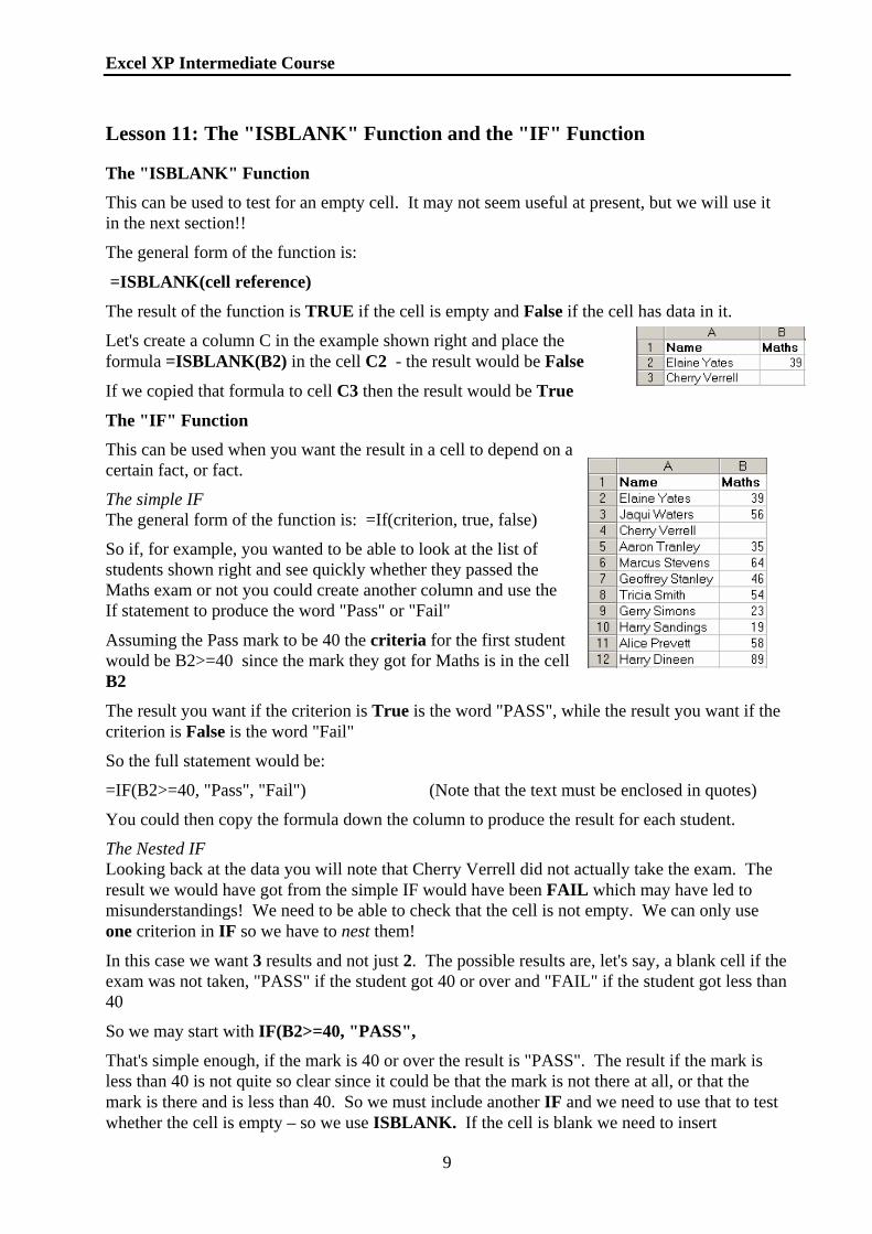
Lesson 11: The "ISBLANK" Function and the "IF" Function
The "ISBLANK" Function
This can be used to test for an empty cell. It may not seem useful at present, but we will use it in the next section!!
The general form of the function is:
=ISBLANK(cell reference)
The result of the function is TRUE if the cell is empty and False if the cell has data in it.
Let's create a column C in the example shown right and place the formula =ISBLANK(B2) in the cell C2 - the result would be False
If we copied that formula to cell C3 then the result would be True
The "IF" Function
This can be used when you want the result in a cell to depend on a certain fact, or fact.
The simple IF The general form of the function is: =If(criterion, true, false)
So if, for example, you wanted to be able to look at the list of students shown right and see quickly whether they passed the Maths exam or not you could create another column and use the If statement to produce the word "Pass" or "Fail"
Assuming the Pass mark to be 40 the criteria for the first student would be B2>=40 since the mark they got for Maths is in the cell B2
The result you want if the criterion is True is the word "PASS", while the result you want if the criterion is False is the word "Fail"
So the full statement would be:
=IF(B2>=40, "Pass", "Fail") (Note that the text must be enclosed in quotes)
You could then copy the formula down the column to produce the result for each student.
The Nested IF Looking back at the data you will note that Cherry Verrell did not actually take the exam. The result we would have got from the simple IF would have been FAIL which may have led to misunderstandings! We need to be able to check that the cell is not empty. We can only use one criterion in IF so we have to nest them!
In this case we want 3 results and not just 2. The possible results are, let's say, a blank cell if the exam was not taken, "PASS" if the student got 40 or over and "FAIL" if the student got less than 40
So we may start with IF(B2>=40, "PASS",
That's simple enough, if the mark is 40 or over the result is "PASS". The result if the mark is less than 40 is not quite so clear since it could be that the mark is not there at all, or that the mark is there and is less than 40. So we must include another IF and we need to use that to test whether the cell is empty – so we use ISBLANK. If the cell is blank we need to insert
9

Excel XP Intermediate Course
"nothing" which we do by putting "" with nothing between the quotes. If the cell is not blank it means that the student has taken the exam and got less than 40 – so we need "FAIL". The whole IF statement is then:
i.e. IF(B2>=40, "PASS", IF(ISBLANK(B2), "", "FAIL")
You can nest up to 7 If statements
For example, supposing you wanted to calculate Grades from the marks as shown below:
Mark range Grade 0-40 Fail 41-60 E 61-70 D 71-80 C 81-90 B 91-100 A
The IF statement would be:
=IF(B2<=40,"Fail",IF(B2<=60,"E",IF(B2<=70,"D",If(B2<=80,"C", IF(B2<=90,"B", "A")
There that's one for you to think about!
Note that we start with the lowest first! Let's consider what would happen if we started with the highest grade first
e.g. =IF(B2>90, "A", IF(B2>80, "B", IF(B2>70, "C)…..
Let's say B2 has the number 94 in it. The first criterion (B2>90) is True, so the grade given is A, But the second criterion (B2>80) is also True so the grade given is now B and so on!
"IF" using calculations
You can also use formulae in the True and/or False section.
e.g. using the example shown right, note that the cost of the item depends on whether it is VAT rated or not.
To work out the cost, assuming a VAT rate of 17.5%, we could use the formula below in cell D2
IF(B2="yes", C2*1.175, C2)
Note that if the item is VAT rated a calculation is carried out, while if it is not VAT rated the price is copied into the Cost column.
10

Excel XP Intermediate Course
Lesson 12: View Options
There are many things you can change about the way Excel displays things. To so this go to Tools, Options
Choose whether to show the Formula Bar at the top of the window, or the status bar at the bottom.
Set options for Comments
Choose whether to see objects, such as charts, pictures, circles, text boxes etc which are overlaying your sheet. If you choose Show Placeholders you will see empty boxes where some types of objects are. This means that
you do not forget that there are objects there, but the screen is updated quicker, when moving around, than it would be if it had to redraw the details of the object each time.
Under the Window options area you can choose whether to view various things:
Formulas gives you the option of viewing in the cell the formula rather than the result of the formula. If you have the formulae showing and you print the spreadsheet then the formulae themselves will be printed. This gives you the opportunity to check the formulae at leisure.
Gridlines give you the option of not seeing the gridlines on screen (the option for printing is under File, Page setup, sheet)
Row and column headers: This refers to Excel’s own row and column headers. i.e. A, B, C… and 1, 2, 3….. This is useful if you have chosen to print formulae. You can then relate the cells defined in the formulae to the sheet more easily.
Outline symbols will be covered later
Zero values allows you to define whether you wish to see zero or merely have a blank cell
Sheet tabs: It may be that you have several sheets containg calculations, but only one sheet on which you wish users to enter data. You could hie the sheet tabs so that users are not aware that there are any other sheets than the one they can see.
11

Excel XP Intermediate Course
Lesson 13: Other Useful Options
There are many options, below are some of the most commonly useful:
Tools, Options, Calculations
Precision as displayed: Often you will format the result of a calculation to show to a set number of decimal places, for example. If you use that result in another calculation the number used by default is the actual value, not the formatted one. E.g. the answer to a formula may be 6.6666667 and you format it to 6.67, but 6.6666667 would be used if this cell was involved in any other formula. This can result in being a penny or so out in monetary calculations! If you click on precision as displayed then if you see 6.67 then that value will be used in any other calculation.
Tools Options, Edit
Edit directly in cell: You can normally edit a cell by double clicking in it. If you remove this option you will only be able to edit a cell by clicking on the formula bar.
Allow cell drag and drop: If you have a habit of accidentally dragging and dropping you may find it useful to remove this option
Move selection after enter: you can control whether the selection moves to another cell after you have pressed the enter key, and if so in which direction it should move.
Fixed decimal places: If you are consistently typing numbers with the same number of decimal places you can set this option. E.g. If you fix 2 decimal places then you can type 3400 for 34.00, or 34 for 0.34. Note that this will apply to every value you type until you remove the option.
Tools, Options, General
Recently used file list: This defines how many recently used files will be listed at the bottom of your File menu so that you can open them quickly.
Sheets in new workbook: This defines how many sheets each new workbook (file) will have.
Default file location: This allows you to define a folder into which the File, Open and File, Save As dialogue boxes will take you
Tools, options, Custom lists
You can use this to set up your own lists. For example, to create a list for Qtr1, Qtr2, Qtr3 and Qtr 4 click on NEW LIST in the Custom List box.
In the List entries box type Qtr1 and press Enter. On the next line type Qtr2 and so on. Once you have completed the list click on the button.
You can now type Qtr1 in a cell in your sheet, select the cell and click on the small square on the bottom right of the selection box to drag down (or to the right) to create the full list, repeated for as long as you drag the box
12

Excel XP Intermediate Course
Lesson 14: Lists/Databases
A list comprises of columns representing fields and rows which represent the records. The first row in this list must contain the field names. The data in this list can be treated like a database which can be filtered and sorted and to which search criteria can be applied from within a Form.
Filtering data
A filter allows only those rows of data to show which meet a specified criteria. The auto-filter command applies drop-down arrows so you can choose the item to display, and Excel hides the rows which are not chosen. To choose a criteria, position the cursor within any cell containing a heading in the list, select Data, Filter, Auto-Filter. A list of each different entry contained within the selected column will appear. If you wish to find rows with a particular value you can click on one of these values and all relevant rows will be shown. Other rows are hidden.
Click on the drop-down arrow at the top of the required column and choose Custom. From the dialogue box which appears, select an operand (=, >, <, etc) and enter the value or text to compare with. Click on OK to action the command.
To show all records/rows again, either Click on the drop-down arrow for the relevant column and select All or select Data, Filter, Show All to clear the criteria from all the columns
Sorting data
Highlight the column or row which is to be sorted and select Data, Sort.
All columns neighbouring the highlighted one will now be selected since you must not sort only one column without taking related data, and the Header Row option will be marked to show that your list contains titles (these should not be highlighted, however since you do not wish to sort these). The title for the column which was chosen to be sorted will appear in the Sort by. Any further rows or columns which are needed for sorting can be added - up to a total of three.
13

Excel XP Intermediate Course
Lesson 15: Using Forms
It is possible to enter and query the list data using a data form.
Entering Data
Position the cursor within the list. If there is no data yet you should click on one of the headings. Select Data, Form. This will create a form displaying the boxes for the first record in the list. The command buttons on the right hand side of the form allow navigation through the data.
Note: in the form on the right the columns for Price and Quantity require data to be typed in, whereas the Cost column is calculated via a formula
takes you directly to a new row removes the data being viewed and moves
row form below to take its place (effectively it deletes the cells)
scraps changes you have made to a particular row of data. It can only be used while you are still viewing that row
moves you to the previous row of data
moves you to the next row of data Searching for Data
Click on this button to search for a particular “record” or row of data. The box will change as shown on the right. Note that the Criteria button has now become the Form button, allowing you to return to the form. Also the Delete button has become the Clear button which allows you to remove all criteria from the boxes Type the criteria you require. To see data which meets these requirements click on the Find Next or Find Prev button. You will then return to the form and can continue clicking on Find Next or Find Previous. Click on the Criteria button to return to that screen
14

Excel XP Intermediate Course
Lesson 16: Linking
Linking Worksheets
To add headings to all sheets at once, for example, click on one sheet which you want to use, and then hold the Ctrl key down while you click on any others. (or hold the Shift key down and click on the last sheet in the list which you wish to group)
The grouped tabs will turn white. e.g. In the illustration below qtr 1, qtr 2 and qtr 3 are grouped and anything added to one of them will be added to all.
Calculations
You can do calculations using cells from other sheets by defining the sheet name, followed by the cell reference. e.g. ‘Qtr 1’!B1+’Qtr 2’!B1+Year!B1 While this can be typed in it is often easier to start by typing the = sign in the cell in which you want the answer to appear and then change to the relevant sheet and click on the required cell. You can then type an operator (e.g. +), change to another sheet and click on the required cell. In this way Excel will build up the cell definitions for you correctly. Press Enter when the formula is complete. Note
1. Where a sheet name contains spaces it must be enclosed in single quote marks 2. An exclamation point must always follow the sheet name
Linking Workbooks
It is also possible to create links to cells in other workbooks. In this case the link description is made up of:
The location on disk of the workbook The worksheet name within the workbook The cell reference within the worksheet
e.g. ='C:\spreadsheets\[EXAM.XLS]EXAM'!$B$24
Again, you will find it easier to allow Excel to build up the description for you. Make sure you have all necessary files open, type the = sign in the cell in which you want the answer to appear and then click on Window and the file name, click on the cell, type an operator and continue until the formula is complete. Then press the Enter key. Note
1. Quotes are must be placed around the full workbook / worksheet name
2. If the file only has one sheet then the sheet name will be omitted 3. While both files are open the full path will probably not be displayed
15

Excel XP Intermediate Course
Lesson 17: Consolidating Data
To quickly produce summary totals etc. for several sheets which are set out in the same way, move to the sheet on which you wish the summary figures to appear, highlight the range of cells which relates to the total number of cells on the other sheets which you want to consolidate and select Data, Consolidate
1. The dialogue box on the right will appear. Select the required function from the Function box. 2. Click in the Reference box and click on the first sheet tab to be summarised, highlight the relevant area (this usually matches the area which you chose to put the answers in) 3. Click on the Add button. That reference will be shown in the All References box.
4. Click on the next sheet tab to be summarised and repeat steps 2 and 3. Repeat until you have defined all the sheets to be summarised and then click the OK button.
Note
If figures are changed on the original sheets the consolidated total will not automatically change. You will need to highlight the cells and select Data, Consolidate, OK
To ensure that the consolidated totals do change, click on the Create links to source data option. This creates an outline, which will be covered in the next 2 tasks, with hidden rows containing links to the raw data.
16

Excel XP Intermediate Course
Lesson 18: Setting Up Outlining
Often the spreadsheet contains raw data which is summarised in various ways. Usually you really only want to see the summarised data as your finished product. The outlining of a sheet allows only the summarised data, totals etc, to be viewed.
Using the outline tools you can group rows (or columns) together. Once you have done this you will see symbols in the left margin which will enable you to view the details of the group or not as you wish.
Data before outlining with totals
Data after outlining with all data shown
Data after outlining with only totals shown
Notice that the missing rows are hidden. The row numbers are missing
Automatic outlining
Place your cursor somewhere in the relevant data and select Data, Group and Outline, Auto Outline. Excel searches for totals, etc., and groups the rows above them. You will see symbols to the left of totals with lines going from these up past rows used to produce the total.
Manual outlining
To set up the same thing manually, select rows 1 to 3, in the example on the left above, and select Data, Group and Outline, Group (If you have not selected the complete rows you will be asked whether you wish to group rows or columns.) You will then see to the left of the total row. Repeat this individually for rows 7 to 8 and 10 to 12. You can also use the shortcut keys Alt, Shift, to group rows or columns once you have selected them.
Ungrouping
To ungroup select the relevant rows or columns and press Alt, Shift
Removing the outline
To remove the whole outline select Data, Group and Outline, Clear Outline
17

Excel XP Intermediate Course
Lesson 19: Using the Outline
Once you have set up the outline you can use it to view the data in different ways
Collapsing the detail
To see only the rows containing totals, select all the data and select Data, Group and Outline, Hide detail. Alternatively, click on the button at the left of each total to hide the details for that total. The Banana and Pears Totals on the right have been collapsed
Viewing the detail
To see the rows that are used to produce the total, select all the data and select Data, Group and Outline, Show detail
Alternatively, click on the button at the left of the relevant total. This has been done in the case of Apples above.
Displaying or hiding the outline symbols
Select Tools, Options, View and remove the tick from Outline symbols. You can also do this by pressing Ctrl 8. Note that the outline still exists. Press Ctrl 8 to view the symbols again.
Levels of outline
You can create up to 8 levels of outline. The example on the right has 4 levels. The lowest level, 4, is all the data. Level 3 is the monthly totals, level 2 the Fruit totals and level 1 the Grand total. At the top of the outline symbols area you can see numbers Representing these levels. If you click on the button you will see only the Grand total If you click on the button you will see all totals down to Fruit totals andso on down to the button which will show all the details When creating an outline manually it is important to start creating the lowest level groups first.
Notes: 1. To produce a chart using only the totals, start with the outline collapsed to the level you wish to plot and after
producing the chart ensure that under Tools, Options, Chart the option Plot visible cells only is ticked.
2. In some cases, if you remove an outline or ungroup while showing only subtotals, i.e. there are hidden rows, the rows remain hidden even after the outline is removed. Use the shortcut keys ‘Ctrl Shift (’ to unhide selected rows and ‘Ctrl Shift )’ to unhide selected columns (Ctrl 9 hides rows and Ctrl 0 hides columns)
3. All that we have done with rows applies equally well if your totals are across columns, In this case the outline symbols will be across the top of the spreadsheet.
18

Excel XP Intermediate Course
Lesson 20: Subtotals
If you have lists of data which is laid out in columns, you can quickly produce subtotals. You would first need to sort the data so that it is grouped as you wish the subtotals to be created. Adding subtotals
Place your cursor somewhere in the list of data and select Data, Subtotals
You then need to select from the At each change in box the column which you wish to define how the subtotals are calculated
From the Use function box you can chose what kind of calcualtion to use, e.g. SUM, AVERAGE etc.. Note that you can only use one function across all the subtotals
In the Add Subtotal to box tick the boxes for totals which you wish to add
Click OK
Subtotal levels
If you wish to have subtotals within subtotals, e.g. in our example you could have monthly totals inside the Fruit totals, you must start by inserting the subtotals for the highest level, e.g. Fruit and then when you have those subtotals you do the process again for the next level, e.g. Month, but when doing this second level you must remember to remove the tick from Replace current subtotals or you will lose the first level totals. (This prcess is often referred to as ‘nesting’)
Options
If you remove the tick from Summary below data the Grand total will be placed at the top of the data and the subtotals above their groups
If you add a tick to Page break between groups then each group will be placed on a separate page
Removing subtotals
Click in the data and select Data, Subtotals then click on the button. This will remove all levels of subtotals.
19


![Manual Excel Xp[1]](https://img.pdfslide.net/doc/110x75/5571f3d449795947648ea407/manual-excel-xp1.jpg)