Embed Size (px)
Citation preview
Migration, Production Structure and ExportsSome New Evidence from Italy
Giuseppe De Arcangelis∗ Edoardo Di Porto† Gianluca Santoni‡
December, 2012
(preliminary and incomplete)
Abstract
In this paper we study the effect of migration in a two-sector model where productionis performed with one freely mobile factor and sector-specific CES composites of laborservices. Factor demands in the two sectors are specified in terms of labor servicesand they differ since the the two types of labor services have different productivitiesto achieve the two tasks. While the freely mobile factor is inelastically supplied and isgiven within the geographical area that we consider, individuals supply labor servicesto serve two different types of tasks – simple and complex tasks. Migrants and nativesdiffer in terms of productivity in performing the different tasks. The model shows thatan inflow of migrants has an effect on the production structure in favor of the sector thatneeds more intensively simple tasks, like manufacturing, in the spirit of the Rybczynskieffect. In this version of the model the owners of the freely mobile factor gains fromimmigration since the remuneration of the mobile factor inequivocably rises in nominaland real terms.
We take advantage of a detailed data set of migrants’ work permits at the provinciallevel (NUTS3) in Italy to assess the effect of migrants’ inflows on the production andexport structure of the Italian provinces. By assuming that the service sector is relativelymore intensive in complex rather than simple tasks with respect to the manufacturingsector, our theoretical model is confirmed by the data. We find that in provinces rela-tively more endowed with migrants the production structure is characterized by a lowerservices-to-manufacturing ratio in value-added terms. The same pattern is confirmed inthe export structure. Nationality concentration seems also to play a role
Keywords: International Migration, International Trade.JEL Classification Codes: F22, C25.
∗Dipartimento di Scienze Sociali ed Economiche, Sapienza University of Rome; e-mail:[email protected].†Dipartimento di Economia e Diritto, Sapienza University of Rome; e-mail:
[email protected].‡Manlio Masi Foundation - Italian Institute for Foreign Trade; e-mail: [email protected].
1
1 Introduction
The effect of immigration on the production and export structure of an economy is a highlydebated topic. In the traditional Rybczynski framework, a relative increase in the productionfactor embodied in the migration inflow will bias the production structure towards sectorsthat more intensively use the increased factor. Indeed, although young and well-educated,legal migrants are usually employed in low-skill positions and are paid less than natives. So,inflows of new migrants usually lower low-skilled wages and favor industries that use relativelymore unskilled workers (see for instance Gandal, et al., 2004). In a more dynamic framework,by taking advantage of cheaper effective labor, domestic industries have a strong incentive todelay restructuring and to lag behind in the switch towards more labor-saving technologies.
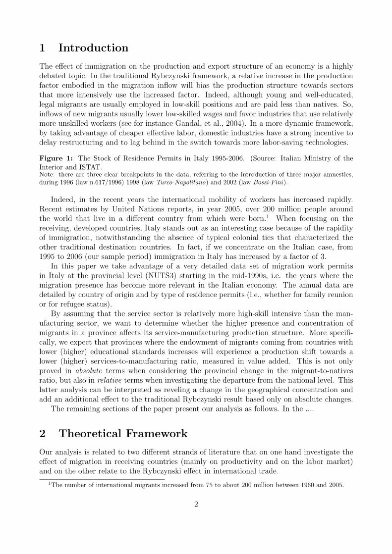
Figure 1: The Stock of Residence Permits in Italy 1995-2006. (Source: Italian Ministry of theInterior and ISTAT.Note: there are three clear breakpoints in the data, referring to the introduction of three major amnesties,during 1996 (law n.617/1996) 1998 (law Turco-Napolitano) and 2002 (law Bossi-Fini).
Indeed, in the recent years the international mobility of workers has increased rapidly.Recent estimates by United Nations reports, in year 2005, over 200 million people aroundthe world that live in a different country from which were born.1 When focusing on thereceiving, developed countries, Italy stands out as an interesting case because of the rapidityof immigration, notwithstanding the absence of typical colonial ties that characterized theother traditional destination countries. In fact, if we concentrate on the Italian case, from1995 to 2006 (our sample period) immigration in Italy has increased by a factor of 3.
In this paper we take advantage of a very detailed data set of migration work permitsin Italy at the provincial level (NUTS3) starting in the mid-1990s, i.e. the years where themigration presence has become more relevant in the Italian economy. The annual data aredetailed by country of origin and by type of residence permits (i.e., whether for family reunionor for refugee status).
By assuming that the service sector is relatively more high-skill intensive than the man-ufacturing sector, we want to determine whether the higher presence and concentration ofmigrants in a province affects its service-manufacturing production structure. More specifi-cally, we expect that provinces where the endowment of migrants coming from countries withlower (higher) educational standards increases will experience a production shift towards alower (higher) services-to-manufacturing ratio, measured in value added. This is not onlyproved in absolute terms when considering the provincial change in the migrant-to-nativesratio, but also in relative terms when investigating the departure from the national level. Thislatter analysis can be interpreted as reveling a change in the geographical concentration andadd an additional effect to the traditional Rybczynski result based only on absolute changes.
The remaining sections of the paper present our analysis as follows. In the ....
2 Theoretical Framework
Our analysis is related to two different strands of literature that on one hand investigate theeffect of migration in receiving countries (mainly on productivity and on the labor market)and on the other relate to the Rybczynski effect in international trade.
1The number of international migrants increased from 75 to about 200 million between 1960 and 2005.
2
The literature on the effects of migration in receiving countries has mainly investigatedlabor market effects, in particular effects on wages. There is a general consensus that thecompetition of migrants is more intense only in some segments of domestic labor markets,typically the lower end in terms of education attainment. Borjas (2003) and Card (2001and 2007) have debated this issue with different geographical perspectives. Ottaviano andPeri (2012) give a different perspectives by assuming competition in all segments, but withimperfect substitutability.
Peri and Sparber (2009) take an original approach borrowing from the recent literature oninternational trade in task and offshoring (see, for instance, Grossman and Rossi-Hansberg,2008). They highlight the importance of labor services rather than workers and consider thecase of a labor supply composed by heterogeneous workers in terms of labor services that areeither natives or foreign-born. D’Amuri, et al. (2010, 2012) apply this same methodology tosome European countries.
In our model we extend this approach to a two-sector framework and we want to highlightthe production effects rather than the wage effect of new immigration flows. According tothe traditional theories of international trade, the production effects of an increase in factorendowments is described by the Rybczynski effect. Previous studies that related this effectto migration are Hanson and Slaughter (2002, 2004) when considering the local effect in theUS states or in the particular case of Israel (inflow of highly-educated migrants from Russiaat the end of the 1980’s). These studies have given an important contribution by means of asimple accounting model and with simulation exercises, but without an estimated model.
Let us consider two sectors, manufacturing (M) and services (V ), and assume that the twoproduction functions are well-behaved Cobb-Douglas:
Yj = AjH(1−α)j Nα
j
Output Yj in each sector j = M,V is produced with two different inputs: (a) the factorH, which is freely mobile between the two sectors, and (b) the specific factor Nj, which ischaracterized by a sector-specific composition of labor services. The setup is similar to theRicardo-Viner specific-factor model (see Jones, 1971, or Feenstra, 2004, p.72). The elasticityof output to the mobile factor H is the same; the two sectors differ because of the TFPparameter Aj and the different composition of the factor Nj as discussed below.2
The mobile factor H can be traditionally interpreted as capital, but it can be any type ofproduction factor that is in fixed supply in our market (being the province in our case), butthat can be used by both sectors, i.e. land, a general type of labor, public services, etc.3
The demand for H in each sector is given by its marginal productivity:
∂Yj∂Hj
= α
(Nj
Hj
)1−α
Given the sector mobility, arbitrage implies that the nominal remuneration of H be equalin the two sectors; hence:
2This simplifying assumption could be easily released, but at the cost of a more cumbersome algebra.3Peri and Sparber (2009) consider a CES production function in one-sector model where one of the two
intermediate services corresponds to the amount of high education workers and functions as a sort specificfactor.
3
αpM
(NM
HM
)1−α= αpV
(NV
HV
)1−α
or:
(HM
HV
)=
(pMpV
) 11−α NM
NV
As a consequence, the relative production is simply a function of the relative output priceand the relative specific-factors supply:
YMYV
=
(pMpV
) α1−α NM
NV
(1)
Let us assume for now that the relative price is fixed since, for instance, it is given fromabroad (we assume a small-open province or region or economy).
Let us name WH the nominal “wage” of the mobile factor H, and Wj for j = M,V thenominal “wages” of the two specific factors, respectively Nj, j = M,V . From the Cobb-Douglas characteristics:
pj = AWαHW
1−αj
for j = M,V , where A ≡[(
α1−α)1−α
+(
α1−α)−α]
.
It is then well-known:
WM
WV
=
(pMpV
) 11−α
(2)
Hence, a given relative output price implies a given relative “wage” index of the specificfactors.
Another important consequence of (1) (and given relative prices) is that the dynamics ofrelative output is fully determined by the relative quantity of the two specific factors, whichare composite indexes of labor services or labor tasks.
The composite factor Nj is a sector-specific input because of its composition in terms oflabor services. We consider two different types of labor services: “simple” manual tasks (S)and “complex” (abstract, communication intensive) tasks (C). The labor services are thencombined differently in the two sectors via a CES aggregation as follows:
Nj =[βjS
σ−1σ
j + (1− βj)Cσ−1σ
j
] σσ−1
(3)
where the coefficient βj represents the relative productivity of “simple” tasks to “complex”tasks and we assume that simple tasks S are relatively more productive in the M sector, i.e.βM > βV . The elasticity of substitution between tasks is equal to σ and does not changebetween the two sectors.
Then:
NM
NV
=
[βMS
σ−1σ
M + (1− βM)Cσ−1σ
M
βV Sσ−1σ
V + (1− βV )Cσ−1σ
V
] σσ−1
=
4
=SMSV
[βM + (1− βM)c
σ−1σ
M
βV + (1− βV )cσ−1σ
V
] σσ−1
(4)
where cJ ≡ CjSj
for j = M,V .
Equation (4) shows that the relative quantity of the two specific factors depends on thetwo ratios cM and cV , and on the ratio SM
SV. Ultimately, also relative output depends on the
same three ratios.
Roadmap
We recall that labor services could “travel” between the two sectors and there exists onesingle market for complex tasks and one single market for simple tasks for the whole economy.The quantity of each specific labor composite – i.e. NM and NV – is determined by the demandfor each labor service from each sector and by the wage.
As shown below, the relative price of labor services is linked to the relative wage indexesin the two sectors and, ultimately, by the relative price of output. As cleared up below, therelative demand for labor services in each sector depends only on the relative wage. Whenthe relative wage is given (as in our case because we assume given relative output price), thenthe relative supply of labor services is given as well as the relative demand of labor servicesfrom each sector. The only variable to determine is the relative weight of each sector, whichmeans the ratio SM
SVand therefore the output ratio. Then any exercise of comparative statics
will have an effect on the relative output ratio.
2.1 The relative wage of tasks
From the CES characteristics, the “wage” of each composite factor is the following:
Wj =[βjW
1−σS + (1− βj)W 1−σ
C
] 11−σ
for j = M,V . Let us define ω ≡ WC
WS. So:
WM
WV
=
[βM + (1− βM)ω1−σ
βV + (1− βV )ω1−σ
] 11−σ
Let us define W ≡(WM
WV
)σ−1
and ω ≡ ωσ−1. Hence:
W =βV ω + (1− βV )
βM ω + (1− βM)
and this implies:
ω =(1− βM)W − (1− βV )
βV −WβM(5)
As expected, when the relative price of output is give, then not only the relative “wage”of the two specific composite factors is given, but also the relative “wage” of the two types oflabor services that form the composite labor factors.
5
Moreover, the relative wage ω ≡ WC
WSdecreases when W increases, hence when pM
pVin-
creases.4
A final observation on the determination of the relative wage ω regards the condition for itsmeaningful value. In order to have a positive value for ω, we need a condition on the relativewage of the composite factors, which implies a condition on the relative output price:
βVβM
<
(WM
WV
)σ−1
<1− βV1− βM
or
βVβM
<
(pMpV
) σ−11−α
<1− βV1− βM
where, we recall, βM > βV
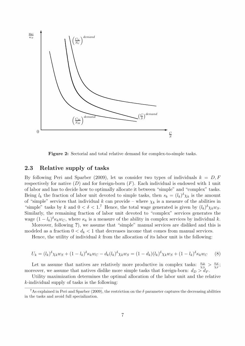
2.2 Relative demand for tasks
Workers are assumed to freely move between the two sectors, which implies that labor servicesare freely-mobile between the two sectors since they “travel” with workers.5
It is easy to obtain the sectorial relative demand for complex tasks as a function of relativetask wages, ω ≡ WC
WS:
CjSj
=
(1− βjβj
)σω−σ (6)
Since βM > βV for any given relative task wage, the service sector is always complex-taskintensive with respect to the manufacturing sector:6 CV
SV> CM
SM.
The total relative demand for complex tasks is then:
(C
S
)d= sM
(CMSM
)d+ (1− sM)
(CVSV
)d=
=
[s
s+ 1
(1− βMβM
)σ+
1
s+ 1
(1− βVβV
)σ]ω−σ (7)
where sM = SMSM+SV
=SMSV
SMSV
+1= s
s+1is the weight of the demand for simple tasks from the M
sector and increases when s = SMSV
increases.
4It is easy to obtain the straight relationship between the relative wage of tasks ω and the relative outputprice p ≡ pM
pV:
ω =
[(1− βM )p
σ−11−α − (1− βV )
βV − pσ−11−α βM
] 1σ−1
5We ought to notice that our estimated model is based on local labor market (using data at the provinciallevel); so, this latter hypothesis translates into a plausible “free workers mobility within the province”.
6We have absence of task-intensity reversal.
6
6
-
wC
wS
CS
(CM
SM
)demand
(CV
SV
)demand
0
(CS
)demand
1
Figure 2: Sectorial and total relative demand for complex-to-simple tasks.
2.3 Relative supply of tasks
By following Peri and Sparber (2009), let us consider two types of individuals k = D,Frespectively for native (D) and for foreign-born (F ). Each individual is endowed with 1 unitof labor and has to decide how to optimally allocate it between “simple” and “complex” tasks.Being lk the fraction of labor unit devoted to simple tasks, then sk = (lk)
δχk is the amountof “simple” services that individual k can provide – where χk is a measure of the abilities in“simple” tasks by k and 0 < δ < 1.7 Hence, the total wage generated is given by (lk)
δχkwS.Similarly, the remaining fraction of labor unit devoted to “complex” services generates thewage (1− lk)δκkwC , where κk is a measure of the ability in complex services by individual k.
Moreover, following ?), we assume that “simple” manual services are disliked and this ismodeled as a fraction 0 < dk < 1 that decreases income that comes from manual services.
Hence, the utility of individual k from the allocation of its labor unit is the following:
Uk = (lk)δχkwS + (1− lk)δκkwC − dk(lk)δχkwS = (1− dk)(lk)δχkwS + (1− lk)δκkwC (8)
Let us assume that natives are relatively more productive in complex tasks: κDχD
> κFχF
;moreover, we assume that natives dislike more simple tasks that foreign-born: dD > dF .
Utility maximization determines the optimal allocation of the labor unit and the relativek-individual supply of tasks is the following:
7As explained in Peri and Sparber (2009), the restriction on the δ parameter captures the decreasing abilitiesin the tasks and avoid full specialization.
7
cksk
=
(wCwS
) δ1−δ(
1
1− dk
) δ1−δ(κkχk
) 11−δ
(9)
for k = F,D. Not surprisingly, for the same relative wage a native individual D suppliesrelatively more complex tasks and this is due to to two different reasons: (a) natives arerelatively more productive in complex tasks, and (b) natives dislike more simple tasks.
We obtain the relative supply of tasks by weighing with the fraction of foreign-born supplyof manual services:
C
S≡ CF + CDSF + SD
≡ SFSF + SD
CFSF
+
(1− SF
SF + SD
)CDSD
= φ(f)cFsF
+ [1− φ(f)]cDsD
=
=
{φ(f)
(1
1− dF
) δ1−δ(κFχF
) 11−δ
+ [1− φ(f)]
(1
1− dD
) δ1−δ(κDχD
) 11−δ}(
wCwS
) δ1−δ
(10)
where f = LFLF+LD
is the fraction of foreign-born residents ; 0 < φ(·) < 1 is monotonicallyincreasing, φ(0) = 0 and φ(1) = 1.
When f increases there is a recomposition effect in favor of simple labor services and forany given relative wage there is a decrease in the relative supply of complex-to-simple tasks;
formally∂ CS
∂f< 0.
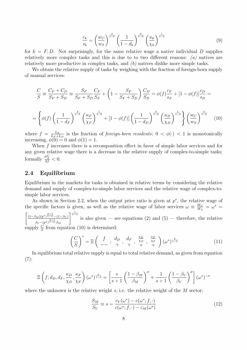
2.4 Equilibrium
Equilibrium in the markets for tasks is obtained in relative terms by considering the relativedemand and supply of complex-to-simple labor services and the relative wage of complex-to-simple labor services.
As shown in Section 2.2, when the output price ratio is given at p∗, the relative wage ofthe specific factors is given, as well as the relative wage of labor services ω ≡ WC
WS= ω∗ =
[(1−βM )(p∗)
σ−11−α−(1−βV )
βV −(p∗)σ−11−α βM
] 1σ−1
is also given — see equations (2) and (5) — therefore, the relative
supply CS
from equation (10) is determined:
(C
S
)∗= Ξ
(f−− ;
dD+
,dF+
,κDχD
+,
κFχF
+
)(ω∗)
δ1−δ (11)
In equilibrium total relative supply is equal to total relative demand, as given from equation(7):
Ξ
(f ; dD, dF ,
κDχD
,κFχF
)(ω∗)
δ1−δ =
[s
s+ 1
(1− βMβM
)σ+
1
s+ 1
(1− βVβV
)σ](ω∗)−σ
where the unknown is the relative weight s, i.e. the relative weight of the M sector:
SMSV≡ s =
cV (ω∗)− c(ω∗; f, ·)c(ω∗; f, ·)− cM(ω∗)
(12)
8
6
-
�
�
wC
wS
CS
(CS
)demand
1
(CS
)demand
0
(CS
)supply1
(CS
)supply0
E0
E ′
E ′′
0 (CS
)0
(CS
)′(CS
)′′
1
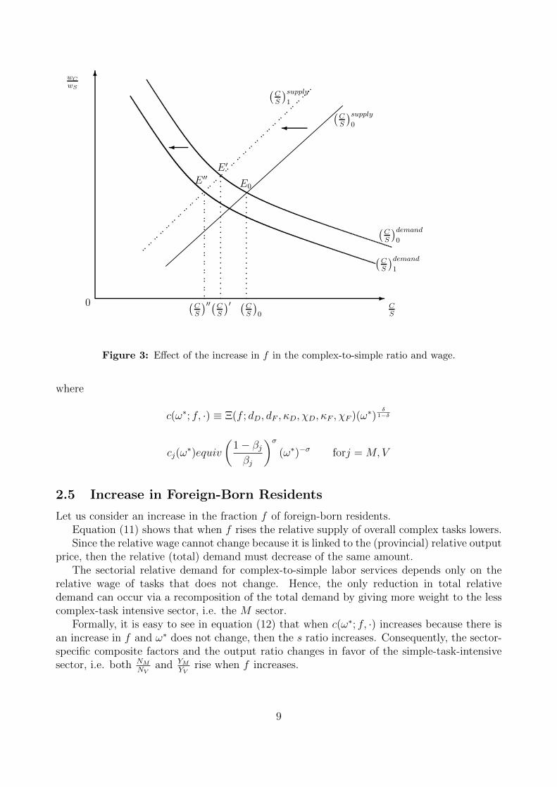
Figure 3: Effect of the increase in f in the complex-to-simple ratio and wage.
where
c(ω∗; f, ·) ≡ Ξ(f ; dD, dF , κD, χD, κF , χF )(ω∗)δ
1−δ
cj(ω∗)equiv
(1− βjβj
)σ(ω∗)−σ forj = M,V
2.5 Increase in Foreign-Born Residents
Let us consider an increase in the fraction f of foreign-born residents.Equation (11) shows that when f rises the relative supply of overall complex tasks lowers.Since the relative wage cannot change because it is linked to the (provincial) relative output
price, then the relative (total) demand must decrease of the same amount.The sectorial relative demand for complex-to-simple labor services depends only on the
relative wage of tasks that does not change. Hence, the only reduction in total relativedemand can occur via a recomposition of the total demand by giving more weight to the lesscomplex-task intensive sector, i.e. the M sector.
Formally, it is easy to see in equation (12) that when c(ω∗; f, ·) increases because there isan increase in f and ω∗ does not change, then the s ratio increases. Consequently, the sector-specific composite factors and the output ratio changes in favor of the simple-task-intensivesector, i.e. both NM
NVand YM
YVrise when f increases.
9
6 6
OM OVHM H ′M
VMPH ′MVMPHV
VMPHM
-
WH WH
W 0H
W ′H
1
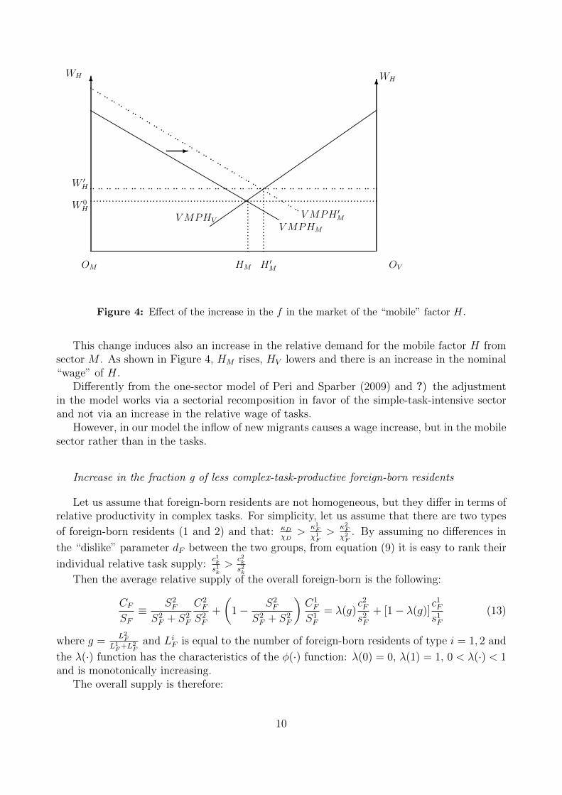
Figure 4: Effect of the increase in the f in the market of the “mobile” factor H.
This change induces also an increase in the relative demand for the mobile factor H fromsector M . As shown in Figure 4, HM rises, HV lowers and there is an increase in the nominal“wage” of H.
Differently from the one-sector model of Peri and Sparber (2009) and ?) the adjustmentin the model works via a sectorial recomposition in favor of the simple-task-intensive sectorand not via an increase in the relative wage of tasks.
However, in our model the inflow of new migrants causes a wage increase, but in the mobilesector rather than in the tasks.
Increase in the fraction g of less complex-task-productive foreign-born residents
Let us assume that foreign-born residents are not homogeneous, but they differ in terms ofrelative productivity in complex tasks. For simplicity, let us assume that there are two types
of foreign-born residents (1 and 2) and that: κDχD
>κ1Fχ1F>
κ2Fχ2F
. By assuming no differences in
the “dislike” parameter dF between the two groups, from equation (9) it is easy to rank their
individual relative task supply:c1ks1k>
c2ks2k
Then the average relative supply of the overall foreign-born is the following:
CFSF≡ S2
F
S2F + S2
F
C2F
S2F
+
(1− S2
F
S2F + S2
F
)C1F
S1F
= λ(g)c2Fs2F
+ [1− λ(g)]c1Fs1F
(13)
where g =L2F
L1F+L
2F
and LiF is equal to the number of foreign-born residents of type i = 1, 2 and
the λ(·) function has the characteristics of the φ(·) function: λ(0) = 0, λ(1) = 1, 0 < λ(·) < 1and is monotonically increasing.
The overall supply is therefore:
10
C
S≡ SFSF + SD
CFSF
+
(1− SF
SF + SD
)CDSD
= φ(f)cFsF
+ [1− φ(f)]cDsD
=
= φ(f)λ(g)c2Fs2F
+ φ(f)[1− λ(g)]c1Fs1F
+ [1− φ(f)]cDsD
(14)
An increase in g, i.e. in the fraction of less productive migrants in complex tasks, for agiven f , lowers the relative supply of complex tasks more since the composition effect givesmore weight to the migrants who are relatively less productive in complex tasks.
The same effects occurs in the market for the mobile factor H. Hence, the completerelationship between the relative output of manufacture-to-services is the following:
(YMYV
(f)
)=
(HM
HV
(f , g)+ +
)(1−α)(NM
NV
(f , g)+ +
)α(15)
3 Econometric Strategy
We estimate the causal impact of a relative inflows of migrants in province i at time t onthe relative added value of manufactures over services. We derive our estimated reduce formfrom the aforementioned theoretical model. Intuitively, a relative inflows of migrants in thelocal labor market generates an overall positive effects on the value added, but increases rela-tively more the production in the manufacture sector than service one. This reflects the factthat manufacturing production process involves relatively more simple tasks with respect toservices, and that migrants provide such tasks more likely than natives. This effect shouldappear more evident when the skills provided by a new inflow of migrant alters severely theworker skills distribution. In example, if a large number of arriving migrants are relatively lowskilled we should expect a stronger relative increase in manufacture value added. This doesnot mean necessarily that service value added is penalized by an increase in low skill migrants,in principle migrants arrival can help both productions.
A variation in the migrants to natives ratio is a reliable indicator for the changes in thelocal production process. As underlined in 15, a change in relative production is driven by achange in f , therefore in the relative abundance of simple to complex tasks. Even if this isunobserved in the data, a variation in the migrants to native ratio can approximate f giventhat migrants provide more likely simple tasks. This simplify a lot the specification of a re-duced form model. We use the logarithm of migrants to native ratio in province i at time t,lMNit, as our covariate of interest, specifying the econometric model:
yit = β0 + β1lMNit + X′
itβk + ηi + νt + εit (16)
Our dependent variable of interest yit is defined as the ration between the value addedin manufacture over service sectors in province i and time t, (V Aman/V Aserv)it. in orderto estimate β1 consistently, we need to address several econometric issues. First, as usuallyreported to the economic literature on migration we should expect that COV (lMNit, εit) 6= 0,this because of different reasons. Migrants location choices are not random, in fact, thereare two main drivers for this choice, which for simplicity we can call networks and economic
11
magnet effects, both these effects are variant over time so we need some kind of instrumentto exploit the variation from these effects to value added. Second, some provinces may shownatural or historical advantages that may affect value added raising time invariant unobservedheterogeneity (COMBES et al. 2010). Third, time specific factors can influence the provincialvalue added distribution, i.e. macroeconomic cycles, national political elections, national labormarket reforms etc. Fourth, E(εit | εit−1) will be considerably different from 0 in the valueadded series. (REFERNZA! – St. Bond Dynamic panel data model). Moreover when valueadded is very persistent over time computation of a static model may be difficult (Cassette& Edoardo 2012) both these considerations suggest a dynamic specification for our reduce formodel. In this new fashion equation 16 became:
(V Aman/V Aserv)it = β0 + ρ(V Aman/V Aserv)it−1 + β1lMNit + X′
itβk + ηi + νt + εit (17)
Where (V Aman/V Aserv)it−1 is an autoregressive term assuring that E(εit | εit−1) = 0, ηiis a provincial fixed effect controlling for unobserved time invariant heterogeneity and νt isa time specific fixed effect. Given model in 17 it seems reasonable to employ a Sys-GMMestimator a la Blundel and Bond in order to consistently estimate β1 (CITARE ). Moreover,such estimator provides several advantages, IVs is very well understood it allows discussion ofthe identifying assumptions and a number of useful tests for exogeneity while it is quite robustto functional forms assumptions. Endogeneity issues can be addressed through the use ofthe same method including a set of instruments Zit. In particular, considering the aforemen-tioned endogeneity problems Zit includes two year lag of the potentially endogenous covariates,namely the lagged dependent variable (V Aman/V Aserv)it−1 and the migrants to native ratiolMNit. The vector Xit contains a full set of controls for province i at time t, namely thelevel of migrants8, the degree of urbanization (as residents per squared kilometer), the aver-age skill level of the population (as the number of college graduates over the total population)and two measures on infrastructures quality (specifically the airports and highways extension).
Over the period 1995-2006 there were three major amnesties which considerably impacton migrant distribution, as typical for any such regularization, the actual presence of migrantsdates back before they appear in the official statistics. Hence, when including the incidence ofillegal migration, the profile of the time series would become smoother, but the trend wouldnot change. In order to control for that policy change we include in the vector Z a dummyvariable – which takes the value of one when the policy was implemented – interacted withthe consequent growth rate in residence permits registered in the province i9.
The robustness of our regression is evaluated with the classic tests after IV estimations, wereport Hansen-J test for all our estimations this ensures that the instrument are not correlatedwith the residuals, i.e. that the equation is not overidentified. To check for weak identifica-tion we include the Kleimbergen-Paap rank F-test for our instrumental variable estimations
8In defining GMM structure we consider as potentially endogenous such variable, but in this case we restrictthe set of instruments only to the equation in levels.
9The first major regularization law was passed in 1995 – around 250 thousands accepted applications.Then, in 1998 the “Turco-Napolitano” law resulted in the regularization of around 200 thousands migrants,and finally in 2002 the “Bossi-Fini” law induced amnesty included 640 thousands migrants over the next twoyears. See 5 in the next section
12
(KP2006). Given the dynamic specification we need to employ an Arellano Bond(1991) test,to prove that the residuals of the first differenced estimating equations are not second ordercorrelated. An accurate choice of the instrument solves the problem of instrument prolifera-tion (Roodman2009) the number of instrument used does not weaken the Hansen test statistic.
Given the fact that the number of elements in the matrix of instruments grows quadrati-cally in the time dimension, we want to be sure that the sample we are using contains adequateinformation to estimate them. In order to exclude the eventuality that our estimations areaffect by the so called ”small sample bias” we exploit the fact that estimating a dynamic modelwith OLS will produce an upward bias while estimate it using a FE estimator will generatea downward bias. We use the coefficients estimated via OLS and FE as upper and lowerbound for our preferred estimator (GMM-sys), as reported in 6, the autoregressive coefficientobtained through GMM actually lies the interval define by OLS and FE confirming that oursample contains enough information to ensure consistency of the estimator.
In order to control if the skill composition of migrants at province level plays a role in af-fecting the local production, we re-aggregate foreign workers in province i and time t into threeclasses according to the complexity of tasks they are more likely to provide. The rationale ofthat is related to the fact that the more the foreign workers are similar to natives, in termsof tasks they are likely to provide, the smaller should be the impact of a change in f to localproduction process. However we do not observe exactly the tasks provided by each worker,moreover educational data on migrants are rarely available for such a variety of countries andfor a long time span, a possible rough proxy can be represented by the level of developmentof the origin country, as approximated by the per-capita GDP. Since such approximation maybe difficult to hold country by country, here we use the ranking of origin countries on GDPper-capita distribution in order to distinguish three classes of rising educational attainmentamong the migrants10.
Finally, we test our theoretical model also with respect to export structure. A consol-idated branch of the empirical literature has highlighted the positive effect of migrants onbilateral trade, the rationale behind that, originally developed in Rauch (2001) and Rauchand Trinidade (2002), is that information costs plays a major role in the fixed cost that firmshave to pay to enter foreign markets and ethnic networks are likely to reduce some of theseinformation costs. Cross-border networks of people sharing the same country of origin cansubstitute or integrate organized markets in matching international demand and supply. More-over, immigrant networks may provide contract enforcement through sanctions and exclusions,which substitutes for weak institutional rules and reduces trade costs (Briant et al., 2009).While the aforementioned channels have been deeply scrutinized, less attention has been pro-vided on sectoral export composition. Starting from the empirical evidence on value added,which underline a positive effect of migrants on low skill intense production, we want to testour results also with respect to exports. Intuitively, if a change of workers skill compositiondo have an effect on production process we should expect a similar outcome also on exportcomposition, if we assume that production is not totally absorbed by the local market. Thatwhy in the next set of regressions we define a new dependent variable as the ratio betweenlow/high technology exports at province level.
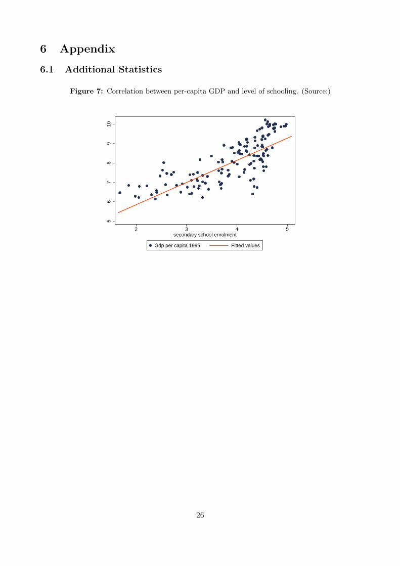
10As reported in 7 in 6 countries’ per capita GDP is indeed highly correlated with schooling attainment.
13
3.1 Data and Descriptive Statistics
The main objective of this paper is to analyze the impact of migration11 on the production andthe export structure of the Italian economy over the period of more intense and significant in-crease in foreign-born presence, 1995-2006. In the following sections we report some importantcharacteristics of the migration phenomenon in Italy and of the production structure.
The analysis is conducted at the level of Province, i.e. NUTS3. We recall that the 103Italian provinces12 have an average size of 2,800 square km with a coefficient of variationat 0.17. They are 57 times tinier than American states and more than 200 times smallerthan the Canadian provinces. They are also smaller and more regular in size with respect toFrench metropolitan departements and Spanish provinces. We deem the Province as the finestgeographical entity to investigate migration externalities and the choice of this geographicallevel is justified by two main reasons. First, detailed data on residence permits, includingorigin countries, are not available at a finer level than the Province. Second, the fact of beingwell-confined areas allows us to avoid the size effect of the Modifiable Area Unit Problem –MAUP (see Briant et al. (2010) on the issue). This same geographical entity is used in Brattiet al (2012) for an analysis of the pro-trade effect of migration and in Jayet et al (2010) tostudy the network effect on Italian migration.
3.1.1 Migration Origin and Location in Italy
Migration in Italy has been characterized by two main stylized facts. First, it has been a veryrapid phenomenon. Second, due to absence of strong colonial links, migration into Italy hasbeen more diversified in terms of origin countries than in any other European country (189 isthe number of nationalities currently present). Migration to Italy has increased by a factor of3 in slightly more than a decade. The presence of the foreign-born individuals increased from1.4 million in 2002 to 4.6 million in 2011, which equals 7.6% of the Italian population.
Figure 5 reports a measure of the rising stock of foreign-born presence in 1995-2006, asmeasured by the number of residence permits which are the data we use in this paper.13 De-tailed measures of residence permits can go back to 1992, but we use 1995 as the starting yearsince previous years were not reliable and less representative of the migration phenomenondue to low numbers, especially when considering data at the provincial level. Due to the EUEastern enlargement in 2004-2007, the requirement for residence and work permits has beenlevied for some relevant nationalities (like Romanians and Polish). So, we considered 2006 asthe ending year of our study.
When investigating more thoroughly this rapid increase in foreign presence, two charac-teristics ought to be noticed: first, the rapid change also in the composition of migration bycountry of origin; second, the uneven localization of migrants in the Italian territory. As amatter of fact, the rapid increase in the foreign-born population was also characterized by a
11We refer here to migration as measured by stock of foreign-born individuals. No data on pure flows areavailable in Italy at the disaggregated level we investigate; hence, when we address “flows” we are actuallyusing stock variations.
12The number of Province changes over the sample period due to the creation of new provinces. We usedata that consider the 1995 distribution of 103 entities.
13They slightly differ from the data on population registers since minors are not counted since they areincluded in the residence permits of their custodians. Data on residence permits are released by ISTAT, butthey refer to data from the Ministry of the Interior through their local offices (Questure).
14
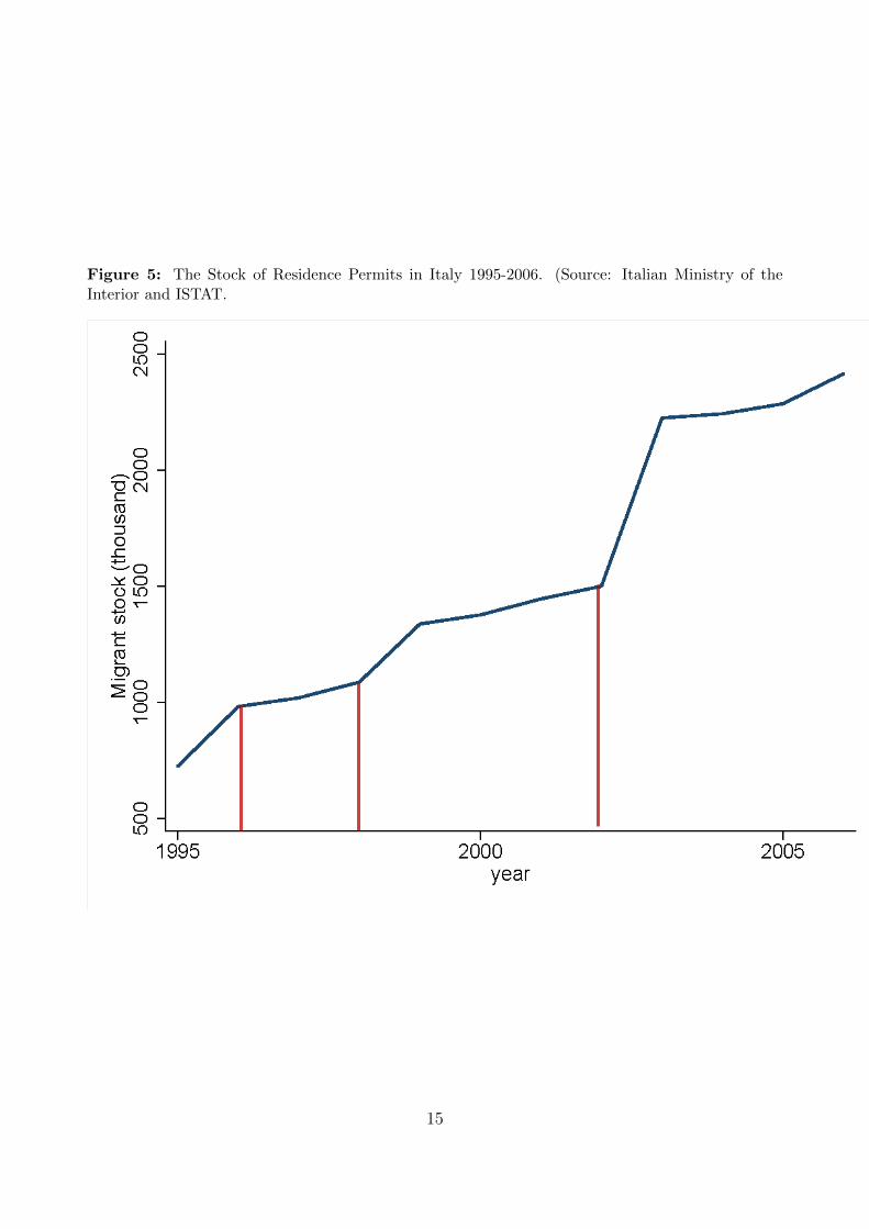
Figure 5: The Stock of Residence Permits in Italy 1995-2006. (Source: Italian Ministry of theInterior and ISTAT.
15
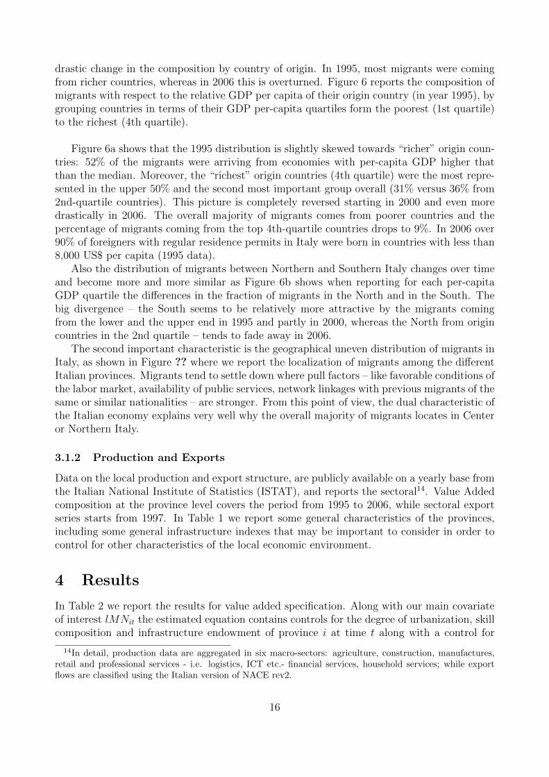
drastic change in the composition by country of origin. In 1995, most migrants were comingfrom richer countries, whereas in 2006 this is overturned. Figure 6 reports the composition ofmigrants with respect to the relative GDP per capita of their origin country (in year 1995), bygrouping countries in terms of their GDP per-capita quartiles form the poorest (1st quartile)to the richest (4th quartile).
Figure 6a shows that the 1995 distribution is slightly skewed towards “richer” origin coun-tries: 52% of the migrants were arriving from economies with per-capita GDP higher thatthan the median. Moreover, the “richest” origin countries (4th quartile) were the most repre-sented in the upper 50% and the second most important group overall (31% versus 36% from2nd-quartile countries). This picture is completely reversed starting in 2000 and even moredrastically in 2006. The overall majority of migrants comes from poorer countries and thepercentage of migrants coming from the top 4th-quartile countries drops to 9%. In 2006 over90% of foreigners with regular residence permits in Italy were born in countries with less than8,000 US$ per capita (1995 data).
Also the distribution of migrants between Northern and Southern Italy changes over timeand become more and more similar as Figure 6b shows when reporting for each per-capitaGDP quartile the differences in the fraction of migrants in the North and in the South. Thebig divergence – the South seems to be relatively more attractive by the migrants comingfrom the lower and the upper end in 1995 and partly in 2000, whereas the North from origincountries in the 2nd quartile – tends to fade away in 2006.
The second important characteristic is the geographical uneven distribution of migrants inItaly, as shown in Figure ?? where we report the localization of migrants among the differentItalian provinces. Migrants tend to settle down where pull factors – like favorable conditions ofthe labor market, availability of public services, network linkages with previous migrants of thesame or similar nationalities – are stronger. From this point of view, the dual characteristic ofthe Italian economy explains very well why the overall majority of migrants locates in Centeror Northern Italy.
3.1.2 Production and Exports
Data on the local production and export structure, are publicly available on a yearly base fromthe Italian National Institute of Statistics (ISTAT), and reports the sectoral14. Value Addedcomposition at the province level covers the period from 1995 to 2006, while sectoral exportseries starts from 1997. In Table 1 we report some general characteristics of the provinces,including some general infrastructure indexes that may be important to consider in order tocontrol for other characteristics of the local economic environment.
4 Results
In Table 2 we report the results for value added specification. Along with our main covariateof interest lMNit the estimated equation contains controls for the degree of urbanization, skillcomposition and infrastructure endowment of province i at time t along with a control for
14In detail, production data are aggregated in six macro-sectors: agriculture, construction, manufactures,retail and professional services - i.e. logistics, ICT etc.- financial services, household services; while exportflows are classified using the Italian version of NACE rev2.
16
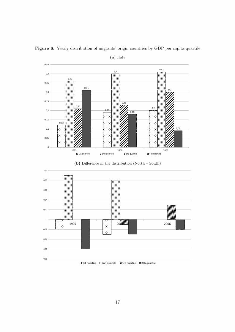
Figure 6: Yearly distribution of migrants’ origin countries by GDP per capita quartile
(a) Italy
0,12
0,190,2
0,36
0,40,41
0,21
0,23
0,30,31
0,18
0,09
0
0,05
0,1
0,15
0,2
0,25
0,3
0,35
0,4
0,45
1995 2000 2006
1st quartile 2nd quartile 3rd quartile 4th quartile
(b) Difference in the distribution (North – South)
-0,08
-0,06
-0,04
-0,02
0
0,02
0,04
0,06
0,08
0,1
1995 2000 2006
1st quartile 2nd quartile 3rd quartile 4th quartile
17
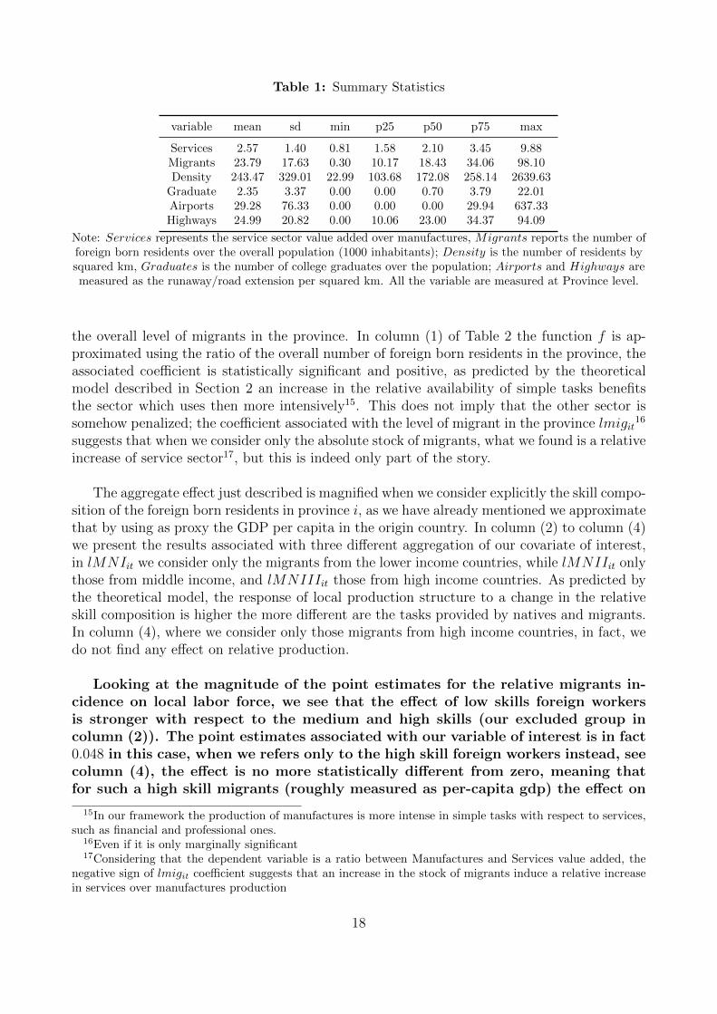
Table 1: Summary Statistics
variable mean sd min p25 p50 p75 max
Services 2.57 1.40 0.81 1.58 2.10 3.45 9.88Migrants 23.79 17.63 0.30 10.17 18.43 34.06 98.10Density 243.47 329.01 22.99 103.68 172.08 258.14 2639.63
Graduate 2.35 3.37 0.00 0.00 0.70 3.79 22.01Airports 29.28 76.33 0.00 0.00 0.00 29.94 637.33Highways 24.99 20.82 0.00 10.06 23.00 34.37 94.09
Note: Services represents the service sector value added over manufactures, Migrants reports the number offoreign born residents over the overall population (1000 inhabitants); Density is the number of residents bysquared km, Graduates is the number of college graduates over the population; Airports and Highways aremeasured as the runaway/road extension per squared km. All the variable are measured at Province level.
the overall level of migrants in the province. In column (1) of Table 2 the function f is ap-proximated using the ratio of the overall number of foreign born residents in the province, theassociated coefficient is statistically significant and positive, as predicted by the theoreticalmodel described in Section 2 an increase in the relative availability of simple tasks benefitsthe sector which uses then more intensively15. This does not imply that the other sector issomehow penalized; the coefficient associated with the level of migrant in the province lmigit
16
suggests that when we consider only the absolute stock of migrants, what we found is a relativeincrease of service sector17, but this is indeed only part of the story.
The aggregate effect just described is magnified when we consider explicitly the skill compo-sition of the foreign born residents in province i, as we have already mentioned we approximatethat by using as proxy the GDP per capita in the origin country. In column (2) to column (4)we present the results associated with three different aggregation of our covariate of interest,in lMNIit we consider only the migrants from the lower income countries, while lMNIIit onlythose from middle income, and lMNIIIit those from high income countries. As predicted bythe theoretical model, the response of local production structure to a change in the relativeskill composition is higher the more different are the tasks provided by natives and migrants.In column (4), where we consider only those migrants from high income countries, in fact, wedo not find any effect on relative production.
Looking at the magnitude of the point estimates for the relative migrants in-cidence on local labor force, we see that the effect of low skills foreign workersis stronger with respect to the medium and high skills (our excluded group incolumn (2)). The point estimates associated with our variable of interest is in fact0.048 in this case, when we refers only to the high skill foreign workers instead, seecolumn (4), the effect is no more statistically different from zero, meaning thatfor such a high skill migrants (roughly measured as per-capita gdp) the effect on
15In our framework the production of manufactures is more intense in simple tasks with respect to services,such as financial and professional ones.
16Even if it is only marginally significant17Considering that the dependent variable is a ratio between Manufactures and Services value added, the
negative sign of lmigit coefficient suggests that an increase in the stock of migrants induce a relative increasein services over manufactures production
18
production is not different from the excluded group (medium-low skills). Givingour identification strategy, which consider each group in a separated regression,mainly in order to be more parsimonious and avoiding that number of instrumentsraises18, we do not comment directly the coefficient associated with the mediumskill regression (column 3) because in such case the reference group contains bothlow and high skills migrant workers and possibly confounding the relative effectof medium skilled.
Furthermore, we employ a different classification of foreign born workers ac-cording to their schooling attainment, in order to proxy their skill level moreprecisely. In particular we use the information compiled by (Docquier et al.,2008) which classify foreign born residence in OECD countries by nationality andschooling attainment19. For each province i we consider the share of low skillforeign workers aggregating the stock of migrants according to the source countryshare of primary school attainment20. Table 3 reports the estimates of skills spe-cific regression using the (Docquier et al., 2008) classification. As we can see fromcolumn(1) the coefficient associated with the low skill foreign workers is higherwith respect to the excluded group (medium-high skills), while the one associatedto the high-skill migrants is lower and only marginally different from zero.
The same results hold when we consider as dependent variable the ration be-tween low to high technology exports21, see Table 2, also in this case the magnitudeof the effect is much stronger when we consider only those workers which are morelikely to provide simpler tasks with respect to natives, column (2). Same resultsholds when we classify foreign born workers according to the level of schooling,in table 5, column (1) reports the point estimates for the low skill with respect tomedium and high skill foreign worker, again the impact is much stronger for suchgroup, while the same effect considering only the high skill fraction of migrants isnot statistically . Across specifications one main result emerge robust and stable,the relative concentration of immigrants at province level, causes a shift in thelocal production bundle towards manufacturing with respect to services. Thisresult, confirmed throughout the different model specifications (see Table 2 4),seems to confirm the theoretical explanation we gave in the previous section.However another very interesting result, that emerge when we use schooling asmeasure of foreign workers skills, which indeed is a more accurate proxy for themigrant skill composition, is the significative coefficient associated with the rela-tive availability of high skills migrants, see column(3) 5; this effect, in fact, seemsto be associated to the fact that even if some high skilled workers are likely to
18Such a concern is motivated by the structure of our panel, which reports only 103 different individuals –Italian Provinces, given the fact that the number of elements in the estimated variance matrix is quadratic inthe instrument count (as in T ), a relatively finite sample, as ours, may lack adequate information to estimatelarge matrix.
19Specifically, the stock (and rates) of migration inflows for each OECD country are provided by level ofschooling and gender for 195 source countries in 1990 and 2000
20In such a way we do not exclude any nationality in building our skill specific lMN but we consider onlythe fraction of residence which reports a specific school attainment. Of course in doing so we implicitly assumethat, by nationality, the distribution of skills over Italy is uniform.
21As relatively higher technology export industries we consider chemicals and rubber, pharmaceutical prod-ucts, computers and electronic devices
19

provide the same kind of tasks with respect to natives they are somehow under-employed. There may be then a discrimination in the labor market which resultin a significant skill waste.
20
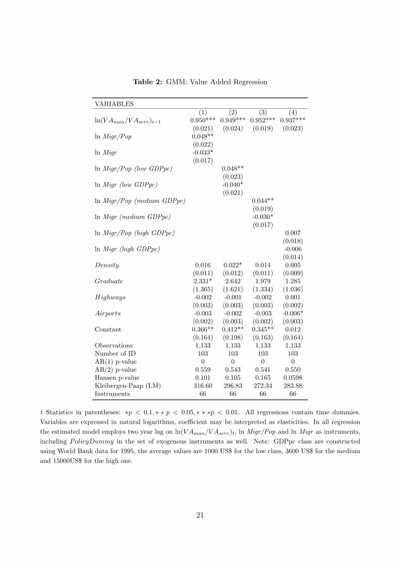
Table 2: GMM: Value Added Regression
VARIABLES(1) (2) (3) (4)
ln(V Aman/V Aserv)t−1 0.950*** 0.949*** 0.952*** 0.937***(0.021) (0.024) (0.019) (0.023)
ln Migr/Pop 0.048**(0.022)
ln Migr -0.033*(0.017)
ln Migr/Pop (low GDPpc) 0.048**(0.023)
ln Migr (low GDPpc) -0.040*(0.021)
ln Migr/Pop (medium GDPpc) 0.044**(0.019)
ln Migr (medium GDPpc) -0.030*(0.017)
ln Migr/Pop (high GDPpc) 0.007(0.018)
ln Migr (high GDPpc) -0.006(0.014)
Density 0.016 0.022* 0.014 0.005(0.011) (0.012) (0.011) (0.009)
Graduate 2.331* 2.642 1.979 1.285(1.365) (1.621) (1.334) (1.036)
Highways -0.002 -0.001 -0.002 0.001(0.003) (0.003) (0.003) (0.002)
Airports -0.003 -0.002 -0.003 -0.006*(0.002) (0.003) (0.002) (0.003)
Constant 0.366** 0.412** 0.345** 0.012(0.164) (0.198) (0.163) (0.164)
Observations 1,133 1,133 1,133 1,133Number of ID 103 103 103 103AR(1) p-value 0 0 0 0AR(2) p-value 0.559 0.543 0.541 0.550Hansen p-value 0.101 0.105 0.165 0.0598Kleibergen-Paap (LM) 316.60 296.83 272.34 283.88Instruments 66 66 66 66
t Statistics in parentheses: ∗p < 0.1, ∗ ∗ p < 0.05, ∗ ∗ ∗p < 0.01. All regressions contain time dummies.
Variables are expressed in natural logarithms, coefficient may be interpreted as elasticities. In all regression
the estimated model employs two year lag on ln(V Aman/V Aserv)t, ln Migr/Pop and ln Migr as instruments,
including PolicyDummy in the set of exogenous instruments as well. Note: GDPpc class are constructed
using World Bank data for 1995, the average values are 1000 US$ for the low class, 3600 US$ for the medium
and 15000US$ for the high one.
21
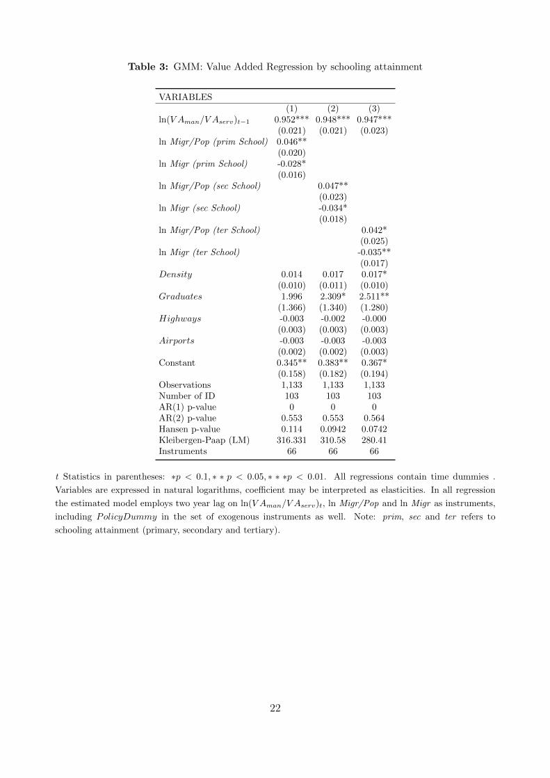
Table 3: GMM: Value Added Regression by schooling attainment
VARIABLES(1) (2) (3)
ln(V Aman/V Aserv)t−1 0.952*** 0.948*** 0.947***(0.021) (0.021) (0.023)
ln Migr/Pop (prim School) 0.046**(0.020)
ln Migr (prim School) -0.028*(0.016)
ln Migr/Pop (sec School) 0.047**(0.023)
ln Migr (sec School) -0.034*(0.018)
ln Migr/Pop (ter School) 0.042*(0.025)
ln Migr (ter School) -0.035**(0.017)
Density 0.014 0.017 0.017*(0.010) (0.011) (0.010)
Graduates 1.996 2.309* 2.511**(1.366) (1.340) (1.280)
Highways -0.003 -0.002 -0.000(0.003) (0.003) (0.003)
Airports -0.003 -0.003 -0.003(0.002) (0.002) (0.003)
Constant 0.345** 0.383** 0.367*(0.158) (0.182) (0.194)
Observations 1,133 1,133 1,133Number of ID 103 103 103AR(1) p-value 0 0 0AR(2) p-value 0.553 0.553 0.564Hansen p-value 0.114 0.0942 0.0742Kleibergen-Paap (LM) 316.331 310.58 280.41Instruments 66 66 66
t Statistics in parentheses: ∗p < 0.1, ∗ ∗ p < 0.05, ∗ ∗ ∗p < 0.01. All regressions contain time dummies .
Variables are expressed in natural logarithms, coefficient may be interpreted as elasticities. In all regression
the estimated model employs two year lag on ln(V Aman/V Aserv)t, ln Migr/Pop and ln Migr as instruments,
including PolicyDummy in the set of exogenous instruments as well. Note: prim, sec and ter refers to
schooling attainment (primary, secondary and tertiary).
22
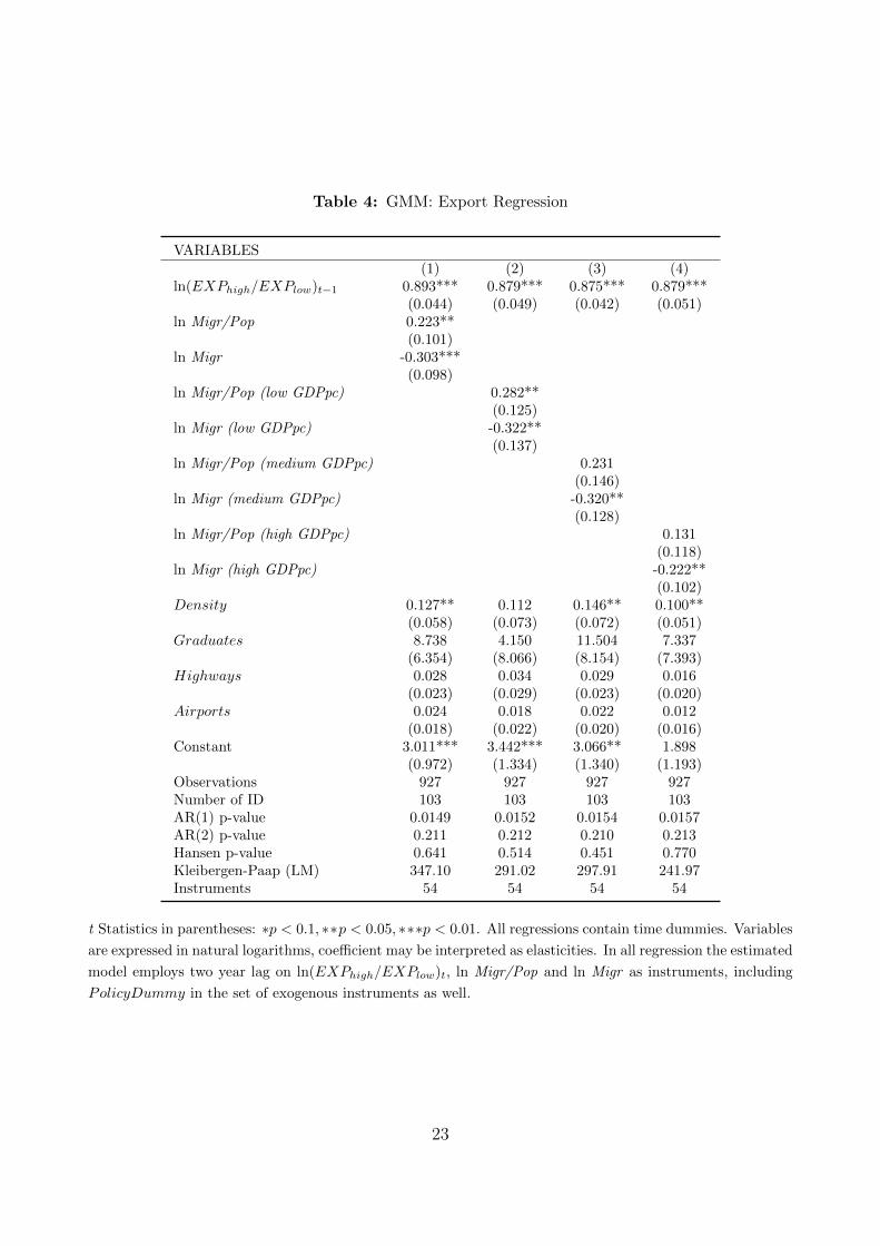
Table 4: GMM: Export Regression
VARIABLES(1) (2) (3) (4)
ln(EXPhigh/EXPlow)t−1 0.893*** 0.879*** 0.875*** 0.879***(0.044) (0.049) (0.042) (0.051)
ln Migr/Pop 0.223**(0.101)
ln Migr -0.303***(0.098)
ln Migr/Pop (low GDPpc) 0.282**(0.125)
ln Migr (low GDPpc) -0.322**(0.137)
ln Migr/Pop (medium GDPpc) 0.231(0.146)
ln Migr (medium GDPpc) -0.320**(0.128)
ln Migr/Pop (high GDPpc) 0.131(0.118)
ln Migr (high GDPpc) -0.222**(0.102)
Density 0.127** 0.112 0.146** 0.100**(0.058) (0.073) (0.072) (0.051)
Graduates 8.738 4.150 11.504 7.337(6.354) (8.066) (8.154) (7.393)
Highways 0.028 0.034 0.029 0.016(0.023) (0.029) (0.023) (0.020)
Airports 0.024 0.018 0.022 0.012(0.018) (0.022) (0.020) (0.016)
Constant 3.011*** 3.442*** 3.066** 1.898(0.972) (1.334) (1.340) (1.193)
Observations 927 927 927 927Number of ID 103 103 103 103AR(1) p-value 0.0149 0.0152 0.0154 0.0157AR(2) p-value 0.211 0.212 0.210 0.213Hansen p-value 0.641 0.514 0.451 0.770Kleibergen-Paap (LM) 347.10 291.02 297.91 241.97Instruments 54 54 54 54
t Statistics in parentheses: ∗p < 0.1, ∗∗p < 0.05, ∗∗∗p < 0.01. All regressions contain time dummies. Variables
are expressed in natural logarithms, coefficient may be interpreted as elasticities. In all regression the estimated
model employs two year lag on ln(EXPhigh/EXPlow)t, ln Migr/Pop and ln Migr as instruments, including
PolicyDummy in the set of exogenous instruments as well.
23
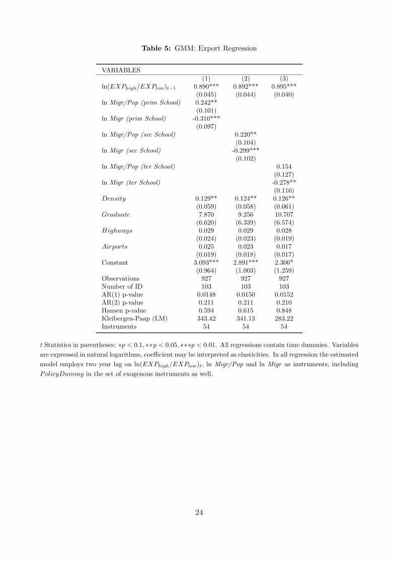
Table 5: GMM: Export Regression
VARIABLES(1) (2) (3)
ln(EXPhigh/EXPlow)t−1 0.890*** 0.892*** 0.895***(0.045) (0.044) (0.040)
ln Migr/Pop (prim School) 0.242**(0.101)
ln Migr (prim School) -0.310***(0.097)
ln Migr/Pop (sec School) 0.220**(0.104)
ln Migr (sec School) -0.299***(0.102)
ln Migr/Pop (ter School) 0.154(0.127)
ln Migr (ter School) -0.278**(0.116)
Density 0.129** 0.124** 0.126**(0.059) (0.058) (0.061)
Graduate 7.870 9.256 10.707(6.620) (6.339) (6.574)
Highways 0.029 0.029 0.028(0.024) (0.023) (0.019)
Airports 0.025 0.023 0.017(0.019) (0.018) (0.017)
Constant 3.093*** 2.891*** 2.306*(0.964) (1.003) (1.259)
Observations 927 927 927Number of ID 103 103 103AR(1) p-value 0.0148 0.0150 0.0152AR(2) p-value 0.211 0.211 0.210Hansen p-value 0.594 0.615 0.848Kleibergen-Paap (LM) 343.42 341.13 283.22Instruments 54 54 54
t Statistics in parentheses: ∗p < 0.1, ∗∗p < 0.05, ∗∗∗p < 0.01. All regressions contain time dummies. Variables
are expressed in natural logarithms, coefficient may be interpreted as elasticities. In all regression the estimated
model employs two year lag on ln(EXPhigh/EXPlow)t, ln Migr/Pop and ln Migr as instruments, including
PolicyDummy in the set of exogenous instruments as well.
24
5 Concluding remarks
References
Altonji, J. and Card, D. (1991). The effects of immigration on the labor market outcomesof less-skilled natives. In Abowd, J. and Freeman, R., editors, Immigration, Trade and theLabor Market. University of Chicago Press.
Briant, A., Combes, P.-P., and Lafourcade, M. (2010). Dots to boxes: Do the size and shapeof spatial units jeopardize economic geography estimations? Journal of Urban Economics,67:287–302.
Docquier, F., Lowell, B. L., and Marfouk, A. (2008). A gendered assessment of the braindrain. Policy Research Working Paper Series 4613, The World Bank.
Peri, G. and Sparber, C. (2009). Task specialization, immigration, and wages. AmericanEconomic Journal: Applied Economics, 1(3):135–69.
25
6 Appendix
6.1 Additional Statistics
Figure 7: Correlation between per-capita GDP and level of schooling. (Source:)
56
78
910
2 3 4 5secondary school enrolment
Gdp per capita 1995 Fitted values
26
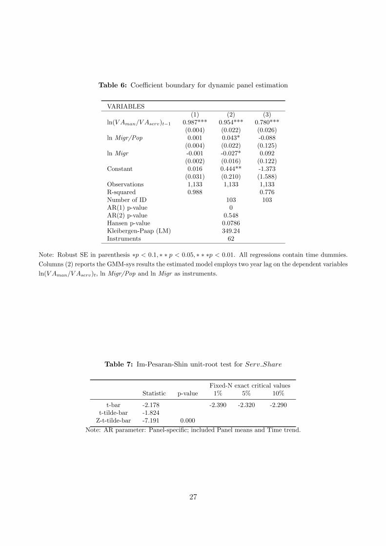
Table 6: Coefficient boundary for dynamic panel estimation
VARIABLES(1) (2) (3)
ln(V Aman/V Aserv)t−1 0.987*** 0.954*** 0.780***(0.004) (0.022) (0.026)
ln Migr/Pop 0.001 0.043* -0.088(0.004) (0.022) (0.125)
ln Migr -0.001 -0.027* 0.092(0.002) (0.016) (0.122)
Constant 0.016 0.444** -1.373(0.031) (0.210) (1.588)
Observations 1,133 1,133 1,133R-squared 0.988 0.776Number of ID 103 103AR(1) p-value 0AR(2) p-value 0.548Hansen p-value 0.0786Kleibergen-Paap (LM) 349.24Instruments 62
Note: Robust SE in parenthesis ∗p < 0.1, ∗ ∗ p < 0.05, ∗ ∗ ∗p < 0.01. All regressions contain time dummies.
Columns (2) reports the GMM-sys results the estimated model employs two year lag on the dependent variables
ln(V Aman/V Aserv)t, ln Migr/Pop and ln Migr as instruments.
Table 7: Im-Pesaran-Shin unit-root test for Serv Share
Fixed-N exact critical valuesStatistic p-value 1% 5% 10%
t-bar -2.178 -2.390 -2.320 -2.290t-tilde-bar -1.824
Z-t-tilde-bar -7.191 0.000
Note: AR parameter: Panel-specific; included Panel means and Time trend.
27
6.2 Robustness Check: Baseline model
In this section we reports some robustness check of the baseline econometric model, usingtwo different instrumental variable for the actual stock of migrants. The first one is maybethe most accepted instrument based on the original idea of (Altonji and Card, 1991) onimmigrants enclaves. The basic idea is that immigrants tend to settle where there are alreadyestablished communities from the same country: this, in fact, may reducing migration costsand maximize benefits (probability to find an accommodation or a job for example), underthe assumption that this dynamic provides an exogenous source of variation for immigrationstocks. In our case we use the first year of available data on residence permits in Italy,1991, and, based on the distribution of nationality across provinces in that year, we constructpredicted stock of immigrants for the period 1995-2006, using the predicted stock to computeour covariates of interests lMN and lmig. Since in 1991 the number of Italian provinces was95, in constructing our instrument we follows two approaches, in column (1) 8 we consider onlythe provinces already operating in the 1991, while in column (2) we rescale the distribution in1991 according to the regional population shares ini 1995 – the first year with 103 operatingprovinces.The second approach we follow in order to build an instrument for the actual stock of migrantsis to regress the immigration growth rate on a set of dummies and predict an expected growthrate, which we then use to impute the actual stock22. In detail, the predicted growth rate isbased on the following regression:
mig growtijt = αit + αjt + αij + εijt (18)
22In this case we consider only those nationalities that were already present in Italy in 1995
28
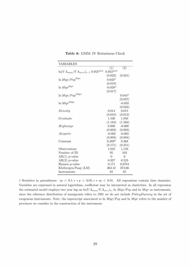
Table 8: GMM: IV Robustness Check
VARIABLES(1) (2)
ln(V Aman/V Aserv)t−1 0.953*** 0.953***(0.022) (0.021)
lnMigr/Pop95pr
0.033*(0.019)
lnMigr95pr -0.028*(0.017)
lnMigr/Pop103pr
0.044*(0.027)
lnMigr103pr -0.033(0.023)
Density 0.014 0.015(0.010) (0.012)
Graduate 1.530 1.850(1.184) (1.563)
Highways 0.000 -0.000(0.003) (0.003)
Airports -0.002 -0.003(0.003) (0.004)
Constant 0.289* 0.368(0.171) (0.251)
Observations 1,045 1,133Number of ID 95 103AR(1) p-value 0 0AR(2) p-value 0.327 0.523Hansen p-value 0.171 0.0784Kleibergen-Paap (LM) 363.31 373.66Instruments 65 65
t Statistics in parentheses: ∗p < 0.1, ∗ ∗ p < 0.05, ∗ ∗ ∗p < 0.01. All regressions contain time dummies.
Variables are expressed in natural logarithms, coefficient may be interpreted as elasticities. In all regression
the estimated model employs two year lag on ln(V Aman/V Aserv)t, ln Migr/Pop and ln Migr as instruments,
since the reference distribution of immigrants refers to 1991 we do not include PolicyDummy in the set of
exogenous instruments. Note: the superscript associated to ln Migr/Pop and ln Migr refers to the number of
provinces we consider in the construction of the instrument.
29