Embed Size (px)
Citation preview

MIMO Controller Design for aSCARA Robot
F.P.M. Dullens
DCT 2008.024
Traineeship report
Coach(es): Ph.D. He Yun BoPh.D. Zhang Chi
Supervisor: Prof. OuProf. Dr. H. Nijmeijer
Technische Universiteit EindhovenDepartment Mechanical EngineeringDynamics and Control Group
Eindhoven, February, 2008

2

Contents
1 Introduction 51.1 Objective and Problem Statement . . . . . . . . . . . . . . . . . . . 51.2 Overview . . . . . . . . . . . . . . . . . . . . . . . . . . . . . . . . 5
2 Robot Modeling 72.1 Experimental Setup . . . . . . . . . . . . . . . . . . . . . . . . . . 72.2 Robot Dynamics . . . . . . . . . . . . . . . . . . . . . . . . . . . . 92.3 Estimation of Model Parameters . . . . . . . . . . . . . . . . . . . 102.4 Model Verification . . . . . . . . . . . . . . . . . . . . . . . . . . . 122.5 Inverse Kinematics . . . . . . . . . . . . . . . . . . . . . . . . . . . 16
3 Decoupling Control 193.1 Decoupling via Computed Torque Control . . . . . . . . . . . . . . 193.2 Input-Output Linearization andDecoupling via Restricted State Feed-
back with Disturbance Rejection . . . . . . . . . . . . . . . . . . . 223.3 Decoupling Control including Motor Dynamics with Disturbance
Decoupling . . . . . . . . . . . . . . . . . . . . . . . . . . . . . . . 223.4 Decoupling Controller based on LS-SVM . . . . . . . . . . . . . . 233.5 Conclusion . . . . . . . . . . . . . . . . . . . . . . . . . . . . . . . 23
4 Feedback Control Design for the Decoupled System 254.1 Dynamics after Decoupling . . . . . . . . . . . . . . . . . . . . . . 254.2 Outer Loop Controller . . . . . . . . . . . . . . . . . . . . . . . . . 264.3 Simulation Results . . . . . . . . . . . . . . . . . . . . . . . . . . . 304.4 Conclusion . . . . . . . . . . . . . . . . . . . . . . . . . . . . . . . 31
5 Implementation 335.1 Implementation on a SCARA Platform . . . . . . . . . . . . . . . . 335.2 Discrete Time Conversions . . . . . . . . . . . . . . . . . . . . . . 34
6 Experimental Results 376.1 Dynamics after Decoupling . . . . . . . . . . . . . . . . . . . . . . 376.2 Control Design . . . . . . . . . . . . . . . . . . . . . . . . . . . . . 396.3 Experimental Results . . . . . . . . . . . . . . . . . . . . . . . . . . 406.4 Conclusion . . . . . . . . . . . . . . . . . . . . . . . . . . . . . . . 44
7 Adaptive Control Design for Vertical Stage 457.1 modeling . . . . . . . . . . . . . . . . . . . . . . . . . . . . . . . . 457.2 Adaptive Control . . . . . . . . . . . . . . . . . . . . . . . . . . . . 467.3 Simulation Results . . . . . . . . . . . . . . . . . . . . . . . . . . . 487.4 Experimental Results . . . . . . . . . . . . . . . . . . . . . . . . . 497.5 Conclusion . . . . . . . . . . . . . . . . . . . . . . . . . . . . . . . 51
3

8 Conclusions and Recommendations 538.1 Conclusions . . . . . . . . . . . . . . . . . . . . . . . . . . . . . . 538.2 Recommendations . . . . . . . . . . . . . . . . . . . . . . . . . . . 54
A Robot Dynamics 57
B Coupling of Robot Dynamics 58
C Dynamic Equation as Function of Base Parameter Set 63
D Relation Digital Input to Torque 64
E Model Verification 65
F Input-Output Linearization and Decoupling via Restricted State Feedbackwith Disturbance Rejection 67F.1 Theory . . . . . . . . . . . . . . . . . . . . . . . . . . . . . . . . . 67F.2 Applied to SCARA . . . . . . . . . . . . . . . . . . . . . . . . . . . 69
G Prediction Decoupling Effect 73G.1 Decoupling for Parameter Error . . . . . . . . . . . . . . . . . . . . 73G.2 Decoupling for Payload . . . . . . . . . . . . . . . . . . . . . . . . 74
H Velocity Fit 4 Khz 76
I Gains SISO Controllers for Decoupled System 78
J Decentralized Control 79
K Experimental Results 83
L Conversion from Velocity to Position 90
M Delay 91
N PD Control of Vertical Axis 92
4

1 Introduction
The main electric component stored in today’s luxury apparatus like for exampletelephones and DVD-players are chips. Before a chip is ready to be used, it hasto undergo many production processes. This production process is divided intoso-called front-end and back-end. Front end processing refers to a multiple-stepsequence of photographic and chemical processing steps during which electroniccircuits are gradually created on a wafer made of pure semiconducting material.Once tested, the wafer is scored and then broken into individual dice. Back-endprocessing involves mounting the die, connecting the die pads to the pins on thepackage, and sealing the die.
Wafers are thus of key importance in the fabrication of semiconductor devices.In order to move the wafer from one production process to another, a robotic armcan be used. In this work a direct drive SCARA (Selective Compliant ArticulatedRobot for Assembly) robot is considered to perform this job (see figure 1.1).
1.1 Objective and Problem Statement
Since the motors of the SCARA are directly attached to the link, i.e. without useof gears, an input to one of the joints will also disturb the other joints due to thecoupling of the system. This is called a direct drive actuator system. Anotherdifficulty for control arises due to changing inertia for each joint for different con-figurations and as many other mechanical systems, the system contains many highfrequent resonances which limit the gains of the controller. In order to handle withall these difficulties, a control structure has to be designed such that the system isdecoupled and good performance can be achieved. The controllers to be developedshould meet the following requirements:
1). Three axes will be decoupled by the controller designed.2). Each axis will have a bandwidth of more than 10 Hz with any configuration.
1.2 Overview
In the next chapter the mechanical structure of the SCARA will be discussed to-gether with its specifications and functionalities. A rigid body model of the SCARAis made and the influence of coupling of the three links is studied. Next a methodto optimize the estimation of the model parameters is described and subsequentlythe model is verificated. In chapter three, several methods which might decouplethe system are mentioned and the advantages and disadvantages of each methodare discussed. If the used model describes the real system accurately enough, thesystem becomes mostly decoupled and linear. In that case SISO feedback designscan be applied such as a PD controller. In order to suppress the resonances thispd controller is combined with a lowpass filter and with an observer. This willbe discussed in chapter four and finally their performance will be compared. Inchapter five, the implementation of the controlstructure on the motion platform isdiscussed briefly. After the control gains are tuned on the real system, some mo-tion tests are performed in order to assess the performance of the controller. This is
5

mentioned in chapter six. An adaptive controller for the vertical axis is designed inchapter seven. Finally conclusions are drawn and recommendations will be given.
Figure 1.1: A SCARA robot
6

2 Robot Modeling
In this chapter the mechanical structure of the SCARA with its specifications andfunctionalities is discussed briefly. Then a rigid body model of the SCARA is madeand the influence of coupling of the three links is studied. Next a method will bedescribed to get the model parameters more accurate. Subsequently the spectraof the real system are obtained and compared to the model and finally the inversekinematics are calculated.
2.1 Experimental Setup
The application of this wafer handler is mainly in front-end of the semiconductorproduction line. The task of the SCARA is to pick up a wafer and put it from onemagazine to another magazine or to another machine in the production line. Oncea magazine is empty or full it needs to be replaced by another one.
The system is configured with the following modules (see figure 2.1) :
• A three link SCARA robot with three direct drive AC motors. Each link iscalled shoulder, elbow and wrist respectively. The rotational movement ofthe AC motor of the vertical axis is transformed via a belt and a ballscrewinto a vertical motion.
• Direct feed back devices (three encoders) on each joint which provide 4 · 106
counts per rotation which is equal to an encoder resolution of 1.57 ·10−6 rad.The vertical axis has an encoder resolution of 0.444 · 10−6m.
• The three rotational joints have +/- 320 degree of working range. The verticalaxis has a working range of 0.88 meter.
• Four single-axis current amplifiers (drivers) for AC servo motors
• 4 axis motion/servo control platform (hardware)
• System power supply
• Total moving mass of the system is 21 kg
Since the SCARA is a direct drive actuated robotic arm, the system has low frictionwhich will result in low maintenance effort. Another advantage from a controlengineer point of view is that effects such as flexibility of belts or backlash due togears can be neglected when designing a controller. Typical required accuracy forthis kind of operation is 0.03 degrees in the angular direction of each joint. Anaccuracy of 0.01 mm is required for the vertical axis.
A stopper is integrated in the mechanical design of each link such that thelinks cannot rotate infinitely which prevents the electrical wires to brake. In orderto protect machines in the spanwidth of the system and to protect the system itselfagainst damage, it contains solenoid actuated brake-clamps which lock each linkwhen the system becomes unstable or when the system suddenly shuts down.
7

Since the orientation of the end-effector of the SCARA is independant of themovement of the other two joints, the SCARA can perform any kind of motion.Basically, two types of motions are used during operation, a General Linear motion(GL) and Radial Theta motion (RT). The RT motion is a motion in which the end-effector is pointing out of the rotational center of the first joint. The GL motion isa motion in which the end-effector keeps parallel to any axis through the center ofthe of the first joint. The last kind of motion is for many wafer-handles impossibledue to their mechanical design.
Figure 2.1: SCARA system
8

2.2 Robot Dynamics
The Euler-Lagrange dynamic equations are derived from D’Alembert’s principleand the principle of virtual work:
d
dt
∂L∂θi
− ∂L∂θi
= τi; i = 1, ...n (2.1)
where n is the number of degrees of freedom, L = K−P the Lagrangian function,and τi the generalized torques on the system. This results in the next formula forthe dynamics of the SCARA:
τ1
τ2
τ3
=
I11 I12 I13
I12 I22 I23
I13 I23 I33
θ1
θ2
θ3
+
0 V12 V13
V12 0 V23
V13 V23 0
θ21
θ22
θ23
+
2V12 2V13 2V13
0 2V23 2V23
−2V23 0 0
θ1θ2
θ1θ3
θ2θ3
+
τV 1
τV 2
τV 3
= M(q)q + h(q, q) = τ + τv(q, q, q)
(2.2)
where q =
θ1
θ2
θ3
,q, q are the vectors of joint motions, velocities, and accelera-
tions respectively. M is the inertia matrix and h is the vector due to centrifugaland Coriolis effects. τv is the collection of all perturbations from the rigid-bodydynamics (e.g. friction, flexibilities and disturbances). The terms of the inertia ma-trix M and the matrices due to centrifugal and Coriolis effects are a function of themass mi, the length of the links Ri, the inertia Ii and the center of gravity of eachlink Li and are given in appendix A. Since the system has very low friction it is as-sumed that friction plays a minor role and therefore friction will be neglected in thedynamic equation. From these equations it is obvious that the dynamics are cou-pled and highly nonlinear. In order to study the effect of coupling, a MIMO openloop identification of the mathematic model is performed. From the configura-tions which are considered, the extended configuration shows most coupling sincean input to joint one results in an output for joint two which is twice as large as theresponse of joint one. A difference of 6 dB can be observed in figure 2.2 where thevelocity spectra from input τ1 to all the outputs are shown for the extended config-uration. An input to the wrist shows least coupling since it doesn’t affect the othertwo joints very much. The influence of several configurations is as expected and isthe same as the spectra of the real system. Therefore the mathematic equations areassumed to be correct. See appendix B for other configurations.
9

Figure 2.2: Transfer function from input τ1 to all outputs qi
2.3 Estimation of Model Parameters
Usingmodel based control implies that a more accurate model results in better per-formance. Since a CAD-model of the SCARA is available, the model parameters ofeach joint are calculated in Solid Edge. The density of the material of the structureis known and used in the model. For other parts, such as the motors, the mass ismeasured and modeled as a rigid body with uniform mass distribution. Since thismodel does not contain wires and other electronic devices these model parametersare rough estimations of the real values. Therefore identification experiments needto be done on the real system. The dynamic equation of the SCARA can be writtenin the regressor form, such that the system is linear in the parameters a1 to a6:
τ = M(q)q + h(q, q) = Y(q, q, q)a (2.3)
Y(q, q, q) is the regressor and a is the vector of base parameter set (BPS). Theelements of the BPS are combinations of the inertial parameters in the dynamicequation and they constitute the minimum set of parameters whose values candetermine the dynamic model uniquely. These parameters are given by:
10

a1 = I1 + m1L21 + m2R
21 + m3R
21
a2 = m2L2R1 + m3R2R1
a3 = m3L3R1
a4 = m3L3R2
a5 = I2 + m2L22 + m3R
22
a6 = I3 + m3L23
(2.4)
In appendix C, the dynamic equations in terms of these BPS can be found.Several methods to estimate themodel parameters can be found in Kostic (2004)
and basically two methods can be distinguished. Namely the offline batch leastsquare estimation and online batch adaptive control. For the first method, the sys-tem follows a certain trajectory while the applied torque and the position q, velocityq and acceleration q are collected each sample. Next, these signals are preprocessedusing a least square method according to:
a = Y −1 (q, q, q) τ (2.5)
Batch adaptive control is often used when the load changes a lot during operation,since it estimates the parameters online. One drawback is that powerful computerhardware is required for control and data processing. Additionally, for both meth-ods the excitation trajectory needs to excite the system dynamics sufficiently inorder to obtain the true parameters.
Next another method will be explained. When the clamps of the SCARA areclosed, the inertia changes a lot for different configurations and thus themagnitudeof the spectrum changes a lot for low frequencies. This can be used to fit themathematic model through the spectrum of the real system for each link for severalconfigurations. This offline parameter estimationmethod will be explained further.The diagonal terms of the inertia matrix are repeated here and written in terms ofBPS:
I11 = I1 + I2 + I3 + m1L21 + m2
(L2
2 + R21
)+ m3
(L2
3 + R21 + R2
2
)−2m2L2R1CE + 2m3 (L3R1CEW − L3L2CW −R2R1CE)
= a1 + a6 + a5 − 2a2 cos (θ2) + 2a3 cos (θ2 + θ3)− 2a4 cos (θ3)I22 = I2 + I3 + m2L
22 + m3
(L2
3 + R22
)− 2m3L3R2CW
= a5 − 2a4 cos (θ3) + a6
I33 = I3 + m3L23 = a6
(2.6)
Since the distance R1 = R2 is known very accurate, the number of parameters canbe reduced to five since in this case a3 = a4.
For each joint, the spectrum of the SISO simulation of the system q = 1Jis2 u is
obtained and compared to the real spectrum for different configurations. Next themagnitude Ji is adjusted such that a good fit is obtained. Finally the parameters a1
to a6 can be calculated according to:
11
I33 = I3 + m3L23 = a6 = JA
I22 = a5 − 2a4 + a6 = JB for θ3 = 0I22 = a5 + 2a4 + a6 = JC for θ3 = π
a4 = (JC−JB)4
a5 = JB − a6 + 2a4I33 = a1 + a6 + a5 + 2a2 + 2a3 + 2a4 = JD for θ2 = θ3 = πI33 = a1 + a6 + a5 − 2a2 + 2a3 − 2a4 = JE for θ2 = θ3 = 0a2 = JD−JE
4 − 4a4
a1 = JE + 2a4 + 2a2 − 2a3 − a5 − a6
(2.7)
This method can also be very useful in a later stage when the customer decidesto change some parts of the SCARA and an accurate CAD model is not availableanymore. One drawback of identification methods where the system dynamics arewritten into the regressor form is that the real parameters m, L and I cannot becalculated from the elements of the BPS. Furthermore, a good estimation can onlybe achieved when the spectrum is very accurate and the relationship between digitalcounts and the generated torque is known accurate. This relationship is given by:
Ktau2dac [Nm/count] =Kt[Nm/A] ·Km[A/V olt]
Kadc[count/V olt](2.8)
where Kt is the torque constant, Km is the driver gain and Kadc is the conversionfrom digital counts to Volt. In order to improve performance, this constant is alsomeasured on the real system by exerting a constant force at R = 0.21 m while thesystem is under closed loop (see appendix D). The resulting constants are given intable 2.1.
calculated Ktau2dac [Nm/count] measured Ktau2dac [Nm/count]shoulder 104.5 131elbow 256 283wrist 339 408
Table 2.1: Relation between digital output and generated torque
2.4 Model Verification
Spectra The transfer functions of each link are obtained using a swept sine.In the figure below the results for the shoulder are shown in case the brakes areopened and closed. When the clamps are closed, the influence of inertia becomeslarge which results in change of magnitude of the spectrum for different config-urations. A difference of 15 dB can be observed between the extended and foldedconfiguration in the figure below. When the clamps are open, the coupling of the
12

other links plays a large role, but the influence of inertia is then small. Since thesystem is under closed loop during operation, the identification with the clampsclosed is most representable for the system. Furthermore, a slope of -1 can be ob-served at low frequencies since these frequency responses are obtained from inputτ1 to output q1.
The cause of the resonances is discussed next. Previous study shows that thefirst resonance is due to vibrations at the base. As shown in the figure below, thefirst resonance is not present when the clamps are open in the extended config-uration. For different configurations the resonance frequencies of the shoulderand wrist shift due to different pressure distribution on the bearing for differentconfigurations. Besides that, the bearing of the vertical stage causes resonancesfor different positions of the shoulder since the bearing of the vertical axis is notcylindrical symmetric.
101
102
-60
-50
-40
-30
-20
-10
magnitude [
dB
]
Shoulder Openloop closed clamp vs open clamp
FFFOpen
FFFClosed
EEEOpen
EEEclosed
101
102
-100
-50
0
50
100
frequency [Hz]
phase [
deg]
Figure 2.3: Transfer function from input τ1 to output q1, extended (EEE) andfolded (FFF)
Inertia In order to check the accuracy of the mathematic model, the magni-tude of the inertia is compared to the inertia of the real system. For each joint aSISO identification is performed while the clamps of the other joints are closed.For simulation, only I11, I22 and I33 of the dynamic equation are used for eachidentification respectively. An open loop identification of the model is performedwith input white noise and a sampling frequency of 1000 Hz. The two most ex-treme configurations regarding inertia are the folded and extended configuration.
13

The difference between the magnitude of mathematic model and spectrum at lowfrequencies is shown in the figure below. A maximal difference of 3 dB can beobserved for the shoulder. For the elbow and wrist, a difference between modeland system of 2 dB and 0 dB for elbow and wrist can be observed (see appendix E).The difference in magnitude is caused by differences between the parameters ofthe model and the real system. Therefore the parameters are estimated using themethod which is described in section 2.3, such that a perfect match of the modeland the real sytem will be obtained. In table 2.2 the parameters are shown whichare obtained by this method together with the parameters which are calculated inSolidEdge.
Figure 2.4: FRF from input τ1 to output q1 for real system (coloured lines) andsimulation (dotted line), folded and extended
BPS SolidEdge Spectra Fita1 0.4052 0.4428a2 0.1830 0.2011a3 0.0139 0.0110a4 0.0139 0.0110a5 0.2317 0.1789a6 0.0250 0.0250
Table 2.2: Base parameter set determined by SolidEdge and determined byfitting the spectra of the system
14

Model Extended with Flexible Dynamics In order to test a controller amodel is needed which represents the real system as accurate as possible. Besidesthe quantization of the feedback signal, a delay time of 3 ms can be observed (seeappendix M). Furthermore, the real system does not only consist of rigid bodydynamics including the coupling of the joints but it also contains high frequentresonances of the joints. Therefore a method is described next, which adds theseresonances to the coupled rigid body model.
The open loop transferfunction of each joint consists of rigid body dynamicsplus flexible dynamics: G = Grigidbody + Gflex. The flexible dynamics can be ob-tained when the rigid body dynamics 1
Jis2 are subtracted from the model of thespectrum. When the flexible dynamics are added to the diagonal terms of theMIMO rigid body model, a model is obtained which represents the real coupledsystem with high frequent resonances. In figure 2.5 the velocity spectrum for G11,G12 and G13 are determined and compared to the fit of the spectrum G11 of thereal system. There is a minor difference between the model and the spectrum ofthe real system. This is caused by the fact that the rigid body model is not the sameas the real system. The non-diagonal terms of the flexible dynamics are chosen tobe equal to zero since these are not known. The obtained model is very suited totest the controller design.
101
102
103
-70
-60
-50
-40
-30
-20
-10
magnitude [
dB
]
G11
G12
G13
spectrum fit
101
102
103
-600
-400
-200
0
200
phase [
deg]
frequency in Hz
Figure 2.5: Transferfunction of real system compared to model
15
2.5 Inverse Kinematics
The inverse kinematics are calculated in order to send the end-effector of the SCARAto a certain position with a certain orientation with respect to the base frame. Theobjective is to find a closed loop form for the inverse kinematics. Then it has the ad-vantage that the calculation is much faster than an iterative search which is neededwhen one wants to obtain the desired angles from the normal kinematics. More-over, it allows one to develop rules for choosing a certain configuration in case oftrajectory planning. First the forward kinematics are derived:
x1 = R1 ∗ cos(θ1) y1 = R1 ∗ sin(θ1)x2 = x1 −R2 ∗ cos(θ1 + θ2) y2 = y1 −R2 ∗ sin(θ1 + θ2)x3 = x2 + R3 ∗ cos(θ1 + θ2 + θ3) y3 = y2 + R3 ∗ sin(θ1 + θ2 + θ3)
(2.9)
Given a certain desired orientation θend and position of the end-effector (x, y), re-sults in the next angles for each joint:
θ1 = atan2(x, y)− atan2(R1 + R2cos(q2 − pi), R2sin(q2 − pi))θ2 = atan2
(D,±
√1−D2
)+ pi
θ3 = θend − θ1 − θ2
(2.10)
Withx = x−R3r11
y = y −R3r21
D = x2+y2−a21−a2
22a1a2
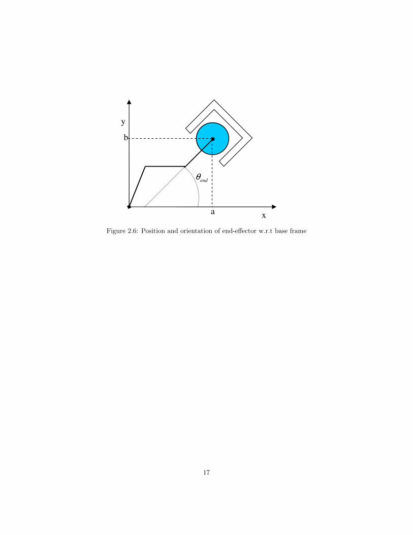
An example is given next. The end-effector must have a certain orientation andposition in order to move the wafer without colliding with the magazine (see figure2.6). The end-effector orientation and position with respect to the base frame canbe given as:
H =[
cos(θend) −sin(θend) asin(θend) cos(θend) b
]=
[r11 r12 xr21 r22 y
](2.11)
16
y
x a
b
endθ
Figure 2.6: Position and orientation of end-effector w.r.t base frame
17

18

3 Decoupling Control
In this chapter the contents of several scientific articles which claim to be able todecouple the system are mentioned briefly. Then the advantages and disadvantagesof each method are discussed such that a conclusion can be drawn.
3.1 Decoupling via Computed Torque Control
A well known method to decouple a n-link rigid robot is the computed torque con-troller (see Spong e.a., 2006). The idea of computed torque is to algebraicallytransform a system of equations describing the nonlinear robot dynamics into alinear system by compensating all the coupling nonlinearities in (2.2) by applying:
τ = M(q)u + h(q, q) (3.1)
If there was no uncertainty about the modelparameters and if there were no uncer-tain highfrequent dynamics (i.e. τv = 0), the dynamics would become:
M(q)q + h(q, q) = τ = M(q)u + h(q, q) (3.2)
and the system would thus be decoupled since q = u. The transfer function of thesystem after decoupling becomes Gii = diag( 1
s2 ). Now control input u containsa feedback correction term and an acceleration correction term in order to correctfor the acceleration perturbation caused at other joints:
u = qd − u∗ = qd −Kpe−Kde (3.3)
where Kp and Kd are diagonal positive definit matrices and e = qd − q and e =qd − q. Since the model based portion of the controller reduces the rigid bodydynamics of the robotic manipulator to a pair of independent unit inertia moments,the error driven portion is simplified to a pair of identical compensators designedfor a linear single degree of freedom (SDOF) system. The PD gains can be selectedusing a pole placement approach:
kp = ω2d, and kd = 2ξdωd (3.4)
with ωd the desired natural frequency of the closed loop system and ξd the dampingratio.
However, the system is subjected to uncertainties τv , e.g. due to friction
M(q)q + h(q, q)− τv = τ = M(q)u + h(q, q) (3.5)
and thus: q−M−1τv = u. Then the error dynamics finally become:
e + Kde + Kpe = M−1τv (3.6)
The presence of the uncertainties puts more restrictions on Kp and Kd since non-linear coupling between the error dynamics and the uncertainty limits the band-width of the system. Since the rigid body model is hardly an accurate description
19

of the real robot dynamics exactly, a more general transfer function can be consid-ered:
G(s) =
G1,1 · · · G1,n
.... . .
...Gn,1 · · · Gn,n
(3.7)
The crossterms represents interactions between the joints that remain after imper-fect compensation of the real robot dynamics. If the dynamic model matches thereal system accurate enough, then Gi,i dominates Gi.j and feedback control de-sign will be reduced to three single input single output (SISO) systems, which arehigher order dynamical systems with resonance and antiresonance frequencies.See the next figure for the control structure.
Trajectory planner
SCARA
u hMuτ += τ ( )hτMq −=−1
ɺɺ
Decoupling Controller
Outer Loop Controller
, ,ref ref refθ θ θɺ ɺɺ
,θ θɺ
,θ θɺ
Figure 3.1: Schematic overview of computed torque control
Stability Proof In order to prove the stability of the system under control, givenby the next equation, Lyapunov stability theorem is used.
Mq + h = τ = h + Mu = h + M(−Kve−Kpe) (3.8)Choose the positive definite Lyapunov function:
V =12qT q +
12qT Kpq (3.9)
Its derivative becomes then:
V = qT q + qT Kpq= qT (−Kve−Kpe) + qT Kpq= −qT Kvq− qT Kpq + qT Kpq, since qd,= qd = 0= −qT P0Kvq ≤ 0
(3.10)
In order to prove that the system will not sustain at somewhere q 6= qd, LaSalle’stheorem is used. Take V = 0 i.e. q = 0 and q = 0 and the error equation becomes:
Mq + h = h + M(−Kve−Kpe)Mq = M(−Kve−Kpe)
MKpe = 0(3.11)
20

and thus e = 0 since M and Kp are both nonzero. Thus it is proven that thecontrol system is global asymptotically stable.
Conclusion Using the the computed torque controller results in a system whichis decoupled and the dynamics after decoupling are linear if the model parametersare accurate and the system is subject to small perturbations. For this controller thefundamental equations are used to achieve modelbased decoupling. Therefore theinfluence of parameter error is minimal. But if the parameters are not estimatedvery accurately, the controller will generate the wrong torque which results in aworse performance and the system will not be decoupled and linear anymore. Inappendix G simulations are performed which show that for an error of 7 % in all theparameter mi, Li and Ii, the output of the other links is at least 8 dB smaller thanthe output of the actuated joint. This means that the system remains decoupledfor an error smaller than 7 %. But it is clear that in practice not only the modelparameters influence the decoupling, but other unmodeled effects such as friction,although small, will deteriorate the decoupling effect. Additionally, it is studiedwhat happens when the end-effector lifts a load. In this case the system will not bedecoupled even if a small load of 0.1 kg is lifted.
3.1.1 Adaptive Case
Since themodel parameters are not known exactly and since the parameters changewhen a load is lifted, an adaptive decoupling controller based on the computedtorque controller is studied. Consider the system under closed loop where M and hare terms of dynamic equation of the model containing the false model parameters:
M(q)q + h(q, q)− τv = τ = M(q)(qd −KDe−KP e) + h(q, q) (3.12)
which gives the error dynamics as:
e + KDe + KP e = M−1Y(q, q, q)a
where a = a− a , a is the estimate of the parameter vector a. Y a is the regressorform of the robot dynamics as mentioned in section 2.3. In state space the errordynamics are:
˙e = Ae + BΦa (3.13)
where e =[
ee
], A =
[0 I
−KP −KD
], B =
[0I
], Φ = M−1Y(q, q, q). Let
P be the unique symmetric, positive definit matrix, satisfying the matrix Lyapunovequation:
AT P + PA = −Q (3.14)
Using the Lyapunov function
21

V = eT Pe +12aT Γa (3.15)
Global convergence of the tracking error can be shown if we calculate V :
V = −eT Qe + aT{
ΦT BT Pe + Γˆa}
(3.16)
and choose the parameter update law as
ˆa = −Γ−1ΦT BT Pe (3.17)
where Γ is a constant, symmetric positive definite matrix. Now we get:
V = −eT Qe (3.18)
which shows that the position error converges to zero and the parameter estimationerror remains bounded.
Conclusion This adaptive decoupling controller contains two drawbacks for im-plementation on real systems. First of all, the inverse of the inertia term must becalculated online in order to calculate the update law. This will cost a lot of compu-tational burden. Secondly, the acceleration and velocity are needed for calculationof the regressor matrix Y. Since only position is measured, this signal has to bedifferentiated twice. This will lead to inaccurate and noisy signals.
3.2 Input-Output Linearization and Decoupling via Re-stricted State Feedback with Disturbance Rejection
In Tsirikos and Arvanitis (2000) an algebraic approach is treated to find a statefeedback controller which linearizes and decouples the system while disturbancetorques such as friction are rejected by this controller. In order to find a solution,several conditions which guarantee linearization, decoupling and disturbance re-jection, need to be fulfilled. This is called the disturbance rejection with simultane-ous I/O linearization and decoupling (DRLD) problem. A summary of the theoryof this method is given in appendix F. Next the theory is applied to the SCARA.After the system dynamics are written in the state space form, it becomes clearthat the DRLD problem can not be solved for this system, i.e. the conditions fordecoupling and disturbance rejection could not be fulfilled simultaneously. Finallyit is assumed that the system has no disturbances and the only possible solutionresults in a controller similar to the computed torque controller.
3.3 Decoupling Control including Motor Dynamics withDisturbance Decoupling
In Zhu e.a. (1993) a scheme for the decoupling control of robotic manipulatorsis proposed. Here the dynamic model includes the mechanical dynamics of the
22

links as well as the electrical dynamics of the joint motors, since in the case ofquick operation and especially for direct drive robots, actuator dynamics play animportant role in the overall robotic dynamics. Taking into account for these motordynamics will improve the performance of the robot. This control algorithm usesthese dynamics of the actuators in order to decouple the system. The resultingdecoupling controller is a simple algorithm which decouples the system into threeSISO systems of the form 1
s2 . Uncertain effect such as frictional effects, modelperturbations and external disturbances are attenuated by the uncertainty-rejectingmechanism.
In simulations this scheme gives excellent performance even under the influ-ence of large internal parameter variation and external disturbance. But for thisalgorithm the states of the system i, q, q,
...q are needed, which can limit practical
implementation on a real system. Additonally this algortihm is derived for a directdrive actuator with DC actuators with voltage as input. The SCARA considered inthis work contains AC actuators with current as input. As mentioned in the article,this algorithm can also be revised for other kind of actuators. However, no otherliterature is found for this algorithm, for its implementation and neither for itsperformance on real systems.
3.4 Decoupling Controller based on LS-SVM
This method which is proposed byWen e.a. (2006) is based on the idea to learn theinverse dynamics of the system. Connecting this inverse system to the real systemwill lead to a decoupled system. The basic idea is to send a random signal to theinput of the system and measure the output. Then the system is learned offline byuse of Least Square Support Vector Machine (LS-SVM). The inverse dynamics arelearned since the input and output of the system will behave as output and inputrespectively. In order to remain stable subsystems, the inputdata to the LS-SVMwill be transformed with use of pole placement.
Because this is a data-based method to decouple the system, the robot dynamicsneed not to be calculated. Therefore this method can be very efficient. Use of LS-SVM is more practical then standard SVM since no number of hidden units haveto be determined for the controller. Secondly no centers have to be specified forthe Gaussian kernel when applying Mercer’s condition, and fewer parameters haveto be described via the training process. Although simulation results of a simplenonlinear coupled system show good performance, its application on real systemsstill needs further study.
3.5 Conclusion
In this chapter several decoupling methods are studied and compared. Three mod-elbased decoupling controllers are described and one data-based decoupling con-troller. After the advantages and disadvantages of each decoupling method arestudied, a comparison is made. The computed torque control decouples the sys-tem if the model parameters are accurate enough and the error will theoreticallyconverge to zero for a pd design using poles placement. Then the problem reduces
23

to the linear case. It is studied that an error of all the parameters mi, Li and Ii
less than 7 % will result in an worst case decoupling of 8 dB. But it is clear thatin practice not only the model parameters influence the decoupling, but other un-modeled effects such as friction, although small, will deteriorate the decouplingeffect. Additionally, it is studied what happens when the end-effector lifts a load. Inthis case the system will not be decoupled even if a small load of 0.1 kg is lifted andtherefore the parameters of the end-effector need to be updated. Additionally, anadaptive version of the computed torque controller is studied. It is concluded thatpractical implementation is limited due to the need of measuring the acceleration.Next the robot dynamics are written in state space form in order to find an algebraicsolution for decoupling and linearization of the system while disturbances are re-jected simultaneously. The algorithm uses the restricted state feedback. However,no disturbance rejecting mechanism can be achieved for the dynamic equations ofthis SCARA. Without disturbance decoupling, the resulting decoupling controlleris the same as the computed torque controller. Next another model based decou-pling controller is mentioned which accounts for the dynamic interaction of actu-ator and link in order to improve performance and to improve decoupling in caseof disturbances and model parameter errors. This algortihm includes also a dis-turbance rejection mechanism which performs well according to the simulationresults. However, no literature can be found with the practical implementation ofthis algorithm and since the third order derivative of q is required it is doubtfulwhether this method will perform well. Furthermore, this algorithm is derived fordc actuators with voltage as input. Finally, a databased decoupling mechanism isstudied which uses LS-SVM to learn the inverse dynamics. This method mightoffer a good performance and is an efficient method since it is databased. Butits application on real (robotic) systems still needs further study. Finally it can beconcluded that the computed torque controller is most suitable to decouple the sys-tem due to practical limitations of the other methods. The only way to succeed indecoupling is to acquire a model as accurate as possible.
24

4 Feedback Control Design for the Decoupled Sys-tem
If the model used in the computed-torque controller is accurate enough, the re-maining dynamics are mostly decoupled and linear dynamics. In that case severalSISO feedback methods can be used. First a few methods to identify the dynam-ics after decoupling are discussed. Then some outerloop controllers are selected,followed by simulations to study the performance.
4.1 Dynamics after Decoupling
Since the system is decoupled for a parameter error of less then 7%, a SISO con-troller can be designed for the spectrum of each decoupled joint. The high frequentdynamics which are not compensated with the rigid-body dynamic model, influ-ence feasible levels of the motion control performance and robustness. Thereforeit is worthwhile spending additional effort on determining them (Kostic, 2004).Three methods to identify the dynamics after decoupling are described next.
Shifting Open Loop Dynamics The first method is to shift the open loop sys-tem dynamics such that the rigid body dynamicsmatch the decoupled dynamics 1
s2 .Before doing this, the discrete velocity spectrum has to be changed into a positionspectrum, as is explained in appendix L. A disadvantage of this method is that oneis not sure if this represents the real dynamics since the resonance may changeafter decoupling. When the performance of the outerloop controller is assessed insimulations this method is used. To be sure what the remaining dynamics are, anidentification test on the real system after decoupling has to be done.
Closed Loop Identification Since the MIMO coupled system is decoupledto three SISO systems, one can use closed loop identification methods which areoften used for SISO systems. A method which does not result in a biased identifi-cation due to mutually correlated disturbance components of the measured signalsis explained next. White noise has to be inserted between the PD controller and thedecoupling controller, such that the input to the decoupling controller becomes:
u = Kpe + Kde + v(t) (4.1)
where v(t) is the external excitation which is not correlated to any disturbances ofu. This circumvents the problem of biased identification. Then the sensitivity canbe determined by:
S =v
u=
11 + CG
(4.2)
Since a PD controller is used, the dynamics can be calculated according to:
C(ω) = ωkd,i + kp,i
Gi.i(ω) = 1/S(ω)−1C(ω)
(4.3)
25

For each plant Gii this identification can be performed for several configurations.The other joints are therefore not allowed to move and thus a high PD gain must beapplied to these joints. The controller of the joint whose spectrum has to be deter-mined, must have a small PD gain since the feedback controller strongly attenuatesharmonic components of ui within the bandwidth. This reduces the signal to noiseratio for these harmonics and in turn leads to poor coherence. Since the firmwareof the system does not support a white noise identification the open loop identifi-cation is used.
Open Loop Identification An open loop identifcation of the system after de-coupling can be performed using white noise or a swept sine. The input and outputof the sytem can be collected and the system’s transferfunction can be determined.One drawback of this method is that the system during open loop identification isnot necessarily stable and it is hard to let the system in a certain configuration. Insimulation these two problem are solved by decreasing the input amplitude. How-ever in the real system this will result in a noisy measurement. In order to do astable open loop identification after decoupling, one must compensate for inertiaonly. The joints of the other two links must be clamped and their actuator mustbe disabled and therefore the terms h(q, q) + M(q)q can be disabled since theywill be equal to zero. This means that only inertia compensation is enabled. Mini-mal adjustments in the firmware of the SCARA have to be done for the openloopidentification using swept sine.
4.2 Outer Loop Controller
Once the dynamics after decoupling are identified, one can design different outerloop controllers. Since the remaining plant dynamics are captured, a PD controllercan be designed in frequency domain by performing loop-shaping according to thestandard design rules:
1. stabilize plant Gii
2. ensure high open-loop gain CG, with the largest possible cross-over fre-quency (bandwidth).
3. allow maximal peaking in the sensitivity function S of 6 dB
4. minimize the influence of unmodelled dynamics and disturbances on themotion control performance
Several control methods applied to direct drive robotics can be found in literature inorder to handle with the high frequent resonances, such as robust control and ILC.Other approaches such as low-pass filter are not effective since they introduce am-plitude distortion and destabilizing phase delay. Another approach is to use bandreject filters, but this is not suitable for applications where the resonance conditionsshift during operation, caused by wear and tear or production inconsistency. Next,a method is described which is found to be usefull in case of mass-production.
26

4.2.1 Observer-Corrector Control Design
In section 3.1 it is assumed that the full state information, that is position and ve-locity, is available in order to calculate the computed torque controller. In practice,velocity is not measured but differentiated from the measured position. Since thissignal contains high frequent noise an observer will be used to estimate the ve-locity. In literature many observers for this problem can be found, for instancein Berghuis (1993a), Berghuis et al. (1992b). In Hosek (2003), the fundamentalidea is to synthesize a wrong observed velocity (since a linear observer is used andthe system is not perfect linear due to model inaccuracies) with the lowfrequentcontent of the differentiated velocity. Then the substituted feedback signal reflectsthe dominant dynamics essential for operation of the system subject to control butdoes not include the undesirable higher order dynamic effects.
PD Control by Pole-Placement Since the model based portion of the con-troller reduces the rigid body dynamics of the robotic manipulator to a pair of in-dependent unit inertia moments, the error driven portion is simplified to a pairof identical compensators designed for a linear single degree of freedom (SDOF)system. The PD gains can be selected using a pole placement approach:
kp = ω2d, and kd = 2ξdωd (4.4)
with ωd the desired natural frequency of the closed loop system and ξd the dampingratio. As mentioned before ωd cannot be chosen too high since the higher orderdynamics will make the system unstable.
Observer Since the model-based portion of the controller reduces the rigid-bodydynamics of the robot to a pair of independent unit inertia moments q = u, it isconvenient to partition the state observer into three identical sections designed fora simple SDOF system. For each joint, the remaining dynamics can be written instate space form as:
x = Ax + Bu =[
0 10 0
]x +
[01
]u (4.5)
with the states x =[
ϑ ϑ]T
and u the input to the linearized system (see figure4.1).
The state of the system can be estimated by making use of the observer: ˆx =Ax + Bu. The difference between the real output and the estimated output, i.e.ϑ − Cx, is a measure of the quality of the observed state. The full observer isobtained when this quality measure is fed back to the observer with the observer
gain matrix K =[
k1 k2
]T:
ˆx = Ax + Bu + K(ϑ− Cx)= Ax + Bu + Kϑ−KCx
= Ax + Bu +[
k1
k2
]ϑ−
[k1 0k2 0
]x
(4.6)
27

The observer design problem reduces to find a suitable gain K such that the ob-server gets suitable dynamic properties. Consider the reconstruction error xerr =x− x and the differential equation of the error dynamics becomes:
xerr = x− ˆx = Ax + Bu−Ax−Bu−Kϑ + KCx= A(x− x)−KC(x− x) = (A−KC) xerr
(4.7)
The eigenvalues determine the observer properties and are given by: λ1,2 = −k1±√
k21+4k2
2, which give the solution for gains k1 = 2ξoωo and k2 = ω2
o . Then each of the ob-servers operates based on the following state equations:[
xi1
xi2
]=
[−2ξoωo 1−ω2
o 0
] [xi1
xi2
]+
[2ξoωo 0
ω2o 1
] [ϑi
ui
](4.8)
where xi1 and xi2 are the observed states (angular position and velocity) of jointi and ωo and ξ0 stands for the natural frequency and damping ratio associatedwith the dynamics of the state observer. The choice of observer dynamics is atrade off between reconstruction speed (speed of decay of reconstruction error)and sensitivity to measurement noise. The observer poles (eigenvalues) must befaster that the closed loop system poles, because it is then able to follow the closedloop dynamics. Too fast an observer will lead to sensitivity to measurement noisesince the observer will be able to follow higher frequencies than those of interest toclosed loop control.
Corrector The output of the plant consist of a low and a high frequent content:
ϑ(t) = ϑd(t) + ϑh(t) (4.9)
where yd refers to the dominant dynamics of the plant and yh corresponds to thehigher order dynamics of the plant. The accuracy of the estimated output of theplant is limited due to observation errors (ye(t)) which typically result from modelparameter errors in the decoupling controller and is thus of low-frequent content.So the output of the state observer can be written as:
ϑo(t) = ϑd(t) + ϑe(t) (4.10)
Subtracting (4.10) from (4.9) gives:
ϑ(t)− ϑo(t) = ϑh(t)− ϑe(t) (4.11)
In order to get ye from this signal, a second order lowpass filter is used, which iscalculated with:
Gc(s) =ω2
c
s2 + 2ξcωcs + ω2c
(4.12)
where ωc is the cut-off frequency and for the damping ratio ξc = 1/√
2, the filterprovides attenuation of 3 dB at the frequency of ωc. Since the corrector filter is
28

linear, the path from input to output of the corrector can be observed in Laplacedomain:
ϑc = Gc(s)[ϑh(s)− ϑe(s)
]= Gc(s)ϑh(s)−Gc(s)ϑe(s) (4.13)
and since the filter attenuates the higher order dynamics, the output of the correctorbecomes:
ϑc(s) ≈ −ϑe(s) , or ϑc(t) ≈ −ϑe(t) (4.14)
Then this signal is added to the observed signal, such that the substitute feedbacksignal becomes:
ϑs(t) = ϑo(t)− ϑc(t) = ϑd(t) (4.15)
See figure below for the control structure.
Trajectory planner
SCARA
u posref accref hMuτ +=
ref
C
acc
eKeK dp
+
+= ɺ τ ( )hτMq −=−1
ɺɺ
Decoupling Control
State observer
Corrector filter
d/dt q
qɺ
+ - o
qɺ
+ + s
qɺ
Figure 4.1: Control structure for observer-corrector
29

4.3 Simulation Results
At first the control gains are tuned for the PD, PD + lowpass and PD + observeraccording to the loop shaping rules. The achieved control gains are given in appen-dix I where it is shown that for a PD controller low gains are achieved compared toa PD controller combined with a lowpass filter or an observer. In order to predictthe performance of all controllers on the real system, a time motion is simulatedfor the MIMO model. For the parameters of the decoupling controller, the worstcase parameter error of 7 % is used. A movement of pi radians of the shoulderis performed while the other joints stay in the extended configuration. The maxi-mal allowed velocity and acceleration is 10 rad/s and 10 rad/s2 resp. In table 4.1one can see that the performance of the observer-corrector structure is much betterthan when a lowpass filter is used. In figure 4.2 the raw velocities are comparedto the velocity after filtering, the observed velocity corrected signal, the substitutesignal represents the real signal quite accurate. After all it can be concluded thatthe performance of the controllers for the simulated system is acceptable. But itmust be mentioned that the remaining high frequent resonances are not necessar-ily the same as the shifted dynamics and it is not known if the model parametersare within 7 %. Therefore it is chosen to get the dynamics after decoupling on thereal system before implementing these controllers on the system.
error [rad] Observer-corrector Lowpassshoulder 1e-4 5e-3elbow 1e-4 4e-4wrist 1e-4 1.2e-3
Table 4.1: Maximal error for worst case decoupling
30

0.5 1 1.5 2 2.5-0.02
-0.01
0
0.01
0.02
0.5 1 1.5 2 2.5-0.04
-0.02
0
0.02
0.04
0.5 1 1.5 2 2.5-2
0
2
4
6
raw
observer
observer-corrector
lowpass
1.1 1.15 1.2 1.25 1.3
4.25
4.3
4.35
4.4
4.45
4.5
velo
city [
rad/s
ec]
time [sec]
Figure 4.2: a: Joint velocity versus time. b: First subfigure zoomed in
4.4 Conclusion
In order to design a controller with good performance, the dynamics after de-coupling need to be identified. Therefore three methods are described with their(dis)advantages. Next several controllers are compared to see which is most suitedfor this application. Use of bandlimited filters are not suitable in case of massproduction. Therefore a lowpass filter can be applied before the first resonance.However this will lead to a large decrease of the control gains, since the lowpasswill introduce a lot of phase delay. Nevertheless, this structure is still better thanwithout a lowpass filter. Another structure is studied, which observes the veloc-ity with linear observers. Since the decoupled system is not perfectly linear dueto inaccurate decoupling, a corrector filter is implemented in the structure. This
31

structure effectively eliminates destabilizing effects of the undesirable higher orderdynamics
One can conclude that this control design strategy in comparison to a commonpd or a pd plus lowpass provides improved performance, increased stability mar-gin and added robustness against variations in system parameters in case of massproduction. An improvement of factor 10 compared to pd plus lowpass is achieved.Finally it must be mentioned that many other observers can be found in literaturewhich might estimate the state better than the linear observers used in this work. Afeedback linearizing controller-observer system can be found in Berghuis (1993a)and Berghuis et al. (1992b). Additionally, many other outerloop controllers can beused such as robust control (Kostic, 2004).
32

5 Implementation
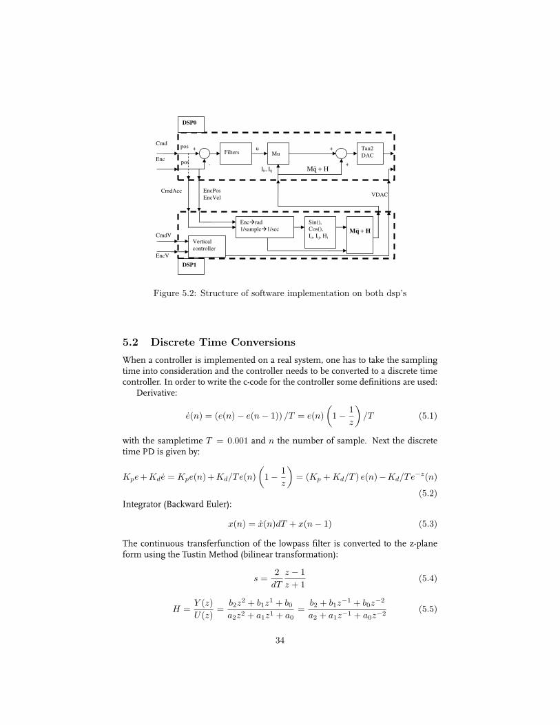
5.1 Implementation on a SCARA Platform
The motion platform of the SCARA consists of three digital signal processors(DSP) and two field programmable gate array’s (FPGA), see figure 5.1. The com-mand signal of each joint comes from the high level PC and is sent via the FPGA1to both DSP’s. The encoder signals from the feedback devices are fed throughFPGA2 and are sent to the DSP’s. On DSP0 the servo controllers of the three rota-tional axes are implemented in c-language. On DSP1 the control of the vertical axisand the calculation of the decoupling controller is implemented. The structure ofthe implemented controllers is divided over two DSP’s, since the controllers wereinitial designed for 4 kHz and the calculation time becomes more critical then.The decoupling structure is implemented such that minimum changes have to bemade. The structure is visualized in figure 5.2.
SEW enc
SEWV DAC SEW cmd
V cmd
SEWV
cmd
Vbrake DAC
V enc
SEW cmd
SEW enc
V DAC
HqM +ɺɺ
Z
fpga1 fpga2
DSP3
DSP1
DSP0
PCI
To Other XY controller
To BQM controller
8x 16 bit ENCs 12x 16 bit Dac 16 Inputs 16 Outputs 8 ADC’s S I/O (32bits)
Figure 5.1: SCARA platform
33
DSP1
Cmd
Enc
HqM +ɺɺ
Filters u
Mu +
-
+
+
Tau2 DAC
pos
pos
EncPos EncVel
CmdAcc
CmdV
EncV
Vertical controller
Enc�rad 1/sample�1/sec
Sin(), Cos(), Iii, Iij, Hi
HqM +ɺɺ
DSP0
VDAC
Iii, Iij
Figure 5.2: Structure of software implementation on both dsp’s
5.2 Discrete Time Conversions
When a controller is implemented on a real system, one has to take the samplingtime into consideration and the controller needs to be converted to a discrete timecontroller. In order to write the c-code for the controller some definitions are used:
Derivative:
e(n) = (e(n)− e(n− 1)) /T = e(n)(
1− 1z
)/T (5.1)
with the sampletime T = 0.001 and n the number of sample. Next the discretetime PD is given by:
Kpe+Kde = Kpe(n)+Kd/Te(n)(
1− 1z
)= (Kp + Kd/T ) e(n)−Kd/Te−z(n)
(5.2)Integrator (Backward Euler):
x(n) = x(n)dT + x(n− 1) (5.3)
The continuous transferfunction of the lowpass filter is converted to the z-planeform using the Tustin Method (bilinear transformation):
s =2
dT
z − 1z + 1
(5.4)
H =Y (z)U(z)
=b2z
2 + b1z1 + b0
a2z2 + a1z1 + a0=
b2 + b1z−1 + b0z
−2
a2 + a1z−1 + a0z−2(5.5)
34

Using the time shifting property, the output of the discrete filter can be calculated:
x[n− k] = z−kX(z) (5.6)
yna2 = u(n)b2 + u(n− 1)b1 + u(n− 2)b0 − y(n− 1)a1 − y(n− 2)a0 (5.7)
35

36
6 Experimental Results
6.1 Dynamics after Decoupling
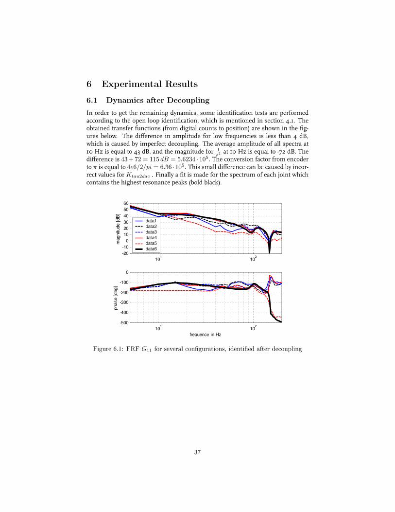
In order to get the remaining dynamics, some identification tests are performedaccording to the open loop identification, which is mentioned in section 4.1. Theobtained transfer functions (from digital counts to position) are shown in the fig-ures below. The difference in amplitude for low frequencies is less than 4 dB,which is caused by imperfect decoupling. The average amplitude of all spectra at10 Hz is equal to 43 dB. and the magnitude for 1
s2 at 10 Hz is equal to -72 dB. Thedifference is 43+72 = 115 dB = 5.6234 · 105. The conversion factor from encoderto π is equal to 4e6/2/pi = 6.36 ·105. This small difference can be caused by incor-rect values for Ktau2dac . Finally a fit is made for the spectrum of each joint whichcontains the highest resonance peaks (bold black).
101
102
-20
-10
0
10
20
30
40
50
60
magnitude [
dB
]
shoulder spectra
data1
data2
data3
data4
data5
data6
101
102
-500
-400
-300
-200
-100
0
phase [
deg]
frequency in Hz
Figure 6.1: FRF G11 for several configurations, identified after decoupling
37

101
102
-20
0
20
40
60
magnitude [
dB
]
elbow spectra after decoupling
data1
data2
data3
data4
data5
Fit
101
102
-300
-250
-200
-150
-100
-50
phase [
deg]
frequency in Hz
Figure 6.2: FRF G22 for several configurations, identified after decoupling
101
102
-20
0
20
40
60
magnitude [
dB
]
wrist spectra decoupled
data1
data2
data3
Fit
101
102
-300
-250
-200
-150
-100
phase [
deg]
frequency in Hz
Figure 6.3: FRF G33 for several configurations, identified after decoupling
38

6.2 Control Design
A PD controller is designed using DIET while considering the loop shaping rulesgiven in section 4.2. This results in the gains given in table 6.1. The cutoff frequen-cies of the lowpass filters are set to 120 Hz with a damping of 0.7 (see appendixJ). The open loop spectrum CG for all joints are given in figure 6.4. Finally thegains are tuned on the real system, resulting in the new PD gains which are alsogiven in the table. A motion from folded to extended configuration is shown infigure 6.5. At the final stage there is a vibration of the wrist. This is caused by thestatic integrator which is enabled at the time when the command velocity is equalto zero. In order to reduce this vibration, the integrator constant of the wrist hasbeen reduced to a value of 0.0001.
Figure 6.4: Open Loop CG
PD PD tuned on systemgain zero gain zero static integrator
Shoulder 0.005 20 0.0125 20 0.000029Elbow 0.003 15 0.01 15 0.000025Wrist 0.01 30 0.0125 30 0.0001
Table 6.1: Controller gains, initial and after tuning on system
39

0 1000 2000 3000 4000 5000 6000 7000 8000 9000 10000-0.5
0
0.5
1
1.5
2
2.5x 10
6
time
encoders
Scmd
Senc
Ecmd
Eenc
Wcmd
Wenc
6400 6500 6600 6700 6800 6900 7000 7100
time
Scmd
Senc
Ecmd
Eenc
Wcmd
Wenc
Figure 6.5: Movement of pi radians for all joints simultaneously
6.3 Experimental Results
First several tests are performed to find the maximal velocity and acceleration. Forthe movement from folded to extended configuration a maximal velocity and accel-eration of 16 rad/s and 16 rad/s2 can be achieved.
First the influence ofKtau2dac is studied. The different gains are shown in table6.2. The first values are calculated according to (2.8). The next values are obtainedby tuning in an earlier stage of the control design. Then the values are shown whichare obtained by measurement. In order to compare the different constants, severalmotions are performed with a maximal allowed velocity and acceleration of 10m/s,10m/s2 respectively. In figure 6.6 several motions are visualized. For motion 1 to6 only one axis is moved individually. For motion 7 and 8 all axes are moved simul-taneously. The maximal dynamic error is a measure to quantify the decoupling.For each motion, the average maximal error of two motions is calculated which isshown in appendix K. The decoupling effect is studied by comparing the average ofthe error of all motions of each joint. For the shoulder and elbow best decoupling isobtained with the measured Ktau2dac, but for the wrist larger errors are obtained.The dac-torque measurement of the wrist was less accurate since lower torque isapplied in order to prevent a cutoff. Therefore it is chosen to use the tuned value
40

for the wrist. The mean value of all motions for each joint is calculated and bestperformance is achieved for Ktau2dac = [k1; k2; k3] = [131; 282; 356], see table 6.3.
The model parameters which are calculated by making a fit through the spec-trum (mentioned in section 2.3), are compared to the model parameters obtainedwith Solid Edge. In appendix K the results are shown and in the table 6.3 the av-erage maximal errors are shown. A minimal error is obtained when the modelparameters are used which are obtained by fitting the spectra.
Next the influence of large parameter errors is studied. In this case the parame-ters from prototype one are used. This prototype does not have any clamps buildin. Besides that, for the wrist the parameters are calculated in case of transportinga wafer. As expected and as shown in table 6.3 the error becomes much larger, dueto wrong torque calculation.
Finally the performance of the final controller is investigated and is shown intable 6.4. When the wrist is moved individually, decoupling is achieved. Howeverthis is also the case when no decoupling controller is used. When the elbow ismoved, the least amplitude difference between joint two and one of the other jointsis equal to -8 dB and -11 dB, for motion three and four respectively. Compared tono decoupling controller shows -3 dB and -11 dB (see Appendix B). So only motionthree shows improvements regarding decoupling. When the shoulder is movedin the folded configuration, it causes an error for the wrist of similar magnitude.When the shoulder is moved in the extended configuration, it causes an error forthe elbow which is a factor two larger. The same coupling is shown when no de-coupling controller is used. This indicates that no perfect decoupling is achieved.Motion 7 shows the largest error. This motion can be considered as the most crit-ical since the centrifugal and Coriolis torques play a large role at the moment thesystem is least decoupled. A maximal dynamic error of less then 4000 encoderscan be observed for the elbow. This dynamic error is equal to 0.006 rad. In figure6.7 the position and error of motion 8 are plotted.
The setling time is defined as the time at which the command velocity becomeszero until the time when the error is within a specified encoder value. This encodervalue is set to 50 encoders which is equal to 8 · 10−5rad. In table 4.1 the setlingtime for each motion is shown. The setling time of the elbow is largest, since thisjoint contains the largest dynamic error due to lower gains and due to the fact thatthe elbow is most disturbed by the other two joints. Another cause for the highersetling time is that the static integrator of the elbow is smallest and is a factor 4smaller than the wrist.
41

Shoulder
Elbow
Wrist
All
Extended configuration
Folded Configuration
1 2
4 3
5 6
7 8
shoulder elbow wrist
Figure 6.6: Performed motions
Ktau2dac S E Wcalculated 104 256 339
tuned 118 292 356measured 131 283 408
final 131 283 356
Table 6.2: Relationship between input (digital counts) and output (torque)
Ktau2dac tuned measured finalMax dyn. error [counts] 305 788 1088 287 762 991 293 769 983
Ktau2dac final parameters S.E. Parameters FitMax dyn. error [counts] 305 788 1088 287 762 991
Ktau2dac tuned Parameters Fit parameters SE prototype1 with waferMax dyn. error [counts] 376 829 941 485 790 1306
Table 6.3: Influence parameter change and Ktau2dac
42

Figure 6.7: Position and error as function of time (motion 8)
Max. dyn error [enc] Setling time [msec]S E W S E W
1 137 199 845 1 1 2513 188 852 350 1 531 2854 202 709 171 14 742 1055 350 727 479 1 879 3786 373 59 362 92 1 1087 622 2433 3908 302 756 2868 190 361 506 265 686 293
Table 6.4: Maximal dynamic error and setling time for the defined motions
43

6.4 Conclusion
First the dynamics after inertia compensation for several configurations are identi-fied and a fit is made for the most critical configuration. Next a PD controller foreach joint is designed using Diet. These controllers are tuned on the real system.The influence of Ktau2dac is studied as well as the performance if the modelpa-rameters from Solid Edge are used or if they are obtained by making a fit of thespectrum. It appears that the Ktau2dac measured on the real system are most ac-curate. However this depends on how accurate the measurement is since the forceis tried to keep at a constant value manually. Therefore further improvement canbe achieved when an electronic forcegenerator is used and this signal is captured.Using the modelparameters obtained by fitting the spectra results in better perfor-mance. But even for large parameter variation, the controller still works, but withlarge dynamic error. Finally the performance of the final controller is assessed. Itcan be concluded that no decoupling is achieved when moving the shoulder, sincethe other joints have larger error for some configurations. This is caused since thedecoupling controller only decouples for the rigid body dynamics and not for thehigher frequent resonances. However good performance is achieved with a maxi-mal dynamic error of less than 0.006 rad when all axes are moved from folded toextended configuration. Another performance indicator is the setling time, whichis defined as the time from when the command velocity is zero until the error issmaller than 8 · 10−5rad. The elbow has largest setling time which is less than 0.8sec. In order to improve the performance, the static integrator can be increased.More improvements can be achieved if the observer-corrector structure is imple-mented or when advanced robust controllers are implemented.
44

7 Adaptive Control Design for Vertical Stage
As mentioned in section 3.1 the system will not be decoupled in the case a load islifted. Therefore the parameters of the wrist have to be updated during operation.Several options are given. Firstly, if the payload is known in advance, the parame-ters can be changed when a wafer mapping sensor notices a wafer. If no sensoris available for detecting the wafer, the parameters can be updated if the system isable to know when it lifts a wafer, which can be implemented in the trajectory plan-ner. Another option is to use the vertical stage to estimate the mass of the waferusing adaptive control. This will be tested in this chapter. The parameters will beupdated according to the method mentioned in section G.2.
7.1 modeling
The model of the vertical axis is assumed to be of the form:
mz = u−mg − Ff (7.1)
where g is the gravity and Ff is the force due to friction. u is the input force tothe motor. The relation between digital counts to the driver and generated forceis determined when the system is in closed loop and when it is not moving. Thegenerated force compensates for the gravity force and thus m · g = 20.5 · 9.81 =kdac2force · DAC. This results in kdac2force = 1. Next the friction parametersare determined by moving the vertical axis with a constant velocity and the averageDAC output is calculated. The obtained friction curve and the fitted model areshown in the figure below. The peak in the friction force at low velocities is due tothe Stribeck effect. A fit is made using a simplified friction model:
Ff = fc · sign(z) + fv · z (7.2)
Here are fc and fv Coulombs and viscous friction respectively. For a good fit theirvalues are 100 and 1200 respectively.
45

-0.08 -0.06 -0.04 -0.02 0 0.02 0.04 0.06 0.08-200
-150
-100
-50
0
50
100
150
200
250
velocity [m/s]
DA
C
Figure 7.1: Experimental friction data (blue) and simplified model (dotted)
7.2 Adaptive Control
Many adaptive control methods can be found in literature. Two well known con-cepts are Model Reference Adaptive Control (MRAC) and Self-tuning control (Slo-tine, 1991). Both concepts use a servo controller which contains the adjustableparameters. MRAC updates the model parameters based on the error between thereference position and velocity, generated by the reference model, and the mea-sured position and velocity. The objective of the adaptation is to converge the track-ing error to zero. Self-tuning control works as follows: The parameter estimatorcollects the input and output of the plant and an input-ouput fit is made based ona least-square method. When the mass is not moving the digital counts was ina range of 197 to 214 for different tests. Therefore it is expected that self-tuningcontrol will not be able to estimate the mass fast and accurate and thus MRAC ischosen and will be further explained next. The model is assumed to be of the formof (7.1) and (7.2). If the mass and friction are known exactly, the next feedbackcontrol can be used to achieve perfect tracking:
u = m(zref + g − 2λe− λ2e
)+ fcsign(z) + fv z (7.3)
where λ is a positive definit control parameter. Using this controller will lead toexponential convergent error dynamics:
e + 2λe + λ2e = 0
where e = z − zref .However, the mass m and friction parameters fc and fv are not known exactly.
Therefore m, fc and fv are used instead, which leads to the error dynamics:
46

ms + λms = φ1v1 + φ2v2 + φ3v3 (7.4)
Here is s the combined tracking error, v the signal quantity and φi is the differencebetween estimated parameter and the true value:
s = e + λe (7.5)
v =
v1
v2
v3
=
zm + g − 2λe− λ2esign(z)
z
(7.6)
φ =
m−m
fc − fc
fv − fv
(7.7)
Next the update law of the mass is chosen to be:
˙φ = −γvs (7.8)
where γ =
γ1
γ2
γ3
, which is called the learning rate.
Together with this update law, the stability can be proven by Lyapunov theorem.The positive definit Lyapunov function is then:
V = ms2 +1γ
φ2 (7.9)
And its derivative becomes:
V = mss + 1γ φ
˙φ
= mss + 1γ φ
( ˙φ− φ
), φ = 0 since parameters are constant
= mss + 1γ φ (−γvs)
= mss + 1γ φ (−γv1s) , if γ2 = γ3 = 0, i.e. no adaption for friction
= mss− φ1v1s− φ2v2s− φ3v3s
= mss− (ms + λms) s +(φ2v2 + φ3v3
)s− φ2v2s− φ3v3s
= −λms2 ≤ 0
(7.10)
Since V is smaller than or equal to zero, stability is proven. In order to provethat s converges to zero, Barbalat’s lemma is used and the second derivative of theLyapunov function is:
V = −2λms(φv − λs
)(7.11)
47

Since s and φ are shown to be bounded earlier and since V is bounded, itmeans that V is continuous in time and s goes to zero for t goes to infinity. Sinces converges to zero, e and e converge both to zero.
Next parameter convergence will be discussed. From (7.8) it follows that ˙φ
becomes zero and thus φ becomes constant. Differentation of (7.4) and since s and˙φ are zero for t →∞ finally gives: 0 = φv. So convergence of parameter estimationwill only be guaranteed if v is persistently exciting. The schematic structure is givenin the figure below:
Plant 2ˆ ( 2 )
* ( ) *
ref
c
u m z g e e
f sign z fv z
λ λ= + − − +
+
ɺɺɺ
ɺ ɺ
ees λ+= ɺ 2
1 2ref
v z g e eλ λ= + − −ɺɺɺ
svm 11ˆ γ−=ɺ
,z zɺ
, ,ref ref ref
z z zɺ ɺɺ
qmee ɺɺ ,ˆ,,
Feedback controller
Parameter estimator
Figure 7.2: Schematic structure of MRAC
7.3 Simulation Results
Several simulations are done to study the adaptive control. The maximal trackingerror can be increased/decreased by adjusting the control parameter λ. Increasingthe learning rate, γ, results in faster adaptation and therefore smaller tracking er-rors. However, the estimation becomes also more sensitive for noise. For a controlparameter λ = 10 and γ = 30, the maximal error is then 0.006 m for a stepsize of0.01 m. The estimated mass converges to the real value of 20.5 kg. For λ = 200leads to the wrong estimation of the mass since the tracking error is kept too small.The system’s mass (20.5 kg), is estimated by 21.3 kg. In case of a payload of 0.2 kgthe mass estimated is 21.5 kg. This means that the mass of the payload still can beestimated accurately. It can be concluded that tuning the parameters γ and λ is atradeoff between small tracking error and fast and accurate estimation.
To study the influence of friction some other simulations are done. In figure7.3 the tracking error and the mass estimation are shown for three simulations
48
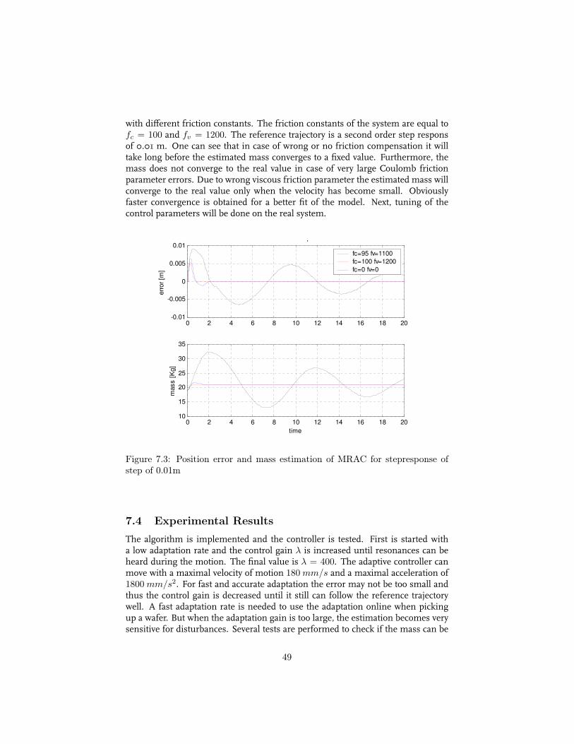
with different friction constants. The friction constants of the system are equal tofc = 100 and fv = 1200. The reference trajectory is a second order step responsof 0.01 m. One can see that in case of wrong or no friction compensation it willtake long before the estimated mass converges to a fixed value. Furthermore, themass does not converge to the real value in case of very large Coulomb frictionparameter errors. Due to wrong viscous friction parameter the estimated mass willconverge to the real value only when the velocity has become small. Obviouslyfaster convergence is obtained for a better fit of the model. Next, tuning of thecontrol parameters will be done on the real system.
0 2 4 6 8 10 12 14 16 18 20-0.01
-0.005
0
0.005
0.01influence of friction parameters
err
or
[m]
fc=95 fv=1100
fc=100 fv=1200
fc=0 fv=0
0 2 4 6 8 10 12 14 16 18 2010
15
20
25
30
35
time
mass [
Kg]
Figure 7.3: Position error and mass estimation of MRAC for stepresponse ofstep of 0.01m
7.4 Experimental Results
The algorithm is implemented and the controller is tested. First is started witha low adaptation rate and the control gain λ is increased until resonances can beheard during the motion. The final value is λ = 400. The adaptive controller canmove with a maximal velocity of motion 180 mm/s and a maximal acceleration of1800 mm/s2. For fast and accurate adaptation the error may not be too small andthus the control gain is decreased until it still can follow the reference trajectorywell. A fast adaptation rate is needed to use the adaptation online when pickingup a wafer. But when the adaptation gain is too large, the estimation becomes verysensitive for disturbances. Several tests are performed to check if the mass can be
49

estimated accurately for different values of γ. Finally γ = 200 and λ = 200 areused. The results are shown in the table 7.1. The mass is not estimated with anyrepeatability. The avarage of the estimated payload is equal to 2.2 kg. The largechanges in estimation are caused since the friction model is not accurate enough.Including the Stribeck effect into the friction model will improve the mass estima-tion. The Lugre friction model can be used herefore. However, since the friction isnot constant at different positions, the mass of a wafer can not be estimated accu-rately enough, but the mass of a magazine might be estimated roughly, such thatdecoupling of the three coupled links can be improved. For now the adaptation rateis set to zero with initial estimation of 21 kg and the control parameterλ = 400.
Motion no payload payload(2.3Kg)1 16.5 18.12 16.4 20.43 19.1 19.84 18.0 19.85 18.4 16.86 16.8 227 16.6 20.1
Mean 17.4 19.6
Table 7.1: Mass estimation for a with and without payload
In order to make a comparison for the performance of the adaptive controller,a PD controller is designed, see appendix N. As shown in the figure below, theperformance of the adaptive controller is better than the PD controller since thedynamic error as well as the static error is smaller. The PD controller can per-form a motion with maximal velocity of 90 mm/s and a maximal acceleration of450mm/s2. The static error of the PD controller can be reduced to zero by enablingthe static integrator.
50

0 500 1000 1500 2000 2500 3000 3500 4000-150
-100
-50
0
50
100
150
200
250
time [ms]
err
or
[counts
]
PD
Adaptive controller
Figure 7.4: Comparison PD versus Adaptive control. Velocity 90 mm/sec
7.5 Conclusion
First a model is made of the vertical axis which includes a simplified frictionmodel.This friction model is fitted through the measured friction data. Next, an adaptivecontroller is designed for this model and the influence of the control parameters aswell as the learning rate is studied. The higher the control gain, results in smallererror but worse and slower estimation of the mass. Increase of the learning ratewill lead to faster adaptation, but the estimation becomes more sensitive to noiseand other disturbances. The inclusion of friction compensation in the controller isessential for convergence of the tracking error and for accurate parameter estima-tion. In the experimental stage, the control parameter and learning rate are tuned.Due to the unrealistic frictionmodel, the mass does not converge to the same value.Therefore improvements can be achieved if a more realistic friction model is usedinstead. However, since the friction is not constant at different positions, the massof a wafer can not be estimated accurately enough, but the mass of a magazinemight be estimated roughly, such that decoupling of the three coupled links can beimproved. Finally the performance of the adaptive controller is compared to a pdcontroller and it is shown that the performance of the adaptive controller is better.
51

52

8 Conclusions and Recommendations
8.1 Conclusions
In this section, conclusions of the work are presented. After a rigid body model ofthe SCARA has been made, the model is verificated by comparing the frequencyresponses of the model with the frequency responses of the real system. Differ-ences are caused by wrong model parameter and wrong gains which describe therelationship between digital input to the system and generated torque, Ktau2dac.These constants are measured from the real system and finally it is assumed thatno friction needs to be modeled since the real system is subject to very small fric-tion.
The advantages and disadvantages of three model-based and one data-based de-coupling controllers are studied next. The computed torque control decouples thesystem if the model parameters are accurate enough and the error will theoreticallyconverge to zero for a pd design using pole-placement. Then the problem reducesto the linear case. Additionally, an adaptive version of the computed torque con-troller is studied as well as two methods to achieve decoupling and disturbancerejection. Finally, a databased decoupling mechanism is studied which uses LeastSquare - Support Vector Machines to learn the inverse dynamics. Most methodsgive good performance according to simulation results but practical implementa-tion is limited due to the need of measuring the states. Finally it can be concludedthat the computed torque controller is most suitable to decouple the system due topractical limitations of the other methods.
In order to design a controller with good performance, the dynamics after de-coupling need to be identified. Next several outer loop controllers are compared tosee which is most suited for this application. A structure has been studied, whichobserves the velocity with linear observers. Since the decoupled system is not per-fectly linear due to inaccurate decoupling, a corrector filter is implemented in thestructure. This structure effectively eliminates destabilizing effects of the unde-sirable higher order dynamics. Finally one can conclude that this control designstrategy in comparison to a common pd or a pd plus lowpass provides improvedperformance, increased stability margin and added robustness against variationsin system parameters in case of mass production. An improvement of a factor 10compared to PD plus lowpass is achieved in simulations.
First the dynamics after inertia compensation for several configurations areidentified and a fit is made for the configuration which contains the highest res-onance peak. Next a PD controller for each joint is designed using Diet. These con-trollers are tuned on the real system. It appears that measuring the gains Ktau2dac
improves the performance of the controller. Better performance is achieved whenthe model parameters obtained by the proposed method are used instead of usingthe parameters which are calculated with Solid Edge. Finally the decoupling perfor-mance of the final controller is assessed. It can be concluded that no decoupling isachieved when the shoulder is moved, since the other joints have a larger error forsome configurations. This is caused since the decoupling controller only decouplesfor the rigid body dynamics and not for the higher frequent resonances. However
53

the system remains coupled and nonlinear, good performance is achieved with amaximal dynamic error of less than 0.006 rad when all axes are moved from foldedto extended configuration.
Since the system will not be decoupled when it lifts a payload, an adaptive con-troller is designed for the vertical axis such that the estimated mass can be updatedinto the decoupling controller. First a model is made of the vertical axis which in-cludes a simplified friction model. Next an adaptive controller is designed for thismodel and the control parameter and learning rate are tuned. Due to the simplefriction model and due to the fact that friction is not constant at different positions,the mass of a wafer can not be estimated accurately enough, but the mass of a mag-azine might be estimated roughly, such that decoupling of the three coupled linkscan be improved. Finally the performance of the adaptive controller is comparedto a pd controller and it is shown that the performance of the adaptive controller isbetter.
8.2 Recommendations
Several aspects have been investigated in this work. Still a lot can be investigatedwith respect to modeling and control. Therefore the following recommendationsare made:
Modeling A more accurate description of the real dynamics will improve theoverall performance of the computed torque controller. Therefore several aspectsduring modeling can be improved:
Since the performance of the computed torque controller is strongly dependanton the gains Ktau2dac, it can be worthwhile to do these measurements more accu-rately since in this case the generated torque is kept at a constant value manually.That can be achieved if a electronic forcegenerator is used and the generated forceis captured synchronical with the digital input to the system.
However the system’s friction is low, it influences the dynamic behaviour of thesystem and therefore extension of the decoupling controller with a friction modelwill improve performance.
The proposed method to identify the model parameters works fine. However, ittakes quite a long time before the identification is finished and thus other identifi-cation methods can be investigated.
For the vertical axis a more accurate friction model needs to be identified inorder to improve the mass estimation. Besides that, the reference trajectory needsto excite persistently in order to guarantee parameter convergence.
Control Once an accurate model is achieved the outerloop control performancecan be optimized by taking the next steps:
The identification of the dynamics after decoupling need to be done in closedloop, such that a more accurate transferfunction will be obtained and advancedouter loop controllers can be used.
54

Simulation results showed that better improvements are achieved if an observeris implemented to estimate the velocity . There are many excellent observers avail-able in literature which will perform better than the linear observers used in thiswork, see for instance Berghuis (1993a) and Berghuis et al. (1992b).
Use of qref and qref instead of q and q to calculate the computed torque con-troller will give smoother results, according to Kostic (2004).
It has become clear that the computed torque controller is not very robustagainst modeling errors. Since in practice never the exact modeldynamics can bedescribed due to a simplified model with inaccurate model parameters, decouplingwill not be achieved. Furthermore, the performance may detoriate in the face ofother types of uncertainty such as external disturbances or unmodeled dynamics.Since it is assumed that no other decoupling controllers will perform better due topractical limitations it can be useful to study the performance of the so called pasiv-ity based controllers which have some other advantages with respect to robust andadaptive control. Many passivity based controllers can be found in literature, whichin contrast to the computed torque controller, does not cancel the nonlinearities inthe system dynamics, but exploits the passivity property of the robot dynamics. Arobust controller can be found in Berghuis et al. (1992a). Furthermore an adaptiveversion can be found in Berghuis et al. (1993c). Finally, a passivity based controlwhich makes use of nonlinear observers is treated in Berghuis et al. (1993b). InBerghuis (1993) it is shown that the passivity based controllers outperforms thecomputed torque controller as far as robustness to modeling errors is concerned.Robustness will play an important role when the SCARA becomes a mass-product.
55

References
[1] Kostic, D. (2004). Data-driven Robot Motion Control. Eindhoven: UniversityPress Facilities.
[2] Hosek, M. (2003). Observer-Corrector Control Design for Robots With Desta-bilizing Unmodeled Dynamics. IEEE/ASME transactions on mechatronics, 8,p151-164.
[3] Tsirikos, A. S., Arvanitis K. G. (2000). Disturbance rejection with simulta-neous input-output linearization and decoupling via restricted state feedback.Journal of Dynamic Systems, Measurement, and Control, 122, p49-62.
[4] H.A. Zhu, C.L. Teo, G.S. Hong, A.N. Poo (1993). Motion control of roboticmanipulators with disturbance decoupling. Second IEEE Conference on ControlApplications, 1, p397-402.
[5] Wen Xiang-jun, Zhang Yu-nong, Yan Wei-wu, Xu Xiao-ming (2005). Nonlin-ear decoupling controller design based on least squares support vector regres-sion. Journal of Zhejiang University - Science A, 7, p275-284.
[6] Jean-Jacques E. Slotine and Weiping Li (1991). Applied nonlinear control. NewJersey: Prentice Hall.
[7] Mark. W. Spong, Seth Hutchinson, M. Vidyasagar (2006). Robot Modeling andControl. New Jersey: John Wiley & Sons, Inc.
[8] Hassan K. Khalil (2002).Nonlinear Systems, third edition. New Jersey: PrenticeHall.
[9] Berghuis, H., H. Nijmeijer and P.Löhnberg (1992a). An addendum on "Ro-bust Control of Robots by the Computed Torque Method", Proc IEEE Conf onDecision and Control, Brighton, England, p1049-1050
[9] Berghuis, H., H. Nijmeijer and P.Löhnberg (1992b). Observer Design in theTracking Control Problem of Robots, Proc IFAC Symp. NOLCOS, Bordeaux,France, p588-593
[10] Berghuis, H.(1993a). Model-based Robot Control: from Theory to Practice. PhDthesis, University of Twente, Enschede.
[11] Berghuis, H. and H. Nijmeijer (1993b). A Passivity Approach to Controller-Observer Design for Robots, IEEE transactions on Robotics and Automation, 9,p740-754
[12] Berghuis, H., R.Ortega, H. Nijmeijer (1993c). A Robust Adaptive Robot Con-troller, IEEE transactions on Robotics and Automation, 9, p825-830
56

A Robot Dynamics
In this appendix, the dynamic equation of the three link SCARA are given.
τ1
τ2
τ3
=
I11 I12 I13
I12 I22 I23
I13 I23 I33
θ1
θ2
θ3
+
0 V12 V13
V12 0 V23
V13 V23 0
θ21
θ22
θ23
+
2V12 2V13 2V13
0 2V23 2V23
−2V23 0 0
θ1θ2
θ1θ3
θ2θ3
+
τV 1
τV 2
τV 3
= M(q)q + h(q, q) = τ + τv(q, q, q)
(A.1)
I11 = I1+I2+I3+m1L21+m2
(L2
2 + R21
)+m3
(L2
3 + R21 + R2
2
)−2m2L2R1CE+
2m3 (L3R1CEW − L3L2CW −R2R1CE)I22 = I2 + I3 + m2L
22 + m3
(L2
3 + R22
)− 2m3L3R2CW
I33 = I3 + m3L23
I12 = I2+I3+m2L22+m3
(L2
3 + R22
)−2m2L2R1CE+m3 (L3R1CEW − 2L3L2CW −R2R1CE)
I13 = I3 + m3L23 + m3 (L3R1CEW − L3L2CW )
I23 = I3 + m3L23 −m3L3R2CW
V12 = m2L2R1SE + m3 (−L3R1SEW + L3R2SE)V13 = m3 (−L3R1SEW + L3R2SW )V12 = m3L3R2SW
whereSEW = sin (θE + θW ) , SE = sin (θE) , SW = sin (θW )CEW = cos (θE + θW ) , CE = cos (θE) , CW = cos (θW )
xS
E
W
Sθ
Eθ
Wθ
F
R1: length of arm SEm1: Mass of arm SE
L1
CG1
R2: length of arm EWm2: Mass of arm EW
L2
L3R3: length of arm WF
m3: Mass of arm WF
CG2
CG3
),(FF
yx
),( 33 yx
),( 22 yx
),( 11 yx
)0,0(),( =SS
yx
),(EE
yx
),(WW
yx
J3: Inertia of arm WF
J2: Inertia of arm EW
J1: Inertia of arm SE
Figure A.1: schematic representation of three link SCARA
57
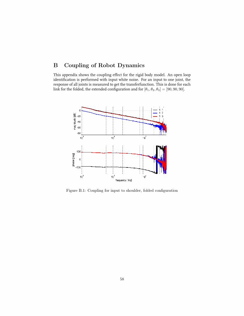
B Coupling of Robot Dynamics
This appendix shows the coupling effect for the rigid body model. An open loopidentification is performed with input white noise. For an input to one joint, theresponse of all joints is measured to get the transferfunction. This is done for eachlink for the folded, the extended configuration and for [θ1, θ2, θ3] = [90, 90, 90].
Figure B.1: Coupling for input to shoulder, folded configuration
58

Figure B.2: Coupling for input to shoulder, [90;90;90] configuration
Figure B.3: Coupling for input to shoulder, extended configuration
59

Figure B.4: Coupling for input to elbow, folded configuration
Figure B.5: Coupling for input to elbow, [90;90;90] configuration
60

Figure B.6: Coupling for input to elbow, extended configuration
Figure B.7: Coupling for input to wrist, folded configuration
61

Figure B.8: Coupling for input to wrist, [90;90;90] configuration
Figure B.9: Coupling for input to wrist, extended configuration
62

C Dynamic Equation as Function of Base Para-meter Set
This part shows the dynamic equations as function of the base parameter set.
M(x) =
I11 I12 I13
I12 I22 I23
I13 I23 I33
(C.1)
with
I11 = a1 + a6 + a5 − 2a2C2 + 2a3C23 − 2a4C3
I22 = a5 − 2a4C3 + a6
I33 = a6
I12 = a5 + a6 − a2C2 + a3C23 − 2a4C3
I13 = a6 + a3C23 − a4C3
I23 = a6 − a4C3
(C.2)
and
h(x) =
h1(x)h2(x)h3(x)
(C.3)
with
h1(x) = a2S2
(x2
5 + 2x4x5
)− a3S23
(x2
5 + x26 + 2x4x5 + 2x4x6 + 2x5x6
)+a4S3
(x2
6 + 2x4x6 + 2x5x6
)h2(x) = −a2S2x
24 + a3S23x
24 + a4S3
(x2
6 + 2x4x6 + 2x5x6
)h3(x) = S23x
24 − a4S3
(x2
4 + x25 + 2x4x5
)where
S2 = sin(x2) C2 = cos(x2)S3 = sin(x3) C3 = cos(x3)S23 = sin(x2 + x3) C23 = cos(x2 + x3)
63

D Relation Digital Input to Torque
This appendix shows the results of the measurement of the digital input of thesystem (DAC) when an external force is applied to the system at R=0.21m.
Figure D.1: Measured DAC for shoulder for 10N, 20N and 30N
Figure D.2: Measured DAC for elbow for 10N and 20N
Figure D.3: Measured DAC for wrist for 6 and 10N
64

E Model Verification
An open loop identification of only the diagonal term of the inertia matrix M foreach link. This is compared to the real spectrum of the system for different config-urations.
Figure E.1: Shoulder clamped open loop model verification
65

Figure E.2: Elbow clamped open loop model verification
Figure E.3: Wrist clamped open loop model verification
66
F Input-Output Linearization and Decoupling viaRestricted State Feedback with DisturbanceRejection
In Tsirikos and Arvanitis (2000) an algebraic approach is treated to find a statefeedback controller which linearizes and decouples the system while disturbancetorques such as friction are rejected by this controller. In this appendix first a sum-mary of the theory is given and next the theory is applied to the dynamic equationsof the SCARA.
F.1 Theory
The robot dynamics can be rewritten in state space form as:
x = E0(x) + E(x)[
uξ
],x(0) = x0,y = z(x) (F.1)
Where E(x) =[
G(x) D(x)]and x =
[x1 x2 x3 x4 x5 x6
]T ∈ Rn,y ∈ Rp and u ∈ Rm, and ξ the disturbance vector due to friction or unknowndisturbance torques. E0 G(x) and D(x) are analytic matrix valued functions of x.
For a nonlinear analytic system of the form of (F.1), the generalized Markovparameters, are defined by:
Mj = LELjE0
z(x) (F.2)
with LjE0
z(x) defined as the jth derivative of z along vector E (Lie-derivative, (au-thor?) (8)). Next apply the nonlinear restricted state feedback control law:
τ = B(x) (a(x) + u) (F.3)
where the external input u ∈ Rp and a(x) and B(x) are analytic matrix valuedfunctions of x.
Then the resulting closed loop system gets the form:
x = E0(x) + E(x)[
uξ
],x(0) = x0,y = z(x) (F.4)
with E0(x) = E0(x) + G(x)B(x)a(x) and E(x) =[
G(x)B(x) D(x)].
The key to solve a decoupling problem lies in modifying the system’s relativedegrees and/or structure at infinity in order to achieve an equality between thosetwo lists of integers.
The system is I/O linearized and decoupled and simultaneously its output isnot affected by the disturbance iff the following relations hold:
67

LEiLk
E0zi(x) = δk,i, ∀i ∈ Jp and k ∈ {0} ∪ J2n−1 (F.5)
LEjLk
E0zi(x) = 0, ∀i, j ∈ Jp, j 6= i and k ∈ {0} ∪ J2n−1 (F.6)
LEjLk
E0zi(x) = 0, ∀i ∈ Jp, j ∈ {p + 1, . . . , p + ξ} and k ∈ {0} ∪ J2n−1 (F.7)
Where δk,i are real numbers not all zero. LEiLk
E0zi(x) =
δ
L
k−1E0
zi
δx E0
!
δx Ej . Equa-tion (F.5) and (F.6) guarantee the linearization and decoupling of the system while(F.7) guarantees the disturbance decoupling.
Rewriting these relations in the next form allows one to formulate the DRLDproblem by restricted state feedback as follows:
• Determine the matrix valued functions a(x) and B(x) of (F.3) which satisfythe following relations:
LEiLγi+k
E0zi(x) = µk,i (F.8)
LEjLγi+k
E0zi(x) = µk,i∀j ∈ Jp+ξ, j 6= i (F.9)
where µk,i , δγi+k,i, with at least one µk,i 6= 0,∀i ∈ Jp and k ∈ {0} ∪ J2n−1
where γi is the relative degree ri of joint iminus one.After several transformations [see (author?) (3)] (F.8) and (F.9) can be written
in the form:
d [δ?(x)] E(x) =[
P0 0]
(F.10)
θi(x)Πi(x) = 0 ∀i ∈ Jp (F.11)
where,
δ?(x) =
LγiE0
zi(x)...
LγpE0
zp(x)
(F.12)
P0 , diag{ρ−10,i
}(F.13)
θi(x) =[
d[
ai
]ρ0,i ρ1,i −ρ2,i · · · (−1)2n−1ρ2n,i
], (F.14)
Πi(x)=[
Πai (x) Πb
i (x)]
(F.15)
In order to make sure the problem defined by (F.10) and (F.11) is solvable for ai(x)and B(x) some conditions need to be fulfilled:
It can be proven that the DRLD problem via the restricted state feedback law issolvable if and only if there exist a set of nonnegative integers
{γ1,s · · · γp,s
}such that the following conditions simultaneously hold:
68
rank {Γ1(x)} − rank {Γ0(x)} = p (F.16)
∆1(x) = 0 (F.17)
with
[Γ0(x) ∆0(x)
]=
M1(1, :)...
Mγ1(1, :)...
M1(p, :)...
Mγp(p, :)
(F.18)
and
[Γ1(x) ∆1(x)
]=
[Γ0(x)∆0(x)
d [δ?(x)][
G(x) D(x)] ]
(F.19)
Then the solution of (F.10) and (F.11) with respect to B(x) gives us
B(x) = W(x)[WT (x)W(x)
]−1
WT (x)RT (x)[R(x)RT (x)
](F.20)
and
a(x) = −P−10
[Lγ1,s+1
E0h1(x) · · · Lγp,s+1
E0hp(x)
]T (F.21)
with R(x) = d [δ?(x)]G(x) and W is a m × σ full column matrix with σ = m −rank {Γ0(x)} which is orthogonal to Γ0
F.2 Applied to SCARA
Consider again the robot dynamics defined by (2.2). In order to obtain the statespace model of the robot manipulator of the form (F.1) some variables are defined:
x =[
θ1 θ2 θ3 θ1 θ2 θ3
]T=
[x1 x2 x3 x4 x5 x6
]T
τ =[
τ1 τ2 τ3
]ζ =
[τv1 τv2 τv3
]T =[
ξ1 ξ2 ξ3
]T
y =[
θ1 θ2 θ3
]T =[
x1 x2 x3
]T
(F.22)Next the inverse of M is calculated:
69

M−1(x) = 1det(M)
I22I33 − I223 I23I13 − I12I33 I12I23 − I22I13
I23I13 − I12I33 I11I33 − I213 I13I12 − I11I23
I12I23 − I22I13 I13I12 − I11I23 I11I22 − I212
=
µ11 µ12 µ13
µ12 µ22 µ23
µ13 µ23 µ33
(F.23)
where Iii are defined by C.2. Then the dynamics can be written in the form F.1with,
E0 =
x4
x5
x6
−M−1(x)h(x)
=
x4
x5
x6
f1(x)f2(x)f3(x)
(F.24)
and
G(x) =[
03×3
M−1(x)
]D(x) =
[03×3
M−1(x)
](F.25)
The Markov parameters are then calculated according to:
M1 = d [h(x)]E(x) = ∂z(x)∂x E(x) = 03×6
M2 = d [LE0z(x)]E(x) =∂(LE0z(x))
∂x E(x) =∂( ∂z(x)
∂x E0)∂x E(x)
=
µ11 µ12 µ13 µ11
µ12 µ22 µ23 µ22
µ13 µ23 µ33 µ33
M3 = d
[L2
E0z(x)
]E(x) =
∂(L2E0
z(x))∂x E(x) =
∂
∂(LE0
z(x))∂x E0(x)
!
∂x E(x)
=
ν11 ν12 ν13 λ11 λ12 λ13
ν21 ν22 ν23 λ21 λ22 λ23
ν31 ν32 ν33 λ31 λ32 λ33
(F.26)
where
νi1 = δfi
δx4µ11 + δfi
δx5µ12 + δfi
δx6µ13
νi2 = δfi
δx4µ12 + δfi
δx5µ22 + δfi
δx6µ23
νi3 = δfi
δx4µ13 + δfi
δx5µ23 + δfi
δx6µ33
λi1 = δfi
δx4µ11
λi2 = δfi
δx5µ22
λi3 = δfi
δx6µ33
(F.27)
The canditates γ1,s, γ2,s, γ3,s are subject to the next constraint:
70

γ1,s ≤ n− 1 = 6− 1 = 5 andn∑
i=1
γi,s ≤ n− p = 6− 3 = 3 (F.28)
, which gives the next canditates γ1,s
γ2,s
γ3,s
=
0 1 0 0 2 0 0 3 0 0 1 1 1 0 1 1 2 0 2 00 0 1 0 0 2 0 0 3 0 1 0 1 1 0 2 1 1 0 20 0 0 1 0 0 2 0 0 3 1 1 0 1 2 0 0 2 1 1
(F.29)
Using any of these canditates will not fulfill all conditions and the DRLD problemis thus not solvable:
• for γi,s = 1 gives ∆0(x) = 0 but ∆1(x) 6= 0 and thus (F.17) is not satisfiedfor any i.
• for γi,s > 1 gives ∆0(x) 6= 0 and thus ∆1(x) 6= 0 and thus (F.17) is notsatisfied for any i.
• for γi,s = 0 gives for (F.16) rank(Γ1(x))− rank(Γ0(x)) = 0 6= p = 3
Since the theory is based on the assumption that p ≤ m, it means that the outputvector y cannot be extended by including the velocities and thus the problem is notsolvable for the SCARA robot if disturbances need to be rejected simultaneously.
Now assume that there is no disturbance vector, i.e. ξ = 0 , and the problemis simplified since matrix D = 0 and condition F.17 does not need to be fulfilled.Then the Markov parameters are derived again:
M1 = 03×3
M2 =
µ11 µ12 µ13
µ12 µ22 µ23
µ13 µ23 µ33
M3 =
ν11 ν12 ν13
ν21 ν22 ν23
ν31 ν32 ν33
(F.30)
and it can be proven that the problem is only solvable for γ1,s = 1, γ2,s = 1, γ3,s = 1and:
W = I3×3 (F.31)
and
R = d [δ?(x)]G(x) =
µ11 µ12 µ13
µ12 µ22 µ23
µ13 µ23 µ33
= M−1 (F.32)
Therefore, the appropiate restricted state feedback is given by:
71

B(x) = IRT[RRT
]−1
P0 = IRT[R2
]−1
P0 = IR
R2P0 = R−1P0 = MP0
(F.33)and
a = −P−10
f1
f2
f3
= P−10 M−1h (F.34)
where the symmetric property of R and P0 = diag{ρ−10,i
}are used. The control
law τ = B(x) (a(x) + u) becomes then:
τ = MP0
(P−1
0 M−1h + u)
= h + MP0u (F.35)
Finally the closed-loop system has the input-ouput description:
y(2)i = ρ−1
0,i wi or H(s) = diag{
s−(γi,s+1)ρ−10,i
}= diag
{1
s2ρ0,i
}(F.36)
and it is shown that the system is decoupled and linearized with the restricted statefeedback. This solution for decoupling and linearization of the SCARA dynamicsresults in a similar controller as the computed torque controller.
72

G Prediction Decoupling Effect
This appendix will show the influence of an error in the model parameters if de-coupling is considered. In the second section the influence of a payload is studied.
G.1 Decoupling for Parameter Error
Since the mathematic model does not match the real system dynamics exactly, theinfluence of parameter errors will be studied when this model is used to decouplethe system. First the decoupling controller is connected to the system model andan openloop identification is performed. In case of no parameter error and nomeasurement quantification, the decoupling is perfect, i.e. the magnitude of thenon-diagonal terms are equal to zero. Inclusion of encoders in the model results inless decoupling but still a minimummagnitude difference of 50 dB is achieved. Inorder to find the worst case of decoupling due to parameter error, the parameters ofthe decoupling controller are changed in positive and negative direction. Since theradius of the links Ri can be measured very accurately and will not change muchduring life time, the number of model parameters is reduced from 12 to 9 in orderto limit the calculation time of the simulations. For each test 29 = 512 simulationshave to be done in order to see which combination of positive and negative variationresults in the worst case. Since the influence of decoupling can be different forother configurations, some tests are performed for different configurations. Firstthe decoupling effect for the first joint in the extended configuration is studied andthe initial parameter error is 20%. Then the error is decreased until decouplingis achieved. In the tables below the magnitude of the spectrum from activatedjoint to all the outputs are shown at 10 Hz. For an error of 7% the worst case ofdecoupling is 8 dB gain difference in amplitude of the spectra between the joint1 and joint 3. For other configurations, better decoupling is achieved. For theelbow and wrist an error of 7 % results in a minimum decoupling effect of 15 dBand 34 dB respectively for the extended configuration. In these simulations, theamplitude of the input signal is further decreased until the system remains in itsinitial configuration. This method cannot be performed on the real system sincethe decoupled system is not necessary stable. Therefore closed loop tests need to beperformed in order to study the decoupling effect. Furthermore it is clear that notonly the model parameters influence the decoupling, but also other effects such asfriction, although small, will deteriorate the decoupling effect.
init = [πππ] init=[000] init=[π2
π2−
π2 ] init=[π
4π4
π4 ]
20% 10% 7% 5% 7% 7% 7%G11 -39 -37 -37 -37 -38 -37 -37G12 -37 -43 -47 -90 -94 -68 -62G13 -34 -41 -45 -62 -49 -45 -87
Table G.1: Amplitude at 10 Hz for input to shoulder, worst case
73

init = [πππ]7%
G21 -88G22 -36G23 -51
init = [πππ]7%
G31 -118G32 -71G33 -37
Table G.2: Amplitude at 10 Hz for input to elbow and wrist, worst case
G.2 Decoupling for Payload
Since the SCARA-robot has to pick up different loads, the worst case decouplingeffect under influence of payload is studied for a system which is decoupled withthe computed torque controller based on the worst case parameter error of 7%. Infigure G.1 a schematic overview of the new parameters in case of payload is given.Then the model parameter m3 changes according to:
m3p = m3 + mp (G.1)
The position of the center of mass changes according to:
L3p =m3L3 + Lpmp
m3p(G.2)
Finally, the inertia can be calculated using Huygens-Steiner’s theorem:
Idisplaced = Icentroid + mR2
I30 + Ip0 = I3p0
I3 + m3L23 + mpL
2p = I3p + m3pL
23p
}→ I3p = I3 + m3L
23 + mpL
2p −m3pL
23p
(G.3)The worst case decoupling is studied by doing simulations for different pay-
loads and different configurations. In table G.3 the worst case is shown for payload0.5 Kg and parameter error 5% in the extended configuration. No decoupling isachieved, but it is still more decoupled than when no decoupling controller is used.For a payload of 0.1 Kg a worst case decoupling effect of 2 dB is achieved. An inputto joint two and three will not influence the shoulder very much which was not thecase when no decoupling controller is used. Finally it can be concluded that underinfluence of a payload no decoupling is achieved. Therefore a method to handlewith this will be proposed in chapter 7.
74

m3 m3p
lp
l3p
l3
mp
k3
Figure G.1: The case of payload
gain [dB] gain [dB] gain [dB]G11 -37 G21 -77 G31 -111G12 -56 G22 -37 G32 -71G13 -37 G23 -39 G33 -40
Table G.3: Amplitude at 10 Hz for input to shoulder, elbow and wrist, worstcase
75
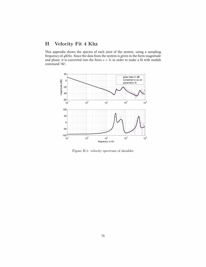
H Velocity Fit 4 Khz
This appendix shows the spectra of each joint of the system, using a samplingfrequency of 4KHz. Since the data from the system is given in the formmagnitudeand phase, it is converted into the form a + bi in order to make a fit with matlabcommand ’tfe’.
10-1
100
101
102
103
-60
-40
-20
0
20velocity frf of scara
magnitude [
dB
]
given data in dB
converted to ax+bi
parametric fit
10-1
100
101
102
103
-100
-50
0
50
100
frequency in Hz
Figure H.1: velocity spectrum of shoulder
76

10-1
100
101
102
103
-40
-30
-20
-10
0
10velocity frf of scara
magnitude [
dB
]
given data in dB
converted to ax+bi
parametric fit
10-1
100
101
102
103
-150
-100
-50
0
50
100
frequency in Hz
Figure H.2: velocity spectrum of elbow
10-1
100
101
102
103
-60
-40
-20
0
20
40velocity frf of scara
magnitude [
dB
]
given data in dB
converted to ax+bi
parametric fit
10-1
100
101
102
103
-200
-150
-100
-50
0
frequency in Hz
Figure H.3: velocity spectrum of wrist
77

I Gains SISO Controllers for Decoupled System
PD PD+lowpass PD+observerωd[Hz] 3.2 5.5 11
ξ[-] 1 1 1ωlp[Hz] 25ωo[Hz] 12.5fco[Hz] 6 12 8
Table I.1: Control gains shoulder
PD PD+lowpass PD+observerωd[Hz] 1.3 2.2 4
ξ[-] 1 1 1ωlp[Hz] 7ωo[Hz] 7fco[Hz] 6 6 5
Table I.2: Control gains Elbow
PD PD+lowpass PD+observerωd[Hz] 4 2.8 12.5
ξ[-] 1 1 1ωlp[Hz] 10ωo[Hz] 13fco[Hz] 7 5.5 8
Table I.3: Control gains Wrist
78

J Decentralized Control
Decentralized control treats each joint separately and can be used when the systemhas large gear ratio’s, i.e. the system is not coupled. In order to make a comparisonwith the decoupling controller, a decentralized control approach is done to controlthe direct drive SCARA. If the gains are high enough it can control the couplingeffect of each link. But the resonances limit the control gains and therefore theperformance will not be very high, since the coupling makes the system unstable.Therefore the PD gains are designed with diet for the different models based on thespectra for several configurations. One of the problems is that the spectrum of theextended configuration differs very much compared to the folded configuration.Therefore one controller must be designed for which the closed loop system isstable for all configurations, since an optimal controller for one configuration canbe unstable for another configuration.
PD Shoulder Elbow Wristgain 0.15 0.1 0.1zero 5 5 5
Table J.1: constants for decentralized control
-60
-40
-20
0
20
40
Magnitu
de (
dB
)
100
101
102
103
-180
-90
0
90
Phase (
deg)
Shoulder CH Bode Diagram
Frequency (Hz)
8EE
8E9
8FF
Figure J.1: Bode diagram Openloop CG for shoulder for different configurations
79

-60
-40
-20
0
20
40
Magnitu
de (
dB
)
100
101
102
103
-180
-90
0
90
180
Pha
se (
de
g)
Elbow CH Bode Diagram
Frequency (Hz)
8EE
8FF
Figure J.2: Bode diagram Openloop CG for elbow for different configurations
-40
-20
0
20
40
Magnitu
de (
dB
)
100
101
102
103
-180
-135
-90
-45
Phase (
deg)
Wrist CH Bode Diagram
Frequency (Hz)
879
8EE
Figure J.3: Bode diagram Openloop CG for wrist for different configurations
80

Since the high frequent dynamics cause the motor to make noise, a low passfilter is added. The cutoff frequency is determined by analyzing the input signal tothe motor. Since this signal contains the low frequent acceleration profile, this datais smoothened and then subtracted from the original data. Next a Fourier transfor-mation is calculated on this signal which results in a cutoff frequency of 120 Hz.See the figure below which contains the output signal for the wrist. For the otherjoints the same cut-off frequency was found. The controller is stable and for thetwo link system, i.e. elbow and wrist, the performance is verified. Since for a twolink SCARA the coupling does not play such a large role, the performance is quitegood. The results are shown in the figures below for a maximal velocity of 6 rad/sand a maximal acceleration of 10 rad/s2. When the third axis is set in closed loopthen the decoupling effect becomes much larger and the system is very likely to be-come unstable. A movement from folded configuration to extended configurationcan be considered as the most critical since at the final stage the decoupling effectand inertia plays a large role. The maximal velocity and accelerations are decreasedto 2 rad/s and 2 rad/s2 respectively. The results are shown below.
vel_max=5 vel_max=2Shoulder - 535Elbow 1948 659Wrist 2051 1617
Table J.2: Maximal dynamic error during motion from folded to extended for atwo-link system and a three-link system
0 200 400 600 800 1000 1200 1400 1600 1800-2500
-2000
-1500
-1000
-500
0
500
1000
1500
2000
2500
time [sample]
positio
nerr
or
Figure J.4: Error signal;original, smoothend and subtracted
81

100
101
102
103
104
0
1
2
3
4
5
6
7
8
frequency [Hz]
magnitude
Figure J.5: Fourier transformation of DAC output
82

K Experimental Results
Comparison Ktau2dac which is calculated, tuned and measured.
Ktau2dac S E Wcalculated 104 256 339
tuned 118 292 356measured 131 283 408
final 131 283 356Max. error K is tuned K is measured
motion Shoulder Elbow Wrist Shoulder Elbow Wrist2 97 -189 -888 85 148 8453 180 575 276 190 630 4094 -327 1174 150 196 760 1785 -528 -1032 -236 479 905 6706 380 -49 448 341 58 4017 -745 -1955 3633 587 1709 4283
Mean 376 829 941 313 702 1131Max. error K final
motion Shoulder Elbow Wrist2 103 171 9173 177 575 3584 199 749 1655 454 825 4986 357 58 3897 544 2355 3725
Mean 305 788 1088
Table K.1: Comparison influence Ktau2dac, parameters S.E
Comparison parameters from Solid Edge to parameters obtained by fitting thespectra:
83

Max. error parameters S.E. Parameters Fitmotion Shoulder Elbow Wrist Shoulder Elbow Wrist
2 103 -171 -917 82 -169 -8833 177 -575 358 166 -520 3444 -199 749 165 -186 733 1585 -454 -825 -498 -422 749 -4816 357 -58 389 346 -61 3897 -544 -2355 3725 520 -2345 3691
Mean 305 788 1088 287 762 991
Table K.2: Comparison influence new parameters from Spectra. Ktau2dac= [131283 356]
The influence of large parameter errors is studied by using the model para-meters of prototype 1 which does not have any clamps build in. Besides that theend-effector has been redesigned and the parameter for this link is calculated forthe case of taking a wafer. In the table below, it is shown that the old parametersare much different than the real system.
Max. error Old parameters SE New parameters SEKtau2dac:118 292 356 Ktau2dac:118 292 356
Motion Shoulder Elbow Wrist Shoulder Elbow Wrist2 164 209 1766 97 189 8883 189 377 294 180 575 2764 376 1077 178 -327 1174 1505 851 1115 317 -528 1032 2366 475 46 457 380 49 4487 856 1918 4824 -745 1955 3633
Mean 485 790 1306 376 829 941
Table K.3: Comparison old vs new parameters, Ktau2dac tuned
parameters m1 I1 L1 m2 I2 L2 m3 I3 L3Old 5.14 0.0589 0.0901 3.87 0.04233 0.11 2.356 0.0516 0.0635New 5.039 0.10176 0.9152 3.82 0.09054 0.112 2.1 0.0229 0.0315
0.0315error 2% 42% 2% 1% 54% 3% 12% 125% 101%
Table K.4: Comparison old parameters vs new parameters
84

Experimental results of final controller This part shows the trajectory erroras function of time for the defined motions.
Shoulder
Elbow
Wrist
All
Extended configuration
Folded Configuration
1 2
4 3
5 6
7 8
shoulder elbow wrist
Figure K.1: Performance motions
85

Figure K.2: Time motion 8
Figure K.3: Time motion 7
86
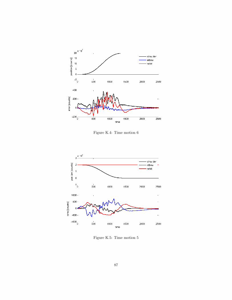
Figure K.4: Time motion 6
Figure K.5: Time motion 5
87
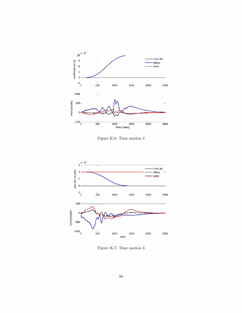
Figure K.6: Time motion 4
Figure K.7: Time motion 3
88

Figure K.8: Time motion 1
89

L Conversion from Velocity to Position
The sweep sine function implemented in the firmware of the system gives a velocityspectrum. Since the outer loop controller is based on the position spectrum thevelocity spectrum has to be converted into position. Since the original file whichwas provided was not correct, some study is done for this case. To convert a velocitymagnitude spectrum to a position spectrum:
Pos(k) =V el(k)Fs
2πf(L.1)
where f is the frequency (in Hertz) of belonging to Pos(k) and Fs the samplefre-quency. The resulting formula when converting the magnitude with units in dB isgiven by:
Pos(k) = V el(k) = 20log10(Fs)− 20log10(2πf) (L.2)
Multiplication with the sample frequency is required since the velocity spectrumis calculated as magnitude per sample. One concern with this technique is thatone can run into problems related to the limited frequency resolution of your spec-tra. In applying the division to each bin, it is assumed that the frequency remainsconstant over the width of the bin. Although this will never be the case with a dis-crete representation of the frequency domain. The accuracy of the conversion canbe improved by increasing the frequency resolution of your spectrum. Finally, thephase of the position spectrum is equal to the velocity spectrum subtracted with 90degrees.
90

M Delay
Because the digital measurement systems may introduce linear delay the samplingdelay Td is determined to simulate the real system more accurately. The linear lagcan be described by: −360·Td ·f , where Td the time-delay in [s] and f the frequencyin [Hz]. The delay is determined for the third joint since this one contains leastresonances and the linear lag is thus best visible, see figure below. As shown thephase drops -60 degrees over 500Hz and thus Td = 60/−360/(f2−f1) = 1/3ms.For the elbow a similar phase lag can be observed.
0 100 200 300 400 500 600 700 800 900 1000-220
-200
-180
-160
-140
-120
-100
-80
-60
-40
-20
Figure M.1: phase of wrist on linear scale
Increase of the sample time causes less delay time since:
Td = Tc + Ts/2
where Td is the delay time, Tc is the computation time and Ts is the sampletime.An increase of the sampletime can increase the performance because this meansless delay time. However, the encoder resolution will limit the increase of the sam-plefrequency.
For example: Samplefrequency Fs is equal to 1 kHz. The measurement systemresolution is equal to 2π/4e6 rad/enc. If the servo speed is set to 10 rad/s, then thisgives 6360 encodercounts/sampletime which is high enough to be accurate. Thismeans that the samplefrequency could be increased. Since the desired bandwidthis set to 10 Hz a samplefrequency of 1000 Hz is considered to be high enough.
91

N PD Control of Vertical Axis
To compare the performance of the adaptive control, a PD controller is designed.First a openloop sweptsine identification is done, with gravity compensation en-abled. The velocity spectrum of the vertical axis is obtained at different heights andconverted to position spectrum, see figure below. In order to compare the modelof the simulations with the real system, the magnitude of the spectrum at 10 Hzis compared. Since the spectrum is from DAC output to encoders it is converted.The relation from DAC to Force is equal to 1 and conversion from encoders to me-ters is given by 20*log10(0.000444e-3)=-127dB. As shown in figure below, the gainat 10Hz is -13dB, so -13-127= -140dB. Since this is comparable to -150 dB it is as-sumed that the model is correct. During this identification, gravity compensationwas enabled otherwise the motion would be not the same for a motion upwardsand a motion downwards. When designing a controller in frequency domain, oneshould take into account this gravity factor which is equal to F=m*g=200N. Thespectrum therefore has to be multiplied with a factor 200=46dB
As expected, the spectrum doesn’t change much for different heights. A fit ofone of the spectra is made. Since the spectra are not correct for low and very highfrequencies, a fit is made while excluding the low and high frequencies, i.e below40Hz and above 800Hz. The next control parameters are obtained:
PD gain 1zero 60
lowpass filter cutoff freq [Hz] 400damping 0.7
Table N.1: Control parameters PD
92

Figure N.1: Velocity FRF of vertical axis (blue) and fit (black), 4 kHz
Figure N.2: Open loop spectrum CH
93