Embed Size (px)
Citation preview
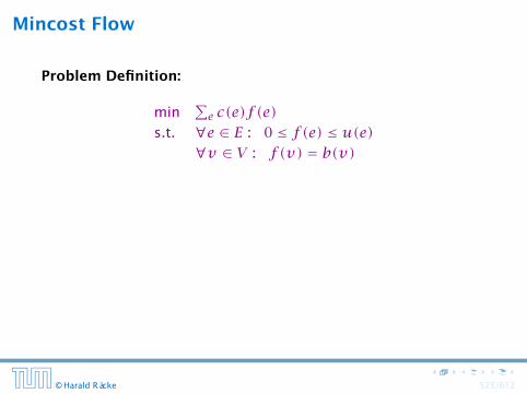
Mincost Flow
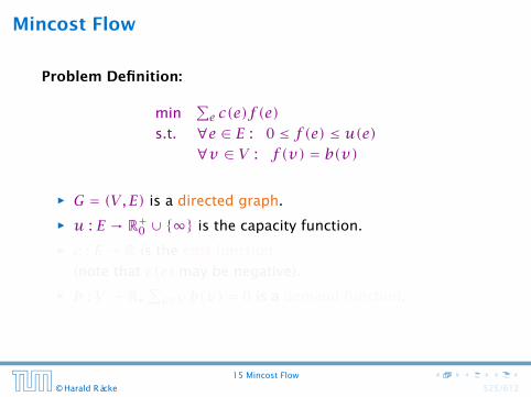
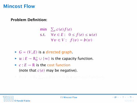
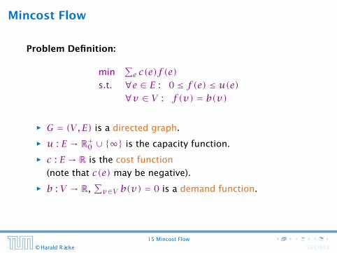
Problem Definition:
min∑e c(e)f (e)
s.t. ∀e ∈ E : 0 ≤ f(e) ≤ u(e)∀v ∈ V : f(v) = b(v)
ñ G = (V , E) is a directed graph.
ñ u : E → R+0 ∪ {∞} is the capacity function.
ñ c : E → R is the cost function
(note that c(e) may be negative).
ñ b : V → R,∑v∈V b(v) = 0 is a demand function.
© Harald Räcke 525/612
Mincost Flow
Problem Definition:
min∑e c(e)f (e)
s.t. ∀e ∈ E : 0 ≤ f(e) ≤ u(e)∀v ∈ V : f(v) = b(v)
ñ G = (V , E) is a directed graph.
ñ u : E → R+0 ∪ {∞} is the capacity function.
ñ c : E → R is the cost function
(note that c(e) may be negative).
ñ b : V → R,∑v∈V b(v) = 0 is a demand function.
15 Mincost Flow
© Harald Räcke 525/612

Solve Maxflow Using Mincost Flow
s
2
3
4
5
6
7
t
10
5
15
4
9
15
4
8
30
6
15
15
10
10
10
ñ Given a flow network for a standard maxflow problem.ñ Set b(v) = 0 for every node. Keep the capacity function u
for all edges. Set the cost c(e) for every edge to 0.ñ Add an edge from t to s with infinite capacity and cost −1.ñ Then, val(f∗) = − cost(fmin), where f∗ is a maxflow, and
fmin is a mincost-flow.
15 Mincost Flow
© Harald Räcke 526/612

Solve Maxflow Using Mincost Flow
s
2
3
4
5
6
7
t
10
5
15
4
9
15
4
8
30
6
15
15
10
10
10
ñ Given a flow network for a standard maxflow problem.
ñ Set b(v) = 0 for every node. Keep the capacity function ufor all edges. Set the cost c(e) for every edge to 0.
ñ Add an edge from t to s with infinite capacity and cost −1.ñ Then, val(f∗) = − cost(fmin), where f∗ is a maxflow, and
fmin is a mincost-flow.
15 Mincost Flow
© Harald Räcke 526/612

Solve Maxflow Using Mincost Flow
s
2
3
4
5
6
7
t
10
5
15
4
9
15
4
8
30
6
15
15
10
10
10
ñ Given a flow network for a standard maxflow problem.ñ Set b(v) = 0 for every node. Keep the capacity function u
for all edges. Set the cost c(e) for every edge to 0.
ñ Add an edge from t to s with infinite capacity and cost −1.ñ Then, val(f∗) = − cost(fmin), where f∗ is a maxflow, and
fmin is a mincost-flow.
15 Mincost Flow
© Harald Räcke 526/612

Solve Maxflow Using Mincost Flow
s
2
3
4
5
6
7
t
10
5
15
4
9
15
4
8
30
6
15
15
10
10
10
ñ Given a flow network for a standard maxflow problem.ñ Set b(v) = 0 for every node. Keep the capacity function u
for all edges. Set the cost c(e) for every edge to 0.ñ Add an edge from t to s with infinite capacity and cost −1.
ñ Then, val(f∗) = − cost(fmin), where f∗ is a maxflow, and
fmin is a mincost-flow.
15 Mincost Flow
© Harald Räcke 526/612

Solve Maxflow Using Mincost Flow
s
2
3
4
5
6
7
t
10
5
15
4
9
15
4
8
30
6
15
15
10
10
10
ñ Given a flow network for a standard maxflow problem.ñ Set b(v) = 0 for every node. Keep the capacity function u
for all edges. Set the cost c(e) for every edge to 0.ñ Add an edge from t to s with infinite capacity and cost −1.ñ Then, val(f∗) = − cost(fmin), where f∗ is a maxflow, and
fmin is a mincost-flow.
15 Mincost Flow
© Harald Räcke 526/612

Solve Maxflow Using Mincost Flow
Solve decision version of maxflow:
ñ Given a flow network for a standard maxflow problem, and
a value k.
ñ Set b(v) = 0 for every node apart from s or t. Set b(s) = −kand b(t) = k.
ñ Set edge-costs to zero, and keep the capacities.
ñ There exists a maxflow of value k if and only if the
mincost-flow problem is feasible.
15 Mincost Flow
© Harald Räcke 527/612
Generalization
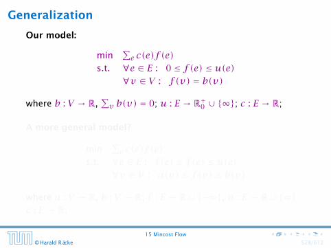
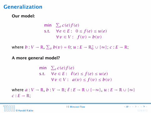
Our model:
min∑e c(e)f (e)
s.t. ∀e ∈ E : 0 ≤ f(e) ≤ u(e)∀v ∈ V : f(v) = b(v)
where b : V → R,∑v b(v) = 0; u : E → R+0 ∪ {∞}; c : E → R;
A more general model?
min∑e c(e)f (e)
s.t. ∀e ∈ E : `(e) ≤ f(e) ≤ u(e)∀v ∈ V : a(v) ≤ f(v) ≤ b(v)
where a : V → R, b : V → R; ` : E → R∪ {−∞}, u : E → R∪ {∞}c : E → R;
15 Mincost Flow
© Harald Räcke 528/612
Generalization
Our model:
min∑e c(e)f (e)
s.t. ∀e ∈ E : 0 ≤ f(e) ≤ u(e)∀v ∈ V : f(v) = b(v)
where b : V → R,∑v b(v) = 0; u : E → R+0 ∪ {∞}; c : E → R;
A more general model?
min∑e c(e)f (e)
s.t. ∀e ∈ E : `(e) ≤ f(e) ≤ u(e)∀v ∈ V : a(v) ≤ f(v) ≤ b(v)
where a : V → R, b : V → R; ` : E → R∪ {−∞}, u : E → R∪ {∞}c : E → R;
15 Mincost Flow
© Harald Räcke 528/612
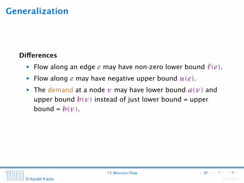
Generalization
Differences
ñ Flow along an edge e may have non-zero lower bound `(e).ñ Flow along e may have negative upper bound u(e).ñ The demand at a node v may have lower bound a(v) and
upper bound b(v) instead of just lower bound = upper
bound = b(v).
15 Mincost Flow
© Harald Räcke 529/612

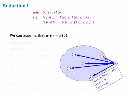
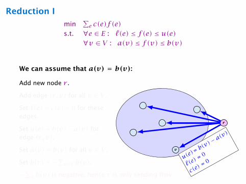
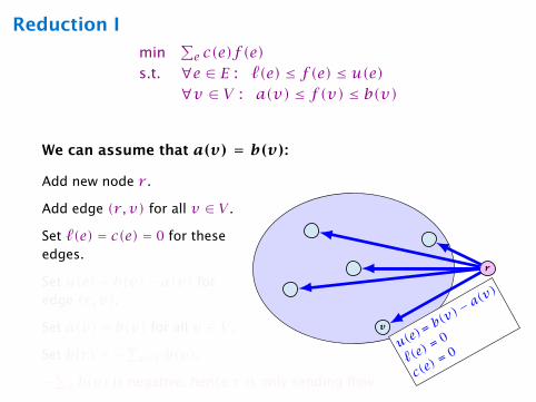
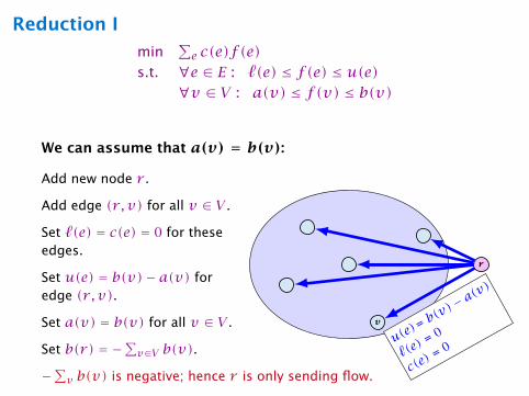
Reduction I
min∑e c(e)f (e)
s.t. ∀e ∈ E : `(e) ≤ f(e) ≤ u(e)∀v ∈ V : a(v) ≤ f(v) ≤ b(v)
We can assume that a(v) = b(v):
Add new node r .
Add edge (r , v) for all v ∈ V .
Set `(e) = c(e) = 0 for theseedges.
Set u(e) = b(v)− a(v) foredge (r , v).
Set a(v) = b(v) for all v ∈ V .
Set b(r) = −∑v∈V b(v).−∑v b(v) is negative; hence r is only sending flow.
v
r
u(e)=b(v
)− a(v)
`(e) = 0
c(e) = 0
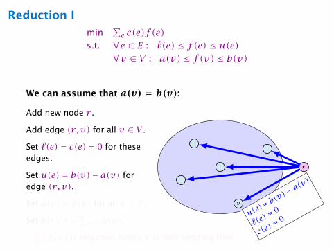
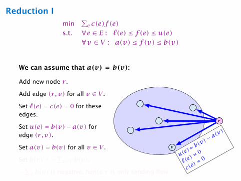
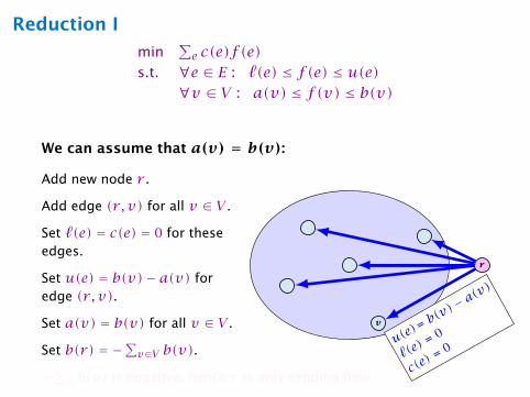
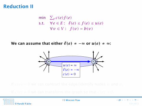
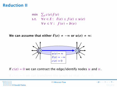
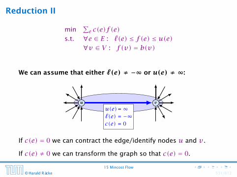
Reduction II
min∑e c(e)f (e)
s.t. ∀e ∈ E : `(e) ≤ f(e) ≤ u(e)∀v ∈ V : f(v) = b(v)
We can assume that either `(e) ≠ −∞ or u(e) ≠ ∞:
u v
u(e)= ∞`(e) = −∞c(e) = 0
If c(e) = 0 we can contract the edge/identify nodes u and v.
If c(e) ≠ 0 we can transform the graph so that c(e) = 0.
15 Mincost Flow
© Harald Räcke 531/612
Reduction II
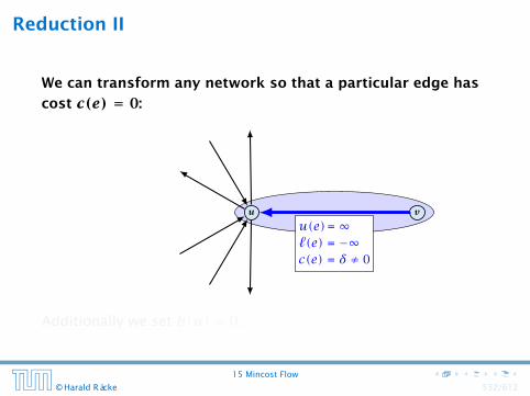
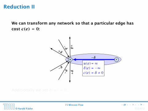
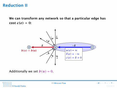
We can transform any network so that a particular edge has
cost c(e) = 0:
x
b(x) = b(u)u v
+δ−δ
+δ
−δ−δ +δ
u(e)= ∞`(e) = −∞c(e) = δ ≠ 0
−δ
Additionally we set b(u) = 0.
15 Mincost Flow
© Harald Räcke 532/612
Reduction II
We can transform any network so that a particular edge has
cost c(e) = 0:
x
b(x) = b(u)u v
+δ−δ
+δ
−δ−δ +δ
u(e)= ∞`(e) = −∞c(e) = δ ≠ 0
−δ
Additionally we set b(u) = 0.
15 Mincost Flow
© Harald Räcke 532/612
Reduction II
We can transform any network so that a particular edge has
cost c(e) = 0:
x
b(x) = b(u)u v
+δ−δ
+δ
δ
−δ−δ +δ
u(e)= ∞`(e) = −∞c(e) = δ ≠ 0
−δ
Additionally we set b(u) = 0.
15 Mincost Flow
© Harald Räcke 532/612
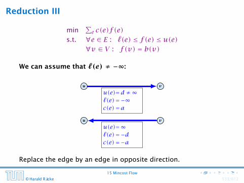
Reduction III
min∑e c(e)f (e)
s.t. ∀e ∈ E : `(e) ≤ f(e) ≤ u(e)∀v ∈ V : f(v) = b(v)
We can assume that `(e) ≠ −∞:
u v
u v
u(e)=d ≠∞`(e)=−∞c(e)=a
u(e)=∞`(e)=−dc(e)=−a
Replace the edge by an edge in opposite direction.
15 Mincost Flow
© Harald Räcke 533/612
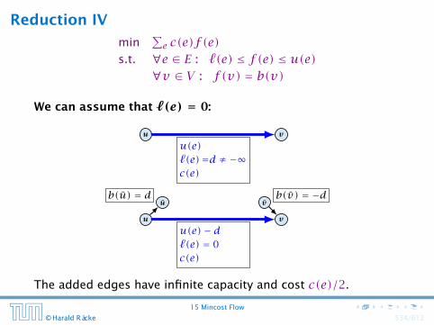
Reduction IV
min∑e c(e)f (e)
s.t. ∀e ∈ E : `(e) ≤ f(e) ≤ u(e)∀v ∈ V : f(v) = b(v)
We can assume that `(e) = 0:
u v
u v
u(e)`(e)=d ≠ −∞c(e)
u(e)− d`(e) = 0c(e)
u vb(u) = d b(v) = −d
The added edges have infinite capacity and cost c(e)/2.
15 Mincost Flow
© Harald Räcke 534/612

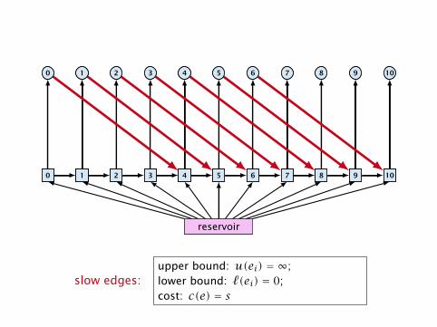
Applications
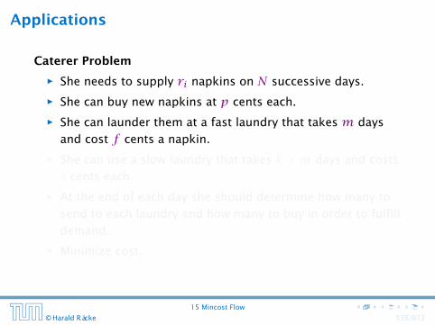
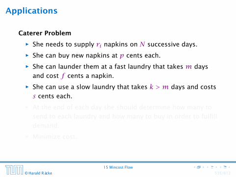
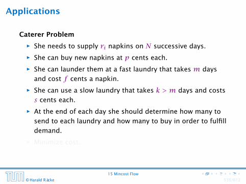
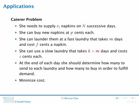
Caterer Problem
ñ She needs to supply ri napkins on N successive days.
ñ She can buy new napkins at p cents each.
ñ She can launder them at a fast laundry that takes m days
and cost f cents a napkin.
ñ She can use a slow laundry that takes k > m days and costs
s cents each.
ñ At the end of each day she should determine how many to
send to each laundry and how many to buy in order to fulfill
demand.
ñ Minimize cost.
15 Mincost Flow
© Harald Räcke 535/612

Applications
Caterer Problem
ñ She needs to supply ri napkins on N successive days.
ñ She can buy new napkins at p cents each.
ñ She can launder them at a fast laundry that takes m days
and cost f cents a napkin.
ñ She can use a slow laundry that takes k > m days and costs
s cents each.
ñ At the end of each day she should determine how many to
send to each laundry and how many to buy in order to fulfill
demand.
ñ Minimize cost.
15 Mincost Flow
© Harald Räcke 535/612

reservoir
trash
reservoir
trash
reservoir
trash
10
10
10
10
9
9
9
9
8
8
8
8
7
7
7
7
6
6
6
6
5
5
5
5
4
4
4
4
3
3
3
3
2
2
2
2
1
1
1
1
0
0
0
0
reservoir
trash
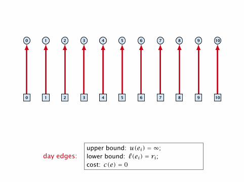
day edges:upper bound: u(ei) = ∞;lower bound: `(ei) = ri;cost: c(e) = 0
reservoir
trash
10
10
10
10
9
9
9
9
8
8
8
8
7
7
7
7
6
6
6
6
5
5
5
5
4
4
4
4
3
3
3
3
2
2
2
2
1
1
1
1
0
0
0
0
reservoir
trash
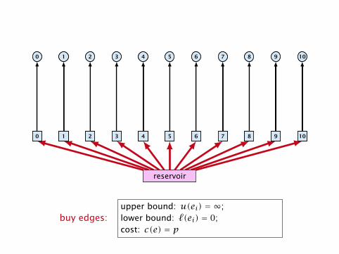
buy edges:upper bound: u(ei) = ∞;lower bound: `(ei) = 0;cost: c(e) = p
reservoir
trash
10
10
10
10
9
9
9
9
8
8
8
8
7
7
7
7
6
6
6
6
5
5
5
5
4
4
4
4
3
3
3
3
2
2
2
2
1
1
1
1
0
0
0
0
reservoir
trash
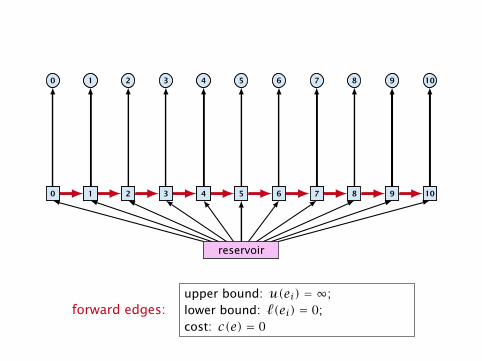
forward edges:upper bound: u(ei) = ∞;lower bound: `(ei) = 0;cost: c(e) = 0
reservoir
trash
10
10
10
10
9
9
9
9
8
8
8
8
7
7
7
7
6
6
6
6
5
5
5
5
4
4
4
4
3
3
3
3
2
2
2
2
1
1
1
1
0
0
0
0
reservoir
trash
slow edges:upper bound: u(ei) = ∞;lower bound: `(ei) = 0;cost: c(e) = s
reservoir
trash
10
10
10
10
9
9
9
9
8
8
8
8
7
7
7
7
6
6
6
6
5
5
5
5
4
4
4
4
3
3
3
3
2
2
2
2
1
1
1
1
0
0
0
0
reservoir
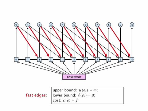
trash
fast edges:upper bound: u(ei) = ∞;lower bound: `(ei) = 0;cost: c(e) = f
reservoir
trash
10
10
10
10
9
9
9
9
8
8
8
8
7
7
7
7
6
6
6
6
5
5
5
5
4
4
4
4
3
3
3
3
2
2
2
2
1
1
1
1
0
0
0
0
reservoir
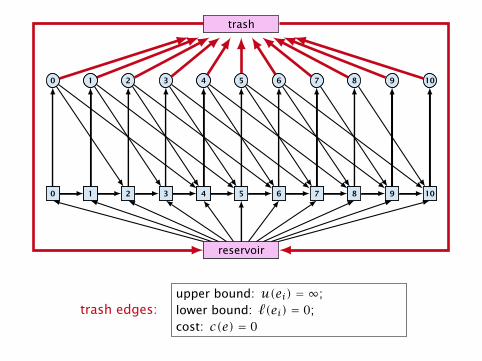
trash
trash edges:upper bound: u(ei) = ∞;lower bound: `(ei) = 0;cost: c(e) = 0
reservoir
trash
10
10
10
10
9
9
9
9
8
8
8
8
7
7
7
7
6
6
6
6
5
5
5
5
4
4
4
4
3
3
3
3
2
2
2
2
1
1
1
1
0
0
0
0
reservoir
trash
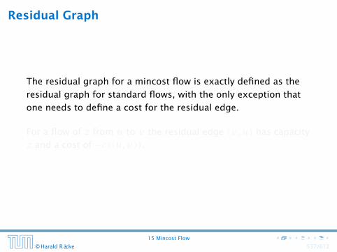
Residual Graph
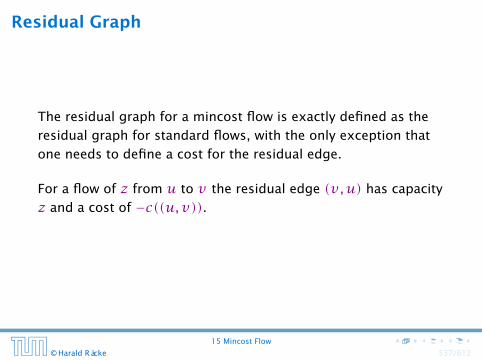
The residual graph for a mincost flow is exactly defined as the
residual graph for standard flows, with the only exception that
one needs to define a cost for the residual edge.
For a flow of z from u to v the residual edge (v,u) has capacity
z and a cost of −c((u,v)).
15 Mincost Flow
© Harald Räcke 537/612
Residual Graph
The residual graph for a mincost flow is exactly defined as the
residual graph for standard flows, with the only exception that
one needs to define a cost for the residual edge.
For a flow of z from u to v the residual edge (v,u) has capacity
z and a cost of −c((u,v)).
15 Mincost Flow
© Harald Räcke 537/612

15 Mincost Flow
A circulation in a graph G = (V , E) is a function f : E → R+ that
has an excess flow f(v) = 0 for every node v ∈ V .
A circulation is feasible if it fulfills capacity constraints, i.e.,
f(e) ≤ u(e) for every edge of G.
15 Mincost Flow
© Harald Räcke 538/612

15 Mincost Flow
A circulation in a graph G = (V , E) is a function f : E → R+ that
has an excess flow f(v) = 0 for every node v ∈ V .
A circulation is feasible if it fulfills capacity constraints, i.e.,
f(e) ≤ u(e) for every edge of G.
15 Mincost Flow
© Harald Räcke 538/612
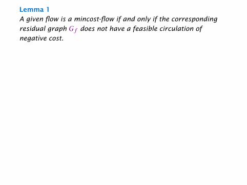
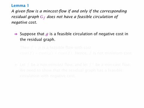
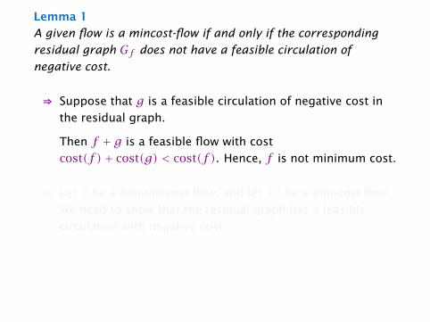
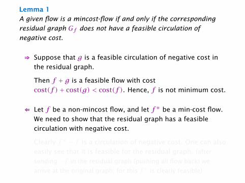
Lemma 1
A given flow is a mincost-flow if and only if the corresponding
residual graph Gf does not have a feasible circulation of
negative cost.
⇒ Suppose that g is a feasible circulation of negative cost in
the residual graph.
Then f + g is a feasible flow with cost
cost(f )+ cost(g) < cost(f ). Hence, f is not minimum cost.
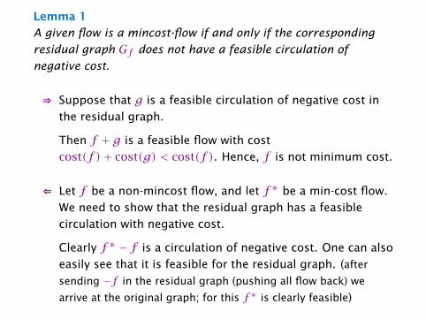
⇐ Let f be a non-mincost flow, and let f∗ be a min-cost flow.
We need to show that the residual graph has a feasible
circulation with negative cost.
Clearly f∗ − f is a circulation of negative cost. One can also
easily see that it is feasible for the residual graph. (after
sending −f in the residual graph (pushing all flow back) we
arrive at the original graph; for this f∗ is clearly feasible)
Lemma 1
A given flow is a mincost-flow if and only if the corresponding
residual graph Gf does not have a feasible circulation of
negative cost.
⇒ Suppose that g is a feasible circulation of negative cost in
the residual graph.
Then f + g is a feasible flow with cost
cost(f )+ cost(g) < cost(f ). Hence, f is not minimum cost.
⇐ Let f be a non-mincost flow, and let f∗ be a min-cost flow.
We need to show that the residual graph has a feasible
circulation with negative cost.
Clearly f∗ − f is a circulation of negative cost. One can also
easily see that it is feasible for the residual graph. (after
sending −f in the residual graph (pushing all flow back) we
arrive at the original graph; for this f∗ is clearly feasible)
15 Mincost Flow
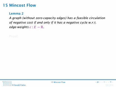
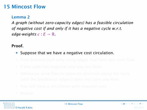
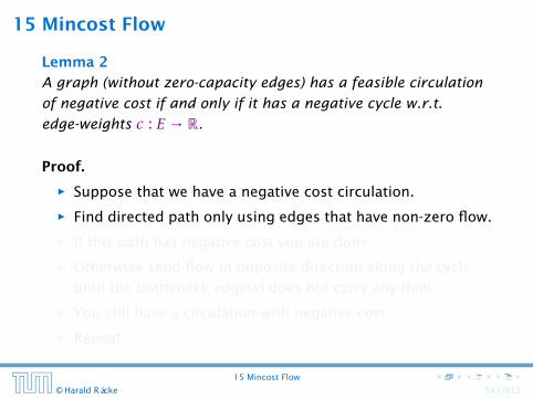
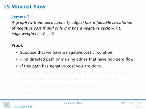
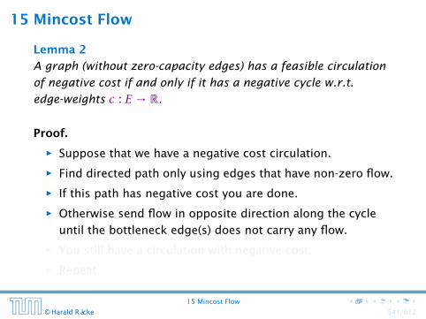
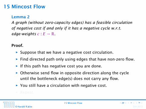
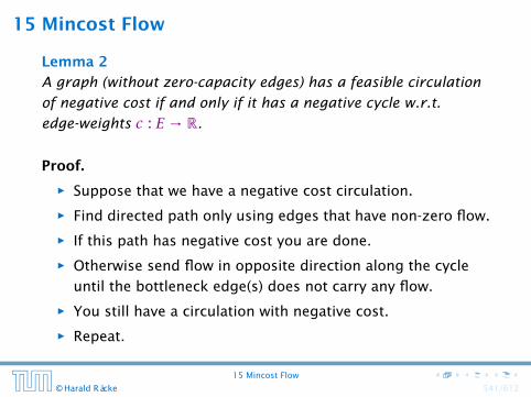
Lemma 2
A graph (without zero-capacity edges) has a feasible circulation
of negative cost if and only if it has a negative cycle w.r.t.
edge-weights c : E → R.
Proof.
ñ Suppose that we have a negative cost circulation.
ñ Find directed path only using edges that have non-zero flow.
ñ If this path has negative cost you are done.
ñ Otherwise send flow in opposite direction along the cycle
until the bottleneck edge(s) does not carry any flow.
ñ You still have a circulation with negative cost.
ñ Repeat.
15 Mincost Flow
© Harald Räcke 541/612
15 Mincost Flow
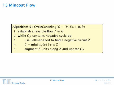
Algorithm 51 CycleCanceling(G = (V , E), c,u, b)1: establish a feasible flow f in G2: while Gf contains negative cycle do
3: use Bellman-Ford to find a negative circuit Z4: δ←min{uf (e) | e ∈ Z}5: augment δ units along Z and update Gf
15 Mincost Flow
© Harald Räcke 542/612
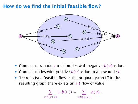
How do we find the initial feasible flow?
x1
x2
x3
x4
x5
x6
x7
ts −b(x1)−b(x1)−b(x2)−b(x2)
−b(x3)−b(x3)
b(x4)b(x4)
b(x5)b(x5)
b(x6)b(x6)
b(x7)b(x7)
ñ Connect new node s to all nodes with negative b(v)-value.
ñ Connect nodes with positive b(v)-value to a new node t.ñ There exist a feasible flow in the original graph iff in the
resulting graph there exists an s-t flow of value∑v :b(v)<0
(−b(v)) =∑
v :b(v)>0
b(v) .
15 Mincost Flow
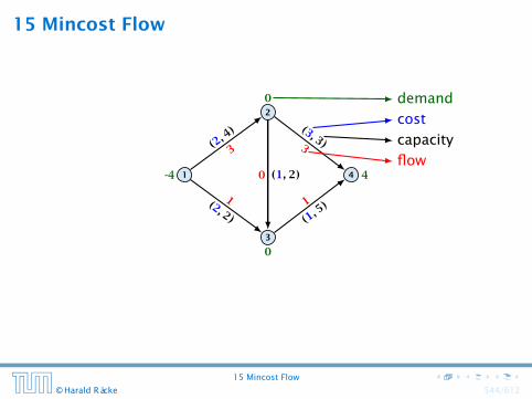
1
2
3
4
(2, 4)
3
(1, 2)0
1(2, 2)1
(1, 5)
(3, 3)3
0
-4 4
0
demand
cost
capacity
flow
15 Mincost Flow
© Harald Räcke 544/612
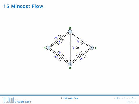
15 Mincost Flow
1
2
3
4
(2, 1)
(-2, 3) (-3, 3)
(3, 2)
(1, 2)(-1, 2)(2, 1)(-2, 1)
(1, 4)
(-1, 1)
0
-4 4
0
15 Mincost Flow
© Harald Räcke 545/612
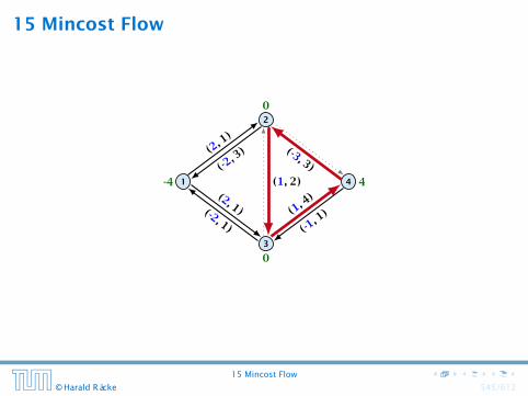
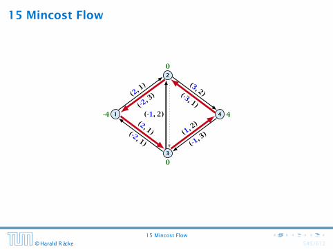
15 Mincost Flow
1
2
3
4
(2, 1)
(-2, 3) (-3, 3)
(3, 2)
(1, 2)(-1, 2)(2, 1)(-2, 1)
(1, 4)
(-1, 1)
0
-4 4
0
15 Mincost Flow
© Harald Räcke 545/612
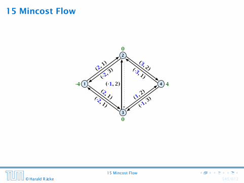
15 Mincost Flow
1
2
3
4
(2, 1)
(-2, 3) (-3, 1)
(3, 2)
(1, 2)(-1, 2)(2, 1)(-2, 1)
(1, 2)
(-1, 3)
0
-4 4
0
15 Mincost Flow
© Harald Räcke 545/612
15 Mincost Flow
1
2
3
4
(2, 1)
(-2, 3) (-3, 1)
(3, 2)
(1, 2)(-1, 2)(2, 1)(-2, 1)
(1, 2)
(-1, 3)
0
-4 4
0
15 Mincost Flow
© Harald Räcke 545/612
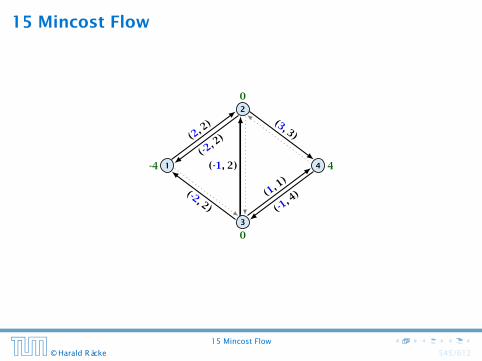
15 Mincost Flow
1
2
3
4
(2, 2)
(-2, 2) (-3, 1)
(3, 3)
(1, 2)(-1, 2)(2, 1)(-2, 2)
(1, 1)
(-1, 4)
0
-4 4
0
15 Mincost Flow
© Harald Räcke 545/612
15 Mincost Flow
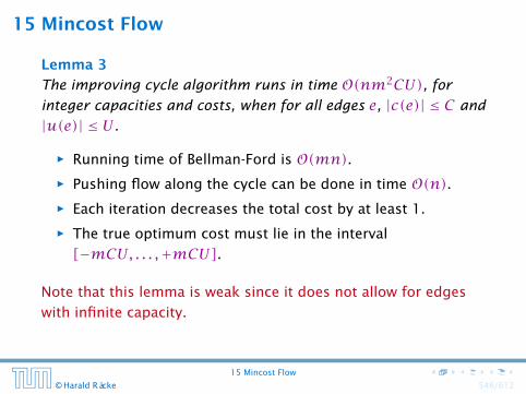
Lemma 3
The improving cycle algorithm runs in time O(nm2CU), for
integer capacities and costs, when for all edges e, |c(e)| ≤ C and
|u(e)| ≤ U .
ñ Running time of Bellman-Ford is O(mn).ñ Pushing flow along the cycle can be done in time O(n).ñ Each iteration decreases the total cost by at least 1.
ñ The true optimum cost must lie in the interval
[−mCU, . . . ,+mCU].
Note that this lemma is weak since it does not allow for edges
with infinite capacity.
15 Mincost Flow
© Harald Räcke 546/612

15 Mincost Flow
A general mincost flow problem is of the following form:
min∑e c(e)f (e)
s.t. ∀e ∈ E : `(e) ≤ f(e) ≤ u(e)∀v ∈ V : a(v) ≤ f(v) ≤ b(v)
where a : V → R, b : V → R; ` : E → R∪ {−∞}, u : E → R∪ {∞}c : E → R;
Lemma 4 (without proof)
A general mincost flow problem can be solved in polynomial
time.
15 Mincost Flow
© Harald Räcke 547/612


![Learning Bayesian Networks in R · 2013-07-10 · Bayesian Networks Essentials Bayesian Networks Bayesian networks [21, 27] are de ned by: anetwork structure, adirected acyclic graph](https://img.pdfslide.net/doc/110x75/5f3267ce969e2b02050fd06c/learning-bayesian-networks-in-r-2013-07-10-bayesian-networks-essentials-bayesian.jpg)


![Modelling Survey Data with Bayesian Networks · Bayesian Networks Bayesian networks (BNs) [6, 13] are de ned by: anetwork structure, adirected acyclic graph G= (V;A), in which each](https://img.pdfslide.net/doc/110x75/5f7ae6fe29c2f22666694c4e/modelling-survey-data-with-bayesian-networks-bayesian-networks-bayesian-networks.jpg)