Minicomputer Capabilities

.5b NUREG/CR-2162 PNL-3773

Related to Meteorological Aspects of Emergency Response

Prepared by J. V. Ramsdell, G. F. Athey, M. Y. Ballinger

Pacific Northwest laboratory Operated by Battelle Memorial Institute

Prepared for U.S. Nuclear Regulatory Commission

NOTICE

This report was prepared as an account of work sponsored by an agency of the United States Government. Neither the United States Government nor any agency thereof, or any of their employees, makes any warranty, expressed or implied, or assumes any legal liability or responsibility for any third party's use, or the results of such use, of any information, apparatus product or process disclosed in this report, or represents that its use by such third party would not infringe privately owned rights.

Available from

GPO Sales Program Division of Technical Information and Docu~ent Control

U. S. Nuclear Regulatory Commission Washington, D. C. 20555

Printed copy price: $5.00

and

National Technical Information Service Springfield, Virginia 22161

3 3679 00059 8781

Minicomputer Capabilities

NUREG/CR-2162 PNL-3773 RB, R6

Related to Meteorological Aspects of Emergency Response

Manuscript ComPleted: December 1981 Date Published: February 1982

Prepared by J. V. Ramsdell, G. F. Athey, M. Y. Ballinger

Pacific Northwest Laboratory Richland, WA 99352

Prepared for Division of Health, Siting and Waste Management Offke of Nuclear Regulatory Research U.S. Nuclear Regulatory Commission Washington, D.C. 20555 NRC FIN 82081

Availability of Reference Materials Cited in NRC Publications

Most documents cited in NRC publications will be available from one of the following sources:

1. The NRC Public Document Room, 1717 H Street, N.W. Washington, DC 20555

2. The NRC/GPO Sales Program, U.S. Nuclear Regulatory Commission, Washington, DC 20555

3. The National Technical Information Service, Springfield, VA 22161

Although the listing that follows represents the majority of documents cited in NRC publications, it is not intended to be exhaustive.

Referenced documents available for inspection and copying for a fee from the NRC Public Docu­ment· Room include NRC correspondence and internal NRC memoranda; NRC Office of Inspection and Enforcement bulletins, circulars, information notices, inspection .. and investigation notices; Licensee Event Reports; vendor reports and correspondence; Commission papers; and applicant and licensee documents and correspondence.

The following documents in the NUREG series are available for purchase from the NRC/GPO Sales Program: formal NRC staff and contractor reports, NRC-sponsored conference proceedings, and NRC booklets and brochures. Also available are Regulatory Guides, NRC regulations in the Code of Federal Regulations, and Nuclear Regulatory Commission Issuances.

Documents available from the National Technical Information Service include NUREG series reports and technical reports prepared by other federal agencies and reports prepared by the Atomic Energy Commission, forerunner agency to the Nuclear Regulatory Commission.

Documents available from public and special technical libraries include all open literature items, such as books, journal and periodical articles, and transactions. Federal Register notices, federal and state legislation, and congressional reports can usually be obtained from these libraries.

Documents such as theses, dissertations, foreign reports and translations, and non-NRC conference proceedings are available for purchase from the organization sponsoring the publication cited.

Single copies of NRC draft reports are available free upon written request to the Division of Tech· nical Information and Document Control, U.S. Nuclear Regulatory Commission, Washington, DC 20555.

Copies of industry codes and standards used in a substantive manner in the NRC regulatory process are maintained at the NRC Library, 7920 Norfolk Avenue, Bethesda, Maryland, and are available there for reference use by the public. Codes and standards are usually copyrighted and may be purchased from the originating organization or, if they are American National Standards, from the American National Standards Institute, 1430 Broadway, New York, NY 10018.

ABSTRACl

The purpose of this report is to provide the NRC staff involved in review­ing licensee emergency response plans with background information on the capa­bilities of minicomputer systems that are related to the collection and dissemination of meteorological infonmation. The treatment of meteorological information by organizations with existing emergency response capabilities is described, and the capabilities, reliability and availability of minicomputers and minicomputer systems are discussed.

iii

ACKNOWLEDGMENTS

Many people contributed to this work by taking the time to talk with us. We wish to thank them and the organizations that they represent for making the time and information available.

We also wish to thank Ron Hadlock and Jim Droppo who, because of their proximity and expertise, were consulted frequently, and Dee Hammer who gave secretarial assistance.

Finally, we wish to thank Dr. Robert F. Abbey, Jr., our NRC technical monitor, for his guidance and assistance.

v

SUr+IARY

The Nuclear Regulatory Commission requires licensees to develop and main­tain an emergency response capability that includes the assess~ent of the poten­tial consequences of accidental releases of material to the atmosphere. The purpose of this report is to provide the NRC staff involved in reviewing licen­see response plans with background information on the capabilities of minicom­puter systems that are related to the collection and dissemination of meteorological information. The names of organizations and specific computer products are used throughout the report to provide concrete examples for dis­cussion. This use does not constitute an endorsement of the organizations or products. Similarly, the failure to name other organizations and products does not constitute a judgment of their values.

To assemble this background information. the staff of the Pacific Northwest Laboratory completed tasks in two areas: identification and evaluation of the methods of treating meteorological information by organizations with existing emergency response capabilities and identification and evaluation of the capability, reliability and availability of existing minicomputers and minicom­puter system components. Information in the first area was obtained by review­ing literature. telephone conservations with knowledgeable individuals, and visits to several nuclear facilities and meteorological consulting organizations for discussions and demonstrations of their emergency response capabilities. In the second area, information was obtained by reviewing recent computer litera­ture and texts on computer system design and evaluation and by visiting compu­ter system manufacturers and dealers. Guidance in estimating computer system requirements was obtained from NUREG-0654, NUREG-0696, and Regulatory Guide 1.23.

State-of-the-art emergency response capabilities use micro- and minicom­puter technology. The organizations visited used micro- and minicomputers for meteorological data acquisition, storage, analysis and dissemination. Atmos­pheric transport and diffusion models incorporating spatial and temporal meteoro­logical variability are being run on minicomputers and are producing timely results. Representative state-of-the-art emergency response capabilities are described in summary form in the tables on pages 14 and 15. The capabilities described are state-of-the-art with respect to the treatment of meteorological information for emergency response applications, but the computer systems used are not necessarily state-of-the-art. In particular, the use of color graphics displays is not common.

Minicomputer capabilities are extensive. The arithmetic precision of minicomputers is similar to that found in many mainframe computers. Minicom­puters can include large memories. and they can drive a wide variety of peri­pheral devices. In many respects it is difficult to distinguish between the capabilities of minicomputers and mainframe computers. The computational speed of typical minicomputers tends to be lower than those of mainframe computers. However, special arithmetic processors are available for minicomputers that have speeds that exceed the speeds of typical mainframes. The array of peri­pheral devices available for minicomputers includes: magnetic tape and disk

vii

storage units, alphanumeric and graphics terminals, card and paper tape readers and punches, printers, plotters, graphics input tablets, and video display copiers. In addition, there is corranunications hardware and hardware for forming computer networks. Finally, sophisticated software, including operating systems and high-level programming languages, is readily available for minicomputers.

~1inicomputers are used in several of the emergency response capabilities examined because of their reliability. Reliability of minicomputers is about the same as that of mainframes. Modularity and built-in diagnostic features help to minimize periods of minicomputer unavailability, and the level of docu­mentation and maintenance support provided by manufacturers of minicomputers tends to be about the same as for mainframes. Computer system reliability is a function of the reliability of the individual components and the system con­figuration. Minicomputer and mainframe computer systems use the same peripheral components, thus there should be no differences in system reliability beyond those associated with the basic computers. Ultimately, the reliability of a computer system depends upon the user 1 S maintenance policies and inventory of spare modules and components.

Reliability of meteorological information handling in emergency response systems is not totally defined by the reliability of the computer hadrware. Attention must also be given to the reliability of the transfer Of information between the computer system and the user. Special consideration should be given to human engineering factors when evaluating the systemls input and out­put devices.

Minicomputers, system components and complete systems are available from a re 1 at i ve ly 1 a rge number of manufacturers and vendor-s. The record for time 1 i­ness of delivery of minicomputers is not significantly different than the record for mainframe computers. There appears to be sufficient capacity in the computer industry to deliver the number of systems required to handle the meteorological information processing needs of nuclear emergency response sys­tems without undue delay or adversely affecting the delivery of systems to other customers. Finally, acquisition of a computer system for this application may take two years or more, if the total period-between initial planning and final acceptance of an operating computer system is considered.

viii

CONTENTS

ABSTRACT . ACKNOWLEDGMENTS SUMMARY CONTENTS FIGURES TABLES INTRODUCTION

COMPUTER SYSTEMS HARDWARE COMPONENTS SOFTWARE COMPONENTS

METEOROLOGICAL INFORMATION HANDLING IN EXISTING EMERGENCY RESPONSE SYSTEMS

PACIFIC NORTHWEST LABORATORY . AIR RESOURCES LABORATORY . LAWRENCE LIVERMORE NATIONAL LABORATORY E. I. DU PONT DE NEMOURS . PICKARD, LOWE AND GARRICK MURRAY AND TRETTEL . SUMMARY AND COMPARISON OF METEOROLOGICAL RESPONSE CAPABILITIES

COMPUTER CAPABILITIES COMPUTERS . MAIN MEMORY AUXILIARY STORAGE INPUT/OUTPUT DEVICES COMMUNICATIONS . OPERATING SYSTEMS AND PROGRAMMING LANGUAGES

COMPUTER SYSTEM RELIABILITY DEFINITIONS PROCESSORS MEMORY PERIPHERALS

ix

i i;

v

vii

ix

xi

Xi i i

1

2

5

7

7

8

9

10

1l

12

13

17

17

23

28 30 35

42

45

46

51

54

54

OPERATING SYSTEMS AND PROGRAMS SYSTEMS COMPUTER/HUMAN INTERFACE .

MINICOMPUTER SYSTEM AVAILABILITY COMPONENT AVAILABILITY AND PRICE DELIVERY, INSTALLATION AND TESTING

APPENDIX .

X

56

56

60

63

63

67

A-1

FIGURES

1. Typical Computer System •

2. Failure Rate Variation in Time

3. Reliability as a Function of MTTR and MTBI

4. Processor Failure Rates as a Function of Processor Speed

5. Instructions Executed per Incident as a Function of Processor Speed

6. Failure Rate Estimates for Core and Semiconductor Memory

7. Failure Rates for Controlling Software for the First Year After Development

8. Correction Factor for Operating System Failure Rates

9. A Typical Geographical Plume Display

xi

2

46

48

52

53

55

57

58

62

TABLES

1. Typical Existing Meteorological Capabilities for Emergency Response

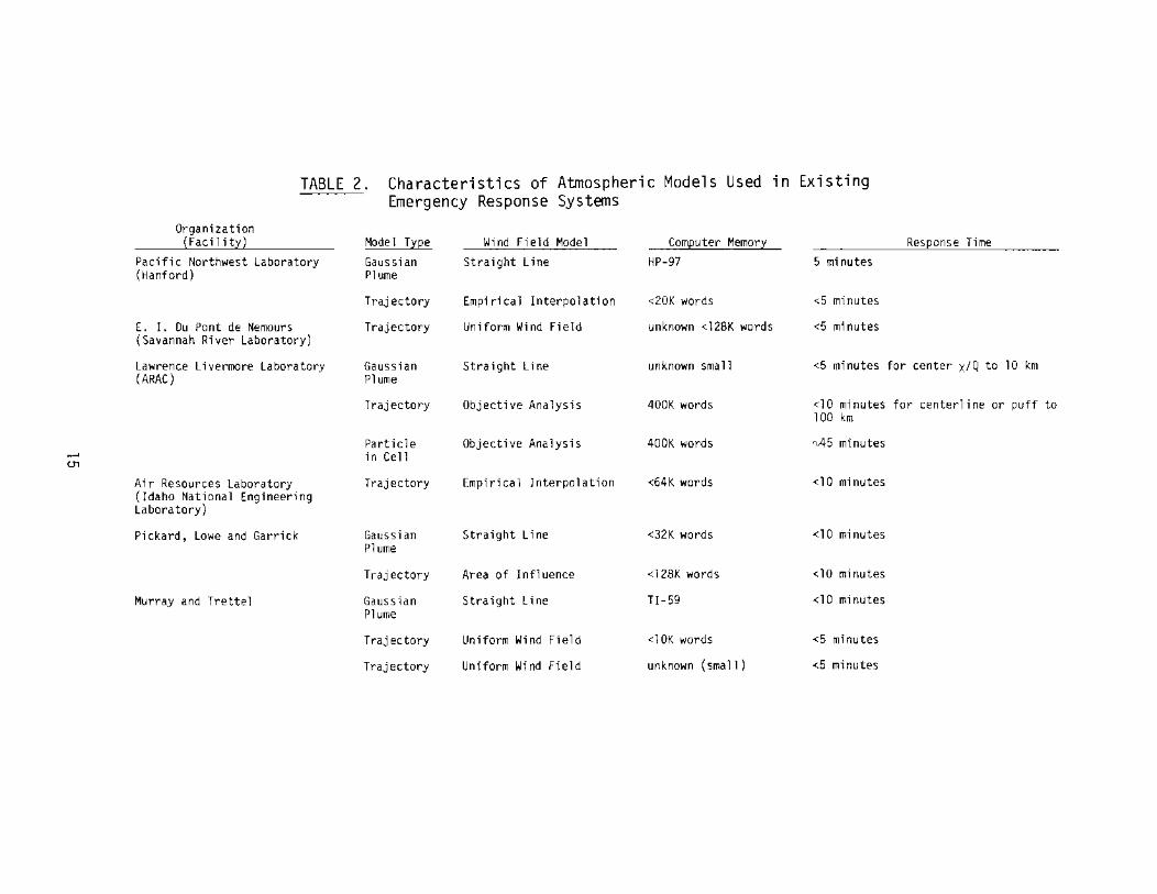
2. Characteristics of Atmospheric Models Used in Existing Emergency Response Systems

3. Common Word Sizes for Computers

4. Conversion of Number of Address Bits to Number of Addressable Memory Locations

5. Characteristics of Typical Computers

6. Estimated Computer Speeds

7. Comparison of Electronic and Electromechanical Memory Technologies

8. Categorization of Major Memory Device Types by Technology

9. Typical Costs and Access Times for Common Storage Devices.

10. Memory Cycle Times for Typical Computer Systems

11. Comparison of Data Transmission Techniques

12. Advantages of Low and High Level Programming languages

13. Factors Contributing to Computer System Reliability

14. Criteria for Determining Qualitative Maintainability Ratings for Computers

15. Classification of Factors Contributing to Reliability by Time Category

16. Adjustment Factors for Processor Failure Rates

17. User Ratings of Reliability Factors for Mini- and Mainframe Computers .

18. Estimated Failure Rates for Common Peripherals

19. Distributions of Minicomputer Computational Speeds

X j i i

14

15

19

19

20

22

24

25

25

27

41

43

45

47

49

53

54

56

64

20. Availability of Memory Features that Enhance Computer Reliability 64

21. Summary of Advantages and Disadvantages of Sources of Peripheral Equipment 65

22. Auxiliary Storage Devices Availability 65

23. Terminal Availability 66

24. List Prices for Minicomputers 67

25. Reported Frequencies of Early and Late Delivery of Computer Systems and Software by Computer Model 68

26. Reported Frequencies of Early and Late Delivery of Computer Systems and Software by Vendor . 68

xiv

INTRODUCTION

The Nuclear Regulatory Commission requires licensees to develop and main­tain an emergency response capability that includes assessment of the conse­quences of accidental releases of material to the atmosphere. Guidance for completion of this task is provided to licensees in several NRC documents including NUREG-0654 and NUREG-0696. The purpose of this report is to provide the NRC staff involved in reviewing licensee emergency response plans with background information on minicomputer systems for potential use in the collec­tion and dissemination of meteorological information related to the transport and diffusion of material released to the atmosphere.

Throughout this report we have identified computer components by name~ and we have assigned characteristics and capabilities to these components. we have also used the names of various organizations. This has been done to facilitate the discussion. The use of a name in the report does not carry with it an implicit or explicit endorsement of the organization, product or service. Simi­larly, the assignment of characteristics and capabilities to products and ser­vices does not constitute a guarantee or warrantee. The characteristics and capabilities presented are based upon advertising literature and published reports; they have not been subjected to independent tests.

This section provides an introduction to computer systems and computer system components. It contains definitions of terms commonly used in dis­cussions related to computers. The following section describes the treatment of meteorological information within the emergency response capabilities of four Federal nuclear facilities and two private environmental consulting organi­zations. The treatments described are representative of the current state-of­the-art in emergency response systems, but not necessarily the state-of-the-art in the implementation of compoter system capabilities. The last three sections of the main body of the report describe the capabilities, reliability and availability of available computer system components. Emphasis is placed on the identification of component features that might be useful in enhancing system performance in the transfer of information to decision makers. No attempt is made to define an optimum system. ~phasis is also placed on mini­computers; where possible, the capabilities and performance of minicomputers are compared with those of larger and smaller computers. Finally~ an appendix discusses models of atmospheric processes important in the evaluation of potential effects of releases of material to the atmosphere.

CO~lPUTER SYSTEMS

Computer systems are composed of hardware components and software com­ponents. The hardware components determine the ultimate system capabilities and limitations, and the software components provide the means for the develop­ment and utilization of the hardware capabilities. In an emergency response computer system, the hardware and software components should be selected to ensure t.hat the system is able to acquire, store, process and distribute information in a reliable, timely and effective manner.

1

HARDWARE COMPONENTS

A typical computer system is shown in Figure 1. The computer, itself, is composed of the central processing unit (CPU), the main memory and peripheral controllers. Peripheral devices linked to the computer in an emergency res­ponse system might include auxiliary storage devices, terminals, and displays, hard copy devices such as printers and plotters, and data acquisition systems. The dashed box in the figure indicates peripheral components generally located in relatively close proximity to one another. Remote peripherals are normally terminals, data acquisition systems, and printers and plotters.

The CPU includes an arithmetic unit, storage registers and a c'ontrol unit. It determines a number of the basic computer characteristics including: speed, instruction set and word size. The basic unit of information in a computer is the binary digit (bit). It has a value of either zero or one. A byte is a unit of computer storage capa~ity. frequently consisting of 8 bits. An 8 bit byte typically stores one character. {A minimum of 7 bits are required to stOre an American Standard Code for Information Interchange (ASCII) character.) Finally, a word is a set of characters treated as a single unit by a computer. A computer with 8 bit words treats each character individually, computers with 16 bit words treat 2 characters at a time, etc. word size is not a direct measure of a computer 1 s arithmetic precision.

~--- ------------------- ---1

I I

: ( AUX.'-, LOCAL PRI~! : STORAC~ TERMINAL

DATA :~T 1 I I

REMOTE ) ACQUISITION SYSTEM I I I I TERMINAL

I I

I I I

I PERl PHERAL ' I CONTROLLER' I

' I I I I I CENTRAL

I

' PROCESSING I

UNIT ' ' I I

MAIN I

MEMORY I I I

------------------------- _J

FIGURE l. Typical Computer System

2

The main memory of a computer provides online storage for instructions and data. The information stored in main memory is directly accessible to the CPU through the memory address at which the information resides. The maximum amount of directly addressable storage is determined by the CPU and the number of bits used to specify the memory address. Typically~ 8 bit word computers can address 64K bytes of memory. In computer applications K stands for 210 (1024), and M

20 stands for 2 (1~048~576). Because these numbers are near one thousand and one million~ respectively, K and Mare frequently translated to kilo- and mega-. Computers that use more than 16 bits for memory addresses or permit separation of memory into banks may be able to directly address 4M bytes of memory or more. In these computers other factors, including the cost of memory, limit memory size.

Peripheral controllers provide the interface between the CPU and the peri­pheral devices. The size of a computer system, in terms of number of peri­pheral devices, is limited by the number of controllers that can be attached to the CPU. Some controllers contain what are called general purpose ports that may be used to connect terminals, displays, printers, etc. These ports are either serial ports or parallel ports. In serial ports, information is trans­mitted sequentially, bit by bit, while parallel ports are used to transmit a number of bits of information (bytes or words) simultaneously. Serial ports are generally used if information is to be transmitted more than a few feet.

Computer terminals can be divided into two basic classes, interactive and batch terminals. Interactive terminals provide the user with the opportunity to communicate directly with the computer during execution of a program, whereas with a batch terminal the user submits a job to the computer and has no further role until the computer returns the results. Interactive terminals require both a keyboard for data input and a display for computer output. Common interactive terminals are video-display terminals (VDT) and teletype terminals. In a VDT the display is presented on a cathode ray tube (CRT) similar to a television screen. There is no permanent record of the output. Various other peripheral devices can be used to obtain permanent records of computer output when a VDT is used as a primary communications device between the user and the computer. Interactive execution of computer programs during an emergency has several advantages over batch execution. These advantages include error checking and immediate correction of erroneous input data prior to use by the program.

VDTs are frequently classified as "dumb," "smart" or "intelligent." This classification refers to data processing capabilities of the terminal. A dumb terminal is limited to transmitting, receiving and displaying information. An intelligent terminal may be a complete microcomputer with its own memory and is user programmable. A smart terminal falls between these extremes. It usually has some memory and a limited processing capability, but it is not user programmable.

The local terminal shown in Figure 1 may be dumb, smart The remote terminal may also be dumb, smart or intelligent. sary for the local and remote terminals to be identical.

3

or inte11 igent. It is not neces-

Auxiliary storage devices are included in computer systems to permit online storage of data and programs for immediate use by the computer. The principal auxiliary storage devices are magnetic tape units and disk units. Both types of devices provide storage capacities far exceeding the capacity of a computer's main memory. They also use recording media that can be removed from the system, which facilitates archiving input data and computer output. Disk units provide significantly faster access to data than is available with tape units.

The printer shown in Figure 1 is representative of several types of devices that can be connected to a computer to provide permanent records of computer output. Other devices that fall into this category include plotters and units that make direct copies of VDT displays.

The computer system components discussed thus far are generally located in relatively close proximity to one-another. As a result, they can be connected with minimal interfaces. When remote components are added to the system, for example, the remote terminal and data acquisition system shown in Figure 1, communications interfaces become more involved. Communications protocols, transmission media and transmission speeds need to be established. A com­munications protocol is a set of rules governing data transmission. It includes a description of the hardware connections, the type of transmissions, and the method of encoding the information.

long-range data transmissions are generally made using analog signals rather than the digital signals used within the computer. Thus, most data transmission systems use modems. The modem at the transmitting station receives digital information from the computer or terminal and uses the digital informa­tion to modulate an analog signal. The modulation can be in the frequency, amplitude or phase of the signal. Frequency modulation is most common. At the receiving station, a modem converts the analog signal to digital form for use by local devices.

Data transmission media include telephone lines, dedicated wires, fiber optics, and radio and microwaves. The medium chosen depends, to a large extent, on the distance involved, the environment, and the frequency of data transmissions.

The term baud is sometimes used to describe the speed at which data are transmitted. The baud rate is the number of bits transmitted per second. The bits transmitted include: bits in characters, bits used to indicate the begin­ning and end of each character and message block, and bits used to provide a means for detecting transmission errors. For many data transmission systems, the data transmission rate in characters/second is approximately one tenth the baud rate.

The last peripheral shown in Figure 1 is a data acquisiti?n syste~. Oat~ acquisition systems receive signals from sensors and make the 1nformat1on avall­able as required. They may also process the signals and store th~ ~r?cessed information. Initial processing of sensor signals by a data acqu1s1t1on

4

system reduces both the computational load on the main CPU and the traffic that must be handled by the communications sytem. Addition of memory and an on­demand data transmission capability to an acquisition system increases its flexibility and improves its reliability.

SOFTWARE COMPONENTS

Computer system software components include: the computer operating, system, the programming language, and the user applications programs. Although these components are not as substantial as the hardware components, they may represent a significant portion of the total system investment.

The computer operating system is a set of routines that controls the com­puter system. It provides the interface between the user's programs and the computer hardware. Multi-user, multi-tasking operational systems for minicom­puters and some microcomputers permit a single computer system to process several programs simultaneously. However, the apparent speed of the computer may decrease as the number of tasks undertaken simultaneously increases.

The set of instructions used by a programmer is a programming language. Common languages used in scientific applications include: FORTRAN, BASIC and PASCAL. Before any language can be used with a computer system, the language must be implemented on the system. That is, the computer system must have access to the compilers and interpreters that can translate the programming language instructions into machine language instructions. The apparent compu­ter speed is a function of the programming language used. FORTRAN programs execute more rapidly than BASIC programs, and PASCAL programs tend to be faster than FORTRAN programs, given the same task.

Once a computer system has been selected, an operating system and program­ming languages can be selected from available options. It is not necesary to develop or modify them for each specific application. On the other hand, user applications programs are likely to be developed or modified for each specific application. User programs, in emergency response applications, can be roughly divided into programs used to manage the base of available data, and programs that use the data to estimate impacts. Programs in the latter group generally involve models of real environmental processes and fix minimum requirements for hardware capabilities. Various approaches to modeling atmospheri-c processes are described in the Appendix.

5

METEOROLOGICAL INFORMATION HANDLING IN EXISTING EMERGENCY RESPONSE SYSTEMS

Having introduced computer systems we will now show how they are used in emergency response applications. This section describes the acquisition, analy­sis and dissemination of meteorological information by six organizations that provide meteorological services for nuclear facilities. Four of these organi­zations, Pacific Northwest Laboratory, Air Resources L'aboratory, Lawrence Liver­more Laboratory and E. I. DuPont de Nemours and Co., provide meteorological services for Federal nuclear facilities. The other two organizations, Pickard, Lowe and Garrick, and Murray and Trettel, provide meteorological services for utilities that operate nuclear power plants. The services to be described were generally developed over a period of time prior to the publication of NUREG-0654. As a result, they were not designed specifically to meet its require­ments. However, the services are typical of existing methods for handling meteorological information in emergency response applications.

PACIFIC NORTHWEST LABORATORY (Hanford)

The Atmospheric Sciences Department of the Pacific Northwest Laboratory provides meteorological services for Hanford. The majority of the department staff is engaged in research, but the department also has a full-time forecast staff. The forecast staff has the responsibility of evaluating the transport and diffusion of material released to the atmosphere in the event of an accident.

When the forecast staff is notified of an actual or potential release, it uses an interactive Lagrangian-trajectory, puff diffusion model (Ramsdell and Athey, 1981) to predict plume positions and estimate exposures in affected areas. The model is run on a UNIVAC 1100/44 computer and requires less than 20K words of memory. Initialization of the model takes about 2 minutes. The results of the model simulation for the first hour's release are available to the forecasters within 30 seconds of completion of model initialization. A full 12 hours simulation can be completed in less than 3 minutes following initialization. This time includes the time required to display model output for forecaster evaluation at the end of the first, second, sixth and twelfth hours. Model output is displayed on thP. forecaster's VDT. and may also be routed to one or more printers. Clear plastic overlays are used to add geo­graphical and demographical information to the computer printout.

The Lagrangian-trajectory, puff diffusion model uses a series of puffs to simulate a continuous plume. The centers of mass of the puffs are advected in a spatially and temporally varying wind field derived from measured or forecast winds. Diffusion about each puff's center-of-mass is a function of distance from the release point and atmospheric stability. A more detailed discussion of atmospheric models is presented in the Appendix.

7

Meteorological data for use with the model are obtained from observations at the Hanford Meteorological Station (HMS) and from wind sensors located throughout the Hanford Area. Data from the outlying wind sensors are relayed to the HMS using radio telemetry and data acquisition system built around a PDP ll/05 minicomputer. Regional and national weather information is available to the forecasters through the National Weather Service AFOS system. The AFOS station utilizes a Data General Eclipse 230 minicomputer.

The observed meteorological data and forecasts are entered into data files maintained on the UNIVAC computer system disks for use by the transport and diffusion model. Observed data are entered each hour, and forecasts are entered every 8 hours or when revisions become necessary. The entry of this data into the disk files is a manual operation.

As a backup to the trajectory model, the forecasters have a Gaussian plume diffusion model that runs on a Hewlett-Packard 97 programmable calculator. The model provides exposure estimates at plume centerline as a function of distance from the source, wind speed and atmospheric stability. The transport is impli­cit in the model and assumes that the material will be carried with the wind in a straight line away from the source. Neither spatial nor temporal variability of meteorological conditions are treated in the model.

AIR RESOURCES LABORATORY (Idaho National Engineering Laboratory)

Meteorological services at the Idaho National Engineering Laboratory are provided by the National Oceanic and Atmospheric Administration 1 s Air Resources Laboratory, Idaho Falls Field Office (ARL). The primary function of the field office is research; however, in the event of an emergency the staff of the field office would provide the atmospheric transport and diffussion estimates needed for use in responding to the emergency.

The ARL staff uses a Lagrangian trajectory puff model to make transport and diffusion estimates. The model has been derived from the model of Start and Wendell (1974), as was the PNL model, and is implemented on Interdata (now Perkin-Elmer) 7/16 and 7/32 minicomputers. Model results are output via a graphics VDT and a hard-copy device that provides permanent records of selected display presentations. They are available within 10 minutes of the start of model simulation. Model output products include: geographical plots of the wind field, trajectories of the centers of mass of puffs, and exposure estimates. During off-hours, there may be a delay of an hour or more in obtaining model output if it is necessary to call in the staff and start up the computer system. If the computer system is running, the model can be run remotely from a terminal downtown in Idaho Falls.

Meteorological data for use with the model are obtained from an array of wind sensors. There are two independent wind systems. The first system uses radiotelemetry to relay the data to the base station where they are recorded on magnetic tape and are available for use by the models. The other system uses telephone lines to relay the data to strip chart recorders at the base

8

station. If it becomes necessary to use the data from this system in the model, the data must be manually entered into computer files. These data may be supplemented with data obtained through special meteorological observations on site and with National Weather Service data that are available at ARL.

The minicomputers in the system have been used in field installations in poor computer environments without air conditioning or filtration, and have proven to be extremely reliable.

LAWRENCE LIVERMORE NATIONAL LABORATORY (ARAC)

The Atmospheric Sciences Division staff of Lawrence Livermore National Laboratory is engaged in research; however, in an emergency they can be called upon to provide atmospheric transport and diffusion estimates for the Depart­ment of Energy. These estimates are provided through the Atmospheric Release Advisory Capability (ARAC) developed by LLNL. ARAC's services are also pro­vided to the Federal Aviation Administration. Products of the ARAC models include: instantaneous and integrated air concentrations, ground-level doses, and individual exposures.

Major components in the ARAC system include: a terminal at the site of an emergency, and the ARAC Center and the computer facility at LLNL in Livermore, California. The remote terminal at the site of the emergency is used for com­munication with the ARAC Center. Data from the vicinity of the emergency are transmitted to the center, and the results of the model computations at Liver­more are sent to the site. This communications system is based upon Digital Equipment PDP 11(40 and PDP 11/4 minicomputers, and uses telephone lines to connect the remote terminal and the Center. Data transmissions take place at 300 baud.

At the ARAC Center, the Center staff takes the information from the site of the emergency, meteorological information from the National Weather Service and the Air Force Global Weather Center, and topographic information from their own files and runs several transport and diffusion models. The models used range from simple Gaussian Plume models to large particle-in-cell models. The particle-in-cell models are run on the CDC 7600 computers at the LLNL computer center; the other models are run on a Digital Equipment VAX 11/780 super­minicomputer at the ARAC Center.

Particle-in-Cell (PIC) transport and diffusion models are more complex than the Lagrangian-trajectory, puff diffusion models. PIC models use a large num­ber of particles to simulate the release. The movement of particles is com­posed of a mean component determined by the particle's position and a random component. Both the motion of the particle and the wind field are three­dimensional. Concentration in the plume is proportional to the number of particles in a given volume (cell). The MATHEW/ADPIC models in the ARAC suite requires about 400K words of CDC 7600 memory.

9

Initial results can be expected from the models run on the VAX 11/780 within 10 minutes. It takes considerably longer to obtain results from the models run on the CDC 7600s. Some of the additional time is the result of the size and complexity of the models, and some of the additional time results from administrative procedures required for security reasons. If the topographic information is required by a model and is not immediately available to the computer, several hours are required to prepare the topographic file. If the required topographic information is available, output from MATHEW/ADPIC can be obtained in about 45 minutes.

Response time of the ARAC system is about 15 minutes during normal working hours. During non-working hours, the time required for the initial response of the ARAC system may be an hour and a half to two hours. The additional time represents the time required to assemble the necessary staff for the ARAC center.

E. I. OU PONT DE NEMOURS (Savannah River Laboratory)

The Savannah River Laboratory has a highly developed emergency response capability that includes an emergency operations center (EOC) that is manned at all times. Meteorological support for the EOC staff is provided by the Atmos­pheric Sciences research staff of E. I. DuPont de Nemours through a micro­computer system. The research staff works normal hours, but meteorological information is available at all times through a remote terminal located in the EOC. The information available includes area maps, wind and temperature data, and transport and diffusion estimates. A hard copy device is included with the terminal in the EOC to allow the EOC staff to make copies of terminal display as appropriate.

Minicomputer technology was selected for the system because of its relia­bility. Currently the system is built around a POP-ll/40 computer with a 128K word memory. Backup power is available for the computer system to permit its use in the event of a loss of normal power. A larger IBM computer is avail­able at SRL, but it is not included in the emergency response system because it can not be dedicated to that use and because it is less reliable than the microcomputer.

The computer programs in the system are all interactive; the users are provided with menus that list the available programs and program options. When user input is required, the programs prompt the user, clearly indicating the needed information. Transport and diffusion estimates are made using Gaussian plume and puff trajectory models. Onsite and near-site meteorological data are obtained from disk files prepared by the data acquisition programs that run continuously on the minicomputer. The trajectory model uses a uniform wind field to estimate plume transport. As a result, any curvature in the trajec­tories is induced by temporal variations in the wind rather than spatial varia­tions. The wind speed and direction used in the trajectory mode are averages computed from the observed directions and speeds reported in the vicinity.

10

Diffusion within the puffs is computed using measured standard deviations of wind direction and elevation. Output of the interactive models is available at the EOC within 10 minutes. More sophisticated models are available to the Atmospheric Sciences staff, and are run on the IBM computer.

The PDP-11 computer controls the meteorological data acquisition system in addition to its other functions. Wind and temperature measurements are made at 2Hz and are used to compute 15 minute averages which. are stored in disk files for model use. The onsite meteorological data are supplemented by wind fore­casts prepared for SRL twice each day by Techniques Development Laboratory of NOAA. The forecasts cover thirty hour periods and are manually entered into the system.

PICKARD, LOWE AND GARRICK

Pickard, Lowe and Garrick (PLG) provides environmental consulting services to utilities. Among the services offered are meteorological data acquisition and analysis specifically designed to meet NRC requirements for licensing and operat­ing nuclear facilities. For emergency response, PLG has developed a system that consists of four main components: an onsite minicomputer, a central data analy­sis computer, a remote terminal in the PLG office, and a remote terminal in the power control room.

The onsite minicomputer is a Varian/Sperry UNIVAC V77-800 computer with analog to digital signal conversion capability and 32K words of memory. It is used for data collection and storage. Wind and temperature data are collected at 10 second intervals and used to form 15 minute averages of wind direction, wind speed, temperature, temperature difference and dew point. These averages are relayed to the central station every 4 hours using phone lines, although the data may be obtained more frequently if necessary.

The central station is a UNIVAC V76 computer located at Rockville, Mary­land. During routine operations the computer is used for a variety of tasks, but in the event of an emergency it can be dedicated to processing data related to the emergency. A data file, containing 15 to 45 days data, is maintained on disk at the central computer. Every month the most recent month•s data are copied to magnetic tape for archiving.

Data analysis programs available on the V76 computer include Gaussian plume and segmented plume trajectory models for estimating transport and diffusion. The trajectory model uses an area of influence wind field. Approximate memory requirements of the models are: 32K words for the Gaussian plume model, and 64K words for the trajectory model.

System operation is controlled and data analysis programs are run from a remote graphics terminal in the PLG office. Through this terminal, the PLG staff can examine the meteorological data in raw or summarized form, obtain tables of normalized concentrations and exposures, and obtain plots showing

11

normalized concentration or exposure isopleths on maps showing topographic fea­tures and political subdivisions. All programs are run interactively~ and the time required to complete model initialization and obtain the output is less than 10 minutes. A hard copy unit is connected to the terminal to permit the staff to make permanent copies of the computer output when appropriate.

The control room terminal is similar to the terminal in the PLG office. Its purposes are to provide the reactor operators with direct access to the meteorological data and to permit the operators to receive information from the PLG offices following a release. The transport and diffusion models can be run from the control room.

The reliability of the system is reported to be in the go to 95 percent range, with the onsite minicomputer reliability exceeding 95 percent. Backup power is not provided for either the central computer or the terminal in the PLG office.

MURRAY AND TRETTEL

Murray and Trettel (MT) is a meteorological consulting firm with a staff of research scientists and forecasters. The list of services that they provide to clients includes: operational forecasts, air quality and dispersion model­ing studies, and nuclear emergency support. As an integral part of these services, MT has developed extensive capabilities in data acquisition and analysis.

Murray and Trettel has been using microprocessor-based data acquisition systems since 1974. Their onsite systems include memory for temporary storage of the data and auto-answering modems to facilitate transfer of data from the measurement site to data files on the computer system at the MT offices. Data transfer takes place via phone lines. The data acquisition systems operated on ac power are provided with backup power sources, and those systems operating on de power use have noninterruptable power supplies. A data recovery rate of about 99 percent has been achieved with the systems by routinely calibrating the instruments, monitoring instrument performance on an hour-to-hour basis, and immediate response when an instrument failure is suspected. The factor causing the greatest data loss is lightning, which may damage several instru­ments at one time.

Several levels of data processing capability exist at MT. Primary compu­tational power is provided by Texas Instruments (TI) 9808 and 990/12 minicom­puters. Transport and diffusion models are run on a TI 99/4 microcomputer. A plume segment trajectory model that occupies less than lOK words of memory is one of the models available. It predicts the trajectories of plume segments for periods of up to 36 hours. Each segment represents one hour of release. Program output consists of the endpoints of each segment, the normalized con­centration at the segment centerline and plume width at the downwind end of the segment. Trajectories plats are also available. The models on the

12

TI 99/4 are backed up by a Gaussian plume model program that runs on a TI 59 handheld calculator and detailed set of instructions on the operation of the TI 59 program. The ultimate backup capability is provided by the forecasting ability of the MT forecast staff. Two members of the forecast staff are on duty at all times.

Reactor control room operators have direct access to the meteorological data collected onsite and to the meteorological forecasts prepared by MT. Transport and diffusion information is relayed to the operators by the MT staff, and is available within 10 minutes of the time MT is notified that there is an emergency.

SUMMARY AND COMPARISON OF METEOROLOGICAL RESPONSE CAPABILITIES

The meteorological aspects of emergency response capabilities of four Fed­eral nuclear facilities and two private environmental consulting organizations are summarized in Tables 1 and 2. These responses appear to be representative of the state-of-the-art. The prime emergency resource of each of these capabi­lities is the staff of the organization providing the meteorological service. In each case, the staff includes atmospheric scientists specializing in trans­port and diffusion.

The computational hardware resources listed in Table 1 are generally mlnl­computers. Only PNL and LLNL rely to any extent on large mainframe computers. The Hanford reliance is primarily due to computer availability, and the LLNL is due to model requirements. The characteristics of atmospheric transport and diffusion models currently incorporated in emergency response capabilities listed in Table 1 are summarized in Table 2. The models tend to be relatively simple models based on Gaussian assumptions. Computer memory requirements listed in Table 2 are a reflection of the modest size of typical models.

The data acquisition capabilities of the various organizations do not appear to vary significantly. All can make use of telephone lines and radio or microwave telemetry. In addition, National Weather Service data is routinely available to all organizations.

The final characteristic summarized in Table 2 is response time. Each organization has a capability to respond with transport and diffusion estimates in less than 10 minutes once it is operationally involved in an emergency. However, not all of the organizations provide for full time staff availability. Only E. I. Du Pont and Pickard, Lowe and Garrick provide users with access to transport and diffusion estimates without initial evaluation by atmospheric scientists, and of the other 4 organizations, only PNL and MT have full time staff availability. In the event of an emergency during off hours there may be significant time lost while appropriate staff members of the remaining organi­zations are called in.

13

""

TABLE l • Typical Existing Meteorological Capabilities for Emergency Response

Organization --~(~F~oo,i, 1 ity)

Pacific ~1ortl1west Laboratories (f-lanford)

E. I. Ou Pont de Nemours (Savannah River Labor·atory)

Lawrence Livermore Laboratory (ARAC)

Air Resources laboratory {Idallo National EngirJeering Laboratory)

Pickard, Lowe and Garrick

Murray and Trettel

Staff

Atmospheric sciences re­search staff, full time forecast staff

Atmospheric sciences re­search staff normal working hours, on call off hours, no forecast staff. Full time emer­gency operations center

Atmospheric sciences re­search staff, nonnal working hours, on call off hours, no forecast staff

Atmospheric sciences re­search staff normal work­ing hours, on call off hours, no forecast staff

Staff of engineers and atmospheric scientists. 2 shifts per day, no forecast staff

Atmospheric research/ consulting staff normal working hours, forecast ~taff full time, two forecasters/shift

Com12_uters

UNIVAC 1100, HP-97 backup

Dedicated PDP 11/40, IBM 360/ 195 available, ARAC terminal available

CDC 7600 (4) not dedicated, without backup power sources, VAX 11/780, PDP ll/40, POP ll/4

Interdata 7/15 (3) and 7/32 (1)

UNIVAC V75 (operated by Digi­tal Graphics, Inc. but can be committed 100% in an emergency)

Texas Instruments 980B, direct access to available data and forecasts. Tl 99/4 microcom­puter backup, followed by TI 59 calculator programmed for x/Q, 11 990/12 for development work

Data Acquisition

PDP 11/05 based radiotelemetry system for surface winds at 22 on- arod near-site loca tions, 400ft instrumeroted tower, pilot balloons, acoustic sounder, National Wea­ther Service, AFOS.

Data from 7 surface wind sensors hardwired to PDP ll/40, instrumented 1500 ft TV tower near site, National Weather Service data, twice daily 30 hour wind forecasts from NOAA Technique Development Laboratory

Local data by telemetry, National Weather Service data, Air Force Global Weather Central, supplementary data as available.

2 independent systems, 1 primarily radio­telemetry, the other telephone lines pro­vide wind data in the 50-150ft elevation range. Special surface and upper air observatioris in emergency. National Wea­ther Service data.

Onsite systems using Sperry-UNIVAC V77-800 computers, data relay to central computer via telephone lines, automatic dialup/ answering modems

Texas Instruments microcomputer data acquisi­tion systems with auto answer modems, backup power for systems. Data from numerous power plant sites in Mid-West. National Weather Service data

-~

TABLE 2. Characteristics of Atmospheric Models Used in Existing Emergency Response Systems

Organization (Facility)

Pacific Northwest Laboratory (Hanford)

E. 1. Du Pont de Nemours (Savannah River Laboratory)

Lawrence Livermore Laboratory (ARAC)

Air Resources Laboratory (Idaho National Engineering Laboratory)

Pickard, Lowe and Garrick

Murray and Trettel

Mode 1 Ty~e

Gaussian Plume

Trajectory

Trajectory

Gaussian Plume

Trajectory

Particle in Cell

Trajectory

Gaussian Plume

Trajectory

Gaussian Plume

Trajectory

Trajectory

Wind Field Model

Straight Line

Em pi rica 1 Interpolation

Uniform Wind Field

Straight Line

Objective Analysis

Objective Analysis

Empirical Interpolation

Straight Line

Area of Influence

Straight Line

Uniform Wind Field

Uniform Wind Field

Comeuter Memory Response Time

HP-97 5 minutes

<20K words <5 minutes

unknown <128K words <5 minutes

unknown small <5 minutes for center x_/Q to 10 km

400K words <10 minutes for centerline or puff to 100 km

400K words o..45 minutes

<64K words <10 minutes

<32K words <10 minutes

<128K words <10 mirwtes

TI-59 <1 0 minutes

<lOK words <5 minutes

unknown (small) <5 minutes

COMPUTER CAPABILITIES

This section discusses computer capabilities. The system components cov­ered are:

• Computers complete with memory, operating system and programming languages.

• Auxiliary mass storage devices including disk and magnetic tape drives.

• Terminals with manual data entry capabilities and displays.

• Hard copy output devices including printers, plotters and display copiers.

• Communications systems capable of interfacing with remote data acquisi-tion systems and other computers.

We will not discuss data acquisition systems or applications programs. The dis­cussions will be generic in the sense that our goal is to identify available components and their characteristics. A good portion of the material involves definition of terms that occur frequently in discussions of computer systems. Particular emphasis is given to minicomputers' capabilities.

This section is not the result of a rigorous computer system design pro­cess. As a result there is no attempt to determine compatibility between indi­vidual components. However, once a suitable computer is selected it should be possible to find compatible peripheral devices of each type. But it is not reasonable to expect to successfully assemble and operate a system of inde­pendently and arbitrarily selected components. An emergency response computer system does not need to be separate from other computer systems, although for purposes of the current discussion we will assume that it is. When a proposed computer system includes components from several sources, component compatibil­ity should be demonstrated rather than assumed.

COMPUTERS

Computers perform the following functions:

• computations and logical operations • control of hardware operations • storage of instructions, addresses and data • interconnection between devices.

The organization of computer components is called the computer architecture. It influences computer performance, programming ease, ease of connecting peri­pherals and cost.

17

Within the computer, the central processing unit (CPU) performs the compu­tations, has registers for local storage of instructions, addresses and data, and controls hardware operation by executing instructions. It is supported by the main or primary memory, a clock to synchronize computer operations and a power supply. The CPU is controlled by a computer operating system (OS) that schedules tasks, manages resources including allocating memory and manages data transfer and communications. The OS may also include utility software such as text editors. It acts as an interface between the user's programs and the computer.

If the terms micro-, mini- and mainframe(a) computer have any practical significance, the significance relates to the CPU. The connotations of these relative terms are generally associated with capabilities such as speed, number of users, peripherals and languages supported, etc., as well as with physical size, power consumption and cost. In many cases it is no longer possible to clearly distinguish between classes. For example, the DEC PDP-11 line of computers has undergone significant evolution since the introduction of the PDP-11/20 minicomputer in 1970. Technological advances have permitted DEC to produce a series of computers of comparable capability at decreasing prices. This series includes the PDP-11/23 that has an LSI 11/23 CPU. The LSI 11/23 CPU is available in computers by other vendors that are termed microcomputers. Going the other direction, DEC produced a series of POP-11 computers that includes the PDP-11/70 and VAX-11/780 computers. The capabilities of these computers significantly exceed those normally associated with minicomputers. The VAX-ll/780 capabilities are comparable with those of recent generation mainframes. Further evidence of erosion of the clear-cut distinction between computer classes is provided by IBM's recent development of a single inter­grated circuit that duplicates the CPU of its System/370 model 168 processor.

Computers should be selected and evaluated in terms of specifications directly related to their intended functions without the use of references to class. It is unlikely that the terms microcomputer, minicomputer, etc. will fade from use or lose their connotations in the near future. However, the foregoing paragraph is sufficient to demonstrate that these terms must be treated as qualitative indicators of computer characteristics in a multi­dimensional continuum. One or more characteristics of a specific computer may deviate significantly from those inferred from the normal class connotation. We will continue to refer to computer classes with this understanding.

The number of CPU registers and their usage contribute significantly to characteristics of a computer. They determine word size and addressing capabil­ity of the system. Table 3 gives typical word sizes for micro-, mini and main­frame computers. There is a tendency to use word size as an indicator of system capability. However, other factors are sufficiently important that the best policy is not to trust this tendency.

(a) Mainframe is commonly used to indicate large computers; however, it can also be used to indicate the portion of the computer that contains the CPU.

18

TABLE 3. Common Word Sizes for Computers

Microcomputers

Minicomputers Mainframe Computers

Common Word Sizes (bits)

8' 16 8, 16, 32

36, 60, 64

The ability of a computer to address locations in memory is mined by the number of bits (binary digits) used for addresses. n address bits can address 2n locations. It is not necessary for integer multiple of the word size, however, it is usually an even version from address bits to maximum number of locations is given The ultimate limit on addressable memory on many minicomputers is utility of additional memory increments.

TABLE 4. Conversion of Number of Address Bits to Number of Addressable Memory Locations

Addressable Address Bits Memor,t Locations

10 lK 12 4K

14 16K 16 64K 18 256K 20 1 024K 22 4096K

directly deter­A computer with

n to be an number. Con­in Table 4. the cost and

Computer word size is frequently used as an indication of computer arith­metic precision. Again, it is not a true indicator. Precision is determined by the representation of the numerical values within the computer. Specifi­cally, it involves the number of words assigned to each numerical value, the word size and the uses of the available bits. For integers, all bits are used to determine magnitude, and if m bits are available, the integer range is

[+2m-l - 1]. Precision in floating point numbers depends on the distribution of the available bits between a mantissa and a characteristic. Increasing tne number of bits in the mantissa simultaneously increases precision available and decreases the maximum absolute numerical value that can be represented. As a result, system design requires a compromise between precision and range.

High- level programming languages provide the user with some flexibility in selectinq arithmetic precision by permitting the user to control the number

19

of words assigned to each numerical value. Double precision in FORTRAN and the long variable type in some versions of BASIC are examples of this control.

Table 5 presents word size, addressable memory and numerical prec1s1on limits for several typical computers. Northstar and Cromemco are microcompu­ters; the PDP-11 's are minicomputers; the UNIVAC and CDC are mainframes, and the VAX-11 is in a gray zone between minicomputer and mainframe. The numerical limits in the table are those for FORTRAN, except for the Northstar. For the Northstar, the limits are for Northstar BASIC, which does not have an integer variable type.

TABLE 5. Characteri sties of Typical Computers

Addressable Floating Point Precision Word Size Memory Largest (decimal digits)

Com~::~uter (bits) (Words) Integer Single Double

NORTHSTAR 8 64K 8 14

CROMEMCO 8 512K ±215 -1 7 16

PDP-11/20 16 32K ±231_ 1 7 16

PDP-ll/45 16 128K ±231_, 7 16

VAX-11 /780 31 ±231_1 7 16

UNIVAC 1100 36 256K :!.235 -1 8 18

CDC CYBER-74 60 ±259 -1 14 29

The table shows that the smaller computers are capable of supporting large memories and demonstrates the problem of estimating memory from word size. The internal architecture of the two microcomputers is similar. Both systems are based on the Z80 microprocessor. and they use the same bus struc­ture. The difference in addressing capability comes from a bank select cap­ability incorporated in the Cromemco that allows the user to select any one of eight 64K word memory banks. This selection can be made, and changed, within a program. Similarly, the PDP-11 computers have the same number of address bits, but two of those bits are not available to the user in the PDP-11/20.

From Table 5 it is possible to determine the number of words useU to represent numerical values in each of the computers. For 8 and 16 bit word computers, integers are represented by two words. While for computers with 32 bit or larger words, integers are represented by a single word. Similarly, microcomputers assign 4 words to floating point variables and the minicompu­ters assign 2 words. The larger computers assign one word to each variable. Thus, all of these computers use at least 32 bits to represent floating point numbers. With the exception of the CYBER-74, they have similar floating point precision.

There is much greater variability between computers in computational speed than there is in arithmetic precision. Comp~ter speed can be estimated

20

in two ways. or it can be

It can be estimated directly from the estimated using benchmark programs.

computer specifications,

Estimating speed from specifications starts by determining the time required for the processor to complete each individual type of instruction. The speed of the computer is then estimated from a weighted average of the individual instruc­tion times. Weitzman (1980) and Longbottom (1980) discuss estimating computer speeds in this manner.

Factors affecting individual instruction times are:

• processor cycle time • number of operations required to complete the instruction • locations of the operands, if any • memory cycle time if memory access if required.

The weighting used in determining the average instruction time is a function of the type of program being simulated. For example, the weights for estimating computer speed for a process control application would be different from those used to estimate speed for a computer to be used in modeling atmospheric trans­port and diffusion. Therefore reported speeds must be considered typical rather than exact values. Computer speed estimates are reported in KIPS (thousand instructions per second) or MIPS (million instructions per second).

Table 6 shows estimated speeds for several systems ranging from microcom­puters to super mainframe computers (CDC-7600 and CRAY-1). If the super main­frames are excluded from the table, the speeds range from 0.3 to 18 MIPS for microcomputers, minicomputers and the standard mainframes. The fastest of the remaining computers are the MIPROC 16, a microcomputer, and the AP-190L, a minicomputer. Both of these computers are special arithmetic processors that can be interfaced with host mainframe and minicomputers. The remaining entries in the table indicate that a typical range of speed differences between micro and minicomputers and mainframes might be an order of magnitude. Differences between specific systems in specific applications could be significantly more or less.

Benchmark tests provide the second measure of computer speed. They are better at giving speeds of computers relative to one another than they are at estimating the speed of a computer in terms of KIPS or MIPS. A benchmark test consists of running a common (or as nearly common as possible) benchmark program on several computers and then comparing execution times. Because the benchmark program is a mix of instructions, the relative rankings of computers within a group may vary from one benchmark test to the next.

Conti (1978 and 1979) describes problems encountered in developing standard benchmark tests in detail. These problems shed light on the limitations inher­ent in the benchmark process. It is instructive to briefly consider some of these limitations because they arise in evaluation of computer efficiency without actually delving into the internal structure of the processors and instruction sets.

21

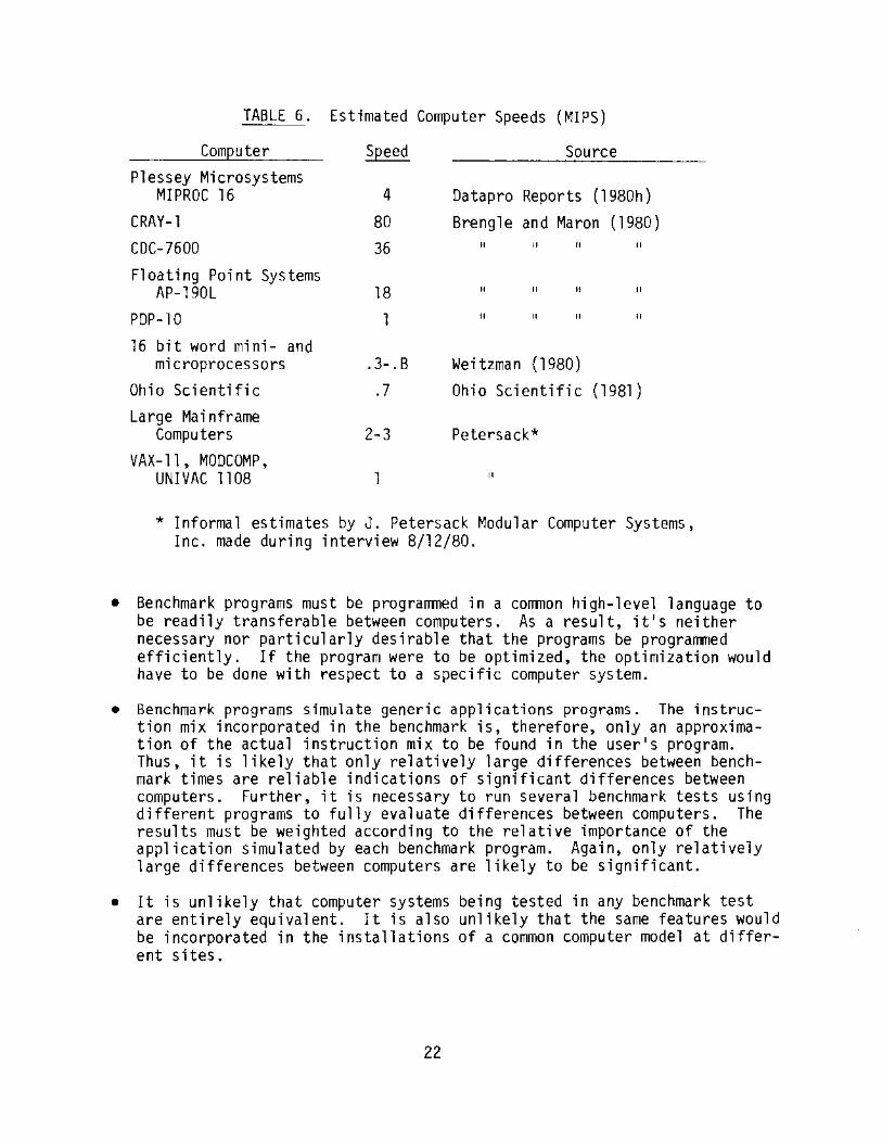
TABLE 6. Estimated Computer Speeds (MIPS)

Computer Plessey Microsystems

MIPROC 16

CRAY-1 COC-7600

Floating Point Systems AP-190L

PDP-10 16 bit word mini- and

microprocessors Ohio Scientific Large Mainframe

Computers VAX-11, MODCOMP,

UNIVAC 1108

Speed

4 80 36

18

1

.3-.8

.7

2-3

1

Source

Datapro Reports (198Dh) Brengle and Maron (1980)

• •• • • •

• •• • ••

•• • •• • •

Weitzman (1980)

Ohio Scientific (1981)

Petersack*

••

* Informal estimates by J. Petersack Modular Computer Systems, Inc. made during interview 8/12/80.

• Benchmark programs must be programmed in a common high-level language to be readily transferable between computers. As a result, it 1 s neither necessary nor particularly desirable that the programs be programmed efficiently. If the program were to be optimized, the optimization would have to be done with respect to a specific computer system.

• Benchmark programs simulate generic applications programs. The instruc­tion mix incorporated in the benchmark is, therefore, only an approxima­tion of the actual instruction mix to be found in the user 1 s program. Thus, it is likely that only relatively large differences between bench­mark times are reliable indications of significant differences between computers. Further, it is necessary to run several benchmark tests using different programs to fully evaluate differences between computers. The results must be weighted according to the relative importance of the application simulated by each benchmark program. Again, only relatively large differences between computers are likely to be significant.

• It is unlikely that computer systems being tested in any benchmark test are entirely equivalent. It is also unlikely that the same features would be incorporated in the installations of a common computer model at differ­ent sites.

22

• A benchmark program is designed to provide information on the relative performance of computers on a common set of instructions. It is not necessarily designed to determine the actual time required to complete the task nominally assigned. The program may not be written to complete the underlying algorithm in an efficient manner. The algorithm itself may not even be an efficient method of completing the task. Neither of these factors has a significant bearing on relative comparisons between computers if a ranking is desired. If benchmark results are interpreted to give real execution times for a specific application, undue significance may be given to the differences.

Recent issues of Interface Age provide an excellent example of the use and problems associated with a benchmark test. Fox (1980) gives a simple, 18 line BASIC language program for use in comparing computer speeds. The nominal task is to determine the prime numbers between 1 and 1000. The algorithm given is neither efficiently programmed nor an efficient method of accomplishing the nominal task. Run times for 16 different systems ranged from 65 to 1928 seconds. In letters in following issues, readers compared their system 1 s times with those given by Fox. The overall range of times for 93 systems was 3 to 26,416 seconds. Mainframe computer times ranged from 3 to 294 seconds, mini­computers from 10 to 1140 seconds and microcomputers from 178 to 26,416 sec­onds. Times reported for 10 out of 11 minicomputers and 25 out of 75 micro­computers were less than 1000 seconds (Fox, 1981).

Readers pointed out program modifications that improved execution times by an order of magnitude and different algorithms that could reduce the time required even further. They also reported that their run times were excessive because of slow communications between their computer and terminal. By con­verting the program to other languages, readers demonstrated that the time required was very language dependent. A record low time was ultimately estab­lished at 0.8 seconds by a MicroEngine running an improved program written in PASCAL.

It is important to note that we have discussed two different measures of computer speed. The first is the speed with which a computer CPU executes instructions, and the other is the time required for the computer to complete a given task as seen by the user. In multi-user. multitaskinq systems the time required to complete a given task depends upon the total computational load. The speed of the computer will appear to decrease with increasing load. However, true computer speed, i.e. instructions executed per second, is a ·design feature of the computer and is independent of the load. Thus, where apparent computer speed is important, the instruction execution rate and the load must be con­sidered simultaneously.

MAIN MEMORY

The information storage capability of a processor is limited by the number, size and uses of its registers. Additional information storage capacity is required if the computer is to be useful. Two separate technologies have been

23

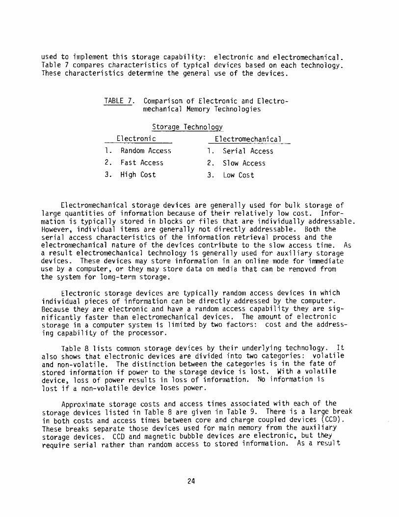
used to implement this storage capability: Table 7 compares characteristics of typical These characteristics determine the general

electronic and electromechanical. devices based on each technology. use of the devices.

TABLE 7. Comparison of Electronic and Electro-mechanical Memory Technologies

Storage Technology Electronic Electromechanical

l . Random Access l . Serial Access 2. Fast Access 2. Slow Access 3. High Cost 3. Low Cost

Electromechanical storage devices are generally used for bulk storage of large quantities of information because of their relatively low cost. Infor­mation is typically stored in blocks or files that are individually addressable. However, individual items are generally not directly addressable. Both the serial access characteristics of the information retrieval process and the electromechanical nature of the devices contribute to the slow access time. As a result electromechanical technology is generally used for auxiliary storage devices. These devices may store information in an online mode for immediate use by a computer, or they may store data on media that can be removed from the system for long-term storage.

Electronic storage devices are typically random access devices in which individual pieces of information can be directly addressed by the computer. Because they are electronic and have a random access capability they are sig­nificantly faster than electromechanical devices. The amount of electronic storage in a computer system is limited by two factors: cost and the address­ing capability of the processor.

Table 8 lists common storage devices by their underlying technology. It also shows that electronic devices are divided into two categories: volatile and non-volatile. The distinction between the categories is in the fate of stored information if power to the storage device is lost. With a volatile device, loss of power results in loss of information. No information is lost if a non-volatile device loses power.

Approximate storage costs and access times associated with each of the storage devices listed in Table 8 are given in Table 9. There is a large break in both costs and access times between core and charge coupled devices (CCD). These breaks separate those devices used for main memory from the auxiliary storage devices. ceo and magnetic bubble devices a:e elect:onic, but they require serial rather than random access to stored 1nformat1on. As a result

24

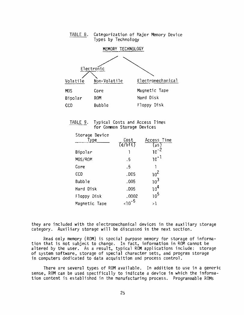
TABLE 8. Categorization of ~lajor Memory Device Types by Technology

MEMORY TECHNOLOGY

Electro~~ 7'\: ~

Volatile Non-Volatile Electromechanical

MOS

Bipolar

ceo

Core ROM

Bubble

Magnetic Tape

Hard Disk

Floppy Disk

TABLE 9. Typical Costs and Access Times for Common Storage Devices

Storage Device Type Cost Access Time

(¢/bit) ( "s) Bipolar 10-2

MOS/ROM .5 10-1

Core .5 1

ceo .005 1 o2

Bubble .005 1 o3

Hard Oi sk .005 1 o4

Floppy Disk .0002 105

Magnetic Tape <10- 5 >l

they are included with the electromechanical devices in the auxiliary storage category. Auxiliary storage will be discussed in the next section.

Read only memory (ROM) is special purpose memory for storage of informa­tion that is not subject to change. In fact, information in ROM cannot be altered by the user. As a result, typical ROM applications include: storage of system software, storage of special character sets, and program storage in computers dedicated to data acquisition and process control.

There are several types of ROM available. In addition to use in a generic sense, ROM can be used specifically to indicate a device in which the informa­tion content is established in the manufacturing process. Programmable ROMs

25

(PROMs) permit users to store their own information using special programming devices. Unless there is provision for alteration of the memory at some later time, once information has been placed in PROM its storage is permanent. Some PROMs are constructed so that they are reusable. The most common of these use ultra-violet light to erase stored information (UV-EPROM). Following erasure, the UV-EPROM may be reprogrammed as if it were new. Both the initial program­ming of PROMs and the reprogramming of EPROMs require special circuits not normally included in applications oriented computer systems.

The total amount of memory devoted to ROM is generally small because of the read only limitation. The majority of a computer•s main memory consists of core and metal oxide and bipolar semiconductor random access devices (MOS and Bipolar RAMs).

Core technology was developed prior to the development of the semiconductor technology. In core memory. an electrical current is used to establish a mag­netic field. The direction of the field depends on the direction of the current. Once established the direction of the field does not change until the current direction is changed, thus core retains information when power is lost. Three factors control the speed of core memory. These are: physical size, access time and time to restore information following a read. When information is read from a core memory location, the information is temporarily lost. To prevent permanent loss, the information must be restored before memory is accessed again. As a result, the true memory speed (cycle time) is determined from a combination of the access time, which is the time to read from core, and the restoration time. There may be an additional delay between access and res-toration to permit the modification of the information prior to restoration.

MOS is a type of field effect transistor. There are several types of MOS including NMOS and CMOS. The differences between the types are related to construction, speed, power consumption and cost. For reference, NMOS memories are faster than core and CMOS memories are faster than NMOS. CMOS memories require less power than NMOS memories. but they are larger and more expensive. We will disregard these differences and consider all MOS memories as a common type.

MOS RAMs are classed as either dynamic or static. Dynamic MOS RAMs require that their contents be periodically refreshed. This imposes a requirement for additional circuitry on the computer system, and in some cases results in memory cycle times that are longer than access times. Static MOS RAMs do not require refreshing; however, they are more expensive. The choice between dynamic and static MOS memories involves a trade-off between the cost of the refresh cir­cuitry and the additional cost of the static MOSs.

Bipolar memories use transition-transistor logic (TTL). They are faster and more costly than MOS memories. The differences in speed and cost are an order of magnitude or more, although the cost difference is being reduced. In addition. bipolar memory requires more power. One of the primary uses of bipolar memory is in a "cache" memory. Cache is a small amount of high speed memory. outside of the main memory, that is used to store frequently used data

26

and instructions. The performance of the computer is significantly improved if a cache memory is used and the computer finds the required information in the cache memory with a high frequency.

Memory cycle times are readily available for computer systems. Table 10 presents reported cycle times for a wide variety of computers. The super computers are represented by CRAY-1, CDC-7600 and Star computers, and the CDC-6600 and Cyber-73 represent mainframe computers. The computers in the next group are microcomputers. The remaining computers are generally classified as minicomputers. If the cycle times for the super computers are ignored, it is apparent that memory cycle times for both micro- and minicomputers approach if not equal the cycle times for mainframes. Further, it is apparent that the ranges for microcomputer and minicomputer cycle times are roughly equivalent. Other items illustrated in the table are, e.g., several memory cycle speeds are frequently available for a single computer model (e.g., PDP-ll/45), 'and differ­ent computer models in the same series may have significantly different memory cycle times (e.g., Texas Instruments 990/10 and 990/12 computers).

TABLE 10. Memory Cycle Times for Typical Computer Systems

Cray-1 CDC 7600 CDC STAR CDC CYBER-73 CDC 6600

Computer

MIPROC 16 Cromemco System 3 Apple II Computer Automation LSI4-90 Data General Micro Nova MP/100

PDP-11/45 (Bipolar) PDP-ll/45 (NOS) PDP-11/45 (Core)

MOOCOMP Classic 7830 Texas Instruments 990/12 Hewlett Packard HP-1000 E Series Harris 500 Data General Eclipse C/150 Sperry-UNIVAC V77-600 Texas Instruments 990/10 CDC Cyber-18 Prime 450

Memory Cycle Time {nanoseconds) -

1. 25 27.5 40.0 100 100

50 200 350 S50 960

300 510 970

125 150 350 400 500 660 570 750 750

Source

McKnight (1979) "

Eckhouse and ~1orris (1979) "

Datapr~ Reports (198DbD

~1emory cycle time tends to limit performance of minicomputers and main­frames, while in microcomputers performance tends to be limited by processor cycle time (Datapro Reports, 1979).

Several features are available that enhance memory reliability. These include parity checking, error checking and correction (ECC), and storage

27

protection and battery backup. When information is stored or transferred with­in computer systems a parity bit is generally added to each byte of informa­tion. This bit is then set to either 1 or 0 to give the information group an even or odd number of 1 1 S. If a computer uses even parity all information groups have an even number of ones. In an odd parity computer all groups have an odd number of 11 S. Parity checking permits the computer to detect single bit errors in stored information. Error checking and correction can detect both 1 and 2 bit errors and can correct single-bit errors. Some form of error identification and correction is becoming important as memories become more dense because the likelihood of random errors is also increasing. Storage protection is needed on multi-user systems to prevent one user from modifying the data or programs of another user. And, battery backup prevents immediate loss of information following a power failure.

AUXILIARY STORAGE

The primary methods of auxiliary data storage are magnetic disks and tapes. Disks are used in online applications where rapid data access is required, while tapes are used for offline storage and data transmittal because of their low cost. It is common to find both disk and tape capabilities in a minicom­puter system. Magnetic drum memories are no longer common.

Disk technology has developed along two lines: hard disks and flexible (floppy) disks. Hard disk systems have higher rotation rates (~3600 rpm) and therefore higher performance than floppy disk systems. The rotation rate of floppy disks is typically of the order of 360 rpm. Hard disk systems were developed first and are common in mini and mainframe computer systems. As low­cost hard disk technology (Winchester) is developing, hard disks are being added to microcomputer systems. Floppy disk systems are common in both minicom­puter and microcomputer systems.

Hard disk systems are sealed units in which the heads ride on a cushion of air just above the disks. Fixed head drives give higher performance than moving head drives, but tend to be more expensive. However, the differences in performance are relatively small. Moving head drives generally provide more storage capacity for a fixed price. The storage capacity of hard disks is greater than lM byte per disk. In small systems it is typically in the 4 to 10M byte range. The disks may be fixed to the drive, or they may be removable in single disk cartridges or multidisk packs. Hard disk access times of 10 to 100 milliseconds are common.

Floppy disk systems provide a low cost option for bulk data storage where hard disk performance and storage capacity are not needed. Typical access times for floppy disk systems are 100-500 milliseconds. Storage capacity depends on disk size and is generally less than 500K bytes per disk. Floppy disks come in two sizes. The larger size is 8 inches in diameter and has a capacity of 240 to 340K bytes per side at n~rmal data density. The smaller floppy disks are 5-l/4 inches in diameter and have capacities of 50 to 90K bytes. These ranges

28

exist because of differences in the number of tracks and the ways in which the disks are sectored. Magnetic disks are divided radially into pie-shaped sec­tors. This permits data to be addressed by sector and track; it also permits data in one location to be changed without affecting data in another location. Systems are available that use both sides of the disk and record data at double density.

Floppy disks are contained in protective covers and are removable, but they are not sealed. As a result, the disks are inexpensive (<$5.00) and are used for archiving or transmittal of data. However, the interchangeability of disks between systems is limited by lack of standardized disk formats.

Magnetic tape technology has also developed along two lines. reel-to-reel technology has been the standard. However, recently cartridge systems have become readily available.

Historically, cassette and

Standard reel-to-reel tape units use l/2 11 wide magnetic tape on 7, 8 l/2 or 10-l/2 inch diameter reels. A 10-l/2 inch reel contains 2400 feet of tape. The data storage capacity of a tape depends on its length and the recording format. At a recording density of 1600 bits per inch (bpi), a 2400 foot tape could contain about 46M bytes of information. In practice, the capacity of the tape is less than the maximum possible because the information is grouped into records and files that are separated by inter-record gaps and file marks.

Tape format includes the number of tracks, the recording method, and the recording density. Both 7 and 9 track tape drives are available. Nine track drives are currently more common. In the 9 track format, 8 tracks are used for data and the other track is used for a parity bit. The standard data densities for 9 track tapes are 800 and 1600 bpi. Seven track systems are most frequently used with computers having a word size that is a multiple of 6 bits. Lower recording densities (200, 556 or 800 bpi) are typical for 7 track tapes.

The most common tape recording methods are NRZI (nonreturn to zero, inverted) and PE (phase-encoded). Both methods utilize a change in magnetic flux to indicate data. In the NRZI method, a change in flux is used to indicate a one and a zero is indicated by not changing flux. In the PE method, both one and zero are indicated by flux reversal; the direction of reveral is used to distinguish between them. The PE method includes timing information on the tape and is less susceptible to tape problems.

The access time to retrieve data from tape depends on the position of the data on the tape and the position of the tape. If the tape is positioned so that the data are near the read head, access times of the order of a second are possible. However, if a significant portion of the tape must be scanned to find the data, access times of several minutes are possible. Tape systems are available with transport speeds between a few inches/second and more than 100 inches per second.

A variety of cassette and cartridge tape systems are available. Some of these units use a Phillips cassette, others use what is called a 3M cartridge, and still others use speci a 1, proprietary cassettes or cartridges. Tt;e primary

29

advan~ages of these tape units are the small cassette and cartridge sizes and relat1vely low system costs. The storage capacities of cassette and cartridge tapes are less than that of a 10-l/2 reel of l/2 inch tape. Capacities approaching 1M byte are claimed for some Phillips cassette systems, and 3M cartridge systems with a capacity of 17M bytes are advertized. Standardization may be a problem if data are to be recorded on one system and read by another.

Punched cards and punched paper tape can be considered to be bulk storage media. However, they are more appropriate for program storage than for data storage, and are more likely to be useful in system development than they are during system operation. The time constraints that exist during an emergency are such that operational program storage on disks or in ROM is more appropriate than storage on cards or paper tape. Thus, the value of punched card and punched paper tape systems should be judged primarily in terms of their utility in the program development.

INPUT/OUTPUT DEVICES

The computational hardware just discussed and the software to be discussed later are important components of an emergency response computer system. How­ever, the most important components in the system may be the input/output (I/O) devices. In this section we will discuss common I/0 devices and identify fea­tures of these devices that can be used to enhance the user/computer information exchange process.

The primary I/0 device for minicomputer systems is a video display terminal (VDT). For our purposes it consists of a cathode-ray tube (CRT) display, video circuitry to drive the display and a keyboard for user input. These components are typically contained in a common enclosure, although some VDT 1 s are available with detachable keyboards. Where user input is not required, information can be presented on a CRT display monitor. In this case the display video circuitry can be located near the CPU.

Video display tenninals are frequently described as "dumb, u 11 Smart" or

intelligent." The distinction is related to the functional capabilities of the terminal. A dumb tenninal does little more than relay infonnation between user and computer. All of the information processing occurs within the computer. A smart terminal generally contains a microprocessor and some memory. This permits the information presented on the display to be stored in local memory and relieves the computer of some display related tasks. It also makes it pos­sible to define special function keys that simplify terminal usage and data input. An intelligent terminal has local data processing and storage capabil­ities that are significantly greater than those in smart terminals. These tenninals are typically capable of stand-alone operation. That is, they are· fully user programmable in a high level language and have sufficient memory to hold useful programs. Many intelligent terminals also include or have provision for control of peripheral devices such as floppy disks and printers.

VDTs can generally be categorized in a second manner dealing with the dis­play capability. The most common and least expensive VDTs are alphanumeric

30

terminals. Graphics terminals are somewhat less common and more expensive, but still readily available. The next few paragraphs describe the uses, character­istics and special features of available terminals.

Alphanumeric VTDs are used to display information in an alphanumeric form. Typical information displayed might include messages about computer status, pro­gram availability and operation, instructions for program execution, input data and program output. Alphanumeric VDTs are commonly used for program development.

The primary display attributes of an alphanumeric VDT are the character set, the number of characters displayed per line and the number of lines on the display. The typical VDT displays 80 characters per line and has a 24 or 25 line display capability. There are VDTs available that use high resolution CRTs and are capable of displaying 132 characters per line and 48 lines. There are also VDTs available with less resolution, and thus less display capability than normal. Most VOTs use some portion or all of the American Standard Code for Information Interchange character set. The lower case letters are the por­tion of the ASCII character set most frequently excluded. Extended character sets that include a limited number of graphics characters are also available.

Special features are included in many VDTs to improve their utility, the clarity of information presentation, and/or reduce the load on the computer. Common features include:

• reverse video • additional display memory/scrolling • blinking fields • cursor control • variable intensity • numeri ca 1 key pad • underlining • special function keys • split screen • integral modem • protected field • printer port

The first four of these features can be used to highlight information contained on the display. Normal display presentation is a light image on a dark back­ground. By reversing the presentation, a character or group of characters can be made to stand out. A similar effect can be obtained by flashing characters on and off, changing the intensity of a portion of the display, or underlining.

The split screen feature gives the programmer additional flexibility. With this feature a single VDT can be treated as a group of smaller di~plays. In an emergency response computer system, one of the smaller displays might be used to list procedures, a second to list atmospheric models available, a third might be used to list model input parameters, and a fourth might be used to summarize model results.

The protected field feature prevents a user from changing the information presented in the field. In emergency response applications this feature may be appropriate from a quality assurance point of view. Through its use, program­mers can permit users to enter or modify selected information while not jeo­pardizing other information needed for program operation.

31

Increased display memory is used in some VDTs to permit the user immedi­ate access to more information than can be displayed at a single time. The displayed information can be changed by moving forward or backward in the memory. This is accomplished by use of a scrolling key. Moving forward in memory causes the text on the screen to rise as new lines are added at the bottom of the display. while moving backward causes the text to, descend.

In an emergency system where manual data input is required, direct cursor control is a useful VDT feature. The VDT cursor is a marker that indicates the position in which the next character will be entered. With direct cursor control, if an error is discovered while entering data, the cursor can be moved to the location of the error and a correction can be made without affect­ing data that were entered after the initial error but prior to its discovery.

Numerical keypads and special function keys facilitate data entry. Num­eric keypads associated with VDTs are based on the standard keypads used for 10 key adding machines. In some cases the standard 10 key numeric pad is augmented with keys for cursor control and screen editing. Special function keys may include editing features. They may also be used to recall lists of available programs and initiate program execution. In the latter case the use of a special function key may significantly reduce the number of key strokes required and thus decrease the chance for user error in an emergency situation.

The remaining special features in the list are an integral modem and a printer port. Integral modems are found on a few VDTs. The primary advantage of an integral modem is consolidation of devices within a single cabinet. In the case where the VDT is connected directly to a computer without use of a modem, the integral modem would facilitate reconfiguration of the system in case of computer failure. The VDT printer port may be associated with a key that permits the terminal user to copy the display to a printer, assuming a printer is attached. This feature might be particularly useful if information is relayed from a terminal in one location to a terminal in another.

Graphics terminals have enhanced display capabilities. In addition to dis­playing a set of predefined characters, they can display shapes defined under program control during program execution. As a result, they are more versa­tile than alphanumeric terminals. Characteristics of graphics terminals that are worthy of consideration include: resolution, display tape, color and special features.

The basic picture element on a graphics display is called a pixel. If the display has a large number of these elements in the horizontal and vertical, the display has high resolution. A standard TV Display consists of 525 hori­zontal lines and has a width to height ratio of 4 to 3. Assuming that TV pixels are square and have sides equal to the vertical width of a line, the resolution of a TV set would be described as 700 x 525 pixels. This is relative high resolution.

As resolution is reduced by increasing pixel on a checkered rather than continuous appearance.

32

size, graphics displays take This effect is clearly

illustrated by the appearance of diagonal lines. In high resolution a diagonal line appears as a continuous straight line, while in low resolution it appears as a series of steps. The lowest resolution acceptable for emergency response graphics terminals should be determined by model accuracy and user reaction. It is likely that adverse user reaction to the discrete blocks on a display will ultimately limit resolution.

Two techniques are used to control the electron beam in graphics terminals. The raster scan technique is the same as used in television sets. The electron beam starts at the top of the CRT and moves horizontally from left-to-right. At the completion of each horizontal scan, the beam is lowered and another left-to-right scan is started. This continues until the bottom of the display is reached, then the entire process is repeated. Thus the electron beam scans the entire CRT. In a vector graphics terminal, the electron beam is not con­strained to move horizontally. It can move directly from one point on the screen to any other point. As a result it is not necessary to scan the entire tube. Vector graphics terminals provide higher resolution and are more effi­cient for line drawing; raster scan terminals are less expensive and more efficient where areas are to be shaded. There are graphics terminals that have both raster and vector scan capabilities.

Graphics terminals are available with displays ranging from black and white through multiple shades of gray to color. Black and white graphics terminals are least expensive because they require the least circuitry and dis­play memory. They also have the least ability to communicate information.

Terminals with multiple shades of gray require essentially the same cir­cuitry and display memory as color terminals, but they use less expensive CRTs. The use of several gray shades permits display of more information than can be displayed on black and white terminals because lighter shades of gray can be used to identify regions of interest such as high population areas without the use of lines. Lines can be used for plume positions, roads, etc. The informa­ton content of these displays is limited by the number of shades of gray and line types that can readily be distinguished by the user.

The number of colors available in color displays systems typically ranges from 4 to 4096. Many systems have a large number of colors available, but require the programmer to restrict the number used at any one time to a rela­tively small number. Some of these systems permit separate selection of fore­ground and background colors. Other special features found on graphics termi­nals include: scrolling and zooming, color change capabilities and routines to fill areas.

The memory and computational requirements of graphics terminals are suf­ficiently large that they should be separated from the host computer. As a result, many graphics terminals are highly intelligent. In a typical applica­tion, the host computer would do model computations and the terminal would prepare the display presentation. If the host computer were required to use its memory and CPU for graphics purposes, its computational capacity and efficiency would be significantly reduced.

33

Several devices are frequently used for data input with graphics terminals. These devices include graphics tablets, light pens, and touch screens. Graphics tablets are particularly useful for entering information such as geographic features, roads, population centers and political boundaries. With a tablet this information can be transferred directly from maps; conversion to digital values occurs automatically. Light pens and touch screens permit the computer user to choose among items presented by the computer without the use of a keyboard. The items might include program or display options.

Video display terminals provide an excellent means of communication between user and computer, however they have some shortcomings. These are primarily related to the provision of permanent records. Records are essential if the sequence of events is to be faithfully reconstructed during post acci­dent evaluation. The devices available that might be used in keeping these records include printers, hard copy units and plotters.

Printers provide a primary means of making a permanent record of informa­tion presented on alphanumeric VDTs. Some also have limited graphics capabil­ities. Printers can be generally classified as line or character printers. Line printers print an entire line of text at one time. They are high speed devices that are used where high volume output is required, and they are rela­tively expensive. Character printers print a single letter at a time and are therefore relatively slow. Print rates for character printers are typically in the 30 to 300 character per second range. The speed of character printers should generally be adequate for emergency response systems.

Printer technology includes both impact and nonimpact devices. The non­impact printers tend to be faster. This type includes thermal, electrostatic and ink jet printers. Impact devices include dot matrix and daisy wheel printers. Thermal, electrostatic and dot matrix printers tend to be less expensive than ink jet and daisy-wheel printers, and should provide acceptable quality output. Thermal and electrostatic printers require specially treated paper.

Ink jet and dot matrix printers have the most versatility in presenting graphical output. They can produce varying shades of gray by changing their dot densities. Some ink jet printers are also capable of producing color graphics. The graphics capability of the other printer types is generally limited to varying shades of gray caused by selecting different letters and overprinting. Printer graphics greated by character selection and overprinting is not equivalent to the display on a graphics VDT.

There are hard copy devices that are capable of reproducing the display of a graphics terminal. In addition to ink jet and dot matrix devices, there are laser xerographic and photographic devices. Factors to be considered in selecting a hard copy unit are speed, resolution and cost. High speed, high resolution devices are relatively expensive, although the cost of indivdual copies made with the devices may be relatively inexpensive (a few cents per copy}. Ink jet printers, laser xerographic and photographic copiers may be capable of color reproduction.

34

The final devices that might be considered for production of permanent records are plotters. Plotters are relatively inexpensive and are available from a number of vendors. Special features available on some plotters include multicolor plotting and plotting on continuous paper rolls.

COMMUNICATIONS

The communicatons subsystem provides for an orderly flow of data and information within the computer system. Primarily we are concerned with the transmission of data and information from data acquisition systems to computers and between computers and terminals. The first of these concerns is a short range communicatons problem and the second may be either a short or long range problem. Peripherally we are also concerned with the transmission of data from sensors to data acquistion systems and within computers. These are generally short range problems and are accomplished by direct hardwired connections. As a result, we will not consider them further.

The conceptual division between short and long range communications is based on both economic and physical considerations. The relative costs of com­munications hardware and the transmission medium change as the transmission distance increases. Similarly, the distortion and attenuation of the trans­mitted signal increase with increasing distance. In both cases the rates and magnitudes of the changes depend to a large extent on the transmission techni­que being used. There is no sharp division between short and long range com­munications, however an approximate dividing point might be about 10 miles.

The orderly flow of information requires that rules and procedures for data transmission be established and followed. These rules and procedures are called communications protocol. Weitzman (1980) divides protocol into four levels, each level building on lower levels. As the level becomes higher, the protocol becomes more user oriented.

The lowest protocol level describes physical connections between the com­puter and the communications subsystem. This level may refer to standard elec­trical interfaces such as RS-232C or IEEE-488. The RS-232C interface is com­monly used with serial data transmission. (Most communications between devices more than a few feet apart is accomplished using serial transmission). More recent interface standards (RS-422 and 423) have same advantages over RS-232C for use with integrated circuits. However their use is not as common as is the use of RS-232C. Use of the IEEE-488 interface standard is common in parallel data transmission, such as between terminals and printers.

The second protocol level involves the communications link. It includes items such as information coding, character framing, error handling and line utilization. Information coding involves selection of a character set for use in data transmission. Common character sets include ASCII and EBCDIC. The ASCII character set is described by Lines (1980) and Parsons (1980). Lines also describes the EBCDIC and several less commonly used sets.

35

Character framing deals with transmission details such as synchronization between sending and receiving stations, and with the addition of bits to the data to control transmission. Asynchronous data transmission is simpler than synchronous tramsmission. It involves sending information one character at a time. Prior to transmission a start bit and one or two stop bits are added to each character (seven bits are used to identify the character and 1 bit is used for parity). In synchronous transmission, characters are transmitted as a unit. Synchronous data transmission is more expensive, but permits the use of more sophisticated error handling techniques.

Error handling involves both error identification and error correction procedures. Common error detection techniques involve parity and cyclic redun­dancy checks {CRC). Parity checks can be done on a character by character basis or on a message basis {longitudinal redundancy check). In either case only odd numbers of errors are detected, e.g., a single error, three errors, etc. CRC is a more sophisticated procedure that can detect errors not detect­able by parity checks. If an error is detected in a data transmission, the most common recovery procedure is for the receiving station to request retrans­mission of the character or message. Techniques exist that permit receiving stations to locate and correct errors; however, they are not commonly used because of lower reliability and an excessive communications burden related to additional information needed for error detection and correction.

One of the characteristics of the line utilization portion of a protocol covers the transmission modes. The transmission modes are simplex, half-duplex and full duplex. A simplex transmission mode allows transmission in only one direction. In a meteorological system it might be used for trans­mission of data from sensors to a data acquisition system or from a data acqui­sition system to a computer. Both half- and full-duplex modes permit two-way transmission. The difference between the two modes is in sequencing. In the full-duplex mode, transmission can take place simultaneously in both directions. In the half-duplex mode information can only be transmitted in one direction at a time. Full-duplex transmission generally requires four wires (or the equiva­lent) between stations.

The highest level protocols are generally written for specific groups of computers and users. Level three covers message routing between end points, and level 4 establishes the languages used and system services such as file handling, record transmission and file security.

Weitzman {1980) contains a comprehensive discussion of communications pro­tocols. His Appendix A contains a synopsis of common protocols including: BISYNC, DDCMP, ADCCP, SDLC, HDLC, X.25, CDCCP and BDLC. In addition, it con­tains a summary of the hardware implementations of various protocols.

Although computers primarily use digital circuits, data transmission over distances of more than a few feet is more easily accomplished with analog sig­nals. Thus most short and long range communications systems rely on devices called modems to convert digital signals to an analog representation for trans­mission and to convert analog signals back to digital form at the receiver.

36

They were first used to transmit data over voice grade telephone lines, and are now used in a wide range of applications. The word modem is derived from modulation-demodulation, which describes its function. The transmitting modem sends it signals by varying one or more of the following wave characteristics; phase, amplitude or frequency. The major types of modulation are frequency shift keying (FSK), amplitude modulation (AM), and phase modulation (PM). Quadrative amplitude modulation (QAM) varies both amplitude and phase to achieve higher data rates than the other methods.

Data transmission rates are given in bit rate. Bit rate refers to the actual number of data units transferred per unit of time. Baud rate refers to the number of electrical signals transferred per unit of time; at low speeds the two rates are the same. However, to obtain high speeds, two or three data bits may be packed in one electrical signal to give a bit rate two or three times higher than the baud rate. The user is primarily concerned with bit rate. Modems operate over a wide range of transmission speeds. These speeds can be divided into five basic groups:

1 ow speed medium speed high speed wide band fiber optic speed

up to 600 bits/sec 1.2 to 2.4K bits/sec 3.6K to 9.6K bits/sec up to 19.2K bits/sec and higher up to 56K bits/sec

If a large amount of data is to be transmitted, the data transmission rate becomes an important consideration. Consider the transmission of data from a full VDT display (25 lines x 80 characters/line). This requires the transmis­sion of 20,000 bits, assuming asynchronous transmission of ASCII code with one start and one stop bit. At 300 bits/second (~300 baud) it would take ~67 sec­onds. At 1200 bits/second it would take 17 seconds, and at 9600 bits/second just over 2 seconds. In terms related directly to emergency response, trans­mission of the information described in Appendix B of Revision 1 to Regulatory Guide 1.23 would require ~99 seconds at 300 bits/second, 25 seconds at 1200 bits/ second or 3.1 seconds at 9600 bits/second.

In selecting a modem, it is necessary to consider the protocol being used and the transmission distance. Short transmission distances and synchronous protocols are most compatable with high speed data transmission. The use of long distance telephone lines limits data transmission rates. On these lines, transmission rates of 300 to 1200 bitsjsecond are realistic. If leased lines are used, and if circuitry is added to compensate for line distortion and signal attenution, a transmission rate of 9600 bits/second is realistic.

Many options are available on off-the-shelf modems. Among the more common options are: selectable transmission rates, transmission line equalization, direct connection to telephone lines, and automatic dial and answer capabi 1 i ties.

With in the current context, s hart range data transmission might inc 1 ude communication from the meteorological sensors to the plant and local

37

communications between the Control Room, Technical Support Center and the Emergency Operations Facility. Short range transmission media must be very reliable and either error-free or contain an accurate error checking provision. Speed of transmission is not a limiting criterion since almost all transmission media are capable of handling the required communications in real time. Pri­vate wire, UHF radio telemetry, and fiber optics are the most likely means of data transmission for these applications. Microwave telemetry discussed under long range communication is also reasonable. Satellite transmission is not realistic because of low availablity of channels and the high cost of receiving stations.

Private wire is highly reliable and inexpensive for transmission over short distances. Transmission is digital with simplex, half duplex, and full duplex modes possible at data rates from 1M to 2M bits/second. Line drivers and receivers, modem eliminators, or limited distance modems can be utilized. Errors in the line may occur due to electrical or magnetic interference; how­ever, error checking devices are common in the interface units. Cost increases significantly with distance, especially if the distance is such that the wire must be installed aerially, or in underground conduits for protection. Availability is high; the line can be purchased and installed quickly for short distance applications.

Meteorological data may be transmitted in the 100-500 MHz radio-frequency band. But, because ultra-high-frequency signals must be sent line-of-sight, repeater statons may be needed in complex terrain. Transmission is reliable and circuitry usually contains error checking devices which retransmit faulty data. Transmitters and receivers can be purchased off-the-shelf.

Fiber optics is a relatively new technology in which data are transmitted digitally by light pulses through a thin glass fiber. Two of the main advan­tages of fiber optics are high data rates and no electrical or magnetic noise. Fiber optic lines also offer a high degree of security. They can only be tapped by breaking the line and setting up highly complex transmission equip­ment at the break. If installed properly, fiber optics has a high degree of reliability. However, installation and maintenance procedures are highly precise. Fiber optic tranmission is not cost effective for low usage or low data rates.

Long-range data transmission refers to transmission to offsite terminals. The most common means of long-range data transmission are privately-leased and public-switched telephone lines. Telephone companies also offer special ser­vices for data transmission such as Wideband Analog and Dataphone Digital Ser­vice. Other means of transmission include microwaves, satellites, and very­high-frequency radio.

For long distance data transmission, the public-switched network has many advantages. It is relatively inexpensive, the user can get a variety of data rates and can communicate with any of the locations served by the network, and lines are readily available. Costs, which vary depending on transmission speed required, range from as little as $25 per month for an 800 baud line to $140

38

per month for a 4800 baud line. Lines are usually two-wire and thus require either rental of two lines or use of a frequency splitting modem for full duplex transmission.

Although telephone companies aim for no more than 15 errors in 15 minutes, data transmission on public-switched networks is subject to noise from electri­cal interference, relay switching, and line signal distortion. Many communi­cations systems contain error checking devices which automatically trigger retransmission of faulty data. However, retransmission slows down total data throughput. Telephone lines are vulnerable to storms and other adverse weather conditions. In addition, accessing the line may be difficult at times, espe­cially in emergency situations when local switches are overloaded.

Leased private telephone lines can be electronically conditioned to reduce signal distortion and attenuation and thereby give a better quality transmis­sion and higher data rates than public-switched lines. Achievable data rates may be as high as 9600 bit/second. Synchronous and asynchronous transmission are available, and leased lines may be four-wire to allow fully duplex trans­mission. The cost of leased lines varies with distance, type of conditioning, and speed. A typical cost for a 9600 bit/second line is $230 per month.

Bell and General Telephone provide special services for transmitting data. Wideband analog services, such as Bell Telephone 1 S TELPAKC, TELPAKD and Series 8000, are collections of voice grade channels that can accomodate data transmission at up to 230.4K bit/second. Bell 1 s Dataphone Digital service is available in many of its 96 FCC-approved metropolitan areas. This service can send data at rates of up to 1.544M bit/second with fewer errors and lower cost than conventional analog facilities. The system is guaranteed to have 99.5% error-free seconds and to be available 99.96% of the time. General Telephone 1 S 56000 windband analog services can accommodate a data rate of up to 56K bits/second.

Microwave transmission of data can occur at high data rates and is rela­tively reliable because there are no long distance lines to fail. Error fail-ure rates of as low as 1 in 108 have been measured. Microwave transmission is line-of-sight, thus the expense of repeater stations (~$70,000) about every 30 miles is a significant drawback for long-range transmission unless existing facilities can be used. Other potential sources of problems in microwave com­munication are temporary misalignments of antennae caused by high winds and reflections from aircraft.

Very-high frequency {VHF) radio can transfer data over long distances at a low cost. However, the error rate with this type of transmission can be as high as one percent. In addition, reliability is poor and authorized frequen­cies, which must be obtained from the FCC, are not readily available. VHF radio, although suitable for voice transmission, is not acceptable for trans­mitting data in emergency situations.

Communication satellites can be used as relay stations in long-range data transmission systems. Data transmission rates in these systems are 4K to 1.5M

39

bits/second and the error rates are low (~lo- 8 ). channels, themselves, are highly reliable because vulnerable ground lines.

In addition they do not

the trans~ission depend on long,

Satellite communications channels are commercially available from several sources. There are also open channels on the NOAA operated Geostationary Earth Satellites (GOES). There currently are 3 GOES satellites, each having 266 transmission channels. The use of GOES is limited to the transmission of environmental data and is controlled by the National Environmental Satellite System (NESS), a section of NOAA. It is not available- for use where adequate service can be provided by telephone lines. Priorities tor assignment and use of GOES transmission channels, in order, are:

• NOAA • those who provide data to NOAA • those who provide data to other Federal Government agencies • those who provide data to State and local Governments.

Further, data collection and transmission equipment used in conjunction with GOES must meet NOAA specifications, and NOAA and other government agencies must have free use of the data.

Data collection and transmission systems meeting NOAA specifications are available off-the-shelf for about $5,000. Other costs associated with use of the GOES include the rental of the channel and the lease of land transmission lines where needed. Transmitter stations are relatively inexpensive, but receivers are quite expensive (~$70,000). At these prices satellite transmis­sion is not economical for distances of less than 800 miles. Another disad­vantage of satellite transmission is the propagation delay due to the total dis­tance the signal must travel. With various error checking protocols this delay can reach 0.25 to 0.50 seconds per transmitted group.

The advantages and disadvantages of various data transmission techniques are summarized in Table 11.

If the computational load in a computer system is divided among two or more components, the system is a computer network. Computer networks are described by: the functional compatability of the computers, the method by which the computers are connected, and the functional relationship between the computers. If the computers are functionally compatable (the same architecture), the net­work is called homogeneous, otherwise it is called heterogeneous. Similarly, if the computers in a network share main memory, the network is called closely coupled; if not, the network is called loosely coupled. Finally, if one of the computers in a network controls the others, there is a master-slave relation­ship between computers, while if all the computers are equal there is a master­master relationship. Weitzman (1980) claims that almost all micro- or minicom­puters can be combined in loosely-connected, heterogeneous networks on either master-slave or master-master bases. Weitzman (1980) provides the following

40

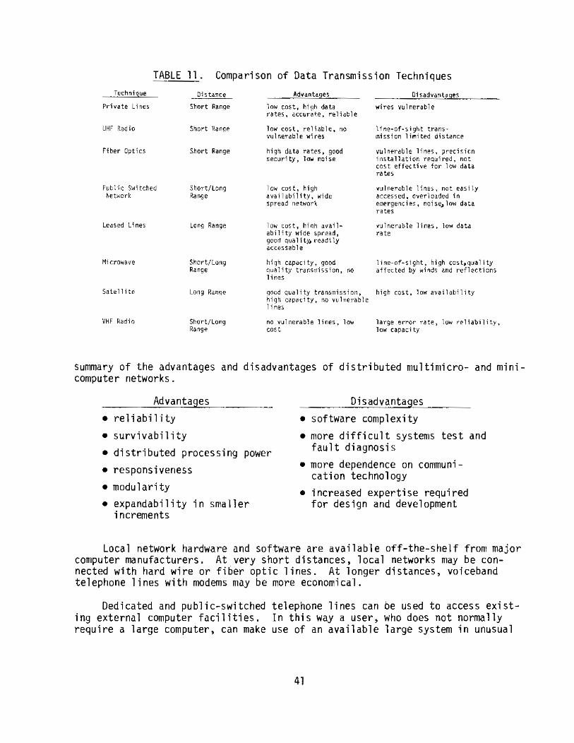
TABLE 11. Comparison of Data Transmission Techniques Technique

Private Lines

UHF Radio

Fiber Optics

Public S·o'litched ~et~·ork

Leased Lines

M1crowave

Satellite

VHF Radio

Distance

Short Ranqe

Short Ran~e

Short Range

Short/Long Range

Long Range

Short/Long Range

Long Ranqe

Short/Long Range

Advantages

low cost, hioh data rates, accurilte, reliable

low cost, reliable, no vulnerable wires

high data rates, good security, low noise

low cost, high availability, wide srread network

low cost, hiqh avail­ability wide spread, good qual it» readily accessable

hiqh capacity, good quality transmission, no lines

ooad quality transmission, high caoacity, no vulnerable lines

no vulnerable lines, low cost

Disadvantages

wires vulnerable

line-of-sight trans­mission limited distance

vulnerable lines, precisicn installation required, not cost effective for low data rates

vul~erable lines, not easily accessed, overloaded in emergencies, noise~ low data rates

vulnerable lines, low data rate

line-of-sight, high cost.quality affected by winds and reflections

high cost, low av~ilability

large error rate, low reliability, low capacity

summary of the advantages and disadvantages of distributed multimicro- and mini­computer networks.

Advantages

• reliability

• survivability

• distributed processing power

• responsiveness

• modularity

• expandability in smaller increments

Disadvantages • software complexity • more difficult systems test and

fault diagnosis • more dependence on communi­

cation technology • increased expertise required

for design and development

Local network hardware and software are available off-the-shelf from major computer manufacturers. At very short distances, local networks may be con­nected with hard wire or fiber optic lines. At longer distances, voiceband telephone lines with modems may be more economical.

Dedicated and public-switched telephone lines can be used to access exist­ing external computer facilities. In this way a user, who does not normally require a large computer, can make use of an available large system in unusual

41

circumstances without undue expense. When intertied with a larger system, the user 1

S own system acts as a local terminal in a widely distributed, loosely coupled network.

OPERATING SYSTEMS AND PROGRAMMING LANGUAGES

In practice it is not necessary for the applications programmer to be intimately familiar with the details of the internal structure of the computer and memory. He can program in a familiar language such as FORTRAN, submit the program to the computer and await the results. This is because of the exis­tence of a series of systems programs within the computer. The operating sys­tem is a major portion of the software that provides the interface between the user and the hardware. It is generally transparent to the user, but without the operating system programming would be much more difficult. Lines (1980) claims that it would be 11 inconceivable 11 for a minicomputer system to exist with­out one, and indicates that reasonably sophisticated operating systems are avail­able for microcomputers.

The basic functions of an operating system are to provide:

• Task Management (scheduling) • Resource Management (memory allocation) • Data Management (control of input/output and communications} • Utility Software (editors, etc.}

While providing these basic services, individual operating systems have been tailored to specific applications such as batch and time-sharing computations, real time control of external functions, data base management and communica­tions. It may be inferred from NUREG-0654, and 0696 that a multi-user, time sharing capability is required for an adequate emergency response computer system.

Lines (1980} describes several approaches followed in multi-user operating systems. The most common system is a closed conversational system in which the users are limited to specific languages and resources. Typically these sys­tems can accommodate 8 to 64 users programming in a high level language such as FORTRAN. Further, the number of users is generally limited by available memory rather than by computer power.

Computer programming languages vary in sophistication from the binary, octal or hexadecimal instruction sets used by the processor to high level languages such as BASIC, FORTRAN, PASCAL and ADA. Most programming is done in either a high level language or in a low level assembly language. Advantages of each level are listed in Table 12.

BASIC and FORTRAN are familiar to most scientific prograrroners. Programs writ­ten in a standard version of either language can be adapted to most computers having the language capability, providing the system has adequate resources. PASCAL is a language that is rapidly gaining acceptance with scientific

42

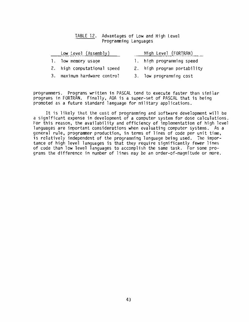
1 .

2. 3.

TABLE 12. Advantages of Low and High Level Programming Languages

Low Level (Assembll) High Level (FORTRAN)

low memory usage 1 . high programming speed high computational speed 2. high program portability maximum hardware control 3. low programming cost

programmers. Programs written in PASCAL tend to execute faster than similar programs in FORTRAN. Finally, ADA is a super-set of PASCAL that is being promoted as a future standard language for military applications.

It is likely that the cost of progran~ing and software development will be a significant expense in development of a computer system for dose calculations. For this reason, the availability and efficiency of implementation of high level languages are important considerations when evaluating computer systems. As a general rule, programmer production, in terms of lines of code per unit time, is relatively independent of the programming language being used. The impor­tance of high level languages is that they require significantly fewer lines of code than low level languages to accomplish the same task. For some pro­grams the difference in number of lines may be an order-of-magnitude or more.

43

COMPUTER SYSTEM RELIABILITY

Reliability is an important consideration in selecting and evaluating com­puter systems for emergency response applications. In this section we define terms related to reliability, discuss the reliability of computer system com­ponents, and demonstrate the estimation of system reliability. No atte~pt i~ made to evaluate a specific computer system because of the number and d1vers1ty of the factors affecting the reliability of specific systems. Some of the factors are under the control of the manufacturer and others are under the control of the user. Table 13 lists important factors in each category.

TABLE 13. Factors Contributing to Computer System Reliability

Manufacturer User

• Computer design/component • Computer environment quality • Usage

• Quality assurance/testing • Maintenance policies • Modularity of construction • Spares inventory • Diagnostic features • Maintenance support • Documentation

We also briefly discuss the reliability of the computer system-human informa­tion exchange process.

Typical reliability analyses are based on four premises:

1. A faulty part can fail only once before being replaced.

2. The variation of failure rate with time follows a U-shaped curve (Fig­ure 2).

3. The probability of failure-free operation for a fixed period during time represented by the bottom of the U-shaped curve has an exponential distribution.

4. In the same part of the curve, the expected number of failures in a given period of time has a Poisson distribution.

Longbottom (1980) suggests that these premises may not be correct when computer system reliability is considered. He cites problems in the definition of fail­ures and in the failure rate curve.

45

DEFINITIONS

' \ \ \ COMPUTER

\( ' ',

NORMAL PRODUCT ·- ,,, ,........ ,.... -.1 '-J '" ' ...... ---

TIME----------+-

FIGURE 2. Failure Rate Variation in Time

Many computer system failures are intermittent and require no more correc­tive action than restarting the system. As a result, failure rate estimates depend on the individual reporting the rate. User reported failure rates are higher than rates reported by servicemen, which are higher than those reported by manufacturers. To avoid confusion, Longbottom establishes categories of com­puter system interruptions. An incident is defined as a computer system inter­ruption as seen by the user and may be the result of a complete or intermittent failure of some system component. Following an incident, a system restart may be attempted, or call may be made to obtain maintenance assistance. Mainten­ance assistance is referred to as an investigation. Actions taken during an investigation may include repair or replacement of components, reconfiguration of the system to operate without a faulty component, or restarting without mak­ing any changes. Maintainability is related to the average number of incidents or investigations required to correct the cause of a series of related faults. Because of the intermittent nature of failures, that average is likely to exceed one. Table 14 gives criteria for determining qualitative maintainability ratings.

Longbottom shows data to indicate that computer failure rates (whatever definition) are not adequately described by the standard curve. The burnin period (decreasing failure rate with time on the left of Figure 2) for compu­ters is much longer than it is for normal equipment. It may extend for as long as 10 to 12 thousand hours of operating time for new computer system designs, and can cover a thousand hours or more for new installations of established systems. In addition, Longbottom questions whether a constant failure rate is ever established. Periodic changes in operating systems, software, and utili­zation along with maintenance errors tend to reduce the chances of establishing

46

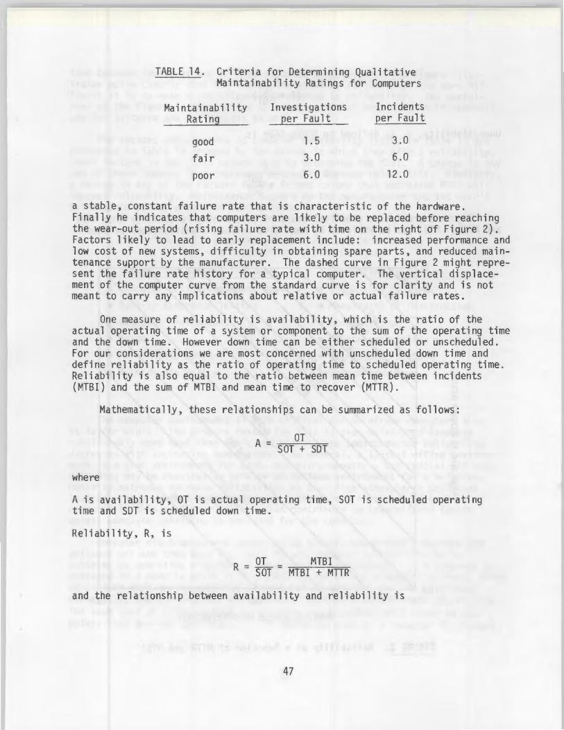
TABLE 14. Criteria for Determining Qualitative Maintainability Ratings for Computers

Mai ntai nabi 1 ity Investigations Incidents Rating per Fault per Fault

good 1.5 3.0

fair 3.0 6.0

poor 6.0 12.0

a stable, constant failure rate that is characteristic of the hardware. Finally he indicates that computers are likely to be replaced before reaching the wear-out period (rising failure rate with time on the right of Figure 2). Factors likely to lead to early replacement include: increased performance and low cost of new systems, difficulty in obtaining spare parts, and reduced main­tenance support by the manufacturer. The dashed curve in Figure 2 might repre­sent the failure rate history for a typical computer. The vertical displace­ment of the computer curve from the standard curve is for clarity and is not meant to carry any implications about relative or actual failure rates.

One measure of reliability is availability, which is the ratio of the actual operating time of a system or component to the sum of the operating time and the down time. However down time can be either scheduled or unscheduled. For our considerations we are most concerned with unscheduled down time and define reliability as the ratio of operating time to scheduled operating time. Reliability is also equal to the ratio between mean time between incidents (MTBI) and the sum of MTBI and mean time to recover (MTTR).

Mathematically, these relationships can be summarized as follows:

OT A = SOT + SOT

where

A is availability, OT is actual operating time, SOT is scheduled operating time and SOT is scheduled down time.

Reliability, R, is

OT MTBI R = SOT = MTBI + MTIR

and the relationship between availability and reliability is

47

from one pattern to the other, the reliability of the system will decrease until weak components adversely affected by the change are eliminated.

Another usage factor that affects computer reliability is computer system loading. Given two computer systems with inherently equal reliability operated with different loads, the system with the lightest load is likely to appear to be the most reliable. This is particularly the case when reliability is deter­mined from MTBI and MTTR.

Vendor maintenance support and user maintenance policy contribute to reliability to the extent that they enhance the identification and correction of existing or potential faults during scheduled maintenance periods. Many mini- and microcomputer manufacturers are incorporating features in their designs that are intended to reduce the time required to identify failures and complete the necessary corrective action. Self-diagnostic routines, similar to those found on mainframe computers are appearing on small systems. These features identify and flag high temperatures, processor parity errors and abnormal power status among other things. Some computers also duplicate criti­cal circuits to increase reliability.

Modular construction tends to decrease the MTTR. The number of circuit boards included in mini- and microcomputers is small enough that it may be pos­sible for the user or the vendor's local representative to carry a full set of spare modules. Then, in event of a failure, it is only necessary to identify and replace the faulty module. Identification of the faulty component and repair of the module can be completed after the system is returned to opera­tion. Good documentation speeds the identification of faulty modules and components.

The effect of user maintenance policy, vendor maintenance support and spare parts inventory on MTTR should be reasonably evident with a brief examination of the time components in MTTR. These components are:

• The time required to restart the computer, load system routines, and resume processing user programs.

• The time required to locate and inform maintenance personnel of a problem.

• The time spent waiting for maintenance personnel to arrive at the computer.

• The time required to identify the problem and correct it.

• The time required for the vendor's maintenance support personnel to arrive if their assistance is needed.

• The time spent waiting for replacement parts if not available locally.

Computation of an MTTR requires that each of these components be included in a realistic manner. Proper weighting of the times depends to a large extent on the user's maintenance policy. For example, it may be standard practice to

50

attempt a restart prior to calling for assistance, and several restarts may be attempted prior to system recovery. Further, it is obvious that the location of the lowest level of maintenance assistance is an extremely important con­sideration. MTTRs will be significantly lower with an onsite maintenance capability than they will be without one. It is conceivable that waiting times could be the dominant components of MTTR. As such, they could be the most fertile areas in which to bring about a significant improvement in computer system reliability.

PROCESSORS

Longbottom (1980) provides generic estimates of failure rates (incidents/ 1000 operating hours) for mini- and mainframe processors as a function of pro­cessor speed. These estimates are shown in Figure 4 along with estimates of processor speeds for representative processors (from Table 6). The curves are for high quality computer systems with good maintainability, operating in good environments. The failure rate should be increased if any of these assumptions does not hold. Adjustment factors suggested by Longbottom are given in Table 16. Each adjustment factor should be applied independently. Thus, it would be possible to increase the failure rate by a total factor of 80. In that case, the failure rate scale on Figure 4 would cover the range 8 to 8000 incidents per thousand operating hours. A further increase of failure rate by a factor of 2 to 3 for the first year of a computer design is suggested by Longbottom. A set of adjustment factors is also given to account for differ­ences in computer usage. These range from 1/4 for very low usage to 2 for high usage. No correction factor is needed for moderate usage.

It appears from Figure 4 that reliability decreases with increasing pro­cessor speed. However, if a fixed computational task is considered, the opposite is found to be true. Figure 5 shows estimates of the number of instructions executed per incident as a function of processor speed. They are derived directly from the curves in Figure 4. Figure 5 also shows a compari­son of the number of instructions executed per incident for typical mini, mainframe, and super computers. It provides an indication that typical mini­computer reliability is approximately the same as the reliability of larger computers. The differences may or may not be significant.

A further comparison of reliability of mini- and mainframe computers is contained in Table 17. The ratings shown are based on user satisfaction rat­ings on a scale of 1 to 4, with 1 being poor and 4 being excellent. The rat­ings were obtained in a Oatapro Reports (1980i) survey of 15,000 computer users. The only differences shown are the small differences in maintenance responsiveness and technical support in trouble shooting. They are not large enough to be of practical importance.

51

0 z 0 u u.J V'l

0::

~ V'l

~ 10

1-u ::::> 0:: 1-V'l z

~ ::i == 0 u.J u.J Q..

1.0 V)

0:: 0 V'l V'l u.J

g 0:: Q..

0. 1

CRAY-1+ FAST

CDC 7600+

AP-19<l

Ml PROC-16•

} LARGE MAIN FRAttES

VAX -11, MODC OMP, UNIVAC 1108 PDP-10

ll6 BIT MINI AND MICRO

+ SUPER COMPUTER PROCESSO "MICROCOMPUTER

SLOW

0. 1 1 10

FAILURE RAlE !INCIDENTS per 1000 HOURS OPERATING TIME)

FIGURE 4. Processor Failure Rates as a Function of Processor Speed

52

100

MEMORY

TABLE 17. User Ratings of Reliability Factors for Mini­and Mai nframe Computers

Minicomputers and Small Business Mainframe

Com~uters Comeuters

CPU Reliability 3.3 3.3 Maintenance Responsiveness 3.0 3.1 Maintenance Effectiveness 2.9 2.9 Technical Support in

Trouble Shooting 2.6 2.7 Documentation 2.5 2.5

Estimates of failure rates for main memory are shown in Figure 6. The c~rves are taken from the work of Longbottom; memory cycle times for representa­tlve computers taken from Table 10 have been included in the figure. The strik­ing feature evident is the significant improvement in memory failure rate achieved by incorporation of error correction. As in the case of Figure 4, it may be necessary to adjust the failure rate to account for quality, maintain­ability or environment. The adjustment factors in Table 16 are appropriate for main memories.

PERIPHERALS

Table 18 summarizes Longbottom's estimates of failure rates for common peripheral devices based on medium utilization in a good environment. He sug­gests incident rate adjustment factors of 0.25 and 0.50 for very low and low utilization, respectively. It is unlikely that emergency response system per­pheral utilization could be described as moderate, an adjustment for lower utilization should be appropriate. Adjustments for quality, maintainability and operating environment can be made using the factors in Table 16, if war­ranted. Typical investigation times per incident are also listed in Table 18. These times do not include time spent waiting for assistance or for delivery of spare parts.

Manufacturers of floppy disk systems are claiming a mean time between fail­of about 8000 hours, which corresponds to a failure rate of 0.12 per 1000 hours. If we inflate this figure by an order of magnitude to account for the differ­ence between a manufacturer's failure rate and a user's incident rate, the incident rate for floppy disks is about the same as for hard disks.

54

Vl 0 z 0 L) LLJ Vl 0 ~ L)

:E

~ 1-LLJ -1

~ L)

>-~ 0 :E LLJ :E

100

10-1

1-Vl

+SUPER COMPUTER

•MICRO COMPUTER

L)

:E ~

POP-11/45 CORE---..>-CDC CYBER-18--+-

0

Tl990/10, UNIVAC V77--+-

PO P-11145 MOS ---..

POP -11145 B I POLAR---..

•c ROMEMCO -+­TI990/12 -+­

MOOCOMP CLASSIC 7830 ~ CDC 6600-

•MI PROC 16 ___..., :E < ~

~DC 7600~~ -1

~

~ +CRAY-1--+-10 -2 .__ _ _.___.__._--L.....L...L...L.L..I--...l.....I-.L.-.L.-1-L-L....I....IJJ. _ ___J.J.._--L.--L.....J..,_JL..J...JL..J...J

10-2 1 10

FAILURE RATE (INCIDENTS per HXX> HOURS OF OPERATING TIN£ per 1281< bytes)

FIGURE 6. Failure Rate Estimates for Core and Semiconductor Memory. *microcomputer, +supercomputer

55

TABLE 18. Estimated Failure Rates for Common Peripherals

Typi ca 1 Incidents Investigation

Per 1000 hrs Time Per Incident (hours)

Fixed Disks (hard) 1.4 1.0 Removable Disks (hard) 1.2 .75 Magnetic Tape (NRZI) 3.1 2.1 Magnetic Tape (PE) 2.1 .75 Card Reader 5.1 .75 Paper Tape Reader 3.6 .50 VDT (alphanumeric) 0.6 .50 Line Printer 5.4 .75 Character Printer 3.9 .50 Modems 1

OPERATING SYSTEMS AND PROGRAMS

Typical failure rates for operating systems at the time of first delivery are shown in Figure 7. Again the figure is based on estimates by Longbottom. Operating system sizes (thousands of instructions) for typical mainframe and minicomputers are indicated on the figure. The improvement in failure rate with increasing operating system age is indicated in the adjustment factors given in Figure 8. For initial deliveries of a system over a year old, the appropriate adjustment factor in Figure 8 should be increased by a factor of 2 for the first year.

The evaluation of computer reliability provides an estimate of the percent­age of the time that a computer system will operate correctly. However, it does not provide an estimate of the correctness of computer output. Reliability of computer output can be no greater than the reliability of user software that generates the output. The reliability of user software is determined by free­dom from programming errors and by the correctness of the underlying mathe­matical models.

SYSTEMS

The reliability of a computer system is directly related to the reliability of the individual components. It can be estimated in two ways. Assuming all components are critical for system operation and are connected in series, the system reliability is the product of reliabilities of the individual components.

56

1~ ~-------------------------------------------.

100 f-

10 I-

I MAINFRAMES

/ /

~/

/ /

/

; /

<

/ /

/ /

/

MINICOMPUTERS

OPERATING SYSTEM SIZE (THOUSN-JOS OF INSTRUCTIONS)

FIGURE 7. Failure Rates for Controlling Software for the First Year After Development

57

1.0 t----

a::: 0 I-u ~ L.l.. I-z 0. 1 -~ I-VI ::::> ~ ..... 0 ~

~ 1-

1-

~

0. 01 1--I

1 2

I I I I I

3 4 5 6 7

Tl Ni SINCE DELIVERY TO Fl RST USER (YEARS)

II

FIGURE 8. Correction Factor for Operating System Failure Rates

For example, a 3 component system with R equal to 0.995 for the CPU, 0.999 for the memory and 0.970 for the VDT would have a reliability of 0.964.

System reliability can also be estimated from the expected down time (EDT) for the components. The expected down time is the sum of the products of the individual component failure rates (incidents/1000 hrs) and MTTRs. If the EDT is given by

EDT = ~(FR x MTTR)i 1

where FR is the failure rate and MTTR is the mean time to recover for compon­ent i, the system reliability is

l + EDT

Again using a three component system as an example, if we assume the following component characteristics:

58

The expected down time is 9.55 hours/1000 hours, and the system reliability is about 0.991. Clearly in this example the VDT significantly decreases the sys­tem reliability. If a spare VDT is kept on hand and can be substituted in 15 minutes (0.25 hours), the system reliability improves to about 0.998.

Returning to the first example, we could consider a spare VDT as a second VDT in parallel with the first. Then, if we only require one VDT for system operation, we need a different estimate of VDT reliability. And, we know it should be better than 0.97. The reliability R of 2 identical components in parallel is given by s

where R1 is the reliability of one of the components. For the first example

the revised VDT reliability is 0.9991, and the system reliability becomes 0.993. In practice the VDT reliability may be somewhat less than 0.9991 if VDT replace­ment and system restart are required.

If we have a critical component and a single spare, there is still a fin­ite probability that both will be inoperative at the same time. This probabil-ity is (1 - R)2. The MTTR in this case is less than for a single component. It is about MTTR1/2, assuming that repair procedures are started immediately on the first component when it fails.

For computer systems that are more complex than the ones used in these examples, it is appropriate to compute reliability by assigning different weights to each component. Critical components would carry the greatest weight. If components are replicated in the system, such as VDTs for different users, the weight assigned to any single VDT might be low. When a unit fails, the weights for the remaining units are increased. Longbottom (1980) discusses system reliability computation with equal and unequal weights.

For military and space computer applications where the opportunity to repair computers does not exist, multiply redundant computer systems have been developed that have extremely high reliability. These systems usually include voting schemes to identify failures of individual system components, and there­fore include 3 or more parallel systems. The costs of these systems cannot be justified for the evaluation of atmospheric transport and diffusion . However, it may be appropriate to have spares immediately available for critical com­puter system components. It may also be appropriate to have some of these spares online in a standby mode with automatic or manual switching in the event of a failure of the online component.

All reliability computations discussed are based on an implicit assump­tion that failures are random, independent and internally caused. Thus, the reliability estimates do not include common mode failures from external causes. For example, failures due to power surges caused by lightning are not

59

included in the estimates. In evaluating computer systems, potential sources of common mode failure should be identified and evaluated separately. If they pose a significant problem, measures should be taken to reduce the likelihood that they will cause system failure.

COMPUTER/HUMAN INTERFACE

The hardware and software components are either capable or incapable of per­forming assigned tasks, and that capability is independent of whether an emer­gency exists or not. The I/0 devices also either work or don't work, but the response system reliability depends on whether they convey information to human users of the computer system in an emergency. The communication depends as much on the user as it does on the device and is therefore subject to change as the user's condition changes. Techniques for information exchange that work well when users are rested and free from pressure may give unsatisfactory results when the user is tired or under pressure or both.

In an evaluation of proposed emergency response computer systems, attention should be given to human engineering to reduce errors in user input and misin­terpretation of computer output . The selection of I/0 devices and their utili­zation may be more important to a reliable emergency response capability than the selection of either computers or models of atmospheric processes. Cer­tainly misinterpreted computer I/0 could negate an otherwise excellent computer system and response capability.

Meyers (1980) presents an interesting discussion of the human engineering aspects of graphics displays. The advantages of graphics terminals make their use in Control Rooms and Technical Support Centers particularly attractive. Individuals in these areas during an emergency have many responsibilities in addition to estimating the environmental effects of potential releases. The use of graphics displays could significantly enhance the quality of their performance of the environmental tasks and increase the portion of their time available for other tasks.

Reasons for use of graphics in addition to or i n place of alphanumeric ter­minals in an emergency response application could include:

• presentation of more information at one time • presentation of information in geographic perspective • increased rate of assimilation of information • reduced chance for error in interpretation of information

These reasons are interrelated.

The advantages of a graphics terminal can be illustrated by considering the cognative process. With an alphanumeric terminal, the interpretation of model output consists of a sequence of steps; an error in any one of the steps will invalidate the final interpretation. In contrast, the interpretation of the information presented on a graphics terminal is a parallel process. The

60

major features of the presentation, including plume and receptor positions and their relative proximity, can be assimilated simultaneously. There are fewer steps in the parallel process, and as a result the parallel process has fewer opportunities for error and is faster.

A graphics terminal presents information more clearly than an alphanumeric terminal; however, it is not a panacea. There is still a limit to the amount of information that can be presented without causing confusion. In evaluating the potential consequences of a release, plume position and concentration are important, but so are topographic features, political boundaries, population centers and evacuation routes. Figure 9 is a copy of graphics terminal display showing plume position and concentration in relationship to a river and politi­cal boundaries. It clearly demonstrates the limitations of black and white graphics. The number of lines on the figure tend to make the presentation con­fusing. If more lines were added to show population centers and evacuation routes, the presentation could become useless.

Alternatives to the cluttered black and white graphic terminal display include the use of colored overlays to add information on factors other than the plume position and concentration, and the use of color graphics. Color terminals provide greater flexibility in presentation of information than alphanumeric terminals; however, their capacity to convey information is still limited. It may be still appropriate to use overlays to display topographic and demographic information rather than to attempt to put all the information in a single presentation. In evaluating color presentations care must be taken to avoid confusion that might result because of restricted color vision on the part of the user.

Plotters deserve serious consideration even though they tend to be slow, because they can be used with printed maps that contain all of the detail about the topography, population, evacuation routes and political boundaries. The plotter is required only to add details of the plume position and concentra­tion. The use of maps in this manner has an additional benefit in that it reduces computer memory requirements and permits incorporation of new back­ground information without disrupting computer software.

61

·.

/

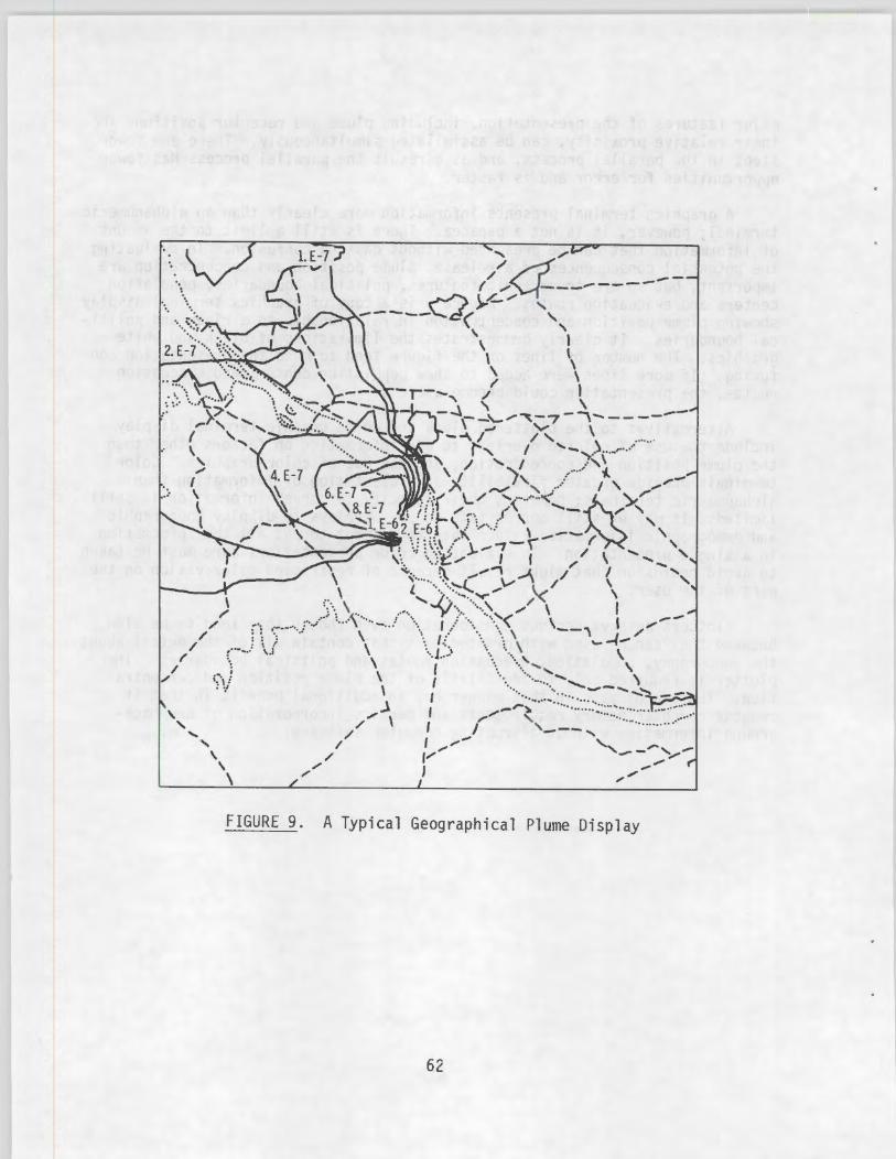
I' I'

/

' '

\ I"

I" I'

1. E -7

"' ' \ \ \

FIGURE 9. A Typical Geographical Plume Display

62

MINICOMPUTER SYSTEM AVAILABILITY

We have discussed the capabilities and reliability of computer systems and system components. Now we consider the availability of minicomputer systems and system components. In this context availability is related to the number of manufacturers and vendors of minicomputers and other system components, and to the time required for delivery, installation and acceptance of the compon­ents and systems.

COMPONENT AVAILABILITY AND PRICE

Computer Business News (September 1, 1980) listed 75 minicomputer manufac­turers. To determine the number of computers with capabilities adequate to be considered for emergency response applications, screening criteria (a) were developed from NRC Guidelines contained in NUREG-0654 and NUREG-0696 and the requirements of atmospheric process models. These criteria are:

• Main memory capacity of 120K bytes • Minimum of 6 simultaneous users • Capacity for more than 18 communications lines • Hard disk storage capability with 1 M byte capacity • Availability of FORTRAN.

Using these criteria 246 minicomputer models from 63 vendors (Datapro Reports, 1980b) and 266 small business computers from 71 vendors (Datapro Reports, 1980a) were evaluated. (Some computers were contained in both lists.) From these computers 95 models from 29 vendors were found to have specifica­tions meeting or exceeding the screening criteria. All of these models may not be currently available, but there are models known to have adequate capabilit­ies that were not included in either set of specifications. Specifications for these 95 models were examined further.

Computational speeds were not reported for the computers, however times required for integer addition were presented. Table 19 shows the distribution of reported add times in microseconds. Maximum possible computer speeds deter­mined from these and times are also presented in the table. The maximum speeds are reciprocals of the add times. Almost 50% of the models passing the screen­ing criteria have maximum possible speeds exceeding 1 MIPS. It is likely that actual speeds are less than l/2 the maximum possible speed.

Examining the computer memories, more than 90% of the systems have memory access times of one microsecond or less, and about 30 percent had cycle times of l/2 microsecond or less. MOS and Core memories were common (Datapro Reports, 1980b). Table 20 shows the percentage availability of memory error detection,

(a) The criteria are not explicitly contained in the guidelines nor are they intended to reflect the results of a thorough analysis of the requirements for any specific installation.

63

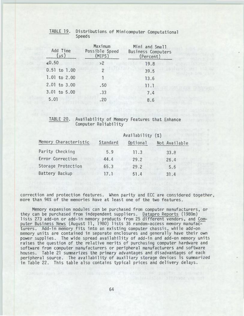
TABLE 19. Distributions of Minicomputer Computational Speeds

Maximum Mini and Sma 11 Add Time Possible Speed Business Computers

( lJS} (MIPS} (Percent} "0.50 >2 19.8 0.51 to 1.00 2 39.5 1.01 to 2.00 1 13.6 2.01 to 3.00 .50 11.1 3.01 to 5.00 .33 7.4 5.01 .20 8.6

TABLE 20. Availability of Memory Features that Enhance Computer Reliability

Availability (%} Memory Characteristic Standard Optional Not Available

Parity Checking 5.9 11.3 33.8 Error Correction 44.4 29.2 26.4 Storage Protection 65.3 29 .2 5.6 Battery Backup 17.1 51.4 31.4

correction and protection features. When parity and ECC are considered together, more than 94% of the memories have at least one of the two features.

Memory expansion modules can be purchased from computer manufacturers, or they can be purchased from independent suppliers. Datapro Reports (1980m) lists 273 add-on or add-in memory products from 25 different vendors, and Com­puter Business News (August 11, 1980) lists 36 random-access memory manufa~ turers. Add-in memory fits into an existing computer chassis, while add-on memory units are contained in separate enclosures and generally have their own power supplies. The wide spread availability of add-in and add-on memory units raises the question of the relative merits of purchasing computer hardware and software from computer manufacturers or peripheral manufacturers and software houses. Table 21 summarizes the primary advantages and disadvantages of each peripheral source. The availabi1ity of auxiliary storage devices is summarized in Table 22. This table also contains typical prices and delivery delays.

64

TABLE 21. Summary of Advantages and Disadvantages of Sources of Peripheral Equipment

Peripheral Source

Computer Manufacturer

Peripheral Manufacturer

l.

2.

l.

2.

Advantaqes

Interfaces already developed Fewer maintenance problems

low price to performance ratio

selection (may be only source of needed device

Disadvantages

l. high cost

2. high prices to performance ratio

l. lack of account-ability if system problems arise

2. maintenance support may not be available

TABLE 22. Auxiliary Storage Devices Availability

Number Number of of Price Range Typical Price Deliver~

( $) (~ ) Typi ca 1 Type of O~_,_Vl:..:::.C.::..e __ _ Hard Disk Orivesa Floppy Disk Drivesb Reel-to-reel Magnetic Tape Unitsc Cassette and Cartridge Magnetic

Tape Uni tsd Punched Paper Tape Unitse Punched Card Unitsf

a) Datapro Reports 1980n b) Datapro Reports, 1980o c) Datapro Reports, 1980e d) Datapro Reports, 1980f e) Datapro Reports, 1980d f) Oatapro Reports, 1980f

Models 247 131

71

85 127

50

Vendors ~ 39 4000-50,000 5,000-1 5,000 30-90 45-60 35 400-15,000 800- 2,000 10-90 30 16 4000-45,000 10,000-20,000 30-120 60-90

17 200-10,000 500- 1 ,500 0-180 30 15 200- 6,000 2,000- 3,000 0-90 45-60 9 400-50,000 2,000- 4,000 30-120 60-90

Input/output device availability is summarized in Table 23. The user programmable terminals and microcomputers are intelligent devices that could be used to provide backup computational and communications capabilities in an emergency response system. The price of these units generally ranges between $5,000 and $15,000 and incJudes memory and floppy disk drives. The 149 micro­computer models listed in Datapro Reports (1980h) were screened using the fol­lowing criteria:

• 8 I/0 ports • 32K byte memory capacity • high level programming language • disk drive, printer and display.

65

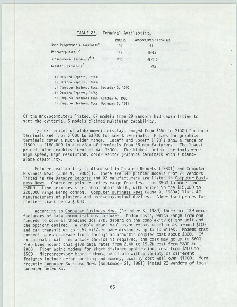
TABLE 23. Terminal Availability

User-Programmable Terminalsa

Microcomputersb,c

Alphanumeric Terminalsd,e

Graphics Terminalsf

a) Datapro Reports, 1980k b) Datapro Reports, 1980h

Models

103

149

210

c) Computer Business News, November 3, 1980 d) Datapro Reports, 1980j e) Computer Business News, October 6, 1980 f) Computer Business Ness, February 9, 1981

Vendors/Manufacturers 52

49/63

68/113

-/73

Of the microcomputers listed, 67 models from 29 vendors had capabilities to meet the criteria; 5 models claimed multiuser capability.

Typical prices of alphanumeric displays ranged from $450 to $1500 for dumb terminals and from $1000 to $3000 for smart terminals. Prices for graphics terminals cover a much wider range. Loceff and Loceff (1981) show a range of $1500 to $180,000 in a review of terminals from 25 manufacturers. The lowest priced color graphics terminal was $2000. The highest priced terminals were high speed, high resolution, color vector graphics terminals with a stand­alone capability.

Printer availability is discussed in Datapro Reports (19801) and Computer Business News (June 9, 1980b)). There are 346 printer models from 71 vendors listed in the Datapro Reports and 97 manufacturers are listed in Computer Busi­ness News. Character printer prices range from less than $500 to more than $5000. Line printers start about about $5000, with prices in the $15,000 to $20,000 range being common. Computer Business News (June 9, 1980a) lists 42 manufacturers of plotters and hard-copy-output devices. Advertised prices for plotters start below $1000.

According to Computer Business News (December 8, 1980) there are 139 manu­facturers of data communications hardware. Modem costs, which range from one hundred to several thousand dollars, depend on the complexity of the unit and the options desired. A simple short haul asynchronous model costs around $100 and can transmit up to 9.6K bit/sec over distances up to 10 miles. Modems that connect to voice-grade lines through an acoustic coupler cost about $300. If an automatic call and answer service is required, the cost may go up to $600. Wide-band modems that give data rates from 2.4K to 19.2K cost from $800 to $900. Fiber optic modems for short distance applications cost from $400 to $500. Microprocessor based modems, available with a variety of different features include error handling and memory, usually cost well over $1000. More recently Computer Business News (September 21, 1981) listed 22 vendors of local computer networks.

66

List prices for minicomputer computer systems {Datapro Reports, l980a and b) range from less than $5,000 to more than $150,000 and are distributed as shown in Table 24. Several factors contribute to this wide range, including differ­ences in the hardware and software included for the price. A number of systems were examined in detail in an attempt to compensate for these differences. The low priced computers are generally limited to a CPU, power supply and possibly some memory. The cost of six models listed at $10,000 to $20,000 increased to the $50,000 to $150,000 range when they were included in full-blown systems with 128 to 512K bytes of memory and peripherals such as disk and tape drives. Simi­lary, the cost of three models listed in the $40,000 to $50,000 range increased to the $150,000 to $220,000 range when included in systems. The prices of the higher priced models increase to the upper end of this same range. In no case did the final system include full implementation of the capabilities set forth in the screening criteria. Discounts offered by some vendors were not considered.

TABLE 24. List Prices for Minicomputers

Number of Price Models

<$20,000 20

$20,001-$40,000 25

$40,001-$60,000 17

$60,001-$80,000 14

$80,001-$100,000 9

>$100,000 10

Total 95

Many of the prices did not include operating systems or high level program­ming languages. In these cases the software must be purchased separately. License fees might also be required. These costs can range from a few hundred to a few thousand dollars for programming languages. Similarly, it may be necessary to purchase software for network and communications control.

DELIVERY, INSTALLATION AND TESTING

Computer specifications are not the only measure of availability, deliv­ery records are also important. Delivery records, relative to dates promised by vendors, are shown in Tables 25 and 26 for minicomputers and mainframes.

67

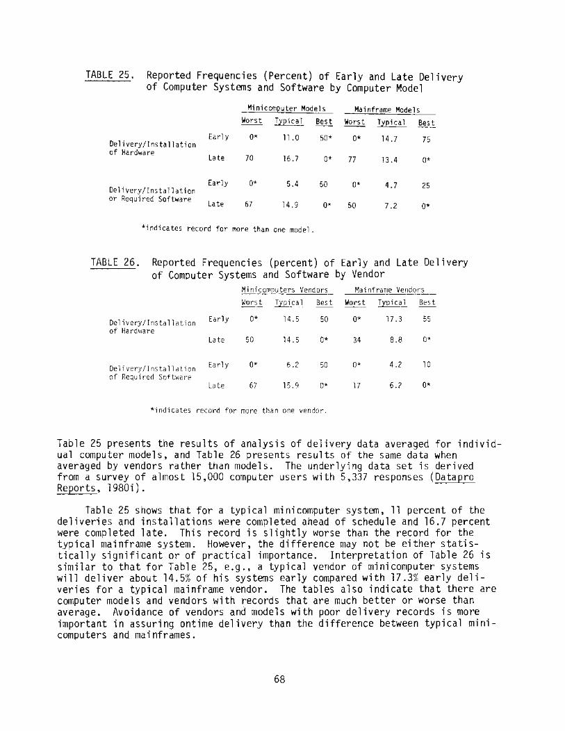
TABLE 25. Reported Frequencies (Percent) of Early and Late Delivery of Computer Systems and Software by Computer Model

Minicom£uter Models Mainframe Models Worst T,t£iCal Best Worst TJ:'£ica 1 Best

Delivery/Installation Early o• 11 .0 so• o• 14.7 75

of Hardware late 70 16.7 o• 77 13 .4 o•

Delivery/Installation Early o• 5.4 50 o• 4.7 25

or Required Software Late 57 14.9 o• 50 7.2 o•

*indicates record for more than one model.

TABLE 26. Reported Frequencies (percent) of Early and Late Delivery of Computer Systems and Software by Vendor

!1.i.Q_i_s_2rJlp_u _ters Vendors -

Mainframe Vei!.QC!_t::~_

Wars t I.l.Q_i cal Best Worst Typica_l Best

De 1 i very /l ns ta 11 at ion Early o• 14.5 50 o• 17.3 55 of Hard\·lare

Late 50 14.5 o• 34 8.8 o•

Deli very/! nsta 1l d lion Early o• 6.2 50 o• 4.2 l 0 of Re~uireti Softwarr

Late 67 15.9 o• 17 6.7 o•

*indicates record for mure than cce vendor.

Table 25 presents the results of analysis of delivery data averaged for individ­ual computer models, and Table 26 presents results of the same data when averaged by vendors rather than models. The underlying data set is derived from a survey of almost 15,000 computer users with 5,337 responses (Datapro Reports, 1980i).

Table 25 shows that for a typical minicomputer system, 11 percent of the deliveries and installations were completed ahead of schedule and 16.7 percent were completed late. This record is slightly worse than the record for the typical mainframe system. However, the difference may not be either statis­tically significant or of practical importance. Interpretation of Table 26 is similar to that for Table 25, e.g., a typical vendor of minicomputer systems will deliver about 14.5% of his systems early compared with 17.3% early deli­veries for a typical mainframe vendor. The tables also indicate that there are computer models and vendors with records that are much better or worse than average. Avoidance of vendors and models with poor delivery records is more important in assuring ontime delivery than the difference between typical mini­computers and mainframes.

68

It is clear from the preceding discussion that the individual components are available for a computer system for environmental modeling in emergencies. However, this does not mean that a system can be ordered, delivered and instal­led and be considered to be operational in a short period of time. In the fol­lowing discussion we will examine some of the required steps in this process. Extensive discussions of system design and the preparation of specifications can be found in Lines (1980) and Weitzman (1980).

Assuming that the decision has been made to purchase a computer system, the initial step involves planning. System functions must be defined and system performance criteria must be established from the characteristics of the expected computational and communications loads. Existing constraints might include interfaces with existing equipment and spatial limitations. Once these external factors have been identified and evaluated, consideration must be given to identification of key system components and their organization. Particular attention should be given to input and output devices. Finally, purchase specifications must be prepared.

The planning process must be done carefully if the system finally installed is to be fully satisfactory. Depending on the staff involved in planning and the sophistication of the system desired, an adequate planning phase might take 4 to 6 months. If review of the system plans is required prior to entering the procurement phase, the time required for planning could take longer.

The procurement process includes: preparation of requests for proposals, bids or quotes; preparation of responses by vendors; evaluation of responses; negotiation, and placement of a purchase order. The time required for comple­tion of the process depends upon the extent to which the licensee assumes sys­tem design responsibility. If the licensee requires vendors to design a com­plete turn-key system to meet functional and performance specifications, it will be necessary to give vendors significantly more time to respond than if the licensee only wants vendors to supply individual hardware components. Simi­larly the tasks of evaluation of vendor response and negotiation will take longer with the purchase of complete systems.

The tradeoff is, of course, in the time required to translate system requirements into a request for proposals. If the licensee assumes design res­ponsibility, this task will take longer because the design must be completed prior to the request for bids to ensure that all necessary components have been identified and are compatible.

Procurement regulations are another factor that must be considered. Pri­vate utilities may have more flexibility in their procurement practices than public utilities. However, it is likely that all licensees will have some minimum time required for this process. It is probably realistic to estimate that 6 months will be required to reach the point where a purchase order is completed.

The time delay between execution of a purchase order and hardware delivery again depends on the role of the licensee. If the licensee is doing the system development, hardware delivery could be completed in 4 to 6 months.

69

However, if the vendor ·is to deliver a turn-key system, additional time must be allowed to mate components, develop and test system software, and perform pre-delivery system checks. These items could delay delivery by 3 to 6 months. These same steps will be required after hardware delivery if the licensee does the system integration. As a result of the time required for planning, procure­ment and system development, the total time between planning initiation and the completion of system installation is likely to be at least 18 months and may exceed 24 months.

The completion of system installation does not signal that the system is, in fact, operational. Before the system can be considered operational, it must undergo acceptance tests, and systems users must be trained.

Longbottom (1980) discusses acceptance tests in detail. He suggests that they consist of demonstrations in which step-by-step procedures are used to show that the system is operating correctly, and cyclic testing in which the complete system is exercised in a way that involves user interactions and maximum system utilization. He lists the following as characteristics of a practical acceptance trial:

• trial should be specified in contract

• cost to purchaser should not be excessive • trial content should be determined by purchaser • trial should be fully documented • vendor should be responsible for investigating all incidents, correcting

faults, or providing acceptable explanation • final hardware and software should be used

• hardware should be free from early failures • compatibility with other systems should be demonstrated • hardware and software performance should be measured where possible.

When completed, the acceptance trials should be followed by a period in which serviceability or availability under normal operating conditions is demon­strated to be within acceptable limits. The entire acceptance testing process may take 4 months or more. Operator training can be accomplished during the latter portion of this period.

70

APPENDIX

ATMOSPHERIC PROCESS MODELS

APPENDIX

ATMOSPHERIC PROCESS MODELS

The selection of a computer system for use in the collection and dissemi­nation of meteorological information related to the transport, diffusion and depletion of material released to the atmosphere should include consideration of the requirements of the atmospheric models to be used. There may be some combinations of acceptable computer systems and acceptable models that do not give an acceptable resultant emergency response capability. For example. a model that gives a timely output on a CDC-7600 computer may not give a timely output on a minicomputer even though it will run on the minicomputer. The objective of this Appendix is to provide the NRC staff a brief description of two of the facets of atmospheric process models that relate directly to com­puter system resource requirements: model type and wind field representation.

We can divide atmospheric process models into three rather broad classes: Gaussian plume models, trajectory models and particle-in-cell models. The com­puter system resources required generally increase in the order given.

The Gaussian plume models treat transport implicitly; the material is assumed to travel in a straight line with the wind. Exposures are computed as a function of distance from the source and the distance from the plume center­line. Frequently, exposure estimates are limited to the center of the plume, although they may also be esimated at fixed locations in the model domain. In a Gaussian plume model, given a release rate, the source and receptor posi­tions, and wind direction, the exposure is a function of wind speed and stabil­ity and is independent of the path between the source and receptor. The expos­ure at receptors is accumulated when the receptor is directly downwind of the source, even though the wind direction might change before the released mater­ial could reach the receptor at the given wind speed. The computational load required to make exposure estimates is minimal, and they can be made quickly using nomograms or a programmable handheld calculator. These models do not tax even the least powerful of the microcomputers.

The next level of sophistication in dispersion modeling involves the use of trajectories. In a trajectory-type dispersion model, a release of material is represented by a sequence of plume segments or puffs. Each segment or puff is permitted to move in response to a wind field and to diffuse about its cen­terline or center-of-mass. Depending on the complexity of the model, the wind field may be a function of time, a function of time and two-dimensional space, or a function of time and three-dimensional space. The computational require­ments of the model depend on the rate at which plume segments or puffs are released, the resolution of the wind field, and the number of points for which exposures are estimated.

A-1

In the third class of models, transport is the dominant process. Dif­fusion is treated by releasing a large number of particles and super-imposing random variations upon the components of the wind transporting each particle. Thus, diffusion is included in the transport model. These models depend on specification of both the mean wind field and the field of sorrie measure of the variation of the instantaneous winds about their mean values. The computa­tional requirements of these models are related to the number of particles released, the resolution of the wind field, and the number of cells into which the particles can be transported. The exposure estimates in these models are derived values based upon particle concentrations rather than values computed directly from release rates and diffusion parameters. As a result, the resolu­tion of particle-in-cell models is limited by the number of particles released. For example, if 103 particles are released per hour and we consider only those cells in which at least 1 particle falls, the total range of possible expos-

ures ranges from 0.1 particle-hours to 104 particle-hours. The practical range of concentrations is more restricted. This limitation tends to result in particle-in-cell models that release very large numbers of particles. There­fore, particle-in-cell models tend to require large memories to keep track of each particle, and also tend to be slow because they must compute a displace­ment for each particle for every model time-step.

This outline of dispersion model characteristics illustrates that wind field models assume an increasingly important role as dispersion model sophis­tication increases from Gaussian plume models to particle-in-cell models. As the importance of the wind field models increases, so do their computational resource and data base requirements. Wind field models range in sophistica­tion from the single straightline transport models used in most nuclear facil­ity licensing studies to approximate solutions of the full set of Navier-Stokes equations in three dimensions. Although there is essentially a continuum of models on the sophistication scale, several basic types can be identified. Nominally these are:

• Unifonn wind field • Area of influence • Empirical interpolation • Objective analysis • Simplified physics • Full physics (primitive equation)

The sophistication increases from top to bottom of the list as do the memory, computational time and data input requirements.

Unifonn wind field (UW) models are common and are used in the NRC licens­ing process to estimate effects of routine re 1 eases. . They. are d~scri bed in detail by Gifford (1968) and in several regulatory gu1des 1nclud1ng Regulatory Guides 1.111 and 1.145. In evaluation of the effects of an accidental release, these models are realistic only in the area where the assumption of a unifonn wind field can be considered valid. At some nuclear facilities this region

A-2

might extend to a distance of 15 to 20 km from the facility, while at other locations the assumption might be valid for no more than 2 or 3 km.

The data input for a transport model consists of uniform wind field based on a single representative wind direction and speed. The direction of trans­port is the reciprocal of the wind direction and speed of movement of the effluent is equal to the wind speed. Thus, computational requirements of the model are minimal and can be met by hand-held calculators, simple nomograms or even look- up tables.

The limitations of UW models are obvious. Straight line transport can lead to plumes passing through mountains or other obstacles. The uniform wind field does not permit a plume trajectory to curve to follow a valley. The only curvature in trajectories results from variations in the wind field with time. One solution is, of course, to permit the wind field to vary in space as well as time.

Area of Influence {AI) models, based on measured winds, are a better, but still simple, approach to describing the wind field. Wind instruments are dis­tributed throughout the region of interest and each is assigned an area of influence within the region. The boundaries between areas are assigned on the basis of physical insight and consideration of probable effects of topographic features. The initial plume transport conforms to the wind speed and direction in the area of release just as it does in a UW model. However, when the plume reaches a boundary between areas it changes direction and speed so its trans­port conforms to the wind in the area that it is entering. In this way curved trajectories are possible without changing the wind field. Hinds (1970) used this approach to estimate transport times in coastal mountains in Southern California with results that appear to be reasonable.

The computational requirements for this approach are quite modest. Essen­tially, they consist of a series of simple estimates of the distance between area boundaries and the time required to transmit each area. It would be rea­sonable to estimate transport with an AI model using a hand calculator or nomographs. Estimating transport in this way might take several minutes compared to a few seconds with a uniform wind field model, but the results should be more realistic.

The limitations on accuracy of an AI model are related to the number of wind measurement sites and the skill with which the area boundaries are drawn. The time required to make transport estimates is primarily related to the speed with which data can be entered into the model. Computational time should be negligible.

The logical extension of the AI model is use of the available data to esti­mate the wind at a large number of points within the field. There are many ways to make the desired estimates. One of the most common techniques is the weighted average interpolation scheme used by Wendell (1972}. Grid point winds are determined by averaging winds from at least three measurement locations. The

A-3

weight assigned in averaging is proportional to the reciprocal of the square of the distance between the grid point and the measurement location. Thus the scheme is strictly empirical, and we call the wind field model an Empirical Interpolation (EI) model.

Typical EI model grids contain more than 100 points (lOxlO). As a result, the computational load implicit in selection or use of an interpolated wind field is more than can be reasonably accomplished by hand following an accident. On the other hand, it is well within the capability of micro- and minicomputers. The computational time required for interpolation depends upon many factors including grid size, computer and skill of the programmer. For modest grids (say 20x20), and typical small computers, it is reasonable to expect the inter­polation to be completed within a few seconds. As with all interpolation schemes, accuracy depends on the amount of data available. MESOI (Ramsdell and Athey, 1g8l), a trajectory dispersion model that uses Wendell's (1972) wind field model, requires fewer than 20K words of memory on a UNIVAC 1100/44 com­puter. Including the time required to initialize the model interactively, the model can simulate a 12 hour release in less than 5 minutes when 6 puffs are released per hour and each puff is moved and exposures are accumulated at 2 minute intervals.

The next level of sophistication in modeling of wind fields comes with the application of physical constraints to the interpolation process. Sherman (1978) Traci, et al. (1977) and have developed Objective Analysis (OA) wind field model approaches that are termed mass consistent. In these models, the con­tinuity equation is imposed as a constraint on the wind field. As a result they are capable of identifying features that might be missed by less sophis­ticated models. However, this resolution is gained at the expense of increased data requirements and computational time.

OA models are typically used with three dimensional grids thereby signifi­cantly increasing the number of grid points for which computations must be made. MATHEW developed by Sherman uses 30,000 grid points, and NOABL (Traci, et al., 1977) uses 37,500 points. Input data required for these models includes terrain elevation for the lower boundary, a wind field at the top of the grid, and initial wind estimates at all grid points. The geostrophic wind may be used at the top of the field, and the surface wind field may be estimated using an empirical scheme similar to Wendell's. An empirical expression relating upper level to observed surface winds or a measured vertical profile of the horizontal wind components may be used to estimate winds between the bottom and top of the grid. The continuity condition is then used to adjust the wind field.

Sherman (1978) reports that MATHEW requires about 200,000 words memory temporary storage and takes several minutes to run on a CDC 7600 computer. NOABL is reported to require about 15 seconds for wind field convergence and about 100,000 words, also on a CDC 7600. Thus, it is evident that these models have been developed primarily for large computers. However, it is possible to run them on some mini- and microcomputers. Ludwig and Byrd (1980) describe a

A-4

technique that substantially reduces the computational time for OA models for climatological studies, but their technique has not been tested for specific uses.

As an alternative to the AI, EI and OA approach, wind field models have been developed by simplification of the Navier-Stokes equations. The model developed by Fosberg, Marlatt and Krupnak (1976) to provide wind fields for predicting fire behavior and evaluation of air pollution transport patterns is typical of the simplified physics (SP) models. It is a 2-dimensional single layer model in which the advection terms in Navier-Stokes equations are neglected and other terms are simplified using first-order assumptions. The model starts with a uniform background wind direction and speed imposed at the top of the layer. The geostrophic wind may be assumed for this purpose. The surface wind field is then derived by successive superposition of disturbances caused by terrain, surface friction and thermal forces.

Input data required by the model include temperature, pressure, terrain elevation and surface roughness at each point in the computational grid. In addition, the background wind direction and speed and an estimate of atmos­pheric stability are required. With a modest grid (50x50), the memory required for this model is less than that required for an objective analysis model. A quantitative estimate of the computational time required is not available, however it is sufficiently short that the model can be used operationally in predicting wind fields near forest fires.

The size of the area modeled is controlled by the terrain roughness, in addition to computer resources. A grid spacing of 6 km has been found to be satisfactory if the maximum difference in terrain elevation within the model domain is less than 300 m. Reduction of spacing of 1 km is recommended for each 300m increase in elevation difference. It is also suggested that the reasonable spacing is 500 m.

The most sophisticated wind field models are the full physics (FP) or pri­mative equation models (PE). These models are based on the Navier-Stokes equations and are three-dimensonal. The SIGMET model (Traci, et al., 1977) and the model developed by Pielke (1974) are typical full physics models. These models require extensive computer resources and are slow running, even on the fastest computers. Computational times for full physics models are generally compared with "real time." A current version of SIGMET runs at about l/2 real time on a CDC 7600, i.e., a l hour simulation requires 30 minutes of run time.

With the exception of the FP models, wind field models are generally diag­nostic. That is, they can be used to estimate the wind field given existing data. The diagnostic nature of the models makes them useful for following the course of an emergency as it evolves, but it limits their application in pre­dicting the future devleopments. These models can be used to estimate future plume positions only to the extent that persistence in the wind field is assumed or forecast atmospheric data are available from other sources. The assumption of persistence for more than 2 to 3 hours is questionable under nor­mal atmospheric conditions. As a result, consideration of the forecasting

A-5

problems presented by each model is important. Is it realistic to make the detailed forecasts that might be required by the more sophisticated models?

A-6

REFERENCES

Brengle, T. A. and N. Maron, 1980. "Comparing the Floating Point Systems, Inc., APL-190L to Representative Scientific Computers; Some Bendwnark Results," UCRL-84095 presented at 1980 Fourth Annual FPS User•s Conference, San Fran­cisco, April 28, 1980.

Computer Business News, June 9, 1980a. 11 Plotter and Hard-Copy-Output Tenninal Manufacturers, 11 p. 12.

Computer Business News, June 9, 1980b. "Printer Manufacturers," p. 10

August 11, 1980. "Semiconductor Random-Access Memory p. 4.

Computer Business News, September 1, 1980. "Minicomputer Manufacturers," p. 10.

Computer Business News, October 6, 1980. 11 Manufacturers of Alphanumeric Display Teminals, 11 p. 16.

Computer Business News, November 3, 1980. "Vendors of Microprocessors, Microcom­puters and Microcomputer Operating and Development Systems, 11 p. 11.

Computer Business News, December 8, 1980. "Data Corrmunications Manufacurers," p. 9.

Computer Business News, February 9, 1981. ''Vendors of Computer Grapics VDTs,' p. 14.

Computer Business News, September 21, 1981. 11 Vendors of Local Area Computer Networks," p. 5.

Conti, D. M., 1978. "U.S. Efforts to Develop Standard Benchmark Programs," Soft­ware World, lQ., No. 2 pp. 2-9.

Conti, D. M., 1979. "Findings of the Standard Benchmark Library Study Group," National Bureau of Standards Special Publication 500-38, PB291779, 53 p.

Datapro Reports on Mini computers, 1979. "Microcomputer Specifications," Oatapro Research Corporation, Delran, N.J.

Datapro Reports on Minicomputers, l980a. "Small Business Computer Specifica­tions," Datapro Research Corporation, Delran, N.J.

Datapro Reports on Mini computers, 1980b. "Mini computers Speci fi cations," Data­pro Research Corporation, Delran, N.J.

Datapro Reports on Minicomputers, 1980c. "Minicomputer Punched Card Units, 11

Datapro Research Corporation, Delran, NJ.

Ref-1

Dataero Reports on Mini computers, 1 980d. "Mini computer Punched Paper- Tape Un1ts, 11 Datapro Research Corporation, Delran, NJ.

Datapro Reports on Minicomputers, l980e. "Minicomputer Reel-to-Reel Magnetic Tape Units, 11 Datapro Research Corporation, Delran, NJ.

Datapro Reports on Minicomputers, 1980f. "Minicomputer Cassette and Cartridge Magnetic Tape Units," Datapro Research Corporation, Delran, NJ.

Datapro Reports on Minicomputers, l980g. "Microprocessor Specifications," Datapro Research Corporation, Delran, NJ.

Datapro Reports on Minicomputers, l980h. "Microcomputer Specifications," Datapro Research Corporation, Delran, NJ.

Datapro Reports on Minicomputers, 1980i. "User Ratings of Computer Systems, 11

Datapro Research Corporation, Delran, NJ.

Datapro Reports on Minicomputers, 1980j. "Alphanumeric Display Terminals," Datapro Research Corporation, Delran, NJ.

Datapro Reports on Minicomputers, 1980k. ''User-Programmable Terminals," Datapro Research Corporation, Delran, NJ.

Datapro Reports on Minicomputers, 19801. "Minicomputer Printers," Datapro Research Corporation, Delran, NJ.

Datapro Reports on Mini computers, l980m. "Mini computer Add-on Memories," Datapro Research Corporation, Delran, NJ.

Datapro Reports on Mini computers, 1980n. "Mini computer Disk Storage," Data­pro Research Corporation, Delran, NJ.

Datapro Reports on Minicomputers, 1980o. "Minicomputer Floppy Disk Storage," Oatapro Research Corporation, Delran, NJ.

Eckhouse, R. H. and L. R. Morris, 1979. Minicomputer Systems, 3nd Ed., Prentice-Hall, Englewood Cliffs, 491 p.

Fosberg, M.A., W. E. Marlatt and l. Krupnak, 1976. "Estimating Airflow Pat­terns Over Complex Terrain," USDA Forest Service Research Paper RM-162, 16 p.

Fox, T., 1980. "Assignment; Benchmark," Interface Age, 5, No.6, p. 130.

Fox, T. 1981. "Report Card: Benchmark," Interface Age, 6, No. 8 p. 74.

Gifford, F. A. 1968. of the Atmosphere,'' ter 3, pp. 65-116.

"An Outline of Theories of Diffusion in the Lower Layers Meteorology and Atomic Energy-1968, TID-24190, Chap-

Ref-2

Hinds, W. T. 1970. "Diffusion over Coastal Mountains of Southern California," Atrnos. Environ.,!· pp. 107-124.

lines, M. V. and Boeing Computer Services Company, 1980. Mini cpmputer Sys terns, Winthrop Publishers, Inc., Cambridge, 217 p.

Loceff, M. and A. loceff, 1981. "Computer Graphics: Manufacturer by Manu­facturer," Interface Age, February, pp. 78-82.

Longbottm, R., 1980. Computer System Reliability, Wiley, New York, 321 p.

Ludwig, F. L. and G. Byrd, 1980. "An Efficient Method for Deriving Mass­Consistent Flow Fields from Wind Observations in Rough Terrain," Atmos. Environ.,}!: 585-587.

McKnight, A. L., 1979. "LASL bendmark Perfonnance 1978," LA-7957-~1S, 6 p.

Myers, W., 1980. ''Computer Grahpics: A Two-Way Street,'' Computer, 13, No. 6, pp. 49-58.

Ohio Scientific, 1981. Advertisements in BYTE, January, p. 386.

Parsons, T. W., 1980. "All About ASCII," Microcomputing 1 November, pp. 129-132.

Pielke, R. A., 1974. "A Three-Dimensional Numerical Model of the Sea Breezes over South Florida," Mon. Wea. Rev., 102:115-139.

Ramsdell, J. V. and G. F. Athey, 1981. MESO!: An Interactive Lagrangian Tra­jectory Puff Diffusion Model, PNL-3998, Pacific Northwest Laboratory, Ric­land, WA. 84 p.

Shennan, C. A., 1978. 11 A Mass-Consistent Model for Wind Fields over Complex Terrain," J. Appl. Meteor., 17:312-319.

Start, G. E. and L. l. Wendell, 1974. Regional Effluent Dispersion Calculations Consideration Spatial and Temporal Meteorological Variations, NOAA Tech. Memo., ERL ARL 44, 63 p.

Traci, R. M., G. T. Phillips, P. C. Patnaik and B. E. Freeman, 1977. ment of a Wind Energy Site Selection methodology," RL0/2440-ll, 205

"Oevelop­p.

U.S. Nuclear Regulatory Commission, 1977. Methods for Estimating Atmospheric Transport and Dispersion of Gaseous Effluents in Routine Releases from Light­Water-Cooled Reactors, Regulatory Guide 1 .lll, Rev. l. USNRC, Washington, DC.

U.S. Nuclear Regulatory Commission, 1979. Atmospheric Dispersion Models for Potential Accident Consequence Assessments at Nuclear Power Plants, Regula­tory Guide 1.145, USNRC, Washington, DC.

Ref-3

U.S. Nuclear Regulatory Commission, 1980. Meteorological Programs in Support of Nuclear Power Plants. Proposed Revision to Regulatory Guide 1.23, OSNRC, Washington, DC.

U.S. Nuclear Regulatory Commission, 1980. Criteria for Preparation and Evalua­tion of Radiological Emergency Response Plans and Preparedness in Support of Nuclear Power Plants, NUREG 0654 Rev. 1, USNRC, Washington, DC.

U.S. Nuclear Regulatory Commission. 1981. Functional Criteria for Emergenc~ Response Facilities, NUREG-0696, USNRC, Washington, DC.

Weitzman, C., 1980. Distributed Micro/Minicomputer Systems, Prentice-Hall, Englewood Cliffs, 403 p.

Wendell, L. L. 1972. "Mesoscale Wind Fields and Transport Estimates Detenni ned from a Network of Wind Towers," Man. Wea. Rev. • 1 00: 565-578.

Ref-4

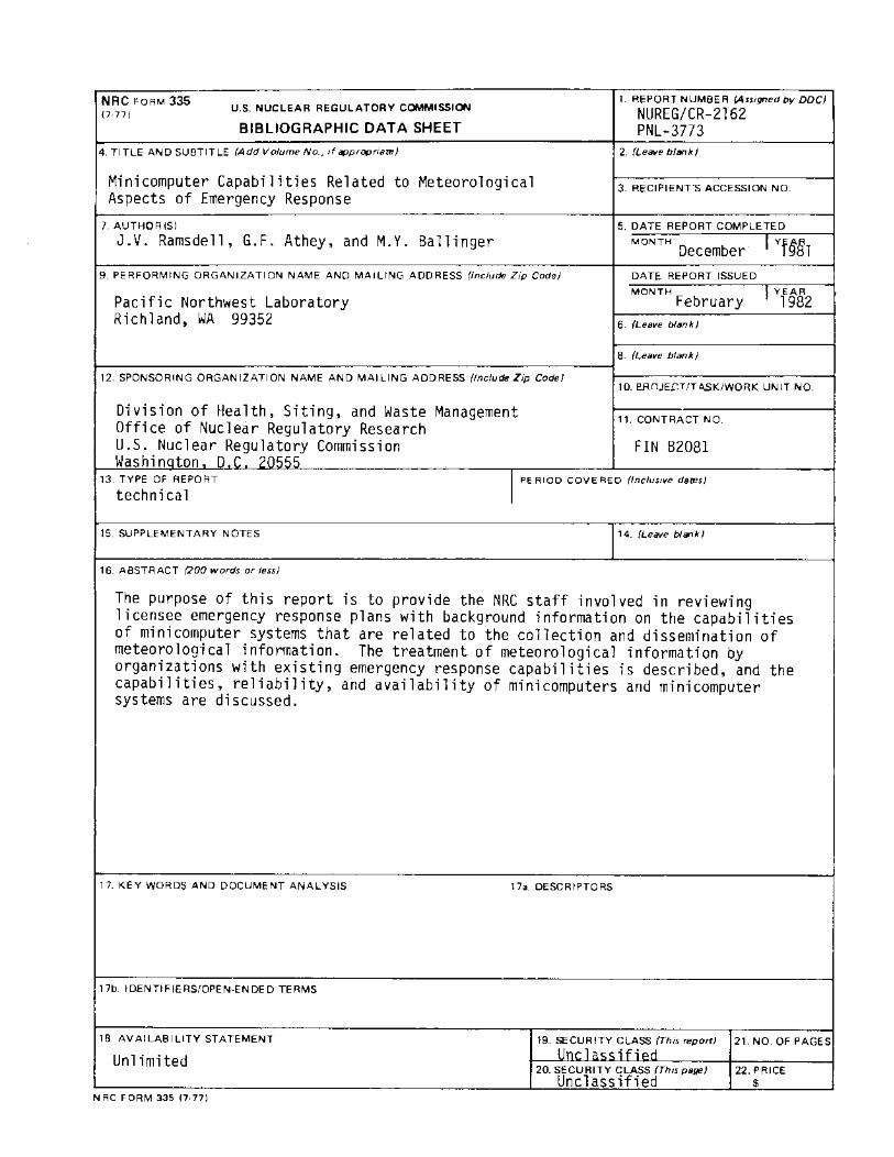
NRC FORM 335 1 REPORT NUMBER {AmgnedbvDDC) U.S. NUCLEAR REGULATORY COMMISSION

NUREG/CR-2162 {7-771

BIBLIOGRAPHIC DATA SHEET PNL-3773 4. TITLE AND SUBTITLE (Add Volume No., d appropoare) 2. (Leave blank)

Minicomputer Capabilities Related to Aspects of Emergency Response

Meteorological 3. RECIPIENT"S ACCESSION NO_

7. AUTHOR lSI 5. DATE REPORT COMPLETED

J. v. Rams de 11, G.F. Athey, and M.Y. Ballinger MONTH I Yf~~ December 1 9_ PERFORMING ORGANIZATION NAME AND MAILING ADDRESS (Include Zip Code) DATE REPORT ISSUED

MONTH Pacific Northwest Laboratory February

! YEAR 1982

Richland, WA 99352 6 (Leave bliJnk/

8. (Leave blank)

12. SPONSORING ORGANIZATION NAME AND MAILING ADDRESS (Include Zip Code/ 1Q_ E'RnJE,r.T/Tto.SK/WORK UNIT NO.

Division of Health, Siting, and Waste Management 11 CONTRACT NO Office of Nuclear Regulatory Research U.S. Nuclearn~~gu~~~~? Commission FIN 82081 Washinaton

13. TYPE OF REPORT I PERIOD COVE REO (lnclus,ve dares)

technical

15. SUPPLEMENTARY NOTES 14_ {Leave blank/

15 ABSTRACT (200 words or less/

The purpose of this report is to provide the NRC staff involved in reviewing 1 i censee emergency response plans with background information on the capabilities of minicomputer systems that are related to the collection and dissemination of meteorological information. The treatment of meteorological information by organizations with existing emergency response capabilities is described, and the capabilities, reliability, and availability of minicomputers and minicomputer systems are discussed.

17. KEY WORDS AND DOCUMENT ANALYSIS 17a DESCRIPTORS

17b IDENTIFIERS/OPEN-ENDED TERMS

18 AVAILABILITY STATEMENT 19. 7T.,C~f~:Y._~~s::hls reporr/ 21 NO OF PAGES

Unlimited 20. SECURITY CLASS (TillS page/ 22. PRICE

Unclassified $ NRC FORM 335 17·771