Minimum independent dominating sets of random cubic graphs

Minimum Independent Dominating Setsof Random Cubic Graphs

W. Duckworth,* N. C. Wormald†Department of Mathematics & Statistics, University of Melbourne, Australia

Received 5 April 2000; revised 6 June 2001; accepted 18 May 2002Published online 00 Month 2002 in Wiley InterScience (www.interscience.wiley.com).DOI 10.1002/rsa.10047

ABSTRACT: We present a heuristic for finding a small independent dominating set � of cubicgraphs. We analyze the performance of this heuristic, which is a random greedy algorithm, onrandom cubic graphs using differential equations, and obtain an upper bound on the expected sizeof �. A corresponding lower bound is derived by means of a direct expectation argument. We provethat � asymptotically almost surely satisfies 0.2641n � �� 0.27942n. © 2002 Wiley Periodicals,Inc. Random Struct. Alg., 21: 147–161, 2002

1. INTRODUCTION

A dominating set S of a graph G is a subset of the vertices of G such that for every vertexv � V(G), S contains either v itself or some neighbor of v in G. An independentdominating set � of a graph G is a dominating set such that no two vertices of � areconnected by and edge of G. We are interested in finding independent dominating sets ofsmall cardinality.

The problem of finding a minimum independent dominating set of a graph is one of thecore, well-known, NP-hard graph-theoretic optimization problems [4]. Halldorsson [5]showed that, for general n-vertex graphs, this problem is not approximable within n1��

for any � � 0. Kann [6] showed that the same problem, when restricted to graphs of

Correspondence to: W. Duckworth; e-mail: [email protected].*Currently in the Department of Computing, Macquarie University, Australia.†Supported by the Australian Research Council.© 2002 Wiley Periodicals, Inc.

147

bounded degree, is APX-complete. Note that, for d-regular graphs, it is simple to verifythat this problem is approximable within (d � 1)/ 2.

Molloy and Reed [8] showed that, for a random n-vertex cubic graph G, the size of asmallest dominating set, D(G), asymptotically almost surely satisfies 0.2636n � �D(G)�� 0.3126n. The algorithm they use to prove their upper bound finds a minimumdominating set in the random 3-regular multigraph formed by taking the union of aHamilton cycle on n vertices and a uniformly selected perfect matching on the samevertex set. The simplistic approach would be to construct the dominating set by choosingevery third vertex around the Hamilton cycle. Molloy and Reed prove their upper boundby modifying this simplistic approach and considering the probability that a vertex isadjacent to a member of the dominating set across a matching edge. A result of Robinsonand Wormald [10] ensures that the result obtained translates to uniformly distributedrandom cubic graphs. Their lower bound is obtained by means of a direct expectationargument.

Reed [9] showed that the size of a minimum dominating set of an n-vertex cubic graphis at most 3n/8 and gave an example of a cubic graph on eight vertices with no dominatingset of size less than 3, demonstrating the tightness of this bound. Lam, Shiu, and Sun [7]recently showed that the size of a minimum independent dominating set of an n-vertexcubic graph is at most 2n/5 and gave an example of a cubic graph on ten vertices with noindependent dominating set of size less than 4.

In this paper, we present a heuristic for finding a small independent dominating set ofcubic graphs. We analyze the performance of this heuristic, which is a random greedyalgorithm, on random n-vertex cubic graphs using differential equations and obtain anupper bound on the expected size of the independent dominating set � returned by thealgorithm. A corresponding lower bound is calculated by means of a direct expectationargument. We show that � asymptotically almost surely satisfies 0.2641n � �� 0.27942n.

A deterministic version of the randomized algorithm that we present in this paper wasanalyzed in [3] using linear programming. It was shown that, given an n-vertex cubicgraph, the deterministic algorithm returns an independent dominating set of size at most29n/70 � O(1) and there exist infinitely many n-vertex cubic graphs for which thealgorithm only attains this bound. In the same paper, it was also shown that there existinfinitely many n-vertex cubic graphs that have no independent dominating set of size lessthan 3n/8.

Throughout this paper we use the notation P (probability), E (expectation), u.a.r.(uniformly at random), and a.a.s. (asymptotically almost surely) (see, for example,Bollobas [1] for these and other random graph theory definitions). When discussing anycubic graph on n vertices, we assume n to be even to avoid parity problems.

In the following section we introduce the model used for generating cubic graphs u.a.r.,and in Section 3 we describe the notion of analyzing the performance of algorithms onrandom graphs using a system of differential equations. Section 4 gives the randomizedalgorithm and Section 5 gives its analysis showing the a.a. sure upper bound. In Section6 we give a direct expectation argument showing the a.a. sure lower bound.

2. GENERATING RANDOM CUBIC GRAPHS

The model used to generate a cubic graph u.a.r. (see, for example, [1]) may be summarizedas follows. For an n-vertex cubic graph

148 DUCKWORTH AND WORMALD

● Take 3n points in n buckets labelled 1 . . . n with three points in each bucket● Choose u.a.r. a disjoint pairing of the 3n points.

If no pair contains two points from the same bucket and no two pairs contain four pointsfrom just two buckets, this represents a cubic graph on n vertices with no loops and nomultiple edges. With probability bounded below by a positive constant, loops and multipleedges do not occur (see, for example, [12, Section 2.2]). The buckets represent the verticesof the randomly generated cubic graph and each pair represents an edge whose end-pointsare given by the buckets of the points in the pair.

We may consider the generation process as follows. Initially, all vertices have degree0. Throughout the execution of the generation process, vertices will increase in degreeuntil the generation is complete and all vertices have degree 3. During this process, werefer to the graph being generated as the evolving graph.

3. ANALYSIS USING DIFFERENTIAL EQUATIONS

One method of analyzing the performance of a randomized algorithm is to use a systemof differential equations to express the expected changes in variables describing the stateof the algorithm during its execution. Wormald [13] gives an exposition of this methodand Duckworth [2] applies this method to various other graph-theoretic optimizationproblems.

The algorithm we use to find an independent dominating set � of cubic graphs is agreedy algorithm based on selecting vertices of given degree. We say that our algorithmproceeds as a series of operations. For each operation, a vertex v is chosen u.a.r. fromthose of current minimum degree. A vertex is chosen to be added to � from v and itsneighbors based on the degree(s) of the neighbor(s) of v. If v has a neighbor of degreestrictly greater than that of v, a vertex is chosen to be added to � u.a.r. from those ofmaximum degree amongst the neighbors of v. Otherwise, we add v to �. The edgesincident with the chosen vertex and its neighbors are then deleted in order to ensure thatthe dominating set remains independent. Any isolated vertices created, which were notneighbors of the chosen independent dominating set vertex, are then added to �. We referto these vertices as accidental isolates.

In order to analyze our algorithm using a system of differential equations, we incor-porate the algorithm as part of a pairing process that generates a random cubic graph. Inthis way, we generate the random graph in the order that the edges are examined by thealgorithm.

During the generation of a random cubic graph, we choose the pairs sequentially. Thefirst point, pi, of a pair may be chosen by any rule, but in order to ensure that the cubicgraph is generated u.a.r., the second point, pj, of that pair must be selected u.a.r. from allthe remaining free (i.e., unpaired) points. The freedom of choice of pi enables us to selectit u.a.r. from the vertices of given degree in the evolving graph. Using B( pk) to denote thebucket that the point pk belongs to, we say that the edge (B( pi), B( pj)) is exposed. Notethat we may then determine the degree of the vertex represented by the bucket B( pj),without exposing any further edges incident with that vertex.

Incorporating our algorithm as part of a pairing process that generates a random cubicgraph, we select a vertex, v, u.a.r. from those of maximum degree in the evolving graphand expose its incident edge(s). A vertex is selected to be added to � based on the

INDEPENDENT DOMINATING SETS OF RANDOM CUBIC GRAPHS 149

degree(s) of the new neighbor(s) of v. Further edges are then exposed in order to ensurethe dominating set remains independent. More detail is given in the following section.

In what follows, we denote the set of vertices of degree i of the evolving graph, at timet, by Vi � Vi(t) and let Yi � Yi(t) denote �Vi�. We can express the state of the evolvinggraph at any point during the execution of the algorithm by considering Y0, Y1, and Y2.In order to analyze our randomized algorithm for finding an independent dominating set� of cubic graphs, we calculate the expected change in this state over one unit of time (aunit of time is defined more clearly in Section 5) in relation to the expected change in thesize of �. Let D � D(t) denote �� at any stage of the algorithm (time t) and let E�Xdenote the expected change in a random variable X conditional upon the history of theprocess. We then regard E�Yi/E�D as the derivative dYi/dD, which gives a system ofdifferential equations. The solutions to these equations describe functions which representthe behavior of the variable Yi. There is a general result which guarantees that thesolutions of the differential equations almost surely approximate the variables Yi. Theexpected size of the independent dominating set may be deduced from these results.

4. THE ALGORITHM

In this section we present the algorithm incorporated with the pairing process, for findingan independent dominating set of a random cubic graph. It is noteworthy that relaxing theindependence condition does not suggest any alternative approach along similar lines, soin some sense we get independence for free.

We denote the set of all free points in the evolving graph by P and use q(b) to denotethe set of free points in a given bucket b. The combined algorithm and pairing process,RANDMIDS, is given below:

select u u.a.r. from V0;� 4 {u};E 4 { }isolate(u);Add any accidental isolates to �;while (Y1 � Y2 � 0){

if (Y2 � 0)select v u.a.r. from V2;{ p1} 4 q(v);select p2 u.a.r. from P;u 4 B( p2);add the edge uv to E;

elseselect v u.a.r. from V1;{ p1, p2} 4 q(v);select p3 u.a.r. from P;j 4 b( p3);select p4 u.a.r. from P;k 4 b( p4);add vj and vk to E;

if ( j � V2 � k � V1) u 4 k;


else if ( j � V1 � k � V2) u 4 j;else if ( j � V2 � k � V2) u 4 v;else select u u.a.r. from { j, k};� 4 � � {u};isolate(u);Add any accidental isolates to �;

}

When the algorithm terminates, as we see below, � is the independent dominating setof the graph, whose edge set is E. The function isolate(b) involves the process ofexposing all edges incident with b and its neighbors (including adding those edges to E).This is achieved by randomly selecting a mate for each free point of b and then exposingall edges incident with free points in the buckets of these selected mates. Note that whenisolate(b) is applied, the accidental isolates are just all vertices which enter V3 but are notb or its neighbors.

It is straightforward to verify that � is, in the end, an independent dominating set ofthe graph. To see that it is dominating, note that all vertices enter V3 eventually. Thoseentering V3 other than as accidental isolates, are either a vertex being added to � or oneof its neighbors. All accidental isolates are also placed in �, so � is dominating. Forindependence, note that vertices can only enter � from V0, V1 or V2. The functionisolate(b) ensures that for any vertex b to which it is applied, all neighbors of b enter V3

without entering �. So the only possible edges between vertices in � are those betweenaccidental isolates. However, as every edge added to the graph is incident with a vertexentering V3 inside the function isolate(b) (either b or one of its neighbors), accidentalisolates cannot be adjacent to each other.

The algorithm terminates when there are no vertices of degree 1 or 2 remaining, whichmeans that a connected component has been completely generated, and an independentdominating set has been found in that component. It is well known that a random cubicgraph is a.a.s. connected, so the result is a.a.s. an independent dominating set in the wholegraph.

The first operation of the algorithm is the operation that randomly selects the firstvertex of the independent dominating set. We split the remainder of the algorithm into twodistinct phases. We informally define Phase 1 as the period of time where any vertices inV2 that are created are used up almost immediately and Y2 remains small. Once the rateof generating vertices in V2 becomes larger than the rate that they are used up, thealgorithm moves into Phase 2 and all operations involve selecting a vertex from V2. Thetransition point between phases is not obvious but arises in our analysis.

There are two types of operation performed by the algorithm. Figure 1 shows thepreferred selection of independent dominating set vertex for a typical operation when avertex is chosen from V1 and we shall call this Type 1. Similarly we have Fig. 2 when avertex is chosen from V2, and we shall call this Type 2. In both cases the independentdominating set vertex is chosen as to maximize the number of edges exposed.

The larger circles represent buckets with the points of that bucket represented bysmaller circles. Points that were (without a doubt) free (respectively used up) at the startof an operation are colored black (respectively white). Other points are shaded. In allcases, the selected vertex is labelled v and the independent dominating set vertex chosenis labelled u. Vertices of unknown degree at the start of an operation are labelled eitherw or p. We refer to these vertices as rems (for “remove”) and incs (for “increase”),respectively. An inc will have its degree increased by 1 for the next operation of the


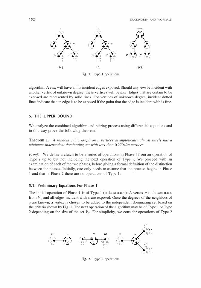
algorithm. A rem will have all its incident edges exposed. Should any rem be incident withanother vertex of unknown degree, these vertices will be incs. Edges that are certain to beexposed are represented by solid lines. For vertices of unknown degree, incident dottedlines indicate that an edge is to be exposed if the point that the edge is incident with is free.

5. THE UPPER BOUND

We analyze the combined algorithm and pairing process using differential equations andin this way prove the following theorem.

Theorem 1. A random cubic graph on n vertices asymptotically almost surely has aminimum independent dominating set with less than 0.27942n vertices.

Proof. We define a clutch to be a series of operations in Phase i from an operation ofType i up to but not including the next operation of Type i. We proceed with anexamination of each of the two phases, before giving a formal definition of the distinctionbetween the phases. Initially, one only needs to assume that the process begins in Phase1 and that in Phase 2 there are no operations of Type 1.

5.1. Preliminary Equations For Phase 1

The initial operation of Phase 1 is of Type 1 (at least a.a.s.). A vertex v is chosen u.a.r.from V1 and all edges incident with v are exposed. Once the degrees of the neighbors ofv are known, a vertex is chosen to be added to the independent dominating set based onthe criteria shown by Fig. 1. The next operation of the algorithm may be of Type 1 or Type2 depending on the size of the set V2. For simplicity, we consider operations of Type 2

Fig. 1. Type 1 operations

Fig. 2. Type 2 operations


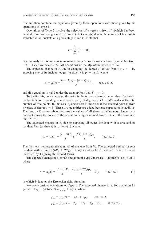
first and then combine the equations given by these operations with those given by theoperations of Type 1.

Operations of Type 2 involve the selection of a vertex v from V2 (which has beencreated from processing a vertex from V1). Let s � s(t) denote the number of free pointsavailable in all buckets at a given stage (time t). Note that

s � �i�0

2

�3 � i�Yi.

For our analysis it is convenient to assume that s � �n for some arbitrarily small but fixed� � 0. Later we discuss the last operations of the algorithm, when s � �n.

The expected change in Yi due to changing the degree of an inc from i to i � 1 byexposing one of its incident edges (at time t) is �i � o(1), where

�i � �i�t� ��i � 3�Yi � �4 � i�Yi�1

s, 0 � i � 2,

and this equation is valid under the assumptions that Y�1 � 0.To justify this, note that when the point in the inc was chosen, the number of points in

the buckets corresponding to vertices currently of degree i is (3 � i)Yi, and s is the totalnumber of free points. In this case Yi decreases; it increases if the selected point is froma vertex of degree i � 1. These two quantities are added because expectation is additive.The term o(1) comes about because the values of all these variables may change by aconstant during the course of the operation being examined. Since s � �n, the error is infact O(1/n).

The expected change in Yi due to exposing all edges incident with a rem and itsincident incs (at time t) is �i � o(1) where

�i � �i�t� ��i � 3�Yi

s�

�6Y0 � 2Y1��i

s, 0 � i � 2.

The first term represents the removal of the rem from Vi. The expected number of incsincident with a rem is (6Y0 � 2Y1)/s � o(1) and each of these will have its degreeincreased by 1 (giving the second term).

The expected change in Yi for an operation of Type 2 in Phase 1 (at time t) is �i � o(1)where

�i � �i�t� ��i � 3�Yi

s�

�6Y0 � 2Y1��i

s� i2, 0 � i � 2 (1)

in which denotes the Kronecker delta function.We now consider operations of Type 1. The expected change in Yi for operation 1h

given in Fig. 1 (at time t) is h,i � o(1), where

a,i � a,i�t� � �2io � 2�i, 0 � i � 2,

b,i � b,i�t� � �i0 � 2i1 � i2 � 2�i, 0 � i � 2,


c,i � c,i�t� � �3i1 � 2�i, 0 � i � 2.

For an operation of Type 1 in Phase 1, neighbors of v (the vertex selected at randomfrom V1) were in {V0 � V1} at the start of the operation, since Y2 � 0 when thealgorithm performs this type of operation. The probability that these neighbors were in V0

or V1 are asymptotically 3Y0/s and 2Y1/s, respectively. Therefore, the probabilities that,given we are performing an operation of Type 1 in Phase 1, the operation is that of type1a, 1b, or 1c are given by

P�1a� �9Y0

2

s2 � o�1�,

P�1b� �12Y0Y1

s2 � o�1�,

P�1c� �4Y1

2

s2 � o�1�,

respectively.We define a birth to be the generation of a vertex in V2 by processing a vertex of V1

or V2 in Phase 1. The expected number of births from processing a vertex from V1 (at timet) is �1 � o(1), where

�1 � �1�t� �9Y0

2

s2 � 2�2 �12Y0Y1

s2 � �1 � 2�2� �4Y1

2

s2 �4Y1

s.

Here, for each case, we consider the probability that vertices of degree 1 (in the evolvinggraph) become vertices of degree 2 by exposing an edge incident with the vertex.

Similarly, the expected number of births from processing a vertex from V2 (at time t)is �2 � o(1) where

�2 � �2�t� ��6Y0 � 2Y1��2

s.

Consider the Type 1 operation at the start of the clutch to be the first generation of abirth–death process in which the individuals are the vertices in V2, each giving birth toa number of children (essentially independent of the others) with expected number �2.Then, the expected number in the jth generation is �1� 2

j�1 and the expected total numberof births in the clutch is

�1

1 � �2.

For Phase 1, the equation giving the expected change in Yi for a clutch is thereforegiven by


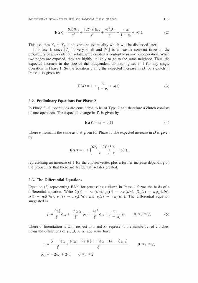
E�Yi �9Y0

2a,i

s2 �12Y0Y1b,i

s2 �4Y1

2c,i

s2 ��1�i

1 � �2� o�1�. (2)

This assumes Y1 � Y2 is not zero, an eventuality which will be discussed later.In Phase 1, since �V2� is very small and �V1� is at least a constant times n, the

probability of an accidental isolate being created is negligible in any one operation. Whentwo edges are exposed, they are highly unlikely to go to the same neighbor. Thus, theexpected increase in the size of the independent dominating set is 1 for any singleoperation in Phase 1. So the equation giving the expected increase in D for a clutch inPhase 1 is given by

E�D � 1 ��1

1 � �2� o�1�. (3)

5.2. Preliminary Equations For Phase 2

In Phase 2, all operations are considered to be of Type 2 and therefore a clutch consistsof one operation. The expected change in Yi is given by

E�Yi � �i � o�1� (4)

where �i remains the same as that given for Phase 1. The expected increase in D is givenby

E�D � 1 � �6Y0 � 2Y1

s �2 Y2

s� o�1�,

representing an increase of 1 for the chosen vertex plus a further increase depending onthe probability that there are accidental isolates created.

5.3. The Differential Equations

Equation (2) representing E�Yi for processing a clutch in Phase 1 forms the basis of adifferential equation. Write Yi(t) � nzi(t/n), �i(t) � n i(t/n), j,i(t) � n�j,i(t/n),s(t) � n�(t/n), �i(t) � n�i(t/n), and �j(t) � n�j(t/n). The differential equationsuggested is

z�i �9z0

2

�2 �a,i �12z0z1

�2 �b,i �4z1

2

�2 �c,i ��1

1 � �2�i, 0 � i � 2, (5)

where differentiation is with respect to x and xn represents the number, t, of clutches.From the definitions of �, , s, �, and � we have

i ��i � 3�zi

��

�6z0 � 2z1��i � 3�zi � �4 � i�zi�1�

�2 , 0 � i � 2,

�a,i � �2i0 � 2 i, 0 � i � 2,


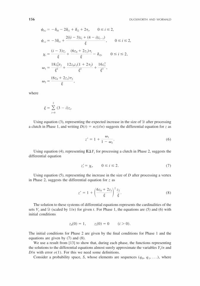
�b,i � �i0 � 2i1 � i2 � 2 i, 0 � i � 2,

�c,i � �3i1 �2��i � 3�zi � �4 � i�zi�1�

�, 0 � i � 2,

�i ��i � 3�zi

��

�6z0 � 2z1� i

�� i2, 0 � i � 2,

�1 �18z0

2 2

�2 �12z0z1�1 � 2 2�

�2 �16z1

3

�3 ,

�2 ��6z0 � 2z1� 2

�,

where

� � �i�0

2

�3 � i�zi.

Using equation (3), representing the expected increase in the size of � after processinga clutch in Phase 1, and writing D(t) � nz(t/n) suggests the differential equation for z as

z� � 1 ��1

1 � �2. (6)

Using equation (4), representing E�Yi for processing a clutch in Phase 2, suggests thedifferential equation

z�i � �i, 0 � i � 2. (7)

Using equation (5), representing the increase in the size of D after processing a vertexin Phase 2, suggests the differential equation for z as

z� � 1 � �6z0 � 2z1

� � 2 z2

�. (8)

The solution to these systems of differential equations represents the cardinalities of thesets Vi and � (scaled by 1/n) for given t. For Phase 1, the equations are (5) and (6) withinitial conditions

z0�0� � 1, zi�0� � 0 �i � 0�.

The initial conditions for Phase 2 are given by the final conditions for Phase 1 and theequations are given by (7) and (8).

We use a result from [13] to show that, during each phase, the functions representingthe solutions to the differential equations almost surely approximate the variables Yi/n andD/n with error o(1). For this we need some definitions.

Consider a probability space, S, whose elements are sequences (q0, q1, . . .), where


each qt � S. We use ht to denote (q0, q1, . . . , qt), the history of the process up to timet, and Ht for its random counterpart. S(n)� denotes the set of all ht � (q0, . . . , qt) whereeach qi � S, t � 0, 1, . . . . All these things are indexed by n and we will considerasymptotics as n 3 .

We say that a function f(u1, . . . , uj) satisfies a Lipschitz condition on W � �j if aconstant L � 0 exists with the property that

�f�u1, . . . , uj� � f�v1, . . . , vj�� L max1�i�j

�ui � vi�

for all (u1, . . . , uj) and (v1, . . . , vj) in W, and note that max1�i�j�ui � vi� is thedistance between (u1, . . . , uj) and (v1, . . . , vj) in the � metric.

For variables Y1, . . . , Ya defined on the components of the process, and W � �a�1,define the stopping time TW � TW(Y1, . . . , Ya) to be the minimum t such that (t/n,Y1(t)/n, . . . , Ya(t)/n) � W.

The following is a restatement of [13, Theorem 6.1]. We refer the reader to that paperfor explanations, and to [11] for a similar result with virtually the same proof.

Theorem 2. Let W � W(n) � �a�1. For 1 � l � a, where a is fixed, let yl : S(n)� 3� and fl : �a�13 �, such that for some constant C0 and all l, �yl(hl)� C0n for all hl �S(n)� for all n. Let Yl(t) denote the random counterpart of yl(hl). Assume the followingthree conditions hold, where in (ii) and (iii) W is some bounded connected open setcontaining the closure of

��0, z1, . . . , za� : P�Yl�0� � zln, 1 � l � a� � 0 for some n�.

(i) For some functions � (n) � 1 and � � �(n), the probability that

max1�l�a

�Yl�t � 1� � Yl�t�� .

conditional upon Hl, is at least 1 � � for t min{TW, TW}.(ii) For some function �1 � �1(n) � o(1), for all l � a,

�E�Yl�t � 1� � Yl�t��Hl� � fl�t/n, Y1�t�/n, . . . , Ya�t�/n�� 1

for t min{TW, TW}.(iii) Each function fl is continuous, and satisfies a Lipschitz condition, on

W � ��t, z1, . . . , za� : t � 0�.

with the same Lipschitz constant for each l.

Then the following are true:

(a) For (0, z1, . . . , za) � W the system of differential equations

dzl

dx� fl�x, z1, . . . , za�, l � 1, . . . , a

has a unique solution in W for zl : � 3 � passing through

zl�0� � zl,


1 � l � a, and which extends to points arbitrarily close to the boundaryof W.

(b) Let � � �1 � C0n� with � � o(1). For a sufficiently large constant C, with

probability 1 � O(n� � � exp(� n�3

3)),

Yl�t� � nzl�t/n� � O��n�

uniformly for 0 � t � min{�n, TW} and for each l, where zl( x) is the solutionin (a) with zl � 1

n Yl(0), and � � �(n) is the supremum of those x to whichthe solution can be extended before reaching within �-distance C� of theboundary of W.

First, we apply Theorem 2 to the Process within Phase 1. For arbitrary small �, defineW to be the set of all (t, z0, z1, z2, z) for which t � ��, � � �, �2 1 � �, z � ��,and zi 1 � �, where 0 � i � 2. Also define W to be the vectors for which z1 � 0,z2 � 0, and z1 � z2 � 0.

For part (i) of Theorem 2 we must ensure that Yi(t) does not change too quicklythroughout the process. As long as the expected number of births in a clutch is boundedabove, the probability of getting say n� births is O(n�K) for any fixed K. This comes froma standard argument as in [13, p. 141]. So part (i) of Theorem 2 holds with � n� and� � n�K. Near the start of the process, operations may be of Type 1 or Type 2. Equations(2) and (3) verify part (ii) for a function �1 which goes to zero sufficiently slowly. (Notein particular that since � � � inside W, the assumption that s � �n used in deriving theseequations is justified. Also, since t TW, it follows that Y1 � Y2 � 0, so that the nextoperation is of Type 1 or Type 2.) Part (iii) of Theorem 2 is immediate from the form ofthe functions in Eqs. (2) and (3).

The conclusion of Theorem 2 therefore holds. This implies (taking �3 0 sufficientlyslowly) that the random variables Yi/n and D/n a.a.s. remain within o(1) of the corre-sponding deterministic solutions to the differential Eqs. (5) and (6) until a point arbitrarilyclose to where it leaves the set W, or until t � TW if that occurs earlier. Since the lattercan only occur when the algorithm has completely processed a component of the graph,and a random cubic graph is a.a.s. connected, we may turn to examining the former.

We compute the ratio dzi/dz � z�i( x)/z�( x), and we have

dzi

dz�

9z02

�2 �a,i �12z0z1

�2 �b,i �4z1

2

�2 �c,i ��1

1 � �2�i

1 ��1

1 � �2

, 0 � i � 2, (9)

where differentiation is with respect to z and all functions can be taken as functions of z.By solving (numerically) this system of differential equations, we find that the solution

hits a boundary of the domain at �2 � 1 � � (for � � 0 this would be at z � 0.1375).At this point, we may formally define Phase 1 as the period of time from time t � 0 tothe time t0 such that z � t0/n is the solution of �2 � 1.

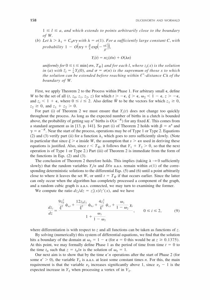
Our next aim is to show that by the time ��n operations after the start of Phase 2 (forsome �� 0), the variable Y2 is a.a.s. at least some constant times n. For this, the mainrequirement is that the variable �2 increases significantly above 1, since �2 � 1 is theexpected increase in Y2 when processing a vertex of in V2.


Unfortunately, the expected increase in �2 due to processing a vertex from V1 right nearthe end of Phase 1 is negative. So instead we consider the variable �2 defined by settingY2 � 0 in the definitions of all variables; that is,

� 2 � � 2�t� ��6Y0 � 2Y1�� 2

s,

where

� 2 � � 2�t� ��6Y0 � 2Y1�� 2

s,

� 2 � � 2�t� �2Y1

s,

s � 3Y0 � 2Y1.

Regarding �2 as a function of Y0 and Y1 only, we may compute the expected increasein �2 due to an operation of Type 1 as

�� 2

�Y0E0 �

�� 2

�Y1E1, (10)

where Ei is the expected increase in Yi in such an operation. The latter can be computedfrom the first three terms on the right side of (2). Plugging in the values of Y0 and Y1 atthe end of Phase 1 gives a positive quantity, approximately 3.86. For a Type 2 operation,the same calculation is used, but the values of E0 and E1 come from �i as seen in (2). Theresult is 3.93.

Since the formula given by (10) is Lipschitz, it must remain positive for at least �1noperations after reaching time t0 � �n, for �1 sufficiently small. Subject to the choice of�1, we may take � arbitrarily small. It now follows by the usual large deviation argumentthat the increase in �2 between time t0 � �n and a time t1 when �1n operations haveoccurred in Phase 2 is a.a.s. at least c for some positive constant c. By choosing �sufficiently small, �2 is a.a.s. arbitrarily close to 1 at time t0 � �n, and so the same goesfor �2 since Y2 is a.a.s. very small in Phase 1. Thus �2 � 1 � c1 a.a.s. at time t1 for somec1 � 0.

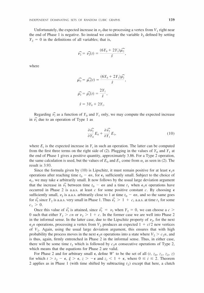
Once this value of �2 is attained, since �2 � �2 when Y2 � 0, we can choose a c �0 such that either Y2 � cn or �2 � 1 � c. In the former case we are well into Phase 2in the informal sense. In the latter case, due to the Lipschitz property of �2, for the next�2n operations, processing a vertex from V2 produces an expected 1 � c/ 2 new verticesof V2. Again, using the usual large deviation argument, this ensures that with highprobability the process moves in the next �2n operations into a state where V2 � c2n, andis thus, again, firmly entrenched in Phase 2 in the informal sense. Thus, in either case,there will be some time t2 which is followed by c2n consecutive operations of Type 2,which means that the equations for Phase 2 are valid.

For Phase 2 and for arbitrary small �, define W� to be the set of all (t, z0, z1, z2, z)for which t � t2 � �, � � �, z � �� and zi 1 � �, where 0 � i � 2. Theorem2 applies as in Phase 1 (with time shifted by subtracting t2) except that here, a clutch


consists of just one operation of Type 2. Note also that the starting point of the processis randomized, which is permitted in Theorem 2. Computing the ratio dzi/dz � z�i( x)/z�( x) gives

dzi

dz�

�i

1 � �6z0 � 2z1

� � 2 z2

s

, 0 � i � 2.

By solving this we see that the solution hits a boundary of W� at � � � (for � � 0 thiswould be approximately 0.27942n).

The differential equations were solved using a Runge–Kutta method, giving �2 � 1 atz � 0.1375 and in Phase 2, z2 � 0 at z � 0.27942. This corresponds to the size of theindependent dominating set (scaled by 1/n) when all vertices are used up, thus proving thetheorem. �

6. THE LOWER BOUND

We now establish a lower bound on the size of a minimum independent dominating set ofa random cubic graph.

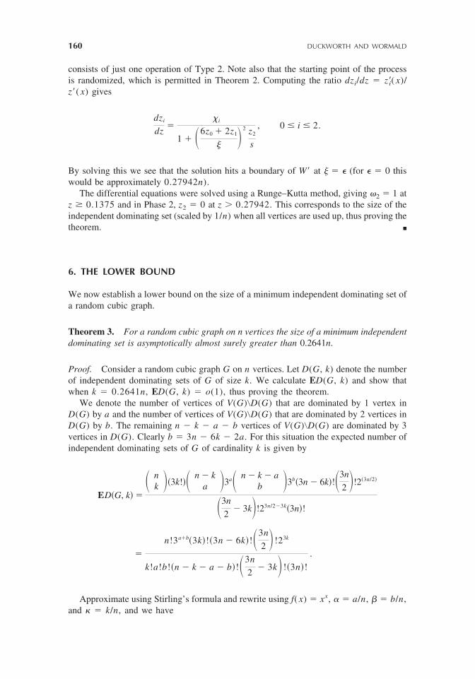
Theorem 3. For a random cubic graph on n vertices the size of a minimum independentdominating set is asymptotically almost surely greater than 0.2641n.

Proof. Consider a random cubic graph G on n vertices. Let D(G, k) denote the numberof independent dominating sets of G of size k. We calculate ED(G, k) and show thatwhen k � 0.2641n, ED(G, k) � o(1), thus proving the theorem.

We denote the number of vertices of V(G)�D(G) that are dominated by 1 vertex inD(G) by a and the number of vertices of V(G)�D(G) that are dominated by 2 vertices inD(G) by b. The remaining n � k � a � b vertices of V(G)�D(G) are dominated by 3vertices in D(G). Clearly b � 3n � 6k � 2a. For this situation the expected number ofindependent dominating sets of G of cardinality k is given by

ED�G, k� �

� nk ��3k!�� n � k

a �3a� n � k � ab �3b�3n � 6k�!�3n

2 �!2�3n/2�

�3n

2� 3k�!23n/2�3k�3n�!

�

n!3a�b�3k�!�3n � 6k�!�3n

2 � !23k

k!a!b!�n � k � a � b�!�3n

2� 3k� !�3n�!

.

Approximate using Stirling’s formula and rewrite using f( x) � xx, � � a/n, � b/n,and � � k/n, and we have


�ED�G, k��1/n �3��f�3��f�3 � 6��f�3

2�23�

f��f��f��f�1 � � � � � �f�3

2� 3��f�3�

.

Substitute for and we have

ED�G, k�)1/n �33�6��f�3��f�3 � 6��f�3

2�23�

f��f��f�3 � 6� � 2��f�� 5� � 2�f�3

2� 3��f�3�

. (11)

We can now differentiate the expression on the right with respect to � and use this to findthat for � � 0.2641 it is strictly less than 1. �

REFERENCES

[1] B. Bollobas, Random graphs, Academic, London, 1985.

[2] W. Duckworth, Greedy algorithms and cubic graphs, Ph.D. thesis, Department of Mathematicsand Statistics, University of Melbourne, Australia, 2001.

[3] W. Duckworth and N. C. Wormald, Linear programming and the worst-case analysis of greedyalgorithms on cubic graphs, in preparation.

[4] M. R. Garey and D. S. Johnson, Computers and intractability: A guide to the theory ofNP-completeness, Freeman, San Francisco, 1979.

[5] M. M. Halldorsson, Approximating the minimum maximal independence number, Inf ProcessLett 46(4) (1993), 169–172.

[6] V. Kann, On the approximability of NP-complete optimisation problems, Ph.D. thesis, De-partment of Numerical Analysis, Royal Institute of Technology, Stockholm, 1992.

[7] P. C. B. Lam, W. C. Shiu, and L. Sun, On the independent domination number of regulargraphs, Discrete Math 202 (1999), 135–144.

[8] M. Molloy and B. Reed, The dominating number of a random cubic graph, Random Struct Alg7(3) (1995), 209–221.

[9] B. Reed, Paths, stars and the number three, Combinat Probab Comput 5 (1996), 277–295.

[10] R. W. Robinson and N. C. Wormald, Almost all cubic graphs are Hamiltonian, Random StructAlg 3(7) (1992), 117–125.

[11] N. C. Wormald, Differential equations for random processes and random graphs, Ann ApplProbab 5 (1995), 1217–1235.

[12] N. C. Wormald, Models of random regular graphs, Surveys in combinatorics, 1999 (Canter-bury), Cambridge University Press, Cambridge, 1999, pp. 239–298.

[13] N. C. Wormald, “The differential equation method for random graph processes and greedyalgorithms,” Lectures on approximation and randomized algorithms, M. Karonski and H. J.Promel (Editors), PWN, Warsaw, 1999, pp. 73–155.


Documents

Minimum independent dominating sets of random cubic graphs