1

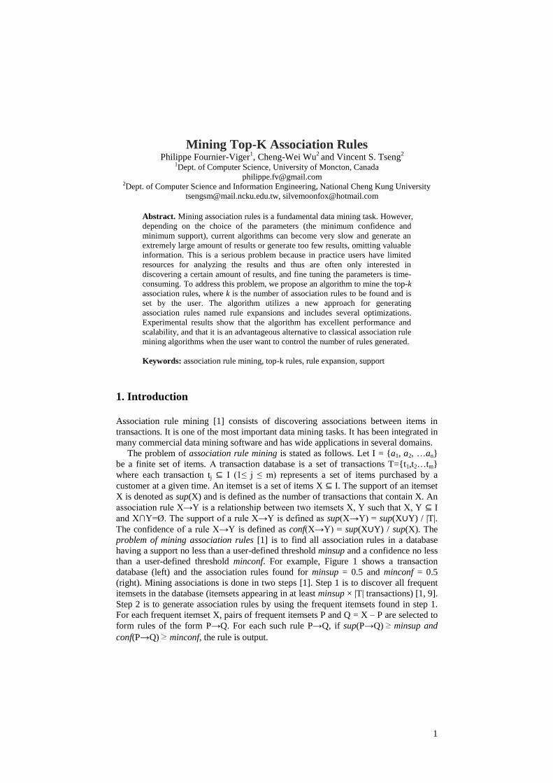
Mining Top-K Association Rules Philippe Fournier-Viger

1, Cheng-Wei Wu

2 and Vincent S. Tseng

2

1Dept. of Computer Science, University of Moncton, Canada

philippe.fv@gmail.com 2Dept. of Computer Science and Information Engineering, National Cheng Kung University

tsengsm@mail.ncku.edu.tw, silvemoonfox@hotmail.com

Abstract. Mining association rules is a fundamental data mining task. However,

depending on the choice of the parameters (the minimum confidence and

minimum support), current algorithms can become very slow and generate an

extremely large amount of results or generate too few results, omitting valuable

information. This is a serious problem because in practice users have limited

resources for analyzing the results and thus are often only interested in

discovering a certain amount of results, and fine tuning the parameters is time-

consuming. To address this problem, we propose an algorithm to mine the top-k

association rules, where k is the number of association rules to be found and is

set by the user. The algorithm utilizes a new approach for generating

association rules named rule expansions and includes several optimizations.

Experimental results show that the algorithm has excellent performance and

scalability, and that it is an advantageous alternative to classical association rule

mining algorithms when the user want to control the number of rules generated.

Keywords: association rule mining, top-k rules, rule expansion, support

1. Introduction

Association rule mining [1] consists of discovering associations between items in

transactions. It is one of the most important data mining tasks. It has been integrated in

many commercial data mining software and has wide applications in several domains.

The problem of association rule mining is stated as follows. Let I = {a1, a2, …an}

be a finite set of items. A transaction database is a set of transactions T={t1,t2…tm}

where each transaction tj ⊆ I (1≤ j ≤ m) represents a set of items purchased by a

customer at a given time. An itemset is a set of items X ⊆ I. The support of an itemset

X is denoted as sup(X) and is defined as the number of transactions that contain X. An

association rule X→Y is a relationship between two itemsets X, Y such that X, Y ⊆ I

and X∩Y=Ø. The support of a rule X→Y is defined as sup(X→Y) = sup(X∪Y) / |T|.

The confidence of a rule X→Y is defined as conf(X→Y) = sup(X∪Y) / sup(X). The

problem of mining association rules [1] is to find all association rules in a database

having a support no less than a user-defined threshold minsup and a confidence no less

than a user-defined threshold minconf. For example, Figure 1 shows a transaction

database (left) and the association rules found for minsup = 0.5 and minconf = 0.5

(right). Mining associations is done in two steps [1]. Step 1 is to discover all frequent

itemsets in the database (itemsets appearing in at least minsup × |T| transactions) [1, 9].

Step 2 is to generate association rules by using the frequent itemsets found in step 1.

For each frequent itemset X, pairs of frequent itemsets P and Q = X – P are selected to

form rules of the form P→Q. For each such rule P→Q, if sup(P→Q)≥ minsup and

conf(P→Q)≥ minconf, the rule is output.

2

Although many studies have been done on this topic (e.g. [2, 3, 4]), an important

problem that has not been addressed is how the user should choose the thresholds to

generate a desired amount of rules. This problem is important because in practice users

have limited resources (time and storage space) for analyzing the results and thus are

often only interested in discovering a certain amount of rules, and fine tuning the

parameters is time-consuming. Depending on the choice of the thresholds, current

algorithms can become very slow and generate an extremely large amount of results or

generate none or too few results, omitting valuable information. To solve this problem,

we propose to mine the top-k association rules, where k is the number of association

rules to be found and is set by the user.

This idea of mining top-k association rules presented in this paper is analogous to

the idea of mining top-k itemsets [10] and top-k sequential patterns [7, 8, 9] in the field

of frequent pattern mining. Note that although some authors have previously used the

term “top-k association rules”, they did not use the standard definition of an

association rule. KORD [5, 6] only finds rules with a single item in the consequent,

whereas the algorithm of You et al. [11] consists of mining association rules from a

stream instead of a transaction database. In this paper, our contribution is to propose an

algorithm for the standard definition (with multiple items, from a transaction database).

To achieve this goal, a question is how to combine the concept of top-k pattern

mining with association rules? For association rule mining, two thresholds are used.

But, in practice minsup is much more difficult to set than minconf because minsup

depends on database characteristics that are unknown to most users, whereas minconf

represents the minimal confidence that users want in rules and is generally easy to

determine. For this reason, we define “top-k” on the support rather than the confidence.

Therefore, the goal in this paper is to mine the top-k rules with the highest support that

meet a desired confidence. Note however, that the presented algorithm can be adapted

to other interestingness measures. But we do not discuss it here due to space limitation.

ID Transactions ID Rules Support Confidence

t1 {a, b, c, e, f, g} r1 {a}→ {b} 0.75 1

t2 {a, b, c, d, e, f} r2 {a}→ {c, e, f} 0.5 0.6

t3 {a, b, e, f} r3 {a, b}→ {e, f} 0.75 1

t4 {b, f, g} … … … …

Fig. 1. (a) A transaction database and (b) some association rules found

Mining the top-k association rules is challenging because a top-k association rule

mining algorithm cannot rely on both thresholds to prune the search space. In the worst

case, a naïve top-k algorithm would have to generate all rules to find the top-k rules,

and if there is d items in a database, then there can be up to 123 dd

rules to consider

[1]. Second, top-k association rule mining is challenging because the two steps process

to mine association rules [1] cannot be used. The reason is that Step 1 would have to be

modified to mine frequent itemsets with minsup = 0 to ensure that all top-k rules can

be generated in Step 2. Then, Step 2 would have to be modified to be able to find the

top-k rules by generating rules and keeping the top-k rules. However, this approach

would pose a huge performance problem because no pruning of the search space is

done in Step 1, and Step 1 is by far more costly than Step 2 [1]. Hence, an important

challenge for defining a top-k association rule mining algorithm is to define an

efficient approach for mining rules that does not rely on the two steps process.

3

In this paper, we address the problem of top-k association rule mining by proposing

an algorithm named TopKRules. This latter utilizes a new approach for generating

association rules named “rule expansions” and several optimizations. An evaluation of

the algorithm with datasets commonly used in the literature shows that TopKRules has

excellent performance and scalability. Moreover, results show that TopKRules is an

advantageous alternative to classical association rule mining algorithms for users who

want to control number of association rules generated. The rest of the paper is

organized as follows. Section 2 defines the problem of top-k association rule mining

and related definitions. Section 3 describes TopKRules. Section 4 presents the

experimental evaluation. Finally, Section 5 presents the conclusion.

2. Problem Definition and Preliminary Definitions

In this section, we formally define the problem of mining top-k association rules and

introduce important definitions used by TopKRules.

Definition 1. The problem of top-k association rule mining is to discover a set L

containing k rules in T such that for each rule r L | conf(r) ≥ minconf, there does not

exist a rule s L | conf(s) ≥ minconf ∧ sup(s) > sup(r).

Definition 2. A rule X→Y is of size p*q if |X| = p and |Y| = q. For example, the size

of {a} → {e, f} is 1*2. Moreover, we say that a rule of size p*q is larger than a rule

of size r*s if p > r and q ≥ s, or if p ≥ r and q > s.

Definition 3. An association rule r is frequent if sup(r) ≥ minsup.

Definition 4. An association rule r is valid if sup(r) ≥ minsup and conf(r) ≥ minconf.

Definition 5. The tid set of an itemset X is as defined tids(X) = {t | t ∊ T ∧ X ⊆ t}.

For example, tids({a, b}) for the transaction database of Figure 1(a) is {t1, t2, t3}.

Definition 6. The tid set of an association rule X→Y is denoted as tids(X→Y) and

defined as tids(X∪Y). The support and confidence of X→Y can be expressed in terms

of tid sets as: sup(X→Y) = |tids(X∪Y)| / |T|, conf(X→Y) = |tids(X∪Y)| / |tids(X)|.

Property 1. For any rule X→Y, tids(X→Y) ⊆ tids(X) ∩ tids(Y).

3. The TopKRules Algorithm

The TopKRules algorithm takes as input a transaction database, a number k of rules

that the user wants to discover, and the minconf threshold.

The algorithm main idea is the following. TopKRules first sets an internal minsup

variable to 0. Then, the algorithm starts searching for rules. As soon as a rule is found,

it is added to a list of rules L ordered by the support. The list is used to maintain the

top-k rules found until now. Once k valid rules are found, the internal minsup variable

is raised to the support of the rule with the lowest support in L. Raising the minsup

value is used to prune the search space when searching for more rules. Thereafter,

each time a valid rule is found, the rule is inserted in L, the rules in L not respecting

4

minsup anymore are removed from L, and minsup is raised to the value of the least

interesting rule in L. The algorithm continues searching for more rules until no rule

are found, which means that it has found the top-k rules.

To search for rules, TopKRules does not rely on the classical two steps approach to

generate rules because it would not be efficient as a top-k algorithm (as explained in

the introduction). The strategy used by TopKRules instead consists of generating

rules containing a single item in the antecedent and a single item in the consequent.

Then, each rule is recursively grown by adding items to the antecedent or consequent.

To select the items that are added to a rule to grow it, TopKRules scans the

transactions containing the rule to find single items that could expand its left or right

part. We name the two processes for expanding rules in TopKRules left expansion

and right expansion. These processes are applied recursively to explore the search

space of association rules.

Another idea incorporated in TopKRules is to try to generate the most promising

rules first. This is because if rules with high support are found earlier, TopKRules can

raise its internal minsup variable faster to prune the search space. To perform this,

TopKRules uses an internal variable R to store all the rules that can be expanded to

have a chance of finding more valid rules. TopKRules uses this set to determine the

rules that are the most likely to produce valid rules with a high support to raise

minsup more quickly and prune a larger part of the search space.

Before presenting the algorithm, we present some important definitions/properties.

Definition 7. A left expansion is the process of adding an item i ∊ I to the left side of a

rule X→Y to obtain a larger rule X∪{i}→Y.

Definition 8. A right expansion is the process of adding an item i ∊ I to the right side

of a rule X→Y to obtain a larger rule X→Y∪{i}.

Property 2. Let i be an item. For rules r: X→Y and r’: X ∪{i}→Y, sup(r) ≥ sup(r’).

Property 3. Let i be an item. For rules r: X→Y and r’: X →Y∪{i}, sup(r) ≥ sup(r’).

Properties 2 and 3 imply that the support of a rule is anti-monotonic with respect to

left and right expansions. In other words, performing any combinations of left/right

expansions of a rule can only result in rules having a support that is less than the

original rule. Therefore, all the frequent rules (cf. Definition 3) can be found by

recursively performing expansions on frequent rules of size 1*1. Moreover, properties

2 and 3 guarantee that expanding a rule having a support less than minsup will not

result in a frequent rule. The confidence of a rule, however, is not anti-monotonic

with respect to left and right expansions, as the next two properties states.

Property 4. If an item i is added to the left side of a rule r:X→Y, the confidence of

the resulting rule r’ can be lower, higher or equal to the confidence of r.

Property 5. Let i be an item. For rules r: X→Y and r’: X→Y∪{i}, conf(r) ≥ conf(r’).

The TopKRules algorithm relies on the use of tids sets (sets of transaction ids) [1]

to calculate the support and confidence of rules obtained by left or right expansions.

Tids sets have the following property with respect to left and right expansions.

Property 6. ∀ r’ obtained by a left or a right expansion of a rule r, tids(r’) ⊆ tids(r).

5

The algorithm. The main procedure of TopKRules is shown in Figure 2. The

algorithm first scans the database once to calculate tids({c}) for each single item c in

the database (line 1). Then, the algorithm generates all valid rules of size 1*1 by

considering each pair of items i, j, where i and j each have at least minsup×|T| tids (if

this condition is not met, clearly, no rule having at least the minimum support can be

created with i, j) (line 2). The supports of the rules {i}→{j} and {j}→{i} are simply

obtained by dividing |tids(i→ j)| by |T| and |tids(j→ i)| by |T| (line 3 and 4). The

confidence of the rules {i}→{j} and {j}→{i} is obtained by dividing |tids(i→ j)| by

|tids(i)| and |tids(j→ i)| by | tids(j)| (line 5 and 6). Then, for each rule {i}→{j} or

{j}→{i} that is valid, the procedure SAVE is called with the rule and L as parameters

so that the rule is recorded in the set L of the current top-k rules found (line 7 to 9).

Also, each rule {i}→{j} or {j}→{i} that is frequent is added to the set R, to be later

considered for expansion and a special flag named expandLR is set to true for each

such rule (line 10 to 12).

TOPKRULES(T, k, minconf) R := Ø. L := Ø. minsup := 0. 1. Scan the database T once to record the tidset of each item.

2. FOR each pairs of items i, j such that |tids(i)| ×|T| ≥ minsup and |tids(j)| ×|T| ≥ minsup: 3. sup({i}→{j}) := |tids(i) ∩ tids(j)| / |T |.

4. sup({j}→{i}) := |tids(i) ∩ tids(j)| / |T|.

5. conf({i}→{j}) := |tids(i) ∩ tids(j)| / |tids(i)|. 6. conf({j}→{i}) := |tids(i) ∩ tids(j)| / |tids(j)|.

7. IF sup({i}→{j}) ≥ minsup THEN 8. IF conf({i}→{j}) ≥ minconf THEN SAVE({i}→{j}, L, k, minsup).

9. IF conf({j}→{i}) ≥ minconf THEN SAVE({j}→{i}, L, k, minsup).

10. Set flag expandLR of {i}→{j}to true. 11. Set flag expandLR of {j}→{i}to true.

12. R := R∪{{i}→{j}, {j}→{i}}. 13. END IF

14. END FOR

15. WHILE ∃r ∈ R AND sup(r) ≥ minsup DO 16. Select the rule rule having the highest support in R 17. IF rule.expandLR = true THEN

18. EXPAND-L(rule, L, R, k, minsup, minconf).

19. EXPAND-R(rule, L, R, k, minsup, minconf). 20. ELSE EXPAND-R(rule, L, R, k, minsup, minconf).

21. REMOVE rule from R.

22. REMOVE from R all rules r ∈ R | sup(r) <minsup.

23. END WHILE

Fig. 2. The TopKRules algorithm

After that, a loop is performed to recursively select the rule r with the highest

support in R such that sup(r) ≥ minsup and expand it (line 15 to 23). The idea is to

always expand the rule having the highest support because it is more likely to

generate rules having a high support and thus to allow to raise minsup more quickly

for pruning the search space. The loop terminates when there is no more rule in R

with a support higher than minsup. For each rule, a flag expandLR indicates if the rule

should be left and right expanded by calling the procedure EXPAND-L and

EXPAND-R or just left expanded by calling EXPAND-L. For all rules of size 1*1,

this flag is set to true. The utility of this flag for larger rules will be explained later.

The SAVE procedure. Before describing the procedure EXPAND-L and

EXPAND-LR, we describe the SAVE procedure (shown in Figure 3). Its role is to

6

raise minsup and update the list L when a new valid rule r is found. The first step of

SAVE is to add the rule r to L (line 1). Then, if L contains more than k rules and the

support is higher than minsup, rules from L that have exactly the support equal to

minsup can be removed until only k rules are kept (line 3 to 5). Finally, minsup is

raised to the support of the rule in L having the lowest support. (line 6). By this

simple scheme, the top-k rules found are maintained in L.

SAVE(r, R, k, minsup)

1. L := L∪{r}. 2. IF |L| ≥ k THEN

3. IF sup(r) > minsup THEN

4. WHILE |L| > k AND ∃s ∈ L| sup(s) = minsup, REMOVE s from L. 5. END IF

6. Set minsup to the lowest support of rules in L.

7. END IF

Fig. 3. The SAVE procedure

Now that we have described how rules of size 1*1 are generated and the

mechanism for maintaining the top-k rules in L, we explain how rules of size 1*1 are

expanded to find larger rules. Without loss of generality, we can ignore the top-k

aspect for the explanation and consider the problem of generating all valid rules. To

find all valid rules by recursively performing rule expansions, starting from rules of

size 1*1, two problems had to be solved.

The first problem is how we can guarantee that all valid rules are found by

left/right expansions by recursively performing expansions starting from rules of size

1*1. The answer is found in properties 2 and 3, which states that the support of a rule

is anti-monotonic with respect to left/right expansions. This implies that all rules can

be discovered by recursively performing left/right expansions starting from frequent

rules of size 1*1. Moreover, these Properties imply that infrequent rules should not be

expanded because they will not lead to valid rules. However, no similar pruning can

be done for confidence because the confidence of a rule is not anti-monotonic with

respect to left expansions (Property 4).

The second problem is how we can guarantee that no rules are found twice by

recursively making left/right expansions. To guarantee this, two sub-problems had to

be solved. First, if we grow rules by performing left/right expansions recursively,

some rules can be found by different combinations of left/right expansions. For

example, consider the rule {a, b} →{c, d}. By performing, a left and then a right

expansion of {a} → {c}, one can obtain the rule {a, b} → {c, d}. But this rule can

also be obtained by performing a right and then a left expansion of {a} → {c}. A

simple solution to avoid this problem is to not allow performing a right expansion

after a left expansion but to allow performing a left expansion after a right expansion.

The second sub-problem is that rules can be found several times by performing

left/right expansions with different items. For instance, consider {b, c}→{d}. A left

expansion of {b}→{d} with item c can result in the rule {b, c}→{d}. But that latter

rule can also be found by performing a left expansion of {c}→{d} with b. To solve

this problem, we chose to only add an item to an itemset of a rule if the item is greater

than each item in the itemset according to the lexicographic ordering. In the previous

example, this would mean that item c would be added to the antecedent of {b}→{d}.

7

But b would not be added to the antecedent of {c}→{d} since b is lexically smaller

than c. By using this strategy and the previous one, no rule is found twice.

The EXPAND-L and EXPAND-R procedures. We now explain how EXPAND-

L and EXPAND-R have been implemented based on these strategies.

EXPAND-R is shown in Figure 4. It takes as parameters a rule I→J to be

expanded, L, R, k, minsup and minconf. To expand the rule I→J, EXPAND-R has to

identify items that can expand the rule I→J to produce a valid rule. By exploiting the

fact that any valid rule has to be a frequent rule, we can decompose this problem into

two sub-problems, which are (1) determining items that can expand a rule I→J to

produce a frequent rule and (2) assessing if a frequent rule obtained by an expansion

is valid. The first sub-problem is solved as follows. To identify items that can expand

a rule I→J and produce a frequent rule, the algorithm scans each transaction tid from

tids(I∩J) (line 1). During this scan, for each item c ∈ I appearing in transaction tid, the

algorithm adds tid to a variable tids(I→J∪{c}) if c is lexically larger than all items in

J (this latter condition is to ensure that no duplicated rules will be generated, as

explained). When the scan is completed, for each item c such that |tids(I→J∪{c})| /

|T| ≥ minsup, the rule I→J∪{c} is deemed frequent and is added to the set R so that it

will be later considered for expansion (line 2 to 4). Note that the flag expandLR of

each such rule is set to false so that each generated rule will only be considered for

right expansions (to make sure that no rule is found twice by different combinations

of left/right expansions, as explained). Finally, the confidence of each frequent rule

I→J∪{c} is calculated to see if the rule is valid, by dividing |tids(I→J∪{c})| by

|tids(I)|, the value tids(I) having already been calculated for I→J (line 5). If the

confidence of I→J∪{c} is no less than minconf, the rule is valid and the procedure

SAVE is called to add the rule to the list L of the current top-k rules (line 5 to 7).

EXPAND-R(I→J, L, R, k, minsup, minconf)

1. FOR each tid ∈ tids(I∩J), scan the transaction tid. For each item c ∈ I appearing in transaction tid that

is lexically larger than all items in J, record tid in a variable tids(I→J∪{c}).

2. FOR each item c where | tids (I→J∪{c})| / |T| ≥ minsup :

3. Set flag expandLR of I→J∪{c} to false.

4. R := R∪{I→J∪{c}}.

5. IF |tids(I→J∪{c})| / |tids(I)| ≥ minconf THEN SAVE(I→J∪{c}, L, k, minsup).

6. END FOR

Fig. 4. The EXPAND-R procedure

EXPAND-L is shown in Figure 5. It takes as parameters a rule I→J to be

expanded, L, R, k, minsup and minconf. Because this procedure is very similar to

EXPAND-R, it will not be described in details. The only extra step that is performed

compared to EXPAND-R is that for each rule I∪{c}→J obtained by the expansion of

I→J with an item c, the value tids(I∪{c}) necessary for calculating the confidence is

obtained by intersecting tids(I) with tids(c). This is shown in line 4 of Figure 5.

Implementing TopKRules efficiently. To implement TopKRules efficiently, we

have used three optimizations, which improve its performance in terms of execution

time and memory by more than an order of magnitude. Due to space limitation, we

only mention them briefly. The first optimization is to use bit vectors for representing

tidsets and database transactions (when the database fits into memory). The benefits

of using bit vectors is that it can greatly reduce the memory used and that the

8

intersection of two tidsets can be done very efficiently with the logical AND

operation [13]. The second optimization is to implement L and R with data structures

supporting efficient insertion, deletion and finding the smallest element and maximum

element. In our implementation, we used a Fibonacci heap for L and R. It has an

amortized time cost of O(1) for insertion and obtaining the minimum, and O(log(n))

for deletion [12]. The third optimization is to sort items in each transaction by

descending lexicographical order to avoid scanning them completely when searching

for an item c to expand a rule.

EXPAND-L(I→J, L, R, k, minsup, minconf)

1. FOR each tid ∈ tids(I∩J), scan the transaction tid. For each item c ∈ J appearing in transaction tid that

is lexically larger than all items in I, record tid in a variable tids(I∪{c}→J)

2. FOR each item c where | tids (I∪{c}→J)| / |T| ≥ minsup :

3. Set flag expandLR of I∪{c} →J to true.

4. tids(I∪{c})| = tids(I) ∩ tids(c).

5. SAVE(I∪{c}→J, L, k, minsup).

6. IF |tids(I∪{c}→J)| / |tids(I∪{c})| ≥ minconf THEN R := R∪{I∪{c}→J}.

7. END FOR

Fig. 5. The EXPAND-L procedure

4. Evaluation

We have implemented TopKRules in Java and performed experiments on a computer

with a Core i5 processor running Windows XP and 2 GB of free RAM. The source

code can be downloaded from http://www.philippe-fournier-viger.com/spmf/.

Experiments were carried on real-life and synthetic datasets commonly used in the

association rule mining literature, namely T25I10D10K, Retail, Mushrooms, Pumsb,

Chess and Connect. Table 1 summarizes their characteristics

Table 1. Datasets’ Characteristics

Datasets Number of

transactions

Number of

distinct items

Average

transaction size

Chess 3,196 75 37

Connect 67,557 129 43

T25I10D10K 10,000 1,000 25

Mushrooms 8,416 128 23

Pumsb 49,046 7,116 74

Influence of the k parameter. We first ran TopKRules with minconf = 0.8 on

each dataset and varied the parameter k from 100 to 2000 to evaluate its influence on

the execution time and the memory requirement of the algorithm. Results are shown

in Table 2 for k=100, 1000 and 2000. Execution time is expressed in seconds and the

maximum memory usage is expressed in megabytes. Our first observation is that the

execution time and the maximum memory usage is reasonable for all datasets (in the

worst case, the algorithm took just a little bit more than six minutes to terminate and 1

GB of memory). Furthermore, when the results are plotted on a chart, we can see that

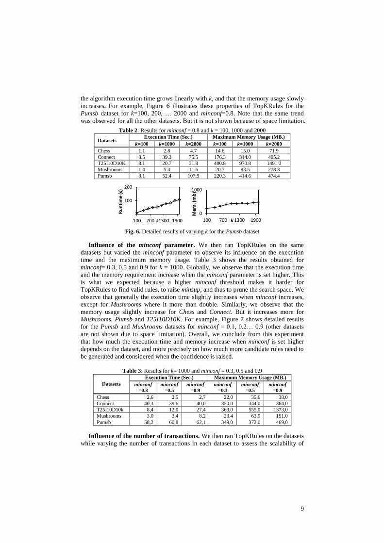
9

the algorithm execution time grows linearly with k, and that the memory usage slowly

increases. For example, Figure 6 illustrates these properties of TopKRules for the

Pumsb dataset for k=100, 200, … 2000 and minconf=0.8. Note that the same trend

was observed for all the other datasets. But it is not shown because of space limitation.

Table 2: Results for minconf = 0.8 and k = 100, 1000 and 2000

Datasets Execution Time (Sec.) Maximum Memory Usage (MB.)

k=100 k=1000 k=2000 k=100 k=1000 k=2000

Chess 1.1 2.8 4.7 14.6 15.0 71.9

Connect 8.5 39.3 75.5 176.3 314.0 405.2

T25I10D10K 8.1 20.7 31.8 400.8 970.8 1491.0

Mushrooms 1.4 5.4 11.6 20.7 83.5 278.3

Pumsb 8.1 52.4 107.9 220.3 414.6 474.4

Fig. 6. Detailed results of varying k for the Pumsb dataset

Influence of the minconf parameter. We then ran TopKRules on the same

datasets but varied the minconf parameter to observe its influence on the execution

time and the maximum memory usage. Table 3 shows the results obtained for

minconf= 0.3, 0.5 and 0.9 for k = 1000. Globally, we observe that the execution time

and the memory requirement increase when the minconf parameter is set higher. This

is what we expected because a higher minconf threshold makes it harder for

TopKRules to find valid rules, to raise minsup, and thus to prune the search space. We

observe that generally the execution time slightly increases when minconf increases,

except for Mushrooms where it more than double. Similarly, we observe that the

memory usage slightly increase for Chess and Connect. But it increases more for

Mushrooms, Pumsb and T25I10D10K. For example, Figure 7 shows detailed results

for the Pumsb and Mushrooms datasets for minconf = 0.1, 0.2… 0.9 (other datasets

are not shown due to space limitation). Overall, we conclude from this experiment

that how much the execution time and memory increase when minconf is set higher

depends on the dataset, and more precisely on how much more candidate rules need to

be generated and considered when the confidence is raised.

Table 3: Results for k= 1000 and minconf = 0.3, 0.5 and 0.9

Datasets

Execution Time (Sec.) Maximum Memory Usage (MB.)

minconf

=0.3

minconf

=0.5

minconf

=0.9

minconf

=0.3

minconf

=0.5

minconf

=0.9

Chess 2,6 2,5 2,7 22,0 35,6 38,0

Connect 40,3 39,6 40,0 350,0 344,0 364,0

T25I10D10k 8,4 12,0 27,4 369,0 555,0 1373,0

Mushrooms 3,0 3,4 8,2 23,4 63,9 151,0

Pumsb 58,2 60,8 62,1 349,0 372,0 469,0

Influence of the number of transactions. We then ran TopKRules on the datasets

while varying the number of transactions in each dataset to assess the scalability of

100

200

100 700 1300 1900

Ru

nti

me

(s)

k

0

1000

100 700 1300 1900

Me

m. (

mb

)

k

10

the algorithm. For this experiment, we used k=2000, minconf=0.8 and 70%, 85 % and

100 % of the transactions in each dataset. Results are shown in Figure 8. Globally we

found that for all datasets, the execution time and memory usage increased more or

less linearly. This shows that the algorithm has an excellent scalability.

Pumsb

Mushrooms

Fig. 7. Detailed results of varying minconf for pumsb and mushrooms

Fig. 8. Influence of the number of transactions on execution time and maximum memory usage

Influence of the optimizations. We next evaluated the benefit of using the three

optimizations described in section 3. To do this, we run TopKRules on Mushrooms

for minconf =0.8 and k=100, 200, … 2000. Due to space limitation, we do not show

the detailed results. But we found that TopKRules without optimization cannot be run

for k > 300 within the 2GB memory limit. Furthermore, using bit vectors has a huge

impact on the execution time and memory usage (the algorithm becomes up to 15

times faster and uses up to 20 times less memory). Moreover, using the lexicographic

ordering and heap data structure reduce the execution time by about 20% to 40 %

each. Results were similar for the other datasets and while varying other parameters.

Performance comparison. Next, to evaluate the benefit of using TopKRules, we

compared its performance with the Java implementation of the Agrawal & Srikant

two steps process [1] from the SPMF data mining framework (http://goo.gl/xa9VX).

This implementation is based on FP-Growth [9], a state-of-the-art algorithm for

mining frequent itemsets. We refer to this implementation as “AR-FPGrowth”.

Because AR-FPGrowth and TopKRules are not designed for the same task (mining

all association rules vs mining the top-k rules), it is difficult to compare them. To

provide a comparison of their performance, we considered the scenario where the user

would choose the optimal parameters for AR-FPGrowth to produce the same amount

of result as TopKRules. We ran TopKRules on the different datasets with minconf =

0.1 and k = 100, 200, … 2000. We then ran AR-FPGrowth with minsup equals to the

lowest support of rules found by TopKRules, for each k and each dataset. Due to

0

50

100

0,1 0,3 0,5 0,7 0,9Ru

nti

me

(s)

minconf

0

500

0,1 0,3 0,5 0,7 0,9

Me

m. (

mb

)

minconf

0

1

0,1 0,3 0,5 0,7 0,9Ru

nti

me

(s)

minconf

0

5

10

0,1 0,3 0,5 0,7 0,9

Me

m. (

mb

) minconf

0

200

400

70% 85% 100%

Ru

nti

me

(s)

Database size

0

2000

4000

0 0 0

Me

m. (

mb

)

Database size

pumsbmushroomsmushroomsconnectchess

11

space limitation, we only show the results for the Chess dataset in Figure 9. Results

for the other datasets follow the same trends. The first conclusion from this

experiment is that for an optimal choice of parameters, AR-FPGrowth is always faster

than TopKRules and uses less memory. Also, as we can see in Figure 9, for smaller

values of k (e.g. k=100), TopKRules is almost as fast as AR-FPGrowth, but as k

increases, the gap between the two algorithms increases.

Fig. 9. Performance comparison for optimal minsup values for chess.

These results are excellent considering that the parameters of AR-FPGrowth were

chosen optimally, which is rarely the case in real-life because it requires possessing

extensive background knowledge about the database. If the parameters of AR-

FPGrowth are not chosen optimally, AR-FPGrowth can run much slower than

TopKRules, or generate too few or too many results. For example, consider the case

where the user wants to discover the top 1000 rules with minconf ≥ 0.8 and do not

want to find more than 2000 rules. To find this amount of rules, the user needs to

choose minsup from a very narrow range of values. These values are shown in Table

4 for each dataset. For example, for the chess dataset, the range of minsup values that

will satisfy the user is 0.9415 to 0.9324, an interval of size 0.0091. This means that if

the user does not possess the necessary background knowledge about the database for

setting minsup, he has only a chance of 0.91 % of selecting a minsup value that will

satisfy his requirements with AR-FPGrowth. If the users choose a higher minsup, not

enough rules will be found, and if minsup is set lower, millions of rules may be found

and the algorithm may become very slow. For example, for minsup = 0.8, AR-

FPGrowth will generate already more than 500 times the number of desired rules and

be 50 times slower than TopKRules. This clearly demonstrates the benefits of using

TopKRules when users do not have enough background knowledge about a database.

Table 4: Interval of minsup values to find the top 1000 to 2000 rules for each dataset

Datasets minsup for k=1000 minsup for k=2000 Interval size

Chess 0.9415 0.9324 0.0091

Connect 0.5060 0.5052 0.0008

T25I10D10K 0.0120 0.0100 0.0020

Mushrooms 0.4610 0.4454 0.0156

Pumsb 0.6639 0.6594 0.0044

Size of rules found. Lastly, we investigated what is the average size of the top-k

rules because one may expect that the rules may contain few items. This is not what

we observed. For Chess, Connect, T25I10D10K, Mushrooms and Pumsb, k=2000 and

minconf=0.8, the average number of items by rules for the top-2000 rules is

0

5000

0 500 1000 1500 2000

Ru

nti

me

(s)

k

TopKRules

AR-FPGrowth

0

50

100

0 500 1000 1500 2000

Me

m. (

mb

) k

TopKRules

AR-FPGrowth

12

respectively 4.12, 4.41, 5.12, 4.15 and 3.90, and the standard deviation is respectively

0.96, 0.98, 0.84, 0.98 and 0.91, with the largest rules having seven items.

5. Conclusion

Depending on the choice of parameters, association rule mining algorithms can

generate an extremely large number of rules which lead algorithms to suffer from

long execution time and huge memory consumption, or may generate few rules, and

thus omit valuable information. To address this issue, we proposed TopkRules, an

algorithm to discover the top-k rules having the highest support, where k is set by the

user. To generate rules, TopKRules relies on a novel approach called rule expansions

and also includes several optimizations that improve its performance. Experimental

results show that TopKRules has excellent performance and scalability, and that it is

an advantageous alternative to classical association rule mining algorithms when the

user wants to control the number of association rules generated.

References

[1] R. Agrawal, T. Imielminski and A. Swami, “Mining Association Rules Between Sets of Items in Large Databases,” Proc. ACM Intern. Conf. on Management of Data, ACM Press, June 1993, pp. 207-216.

[2] J. Han, and M. Kamber, Data Mining: Concepts and Techniques, 2nd ed., San Francisco:Morgan Kaufmann Publ., 2006.

[3] J. Han, J. Pei, Y. Yin and R. Mao, “Mining Frequent Patterns without Candidate Generation,” Data Mining and Knowledge Discovery, vol. 8, 2004, pp.53-87.

[4] J. Pei, J. Han, H. Lu, S. Nishio, S. Tang and D. Yang, “H-Mine: Fast and space-preserving frequent pattern mining in large databases,” IIE Trans., vol. 39, no. 6, 2007, pp. 593-605

[5] G. I. Webb and S. Zhang, “k-Optimal-Rule-Discovery,” Data Mining and Knowledge Discovery, vol. 10, no. 1, 2005, pp. 39-79.

[6] G. I. Webb, “Filtered top-k association discovery,” WIREs Data Mining and Knowledge Discovery, vol.1, 2011, pp. 183-192.

[7] C. Kun Ta, J.-L. Huang and M.-S. Chen, “Mining Top-k Frequent Patterns in the Presence of the Memory Constraint,” VLDB Journal, vol. 17, no. 5, 2008, pp. 1321-1344.

[8] J. Wang, Y. Lu and P. Tzvetkov, “Mining Top-k Frequent Closed Itemsets,” IEEE Trans. Knowledge and Data Engineering, vol. 17, no. 5, 2005, pp. 652-664.

[9] A. Pietracaprina and F. Vandin, “Efficient Incremental Mining of Top-k Frequent Closed Itemsets,” Proc. Tenth. Intern. Conf. Discovery Science, Oct. 2004, Springer, pp. 275-280.

[10] P. Tzvetkov, X. Yan and J. Han, “TSP: Mining Top-k Closed Sequential Patterns”, Knowledge and Information Systems, vol. 7, no. 4, 2005, pp. 438-457.

[11] Y. You, J. Zhang, Z. Yang and G. Liu, “Mining Top-k Fault Tolerant Association Rules by Redundant Pattern Disambiguation in Data Streams,” Proc. 2010 Intern. Conf. Intelligent Computing and Cognitive Informatics, March 2010, IEEE Press, pp. 470-473.

[12] T. H. Cormen, C. E. Leiserson, R. Rivest and C. Stein, Introduction to Algorithms, 3rd ed., Cambridge:MIT Press, 2009.

[13] C. Lucchese, S. Orlando and R. Perego, “Fast and Memory Efficient Mining of Frequent Closed Itemsets,” IEEE Trans. Knowl. and Data Eng., vol. 18, no. 1, 2006, pp. 21-36.