Mirrlees meets Diamond-Mirrlees:Simplifying Nonlinear Income Taxation∗

Florian Scheuer

Stanford University

Iván Werning

MIT

September 2016

Abstract

We show that the Diamond and Mirrlees (1971) linear tax model contains the Mirrlees

(1971) nonlinear tax model as a special case. In this sense, the Mirrlees model is an ap-

plication of Diamond-Mirrlees. We also derive the optimal tax formula in Mirrlees from

the Diamond-Mirrlees formula. In the Mirrlees model, the relevant compensated cross-

price elasticities are zero, providing a situation where an inverse elasticity rule holds.

We provide four extensions that illustrate the power and ease of our approach, based

on Diamond-Mirrlees, to study nonlinear taxation. First, we consider annual taxation

in a lifecycle context. Second, we include human capital investments. Third, we incor-

porate more general forms of heterogeneity into the basic Mirrlees model. Fourth, we

consider an extensive margin labor force participation decision, alongside the intensive

margin choice. In all these cases, the relevant optimality condition is easily obtained as

an application of the general Diamond-Mirrlees tax formula.

1 Introduction

The Mirrlees (1971) model is a milestone in the study of optimal nonlinear taxation of laborearnings. The Diamond and Mirrlees (1971) model is a milestone in the study of optimal lin-ear commodity taxation. Here we show that the Diamond-Mirrlees model, suitably adaptedto allow for a continuum of goods, is strictly more general than the Mirrlees model. Inthis sense, the Mirrlees model is an application of the Diamond-Mirrlees model. We also

∗For helpful comments and discussions we thank Jason Huang, Narayana Kocherlakota, Jim Poterba, TerhiRavaska, Juan Rios, Casey Rothschild, Emmanuel Saez, Jean Tirole as well as numerous conference and semi-nar participants.

1

establish a direct link between the widely used optimal tax formulas in both models. In par-ticular, we provide a simple derivation of the nonlinear income tax formula from the linearcommodity tax formula. We show that this novel approach to nonlinear taxation greatlyexpands the generality of the Mirrlees formula, and is useful to derive similar formulas in avariety of richer applications.

The connection between the Mirrlees and the Diamond-Mirrlees models is obtained byreinterpreting and expanding the commodity space in the Diamond-Mirrlees model. Al-though only linear taxation of each good is allowed, nonlinear taxation can be mimicked bytreating each consumption level as a different sub-good. The tax rate within each sub-goodthen determines the tax for each consumption level, which is equivalent to a nonlinear tax.The only complication with this approach is that it requires working with a continuum ofgoods. In particular, in the Mirrlees model, there is a nonlinear tax on the efficiency unitsy of labor supplied, which equals pre-tax earnings. Instead of treating y as the quantity fora single good, we model y as indexing the characteristic of a separate sub-good. Since anypositive supply y is allowed, the set of sub-goods allowed is the positive real line.1

Both Mirrlees (1971) and Diamond and Mirrlees (1971) provided optimal tax formulasthat have been amply studied, interpreted and employed. They provide intuition into theoptimum and suggest the relevant empirical counterparts, or sufficient statistics, to the the-ory. In the case of Mirrlees (1971), the tax formula was employed and reinterpreted by Dia-mond (1998) and Saez (2001), among others. In the case of Diamond and Mirrlees (1971), onecan point to Mirrlees (1975) and especially Diamond (1975), who provided a many-personRamsey tax formula, as well as the dynamic Ramsey literature on linear labor and capitaltaxation (e.g. Chamley, 1986, and Judd, 1985).

We provide a connection by showing that the Mirrlees formula can be derived directlyfrom the Diamond-Mirrlees formula. In particular, we start with a version of the gen-eral Diamond-Mirrlees formula, as provided by Diamond (1975), and show that it spe-cializes to the Mirrlees formula in its integral form, as provided by Diamond (1998), Saez(2001) and others. A connection between the two formulas is natural once we have shownthat Diamond-Mirrlees’ framework nests Mirrlees’. However, moving from the Diamond-Mirrlees formula to the Mirrlees formula is not immediate because the optimality conditionsin Mirrlees were developed for a continuous model and are therefore of a somewhat differ-ent nature. Fortunately, after a convenient change in variables, the connection between thetwo formulas is greatly simplified.2

1Piketty (1997) and Saez (2002b) consider a discrete “job” model with a finite number of jobs and associ-ated earnings levels, deriving discrete optimal tax formulas, but they do not provide a connection with theDiamond-Mirrlees linear tax framework.

2Diamond and Mirrlees (1971) also briefly extend their analysis to consider parametric nonlinear tax sys-tems and derive an optimality condition. However, due to its abstract nature, they do not develop it in detail,

2

A major benefit of demonstrating the connection between the two formulas is to offera common economic intuition. The Diamond-Mirrlees formula (as seen through the lensof Diamond, 1975) equates two sides, each with a simple interpretation. One side of theequation involves compensated cross-price elasticities, used to compute the change in com-pensated demand for a particular commodity when all taxes are increased proportionallyacross the board by an infinitesimal amount. The other side involves the demands for thisparticular commodity for all agents weighted by their respective social marginal utilitiesof income—which in turn combine welfare weights, marginal utilities of consumption, andincome effects to account for fiscal externalities from income transfers.

The Mirrlees formula, on the other hand, has at center stage two elements: the localcompensated elasticity of labor and the local shape of the skill distribution or earnings dis-tribution. It also involves social marginal utilities and income effects.

We show that the Diamond-Mirrlees formula reduces to the Mirrlees formula for two rea-sons. First, the cross-price derivatives for compensated demands in the Diamond-Mirrleesformula turn out to be zero, drastically simplifying one side of the equation. Thus, the Mir-rlees model and its formula, when seen through the lens of Diamond-Mirrlees, constitutesthe rare “diagonal” case where an exact “inverse elasticity rule” applies. Second, in our for-mulation, the commodity space is already specified as a choice over cumulative distributionfunctions for labor supply. As a result, the Diamond-Mirrlees formula directly involves thedistribution of labor. In the basic Mirrlees model, this translates directly to the distributionof earnings.

Our results highlight a deep connection between two canonical models in public financeand provide an alternative interpretation of the Mirrlees formula in terms of the Diamond-Mirrlees formula. Another benefit of attacking the nonlinear tax problem this way is that theMirrlees formula is shown to hold under weaker conditions than commonly imposed. Forexample, a general, possibly nonlinear, production function is a key feature of the Diamond-Mirrlees model, whereas the baseline Mirrlees setup involves a simple linear technology.Finally, our approach provides a powerful and simple tool to explore extensions of the stan-dard Mirrlees model. We consider four such extensions.

The original Mirrlees model is cast in a one-shot static setting, with a single consumptionand labor supply decision. Thus, the model abstracts from dynamic considerations as wellas uncertainty. Our first extension shows how to incorporate lifecycle features. In particular,each individual faces a time-varying productivity profile, but pays taxes based on currentincome. This is in line with present practice, where taxes are assessed annually, despite

and this parametric approach has not been followed up by the literature. This is not our starting point, nor ourending point. We work with the Diamond-Mirrlees linear tax formula, which has been developed and appliedin detail, and use it to derive the Mirrlees non-parametric optimal tax formula.

3

individuals’ earnings varying significantly over their lifecycle.In this context, due to the lack of age- and history-dependence in taxation, the optimal

annual income tax schedule solves a severely constrained—and hence complex—planningproblem under the standard mechanism design approach.3 The connection to the Diamond-Mirrlees model, however, allows us to derive a novel formula for the optimal annual taxthat is similar to the standard static one with two differences: it features a local Frisch elas-ticity of labor supply, which plays a similar role as the compensated elasticity in the staticMirrlees model, and a new additional term that captures lifetime effects. We characterizethese lifetime effects in general and show that they vanish when preferences are quasilinear.Hence, in this simple case, the formula for the annual tax in the dynamic model coincides informat with that of the static model. However, even in this special case, our analysis high-lights that the application of this formula requires taking into account that welfare weightsare a function of lifetime differences in earnings, rather than current differences in annualearnings. Since inequality in lifetime earnings is smaller than inequality in annual earnings,the benefits for redistribution are smaller for a given welfare function.

Second, we incorporate human capital investment into the lifecycle framework. Indi-viduals can choose an education level that will affect their lifetime productivity profile. In-dividuals may differ in both their costs of this investment and its effect on productivities.We show that the formula for the optimal annual tax from the lifecycle model with exoge-nous productivity profiles extends to this case, with the only difference that the extra termnow also captures the effect of taxes on human capital. More generally, the new term canbe interpreted as a ”catch all” for any additional margins that affect individuals’ lifetimeproductivity profiles and budget constraints.

Third, the Diamond-Mirrlees model allows for general differences across agents. In con-trast, the benchmark Mirrlees model adopts a single dimension of heterogeneity satisfyinga single-crossing assumption. Using our approach, we show how one can easily extendthe Mirrlees analysis to allow for rich multi-dimensional forms of heterogeneity. Our re-sults show that the standard formula holds using simple averages of the usual sufficientstatistics, elasticities and marginal social utilities. This generalizes Saez (2001), who allowedfor heterogeneity in his perturbation analysis of the asymptotic top marginal tax rate, andJacquet and Lehmann (2015), who obtain a result under additively separable preferencesbased on an extended mechanism design approach that incorporates the constraint that asingle income tax schedule cannot fully separate agents when there are multiple dimensionsof heterogeneity. The Diamond-Mirrlees approach provides a very straightforward way of

3Farhi and Werning (2013) characterize optimal taxes without such constraints in a life-cycle context. Theythen compute numerically the optimum without state-contingent or age-dependent taxes. See also Weinzierl(2011) for a quantification of the welfare gains from age-dependent taxes.

4

dealing with rich forms of heterogeneity.Fourth, the Mirrlees model only considers an intensive margin of choice for labor sup-

ply. Other analyses have incorporated an extensive participation margin, following theseminal contribution by Diamond (1980). We show that the Diamond-Mirrlees model alsonests these models, including the pure extensive-margin model in Diamond (1980) and thehybrid intensive-extensive models considered in Saez (2002b) and Jacquet, Lehmann andVan der Linden (2013). Indeed, we consider a slightly more general specification and usethe Diamond-Mirrlees approach to obtain the relevant tax formula. As in the lifecycle ex-tensions, the demand system with both an intensive and extensive margin is no longer di-agonal with zero cross-elasticities, and optimal tax formulas are no longer an application ofthe “inverse elasticity rule.” Despite this fact, the demand system still retains an elementarystructure and, thus, delivers relatively simple and easily interpretable tax formulas.

Of the four extensions we offer, we believe the first two to be the most significant, in thesense that, to the best of our knowledge, they have no precedent in the literature. Moreover,a mechanism design approach, while probably feasible, would be relatively contrived inthese contexts. Our other two extensions, adding heterogeneity and the extensive margin,have clear precedents in the literature, as already mentioned. Although our assumptionsand results differ in details, we believe the main benefit of covering these two extensions is toillustrate the benefits of revisiting them from the perspective of Diamond-Mirrlees. Indeed,our method is able to handle these extensions with ease while highlighting the economicsin each case, summarized by the impact of different assumptions on the resulting demandsystem.

Related Literature. Our approach allows for a simple derivation and interpretation of theoptimal nonlinear income tax formula that circumvents the complexities of the traditionalmechanism design approach employed by Mirrlees (1971). An alternative approach, bothin linear and nonlinear tax contexts, has been to use tax reform arguments in order to de-rive optimal tax formulas. For linear tax instruments, this variational approach goes back toDixit (1975). For nonlinear taxation, Roberts (2000) and Saez (2001) have provided heuristicderivations of the Mirrlees formula4 based on a perturbation where, starting from the op-timal tax schedule, marginal tax rates are increased by a small amount in a small intervalaround a given income level; Golosov et al. (2014) have recently formalized and generalizedthis idea. To a first order, this variation induces a substitution effect in that interval as wellas income and welfare effects for everyone above that income. The fact that such a varia-tion cannot improve welfare at an optimum delivers an optimal tax formula. None of thesepapers attempt to connect Mirrlees’s nonlinear tax model, or the associated variational ap-

4See also Piketty (1997) for the Rawlsian case.

5

proaches and formulas, to the linear tax model and results in Diamond and Mirrlees (1971)or Diamond (1975). By contrast, we show how to obtain the nonlinear income tax formuladirectly as a special case of the linear commodity tax formulas.

Interestingly, the linear tax formula that is our starting point also implicitly involves avariation of the tax system. As mentioned above, the left-hand side of the Diamond-Mirrleesformula features the change in compensated demand for a particular commodity when thetax rates on all goods are increased proportionally. Translated to nonlinear income taxation,we show that this corresponds to varying the entire schedule of marginal tax rates propor-tionally and computing the behavioral response to that variation at a given income level.Instead, the variation in Piketty (1997), Roberts (2000) and Saez (2001) changes the marginaltax rate only locally, and then considers the effect of that local variation throughout the in-come distribution.

The single proportional variation underlying the Diamond-Mirrlees formula is very sim-ple and intuitive—corresponding to a uniform expansion or contraction of the tax system.Moreover, by exploiting the Slutsky symmetry of the compensated demand system, it turnsout to simplify the computation of the relevant behavioral responses. Notably, instead ofcomputing the effects of a local variation in taxes on the compensated demands across allgoods, and repeating this for each possible local variation (as in Piketty, 1997, Roberts, 2000,and Saez, 2001), Slutsky symmetry allows us to reduce the problem to computing the effectof a single, common variation in taxes on the compensated demand for each given good.This difference is helpful especially for some of our extensions.

In the context of a quasilinear monopoly pricing model, Goldman et al. (1984) have pro-vided an intuition for the optimal nonlinear pricing rule of a monopolist selling a singlegood by interpreting each quantity level as a separate “market,” with independent demand.The standard Ramsey rule calls for a price inversely proportional to the own-price elasticityin each “market,” i.e. at any given quantity level.5 They emphasize that this connection tolinear pricing fails whenever there are income effects, because in that case demands in eachof these “markets” depend on inframarginal consumption and, thus, are not independent.Our approach goes beyond interpreting the optimality conditions, but actually connects thenonlinear tax model with the linear tax model itself, and does so while allowing for generalincome and cross-price effects, as in the general Diamond-Mirrlees demand system that wetake as a starting point.

This paper is organized as follows. Section 2 introduces both the Diamond and Mirrlees(1971) and the Mirrlees (1971) model, and Section 3 shows how the Mirrlees model canbe understood as a special case of Diamond-Mirrlees. Section 4 presents the optimal tax

5See also Brown and Sibley (1986) and Tirole (2002) for textbook treatments of the relationship betweensecond- and third-degree price discrimination.

6

formulas from both models and Section 5 shows how to obtain the Mirrlees formula directlyfrom the one in Diamond-Mirrlees. All the extensions are collected in Section 6 and Section7 concludes. Most formal derivations are relegated to the Appendix.

2 Diamond-Mirrlees and Mirrlees Models

We begin by briefly describing both frameworks, starting with the Diamond and Mirrlees(1971) linear tax model and then turning to the nonlinear tax model in Mirrlees (1971). Tomake the two models comparable, we extend Diamond-Mirrlees to a case with a continuumof goods and agents.

2.1 Diamond-Mirrlees

A set of agents is indexed by h ∈ H. Agent h has utility

uh(xh)

over net demands x ∈ X. Technology is represented by

G(x) ≤ 0, (1)

where x is the aggregate of xh over H. Agents face a linear budget constraint

B(xh, q) = I

with consumer prices q. Diamond-Mirrlees consider both the case where one allows anonzero lump-sum tax or transfer, I 6= 0, as well as the case where it is ruled out, by im-posing I = 0. We shall be more interested in the natural case where the lump-sum tax ispermitted.

The objective of the planner is to maximize a social welfare function

W({uh}),

where {uh} collects the utilities obtained by each agent h ∈ H.Under the simplest interpretation in Diamond-Mirrlees, all production is controlled by

the planner. The planner sets prices q and possibly the transfer I (if I is not required tobe zero) and agents select their net demands xh to maximize utility subject to their budgetconstraint. The planner is constrained by the fact that these demands must be consistent

7

with the technological constraint (1).As is well understood, whenever technology is convex and has constant returns to scale,

this planning problem can be reinterpreted as allowing private production by firms to maxi-mize profits at some producer prices p 6= q. In other words, one can implement the previousplanning problem by allowing decentralized private production. Taxes are then equal to thedifference between consumer and producer prices, t = q− p.

Finite agents and goods. In Diamond and Mirrlees (1971), there is a finite populationH = {1, 2, . . . , M}, so we can write

x =M

∑h=1

xh.

There is a finite set of goods indexed by i ∈ {1, 2, . . . , N}, so that xh = (xh1, xh

2, . . . , xhN). The

budget constraints are then

q · xh =N

∑i=1

qixhi = I,

where q = (q1, q2, . . . , qN). Note that some elements of the vector x may be positive whileothers negative, with the interpretation that negative entries represent a surplus or supply(i.e. selling in the market), while positive entries represent deficits or demand (i.e. buyingin the market).

Continuum of agents and goods. A simple extension to allow for a continuum of agentsand commodities is as follows. Let there be a measure of agents µh over a set H. The setof goods is allowed to be infinite. Each agent h consumes a signed measure xh ∈ X overthese goods and is subject to a linear budget constraint B(x, q) = I as before, where q areconsumer prices. This is a natural generalization. With a finite set of goods, choosing ameasure is equivalent to selecting the quantity of each good.

2.2 Mirrlees

Agents are indexed by their productivity θ with c.d.f. F(θ) on support Θ. They have utilityfunction

U(c, y; θ),

over consumption c and effective labor effort y with the single-crossing condition that themarginal rate of substitution function

MRS(c, y; θ) = −Uy(c, y; θ)

Uc(c, y; θ)

8

is strictly decreasing in θ (so higher θ types find it less costly to provide y). The canonicalspecification in Mirrlees (1971) is U(c, y; θ) = u(c, y/θ) for some utility function over c andactual effort y/θ. Agents are subject to the budget constraint

c(θ) ≤ y(θ)− T(y(θ)) ≡ R(y(θ)).

where T is a nonlinear income tax schedule and R is the associated retention function. Thetax on consumption is normalized to zero without loss of generality.

Technology is defined by the resource constraint∫Θ

c(θ) dF(θ) ≤∫

Θy(θ) dF(θ).

Thus, in the standard Mirrlees model, the different efficiency units of labor are perfect sub-stitutes.

We will consider a generalization of technology to allow for imperfect substitution. Anychoice over y(θ) induces a distribution over y which we denote by its associated cumulativedistribution function (c.d.f.) H(y). We consider the resource constraint to be∫

Θc(θ) dF(θ) ≤ G(H), (2)

for some production function G. Hence, consistent with the general technology in Diamondand Mirrlees (1971), total output depends on the distribution of effective labor in the econ-omy.6 The canonical specification mentioned earlier is a special case where

G(H) =∫ ∞

0y dH(y) =

∫ ∞

0(1− H(y)) dy,

where the second expression follows by integration by parts. An example with imperfectsubstitutability is the constant elasticity of substitution (CES) specification

G(H) =

(∫ ∞

0µ(y)yσdH(y)

)1/σ

with parameters σ and {µ(y)}.The goal is to maximize a social welfare function W ({U(c(θ), y(θ); θ)}). The planner sets

a tax function T or, equivalently, a retention function R, and agents then select c(θ), y(θ) tomaximize utility subject to their budget constraint. The planner is constrained by the factthat these demands must be consistent with the technological constraint (2). Once again, un-

6See Section 5.4 for a further discussion.

9

der the simplest interpretation, all production is controlled by the planner. But the optimumcan be decentralized with private production by firms under the usual conditions.

3 Mirrlees as a Special Case of Diamond-Mirrlees

The main difference between the Diamond-Mirrlees model and the Mirrlees model is thattaxation is linear in the former, while it is allowed to be nonlinear in the latter. We will arguethat this difference is only apparent: The Diamond-Mirrlees framework can accommodatenonlinear taxation and nest the Mirrlees model.

We present two ways of mapping one model into the other. The first is more straight-forward and works directly with prices and taxes in levels. The second entails a change ofvariables to rewrite things in terms of marginal prices and taxes. This reformulation is moreconvenient to work with and is instrumental in relating the optimal tax formulas for bothmodels in Section 5.

3.1 Levels Formulation

We now describe an economy in Diamond-Mirrlees that captures the Mirrlees problem.Agents are indexed by their skill type, so that h = θ and µh is defined by the c.d.f. overskills F. The commodity space is comprised of a single consumption and a continuum oflabor varieties indexed by y ≥ 0.7 Agent θ chooses a level for consumption c ≥ 0 as well asa measure over labor varieties which can be summarized by a c.d.f. Hθ(y).

Technology is given by ∫Θ

c(θ)dF(θ) ≤ G(H)

where H(y) =∫

Hθ(y)dF(θ) is the aggregate c.d.f. over y.Each agent faces a budget constraint

c ≤∫ ∞

0q(y)dHθ(y) + I, (3)

where we have normalized the price of the consumption good c to unity. In the Diamond-Mirrlees notation and nomenclature, the tax on consumption has been normalized to zero,while the tax on variety y is given by q(y)− p(y) for some {p(y)} representing the deriva-tives of the production function G; in the standard Mirrlees model with linear technologyp(y) = y.

7See Section 5.4 for how this can be generalized to multiple consumption goods.

10

Finally, we assume that agents must put full mass of unity on a particular value for y.This is a restriction on preferences, that is, on the space over which the utility function isdefined. Specifically, we assume agents attain utility U(c, y; θ) when they consume c andput full mass on y; they would obtain −∞ if they attempted to distribute mass over variouspoints or put less than measure one. Thus, the measure is a c.d.f. Hθ(y) that is increasingand a step function, jumping from 0 to 1 at the chosen y(θ). This implies that the budgetconstraint specializes to

c ≤ q(y) + I,

so that the q(y)-schedule is effectively the retention function in the Mirrlees model.This completes the description of a particular Diamond-Mirrlees economy that nests the

Mirrlees model. Under this formulation, the agents choose a measure Hθ(y) over y anda consumption level, subject to a budget constraint that is linear in these objects. Thus,standard consumer demand theory applies, with the price of good y as q(y).

The only complication is that the natural quantities in this formulation are densities. Inparticular, if Hθ admits a density hθ then the budget constraint becomes c ≤

∫ ∞0 q(y)hθ(y)dy+

I. However, in our Mirrlees formulation, we actually impose that Hθ has no density repre-sentation.

A related point is that a small change in the price schedule can have discontinuous effectson demand. For example, suppose the production function is linear—so that p(y) = y—andstart with no taxation—so that q(y) = p(y) = y. If the skill distribution has a density, theeconomy produces a density over y in aggregate. However, if one raises q(y0) at a pointy0, by any positive amount, then a mass of agents shift towards y0 (from the neighborhoodaround y0). Conversely, if we reduce q(y0) at y0, then the density of agents at this point dropsdiscontinuously to zero. Thus, aggregate demand behaves discontinuously with respect tothese forms of price changes. To overcome both problems, we next reformulate the modelusing a change of variables.

3.2 A Reformulation

We have cast the Mirrlees model into the Diamond-Mirrlees framework. In this formulation,consumers face prices q(y) and the planner can be seen as controlling taxes t(y) = q(y)−p(y). We now discuss a simple reformulation in terms of the marginal price q′(y) and marginaltaxes t′(y) = q′(y)− p′(y).

Integrating the budget constraint (3) by parts gives

c ≤∫ ∞

0q′(y)(1− Hθ(y))dy + I (4)

11

where I = q(0)(1− Hθ(0)) + I.Under this formulation, we reinterpret q′(y) and 1 − Hθ(y) as the price and quantity,

respectively, for good y. Agent θ chooses the quantity of each of these goods to maximizeutility, taking into account any restriction dictated by preferences (his consumption feasibil-ity set). Since the budget constraint is linear, standard consumer theory continues to apply.

This reformulation overcomes the two problems discussed above. First, quantities arenow always well-defined, even when the c.d.f. Hθ(y) admits no density representation. Inparticular, the demand by household θ for good y is

1− Hθ(y) = I(y ≤ y(θ)),

where y(θ) is θ’s preferred level of y and I is the indicator function. For later use, we willalso denote by 1− Hc

θ(y) the compensated demand, i.e. holding utility unchanged for agentθ. Second, one no longer expects aggregate demand for good y, defined by

1− H(y) ≡∫ ∞

0(1− Hθ(y))dF(θ),

to be necessarily discontinuous with respect to changes in the price schedule q′(y).In addition to overcoming these two problems, this formulation in terms of marginal

prices is more natural to link to the Mirrlees formula, which is expressed in terms of marginaltax rates. We turn to this next.

4 Tax Formulas: Diamond-Mirrlees and Mirrlees

Here we briefly review the optimal tax formulas offered by both models. These formulascrystalize the main results from these theories, offer intuition and provide the starting pointsfor empirical applications. Readers familiar with these formulas can skip or quickly skimover this section.

4.1 Diamond-Mirrlees

The first-order optimality conditions for the Diamond-Mirrlees model can be expressed invarious useful and insightful ways. There are several different expressions, depending onwhether or not one expands the effects of tax changes on tax revenues, whether one uses thecompensated or uncompensated demands, and how one groups the various terms. The onewe find most useful is due to Diamond (1975) and the related analysis in Mirrlees (1976).

12

In the case of finite goods and agents, the formula for good i is

∂

∂τ

(M

∑h=1

xc,hi (q + τt)

)∣∣∣∣∣τ=0

=M

∑h=1

βhxhi . (5)

The left-hand side is the change in the demand for good i due to a compensated change inprices in the form of a proportional increase in all taxes.8 This left-hand side (or the sameexpression divided by aggregate demand for the good) is often interpreted as an index of“discouragement,” which measures by how much the tax system lowers the demand for thegood, captured by substitution effects of compensated demands.

The right-hand side is the demand weighted by “social marginal utilities from income,”defined as

βh = βh − 1 +∂

∂I

(N

∑j=1

tjxhj (q, I)

), (6)

Here, βh is the marginal social benefit of increasing income for agent h. The next term, −1,captures the resource cost of providing this extra income to increase consumption in theabsence of taxes. The final term corrects the latter for fiscal externalities due to the presenceof taxes: when transferring income to agent h, this agent will spend the income on goods thatare taxed, and thus revenue flows back to the government. When this last term is positive,the social cost is less than 1. Overall, the social marginal utility of income may be positiveor negative. Indeed, when the poll tax I is available, then the optimality condition for Iimplies that the average of the social marginal utilities of income across agents must be zero:

∑Mh=1 βh = 0.

Thus, this version of the Diamond-Mirrlees optimal linear tax formula states that thediscouragement (or encouragement) of a good through the tax system should be in propor-tion to the welfare-weighted level of that good. Goods that are consumed more by those towhom the government wants to redistribute (i.e. those with high βh) should be encouragedand vice versa. In the context of labor supply (a negative entry in the x-vector), if agentswho work and earn more have lower βh, then labor should be discouraged and the labor taxis positive.

In the special “diagonal” case where all compensated cross-price effects are zero, formula

8The left-hand side is often written more explicitly as ∑h ∑j tj∂

∂qjxc,h

i . However, this format is one stepremoved from its economic interpretation, i.e. the aggregate change in good i when all taxes rise proportionallyand agents are compensated. In addition, this explicit format is specific to the finite good case, since thederivatives ∂

∂qjxc,h

i are not immediately well-defined with a continuum of goods, or requires reinterpretation. In

contrast, the expression ∂∂τ

(∑M

h=1 xc,hi (q + τt)

)∣∣∣τ=0

is closer to the interpretation and carries over immediatelyto the continuum case.

13

(5) simplifies to

ti

qi=

1εc

ii

∑h βhxhi

∑h xhi

, where εcii = ∑

h

∂xc,hi

∂qi

qi

∑h xhi

is the aggregate compensated own-price elasticity of the demand for good i. This is theheterogeneous-agent version of the “inverse elasticity rule” introduced by Ramsey (1927).

4.2 Mirrlees

Just as in the case of Diamond-Mirrlees, the Mirrlees optimality conditions can be expressedin a number of equivalent forms. There are two main choices. First, the conditions canbe expressed in differential or in integral form. Second, they can be expressed using theprimitive skill distribution or using the implied distribution of earnings. Finally, one canderive the optimality conditions by various methods: applying the Principle of Optimalityby setting up a Hamiltonian, setting up a Lagrangian and taking first-order conditions, orusing local perturbation arguments. For concreteness, we shall focus on the version of theoptimality condition that is expressed in integral form and using the earnings distribution,rather than the skill distribution, as in Saez (2001). However, we show in Appendix A howto connect to other versions.

We first introduce the relevant elasticities that play a role in the formula. Consider theagent problem

y(ξ, I) ∈ arg maxy

U(q(y)− ξy + I, y; θ),

which allows us to measure the behavioral effect of a small increase in the marginal tax rate(captured by ξ) and income effects (in response to I) starting from a given schedule q(y).Then we define the uncompensated tax elasticity and the income effect by

εu(y) = − ∂y∂ξ

∣∣∣∣ξ=I=0

q′(y)y

and η(y) = − ∂y∂I

∣∣∣∣ξ=I=0

q′(y), (7)

with the compensated elasticity obeying the Slutsky relation

εc(y) = εu(y) + η(y).

Note that εc ≥ 0; moreover, η ≥ 0 if “leisure” −y is a normal good. We will assume that theinitial schedule q is such that the optimum is continuous in τ and I. This is equivalent toassuming that the agent’s optimum is unique.

14

The optimality condition in the Mirrlees model can then be expressed as

T′(y)1− T′(y)

εc(y)yh(y) =∫ ∞

y

(1− βy

)dH(y) +

∫ ∞

y

T′(y)1− T′(y)

η(y)dH(y), (8)

at all points where no bunching takes place.9 Here, H denotes the c.d.f. for labor supply y,h is its associated density, and βy is the social marginal utility from consumption. Equation(8) must be supplemented with a boundary condition, stating that the right-hand side of (8)is equal zero at the lower bound of the support for H(y).

A version of equation (8) was derived in Saez (2001, equation (19), p. 218) employinga perturbation argument where, starting from the optimal tax schedule, marginal tax ratesare increased by a small amount dτ in the small interval [y, y + dy] (see also Roberts, 2000,for a similar argument). Then the left-hand side of condition (8) corresponds to the substi-tution effect of those individuals in [y, y + dy] due to the increase in the marginal tax ratein this interval. The first term on the right-hand side captures the mechanical effect net ofwelfare loss from the reform, because increasing the marginal tax rate in [y, y + dy] impliesthat everyone above y pays dτdy in additional taxes, each unit of which is valued by thegovernment 1− βy. Finally, the second term on the right-hand side captures the income ef-fect of this additional tax payment for everyone above y. Setting the sum of the substitution,mechanical and income effects equal to zero at the optimum yields equation (8).10

One minor difference is that our definitions for the elasticities capture changes startingfrom a baseline where the agent faces a nonlinear price schedule q; the nonlinearity could bedue to a nonlinear tax, t(y), or a nonlinear producer price, p(y), or both. In particular, thecompensated elasticity is affected by the local curvature of q. These definitions are naturalin a nonlinear taxation context and help streamline optimal tax formulas (see also Jacquetand Lehmann, 2015, and Scheuer and Werning, 2015, for the use of these elasticity concepts).Indeed, our formula (8) involves the actual distribution of earnings, while the one in Saez(2001) uses instead a modified “virtual density,” which is affected by the local curvature inthe tax schedule.11

Equation (8) can be interpreted as a first-order differential equation that implicitly char-acterizes the optimal tax schedule. Solving it yields the well-known ABC-formula

T′(y)1− T′(y)

= A(y)B(y)C(y) with (9)

9Informally, when there is bunching, one can still interpret this equation as holding since dividing by h(y)and noting that εc = 0 and h(y) = ∞, the equation holds for any T′(y).

10Golosov et al. (2014) formalize this variational approach and generalize it to richer and dynamic settings.11Since our formulation accounts for this curvature in the elasticities, they directly correspond to the behav-

ioral responses one would estimate, for example, based on a reform of the existing nonlinear tax schedule.

15

A(y) =1

εc(y), B(y) =

1− H(y)yh(y)

, and C(y) =∫ ∞

y

(1− βy

)exp

(∫ y

y

η(z)εc(z)

dzz

)dH(y)

1− H(y).

Both formulas, (8) and (9), are identical when there are no income effects, η = 0, as in therelated formulas derived by Diamond (1998).12

5 Tax Formulas: From Diamond-Mirrlees to Mirrlees

We now show how to reach the Mirrlees formulas (8)–(9) starting from the Diamond-Mirrleesformulas (5)–(6). We do so by first translating the left-hand side of (5) into the Mirrleesianreinterpretation laid out in Section 3.2, followed by the right-hand side.

5.1 Left-Hand Side in Diamond-Mirrlees

The proportional change in all taxes underlying the left-hand side of equation (5) corre-sponds to changing the marginal consumer price schedule such that

q′(y; τ) = q′(y) + τt′(y) (10)

for all y, where t′(y) = q′(y)− p′(y). Then the left-hand side of equation (5) is simply equalto

∂

∂τ(1− Hc(y; τ))

∣∣∣∣τ=0

, (11)

where Hc(y; τ) is the aggregate distribution of y under price schedule q′(y; τ), and the su-perscript c indicates that the compensated responses are required when we vary τ.

When τ is increased infinitesimally from zero, the compensated response for each agentis, by (10) and the definition of the compensated elasticity, an increase in y equal to

∂yc(θ; τ)

∂τ

∣∣∣∣τ=0

= t′(y)εc(y)yq′(y)

.

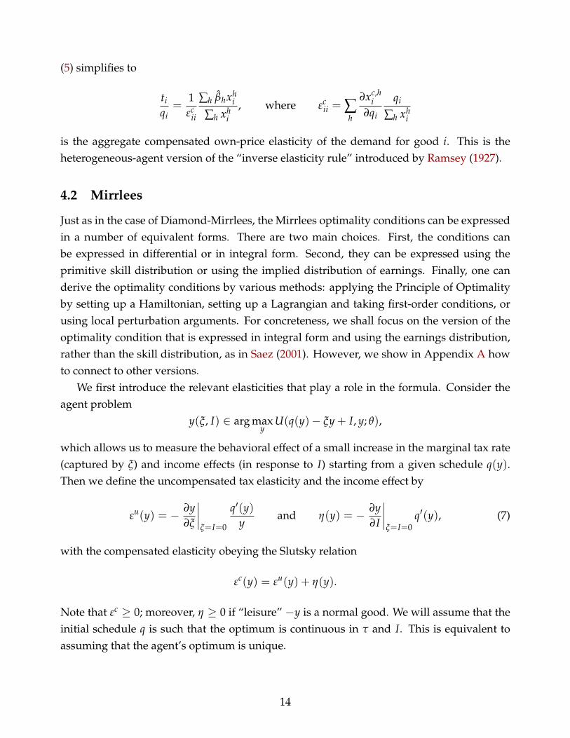
Since each agent increases y, this produces a shift in the distribution H to the right. Ata particular point (y, H(y)), the horizontal shift equals precisely t′(y)

q′(y) εc(y)y. Equation (11),however, demands the implied vertical shift. To translate the horizontal shift into the verticalshift requires multiplying by the slope of H, that is, the density h. We conclude that the left-

12Diamond (1998), however, expressed the formula as a function of the primitive skill distribution, ratherthan the implied earnings distribution.

16

Hc(y; 0)Hc(y; τ)

t′(y)q′(y) εc(y)y

t′(y)q′(y) εc(y)yh(y)

y

Figure 1: Shift in aggregate compensated demand 1− Hc(y) at y.

hand side of (5) equals

∂

∂τ(1− Hc(y; τ))

∣∣∣∣τ=0

=t′(y)q′(y)

εc(y)yh(y). (12)

This is illustrated in Figure 1. The formal derivation is contained in Appendix A.Equation (12) reveals that the left-hand side of the Diamond-Mirrlees formula simplifies

drastically when applied to the Mirrlees setting: the relevant response for y only dependson the variation in the marginal tax rate t′(y) at y, and not on the variation in the entireschedule in (10). In other words, the Mirrlees model constitutes the rare diagonal case wherecompensated cross-price elasticities of demand are zero and only the own-price elasticitymatters. This coveted case is often highlighted in the commodity tax literature for it impliesRamsey’s “inverse elasticity rule.”

5.2 Right-Hand Side in Diamond-Mirrlees

The analog, with a continuum of goods, of the right-hand side of equation (6) in conjunctionwith (5) is

∫ ∞

0(1− Hθ(y))

(βθ − 1− ∂

∂I

∫ ∞

0t′(z) (1− Hθ(z; I)) dz

)dF(θ)

=∫ ∞

θ(y)

(βθ − 1− ∂

∂I

∫ y(θ;I)

0t′(z)dz

)dF(θ)

=∫ ∞

θ(y)

(βθ − 1− t′(y(θ))

∂y(θ; I)∂I

)dF(θ), (13)

17

where θ(y) denotes the inverse of y(θ).13 Substituting ∂y(θ; I)/∂I = −η(y)/q′(y) into (13)and changing variables from θ to y = y(θ) yields

−∫ ∞

y(1− βy)dH(y) +

∫ ∞

y

t′(y)q′(y)

η(y)dH(y), (14)

with a slight abuse of notation to write βy for βθ(y).

5.3 Putting it Together

Equating (12) and (14) yields

− t′(y)q′(y)

εc(y)yh(y) =∫ ∞

y(1− βy)dH(y)−

∫ ∞

y

t′(y)q′(y)

η(y)dH(y). (15)

To translate this into the Mirrlees model with a nonlinear tax over pre-tax earnings p(y), weset q(y) = p(y)− T(p(y)) and recall that t(y) = q(y)− p(y), so that t(y) = −T(p(y)) and

t′(y)q′(y)

= − T′(p(y))1− T′(p(y))

, (16)

which upon substitution gives precisely the Mirrlees formula (8).It might seem surprising that applying the Diamond-Mirrlees formula (5) to the Mir-

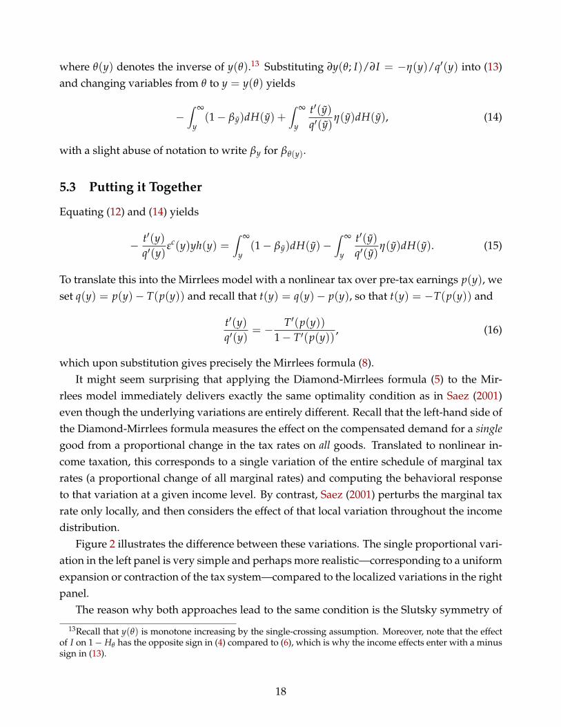
rlees model immediately delivers exactly the same optimality condition as in Saez (2001)even though the underlying variations are entirely different. Recall that the left-hand side ofthe Diamond-Mirrlees formula measures the effect on the compensated demand for a singlegood from a proportional change in the tax rates on all goods. Translated to nonlinear in-come taxation, this corresponds to a single variation of the entire schedule of marginal taxrates (a proportional change of all marginal rates) and computing the behavioral responseto that variation at a given income level. By contrast, Saez (2001) perturbs the marginal taxrate only locally, and then considers the effect of that local variation throughout the incomedistribution.

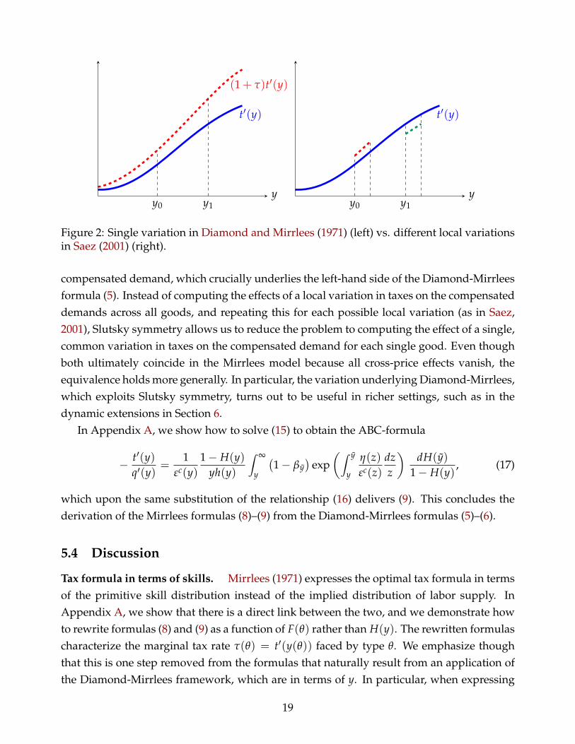
Figure 2 illustrates the difference between these variations. The single proportional vari-ation in the left panel is very simple and perhaps more realistic—corresponding to a uniformexpansion or contraction of the tax system—compared to the localized variations in the rightpanel.

The reason why both approaches lead to the same condition is the Slutsky symmetry of

13Recall that y(θ) is monotone increasing by the single-crossing assumption. Moreover, note that the effectof I on 1− Hθ has the opposite sign in (4) compared to (6), which is why the income effects enter with a minussign in (13).

18

t′(y)

(1 + τ)t′(y)

y0 y1y

t′(y)

y0 y1y

Figure 2: Single variation in Diamond and Mirrlees (1971) (left) vs. different local variationsin Saez (2001) (right).

compensated demand, which crucially underlies the left-hand side of the Diamond-Mirrleesformula (5). Instead of computing the effects of a local variation in taxes on the compensateddemands across all goods, and repeating this for each possible local variation (as in Saez,2001), Slutsky symmetry allows us to reduce the problem to computing the effect of a single,common variation in taxes on the compensated demand for each single good. Even thoughboth ultimately coincide in the Mirrlees model because all cross-price effects vanish, theequivalence holds more generally. In particular, the variation underlying Diamond-Mirrlees,which exploits Slutsky symmetry, turns out to be useful in richer settings, such as in thedynamic extensions in Section 6.

In Appendix A, we show how to solve (15) to obtain the ABC-formula

− t′(y)q′(y)

=1

εc(y)1− H(y)

yh(y)

∫ ∞

y

(1− βy

)exp

(∫ y

y

η(z)εc(z)

dzz

)dH(y)

1− H(y), (17)

which upon the same substitution of the relationship (16) delivers (9). This concludes thederivation of the Mirrlees formulas (8)–(9) from the Diamond-Mirrlees formulas (5)–(6).

5.4 Discussion

Tax formula in terms of skills. Mirrlees (1971) expresses the optimal tax formula in termsof the primitive skill distribution instead of the implied distribution of labor supply. InAppendix A, we show that there is a direct link between the two, and we demonstrate howto rewrite formulas (8) and (9) as a function of F(θ) rather than H(y). The rewritten formulascharacterize the marginal tax rate τ(θ) = t′(y(θ)) faced by type θ. We emphasize thoughthat this is one step removed from the formulas that naturally result from an application ofthe Diamond-Mirrlees framework, which are in terms of y. In particular, when expressing

19

them in terms of elasticities, the formulas in terms of θ require the use of different elasticityconcepts in general.14

Technology and tax instruments. An advantage of deriving the Mirrlees optimal tax for-mula from the Diamond-Mirrlees formula is that it allows for a general structure of theproduction side of the economy. A general, possibly nonlinear, production function is a keyfeature of the Diamond-Mirrlees model. In contrast, the baseline Mirrlees setup involves asimple linear technology. As our derivation makes clear, the Mirrlees formula for the opti-mal nonlinear income tax schedule holds for any production function G(H). In other words,based on our connection, the result of Diamond and Mirrlees (1971) that their tax formula isindependent of technology now applies to the Mirrlees model.

Our specification of technology matters for this result. In particular, with G(H), out-put only depends on the distribution of effective labor in the economy, consistent with theproduction function in Diamond and Mirrlees (1971). Alternative specifications may affectthe analysis. Consider, for instance, a two-sector economy with technology G(H1, H2), soa given level of labor supply y can have different effects depending on whether it enters insector 1 or 2. In this case, the Diamond-Mirrlees framework continues to apply, and henceour analysis carries over, as long as sector-specific tax schedules t1(y) and t2(y) are avail-able. In the absence of this, with only a single tax schedule t(y), the Mirrlees formula wouldneed to be modified to reflect general equilibrium effects on redistribution (Stiglitz, 1982,and Rothschild and Scheuer, 2013).15 Moreover, production efficiency would not necessar-ily be optimal with restricted tax instruments (Guesnerie, 1998, Naito, 1999, and Scheuer,2014).16

Under our specification of technology, however, none of these considerations play a role:A single non-linear income tax schedule is sufficient and the corresponding optimal tax for-mula is independent of the shape of G.

Multiple consumption goods. In line with the original Mirrlees model, we have consid-ered a single consumption good. Since the Diamond-Mirrlees model naturally allows forany number of commodities, it is straightforward, however, to extend our analysis to multi-

14It is also possible to rewrite the optimal tax formulas as a function of the implied distribution of earningsp(y), again requiring different elasticity concepts in general when p(y) 6= y (see for example Scheuer andWerning (2015) for the required elasticity adjustments in the context of superstar effects).

15Rothschild and Scheuer (2014) provide an extension to N ≥ 2 sectors and a more general technology(allowing for externalities). Ales et al. (2015) and Sachs et al. (2016) consider models where each type θ corre-sponds to a separate sector, the former with a discrete set of types/sectors and the latter with a continuum.

16Saez (2004) links a discrete jobs model to the Diamond-Mirrlees model and discusses the implications ofnonlinear production functions, also contrasting the results with Stiglitz (1982) and Naito (1999). However,Saez (2004) does not attempt to derive the Mirrlees optimal tax formula.

20

ple consumption goods. With linear taxes on each of the consumption goods (normalizingone of them to zero), an application of conditions (5) and (6) would immediately deliver for-mulas for (i) the optimal linear commodity tax rates in the presence of the optimal nonlinearlabor income tax schedule and (ii) marginal tax rates of the optimal nonlinear income taxschedule in the presence of the optimal commodity taxes.

Such formulas have been derived in the literature using standard mechanism design (seefor example Mirrlees, 1976, and Jacobs and Boadway, 2014) or variational approaches (e.g.Christiansen, 1984, and Saez, 2002a). A crucial feature of these formulas are conditional laborelasticities of the commodity demands, which measure how the demand for a consumptiongood ci changes when labor y changes but after-tax income q(y) is held fixed. When thesecross-elasticities are zero, which holds under the weakly separable preference specificationU(u(c1, ..., cN), y; θ) considered by Atkinson and Stiglitz (1976), it then immediately followsthat (i) all commodity taxes are zero at the optimum, and (ii) the formula for the optimalmarginal income tax rates is the same as derived here.

6 Four Extensions of the Mirrlees Model

In this section, we briefly consider four extensions that illustrate the power and ease of ourapproach. First, we extend the Mirrlees model to a lifecycle framework where workers payan annual income tax, but productivity varies from year to year. Second, we incorporate hu-man capital investments into this lifecycle framework, endogenizing individuals’ lifetimeproductivity profiles. Third, we enrich the static Mirrlees model to allow for additionalarbitrary dimensions of heterogeneity, without single-crossing assumptions. Fourth, we in-corporate an extensive margin, alongside the intensive margin, for labor supply. The firsttwo of these extensions are novel, and would be rather cumbersome to tackle with the usualmechanism design approach. The third and fourth extensions of the Mirrlees models haveprecedents in the existing literature.17 While our assumptions and results are slightly differ-ent, the main benefit of our treatment of these extensions is to illustrate the power and easeof our approach based on the Diamond-Mirrlees formula.

6.1 Annual Taxation of Earnings in a Lifecycle Context

The original Mirrlees model is a one-shot static model: there is a single consumption goodand a single labor supply choice. We now consider a simple dynamic extension, to incorpo-

17See, among others, Saez (2001), Hendren (2014) and Jacquet and Lehmann (2015) for the third and Dia-mond (1980), Saez (2002b), Choné and Laroque (2011), Jacquet et al. (2013), Zoutman et al. (2013) and Hendren(2014) for the fourth extension.

21

rate a lifecycle choice for labor supply.

Setup. Suppose ex ante heterogeneity is indexed by θ ∼ F(θ) as before. Each individualfaces varying productivities δ over her lifetime with conditional distribution P(δ|θ). Indi-viduals choose how much labor to supply for each δ, resulting in a schedule y(δ; θ). Thegovernment sets a nonlinear income tax schedule, resulting in the retention function q(y)for the income earned at any point in time (i.e. an “annual” tax without age- or history-dependence, as is the case in practice). Moreover, markets are complete, so individualssmooth consumption over their lifecycle respecting their budget constraint

c =∫ ∞

0q(y(δ; θ))dP(δ|θ).

Preferences areU(c, Y; θ)

withY =

∫ ∞

0v(y(δ; θ), δ)dP(δ|θ).

Here, v(y, δ) is a measure of the instantaneous disutility from supplying effective labor y ata moment when productivity is δ; as usual we assume v satisfies single-crossing in δ. ThenY captures the total disutility from labor over the individual’s lifetime. We do not requireassumptions about the nature of ex ante heterogeneity in θ.

Formula for the optimal annual tax. As before, we can think of each individual as choos-ing a distribution Hθ(y) over y. The only difference is that this distribution is no longerdegenerate (i.e., no longer a step function). Using this insight, we show in Appendix B thatour analysis carries over easily and leads to the following formula for the optimal annualtax t(y):

− yεF(y)h(y)(

t′(y)q′(y)

+ Λ(y))=∫ ∞

y

(1− βy

)dH(y)−

∫ ∞

yη(y)

t′(y)q′(y)

dH(y). (18)

This is very similar to the static formula (15) except for the following differences.First, on the right-hand side, η(y) is the average income effect and βy the average social

welfare weight at y (across θ).Second, εF(y) ≥ 0 is a Frisch elasticity of labor supply that holds fixed λ ≡ −Uc/UY, i.e.

the marginal rate of substitution between lifetime consumption and lifetime labor supply.This Frisch elasticity is purely local in the sense that it depends only on the local shape ofthe flow disutility function v and on the local shape of the annual tax schedule at y.

22

Third, there is an extra term on the left-hand side

Λ(y) =∫

Θ

1λc(τ, θ)

∂λc(τ, θ)

∂τ

∣∣∣∣τ=0

dF(θ|y), (19)

which captures precisely the lifetime effects on the compensated labor supply. In particular(and as explained in more detail in Appendix B), λc(τ, θ, ; U) is defined such that

yF(τ, λc(τ, θ; U)) = yc(τ, θ; U),

where yF is the Frisch labor supply, holding λ fixed, and yc is the compensated labor supply,holding lifetime utility U fixed (we dropped the argument U in λc). This captures globaleffects on labor supply and the interactions of labor supply across different “ages,” i.e. acrossdifferent values of δ. The effect Λ(y) will generally depend on the entire tax schedule.

Lifetime effects. To illustrate the mechanics underlying the lifetime effects Λ, considerlifetime preferences of the additively separable form

U(

u(c)−∫ ∞

0v(y(δ; θ), δ)dP(δ|θ); θ

).

We show in Appendix B that, in this case,

1λc(τ, θ)

∂λc(τ, θ)

∂τ

∣∣∣∣τ=0

= u′′(c(θ))

∫ ∞0 t′(y)yεF(y)dH(y|θ)

u′(c(θ))− u′′(c(θ))∫ ∞

0 q′(y)yεF(y)dH(y|θ).

Hence, the lifetime effects depend on the entire tax schedule, Frisch elasticities throughoutthe income distribution, and risk aversion. Notably, under the standard conditions that u(c)is concave and marginal income tax rates T′(p(y)) are positive (so t′(y) ≤ 0 by (16)), wehave Λ(y) > 0.

Intuitively, the marginal rate of substitution between lifetime consumption and lifetimelabor supply is simply λ = u′(c), and a proportional increase in all marginal tax rates re-duces lifetime consumption and therefore increases marginal utility of consumption. Similarto income effects, this provides a force for higher marginal tax rates. On the other hand, itis straightforward to show (see Appendix B) that the Frisch elasticity, as usual in lifecyclesettings, exceeds the compensated labor supply elasticity: εF(y) ≥ εc(y, θ) for all θ, y. Thisprovides a force in the opposite direction.

In the case of the quasilinear lifetime preferences with u(c) = c, the lifetime effects Λvanish and the elasticities coincide. Hence, in this case, the standard formula from the static

23

setting fully extends to the annual tax in this much richer lifecycle framework.18

Welfare weights. Even though the formula for the optimal annual tax in our dynamic set-ting coincides in structure with the formula for the static case, the lifecycle framework hasimportant implications for the average welfare weights βy at a given income y on the right-hand side of (18). The fundamental welfare weights βθ only vary with ex ante (i.e., lifetime)heterogeneity θ. Since there can be substantially less lifetime inequality than cross-sectionalinequality at any given point in time (which is driven by δ in addition to θ), the averagewelfare weights at a given income βy naturally vary less than in the static framework. Anextreme case occurs when there is no ex ante heterogeneity, so all income inequality is drivenby the shocks δ. When viewed over their entire lifetimes, all individuals face the same dis-tribution of these shocks, but the resulting cross-sectional income inequality at any point intime can be arbitrarily large. In this case, βy is independent of y and optimal annual taxesare zero.

6.2 Human Capital

It is easy to incorporate human capital investment in this lifecycle framework. In particular,suppose individuals choose an education level e before entering the labor market, whichaffects their productivity distribution P(δ|θ, e). Their lifetime utility is U(c, Y; θ, e), whichcan capture costs of the education investment e in a general form (and note that these costscan differ across θ-types). Otherwise, the framework is identical to the one in the precedingsubsection. As before, the government looks for the optimal annual nonlinear income taxschedule, or equivalently q(y).19

As we show in Appendix B, all the results from the basic lifecycle framework go through.In particular, the optimal tax formula (18) still applies. The effect Λ(y) takes the same formas before (given by (19)), but now also captures the effect of taxes on individuals’ humancapital choices. The term Λ again vanishes if lifetime preferences take the quasilinear formU(c, Y; θ, e) = U(c−Y; θ, e). More generally, the extra term can be interpreted as a ”catch all”

18Farhi and Werning (2013) compute these restricted taxes numerically. Assuming quasilinear and iso-elasticpreferences, Golosov et al. (2014) use their general variational approach to provide a formula for the welfareeffects of an age- and history-independent reform of the nonlinear labor tax schedule. Their formula featuresa weighted average of parameters of the age-specific labor income distributions, age-specific labor elasticities,and age-specific cross-effects on capital tax revenue (which we abstract from). Their focus is on comparing thisto an age-dependent reform. Our formula based on Diamond and Mirrlees (1971) holds for general preferencesand only relies on the cross-sectional income distribution, highlighting the similarity to the static case.

19We abstract from exploring the optimal tax treatment of the human capital investment e by assuming thatit is not taxed nor subsidized directly (see e.g. Bovenberg and Jacobs, 2005, and Stantcheva, 2016, for recentwork on this issue).

24

for any additional margins that affect individuals’ lifetime productivity profiles and budgetconstraints.

6.3 More General Forms of Heterogeneity

An important advantage of approaching the Mirrlees model from the perspective of theDiamond-Mirrlees framework is that we can easily accommodate relatively general forms ofheterogeneity, as we now show. General forms of heterogeneity are inherent to the structurein Diamond-Mirrlees. In contrast, the baseline Mirrlees setup allows for only one dimensionof heterogeneity satisfying a single-crossing condition.

Returning to the static framework, suppose there are groups, indexed by φ and dis-tributed according to c.d.f. P(φ) (and support Φ) in the population, with preferences

U(c, y; θ, φ).

We only require that the single-crossing property in terms of θ is satisfied among individualswith the same φ, i.e. MRS(c, y; θ, φ) is strictly decreasing in θ for each φ. Apart from that,we can allow for arbitrary preference heterogeneity captured by φ. For example, φ couldbe from a finite set or a continuum, and it could be single- or multidimensional. This isin line with the Diamond-Mirrlees model, where h can index arbitrary differences acrosshouseholds.

In Appendix B, we show how to generalize the analysis from Section 5 to such a frame-work. The Mirrlees optimal tax formulas (8) and (9) go through when replacing the elas-ticities εc(y) and η(y) as well as the marginal social welfare weights βy by their averagesconditional on y. For example, εc(y) is simply replaced by

εc(y) = E[εc(y, φ)|y] =∫

Φεc(y, φ)dP(φ|y),

where P(φ|y) is the distribution of φ conditional on y (and analogously for η(y) and βy).20

20Using his perturbation approach, Saez (2001) derives this result for the asymptotic top marginal tax rate.Hendren (2014) provides a formula for the fiscal externality from changes to the nonlinear income tax schedulethat depends on average elasticities at each income level, also based on a perturbation approach. Jacquet andLehmann (2015) consider the same structure of heterogeneity as here and obtain this result for the optimal taxformula for the special case of additively separable preferences based on both an extended mechanism designapproach with pooling and perturbation arguments.

25

6.4 Extensive-Margin Choices

Finally, we demonstrate how the Diamond-Mirrlees setting can easily incorporate extensivemargin labor choices, generalizing the environments considered by Diamond (1980), Saez(2002b), Choné and Laroque (2011), and Jacquet et al. (2013) among others. We shall derivethe resulting tax formula starting from the Diamond-Mirrlees formulas (5)–(6).

For simplicity, suppose individuals are characterized by two-dimensional heterogeneity(θ, ϕ) with preferences

V(c, y; θ, ϕ) =

{U(c, y; θ) if y > 0u(c; θ, ϕ) if y = 0.

Hence, heterogeneity in the ϕ-dimension only drives participation decisions but not inten-sive margin decisions conditional on θ.21 In other words, preferences are the same as inSection 5 for strictly positive y but can exhibit a discontinuity at y = 0 that can be differentacross individuals with the same θ. Assuming that u is increasing in ϕ, this will lead indi-viduals with high values of ϕ, for any given θ, to stay out of the labor market and choosey = 0, consuming the demogrand q(0).

We show in Appendix B that an application of the Diamond-Mirrlees formulas in thiscase leads to the following simple modification of formula (8):

T′(y)1− T′(y)

εc(y)yh(y) =∫ ∞

y

(1− βy +

T′(y)1− T′(y)

η(y)− T(y)− T(0)q(y)− q(0)

ρ(y))

dH(y), (20)

where ρ(y) is the participation elasticity at y, defined by

ρ(y) =∂h(y)

∂(q(y)− q(0))q(y)− q(0)

h(y)

∣∣∣∣{y(θ)}

,

which is the percentage change in the density at y when the participation incentives mea-sured by q(y)− q(0) are increased by one percent, holding fixed the intensive margin choicesof all individuals with y > 0 (i.e. holding fixed the y(θ)-schedule). Moreover, βy is the aver-age social welfare weight on individuals who choose y.

As in the lifecycle extensions, the (compensated) demand system is no longer diagonalwith an active extensive margin: The proportional change in all marginal tax rates underly-ing the left-hand side of (5) affects 1− H(y) not just through the (compensated) intensive-margin response at y, but also through the (compensated) extensive-margin responses of all

21Such further heterogeneity could be easily incorporated as shown in the previous subsection. We focus onthe extensive margin here.

26

individuals with labor supply above y. Combining this with the pure income effect on theextensive margin from (6) leads to the additional term on the right-hand side of the optimaltax formula.22

A special case arises when only the extensive margin is active (see e.g. Diamond, 1980,and Choné and Laroque, 2011), in which case (20) reduces to

T(y)− T(0)q(y)− q(0)

=1− βy

ρ(y),

i.e., an inverse elasticity rule similar to the pure intensive margin model considered so far,but in terms of the average tax rate and the participation elasticity.

7 Conclusion

This paper uncovered a deep connection between two canonical models in public financeand their optimal tax formulas. We find this connection is insightful and, thus, worthwhilein its own right. In addition, this line of attack on the nonlinear tax problem can easily allowfor weaker conditions and extensions. We have provided four such extensions to illustratethe appeal of the Diamond-Mirrlees approach. We conjecture that this approach could beusefully applied in other settings as well.

References

Ales, L., M. Kurnaz, and C. Sleet, “Tasks, Talents, and Taxes,” American Economic Review,2015, 105, 3061–3101. 15

Atkinson, A. and J. Stiglitz, “The Design of Tax Structure: Direct Versus Indirect Taxation,”Journal of Public Economics, 1976, 6, 55–75. 5.4

Bovenberg, L. and B. Jacobs, “Redistribution and Education Subsidies are Siamese Twins,”Journal of Public Economics, 2005, 89, 2005–2035. 19

Brown, S. and D. Sibley, The Theory of Public Utility Pricing, Cambridge University Press,1986. 522Saez (2002b) derives the equivalent of this formula for a discrete type setting and for the special case with-

out income effects using a perturbation approach (the working paper version in Saez (2000) also provides acontinuous types analogue). Jacquet et al. (2013) consider preferences with an additively separable partici-pation cost (so V(c, y; θ, ϕ) = U(c, y; θ) − I(y > 0)ϕ). For this special case of our environment, they derivethe same formula as ours using perturbation and mechanism design approaches. Zoutman et al. (2013) andHendren (2014) provide related formulas for the fiscal externality in the inverse optimum problem with bothintensive and extensive margins.

27

Chamley, C., “Optimal Taxation of Capital Income in General Equilibrium with InfiniteLives,” Econometrica, 1986, 54, 607–622. 1

Choné, P. and G. Laroque, “Optimal Taxation in the Extensive Model,” Journal of EconomicTheory, 2011, 146, 425–453. 17, 6.4, 6.4

Christiansen, V., “Which Commodity Taxes Should Supplement the Income Tax,” Journal ofPublic Economics, 1984, 24, 195–220. 5.4

Diamond, P., “A Many-Person Ramsey Tax Rule,” Journal of Public Economics, 1975, 4, 335–342. 1, 1, 4.1

, “Income Taxation With Fixed Hours of Work,” Journal of Public Economics, 1980, 13, 101–110. 1, 17, 6.4, 6.4

, “Optimal Income Taxation: An Example with a U-Shaped Pattern of Optimal MarginalTax Rates,” American Economic Review, 1998, 88 (1), 83–95. 1, 4.2, 12

and J. Mirrlees, “Optimal Taxation and Public Production II: Tax Rules,” American Eco-nomic Review, June 1971, 61 (3), 261–78. 1, 2, 1, 2, 2.1, 2.2, 2, 5.4, 18

Dixit, A., “The Welfare Effects of Tax and Price Changes,” Journal of Public Economics, 1975,4, 103–123. 1

Farhi, E. and I. Werning, “Insurance and Taxation over the Life Cycle,” Review of EconomicStudies, 2013, 810, 596–635. 3, 18

Goldman, B., H. Leland, and D. Sibley, “Optimal Nonuniform Prices,” Review of EconomicStudies, 1984, 51, 305–319. 1

Golosov, M., A. Tsyvinski, and N. Werquin, “A Variational Approach to the Analysis of TaxSystems,” NBER Working Paper 20780, 2014. 1, 10, 18

Guesnerie, R., “Peut-on Toujours Redistribuer les Gains a la Spécialization et à l’Echange?Un Retour Pointillé sur Ricardo et Heckscher-Ohlin,” Revue Economique, 1998, 49, 555–579.5.4

Hendren, N., “The Inequality Deflator: Interpersonal Comparisons Without a Social WelfareFunction,” NBER Working Paper 20351, 2014. 17, 20, 22

Jacobs, B. and R. Boadway, “Optimal Linear Commodity Taxation Under Optimal Non-linear Income Taxation,” Journal of Public Economics, 2014, 117, 201–210. 5.4

28

Jacquet, L. and E. Lehmann, “Optimal Income Taxation when Skills and Behavioral Elastic-ities are Heterogeneous,” CESifo Working Paper 5265, 2015. 1, 4.2, 17, 20

, , and B. Van der Linden, “The Optimal Marginal Tax Rates with both Extensive andIntensive Responses,” Journal of Economic Theory, 2013, 148, 1770–1805. 1, 17, 6.4, 22

Judd, K., “Redistributive taxation in a simple perfect foresight model,” Journal of Public Eco-nomics, 1985, 28, 59–83. 1

Mirrlees, J., “An Exploration in the Theory of Optimum Income Taxation,” Review of Eco-nomic Studies, 1971, 38, 175–208. 1, 1, 2, 2.2, 5.4

, “Optimal Commodity Taxation in a Two-Class Economy,” Journal of Public Economics,1975, 4, 27–33. 1

, “Optimal Tax Theory: A Synthesis,” Journal of Public Economics, 1976, 6, 327–358. 4.1, 5.4

Naito, H., “Re-Examination of Uniform Commodity Taxes Under a Non-linear Income Taxand its Implication for Production Efficiency,” Journal of Public Economics, 1999, 71 (165-188). 5.4, 16

Piketty, T., “La Redistribution Fiscale Face au Chômage,” Revue française d’économie, 1997,12, 157–201. 1, 4, 1

Ramsey, F., “A Contribution to the Theory of Taxation,” Economic Journal, 1927, 37, 47–61.4.1

Roberts, K., “A Reconsideration of the Optimal Income Tax,” in P. Hammond and G. Myles,eds., Incentives and Organization: Papers in Honour of Sir James Mirrlees, Oxford UniversityPress, 2000. 1, 4.2

Rothschild, C. and F. Scheuer, “Redistributive Taxation in the Roy Model,” Quarterly Journalof Economics, 2013, 128, 623–668. 5.4

and , “A Theory of Income Taxation under Multidimensional Skill Heterogeneity,”Working Paper, 2014. 15

Sachs, D., A. Tsyvinski, and N. Werquin, “Non-Linear Tax Incidence and Optimal Taxationin General Equilibrium,” Mimeo, 2016. 15

Saez, E., “Optimal Income Transfer Programs: Intensive versus Extensive Labor SupplyResponses,” NBER Working Paper 7708, 2000. 22

29

, “Using Elasticities to Derive Optimal Income Tax Rates,” Review of Economic Studies, 2001,68 (1), 205–29. 1, 1, 4.2, 4.2, 5.3, 2, 5.3, 17, 20

, “The Desirability of Commodity Taxation under Non-linear Income Taxation and Het-erogeneous Tastes,” Journal of Public Economics, 2002, 83, 217–230. 5.4

, “Optimal Income Transfer Programs: Intensive versus Extensive Labor Supply Re-sponses,” The Quarterly Journal of Economics, 2002, 117 (3), 1039–1073. 1, 1, 17, 6.4, 22

, “Direct Or Indirect Tax Instruments For Redistribution: Short-Run Versus Long-Run,”Journal of Public Economics, 2004, 88, 503–518. 16

Scheuer, F., “Entrepreneurial Taxation with Endogenous Entry,” American Economic Journal:Economic Policy, 2014, 6, 126–163. 5.4

and I. Werning, “The Taxation of Superstars,” Quarterly Journal of Economics, 2015, forth-coming. 4.2, 14

Stantcheva, S., “Optimal Taxation and Human Capital Policies over the Life Cycle,” Mimeo,Harvard University, 2016. 19

Stiglitz, J., “Self-Selection and Pareto Efficient Taxation,” Journal of Public Economics, 1982,17, 213–240. 5.4, 16

Tirole, Jean, The Theory of Industrial Organization, MIT Press, 2002. 5

Weinzierl, M., “The Surprising Power of Age-Dependent Taxes,” Review of Economic Studies,2011, 78, 1490–1518. 3

Zoutman, F., B. Jacobs, and E. Jongen, “Revealed Social Preferences of Dutch Political Par-ties,” Working Paper, 2013. 17, 22

A Derivations

A.1 Derivation of Equation (12)

The the left-hand side of (5) with a continuum of goods equals

∂

∂τ

∫ ∞

0(1− Hc

θ(y; τ))dF(θ)∣∣∣∣τ=0

=∂

∂τ

∫ ∞

θc(y;τ)dF(θ)

∣∣∣∣τ=0

= − ∂θc(y; τ)

∂τ

∣∣∣∣τ=0

f (θ(y)) (21)

30

where the superscript c indicates compensated choices, θ(y; τ) is the inverse of y(θ; τ) withrespect to its first argument, and θ(y) stands short for θ(y; 0). We are using the fact thaty(θ; τ) is increasing in θ for any τ by the single-crossing condition.

The optimum for agent θ must satisfy the tangency condition

MRS(c, y; θ) = q′(y; τ) = q′(y) + τt′(y). (22)

To compute the compensated demand, we use this equation with c = e(v, y; θ) where e is theinverse of U with respect to its first argument. To compute the uncompensated demand, weuse the budget constraint c = q(y) + I. Differentiating (22) yields

∂θc(y; τ)

∂τ

∣∣∣∣τ=0

=q′(y)− p′(y)

MRSθ=

t′(y)/q′(y)MRSθ/MRS

. (23)

Moreover, observe that the density of y is given by h(y) = f (θ(y))θ′(y). Again differentiat-ing (22) for τ = 0 yields

θ′(y) = −MRSc +

MRSyMRS −

q′′q′

MRSθ/MRS. (24)

Finally, the elasticities defined in (7) can be obtained by differentiating

MRS(q(y)− ξy + I, y; θ) = q′(y)− ξ.

Hence,

εu(y) =−MRSc + 1/y

MRSc +MRSyMRS −

q′′q′

, (25)

η(y) =MRSc

MRSc +MRSyMRS −

q′′q′

, (26)

andεc(y) = εu(y) + η(y) =

1/y

MRSc +MRSyMRS −

q′′q′

. (27)

Using (27) in (24) yields

θ′(y) = − 1yεc(y)

1MRSθ/MRS

. (28)

Substituting all this in (21), we obtain (12).

31

A.2 Derivation of Equation (17)

Defineµ(y) ≡ − t′(y)

q′(y)εc(y)yh(y)

and write equation (15) as

µ(y) =∫ ∞

y(1− βy)dH(y) +

∫ ∞

y

η(y)εc(y)

µ(y)y

dy.

Differentiating this yields

µ′(y) + (1− βy)h(y) = −η(y)εc(y)

µ(y)y

.

Integrating this ordinary first-order differential equation forward to solve for µ yields (17).

A.3 Formulas in Terms of the Skill Distribution

Combine (21) and (23) and change variables from θ to y(θ) to write the left-hand side of (5)as

t′(y(θ))/q′(y(θ))MRSθ/MRS

f (θ) =τ(θ)

1− τ(θ)θ f (θ)χ(θ),

where we defined τ(θ) = T′(p(y(θ))) and χ(θ) = − (MRSθθ/MRS)−1. Using this togetherwith (14) yields

τ(θ)

1− τ(θ)θ f (θ)χ(θ) =

∫ ∞

θ(1− βθ)dF(θ) +

∫ ∞

θ

τ(θ)

1− τ(θ)η(θ)dF(θ), (29)

where we slightly abused notation to write η(θ) = η(y(θ)). This is the equivalent of (8)written in terms of θ. Defining the left-hand side of equation (29) as µ(θ), we can write it as

µ(θ) =∫ ∞

θ(1− βθ)dF(θ) +

∫ ∞

θ

η(θ)

θχ(θ)µ(θ)dθ.

Observe thatη(θ)

θχ(θ)=

η(θ)

εc(θ)

y′(θ)y(θ)

,

where we used (26), (27) and (28) (and, again slightly abusing notation, wrote εc(θ) =

εc(y(θ))). Using this and differentiating yields

µ′(θ) + (1− βθ) f (θ) = − η(θ)

εc(θ)

y′(θ)y(θ)

µ(θ).

32

Solving this forward yields

τ(θ)

1− τ(θ)=

1χ(θ)

1− F(θ)θ f (θ)

∫ ∞

θ(1− βθ) exp

(∫ θ

θ

η(s)εc(s)

dy(s)y(s)

)dF(θ)

1− F(θ), (30)

which is the equivalent of (9) written in terms of θ.

B Extensions

B.1 Lifecycle Framework

Derivation of formula (18). Due to single-crossing in δ, y(δ; θ) is increasing in δ, so

1− Hθ(y) =∫ ∞

0(1− Hδ,θ(y))dP(δ|θ)

where1− Hδ,θ(y) = I(y ≤ y(δ; θ)).

Hence, the left-hand side of (5) simply becomes

∂

∂τ(1− Hc(y; τ))

∣∣∣∣τ=0

=∂

∂τ

∫Θ(1− Hc

θ(y; τ))dF(θ)∣∣∣∣τ=0

=∂

∂τ

∫Θ

∫ ∞

0(1− Hc

δ,θ(y; τ))dP(δ|θ)dF(θ)∣∣∣∣τ=0

=∂

∂τ

∫Θ

∫ ∞

δc(y;θ,τ)dP(δ|θ)dF(θ)

∣∣∣∣τ=0

= −∫

Θp(δ(y; θ)|θ) ∂δc(y; θ, τ)

∂τ

∣∣∣∣τ=0

dF(θ) (31)

where δ(y; θ) is the inverse of y(δ; θ) with respect to its first argument and p(δ|θ) is thedensity corresponding to P(δ|θ).

Individuals solve

maxc(θ),y(δ;θ)

U(

c(θ),∫ ∞

0v(y(δ; θ), δ)dP(δ|θ); θ

)subject to

c(θ) =∫ ∞

0q(y(δ; θ))dP(δ|θ)

33

with first-order conditions

Uc = λ

UYvy(y(δ; θ), δ) = −λq′(y(δ; θ)).

The Frisch labor supply as defined in the main text is thus yF(δ; λ, τ) such that

vy(yF, δ) = λq′(yF; τ)

where λ ≡ −λ/UY. Note that λ will in general depend on θ.We can write the compensated labor supply as yc(δ; θ, U, τ) such that

vy(yc, δ) = λc(θ, U, τ)q′(yc; τ).

Dropping the argument U, this equivalently determines δc(y; θ, τ) such that

vy(y, δc) = λc(θ, τ)q′(y; τ).

We are now able to compute

∂δc(y; θ, τ)

∂τ

∣∣∣∣τ=0

=∂λc

∂τ q′ + λct′

vyδ=

1λc

∂λc

∂τ + t′/q′

vyδ/vy.

At τ = 0, we can also compute (for the change of variables from δ to y)

∂δ(y; θ)

∂y≡ δ′(y; θ) = −

vyy − λcq′′

vyδ= −

vyy/vy − q′′/q′

vyδ/vy.

Finally, note that the Frisch elasticity is based on

vy(yF, δ) = λ(

q′(yF)− ξ)

,

so

εF(y) = − ∂yF

∂ξ

∣∣∣∣ξ=0

q′

y=

λ

vyy − λq′′q′

y=

1/yvyy/vy − q′′/q′

. (32)

(Observe that this does not depend on θ and that the denominator must be non-negative by

34

the second-order condition.) Using all this, we can write (31) as

∫Θ

p(δ(y; θ)|θ)δ′(y; θ)1λc

∂λc

∂τ + t′/q′

vyy/vy − q′′/q′dF(θ)

=∫

Θp(δ(y; θ)|θ)δ′(y; θ)

(1λc

∂λc

∂τ+ t′/q′

)yεF(y)dF(θ)

= yεF(y)h(y)(

t′(y)q′(y)

+∫

Θ

1λc

∂λc

∂τdF(θ|y)

).

For the last step, we noted that λc(θ, τ) depends on θ and we used the fact that

p(δ(y; θ)|θ)δ′(y; θ) f (θ)h(y)

= f (θ|y). (33)

To see this, note that, given θ, by monotonicity of δ in y, we have H(y|θ) = P(δ(y; θ)|θ). Dif-ferentiating this, we obtain the density of y conditional on θ: h(y|θ) = p(δ(y; θ)|θ)δ′(y; θ).Multiplying this by the marginal density f (θ) for θ, we obtain the joint density h(y, θ) =

p(δ(y; θ)|θ)δ′(y; θ) f (θ). By Bayes’ Rule, this implies the conditional density f (θ|y) of θ con-ditional on y given by (33).

As for the right-hand side, we have

∫Θ

∫ ∞

0(1− Hδ,θ(y))

(βθ − 1− ∂

∂I

∫ ∞

0t′(z) (1− Hδ,θ(z; I)) dz

)dP(δ|θ)dF(θ)

=∫

Θ

∫ ∞

δ(y;θ)

(βθ − 1− ∂

∂I

∫ y(δ;θ,I)

0t′(z)dz

)dP(δ|θ)dF(θ)

=∫

Θ

∫ ∞

δ(y;θ)

(βθ − 1− ∂y(δ; θ, I)

∂It′(y(δ; θ))

)dP(δ|θ)dF(θ).

Using ∂y(δ(y; θ); θ, I)/∂I = −η(y, θ)/q′(y), this becomes after changing variables in theinner integral

∫Θ

∫ ∞

y

(βθ − 1 + η(z, θ)

t′(z)q′(z)

)p(δ(z; θ)|θ)δ′(z; θ)dzdF(θ)

= −∫ ∞

y

∫Θ(1− βθ) dF(θ|z)dH(z) +

∫ ∞

y

∫Θ

η(z, θ)dF(θ|z) t′(z)q′(z)

dH(z)

= −∫ ∞

y

(1− βz

)dH(z) +

∫ ∞

yη(z)

t′(z)q′(z)

dH(z), (34)

where η(y) is the average income effect and βy the average social welfare weight at y.

35

Characterizing the lifecycle effect Λ. With the separable preferences assumed in the text,we have λ = u′(c). Our goal is thus to compute the compensated effect of τ on c. To thatend, consider the compensated demand system in the dynamic framework, which solves

maxc(θ),y(δ;θ)

∫ ∞

0q(y(δ; θ); τ)dP(δ|θ)− c(θ)

subject to

u(c(θ))−∫ ∞

0v(y(δ; θ), δ)dP(δ|θ) = U(θ),

where q′(y; τ) = q′(y) + τt′(y).The compensated effects of τ on the solutions cc(θ, τ) and yc(δ; θ, τ) are therefore implic-

itly determined by the first-order conditions

vy(yc(δ; θ, τ), δ) = u′(cc(θ, τ))q′(yc(δ; θ, τ); τ)

andu(cc(θ, τ))−

∫ ∞

0v(yc(δ; θ, τ), δ)dP(δ|θ) = U(θ)

for all δ, θ, τ. Differentiating these conditions with respect to τ yields (simplifying notationand changing variables from δ to y)

∂cc(θ, τ)

∂τ

∣∣∣∣τ=0

=

∫ ∞0 t′(y)

(vyyvy− q′′

q′

)−1dH(y|θ)

1− u′′(c(θ))u′(c(θ))

∫ ∞0 q′(y)

(vyyvy− q′′

q′

)−1dH(y|θ)

.

Using the definition of the Frisch elasticity in (32), we can compute

1λc(θ)

∂λc(θ, τ)

∂τ

∣∣∣∣τ=0

=u′′(c(θ))u′(c(θ))

∂cc(θ, τ)

∂τ

∣∣∣∣τ=0

= u′′(c(θ))

∫ ∞0 t′(y)yεF(y)dH(y|θ)

u′(c(θ))− u′′(c(θ))∫ ∞

0 q′(y)yεF(y)dH(y|θ). (35)

Frisch versus compensated elasticities. Consider again the compensated demand systemsolving

maxc(θ),y(δ;θ)

∫ ∞

0(q(y(δ; θ))− ξy(δ; θ))dP(δ|θ)− c(θ)

subject to

u(c(θ))−∫ ∞

0v(y(δ; θ), δ)dP(δ|θ) = U(θ),

36

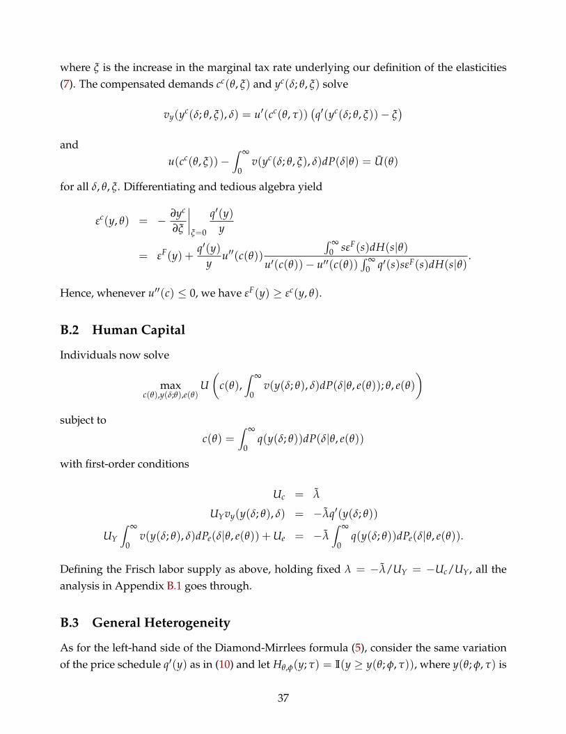
where ξ is the increase in the marginal tax rate underlying our definition of the elasticities(7). The compensated demands cc(θ, ξ) and yc(δ; θ, ξ) solve

vy(yc(δ; θ, ξ), δ) = u′(cc(θ, τ))(q′(yc(δ; θ, ξ))− ξ

)and

u(cc(θ, ξ))−∫ ∞

0v(yc(δ; θ, ξ), δ)dP(δ|θ) = U(θ)

for all δ, θ, ξ. Differentiating and tedious algebra yield

εc(y, θ) = − ∂yc

∂ξ

∣∣∣∣ξ=0

q′(y)y

= εF(y) +q′(y)

yu′′(c(θ))

∫ ∞0 sεF(s)dH(s|θ)

u′(c(θ))− u′′(c(θ))∫ ∞

0 q′(s)sεF(s)dH(s|θ).

Hence, whenever u′′(c) ≤ 0, we have εF(y) ≥ εc(y, θ).

B.2 Human Capital

Individuals now solve

maxc(θ),y(δ;θ),e(θ)

U(

c(θ),∫ ∞

0v(y(δ; θ), δ)dP(δ|θ, e(θ)); θ, e(θ)

)subject to

c(θ) =∫ ∞

0q(y(δ; θ))dP(δ|θ, e(θ))

with first-order conditions

Uc = λ

UYvy(y(δ; θ), δ) = −λq′(y(δ; θ))

UY

∫ ∞

0v(y(δ; θ), δ)dPe(δ|θ, e(θ)) + Ue = −λ

∫ ∞

0q(y(δ; θ))dPe(δ|θ, e(θ)).

Defining the Frisch labor supply as above, holding fixed λ = −λ/UY = −Uc/UY, all theanalysis in Appendix B.1 goes through.

B.3 General Heterogeneity

As for the left-hand side of the Diamond-Mirrlees formula (5), consider the same variationof the price schedule q′(y) as in (10) and let Hθ,φ(y; τ) = I(y ≥ y(θ; φ, τ)), where y(θ; φ, τ) is

37

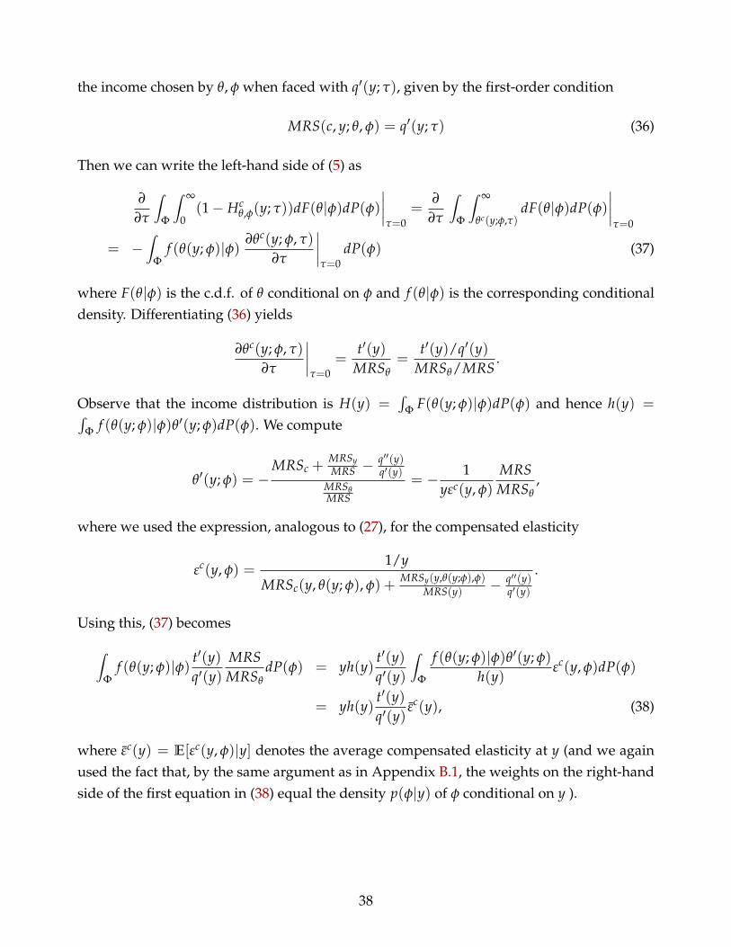
the income chosen by θ, φ when faced with q′(y; τ), given by the first-order condition

MRS(c, y; θ, φ) = q′(y; τ) (36)

Then we can write the left-hand side of (5) as

∂

∂τ

∫Φ

∫ ∞

0(1− Hc

θ,φ(y; τ))dF(θ|φ)dP(φ)∣∣∣∣τ=0

=∂

∂τ

∫Φ

∫ ∞

θc(y;φ,τ)dF(θ|φ)dP(φ)

∣∣∣∣τ=0

= −∫

Φf (θ(y; φ)|φ) ∂θc(y; φ, τ)

∂τ

∣∣∣∣τ=0

dP(φ) (37)

where F(θ|φ) is the c.d.f. of θ conditional on φ and f (θ|φ) is the corresponding conditionaldensity. Differentiating (36) yields

∂θc(y; φ, τ)

∂τ

∣∣∣∣τ=0

=t′(y)

MRSθ=

t′(y)/q′(y)MRSθ/MRS

.

Observe that the income distribution is H(y) =∫

Φ F(θ(y; φ)|φ)dP(φ) and hence h(y) =∫Φ f (θ(y; φ)|φ)θ′(y; φ)dP(φ). We compute

θ′(y; φ) = −MRSc +

MRSyMRS −

q′′(y)q′(y)

MRSθMRS

= − 1yεc(y, φ)

MRSMRSθ

,

where we used the expression, analogous to (27), for the compensated elasticity

εc(y, φ) =1/y

MRSc(y, θ(y; φ), φ) +MRSy(y,θ(y;φ),φ)

MRS(y) − q′′(y)q′(y)

.

Using this, (37) becomes

∫Φ

f (θ(y; φ)|φ) t′(y)q′(y)

MRSMRSθ

dP(φ) = yh(y)t′(y)q′(y)

∫Φ

f (θ(y; φ)|φ)θ′(y; φ)

h(y)εc(y, φ)dP(φ)

= yh(y)t′(y)q′(y)

εc(y), (38)

where εc(y) = E[εc(y, φ)|y] denotes the average compensated elasticity at y (and we againused the fact that, by the same argument as in Appendix B.1, the weights on the right-handside of the first equation in (38) equal the density p(φ|y) of φ conditional on y ).

38

As for the right-hand side of (5), we have

∫Φ

∫ ∞

0(1− Hθ,φ(y))

(βθ,φ − 1− ∂

∂I

∫ ∞

0t′(z)

(1− Hθ,φ(z; I)

)dz)

dF(θ|φ)dP(φ)

=∫

Φ

∫ ∞

θ(y;φ)

(βθ,φ − 1− ∂

∂I

∫ y(θ;φ,I)

0t′(z)dz

)dF(θ|φ)dP(φ)

=∫

Φ

∫ ∞

θ(y;φ)

(βθ,φ − 1− ∂y(θ; φ, I)

∂It′(y(θ; φ))

)dF(θ|φ)dP(φ).

Again using ∂y(θ(y; φ); φ, I)/∂I = −η(y, φ)/q′(y), this becomes after changing variables inthe inner integral

∫Φ

∫ ∞

y

(βθ(z;φ),φ − 1 + η(z, φ)

t′(z)q′(z)

)f (θ(z; φ)|φ)θ′(z; φ)dzdP(φ)

= −∫ ∞

y

∫Φ

(1− βθ(z;φ),φ

)dP(φ|z)dH(z) +

∫ ∞

y

∫Φ

η(z, φ)dP(φ|z) t′(z)q′(z)

dH(z)

= −∫ ∞

y

(1− βz

)dH(z) +

∫ ∞

yη(z)

t′(z)q′(z)

dH(z) (39)

where η(y) is the average income effect and βy the average social welfare weight at y. Equat-ing (38) and (39) and following the same steps as in Appendix A delivers the results.

B.4 Extensive-Margin Choices

Denoting by y(θ) the preferred labor supply of an individual of type θ among all y > 0, thisindividual will choose y(θ) instead of y = 0 if and only if

ϕ ≤ ϕθ(q)

where ϕθ(q) is such that

U(q(y(θ)), y(θ); θ) = u(q(0); θ, ϕθ(q)).

Let the distribution of ϕ conditional on θ be given by Γ(ϕ|θ) and denote the correspondingconditional density by γ(ϕ|θ). Then a share Γ(ϕθ(q)|θ) of all θ-types will supply y(θ) andthe rest y = 0. Hence, we can write the left-hand side of (5) as

∂

∂τ(1− Hc(y; τ))

∣∣∣∣τ=0

=∂

∂τ

∫ ∞

θc(y;τ)Γ(ϕc

θ(q; τ)|θ)dF(θ)∣∣∣∣τ=0

= −Γ(ϕθ(y)(q)|θ(y)) f (θ(y))∂θc(y; τ)

∂τ

∣∣∣∣τ=0

+∫ ∞

θ(y)γ(ϕθ(q)|θ)

∂ϕcθ(q; τ)

∂τ

∣∣∣∣τ=0

dF(θ) (40)

39

Note that the density of y is now h(y) = Γ(ϕθ(y)(q)|θ(y)) f (θ(y))θ′(y), so the first term is thestandard one derived in Appendix A. Integrating the variation defined in (10), we have

q(y; τ) = q(y)− q(0) + τ(t(y)− t(0)),

so we can write∂ϕc

θ(q; τ)

∂τ

∣∣∣∣τ=0

= (t(y(θ))− t(0))∂ϕc

θ(q)∂(q(y)− q(0))

.

Using this, the second term in (40) becomes

∫ ∞

θ(y)(t(y(θ))− t(0))γ(ϕθ(q)|θ)

∂ϕcθ(q)

∂(q(y(θ))− q(0))dF(θ) =

∫ ∞

y

t(z)− t(0)q(z)− q(0)

ρc(z)dH(z) (41)

where ρc(y) is the compensated participation elasticity at y.The right-hand side of (5) becomes

∫ ∞

θ(y)

∫ ϕθ(q)

−∞(βθ,ϕ − 1)dΓ(ϕ|θ)dF(θ)− ∂

∂I

∫ ∞

θ(y)

∫ y(θ;I)

0t′(z)dzΓ(ϕθ(q; I)|θ)dF(θ). (42)

The first term can be rewritten as∫ ∞

θ(y)(βθ − 1)Γ(ϕθ(q)|θ)dF(θ) with

βθ =∫ ϕθ(q)

−∞βθ,ϕ

dΓ(ϕ|θ)Γ(ϕθ(q)|θ)

= E[βθ,ϕ|θ, ϕ ≤ ϕθ(q)

]and hence, after changing variables, as∫ ∞

y(βz − 1)dH(z)

(where we slightly abused notation to write βy = βθ(y)).The second term in (42) equals

−∫ ∞

θ(y)

∂y(θ; I)∂I

t′(y(θ))Γ(ϕθ(q)|θ)dF(θ)−∫ ∞

θ(y)(t(y(θ))− t(0))γ(ϕθ(q)|θ)

∂ϕθ(q; I)∂I

dF(θ).

(43)The first term here is again standard and the same as in Section 5. The second term in (43)can be combined with (41) to deliver the uncompensated extensive-margin response, i.e.

−∫ ∞

y

t(z)− t(0)q(z)− q(0)

ρ(z)dH(z).

40

Collecting all these results and equating the left- and right-hand side yields

−yh(y)t′(y)q′(y)

εc(y) =∫ ∞

y(1− βz)dH(z)−

∫ ∞

y

t′(z)q′(z)

η(z)dH(z) +∫ ∞

y

t(z)− t(0)q(z)− q(0)

ρ(z)dH(z)

and hence the condition in the main text.

41