\

I

I ■

Si MISCELLANEOUS PAPER S-71-9

CALCULATION OF STRESS AND STRAIN FROM TRIAXIAL TEST DATA ON UNDRAINED

SOIL SPECIMENS by

J. Q. Ehrgott

May 1971

Sponsored by Defense Atomic Support Agency

Conducted by U. S. Army Engineer Waterways Experiment Station, Vicksburg, Mississippi

ATIONALTECHNICAL APPROVED FOR PUBUC RELEASE; DISTRIBUTION UNLIMITED ^FORMATION SERVICE

«„„nqt.old. Va "151

•mjmvmmmx . <i.i..,„,_• **-«*** ^!.v ■- -V* *K f- ■'■

Unclassified Socnritr CU««ific«tioo

DOCUMENT CONTROL DATA -R&D (StcuHtr cUmtlllCMtm «/ llll». Zsdr ol mbmltmet mat InOmtlni mmatmtlim M farad »AMI A* otwrafj il««0

I. ORIGINATING ACTIVITY fCofporaM mitoae)

U. S. Amy Engineer Waterways Experiment Station Vicksburg, Miss.

U, RtPOHT UCURirv CLASSIFICATION

Unclassified I». CROUP

•■ REPORT TITLE

CALCULAUCH OF STRESS AMD STRAIN FROM TRIAXIAL TEST DATA ON UNDRAINED SOIL SPECIMENS

i. MIC«IPTIVI MOTum (Trv ot report mud MclMll» d*M*>

Final report •■ AUTHomiifTCn« aw». aMtw in/(/«i, kiiiwg

John Q. Ehrgott

• - ««..»OUT DATE

May 1971 7«. TOTAL NO. OF PAGES

63 7b. MO- OF REFf

ft. PROJECT HO.

•a. ORIGINATOR*« REPORT NIHTICRIS)

Miscellaneous Paper S-71-9

•ft. OTHER REPORT NOI» (Auf MB —port)

othmr wi—ftirR star mm* ft» mmmignmd

10. DISTRIBUTION STATEMENT

Approved for public release; distribution unlimited.

ii. SUPPLEMENTARY HOTEs paper presented at Eric C. Wan^ Symposium on Protective Structures Technology, Air Force Weapons Laboratory, Kirtlafrd AFB, N. Mex., 21-23 July 1970.

12. SPONSORING MILITARY ACTIVITY

Defense Atomic Support Agency Washington, D. C.

The formulation of constitutive relations for use in computerized analyses of free-field ground shock phenomena is based primarily on laboratory-determined material properties. These properties, as described by stress-strain relations, are not directly determined in the laboratory, but are derived through interpretation of load and deformation data measured by the experimenter. Throughout this paper, one laboratory test, the triaxial shear test, is used to illustrate the extent of inter- pretation required on raw data and the influence of this interpretation on recommended constitutive properties. Various techn. ques that have been developed to obtain stress-strain data from the triaxial test are reviewed along with current advances in measurement systems. Typical raw data are presented and calculations of axial, lateral, and volumetric strains are made based on a variety of empirical and theoret- ical approaches.('The results demonstrate that research and development efforts are still required in the area of material proper by testing in order to establish adequate confidence in the formulation of constitutive relations for ground shock calculations.

DD .T..1473 ■ ■••LACES DO FORM UTS. I JAN M. «MICH IS OMOL1TI re« ARMY USE. 85 Unclassified

■ftcufity Classification

Unclassified Security Classification

Ground shock

Shear tests

Soil stress-strain relations

Stress-strain measurement

Triaxial tests

86 Unclassified Security Classification

■**i..,.i« n* .< :^—-qpjpjfpj v w

MUHMMMIMM

MISCELLANEOUS PAPER S-71-9

CALCULATfON OF STRESS AND STRAIN FROM TRIAX1AL TEST DATA ON UNDRAINED

SOIL SPECIMENS by

J. Q. Ehrgott

May 1971

Sponsored by Defense Atomic Support Agency

Conducted by U. S. Army Engineer Waterways Experiment Station, Vicksburg, Mississippi

«RMY-MRC VICKSBURG. MISS.

APPROVED FOR PUBLIC RELEASE; DISTRIBUTION UNLIMITED

PlgrtgCH»!

ABSTRACT

The formulation of constitutive relations for use in computer-

ized analyses of free-field ground shock phenomena is based primarily

on laboratory-determined material properties. These properties, as

described by stress-strain relations, are not directly determined in

the laboratory, but are derived through interpretation of load and

deformation data measured by the experimenter. Throughout this paper,

one laboratory test, the triaxial shear test, is used to illustrate

the extent of interpretation required on raw data and the influence

of this interpretation on recommended constitutive properties. Vari-

ous techniques that have been developed to obtain stress-strain data

from the triaxial test are reviewed along with current advances in

measurement systems.

Typical raw data are presented and calculations of axial, lat-

eral, and volumetric strains are made based on a variety of empirical

and theoretical approaches. The results demonstrate that- research

and development efforts are still required in the area of material

property testing in order to establish adequate confidence in the

formulation of constitutive relations for ground shock calculations.

ftmmwiWfiH««*»'**" *«*»!*SÄ«ÄÄ(ijj$ä|8

g-^WW^w WP*l*>r?}>i*&Li Wf-gW,y^.JPfBHP«ffWI^tl^J^tli^WVBfSFVWm? WW'HI' yn^yjmjwwji

PREFACE

This paper was prepared for presentation at the Eric H. Wang

Symposium on Protective Structure Technology held at the Air Force

Weapons Laboratory, Kirtland Air Force Base, New Mexico, 21-23 July

1970. The subject matter presented herein was primarily intended

for those persons involved in the field of ground motion prediction,

but not necessarily familiar with the area of material property

determination.

The laboratory equipment and techniques described in this re-

port were developed in support of research on propagation of ground

shock through soil and rock being conducted by personnel of the

Soils Division, (J. S. Army Engineer Waterways Experiment Station

(WES), for the Defense Atomic Support Agency (DASA).

This report was prepared and presented by Mr. J. Q. Ehrgott,

Impulse Loads Section, Soil Dynamics Branch, Soils Division, WES.

Helpful comments and guidance were provided by Mr. J. G. Jackson,

Jr., Chief, Impulse Loads Section. Mr. R. W. Cunny was Chief of

the Soil Dynamics Branch and Mr. James P. Sale was Chief of the

Soils Division. Directors of the WES were COL Levi A. Brown, CE,

and COL Ernest D. Peixotto, CE. Technical Director was Mr. F. R.

Brown.

CONTENTS

ABSTRACT 3

PREFACE h

NOTATION -- 8

CONVERSION FACTORS, BRITISH TO METRIC UNITS OF MEASUREMENT 10

CHAPTER 1 INTRODUCTION - 11

CHAPTER 2 THE TRIAHAL TEST 13

2.1 Test Description 13 2.2 Measurement System 16 2.3 Measurement Errors 18 2.k Typical Results 20

CHAPTER 3 INTERPRETATION OF RAW DATA— 26

3.1 Determination of Volumetric Strain 26 3.1.1 Method V-l 28 3.1.2 Method V-2 - 29 3.1.3 Method V-3 30 3.1.U Method V-4- - 31 3.1.5 Method V-5 31 3.1.6 Method V-6 - 32 3.1.7 Summary 32

3.2 Determination of Deviator Stress and Strain 33 3.2.1 Method S-l - 35 3.2.2 Method S-2 - 36 3.2.3 Method S-3 36 3.2.U Method S-k 37 3.2.5 Method S-5 - 38 3.2.6 Method S-6 39 3.2.7 Summary ■ —- 39

CHAPTER k DISCUSSION OF INTERPRETATION METHODS 58

^.1 Comparison for Hydrostatic Tests 58 k.2 Comparison for Shear Tests 62

CHAPTER 5 CONCLUSION - 73

REFERENCES - 75

FIGURES

2.1 Data available from the triaxial test 22 2.2 Schematic of WES high-pressure triaxial test device 23

5

!

■»«tu <»>¥»cf» ftwflilh '■*' -

$ygfc$si»

2.3 Typical constant p-type triaxLal test results for a sandy clay 24

2.4 Typical constant a -type triaxial test results for a siltstone 25

3.1 Deformed shapes of specimens during hydrostatic loading 4l 3.2 Triaxial specimen of recompacted clayey silt after being

subjected to 500-psi hydrostatic pressure, shape IC 42 3.3 Triaxial specimen of recompacted clayey silt after being

subjected to 5»000-psi hydrostatic pressure, shape IC 43 3.4 Triaxial specimen of a silty clay with rock fragments after

being subjected to 1,000-psi hydrostatic pressure, shape IIA > 44

3.5 Triaxial specimen of silty clay with rock fragments after being subjected to 5,000-psi hydrostatic pressure, shape IIA 45

3.6 Cross section of shapes considered in Method V-l— 46 3-7 Cross section of assumed shape used in Method V-2 46 3-8 Cross section of assumed shape used in Method V-3 46 3-9 Assumed shape used in Method V-4 46 3.10 Summary of methods used to calculate volumetric strain i"f 3.11 Shapes of failed specimens after shear test 48 3.12 Triaxial specimen of sandstone after shear failure during

a dynamic constant p-type test, shape IIA 49 3.13 Triaxial specimen of recompacted clayey silt after being

subjected to a small deviator stress while maintaining a confining pressure of 5>000 psi 50

3.14 Triaxial specimen of modeling clay prior to test 51 3.15 Triaxial specimen of modeling clay after application of a

small deviator stress while a confining pressure of 5»000 psi is maintained 52

3.16 Triaxial specimen of modeling clay after application of a larger deviator stress while a confining pressure of 5,000 psi is maintained 53

3.17 Triaxial specimen of modeling clay after application of large (postyield) deviator stress while a confining pres- sure of 5,000 psi is maintained ■ 54

3.18 Specimen deformation during shear test 55 3.19 Cross section of specimen showing assumed deformed shapes

considered in Method S-l ■ 56 3.20 Cross section of assumed deformed shape considered in

Method S-2 - - 56 3.21 Cross section of assumed deformed shape considered in

Method S-4 - - 56 3.22 Distribution of axial strain along length of a specimen 56

WUß^f^^W^ [.■• »" ""I •-I" W

I ^S«aB*?J^^'>'^^rv .^■iV^*-'****^

4.3

4.4 4.5

4.6 4.7

Summary of methods used to calculate deviator stress and strain 57 Comparison of methods used to calculate volumetric strain for the sandy clay test 66 Comparison of methods used to calculate volumetric strain for the siltstone test 67 Comparison of methods used to calculate deviator stress and deviator strain for the sandy clay test 68 Initial portion of plots shown in Figure 4.3 69 Comparison of methods used to calculate deviator stress and deviator strain for the siltstone test 70 Initial portion of plots shown in Figure 4.5 71 Comparison of methods used to calculate volumetric strain during shear for the siltstone test 72

■<

;£j vi&mJ3***&amSi **^l)^i^^*»^^'™^™*{-**<-*^^™K~-s~^^<...^*~**:^t .. '',,. i£;

NOTATION

A Area; also, calibration error

A Original area; also, fixed area of ends of test specimen

A, Current area at midheight of test specimen

B Output error

C Overall accuracy of measurement device

D Diameter of test specimen

D Original diameter of test specimen

D. Current diameter of test specimen at midheight during

hydrostatic test

D2 Current diameter of test specimen at midheight during

shear test

E Young's modulus

G Shear modulus

H Height of test specimen

H Original height of test specimen

H, Current height of test specimen during hydrostatic test

Hp Current height of test specimen during shear test

K Bulk modulus

p Mean normal stress

R Operator error

V Volume of test specimen

V Current volume of test specimen during hydrostatic test

8

>:#

%

AV/V O

AV

€ - € a r

a - a a r

Original volume of test specimen

Corrected original volume of test specimen

Deformed volume of test specimen at end of hydrostatic test

Deformed volume of test specimen during shear test

Volumetric strain

Volume change

Axial strain

Radial strain

Tangential strain

Deviator strain

Axial stress

Radial stress; also, confining pressure

Tangential stress

Deviator stress

»mmmmme&itgQigijjtffcgt'

CONVERSION FACTORS, BRITISH TO METRIC UNITS OF MEASUREMENT

British units of measurement used in this report can be converted to metric units as follows.

Multiply By To Obtain

mils 0.0254 millimeters

inches 2.5U centimeters

-feet 0.301*8 meters

pounds per square inch O.070307 kilograms per square centimeter

pounds per cubic foot 16.01846 kilograms per cubic meter

10

CHAPTER 1

IHTRODÜCTION

The response of any land-based structure to loadings produced by

the explosive impact resulting from either conventional high explosive

(HE) or nuclear detonations is highly dependent upon the dynamic

stress-strain and strength characteristics of the surrounding and

supporting earth material. Current wave-propagation computer codes

used in the prediction of free-field stresses and motions require

stress-strain constitutive relations for the earth materials at the

sites of interest. Generally, such relations are derived from labo-

ratory tests on undrained soil and/or rock specimens conducted under

a variety of states of impulsive-type stress and at magnitudes closely

simulating expected field levels. In cases where current equipment

limitations only allow the application of static loadings, extrapola-

tion of test results must be made to reflect dynamic conditions.

The derivation of stress-strain properties from laboratory data,

however, is subject to analysis and interpretation by the experi-

menter. It is the intent of this paper to illustrate, by examples,

the influence that analyses and interpretations have on stress-strain

relations obtained from raw test data. It is realized that a con-

tinuing effort is being made to solve and/or improve the uncertainties

affecting laboratory tests; however, the techniques presented herein

are representative of the approaches currently being used to obtain

stress-strain relations during production-type testing programs.

In order to best illustrate how the raw data are analyzed, one

laboratory test, the triaxial shear test, will be used throughout

this paper; similar illustrations can be obtained from any other lab-

oratory test based on its peculiar limitations and problems. Since

many of those involved with the development of constitutive relations

11

mmmmmmiiMiHiffl&fä^

may be unfamiliar with some areas of laboratory techniques, Chapter 2

of this paper will present a general review of the triaxial test and

recent advances made in measurement systems. In Chapter 3» various

methods used to calculate volumetric strain, deviator stress, and

deviator strain from raw data will be derived, and in Chapter k,

stress-strain relations derived using the various calculation methods

and raw data obtained from two triaxial tests will be compared and

discussed.

12

s*.Mi'-' iJ*,^-1 '■."

I

CHAPTER 2

THE TRIAXIAL TEST

■■:■■:

■il

I* J A

2.1 TEST DESCRIPTION

The triaxial test, when properly instrumented so as to provide

complete load and defo aation data, is oie method for determining

soil and rock stress-strain behavior and shear strength. Because

triaxial test equipment is designed to permit separate control of

both lateral and axial loadings, the test can provide data on the

fundamental response characteristics of soil and rock under a wide

variety of controlled states of stress. In addition to stress con-

trol, the test also permits control of loading rate, drainage condi-

tions, and specimen size. A brief history of the development of the

triaxial test is contained in ASTM Special Technical Publication

Number 361 (Reference l), and a detailed description of the apparatus

and test procedure is contained in Reference 2.

Separate pressure control systems are necessary for application

of the several possible axial and lateral stress paths. Application

of the axial lead can be accomplished by any number of methods de-

pending on whether the test is desired to be stress-controlled or

strain-controlled. When the specimen is to be loaded to failure, a

strain-control method should be employed; when the behavior of the

specimen is to be studied at less-than-failure stress levels, a

stress-control method is preferable because of theXregulation required

in loading increment. Dead loading the sample, eitheKdirectly or by

lever systems, is probably the oldest and simplest stressXcontrol

method. Pneumatic systems that apply air pressure to a movable piston

can be used to develop not only very large loads (by varying the pis-

ton area ratio) but also to develop rapid loading rates. Hydraulic

systems employ the same principle but are best suited for strain-

control testing. The use of motor-driven gears is also a very

13

i I

effective method of applying a strain-controlled load. Vibratory-

loads can be achieved by means of a rotating cam system, a pneumatic

system employing a sequence valve, springs with a deadweight loading

device, and electrically controlled devices. Shock loadings can be

accomplished by dropping weights, pneumatic loading systems, or ex-

plosive charges.

Confining pressures can be achieved by means of any number of

systems employing air compressors, hydraulic pumps, bottled gas, or

piston-type multipliers. At lower pressure levels (less than 500

psi ), the use of gas as a chamber fluid provides easy control of

the confining pressure. At higher pressures, a hydraulic fluid must

be used for reasons of safety; however, a hydraulic fluid becomes

difficult to control as the specimen changes in volume and a more

complex supply system is required.

In the standard triaxial configuration, the specimen is placed

in a cylindrical chamber. The axial load is applied to the specimen

by a piston, which enters through a sealing device (piston guide) in

the top of the triaxial cell. The inside of the chamber can be pres-

surized to provide a lateral loading or confining pressure on the

specimen. Generally, the cylindrical specimen is sealed from the

chamber fluid by a thin membrane, and the specimen is sandwiched be-

tween two rigid plates that provide the transfer of load between the

piston and the specimen.

The triaxial specimen has a cylindrical shape with a height-to-

diameter ratio of approximately 2:1. Axial load is applied in the

vertical direction or along the z axis. Lateral loading is applied

radially around the specimen or along the r axis. In the general

analysis of the triaxial specimen, it is assumed that the tangential

stress and strain are equal in magnitude to the radial stress and

A table of factors for converting British units of measurement to

metric units is presented on page 10.

Ik

I strain (i.e., <ra = or , e„ = e ) and that the stress and strain dis-

o r o r tribution throughout the specimen is uniform. Although investiga-

tions such as those in References 3 and k have shown that stress and

strain distribution within triaxial specimens is generally not uni-

form, the uniformity assumptions are currently necessary to the over-

all analysis of the test results.

Since the specimen is completely within the chamber during load-

ing, the confining pressure a not only acts radially on the speci-

men, but also vertically. Hence, the axial loading on the specimen

is the sum of the axial force of the piston p and the axial force

exerted by the confining pressure. The total axial force divided by

the specimen area (perpendicular to direction of loading) is defined

as the axial stress a a Soil mechanists define the difference be-

tween the axial si ess and the confining pressure as the deviator

stress (o - a ). v a r' Assuming for the moment that the test specimen is elastic, homo-

geneous, and isotropic and deforms as a cylinder. Figure 2.1 illus-

trates some of the states of stress that can be imposed on the speci-

men along with typical stress-strain responses. For a hydrostatic

state of stress where 0=0 . the mean normal stress p = a r '

a +20 a r

increases and the deviator stress (o" - o ) remains zero. The spec- v a r' imen response is usually plotted as a pressure-volumetric strain

curve, whose slope is the bulk modulus k . In a shear test, the

specimen is first loaded hydrostatically to some level of p . In

cases where the confining pressure is held constant while the devia-

tor stress is increased, the specimen response is usually plotted as

a deviator stress versus axial strain e curve, the slope of which

is Young's modulus E . In cases where the confining pressure is

decreased while the axial stress is increased so that the mean normal

15

yr-nfiitifrSiyrilrrr rMff^ffifffMCtflW^* W>iN-»'ffr^

stress is held constant, the response is usually plotted as a de-

viator stress versus deviator strain (e - e ) curve, the slope of

which is two times the shear modulus G . In addition to the modu-

lus data, yield strength can also be obtained. Several shear tests

conducted at different levels of p provide data to describe a yield

envelope.

Of course, many other variations can be conducted, such as the

extension test in which the confining pressure is held constant and

the axial stress is decreased. Yield strength values obtained from

such tests describe a lower bound yield envelope.

2.2 MEASUREMENT SYSTEM

At the heart of any test device is the measurement system that re-

ports the specimen's response. In the triaxial test, as in most tests

designed to obtain earth material properties, there is no one universal

measurement system because of the broaa range of loads and deformations

encountered. The system that will be presented is unique to the U. S.

Army Engineer Waterways Experiment Station (WES) and used mainly for

soils and soft rocks; several individual units are used for various

measurement ranges.

The static confining pressure felt by the specimen can be meas-

ured by a number of commercially produced items such as pressure

transducers and gages. In a dynamic test, special pressure trans-

ducers are mounted within the confining chamber«

The axial load is best measured directly on the soil specimen to

eliminate the influence of piston friction, especially during high-

pressure cyclic tests. The internal load cell must be precalibrated

for pressure effects, however. In a dynamic test, two load cells are

used (one above and one beneath the specimen) to provide a cross ref-

erence as well as to monitor wave propagation in those tests in which

16

imw+ujUiW"* ;■:»-..U..JUUU.,. .-" -m--^.-.

the specimen might be loaded too fast.

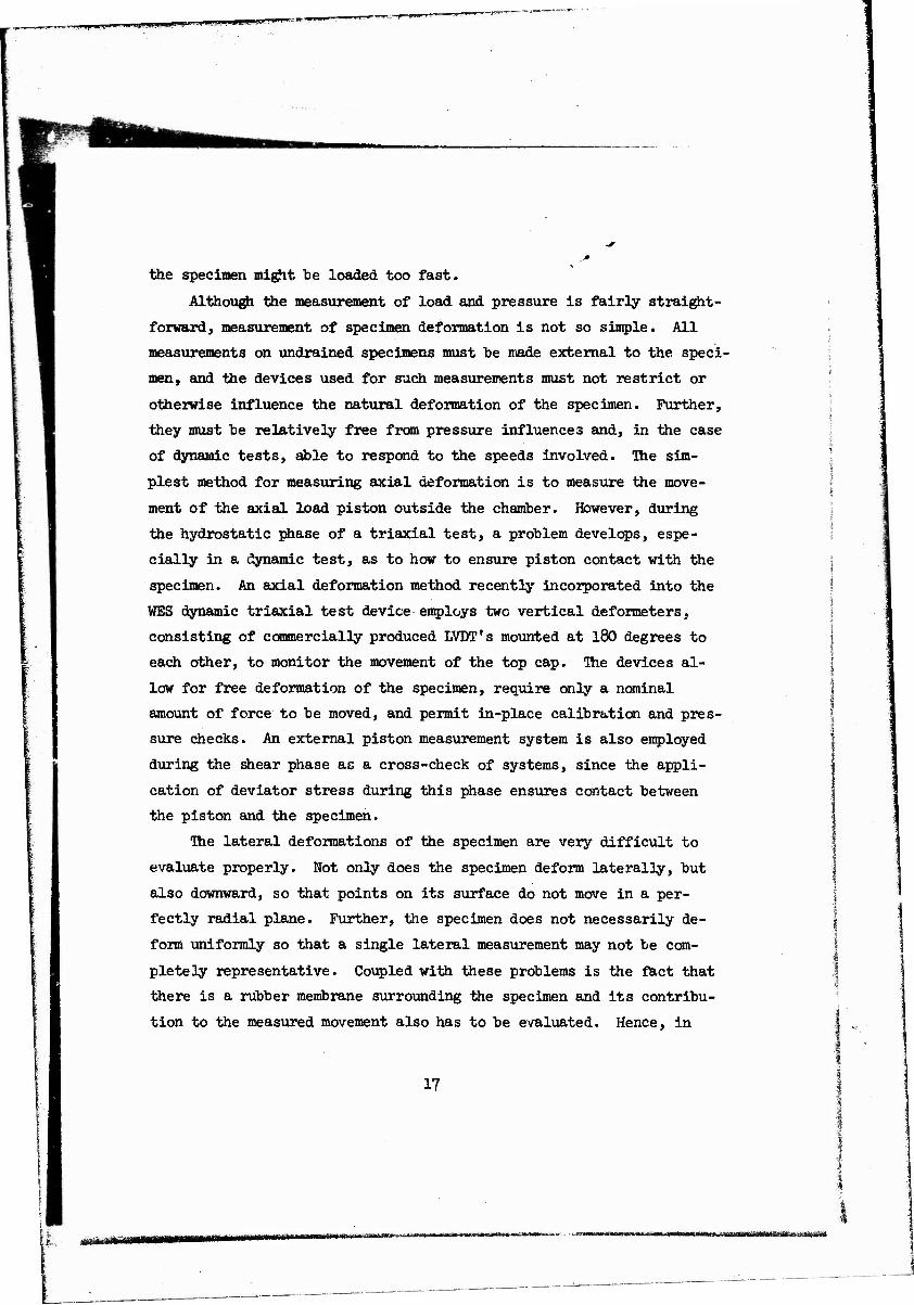
Although the measurement of load and pressure is fairly straight-

forward, measurement of specimen deformation is not so simple. All

measurements on undrained specimens must be made external to the speci-

men, and the devices used for such measurements must not restrict or

otherwise influence the natural deformation of the specimen. Further,

they must be relatively free from pressure influences and, in the case

of dynamic tests, able to respond to the speeds involved. The sim-

plest method for measuring axial deformation is to measure the move-

ment of the axial load piston outside the chamber. However, during

the hydrostatic phase of a triaxial test, a problem develops, espe-

cially in a dynamic test, as to how to ensure piston contact with the

specimen. An axial deformation method recently incorporated into the

WES dynamic triaxial test device employs two vertical deformeters,

consisting of commercially produced LVDT's mounted at l80 degrees to

each other, to monitor the movement of the top cap. The devices al-

low for free deformation of the specimen, require only a nominal

amount of force to be moved, and permit in-place calibration and pres-

sure checks. An external piston measurement system is also employed

during the shear phase as a cross-check of systems, since the appli-

cation of deviator stress during this phase ensures contact between

the piston and the specimen.

The lateral deformations of the specimen are very difficult to

evaluate properly. Not only does the specimen deform laterally, but

also downward, so that points on its surface do not move in a per-

fectly radial plane. Further, the specimen does not necessarily de-

form uniformly so that a single lateral measurement may not be com-

pletely representative. Coupled with these problems is the fact that

there is a rubber membrane surrounding the specimen and its contribu-

tion to the measured movement also has to be evaluated. Hence, in

17

w^mmmbmmmmmmm^mits0muusiiif^tSä^imi6S^

u

order to make any measurement of strain in the radial direction, some

problems have to he neglected during the actual test measurements and

then accounted for during evaluation of results.

Of the many devices •which have been developed for measurement of

lateral strain, the one described in Reference 5 appears to be the

best suited for static tests. The device measures changes in diameter

of the specimens by means of cantilever springs, which are instru-

mented with electrical resistance strain gages. The lateral defor-

meter is simple in design, easy to install, and exerts little if any

force on the specimen. Several of these devices can be arranged at

different elevation levels around the specimen so that a fairly com-

plete deformation profile can be obtained. Also, and most important,

the device allows for in-place calibration, including that for pres-

sure effects. Another system, utilizing commercially produced LVDT's,

is best employed for tests in which the confining pressure is dynami-

cally applied. This device has physical limitations, such as range,

and it is easily damaged during uncontrolled specimen rupture.

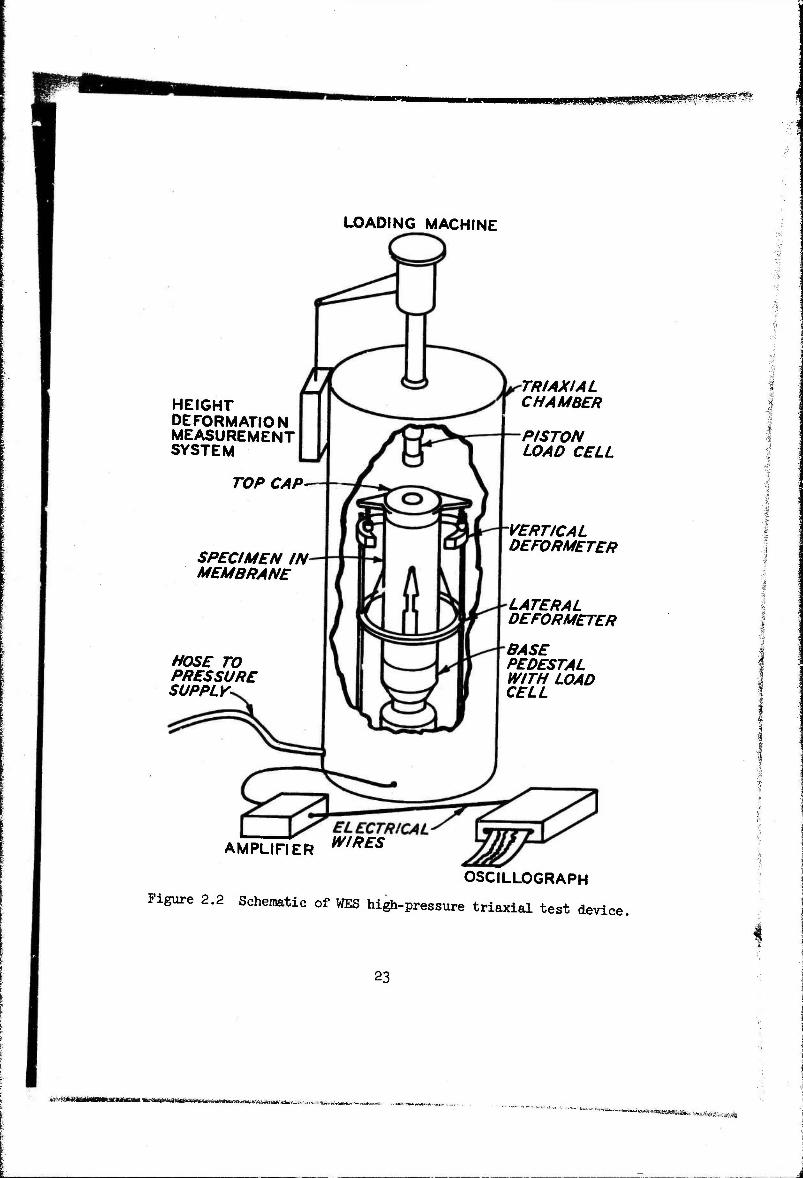
Figure 2.2 shows a cutaway schematic of the WES high-pressure

triaxial test chamber with the measurement system in place around the

specimen. The electrical outputs from the various systems go through

amplifiers and are recorded on a direct-writing, light-beam

oscillograph.

2.3 MEASUREMENT ERRORS

For a given measurement device, there are generally three sources

of error, i.e. calibration error, output error, and operator error.

Calibration error (+A) is related to the accuracy of the device used

as a standard and the associated errors that occur during the calibra-

tion; +2 percent is reasonable in a production-type program. Output

error (+B) is a function of the measuring device and system including

18

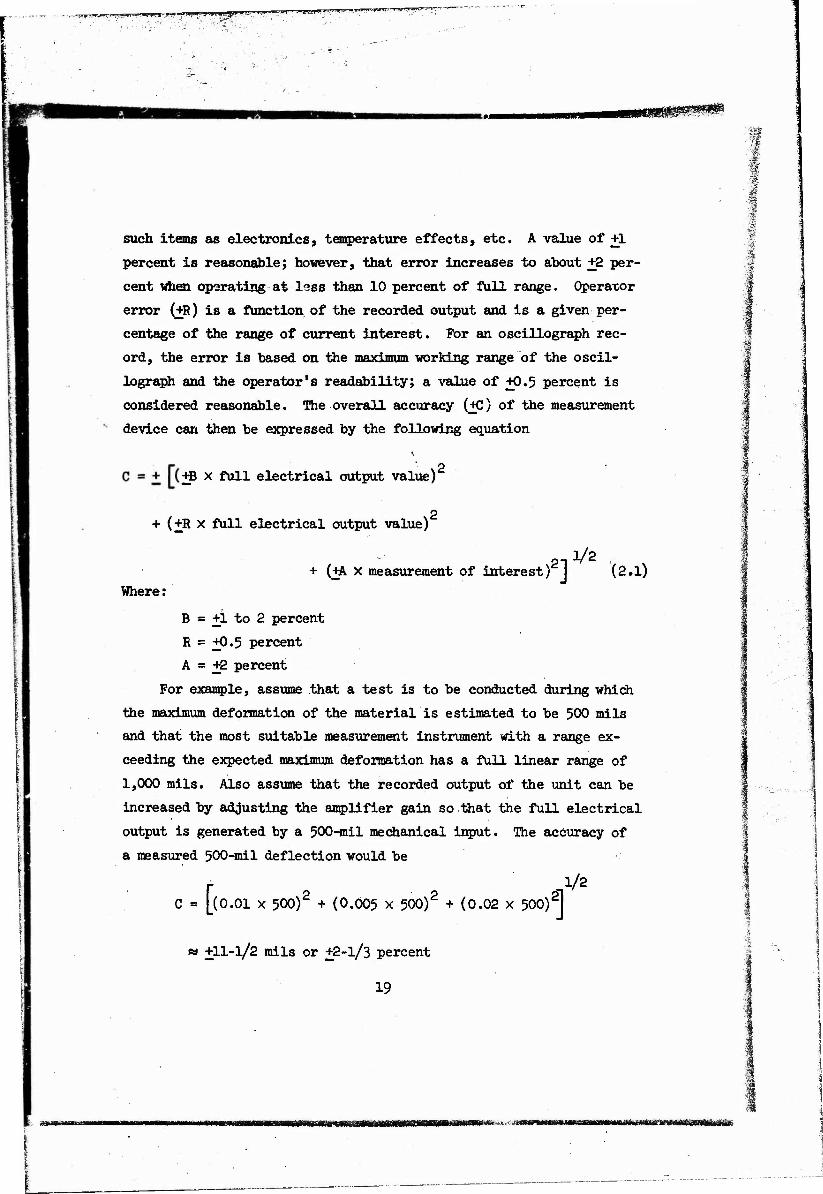
such items as electronics, temperature effects, etc. A value of +1

percent is reasonable; however, that error increases to about +2 per-

cent when operating at less than 10 percent of full range. Operator

error (+R) is a function of the recorded output and is a given per-

centage of the range of current interest. For an oscillograph rec-

ord, the error is based on the maximum working range of the oscil-

lograph and the operator's readability; a value of +0.5 percent is

considered reasonable. The overall accuracy (+C) of the measurement

device can then be expressed by the following equation

•• 2

+B x full electrical output value)

+ (+R x full electrical output value)'

1/2 + (+A X measurement of interest) 1 (2.1)

Where:

B = +i to 2 percent

E = +0.5 percent

A = +2 percent

For example, assume that a test is to be conducted during which

the maximum deformation of the material is estimated to be 500 mils

and that the most suitable measurement instrument with a range ex-

ceeding the expected maximum deformation has a full linear range of

1,000 mils. Also assume that the recorded output of the unit can be

increased by adjusting the amplifier gain so that the full electrical

output is generated by a 500-mil mechanical input. The accuracy of

a measured 500-mil deflection would be

1/2 - [(0.01 x 500)2 + (0.005 x 500)2 + (0.02 x

» +11-1/2 mils or +2-l/3 percent

19

500)2]

Ifj however, the actual maximum deformation of the specimen is only

50 mils or even if the specimen deformed 5OO mils, Taut data are re-

quired at the initial part of the test, say at the 50-mil deformation

point, then the accuracy of the measured 50-mil deformation would be

1/2 C = [(0.02 x 500)2 + (0.005 X 5OO)2 + (0.02 x 50)2]

« +10-1/3 mils or +21 percent

It can be noted from the above examples that care must be taken

to delect measurement instruments that provide the greatest possible

accuracy over the range of interest. The selection depends on two

factors: experience in estimating material response behavior and a

predetermined measurement objective such as to obtain initial stress-

strain data or to obtain data at the maximum or yield condition.

2,k TYPICAL RESULTS

The recorded load and deformation time histories are converted,

through a set of analytical assumptions, to stress and strain his-

tories and displayed for further property analyses in the form of

stress-strain plots. Two typical WES static high-pressure triaxial

test data plates are shown in Figures 2.3 and 2.*+; Figure 2.3 illus-

trates results for a constant p-type test conducted on a sandy clay

specimen and Figure 2.U illustrates results from a constant a -type

test conducted on a clayey siltstone. The sandy clay specimen (Fig-

ure 2.3) was first loaded hydrostatically to 1,000 psi and then

loaded to failure in shear by increasing the deviator stress while

the mean normal stress was maintained constant. The siltstone speci-

men (Figure 2.k) was hydrostatically loaded to 1,500 psi and then

loaded to failure in shear by increasing the deviator stress while

20

-äL<S^\i^l.i,V_ :.äMt.i>Ki=aü:

mmmmimmmmm®i@%®x

the confining pressure was held constant. The response of each speci-

men to the hydrostatic loading is seen as a plot of pressure versus

volumetric strain, and the response to the shear loading is seen as

a plot of deviator stress versus deviator strain. Pertinent informa-

tion regarding the composition properties of the specimens is also

shown on the figures.

21

MffaiW^'liri^JWn ill

**i»*Mmlm*ltmK, Säjs äii^*««*>»i«ias.i.aMte,,,>

_J

'■:*' ■' ■■■..*". .%

is (Lu

O Zl

Z o

ujtr CO LU O

^-Vf (Jfb-^H

(J* - Dx>)+

Id

£ b

<irr

< b-

i 11M MM

MtIM

<^o

{'* - °*) + (10 - "o)+

i- Q 5 «

a iy U)

? < < fc HI ui z a

b o b 5

e • u ..

b°2b'

+ fr-V

a Q ui 1- UI 55 Z "> < < <. ui p UI S ■n tt. o s <J m V. O 'o UI

b O b Q

cr <

X <n

< a: z ÜJ

b'

fek

♦ M MM

-P «n

-p

•3 1 )H -P

a> H ■3 H

I

H cvj

I P-4

TSHHM b"

22

i»«fUtf*U<WR, IHWyW'.«. US^Kr1<M)U0ä(äkUiU

fl^öRRM^IPM^^^

HEIGHT DEFORMATION MEASUREMENT SYSTEM

TOP CAP

SPECIMEN IN MEMBRANE

LOADING MACHINE

HOSE TO PRESSURE SUPPLY*

TR I AXIAL CHAMBER

PISTON LOAD CELL

VERTICAL DEFORMETER

LATERAL DEFORMETER

BASE PEDESTAL WITH LOAD CELL

EL ECTRICAL AMPLIFIER W,RES

OSCILLOGRAPH

Figure 2.2 Schematic of WES high-pressure triaxial test device.

*

23

MaMSMMHUWintiWl HWWWUlaHUaMMWMinsu tt*.sa«'«*üi.'ii.>w-'

■atom«**.. -.N»¥^«,..,j>t

IM *'o- °0 ttaMXf U01VIASQ

O O s n 8 s

< z I- «I c

> M a

•H "

5

a£

STE 3« K «9< * < ■ « O j o o ■

T

5 0.

ii

h z < (0 z o 0

5H o<

?8 er •

s vo oc

a H d Su

J < s (T DO f • or t> « o c- <T er oc IT

r- c <\ <\ ev H O H

g fe. z z K u K

ft >- »- »-

(M 1- X

5 5 O s >

1-

Z M t- Z

> < r a

H

Z u s

a

1- < ■c

1- < Z

s ü o

u u 3 u M H 1- H a 1, o < < M «t > M » * w

I a er

3 IT

S IT £ i- er IT « O o o

liiiL i!

, ■

:::::::::::::::::::: w g i w

^4 "1 T 1

1 s [ i_ ^ i _j V

~^ L i \

::"""::::::::;:::::":::s: -- - i

::::_":":"":-_:::":":::IB jar

5? H ü

03 to

5H

O

10

s 03 <D U

-P W <u -p

P 3 SH -P

CD

s -p I

P) «J -p ir\ ö H cd

-p K w Z C

O Z o u

o a. H r> o cö rH >

> O

4 ß 3 H K 1-

o U 0O

IA Z <M u a>

h

8 cu o 3

o CV1

O 00 8 8

ISd ' ß - X> 'SS3MXS M01VIA3Q isd '4 '»nssaud OIAVISOMQAH

24

»jpr«;*fj«*w«*p^ ■-

iSd ''o - "o ttaMx« uoxviAaa

"T *

:::::::::::::::::: s * ' :.\z.:.z::........ z $ .:1,::.::::::::::: s ? __] | « -

:r: "::::::: : 5 2 .il:..::.::::: £'* » .: ±.:.::.::::::: r- 3. ::±::.:::::::::: b * , ...\ :::::: • > .__].. .____._. JB O , :::.L._::::::;::: 0 s ::::i::::::::::_: ._-.i.- —._.. — -----r---- ......l...:....:.z.::..z. .... .i:::::::::::::::::: ....:. .1.........zz.:.:.: :: L: .:::.::::::::, ::.::.::$::::::.:::::::.: ::::::::. s:::::::::::::::<

* L

h 1 ., ) '

" s ^ v j 1 _J ^ k ■

5 rt 1 •! 1

r-J ►•

i o

h- GJ ■p *> 5 ci 3

3 t

• c~ l/N 8

H •rt 8 ■rt 8 «I H ON +> O +> u .* -M) § CO ■H ■H fi * • 'S +3 CO & > a ■P S

•aj « d- ■ M

1 ■rt +> a

> *

Ö F- WO

«NT H rrt i !

| f •rt -rl

• ft *-

0

2! H * CO H s s+» 0 r

S 5 xo *** 1 8 < = «. i-ir

u C i i. ?8S a c c 0 < u -1 < U+J

< ■ 5 0 J 0 0 a t« t 0

T I 1 ' Jg

r f_x_ * ■«

■" * - Ä C "* » * ■* *

* * * Q __ ' * ^ Ö :::::":::» :::::::::::!£ :;:.:-_::: 2 "IIT::::::

i 5 i

b" i Q

K w

_z .. „0 0 1

I::::::::::::;::;:;::::::g ::::::::::::::::::::::::: g>

5 CO VO .5 Cv)

r« S* (T 1^ H

Ü * CO Of CO :* CVI

J:« 4 • u4 «Pi

CM H 0 BN 3 wu

J 5 1 0> ON «*" cu

O >o

1 4 « • • • z 01 H 0 m 3 H

CO CV)

„ h z z » O »» ft

V 1- 1-

X 1 5 0 s >

1-

z u z

> z

a> z u z Ü

s ü

p < < m 9

s 0

0 0 e M

0

ö H 5 1- < U < u ■

M « > «• • » «

CVI \o

CO lf\ t^ CVI m rr 0 -* in

4 • 01 0 O

i m %■

1 _ i" _i r ■* ■■ «

::::::::::::::: g s ::::-

:::-::::::_,::_ ^ 0 - , _ W

«1 II 11 j

1 * ^ ^L ^ r*

'.IZlZ'.ZZZZZlSZZZZZZ'.ZlZZl ::::::::!::::!>"""": ::::::::::::::.!s" ::.:::::: ::_s: ::: : .......zz 5» :::::::::::::.:::::\::± "I"IIIII"!"""" .;_" ::::::::::::::::: :.s:: .:: :_ _:\. .Z.^lZ.ZZt :„ J 888880 m 01 ON vo ro

o CO

ltd •'• o- o 'tsauis MoiviAaa isd 'd 'annssand OIIVISOUQAH

25

s O

W

■H W

O

w -p H

to tt>

CO a> -p

1

-p

B -p ■ o

p to C o o

o •H

s

aj (Ü

■H

^,^\'liLri3am*M1f^W"lnliyr■^rvr^■^^•"^^ t^K«BNaBHMfe. ^^^aftg^a>a*«wfli^^ « a**,* ^^.'itvmm^mm^^^äs^sm^^^^M^^^^m^

^J

CHAPTER 3

INTERPRETATION OF RAW DATA

' Between collection of the raw test data and the production of

data plots such as those shown in Figures 2.3 and 2.U, much inter-

pretation and analysis must be done by the material property investi-

gator. This analysis of the raw data has considerable influence on

the constitutive properties finally selected to describe the mate-

rial's behavior. The stress-strain plots shown in the above-

mentioned figures were based on a certain set of assumptions; other

stress-strain plots could have been generated from the same set of

raw data using different, yet perhaps equally valid, assumptions.

In the following section, some of the various methods and assumptions

that can be used to analyze raw data will be described. Then the data

from the two previously presented triaxial tests, one on a relatively

soft sandy clay (Figure 2.3) and one on a relatively stiff clayey

siltstone (Figure 2.k), will be used to illustrate the variations in

moduli that can be obtained using the different methods of analysis.

3.1 DETERMINATION OF VOLUMETRIC STRAIN

Since deformation measurements are made only at a few specific

locations on the specimen surface, it is necessary to assume a com-

plete specimen deformation pattern in order to describe the overall

stress-strain response of the specimen to imposed loadings. First,

consider some of the general deformed shapes noted during application

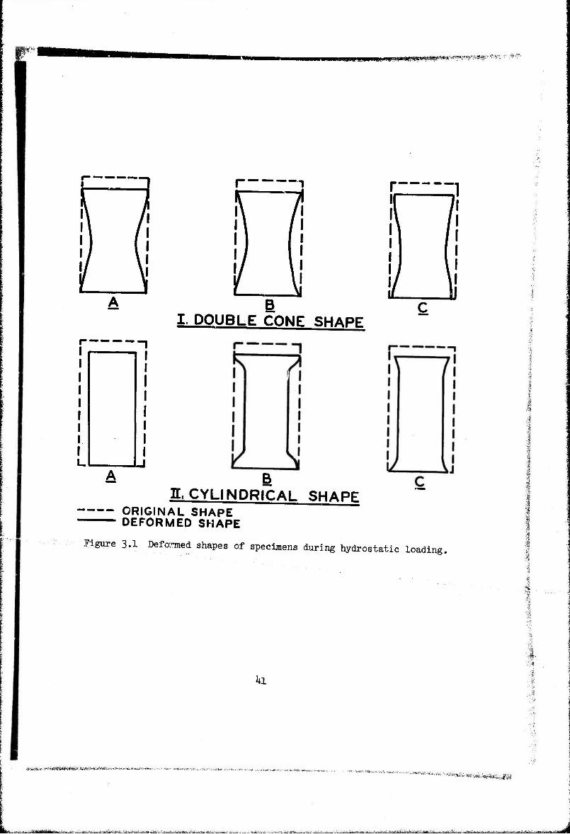
of hydrostatic loadings. Figure 3«1 shows the two most common shapes,

double cone and cylindrical. Specimens deforming as a double cone

(IA, IB, IC) undergo maximum lateral deformation at the center while

the ends undergo little or no lateral deformation. The deformation

restraint at the ends is attributed to end-cap friction (References

26

^^»«•WSSSSW5*: *c;S?"«SS??

6 and 7)• Shear forces at both ends caused by the top cap and base

pedestal prevent free movement of the specimen; however, the influ-

ence of end caps is not the same on all types of material. Figures

II-A, II-B, and II-C of Figure 3»1 show the second type or cylin-

drical shape. The specimens deform radially in a uniform or nearly

uniform manner. The effect of the end caps on the specimen is not as

apparent as in the case of the double-cone shape. There is little

factual data regarding the distribution of axial deformation through-

out the -specimens in either of the two cases, although it is surmised

that the distribution is more nearly uniform in the cylindrical shape.

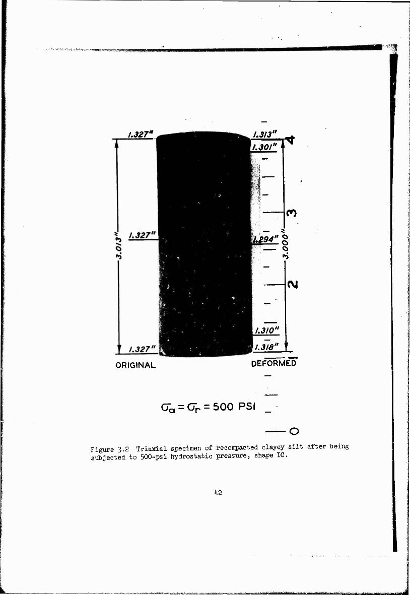
Figures 3«2 and 3«3 show two separate recompacted clayey silt

specimens after being subjected to confining pressures of 500 and

5,000 psi, respectively. Although some rebounding occurred, the

general deformed shape achieved after completion of loading remained

upon removal of the pressure. The shape is basically double cone

with some deformation of the ends as typified in Figure I-C of Fig-

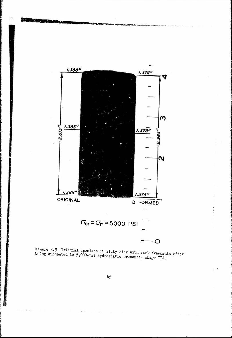
ure 3«1« Figures 3-^ and 3»5 show deformed specimens of silty clay

with rock fragments after hydrostatic loading to pressures of 1,000

and 5*000 psi, respectively. Note that these specimens deformed as

fairly uniform cylinders as typified in Figure II-A of Figure 3.1.

All of the above specimens were tested in the same manner; thus the

differences in deformed shape can only be attributed to the physical

properties of the specimen material. Each type material, therefore,

should be considered separately in analyses.

To illustrate the various approaches that can be used to calcu-

late volumetric strain, consider only one of the deformed shapes as

shown in Figure 3«1« In this case the specimen starts from an ini-

tial shape of a uniform right circular cylinder whose volume V o

is i

27

vo - ? (V2 <V ^ Where:

D = original diameter o H = original height

The specimen then deforms as a double cone with fixed ends, i.e.,

shape I-B. Throughout the example, compression will he considered as

positive and all strains will be calculated in Lagrangian notation,

i.e. (change in dimension)/(original dimension). Saw data measure-

ments include pressure p , total height change AH , and total diam-

eter change AD at midheight of the specimen.

3.1.1 Method V-l. In this method, the deformed shape is approx-

imated by straight lines and hence, two truncated cones placed end to

end as shown in Figure 3.6. The volume V of the specimen at any-

given time, i.e. the current volume is

Vc = Vo-AV = iHl(Ai+Ao + Wo") (3*2)

Where:

D- = current diameter at midheight = D - AD

V = initial volume = H A 0 00

H.. = current height = H - AH ^2 1 O TTD-

A.. = current area at midheight = -j-—

3he

p r A_ = fixed area of ends = -r—

AV The volumetric strain — can be found from o

V - V AV o c

o o

H.

4 o o 3 Vil VJk O 10/ /o o\ nD2t

0 O TjDH

28

:^.r?*iÄrt^^w;.*A*i,j, A

PSPB

Substitutions can, of course, be made to allow comparison of

volumetric strain in terms of axial and radial strains, i.e.

« = axial strain - ^ a H o

€r = radial strain = ^ o

H. = H - e H J. o a o

i o r o

(3.U)

(3-5)

(3.6)

(3.7)

and the volumetric strain for Method V-l becomes

Al. D;TI - (H - e H ) i |(D - e D )2 + D2 + (D - e D ) (D )1

AV _ o o x o a o 3 L o r o' o v o r o' ^ o'J

O 0

= e : +e - e e + — (e _ -n a r r a 3 v a i; (3-8)

This is the method currently used to calculate the volumetric

strain as presented in Figures 2.3 and 2.U, and will be subsequently-

referred to as the standard method. This does not imply that it is

necessarily the correct method, but rather only a standard used in

this paper for comparison purposes.

3.1.2 Method V-2. In this method, the specimen is assumed to

always have an average diameter of (D + D.J/2 as indicated in Fig-

ure 3.7. The volume V of the specimen at any given time is

V = VO-AV = ?(DO^ADI)2H1 (3.9)

29 §

MWBWBWWail<BWgawB^*a»>WWfciaMf«i>»W»w>w —mmmmmammMmm&ggk

where AD - current total change in diameter at midheight; other

notations are as before. The volumetric strain can be found from

AV _ k o o 4 \ o 2 1/ 1 (3.10)

o v- jh

o o Keeping the same definition of axial and radial strain, the volu-

metric strain for Method V-2 is expressed as

£-• +e -es + -£(t-1) (3.11) V a r a r 4 a o

3.1.3 Method V-3» In this method, the midheight lateral de-

formation is assumed to be representative of the entire specimen as

indicated in Figure 3•8. The current volume, therefore, is

Vc = Vo-AV = fD^l (3.12)

The volumetric strain can be found from

AV V

0 - V

c V

0 V

0

TT 5 0 0

TT "5 ■frl

TT 0 0

(3.13)

and in terms of axial and radial strains, the volumetric strain for

Method V-3 is

~ = e +26 - 2e £ + e2 (e - 1) (3.1k) V a r r a r v a ' \J-L'*J

o

30

*sjf»¥---W;'•'■■? ■*■"**

3.lA Method V-U. In Method V-3, the current volume of the spec

imen was assumed to be a right circular cylinder whose diameter was

equal to the midheight diameter, and the volume outside that cylinder

caused by end cap friction, i.e. dead zone,was neglected. In this

method, the current volume is the same, but the original volume of

the specimen is corrected to reflect a loss in volume due to the pre-

viously neglected dead zone as shown in Figure 3.9« The corrected

original volume V* of the specimen at any given time is

VO^^O-IT^^I^O^A)-?^] (3.15)

Volume of Dead Zone

The current volume of the specimen is

Vc = f (V2 H, (3.16)

In this method, volumetric strain is defined as the change in volume

divided by the corrected volume, or

V1 - V AV_ Jo [c pi ~ v* (3.17)

Aftnr similar substitutions as presented in the previous methods,

Method V-k becomes

AV 1 2

6 +6 - e e • T r (1 • «J a r a r 3 r a/

1-6 +ee +|€2(l-€) r r a 3 r a

(3.18)

3«1«5 Method V-g>. In this method, it is assumed that only an

axial deformation measurement is available and also that all strains

are equal during hydrostatic loading in accordance with elastic theory.

31

mmm^mMmmmam ;*:maMMM«.^mu^ m i

Therefore

f=3ea (3.19) o

3.1.6 Method V-6. This method is similar to Method V-5 except

that it is assumed that only a radial deformation measurement is avail-

able. Therefore

®L - Q6 (3-20) V " J r 0

3.1.7 Summary. Other calculation methods could be developed

although each of the above six methods has been based to some extent

on observed phenomena and elastic theory. In Method V--1, the volu-

metric strain was based on the geometric shape of the specimen.

Method V-2 was based on an average deformation assuming that the ra-

dial deformation at -ehe center is the extreme for the specimen.

Method V-3 considered only the center deformation as being representa-

tive and neglected distortions due to end restraint. Method V-U con-

sidered the specimen to be divided into two zones, a center cylindri-

cal zone and a surrounding dead zone. Methods V-5 and V-6 are based

entirely on theory of elasticity and the assumption that only one of

the measured deformations is valid. The consistent Lagrangian defi-

nition given throughout the above calculations to axial and radial

strains does not imply that they are true strain values nor that

these strains are distributed uniformly within the specimen. The

purpose of the notation was only to permit easy comparison c the

different equations of volumetric strain. A summary of the methods

is presented in Figure 3«10.

32

, w.-.^,^..\-.-..»>iw-r|i^j..a»J^ja»ai8iii«a>i--w.jag»t

•I

3-2 DETERMINATION OF DEVIATOR STRESS AND STRAIN a When the shear phase of the test is initiated, the specimen has I

I already deformed due to the prior hydrostatic phase to one of the J

various shapes discussed in the previous section. From this initial J

condition, the specimen deforms downward axially and outward radially |

under the influence of increased deviator stress (o* - or ). Shape is % a r 5 again important in quantitatively determining the strain and stress; f

however, it is more difficult to properly evaluate shape during the J

shear phase due to the formation of a complicated series of shear f

zones. 1

Various shapes observed after shear failure of both soils and I I .

soft rocks are depicted in Figure 3«H. Shear Types IA, IB, and IC I u

represent ductile-type failures with a bulge as the predominant fea- 1

ture. Shear Types IIA, IIB, and IIC typify more brittle materials I I

with a shear plane as the predominant feature. | I

Type IA shows the typical bulge-type failure with the influence j

of end-cap friction preventing deformation of the specimen at the | j

ends. The failure shown in IB indicates the uniform deformation ex- |

pected of a ductile-type material free of end restraint. Type IC I 1

shows a emiductile material in which a bulging-type deformation dorn- |

inates, but cracking is noted, probably due to end-cap friction caus- I

ing the formation of cone-shaped zones at either end of the specimen.

Type IIA is the classical type failure with a definite shear f

plane formed within the specimen; such a failure for a sandstone |

specimen sheared during a dynamic constant p-type test is shown in |

Figure 3.12. The failure typified by IIB indicates the influence of !

end-cap friction with a distinct cone or wedge formed at either or f

both ends of the specimen. The wedge-type failure is usually accom- i

panied by vertical fracture zones along the axis of the specimen. i 1

Type IIC illustrates a composite type failure where the specimen, .1

33 :! ■/■■

1 --■■M

%

composed of two types of material, fails in both materials or in just

the weaker material.

In Figure 3.3, the double-cone shape was shown as formed after

application of a 5,000-psi hydrostatic loading to a recompacted clayey

silt specimen. Figure 3*13 shows another specimen of the same mate-

rial after a small increment of deviator stress has been applied sub-

sequent to a 5,000-psi hydrostatic loading. Note the small outward

bulging just starting to occur at the center of the specimen while

the ends are relatively unaffected.

The next series of photographs (Figures 3.lU through 3.17) il-

lustrates development of a Type IA failure. Several essentially-

identical specimens of modeling clay were first subjected to a con-

fining pressure of 5»000 psi and then to various increments of axial

deviator stress up to the peak yield strength. Figure 3•I** shows an

original, undeformed specimen. Figure 3«15 shows a specimen after a

small increment of axial deviator stress has been applied and removed;

the center bulges outward while the ends remain unaffected. Hie

photograph in Figure 3*16 was taken after a greater application of

deviator stress; it shows that the center bulge area has increased

while the ends have just started to deform. After peak yield strength

has been reached, the specimen assumed the shape shown in Figure 3«17.

Apparent dead zones occurred at either end of the specimen along with

noticeable deformations at the quarter heights of the specimen. The

nonuniform distribution o? stress and strain within the specimen is

obvious. The sketches in Figure 3.18 illustrate the various deformed

shapes which develop during a complete triaxial shear test.

As with the case of the hydrostatic test, the deformed shape

can be used as a guide to calculate the average stress and strain

within the specimen. To illustrate the various methods that can be

used to calculate deviator stress and strain, it will be assumed that

3^

*****^Jt«ia&f«^

*'^fr ST^ft^'-^^^^^^1^^ i^itt&&aa

measurements of deviator load, confining pressure, axial deformation,

and center radial deformation are available and that the specimen ex-

hibited a double-cone shape (Type IB) during hydrostatic loading and

a bulge-type failure (Type IA) when sheared. Strains will be defined

in terms of measured deformations for purposes of comparison.

a H o

(3.21)

Where:

AH = change in height measured during shear phase

4D„ 6r*iT (3-22)

Where:

£Dp = change in midheight diameter measured during shear phase

H and D are the original prehydrostatic phase height and diam- o o

eter, respectively, so that the total strain from the start of the

hydrostatic phase to some point of interest during the shear phase

can be found by algebraic addition of the strains from both phases.

The radial strain during the shear phase is negative since it will

be an outward movement.

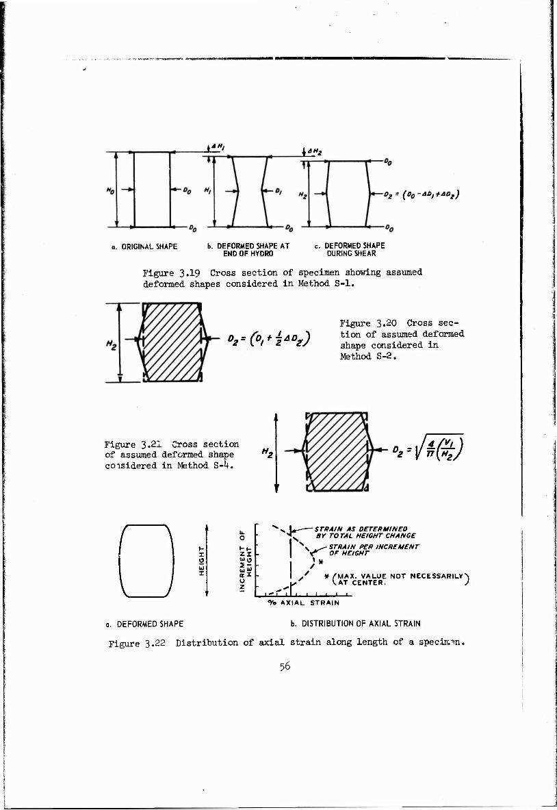
3.2.1 Method S-l. In this method, it is assumed that the axial

strain and the radial strain as calculated from the vertical displace-

ment of the top cap and the midheight radial deflection completely

represent the actual strains occurring within the specimen. Figure

3.19 shows the assumed deformed shape at the start of the shear test

and during the shear test. The deviator strain becomes

e - € = a r = Ho "I Do ) (3.23)

and the deviator stress is

35

nan<nat-iAia»K^ifi-r-r. ig Wliftmi' ,-,r.- |, M ,, y^ii, MflSKflMttWI j HWWWWWE HWI m.biniiWi.Trm —-II "».H

^^>mmii&m&^M

^\-:-^--^^^jtl^iiiiM&ȴii^^'^^^^^--ij^^^f:'-

Where:

D = current diameter during shear test

This method was used to calculate the deviator stress and strain re-

sults shown in Figures 2.3 and 2.U and will subsequently be referred

to in this paper as the "standard" method for comparison purposes.

3.2.2 Method S-2. For this method, assume that the axial de-

formation is representative, but that the center radial deformation

is a maximum value and therefore not representative of the entire

specimen. The radial deformation should therefore be weighted, and

for simplicity, an average value of one-half is used as shown in Fig-

ure 3«20, The deviator strain becomes

e - e a r = Ho "\f V

(3.25)

and the deviator stress is

o-a " °r - —; . " v2 (3.26)

4l + 2 *g)

Where: D1 = Deformed diameter at the end of the hydrostatic phase

3.2.3 Method S-3» In this method, it is assumed that only the

axial measurement is available and that the ratio of radial strain to

axial strain is equal to -O.5 in accordance with elastic theory for

pure shear. The deviator strain is therefore

0 \ o / 6a" €r = " " l-°-5^J (3.27)

36

-. .w ....>.^.,^JiaiAl,> -1-1- a 1 ■«^M^^wi^^^^^*.^■■n..-f.w aaaaa 1 i i 1' -niüiaüM—aniMtiiii'iiiii 'wikimtmrnummmr- müsämmäh- *-

wmmmm&mmm&&*9>!f*

and the deviator stress is

UP ar =

"M1 + I 6a) -^ J (3-28)

3.2.U Method S-U. This method is derived based on the assump-

tions that only the measured axial deformation is valid and that no

volume change occurs during the shear phase. This method is commonly

used in soil mechanics where only axial deflection is measured. The

specimen is assumed to undergo cylindrical deformation as shown in

Figure 3«21 with no change in volume. Because it is assumed that

there is no volume change during shear, the current diameter during

the shear test Dp can be expressed as

and the radial strain can be calculated as

(3.29)

e = r

D1"D2

vM) D (3.30)

Where:

V.. = deformed volume at the end of the hydrostatic phase

Hp = current height during shear phase

The deviator strain is therefore

r H D (3.31)

37

.-^„ns^^^Ä^iÄ^«^«^^*4«»** ** «

and the deviator stress is found from

Hfe °a - °r " ^ (3.32)

3.2.5 Method S-5. In this method, as in Method S-4, it is as-

sumed that there is no volume change, but in this case the axial de-

flection is assumed to be invalid so that only the radial deformation

is available for calculation purposes. The volume of the specimen,at

the end of the hydrostatic test V and the current diameter during

the shear phase Dp may be used to calculate an assumed current

height during the shear phase HJ!, for a right circular cylindrical

specimen, i.e.

wi - i?. 1 (u.vrt

2 o o 2

The axial and radial strains may be expressed as

H.-^ ^

e = a 1 * Do + 4 * DoD2

H o

. 3 r Do

The deviator strain is therefore

e - a

«I" 12 Vl

" Bo + 4 + DoD2 r H o ?)

38

(3.3^)

(3-35)

(3.36)

.Jr-bfe t:;-j, &£*& aw ■■ ju&amMtliÜää&BAWäA iHlii"iiniBi^ifci«8tta'^

memmm t^Kfifö^sKia

and the deviator stress is

a - a = a r

Up

fl(D2)' (3.37)

3.2.6 Method S-6. For this method, it is assumed that the axial

strain as calculated from the measured change in specimen height is

not representative of the axial strains within the specimen and that

the change in height measurement should be corrected by some empiri-

cal factor. An arbitrary factor of 2 is used for illustration pur-

poses. The deviator strain in this case is

e - e a r Ho \ Do I

(3.38)

and the deviator stress becomes

a - a = a r h?

n(D2r (3.39)

3.2.7 Summary. The above six methods represent various proce-

dures for calculating stress and strain in soil specimens during the

shear phase of triaxial tests. In Method S-l, stress and strain were

based on actual measurements of applied loads, displacement of the top

cap, and midheight diameter changes. Method S-2 was based on a repre-

sentative diameter as the average of a fixed end diameter and the meas-

ured diameter at the center of the specimen. Method S-3 is based on

an assumed strain ratio of -O.5 for elastic pure shear and the assump-

tion that only the axial deformation measurements are valid. For both

Methods S-k and S-5, it was assumed that no volume change occurs dur-

ing the shear phase. Method S-U required the use of only the axial

measurement for calculations; Method S-5 required only the use of the

radial measurement. Method S-6 was an attempt to correct the axial

39

•8-

unmeet®®*;*»*- ^ y^fefe^iia^ita; v^j^fe^,-;^,-.

BA -&w-i -ja; J-: ji\.-i**4Ej *.<. &a: wi*ii -.• ■ w«ei -a ?> '•?■ :*i£is. «.V.äw.Ai'ijiKA*«' J^*5.^^,^.i'Wy*AatJ~'iiA'-Ä.Vä-^ii-.iiii-j.^iiJ'ii. 'j*. &*täti^&iädtäb Kili*fcii«iA Jösäiiii

deformation by means of an arbitrary empirical factor based on limited

research conducted on the distribution of axial deformation of undis-

turbed specimens during the shear phase. In general, the greatest

axial strain seems to occur near the midheight of the specimen as il-

lustrated in Figure 3'22. All six methods discussed in this section

are summarized in Figure 3«23'

ko

1 1 r 1

u J

B I. DOUBLE CONE SHAPE

A B H CYLINDRICAL SHAPE

ORIGINAL SHAPE DEFORMED SHAPE

Figure 3.1 Deformed shapes of specimens during hydrostatic loading.

4l

I

■r.i ;i;,.j?„.-. ■.;r;HT^^*AV^^H-.^-'W'i^*J*:öi«^.-.v'-

:V'''1-- ^•■^^4-,m

tii^-i^'ji--^ ' JlTJii>lJi-.--,ii:j***.i'si J.

1.327" 1.313 it

\30l"

CO

%£9T% PI— « > •

/. 3/0"

\ 1.318" '

ORIGINAL DEFORMED

G"a = CTr = 500 PSI

o Figure 3.2 Triaxial specimen of recompacted clayey silt after being subjected to 500-psi hydrostatic pressure, shape IC.

k2

i nf nr iMiiamiJMiWir»ii anaaaüia H^anaaaaafeie^aü ■ jarittuaJMi

TOi^M«g^wir^u^«gyrr«w*»^^

1.327

3

11.327"

ORIGINAL

1.292*-

I.2SJ" 4

n

1.215" §

rg

A£5Q"

1 DEFORMED

C*a= 0^=5000 PSI

Figure 3o Triaxial specimen of reconrpacted clayey silt after bei™ subjected to 5,000-psi hydrostatic pressure, shape IC g

«•3

1.404" 1.392".

ORIGINAL DEFORMED

CTa = Up = 1000 PS!

o Figure 3.4 Triaxial specimen of a silty clay with rock fragments after "being subjected to 1,000-psi hydrostatic pressure, shape HA.

kk

tnyyn»».iT~"-' *~ ■- .--

1.388"

J 1.368"

ORIGINAL D rORMED

C"a = CTr = 5000 PSI

Figure 3.5 Triaxial specimen of siltv ,-lav with ™„v r being subjecte«! to 5,000-p5i ^Jl^Z^^lZ^^ "«• pressure, shape HA.

U5

"*—Dr +—D«

a. DEFORMED SHAPE b. ASSUMED DEFORMED c. DOUBLE CONE SHAPE

Figure 3.6 Cross section of shapes considered in Method V-l.

Ht D0-2A°I

Figure 3*7 Cross section of assumed shape used in Method V-2.

Figure 3.8 Cross sec- tion of assumed shape used in Method V-3.

-DEAD ZONE

CYLINDER SHAPE CONSIDERED

a. CROSS SECTION b. ISOMETRIC

k6

Figure 3-9 Assumed shape used in Method V-^.

wmmm mm m l!«i»^*^

P 0) O

H 1 •d Co P Ö +> <d CD I •H

to •H CD

Si § • CD CO

CO cd

Ü Mi-I -Ö ^r JO a) fi cd firjfi

■H CO CO CD p £>

•H O fi to 9\

DO -P <H p +> -p p> *\ R i-l B> O H i-l CO s H

•H P H -d •ri 3 H P iH CD P (0 co 0) C -P to 03 ^ § p O p CD -P V cd 0> pi CD 3 c , f>>

H 0) fi N a« 2 Pi d ■£ fcj IV

p 3 o) H V J3i?p -p p o

Pi O >> •P Ä > p >> S 2 5* •H S S

CH ,O to CD CU -H

to +3 i-(

CD H g o

fi J3 i CD -P

to to -P O T) H p, H cd CD CD Ö ^ X at 0) CH 0) H CD CD Ö £5 p p u V ß co a> -p MAO) Ot) TI to -H a P co M O -d P CD -P -P X P M

CD >H -H to cd cd

1 O -P o ä p cu -P CD cd P CD U o p fH > 3 6 P » fi

CD M 3 -P CO >j O CD TH fi « fi -p

11 TJ a> <u M O CD iH P J ° -. H H Pi M pi -P <d CD > CD H -P cd H

e u r-4 cd H ca CD CD g H JP cd to •H H

k 3 O CO ai r<3 cd cd Ti to H a>

,P fi CD 8 -P 8 to M

•b CD -p •H

Sä •d cd

CH cd •d fi •nop .p P fi H CO * CD CD cd H o S-d .c to -P CD O cd ■Ö g SH cd .a !H H ü cd £«M v fi CD O

O -P « P CD CD S <H X! co X! -H P H •d -H -p O -P H fi 2 _ -p +3 -p o cd

ü g, h q e M«d cu cu

a) CD '« i-l >d M

to p "Ö cd -P cu

to CH cd

■d -H cd ß cu o O p C CD +3 O -P O H CD CO H -H 5

<U H -P CO O iH -P CU CU Ü to CD

3£ CD H iH p fi "d cd CD cd CD > >> CD J3 to cd >» CD m -ri u co H to P

ffl p. < t< ,Q -P D o b o CQ tO -P J3 CD |3 O

H~ cd *^-\ *"-N ^•~v Ul cd H l-l 1 1

Ul

fel o 1 I cd

H i

^|> cd ID

cd ui

N—^ H

*—* *—' CM fH OJ M <H Ul Ul CM >H O «V^ w^k + r-i|ro

Ul

p <M|ro o + + cd 1 •H IU + -P cd cd u h cd U> CD Ul Ul cd H M H C\J cd Ul p Ul CD Ul u O 1 Ul H i 1 1

CD ^ + U M u ui ,,fn

Ul Ul OJ Ul Ul

+ + + + 1 ai h

! cd cd CO cd Ul Ul Ul U) w Ul H oo m

■d O

-P

H CJ on _. iTv vo

1 > > 1 > 2 > ji £

U7

SHEAR TYPE I

SHEAR TYPE I ORIGINAL SHAPE DEFORMED SHAPE

Figure 3-H Shapes of failed specimens after shear test.

'48

a. Specimen as removed from test device.

b. Specimen separated to show shear plane.

Figure 3.12 Triaxial specimen of sandstone after shear failure during a dynamic constant p-type test, shape HA.

^9

ORIGINAL DEFORMED

C7r = 5000PSI

CTa=5000 PSI + SMALT LOADING INCREMENT-

A3307

Figure 3.13 Triaxial specimen of recompacted clayey silt after being subjected to a small deviator stress while maintaining a confining pressure of 5>000 psi.

50

i

ORIGINAL

ORIGINAL SHAPE

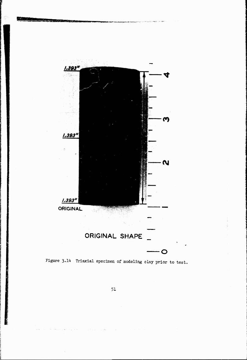
Figure 3.14 Triaxial specimen of modeling clay prior to test.

51

1.389 I.3Z2?

ORIGINAL DEFORMED

CTr = 5000 PSI _

0^=5000 PSI + LOAD INCREMENT I

Figure 3-15 Triaxial specimen of modeling clay after ap- plication of a small deyiator stress while a confining pressure of 5,000 psi is maintained.

52

^rrr^f^^mv^^m^r^' «JCffSSg??*^

1.393"

ORIGINAL DEFORMED

crr = 5000 psi -

CTa = 5000 PSI + LOAD INCREMENT 2

Figure 3.16 Triaxial specimen of modeling clay after ap- plication of a larger deviator stress vhile a confining pressure of 5,000 psi is maintained.

53

mmm wmmnmaem

/.W /.*$<?"

B— <\i

f\J

WL&O"

B— 4ä*" 1 >

ORIGINAL DEFORMED

C7r=5000 PSI _

CTa=5000 PSI + LOAD INCREMENT 3

Figure 3»17 Triaxial specimen of modeling clay after ap- plication of large (postyield) deviator stress while a confining pressure of 5,000 psi is maintained.

5^

■BJ^-j^. ■--&?**?^35*' ^■**•-"■

A ORIGINAL

SHAPE

D LARGER

INCREMENT OF LOADING

END OF HYDROSTATIC

TEST

START OF SHEAR TEST WITH SMALL AXIAL LOADING

AT OR NEAR YIELD STRENGTH

POSTYIELD

Figure 3-18 Specimen deformation during shear test,

55

k*»l kl?2

°2= (D0-^O,+A0g)

a. ORIGINAL SHAPE b. DEFORMED SHAPE AT END OF HYDRO

c. DEFORMED SHAPE DURING SHEAR

Figure 3.19 Cross section of specimen showing assumed deformed shapes considered in Method S-l.

°Mm(Di*i*°t)

Figure 3.20 Cross sec- tion of assumed deformed shape considered in Method S-2.

Figure 3«21 Cross section of assumed deformed shape coisidered in Method S-h.

■i/*£j

o. DEFORMED SHAPE

O

ZX w O

ll O z

-STRAIN AS DETERMlNED BY TO TAL HEIGHT CHANGE

STRAIN PER INCREMENT OF HEIGHT

* /'MAX. VALUE NOT NECESSARILY"

1 I I L.

.AT CENTER.

-t- % AXIAL STRAIN

b. DISTRIBUTION OF AXIAL STRAIN

Figure 3.22 Distribution of axial strain along length of a specimen.

56

Method Calculation of {a - a) and (e - e ) Rejnarks

S-l

S-2

s-3

S-U

s-5

S-6

UP

"(D2)2

füg /^\ Ho VDo/

4P

C. - 6_ »

a - a =

e_ - *_ =

O - <7_ =

n(D1 + I AD2)2

Ho 'V Do>/

jtf "[00(1 + | e

a) " AD1]2

AH / ^2\

v7~

AH-, *-J3 a - c = J*P_

n(P2)2

12 1 " D2 , „2

«_ - e_ = ' o + D2 * DcD2 /^\

a - a = • 4P

n(D2)'

= 2 AHg /-A^\

Ho ~\»o )

Use of actual measurements, cross-sectional area based on center diameter

Radial deformation averaged, resulting in a smaller diameter than that of the center measured diameter

Based on theory of elasticity, where it is assumed that there is no volume change during pure shear and that er/ea = -0-5 • Use of only the axial measurement

Assumed that there is no volume change; axial measurements used to calculate diameter

Same as S-k except radial measurements used to calculate height

Arbitrary correction of axial deformation to reflect greater center strain

Figure 3.23 Summary of methods used to calculate deviator stress and strain.

57

■'" ~s^"^&!mai*mmjw«umam

CHAPTER k

DISCUSSION OF INTERPRETATION METHODS

As described in Chapter 3» various methods can be used to calcu-

late stress and strain from load and deformation measurements obtained

during triaxial tests. The differences between each method can prob-

ably best be illustrated by stress-strain curves calculated from raw

test data obtained from two extremely different undisturbed specimens,

i.e. one quite soft and one very stiff. The soft specimen, the sandy

clay previously described in Figure 2.3, was subjected to a hydrostatic

loading of 1,000 psi and then carried to failure in shear while the

mean normal stress remained constant. The stiff specimen, the silt-

stone previously described in Figure 2.k, was subjected to a hydro-

static loading of 1,500 psi and then carried to failure in shear while

the confining pressure was held constant. Measurements made for both

tests included confining pressure, axial load, change in height, and

change in midheight diameter. A double-cone deformed shape best ap-

proximated the response of both specimens during the hydrostatic test,

followed by a bulging shape during the shear test. Both specimens

formed shear planes at failure. As previously mentioned, Method V-l

for the hydrostatic test and Method S-l for the shear test will be

considered as the standard analysis methods for purposes of comparison.

k.l COMPARISON FOR HYDROSTATIC TESTS

Pressure-volumetric strain plots for the sandy clay specimen dur-

ing the hydrostatic loading test are shown in Figure k.l for each of

the six methods previously described for calculation of voludietric

strain. Values of volumetric strain and approximate bulk moduli K ,

calculated for both the 0- to 100-psi and the 600- to 1,000-psi pres-

sure ranges, are also included in Figure k.l. Method V-2 yielded

58

■!f-ima'.^ri-'s';«*,'--. "■■:

essentially the same strain values as the standard Method V-l, because

of the equality of the two methods except in small-order terms.

Method Y-k resulted in only slightly greater volumetric strain; i.e.

the difference between this method and the standard is unnoticeabl'i

on the plots for volumetric strains less than 5 percent, which is

reasonable to expect since the dead zone considered in the calculation

was very small compared to the large original volume. Methods V-6,

V-3, and V-5 gave substantially larger strains than did the standard

method. At lower pressures (less than 100 psi), these three methods

are in close agreement with strains exceeding the standard by approxi-

mately 50 percent. At higher pressures, i.e. 1,000 psi, Method V-5

gave the largest strain, exceeding the standard by approximately 65

percent. Methods V-6 and V-3 showed fairly close agreement, exceeding

the standard strain at ,1,000 psi by about k$ percent. It should be

noted that since the deformation results are material-response depen-

dent, the same percentage difference may not hold for different ma-

terials. In fact, similar calculations by WES using other test data

resulted in Method V-6 giving the largest volumetric strain values;

however, Methods V-l, V-2, and V-k will probably always give smaller

volumetric strains than Methods V-3, V-5, and V-6.

Comparison of bulk moduli values for the pressure range of 0 to

100 psi shows that the maximum bulk modulus was calculated from Method

V-l. The lowest modulus, calculated from Method V-6, was 35 percent

less than the standard. Values of bulk moduli for the high pressure

range, 600 to 1,000 psi, varied from 57 percent less than to 21 per-

cent greater than the standard. The lowest modulus was calculated by

Method V-5 and the greatest modulus by Method V-6. Again because of

the dependence of the deformations on material-response behavior,

there are no fixed relations between methods.

The same basic trends observed for the relatively soft sandy

59

.^sV&V^V*^ i^tf*?*)8»SsSa*>J*

clay specimen are apparent in the pressure-volumetric strain plots

for the relatively stiff siltstone specimen as shown in Figure k.2.

Methods V-l, V-2, and V»k gave essentially the same volumetric strain

results. Again Methods ~'~3, V-5, and V-6 gave substantially larger

strains ranging from kO percent (Method V-6) to 63 percent (Method

V-5) greater than the standard at a pressure of 1,500 psi. At a pres-

sure of 200 psi, the volumetric strain calculated by Method V-5 was

110 percent greater than that calculated by the standard method. Note

also that, while Method V-6 gave larger strains at high pressure, it

gave lower strain values than the standard method in the low pressure

range.

The bulk moduli values varied from a low of k2 percent less than

that calculated from the standard at low pressures (200 to 600 psi) to

U5 percent less thai the standard at high pressures (l,200 to 1,500

psi). Method V-5 gave the lowest modulus for the low pressure range

while Method V-6 gave the lowest value for the high pressure range.

At the low pressure range, the bulk modulus as calculated from Method

V-6 compared favorably with the standard.

From the two above examples, several rather general observations

can be made regarding the comparison of methods to calculate volu-

metric strain. First, the results indicate that the volumetric

strains are different at any given pressure when calculated by Meth-

ods V-5 and V-6. Both methods are based on the theory of elasticity,

which assumes for hydrostatic compression that axial and radial

strains are equal; one method used only axial strains and the other

only radial strains to calculate volumetric strains. Obviously the

axial and radial strains as derived from the axial and radial defor-

mations of the specimens were not equal nor were the specimens

elastic.

Far from being elastic solids, soil specimens are in fact

60

»a SBgyfSS^sVf^Xff^W"^'^':'

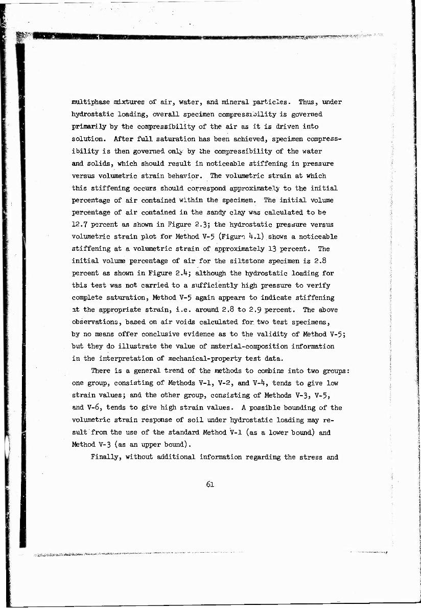
multiphase mixtures of air, water, and mineral particles. Thus, under

hydrostatic loading, overall specimen compressuility is governed

primarily by the compressibility of the air as it is driven into

solution. After full saturation has been achieved, specimen compress-

ibility is then governed onlv by the compressibility of the water

and solids, which should result in noticeable stiffening in pressure

versus volumetric strain behavior. The volumetric strain at which

this stiffening occurs should correspond approximately to the initial

percentage of air contained within the specimen. The initial volume

percentage of air contained in the sandy clay was calculated to be

12.7 percent as shown in Figure 2.3; the hydrostatic pressure versus

volumetric strain plot for Method V-5 (Figure k.l) shows a noticeable

stiffening at a volumetric strain of approximately 13 percent. The

initial volume percentage of air for the siltstone specimen is 2.8

percent as shown in Figure 2.k; although the hydrostatic loading for

this test was not carried to a sufficiently high pressure to verify

complete saturation, Method V-5 again appears to indicate stiffening

at the appropriate strain, i.e. around 2.8 to 2.9 percent. The above

observations, based on air voids calculated for two test specimens,

by no means offer conclusive evidence as to the validity of Method V-5;

but they do illustrate the value of material-composition information

in the interpretation of mechanical-property test data.

There is a general trend of the methods to combine into two groups:

one group, consisting of Methods V-l, V-2, and V-U, tends to give low

strain values; and the other group, consisting of Methods V-3, V-55

and V-6, tends to give high strain values. A possible bounding of the

volumetric strain response of soil under hydrostatic loading may re-

sult from the use of the standard Method V-l (as a lower bound) and

Method V-3 (as an upper bound).

Finally, without additional information regarding the stress and

61

srjjSitfäÄÄ*«**»*««^

strain distribution within each specific triaxial specimen, there

appears to be no reason why the standard Method V-l, based on actual

measurereants, should not continue to be used to develop plots for

data presentation, but the results from this method should not be

used in constitutive property analyses without due consideration of

the possible errors involved.

k.2 COMPARISON FOR SHEAR TESTS

Deviator stress versus deviator strain plots for the sandy clay

specimen during the shear phase of the test are shown in Figure 4.3

for each of the six methods previously described for calculation of

deviator stress and strain. A table listing the deviator strains and

approximate shear moduli for two deviator stress ranges is included

in the same figure; Method S-l will be considered the standard for

comparison purposes. Note first the similarity between all the curves

and the relatively tight data band produced by Methods S-l, S-2, S-3,

and S-k. Considering the deviator stress at a deviator strain of it-

percent as an indication of ultimate yield strength, the results for

all six methods only ranged from a high of 8 percent greater (Method

ii-5) to a low of 7 percent less (Method S-6) than that given by the

standard method. The shear moduli values calculated for the higher

deviator stress range (100 to 150 psi) tend to show more scatter,

however. The maximum shear modulus in this pressure range as calcu-

lated by Method S-5 was 29 percent greater than the standard of 2,300

psi and the lowest shear modulus by Method S-6 was 35 percent less

than the standard.

The variation in initial shear moduli data can best be seen in

Figure k.k, which is an enlarged view of the initial portion of the

deviator stress-strain curves presented in Figure 4.3. Although there

is a more noticeable deviation from the standard by Methods S-5 and

62

.K-:-*V< F tfwawwitaiti**!»)

mmmmg*mmm$mmam-mMm&*&l£^

S-6, the tighb banding of Methods S-l, S-2, S-3, and S-k is still evi-

dent. The range of shear moduli for the 0- to 70-psi pressure range

varied from a high of 115 percent greater than the standard for

Method S-5 to a low of k8 percent less than the standard for Method

S-6. The deviator stresses compared at 1 percent deviator strain

ranged from 16 percent greater than the standard to a low of 19 per-

cent less than the standard value.

The deviator stress-deviator strain plot for the shear phase of

the siltstone test is shown in Figure k.'y. Although the curves tend

to produce the same general trend, the values as calculated by Methods

S-l, S-2, S-3} and S-k are not as close as in the sandy clay example.

The deviator stress values taken at 0.6 percent deviator strain as

an indication of ultimate yield strength range from a high of 23 per-

cent greater to a low of 21 percent less than the comparable deviator

stress value from the standard method. The yield strength is not

shown in Figure 4.5, but based on calculations for the complete shear

test data, the maximum yield strength is approximately the same value

for all methods although the corresponding deviator strain values

range from kO percent less than to 100 percent greater than the devi-

ator strain value of 1.5 percent calculated at maximum deviator stress

by the standard method. The shear moduli values taken at high devia-

tor stress levels (to) to 600 psi) vary from a high of 51 percent

greater than the standard for Method S-5 to a low of 33 percent less

than the standard for Method S-6. The shear moduli values taken at

the medium deviator stress range (200 to UOO psi) vary from k2 percent

greater than to 38 percent less than the values calculated by the

standard method.

An expanded view cf the initial portion of the deviator stress-

deviator strain plot for the siltstone test is shown in Figure k.6.

The curves for this particular test, however, were based primarily

63

E&8»Ä.^l^^wt*;* ^"*-> .'••'«-^

on extrapolation of data measured at higher stress levels; and, al-

though other test data have shown that the various calculation methods

do affect the initial portion of the shear results, use of these par-

ticular data will only demonstrate possible variations. The standard

method gives the minimum numerical value of deviator strain for any

given deviator stress level, while Method S-6 still gives the maximum

numerical value of deviator strain. Method S-5 yields the second

highest value of deviator strain up to approximately 200-psi deviator

stress. Methods S-2 and S-3 give similar results. The shear moduli

values in the 0- to 100-psi stress range decrease in value from the

standard of 555,000 psi to a minimum of 167,000 psi as calculated by

Method S-6.

Several observations can be made based on the calculated stress-

strain res alts shown for the two shear test examples. In general,

all the calculation methods will give approximately the same values

for maximum yield strength, but significantly different values for

the deviator strain at which maximum yield strength occurs. Methods

S-l, S-2, S-3, and S-^l appear to give approximately the same overall

stress-strain results with their curves bounded from above by the

stress-strain curve calculated by Method S-5 and from below by the

curve calculated by Method S-6. Bounding for the initial shear

modulus does not appear feasible as yet since, at low deviator stress

values, any of the methods could yield the maximum shear modulus ex-

cept Method S-6, which appears to give the lowest values of shear

modulus regardless of material type. Method S-6, however, was based

on an arbitrary correction of axial deformation and the results with

this method therefore can only be considered as an illustration.

Basically the standard method, S-l, is considered satisfactory

at this time for the calculation of deviator stress and deviator

strain from laboratory load and deformation measurements since it

6U

does tend to produce an average of the stress-strain results as

calculated from the other five methods.

Although triaxial test results are seldom, if ever, presented in

terms of deviator stress versus volumetric strain, comparison of such

plots based on the various stress and strain calculation methods

previously described may be beneficial in view of recent interest

by developers of constitutive models in the volume change characteris-

tics of soils and rocks during shear. Results for the siltstone ex-

ample test are presented in Figure 4.7» It is realized that there is

some question regarding the proper usage of Methods V-5 and V-6 to

calculate volumetric strain during the shear phase of the test; how-

ever, the calculated results do illustrate trends. The values of

deviator stress were calculated for all six volumetric strain calcu-

lation cases by Method S-lj volumetric strains were not rezeroed at

the start of the shear phase, but v.rere continued from the last point

which occurred during the hydrostatic phase.

Methods V-l. V-2, and V-k show initial volume increase followed

by a volume decrease t) failure. Method V-3 shows an initial volume

increase followed by little change in volumetric strain to peak devi-

ator stress. Method V-5 shows little initial volume change followed

by an increasing rate of decreasing volume. Method V-6 shows a rela-

tively constant rate of increasing volume change followed by a rapid

increase near peak stress.

The principal observation that can be made based on the results

shown in this example is that any conclusions made from triaxial test

results as to whether dilation, compaction, or no volume change occurs

or does not occur during shear of a given material may be completely

masked by the particular method of data analysis chosen by the

experimenter.

65

I SäW#!»l**!^%^«feHMi».^^ . ■'■T'.^VCV"-^;.:

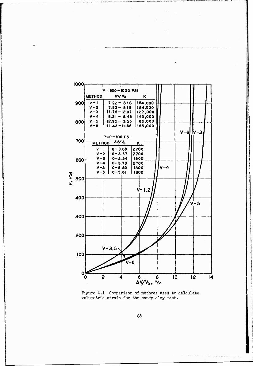
1000

900

800

700

600

Q- 500 Q.

400

300

200

100

1 1 1 1 P = 600 -1000 PSI METHOD AV/Vo K

V-l V-2 V-3 V-4 V-5 V-6

7.92- 8.18 1 7.93- 6.19 1

11.75-12.07 1 8.21 - 8.48 1 12.95-13.55 11.43-11.65

P = 0-IOO PSI

54,000 ■ 54,000 22,000 45,000 66,000. 85,000

V-6 V-3|

METHOD av/v0 K

V-l V-2 V-3

0-3.66 0-3.67 0-5.54

2700 1 2700 1 1600 1

V-<

V-«

% i

0-3 0-5 0-5

73 52 61

27 18 18

00 f 00 / 00 /

'v-4

/

\ '~1,2//

/

//v '-5

\ /-3,5N

^V-6

6 8 AV/V0,«/o

10 14

Figure k.l Comparison of methods used to calculate volumetric strain for the sandy clay test.

66

I.IIU.I 1 ■ I. IIW|. | UIH.^il.HI.I.» *m*mmmm*mmmm*^m

1600

P=200-600 PSI METHOD AV/V0 K

V-1,2,4 V-3 V-5 V-6

0.42-0.88 10.54- 1.20 [0.88- 1.68 1038-0.88

87,000 61,000 50,000 80,000

1200-1500 PSI AV/V0 K

152-1.72 2.20-2.54 2.19-2.80 2.06-2.42

150,000 88,000 97,000 r~ "»00

Figure k.2 Comparison of methods used to calculate volumetric strain for the siltstone test.

67

v,,,w —.1 Mj■ HpppjinyiwppmJI i - — —wmm 11, mmmvpmmm* www ;*'-■• •■*A-*i^ft*ffij^>w wggywpw* iw J.'JBJUKWWWPW'J^"1 " ■

o

o «

go o h-

- i o «■ w

\\\

2,3

00

2,

500

2,50

0 2

,30

0

•a A

nn

>o >o w to

~ 0J0J 1—

i i i i i ^oooo

ÖOOÖC

ooooc ooooc ooooc M » * « — oo« 0

1 11 </>

JO

>—

>o I 1 \\\ >o >o

J

W \ TO

v\ ' \

iO<DT

d dddc i i i i i o oooc

tat -m >d

i >o j \1

ftl \

i i i i i 1

IV)

i

o •0

m * 03

CO

-P

o CO

* o -p cd

•H >

ui ■8 CO

-p

pi o Ü

CO >5 H CO • ü -P

O d)

L +3 -P

«0 (VI <D cd

CO H 0 3 Ü vw

CO >5 V»-' ■d #

o o ß Xi cö

04 +3 W <u g Jj

.ß <M -P o

(0 ß o O <H CO

•H ß IH -H cd cd

o O CO Ü

o OO -P

• cd

m ü

•H ß &4 cd

O O O O o o o »0 O •n O «0 o in CO ro (VJ <M mm

ISd '(JD-°D)

68

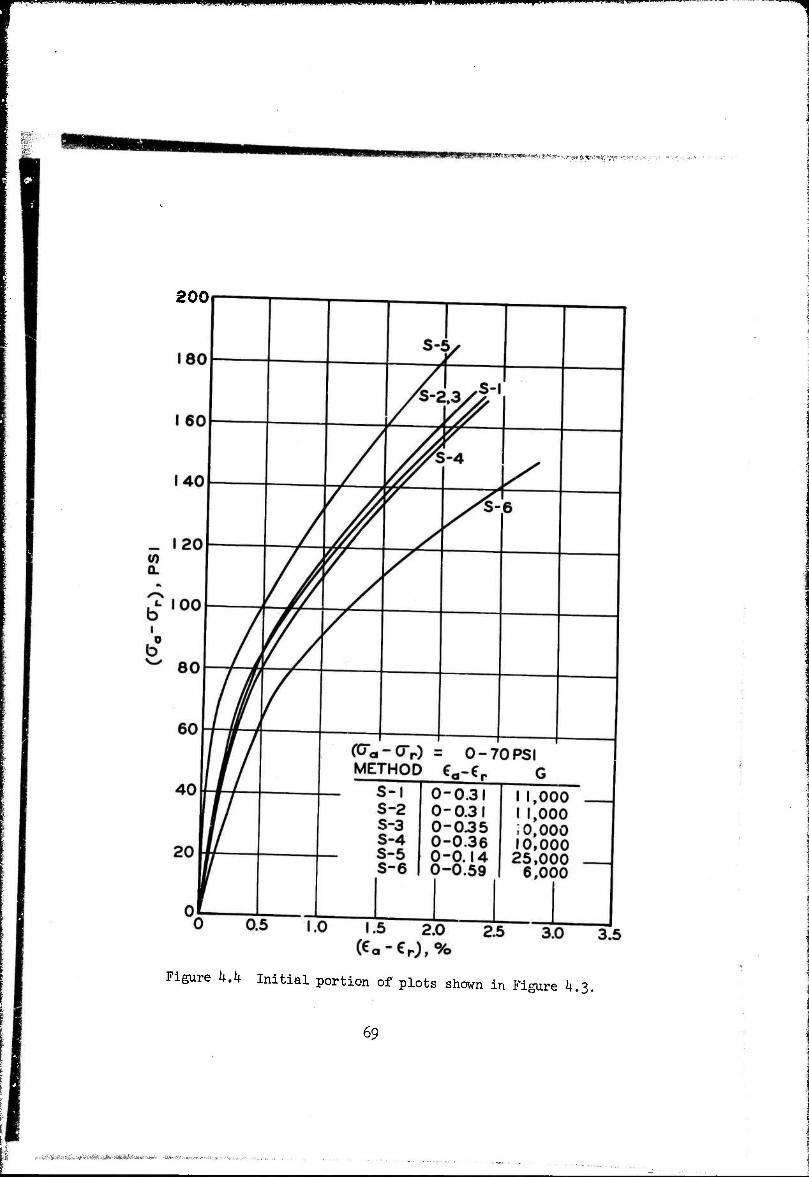
-*—-•• • ™in^c^mi^m*mmmmmimmm*im i in ■

&X&?:$i!*?BsF'-7-~>F&?*F'~-.*:?*fkK'~-n-f V'W '•"'■**■' -*

200

Figure k.h Initial portion of plots shown in Figure k.3>-

69

. ',1* 1 U - .,. v - j. ' * j*fc Jtt^s^wfcw*

i. mt"i*J-.'Kixn* wn mPFVtnmwin^Hn^F ■-«"

>,^y?^e^y»^^y*^

2 o o ? - O 0

oooooo oooooo oooooo PJO(VI *On- at ^•TW^-tfXVl

(OOXSOXVIf) *(«>**(*> h-

^" • ■ • # •

oooooo 1 1 1 1 1 1

(VI—<V|N—«*) odd odd

i0 i

</)

■ l it

«jo Q. O O

1 (- o w

o 0 (VI yj

5) O 0. o o

° '» „ w

oooooo oooooo oqoqqq -T-TroOh"©

i CO

lOh-'O ^"COO

\

(Vl\ \\

Po>io h-r-co (vi =: (vi (vi -co

556,0

00|

0.0

3-C

250,0

001

0.

05-C

2

63

,00

0»

0.

06-<

455,0

001

0.0

6-<

192,0

001

0.

06-1

1

67

,00

01

0.I2-«

VA* •v \v V°

(0 V i

A

0-

0.0

1 0-

0.0

2 0-

0.0

2 0-0

.0 1

0- 0

.03

0- 0

.03

gin — (vi m ^ in <o i i i i • i

</)</)</> O (/) </)

o» d

00 ö

d

o o o

#

ow I 0

d

d

(M d

8 CO

o o (0

o o

o o (VI

Cd w

-p CO

u o -p cd

•H !> <D -d 0) -p CO

o H CO a o -p

-p w <u -p

a> a) a o -p

CQ W

O H

-p CQ CD S <»

Ä

Ö P O <+-•

•So ft ^ ö W Ü

fn O

LA -P • CO

cu a>

5o' •H Ö

ISd <(JJO-°JO)

70

J»iw '-'. ■ ■■»■W^IPWinWff^^^f ■m mill wmmnammsz^i^imß

mwmwj<iwwv*mw!iiJiHiWrXr3*'*asf"¥%--'t^

(0 Q.

b i

200

180

160

140

120

100

80

60

40

20

s-iy /S-2/ ws~3

s-4/yÄ 5-5 > /^-6

(<

METH OD €0

0-100 PSI

G S-I S-2 S-3

0-0.009 i 0-0.020 ; 0-0.019 Z

556,00C »50,0 OC >63,00C *55,00C 92,00C 67,00C

) ) )

0 «

S-i

t

5 3

0-< 0-(

3.026 3.030

> >

0.05 0.10 (CQ-€r),%

0.15

Figure k.6 Initial portion of plots shown in Figure h.5 (based on extrapolation of test data).

71

r i^^,-''.^f^w^^^piy^"wwg"WPF"^^^^--'*w'- ■ wmsmt

\

\ 1

c\ • >

(V

1 >

1 /

<0

(VI

CO

(I)

$

(VI (vi

oo

o o o

o o oo

o o <0

o o o (VJ

<0

CO u p to

o •H u p

H

o

o -p

Tf <D 03

CO T) O

P 0) S

o

c o p W P H ■H CO Ö

O CO

•H JH CO

g °

ID Ä P

Ü

cd d)

w

0) bo

•H 2

ISd '(JD-Di))

72

mmtmmmr mmmmm

j^aBgÜBW !M«yt"-'!".' ''*" w*

CHAPTER 5

CONCLUSION

The purpose of this paper was to show with specific examples the

possible influence exerted due to interpretation of raw load and de-

formation data on the stress-strain relations obtained from labora-

tory tests. The triaxial test was selected for illustration purposes,

and observations were made regarding physical response of typical

specimens subjected to both hydrostatic loading and shear loading.

Six methods to calculate volumetric strain and deviator stress and

strain were derived based on a variety of empirical and theoretical

approaches and applied to calculate stress-strain relations for two

widely different materials.

Results of the hydrostatic phase calculations indicated that vol-

umetric strains were generally bound by Methods V-l (lowest values)

and V-3 (highest values); the actual hydrostatic stress-volumetric

strain response of a given soil or rock material probably lies within

those bounds. Results from the shear phase calculations indicated

that the use of Method S-l to calculate the overall deviator stress-

deviator strain curve is probably satisfactory; however, selection of

an initial value for shear modulus must depend to a great degree on

the compatibility with moduli observed from tests conducted under

other states of stress.

Research is under way to develop improved measurement systems

which attempt to circumvent the important influence of imposed bound-

ary condition on the specimen's stress-strain behavior. Finite ele-

ment analyses of laboratory tests are also under way to provide some

insight into the degree of influence of boundary conditions on the

distribution of stress and strain within the specimen and possibly to

disclose procedures for relating externally measured loads and

73

■'■».V»jp»^ljl iw,lj>ijPjpjUmi.j.

deformations to the most representative stress-strain behavior of a

given test specimen. Until the results of such research are avail-

able, continued use of the standard mechods, i.e. Method V-l for

volumetric strain and Method S-l for deviator stress and strain, to

develop plates for triaxial test data presentation appears justified.

Code developers can provide very useful information to experi-

menters through their ability to conduct controlled parameter studies

of the influence of material properties in ground shock calculation;

results from such studies can enable the experimenter to concentrate

his research efforts on those properties having the greatest influence

on wave propagation through earth materials. There are certain favor-

ite areas that experimenters like to investigate which may or may not

have any influence on the propagation of ground shock while other

overlooked areas might be of prime importance.

Hopefully, through a coordinated research effort, such as the

DASA-sponsored program at WES, significant results will be attained

for use not only in the specific area of constitutive model formula-

tion for ground shock codes, but also for broad application in the

general field of soil and rock mechanics.

71*

•n*n»lp<«pHMKy*«!ian«"B^ IJlliLI I. Ill 1 111 ■JJPM!« .I-..IIIIIHI ■. '■ ^

MMBBWMW»*!1«!»'*^^

REFERENCES

1. G. F. Sowers; "Strength Testing of Soils, Laboratory Shear

Testing of Soils"; ASTM Special Technical Publication No. 361, 1964,

Pages 3-5, 9-l4; Unclassified.

2. A. W. Bishop and D. V. Henkel; "The Measurement of Soil Prop-

erties in the Triaxial Test"; Second Edition, 1962; Edward Arnold,

London; Unclassified.

3. W. G. Shockley and R. G. Ahlvin; "Non-Uniform Conditions in

Triaxial Test Specimens"; Research Conference on Shear Strength of

Cohesive Soils, i960, Page 34l; American Society of Civil Engineers,

Boulder, Colorado; Unclassified.

4. "Strain Variation in a Triaxial Soil Test"; Technical Docu-

mentary Report No. AFWL TDR-64-47, September 1964, Pages 17-l8; IIT

Research Institute for U. S. Air Force Weapons Laboratory, Research

and Technology Division, Contract AF 29(60l)-6004; Unclassified.

5. B. B. Mazanti and C. N. Holland; "Study of Soil Behavior

Under High Pressure"; Contract Report S-70-2, Report 1, Vol. 1,

February 1970; U. S. Army Engineer Waterways Experiment Station, CE,

Vicksburg, Miss.; Unclassified.

6. J. M. Duncan and P. Dunlop; "The Significance of Cap and

Base Restraint"; Journal of the Soil Mechanics and Foundations Divi-

sion, January 1968, Vol. 94, No. SMI, Pages 271-289; American Society

of Civil Engineers; Unclassified.

7. P. W. Rowe and L. Barden; "importance of Free Ends in Tri-

axial Testing"; Journal of the Soil Mechanics and Foundations Divi-

sion, January 1964, Vol. 90, SMI, Proc Paper No. 3753, Pages 1-27;

American Society of Civil Engineers; Unclassified.

75

t^|ffijffi|flfl^