Embed Size (px)
Citation preview
Self-assembly of Donor-acceptor Conjugated Polymers Induced by Miscible ‘Poor’ Solvents
Yuyin Xi, Caitlyn M. Wolf and Lilo D. Pozzo*
Department of Chemical Engineering, University of Washington, Seattle, WA 98195
Email: [email protected]
Supporting Information
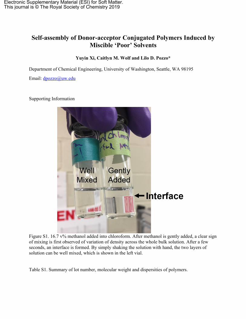
Figure S1. 16.7 v% methanol added into chloroform. After methanol is gently added, a clear sign of mixing is first observed of variation of density across the whole bulk solution. After a few seconds, an interface is formed. By simply shaking the solution with hand, the two layers of solution can be well mixed, which is shown in the left vial.
Table S1. Summary of lot number, molecular weight and dispersities of polymers.
Electronic Supplementary Material (ESI) for Soft Matter.This journal is © The Royal Society of Chemistry 2019

Polymers Lot # Mw Ð
DPPDTT M315 279 k 3.65
PCDTPT YY9100 & YY11066 76 k 2.5
PFT-100 YY8224P1 50 k 3
PCDTBT MKBJ8073V 52 k 5.38
Figure S2. AFM images of 1.6 mg/ml DPPDTT in chloroform mixed with (a) (b) (c) (d) 10 v% methanol and (e) (f) (g) (h) 20 v% methanol after aging for (a) (e) 2 hrs, (b) (f) 3 days, (c) (g) 6 days, (d) (h) 12 days.
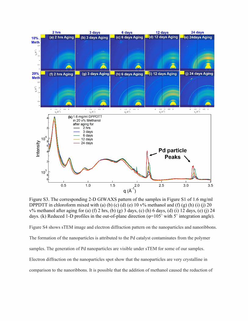
Figure S3. The corresponding 2-D GIWAXS pattern of the samples in Figure S1 of 1.6 mg/ml DPPDTT in chloroform mixed with (a) (b) (c) (d) (e) 10 v% methanol and (f) (g) (h) (i) (j) 20 v% methanol after aging for (a) (f) 2 hrs, (b) (g) 3 days, (c) (h) 6 days, (d) (i) 12 days, (e) (j) 24 days. (k) Reduced 1-D profiles in the out-of-plane direction (φ=105˚ with 5˚ integration angle).
Figure S4 shows sTEM image and electron diffraction pattern on the nanoparticles and nanoribbons.
The formation of the nanoparticles is attributed to the Pd catalyst contaminates from the polymer
samples. The generation of Pd nanoparticles are visible under sTEM for some of our samples.
Electron diffraction on the nanoparticles spot show that the nanoparticles are very crystalline in
comparison to the nanoribbons. It is possible that the addition of methanol caused the reduction of

residual catalyst leading to the formation of Pd nanoparticles. The (110) face of Pd crystal matches
with the peak at q=2.2 Å-1 and (200) face corresponds to the peak at q=3.2 Å-1.
Although Pd nanoparticles exhibit well-defined peaks at high q-range, no evidence that palladium
particles affect or interference with the low-q scattering data (SANS and low-q GIWAXS) from
polymers was noticed. In GIWAXS data, only the high-q peaks at q=2.2 Å-1 and 3.2 Å-1 grow
with aging when methanol is added (Figure S3) and nanoparticles are formed. All the other
polymer peaks and features stay the same as a function of aging. This indicates that the
generation of Pd particles does not alter the polymer peaks. With respect to SANS experiments,
the neutron scattering contrast between the hydrogenated polymer molecules and the deuterated
chloroform is about one order of magnitude larger than that between palladium particles and the
solvent. Moreover, the much larger size of the polymer structures that are formed (i.e.
micrometers long), as compared to the Pd nanoparticles (~10 nm), leads to total dominance of
the scattering at very low angles (SANS region) by the conjugated polymer.
Figure S4 (a) sTEM image of 1.6 mg/ml DPPDTT with 20 vol% methanol. Electron diffraction patterns on (a) nanoparticles and (b) nanoribbons.
The dielectric constant measurement was achieved by using an Anton Paar MCR 301 stress
controlled rheometer. The detailed experimental set up is described in our previous publication. 1

Basically, a 25 mm parallel plate geometry was used to define a gap of 250 μm. A solvent trap
was used to prevent the solvent from evaporating. A gold wire was used to connect the upper
plate shaft and the bottom plate to a Agilent e4980 LCR meter. A frequency sweep between 20
Hz and 1 MHz with a 20 mV perturbation voltage was used to obtain the dielectric constant of
different mixtures.
20
15
10
5
'
0.80.60.40.20.0
Poor Solvent Ratio
DMSO ACN Methanol Acetone IPA Hexanes Chloroform
Figure S5. Measured dielectric constant of chloroform mixture with various poor solvents of different ratios.

Figure S6. AFM images of 1.6 mg/ml DPPDTT in chloroform mixed with 20 v% (a) DMSO (b)
Acetonitrile (ACN) (c) IPA (d) Acetone. The samples were cast after preparation without aging.
Figure S7. AFM images of films spin coated from1.6 mg/ml DPPDTT mixed with (a) 30 v% IPA, (b) 30 v% acetone and (c) 40 v% acetone. The samples are cast within a day after preparation.
In this manuscript, two models were used to quantify polymer nano-structures and conformations.
The semi-flexible cylinder model is used to model all polymers in dissolved states. The combined
model of parallelepiped and dissolved polymers is used for systems that have also clearly started
to self-assemble into nanoribbons but still contain ‘free’ dissolved polymer in equilibrium. At low
methanol concentrations (below 15 v%), no clear sign of self-assembly into nanoribbons is
observed, so these samples are modeled with a flexible cylinder model to probe the polymer
conformation. For high methanol concentration (20 vol%) and those with DMSO and acetonitrile
that clearly form nanoribbons, a combined model (i.e. ribbons plus dissolved polymer) is used to
quantify the cross-sectional size of the ribbons and the relative amount of polymer that is found in
nanoribbons. More detailed description of each model is presented below.
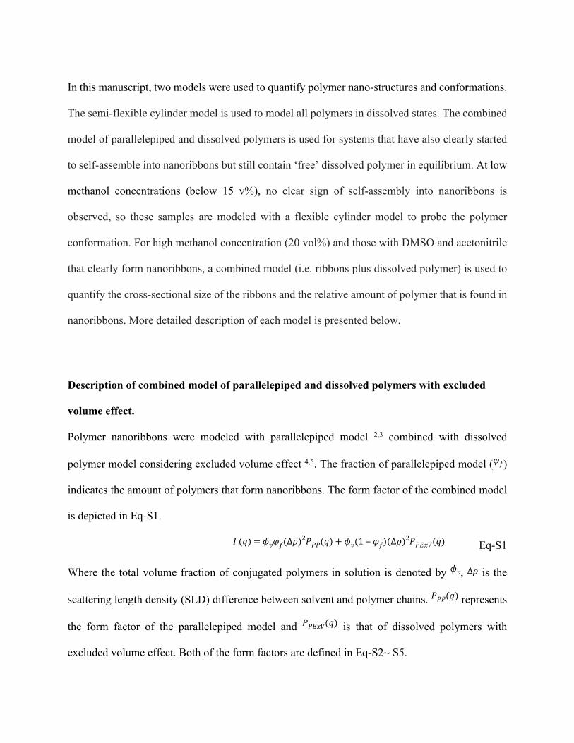
Description of combined model of parallelepiped and dissolved polymers with excluded
volume effect.
Polymer nanoribbons were modeled with parallelepiped model 2,3 combined with dissolved
polymer model considering excluded volume effect 4,5. The fraction of parallelepiped model ( ) 𝜑𝑓
indicates the amount of polymers that form nanoribbons. The form factor of the combined model
is depicted in Eq-S1.
Eq-S1𝐼 (𝑞) = 𝜙𝑣𝜑𝑓(∆𝜌)2𝑃𝑃𝑃(𝑞) + 𝜙𝑣(1 ‒ 𝜑𝑓)(∆𝜌)2𝑃𝑃𝐸𝑥𝑉(𝑞)
Where the total volume fraction of conjugated polymers in solution is denoted by , is the 𝜙𝑣 ∆𝜌
scattering length density (SLD) difference between solvent and polymer chains. represents 𝑃𝑃𝑃(𝑞)
the form factor of the parallelepiped model and is that of dissolved polymers with 𝑃𝑃𝐸𝑥𝑉(𝑞)
excluded volume effect. Both of the form factors are defined in Eq-S2~ S5.

Eq-S2𝑃𝑃𝑃(𝑞) =
2𝜋
2𝜋
∫0
2𝜋
∫0
[(sin (𝑞𝐴sin 𝛼cos 𝛽)𝑞𝐴sin 𝛼cos 𝛽 )(sin (𝑞𝐵sin 𝛼cos 𝛽)
𝑞𝐵sin 𝛼cos 𝛽 )(sin (𝑞𝐶cos 𝛼)𝑞𝐶cos 𝛼 )]2sin 𝛼𝑑𝛼𝑑𝛽
Eq-S3
𝑃𝑃𝐸𝑥𝑉(𝑞) =1
𝑈
12
𝛾( 12
, 𝑈) ‒1
𝑈
1
𝛾(1
, 𝑈)
Eq-S4𝛾(𝑥,𝑈) =
𝑈
∫0
𝑑𝑡 𝑒𝑥𝑝( ‒ 𝑡)𝑡𝑥 ‒ 1
Eq-S5𝑈 =
𝑞2𝑅2𝑔(2 + 1)(2 + 2)
6
Where a and b are the width and height of the parallelepiped, and c denotes the length of the
nanoribbons. As the length of the nanoribbon is over one micrometer, which is outside of the
windown that SANS is probing. The length C of the model is fixed at 1 μm for all the samples.
is the radius of gyration of fully dissolved polymers and ν represents excluded volume paramter, 𝑅𝑔
which is the inverse of Porod exponent.
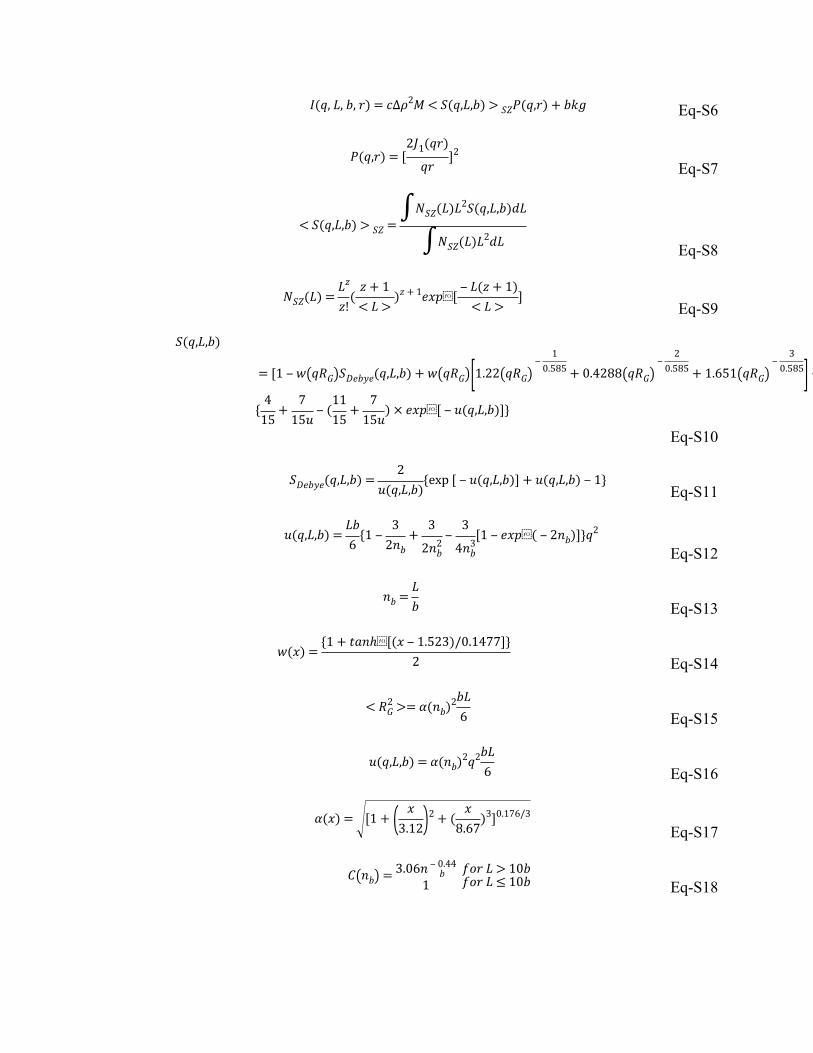
Description of flexible cylinder model with excluded volume effect
For flexible cylinder, each polymer chain is modeled with a contour length of L and a radius of
b. Each polymer chain can be viewed as several rigid rods that are combined. The length of each
rigid rod is called persistent length (lp). Kuhn length (b) is defined as two times of persistent
length, which reflects the rigidity of a polymer chain. The scattering intensity using flexible
cylinder form factor can be modeled with concentration (c), SLD difference ( ), and molecular ∆𝜌
weight (M) as shown in equation S6. 6,7 The scattering functions of single semiflexible chain (
) considering polydispersity of contour length and cross section of a rigid rod ( ) are 𝑆(𝑞,𝐿,𝑏) 𝑃(𝑞,𝑟)
defined from equation S7 to equation S18.
Eq-S6𝐼(𝑞, 𝐿, 𝑏, 𝑟) = 𝑐∆𝜌2𝑀 < 𝑆(𝑞,𝐿,𝑏) > 𝑆𝑍𝑃(𝑞,𝑟) + 𝑏𝑘𝑔
Eq-S7𝑃(𝑞,𝑟) = [
2𝐽1(𝑞𝑟)
𝑞𝑟]2
Eq-S8
< 𝑆(𝑞,𝐿,𝑏) > 𝑆𝑍 =∫𝑁𝑆𝑍(𝐿)𝐿2𝑆(𝑞,𝐿,𝑏)𝑑𝐿
∫𝑁𝑆𝑍(𝐿)𝐿2𝑑𝐿
Eq-S9𝑁𝑆𝑍(𝐿) =
𝐿𝑧
𝑧!(
𝑧 + 1< 𝐿 >
)𝑧 + 1𝑒𝑥𝑝[‒ 𝐿(𝑧 + 1)
< 𝐿 >]
𝑆(𝑞,𝐿,𝑏)
= [1 ‒ 𝑤(𝑞𝑅𝐺)𝑆𝐷𝑒𝑏𝑦𝑒(𝑞,𝐿,𝑏) + 𝑤(𝑞𝑅𝐺)[1.22(𝑞𝑅𝐺)‒
10.585 + 0.4288(𝑞𝑅𝐺)
‒2
0.585 + 1.651(𝑞𝑅𝐺)‒
30.585] +
𝐶(𝑛𝑏)𝑛𝑏
{4
15+
715𝑢
‒ (1115
+7
15𝑢) × 𝑒𝑥𝑝[ ‒ 𝑢(𝑞,𝐿,𝑏)]}
Eq-S10
Eq-S11𝑆𝐷𝑒𝑏𝑦𝑒(𝑞,𝐿,𝑏) =
2𝑢(𝑞,𝐿,𝑏)
{exp [ ‒ 𝑢(𝑞,𝐿,𝑏)] + 𝑢(𝑞,𝐿,𝑏) ‒ 1}
Eq-S12𝑢(𝑞,𝐿,𝑏) =
𝐿𝑏6
{1 ‒3
2𝑛𝑏+
3
2𝑛2𝑏
‒3
4𝑛3𝑏
[1 ‒ 𝑒𝑥𝑝( ‒ 2𝑛𝑏)]}𝑞2
Eq-S13𝑛𝑏 =
𝐿𝑏
Eq-S14𝑤(𝑥) =
{1 + 𝑡𝑎𝑛ℎ[(𝑥 ‒ 1.523)/0.1477]}2
Eq-S15< 𝑅2
𝐺 >= 𝛼(𝑛𝑏)2𝑏𝐿6
Eq-S16𝑢(𝑞,𝐿,𝑏) = 𝛼(𝑛𝑏)2𝑞2𝑏𝐿
6
Eq-S17𝛼(𝑥) = [1 + ( 𝑥
3.12)2 + (𝑥
8.67)3]0.176/3
Eq-S18𝐶(𝑛𝑏) = 3.06𝑛 ‒ 0.44
𝑏1
𝑓𝑜𝑟 𝐿 > 10𝑏𝑓𝑜𝑟 𝐿 ≤ 10𝑏

Figure S8. (a) SANS profiles of DPPDTT with 20 v% and 40 v% n-Hexane. The profiles are fit with flexible cylinder model. (b) The extrapolated contour length, Kuhn Length, and radius from the model.

10-4
10-3
10-2
10-1
100
101
102
I(q)
4 6 80.01
2 4 6 80.1
2 4
q (Å-1)
4 mg/ml PCDTPTin Chloroform mixed withData Fit
0 v% Methanol 10 v% Methanol 15 v% Methanol 20 v% Methanol
Figure S9. 1D SANS scattering profile of 4 mg/ml PCDTPT in chloroform mixed with varied
methanol concentrations. A cylinder model was used to fit the SANS profiles at low methanol
concentrations.
Table S2. Extrapolated fitting parameters for PCDTPT samples from a cylinder model.
Methanol Ratio Radius (nm) Length (nm)
0v% 1.5 30.0
10v% 1.4 39.6
15v% 1.8 38.4

Figure S10. 1-D SANS scattering profiles of d-chloroform mixed with (a) d4-methanol and (b) d14-n-hexane with different ratios.
(1) Xi, Y.; Pozzo, L. D. Electric Field Directed Formation of Aligned Conjugated Polymer
Fibers. Soft Matter 2017, 13, 3894–3908 DOI: 10.1039/C7SM00485K.
(2) Roman Nayuk, K. H. Formfactors of Hollow and Massive Rectangular Parallelepipeds at
Variable Degree of Anisometry. Zeitschrift für Phys. Chemie 2012, 226, 837–854.
(3) P. Mittelbach, G. P. X-Ray Low-Angle Scattering by Dilute Scattering Colloidal Systems.
The Calculation of Scattering Curves of Parallelepipeds. Acta Phys. Austriaca 1961, 14,
185–211.
(4) H. Benoit. La Diffusion de La Lumiere Par Des Macromolecules En Chaines En Solution
Dans Un Bon Solvant. Comptes Rendus 1957, 245, 2244–2247.
(5) Hammouda, B. SANS from Homogeneous Polymer Mixtures - A Unified Overview. Adv.
Polym. Sci. 1993, 106, 87–133.
(6) Pedersen, J. S.; Schurtenberger, P. Scattering Functions of Semiflexible Polymers with
and without Excluded Volume Effects. Macromolecules 1996, 29 (23), 7602–7612 DOI:

10.1021/ma9607630.
(7) Chen, W.-R.; Butler, P. D.; Magid, L. J. Incorporating Intermicellar Interactions in the
Fitting of SANS Data from Cationic Wormlike Micelles. Langmuir 2006, 22 (15), 6539–
6548 DOI: 10.1021/la0530440.