Missing the Marks: Dispersion in Corporate Bond Valuations Across

Mutual Funds*†

Gjergji Cici Assistant Professor of Finance

Mason School of Business College of William & Mary

Williamsburg, VA 23187 USA 757-221-1826 gjergji.cici@mason.wm.edu

Scott Gibson Associate Professor of Finance

Mason School of Business College of William & Mary

Williamsburg, VA 23187 USA 757-221-1673 scott.gibson@mason.wm.edu

John J. Merrick, Jr. Richard S. Reynolds Associate Professor of Business

Mason School of Business College of William & Mary

Williamsburg, VA 23187 USA 757-221-2721 john.merrick@mason.wm.edu

First Draft: November 2007

This Draft: July 15, 2008

*The authors thank Elliot Levine and Andres Vinelli of FINRA; Sean Collins, Brian Reid and Gregory Smith of the Investment Company Institute; and Kenneth Volpert of Vanguard for helpful background discussions. We also thank our discussants and other participants at our presentations at the Financial Industry Regulatory Authority in Washington, DC, the 2008 Financial Management Association European Meetings in Prague, and the 2008 Western Finance Association Meetings in Waikoloa, Hawaii, including Dion Bongaerts, Patrick Herbst, Hsien-hsing Liao and Jeff Pontiff. †This paper received the Society of Quantitative Analysts Award for best paper in quantitative investments at the 2008 Western Finance Association Meetings.

Abstract

We study the dispersion of month-end valuations placed on identical corporate

bonds by different mutual funds. Our dispersion measures offer insights into corporate

bond valuation problems at the individual security level. Results show that pricing

dispersion is related to bond-specific characteristics typically associated with market

liquidity and market-wide volatility. We show that the rollout of FINRA’s transparency-

enhancing TRACE system has increased the precision of corporate bond valuation,

benefiting investors. We also find that the volatile marking patterns of some funds are

associated with return smoothing behavior. However, return smoothing behavior is not

prevalent across our sample of bond mutual funds.

1

How hard is it to mark illiquid securities for position valuation purposes? As it

happens, the issue of accurate marks on the securities positions held by banks, hedge

funds and mutual funds has become a focal point for company boards and regulators and

made front-page news in the financial press during the credit crisis of 2007. Senior

executives of major investment firms have resigned in the midst of significantly revised

write-downs of illiquid structured financial product asset values.1 The SEC is examining

how accurately mutual funds and other investors “value their hard-to-value” securities.2

Furthermore, an investment adviser and several of its employees recently agreed to settle

SEC charges that they negligently mispriced certain bonds owned by two high-yield

municipal bond funds in a way which caused prices for these funds’ shares to be

artificially high.3 Thus, problems regarding the accurate pricing of securities are not

confined to esoteric instruments and have direct implications for both asset allocation and

the integrity of the investment process.4

Our paper analyzes important aspects of US corporate bond pricing and related

issues in bond market structure and transparency by examining the dispersion of month-

end valuations simultaneously placed on identical bonds by an important set of traders:

the managers of US bond mutual funds. A mutual fund’s manager must value the fund’s

bond holdings for net asset value (NAV) purposes. A mutual fund’s net asset value sets

the day’s terms at which fund shares may be purchased and redeemed. A fund should

ensure that its daily NAV is fairly valued. An unfairly valued NAV can result in dilution

of shareholder interests or other harm to shareholders. Thus, funds should strive to price

their individual securities based upon an unbiased and reliable perception of their

respective current values in order to ensure fairness for fund share trading.

1 For example, Stanley O’Neal of Merrill Lynch and Charles Prince of Citigroup each resigned after initial firm estimates of asset write-downs due to the sub-prime credit crisis proved to be substantially understated. 2 As reported in Pulliam, Smith and Siconolfi (2007). 3 See the SEC’s actions versus Heartland Advisors Inc. (http://www.sec.gov/litigation/admin/2008/33-8884.pdf). Heartland’s funds “invested primarily in non-rated, medium and lower quality municipal bonds. The majority of the municipal bonds owned by the Funds were below investment grade and illiquid. Market quotations were not readily available for most of the bonds owned by the Funds. From March 1, 2000 into October 2000, the Funds’ portfolios included several municipal bonds that were valued by the Funds at prices above their fair values. As a result, on numerous days throughout that time period, the Funds’ Net Asset Values (“NAVs”) were incorrect, the Funds’ shares were incorrectly priced, and investors purchased and redeemed Fund shares at prices that benefited redeeming investors at the expense of remaining and new investors.” 4 See Pulliam (2007).

2

But as the credit crisis of 2007 has called into question, the accurate pricing of

individual bond holdings is not always a simple matter. In fact, our study revolves

around examining discrepancies in the price marks that different mutual funds

simultaneously place on identical bond issues. Our data allow us to test how corporate

bond valuation precision may be affected by variables thought to be related to market

liquidity – e.g., issue size and credit rating – as well as any other bond-specific

characteristic such as time to maturity. We also examine the trade reporting initiative

instituted by the Financial Industry Regulatory Authority’s (FINRA) Trade Reporting and

Compliance Engine (TRACE) system for collecting corporate bond trade details from

dealers and disseminating corporate bond transaction price information. We test whether

the increased market transparency due to the staged rollout of TRACE has reduced cross-

fund bond price dispersion in an economically meaningful way.5 Thus, our study has

practical value for a diverse group of stakeholders, including bond trading firms, fund

managers, fund investors and regulators.

Fundamentally, our mutual fund bond valuation data allow us to explore the

difficulty of assessing the current market values of illiquid securities. While illiquid,

corporate bonds are much less opaque than the structured financial products like the

Collateralized Debt Obligations that lay at the heart of the 2007 credit crisis. Thus, our

evidence documenting the difficulties regarding precise assessment of corporate bond

market value is all the more compelling.

Our study makes four contributions. It is the first study to directly measure how

difficult it is to mark positions in the over-the-counter corporate bond market.

Furthermore, our focus on the cross-fund dispersion of a given corporate bond’s

valuation offers direct insight into potential NAV calculation problems at the individual

security level. Related research has previously offered only indirect assessments of the

difficulty of marking securities positions for mutual fund NAV purposes by examining

the staleness of closing prices on exchange-traded equities (see, for example, Chalmers,

Edelen and Kadlec, (2001)) as well as “return smoothing” behavior by hedge funds based

5 The rollout of TRACE began in July 2002 under the auspices of the NASD (National Association of Securities Dealers) to improve corporate bond transparency. FINRA was formed through the consolidation of NASD and the member regulation, enforcement and arbitration functions of the New York Stock Exchange in July 2007.

3

upon serial correlation patterns in security prices and fund returns (see Asness, Krail and

Liew (2001), Bollen and Pool (2006) and Getmansky, Lo and Makarov (2004)). In

contrast, we directly analyze the dispersion of internal marks on identical bonds placed

by mutual funds managers. Second, we find clear evidence that the rollout of TRACE

has decreased cross-fund bond price dispersion even for bonds that were not initially

included in the list of reporting securities. Previous research has found that TRACE has

decreased the trade execution costs of corporate bond trading. Our results here suggest

that the TRACE-induced increase in corporate bond market transparency has benefited

the market more generally by increasing bond valuation precision. Third, we also

uncover and analyze some systematic differences in bond holdings valuations that appear

to incorporate the impact of differences in fund bid versus mid bond value marking

standards. Finally, while we confirm that most funds appear to follow reasonably

consistent pricing policies, our tests also identify certain funds with volatile marking

practices that seem to be associated with return smoothing behavior. This final

investigation adapts a variant of Getmansky, Lo and Makarov’s (2004) framework to

search for serial correlation in fund returns after incorporating a “remarked-at-consensus-

prices” fund portfolio to measure the economic return on any particular fund’s holdings.

Some students of equity markets and equity mutual funds may already be puzzled

with our focus on the dispersion of month-end prices on identical bonds. Unlike equities,

the overwhelming majority of bond trading takes place in over-the-counter dealer

markets instead of on centralized exchanges. Thus, bond mutual funds do not share

common access to a single exchange-determined closing price for each individual bond

issue.6 For some issues, this lack of an exchange-determined closing price is not an

important impediment to valuing a fund’s holding. For example, trading in each of the

most recently auctioned (on-the-run) US Treasury securities is highly liquid and very

transparent. Dealer-to-dealer and dealer-to-customer electronic trading platforms and the

ubiquitous Bloomberg terminal offer continuous pictures of bid and offered prices for

these securities. In stark contrast, most high-yield corporate bond issues trade

infrequently in thin, illiquid markets. Indeed, many individual corporate bond issues are

6 Valuing equities based upon exchange-determined closing prices can also be problematic since such prices for many thinly-traded stocks may be stale. See the fair value discussion below.

4

held mainly as long-term investments in insurance company portfolios and trade very

rarely after an initial distribution period. So it is quite possible that a mutual fund may

need to produce daily NAV valuations for some specific issues that have not traded for

days or even weeks.

We generated our data by merging a comprehensive Morningstar dataset

comprising bond holdings for 2,268 U.S. fixed income mutual funds from January 1995

to December 2006 with the Mergent Fixed Income Securities Database containing

individual bond characteristics such as issue size, credit rating, and maturity. We

supplemented this dataset with data from the TRACE and CRSP Survivor-Bias Free US

Mutual Fund databases. All four databases are free of survivorship bias. Our merged

holdings dataset enables us to identify the price marks reported by all funds holding the

same bond at the same time.

We first examine the cross-fund pricing dispersion of individual bonds. Marking

corporate bonds is hard. Prior to the introduction of TRACE, the interquartile range for

the month-end marks of a typical high-yield bond was about 88 cents (per $100 of par

value). The results show, as expected, that pricing dispersion is related to bond-specific

characteristics typically associated with market liquidity. Specifically, cross-fund pricing

dispersion is lower for higher credit quality bonds; higher for longer maturity bonds; and

lower for larger-sized issues. Our results also show, as expected, that pricing dispersion

for individual bonds increases during periods when interest rate volatility is high.

Our key tests at the individual bond level regarding TRACE examine how the

improved flow of trade reports via TRACE affected the precision of mutual fund bond

pricing. As we later explain, FINRA phased in TRACE over a 27-month period

extending from July 1, 2002 to September 30, 2004. The implementation timetable

differed for bonds in four groups categorized by credit rating and issue size. Bonds in all

four groups experienced economically and statistically significant decreases in cross-fund

pricing dispersion after full implementation of TRACE for their group. For a

representative bond in the group comprising investment grade bonds with an original

issue size greater than $1 billion, the cross-fund interquartile range of pricing marks

5

dropped from 31.9 cents pre-TRACE to 17.3 cents post-TRACE.7 For a representative

bond rated A or higher and issue size between $100 million and $1 billion, the drop was

from 45.9 to 21.8 cents. For a representative bond rated BBB- to BBB+ and issue size

less than $1 billion, the drop was from 59.8 to 22.5 cents. Finally, for a representative

high-yield bond, the drop was from 87.8 to 42.1 cents. Overall, at the individual bond

level, our results show that regardless of credit rating or issue size, pricing marks across

funds became much more precise once TRACE was implemented.

The period over which TRACE was rolled out included a period when some

bonds were included in TRACE while other bonds with similar characteristics were not,

creating a natural experimental setting for our research questions. Consistent with the

pattern above, bonds in TRACE experienced significant decreases in pricing dispersion

across funds. Interestingly, bonds not in TRACE but having similar characteristics

experienced significant decreases in pricing dispersion as well, although of a somewhat

smaller magnitude. This spillover implies that the TRACE reports on trades in eligible

bonds directly helped the market more precisely estimate the current values of related

non-reporting bonds. This result is perfectly reasonable given the “matrix pricing”

approach typically used by bond market professionals to value an illiquid bond on the

basis of any observed prices of other securities with similar coupons, ratings, and

maturities. Furthermore, this result mirrors Bessembinder, Maxwell and Venkataraman’s

(2006) finding that a spillover liquidity effect from the introduction of TRACE resulted

in a trade execution cost reduction even for non-eligible bonds.

Additional empirical tests investigate the tendency for funds to systematically

mark a disproportionate number of individual bond positions in the same direction

relative to the median (consensus) price. We interpret the results as reflecting differences

among funds in the use of mid-market prices versus bid-side prices as the position

marking standard. Even after controlling for differences in fund marking standards, we

continue to find that TRACE increased the precision of mutual fund bond pricing. In

regard to bid versus mid marking standards for NAV purposes, we also show that the

7 Bond prices are quoted as a percentage of face (par) value. We interpret all of our individual bond price data in terms of a $100 face value. Thus, a reported price of 101.50 represents $101.50. Actually, traders would quote this price in the market as 101-16 since the “cents” component is communicated in practice in units of 1/32nds of one percent of par value (the 16 in the 101-16 example quote here refers to 16/32 or .50).

6

choice has economically significant welfare implications for existing, new and redeeming

investors. The welfare implications are particularly significant when a fund experiences

large net inflows or outflows and holds relatively illiquid bonds. This would be true, for

instance, of a small but rapidly growing high-yield corporate bond fund. Intuitively, the

selling of fund shares to new investors at an NAV calculated using bid prices (below

mid-market prices) dilutes existing investors’ claim on the stream of future income

generated by the bond portfolio.

Finally, we investigate whether funds strategically mark bonds to smooth reported

returns. Among the majority of funds that mark bonds consistently at bid or mid prices,

return smoothing does not appear to be prevalent. However, among the minority of funds

that exhibit volatile marking patterns, we find evidence consistent with return smoothing.

Our findings are of importance to bond mutual fund investors. Return smoothing

involves marking positions such that the NAV is set above or below the true value of

fund shares, resulting in wealth transfers across existing, new and redeeming fund

investors. Moreover, return smoothing distorts a fund’s risk-return profile, such as its

Sharpe ratio, perhaps leading investors to make sub-optimal allocation decisions. Our

findings also contribute to the literature on return smoothing by delegated portfolio

managers. To date, researchers have focused on return smoothing behavior by hedge

funds.8 Without direct knowledge of hedge fund holdings, researchers have no choice

but to use hedge funds’ reported returns and rely heavily on econometric techniques to

make indirect inferences about the return smoothing behavior of hedge funds. In

contrast, we directly estimate the true economic return of bond mutual funds’ underlying

assets and thus construct more direct tests of return smoothing behavior.

The remainder of the paper is organized as follows. Section I provides a review

of the related literature. Section II discusses some specific issues related to valuing the

individual holdings of bond funds. Section III discusses our data and summary statistics

on bond fund holdings. Section IV presents our main empirical findings on cross-fund

individual bond price dispersion, fund-by-fund portfolio marking practices and the

impact of TRACE on bond valuation. Section V discusses the impact of bid-price versus

8 See Asness, Krail and Liew (2001), Getmansky, Lo and Makarov (2004) and Bollen and Pool (2006, 2007).

7

mid-price bond marking standards. Section VI investigates the relationship between

marking patterns of certain funds and possible return smoothing behavior. Section VII

concludes.

I. Related literature

Our research touches on themes that have stimulated a number of recent studies in

the academic literature including mutual fund valuation fairness, the relationship between

market transparency and pricing efficiency, and the specific impacts of TRACE on the

US corporate bond market. A key element of concern in the existing literature is the

fairness of current valuations of mutual fund holdings. Two factors undermine the

fairness of the values place on a mutual fund’s holdings: illiquidity of the securities held

and manager discretion over the individual security price marks. Illiquid securities may

be hard to value reliably and may lead to stale fund NAV pricing. For example, the last

observed trade in an illiquid security may have occurred very early in the trading day (or

even on some previous day). Stale prices introduce short-run predictability into a fund’s

returns. A fund that uses last-trade prices to proxy for true end-of-day values on each of

its holdings leaves itself open to market-timing strategies aimed at exploiting stale fund

net asset values. Market-timing traders can exploit such short-run predictability to

expropriate wealth from the fund’s long-term buy-and-hold investors. In addition, an

investment manager may use discretion over individual security marks in order to

manage returns, i.e., alter reported returns to artificially enhance fund performance. This

latter issue goes directly to the heart of the integrity of fund net asset values and fund

returns data and becomes entwined with issues regarding fund manager incentives. Thus,

the most basic questions regard the reliability and fairness of the marks on individual

bond positions set by mutual funds for net asset value (NAV) calculation purposes.

Problems associated with fairly setting daily mutual fund NAVs have been

addressed in the academic literature, especially with regard to the activities of market-

timing traders. As in Chalmers, Edelen and Kadlec (2001), most of the investigations

focus on the impact of nonsynchronous trading effects on fund return predictability.

Equity mutual funds traditionally have used exchange posted last-trade closing prices to

calculate end-of-day NAVs even if the corresponding last trades occurred much earlier in

8

the given trading day. In cases where markets move late in the day, funds using such

stale last-trade prices to calculate end-of-day NAVs become targets for strategic market-

timers. This phenomenon has been shown to be particularly severe for funds that

naturally hold illiquid securities as part of their style – e.g., international equity funds,

small-capitalization equity funds and high-yield corporate bond funds. Bhargava, Bose

and Dubofsky (1998), Boudoukh, Richardson, Subrahmanyam and Whitelaw (2002),

Chalmers, Edelen and Kadlec (2001), Goetzmann, Ivkovic and Rouwenhorst (2001),

Green and Hodges (2002) and Zitzewitz (2003) find evidence of large fund trading flows

and large excess returns to stale price-oriented mutual fund trading strategies. This

research has documented impacts across a large sample of domestic equity, foreign

equity and bond mutual funds. These results have focused attention on the need to

accurately value securities positions for mutual fund NAV calculations. Our focus on the

cross-fund dispersion of mutual fund valuations on a given security offers direct

observations and insights into NAV calculation problems at the individual security level.

The literature has also investigated the relationship between market transparency

and pricing efficiency and, as relates to corporate bonds, the specific impacts of TRACE

on trading costs in the US corporate bond market. This literature distinguishes between

pre-trade transparency (e.g., dissemination of bid and ask quotations, market depth, etc.)

and post-trade transparency (e.g., timely public reporting of price and quantity data from

actual trades). Greater transparency in the trading process may enhance market

performance by reducing the opportunities for professionals to exploit their informational

advantages over less informed or nonprofessional participants (Pagano and Roell (1996)).

Greater transparency may also facilitate improved deterrence and detection of fraud and

manipulation (Edwards, Harris and Piwowar (2007)). However, trade disclosure could

also impede the amount of liquidity made available by dealers to large traders since

disclosure might make it harder for a dealer to unwind large newly-acquired positions

profitably (Biaisa, Glosten and Spatt (2005)).9 Nevertheless, greater transparency is

generally associated with more informative prices (Madhavan (2000)). Indeed,

Bloomfield and O’Hara (1999) assess the impact of trade disclosure on market efficiency

9 For a counter-argument, see Naik, Neuberger and Viswanathan (1999). Gemmil’s (1996) London Stock Exchange evidence suggests that delays in trade reporting do not increase market liquidity.

9

in an experimental setting and find that trade disclosure increases the informational

efficiency of transactions prices.

In this light, the impact of TRACE’s introduction of post-trade price transparency

in the secondary corporate bond market is of particular interest. Indeed, TRACE has

already attracted attention in the market microstructure transactions costs literature.

Bessembinder, Maxwell and Venkataraman (2006) test a simple model of the impact of

transaction reporting on transactions costs. They estimate that TRACE eligibility reduces

trade execution costs by one-half, and that a spillover liquidity effect results in a one-fifth

cost reduction even for non-eligible bonds.10 Edwards, Harris and Piwowar (2007)

estimate average corporate bond transaction costs as a function of trade size. They show

that costs are lower for bonds with transparent trade prices and that such costs drop when

TRACE starts to publicly disseminate bond prices. Goldstein, Hotchkiss and Sirri (2007)

investigate the last-sale trade reporting impact on BBB-rated corporate bond market

liquidity. They find that the effect of post-trade transparency varies with trade size and

has a neutral or positive effect on market liquidity. Except for the case of the most

infrequently traded issues, bid-ask spreads on bonds whose prices become transparent

decline by more than that of a control group.

Bessembinder, Maxwell and Venkataraman’s (2006) framework relates directly to

our study. They analyze the relationship between market transparency and price

efficiency in the context of a world in which transactions costs increase with the variance

of valuation errors.11 They then motivate a presumed salutary impact of the introduction

of TRACE on transactions costs by focusing on the role of improved precision in

estimating corporate bond value. Here, we directly study shifts in bond valuation

precision associated with the rollout of TRACE via our analysis of cross-fund dispersion

of mutual fund valuations. This offers a lens through which to directly view the impact

of TRACE on bond valuation precision. Moreover, in contrast to previous studies, our

data span the entire time period of the four-phase roll-out of the TRACE system. We test

10 This finding is consistent with a related liquidity externality found for Tel Aviv Stock Exchange securities by Amihud, Mendelson and Lauterbach (1997) since improved price discovery for one security improves price discovery for other related securities. 11 Bessembinder, Maxwell and Venkataraman (2006) offer two channels for such a relationship: greater valuation errors (1) may increase the inventory risks of market-making and (2) may increase the likelihood that dealers can extract rents from less-well-informed counterparties.

10

for the marginal impacts that increased post-trade price transparency has had on the

precision of individual corporate bond value assessment. In particular, we track whether

increased post-trade transparency during the TRACE roll-out led to more precise value

assessment as indicated by associated decreases in the cross-fund dispersion of mutual

fund marks on individual bonds.

II. Pricing bond holdings for mutual fund NAV purposes

A fund’s net asset value sets the day’s terms at which fund shares may be

purchased and redeemed. A mutual fund should ensure that its daily NAV is fairly

valued. If a fund’s NAV is overstated, redeeming shareholders will receive a windfall

that comes at the expense both of other shareholders who remain in the fund and new

purchasing shareholders who pay too much for the shares. Likewise, if a fund’s NAV is

understated, redeeming shareholders will lose out both relative to other shareholders who

remain in the fund and new purchasing shareholders who pay too little to acquire their

shares. Thus, proper pricing of fund portfolio securities is necessary to ensure fairness

among all fund shareholders. As previously discussed, trading strategies exploiting

return predictability due to biases in NAVs have generated large excess returns.

Under the Investment Company Act of 1940, the definition of “value” is

construed in one of two ways. Securities for which “readily available” market quotations

exist must be valued at market value. All other securities must be priced at “fair value”

as determined in good faith according to processes approved by the fund’s board of

directors. Marking a particular security at a fair value requires a determination of what

an arm's-length buyer, under the circumstances, would currently pay for that security.

A. Marking positions using readily available market quotations

As stated in an April 2001 SEC Division of Investment Management letter to the

Investment Company Institute, “funds must exercise reasonable diligence to obtain

market quotations for their portfolio securities before they may properly conclude that

market quotations are not readily available. If, for example, a fund obtains market

quotations for a portfolio security from one source and determines that they are

unreliable, the fund should diligently seek to obtain market quotations from other

11

sources, such as other dealers or other pricing services, before concluding that market

quotations are not readily available.”12 Thus, funds are not permitted to ignore these

readily available quotations and mark a given position at an internally-generated fair

value price. However, for example, a foreign equity fund using stale last-trade closing

prices to mark positions is responsible for monitoring for significant events (including

general market volatility) that would cause local closing prices to not be considered

reliable readily available market prices (Zitzewitz, 2003).

Bond dealer firms and securities pricing services compile daily marks on

individual issues. Dealers compile these marks for internal profit and loss determination,

repurchase agreement transaction collateral valuation, bond index construction and client

servicing purposes. Within each dealer firm, the marks on a given security are generally

set by the trading desk responsible for dealing in that security. Traders use available

quotes from inter-dealer broker screens on the subject security or related securities, their

own customer flows and any available “market color” – stories behind the day’s

transactions relayed from a variety of sources – as inputs to the marking process.

Furthermore, compliance and risk management professionals within the dealer firm

typically review the appropriateness of these marks, especially with regard to the

integrity of internal daily profit and loss figures.13 Dealers provide a great deal of

information concerning prices, relative value and insights to institutional buy-side

customers. Generally, there is effective best-in-class price knowledge for buy-side

customers that have multiple (e.g., five) dealer relationships and access to price quotes

from dealer sources.14

Securities pricing services produce and offer marks derived from analysis of

various sources. Pricing services are for-profit firms that provide prices and pricing-

related data to financial institutions like mutual funds for a fee. Pricing services compete

for business along dimensions of pricing quality, security coverage and data transmission

reliability.15 These data cover both listed market price data for exchange-traded

12 http://www.sec.gov/divisions/investment/guidance/tyle043001.htm 13 See Pulliam (2007). 14 See “An analysis and description of pricing and information sources in the securitized and structured finance markets,” The Bond Market Association and The American Securitization Forum, October 2006. 15 Two of the more important pricing services for evaluated pricing are FT Interactive Data and Standard & Poor's Security Evaluation Services. Others are Reuters Enterprise Information, Bear Stearns PricingDirect

12

securities and “evaluated” price data for over-the-counter market securities. The price

data for the exchange-listed securities are collected from the exchanges. An “evaluated”

price for an over-the-counter market security is produced from firm-specific

methodologies that combine information from a number of sources as well as

professional judgment. A price needs to be produced each day even if the security in

question did not trade that same day. Over-the-counter debt market securities such as US

Treasury securities are easy to price. The US Treasury market has transparent, liquid

markets for a set of benchmark on-the-run issues. The easily observable quotes on these

benchmark issues can be used to value other less liquid, off-the-run issues via standard

techniques. However, other over-the-counter debt market securities such as high-yield

corporate bonds and distressed debt are more difficult to value. The precision by which

such securities can be mechanically marked off of liquid securities like Treasuries or

liquid derivatives like Libor-based interest rate swaps is low. Instead, such securities

need to be “hand-priced” using an information set that may include actual transaction

prices reported during the day by TRACE, indicative bids or offers obtained from bond

dealers, and concurrent prices of related securities or derivative contracts.

Thus, as a practical matter, a mutual fund could comply with the Investment

Company Act’s mandate to mark bond positions using “readily available” market

quotations by relying on a single pricing service or multiple securities pricing services

and/or securities dealers for the fund’s holdings. The fund could adhere to mechanical

rules to use a predetermined single source or combine information from a number of

sources, or else sometimes utilize discretion in adjustments to the individual security

marks. Some funds outsource the actual fund accounting function to firms specializing in

that function, while other funds, especially those organized within a large family of

funds, perform the fund accounting function in-house.

and Telekurs Financial. Some providers like derivatives specialist Markit Group and Canadian debt specialists SVC Corp. and FRI Corp. focus on specific asset classes. See the March 23, 2007 industry overview article published in Advanced Trading: http://www.advancedtrading.com/showArticle.jhtml;jsessionid=T0ABWVMTEFC1YQSNDLRCKH0CJUNN2JVN?articleID=198500315. For a listing of industry pricing sources relevant for securitized and structured financial products, see “An analysis and description of pricing and information sources in the securitized and structured finance markets,” The Bond Market Association and The American Securitization Forum, 2006.

13

B. Marking positions using fair value

Even an exchange-listed security’s price may sometimes be supplanted by an

evaluated price. Such a listed security’s evaluated price is also called a “fair value” price.

The intent of fair value pricing is to protect long-term fund investors from strategic short-

term investors who seek to take advantage of funds as a result of significant events

occurring after the underlying securities last trade, but before the fund’s NAV

calculation. SEC Accounting Series Release Nos. 113 and 118 recognize that no single

standard exists for determining fair value. By the SEC’s interpretation, a board acts in

good faith when its fair value determination is the result of a sincere and honest

assessment of the amount that the fund might reasonably expect to receive for a security

upon its current sale, based upon all of the appropriate factors that are available to the

fund. Fund directors must "satisfy themselves that all appropriate factors relevant to the

value of securities for which market quotations are not readily available have been

considered and to determine the method of arriving at the fair value of each such

security."16 Interestingly, under the SEC’s interpretation, different fund boards, or funds

in the same complex with different boards, could reasonably arrive at prices that were not

the same when fair value pricing identical securities.

As it happens, the over-the-counter dealer market arrangement of bond markets

and general reliance on dealer and/or pricing service marks for individual securities make

bond funds generally less susceptible to stale pricing problems that are related to overall

market volatility. In particular, bond dealers and bond pricing services will mark

individual securities by “matrix pricing” on an option-adjusted yield spread (“OAS”)

basis against the heavily-traded US Treasury benchmark issues. In this manner, the

entire set of bond universe marks will reflect the latest available general market moves

through Treasury benchmarks. But because so many corporate bond issues are illiquid

and infrequently traded, there tends to be substantial variation in valuations nonetheless.

For example, different dealers will experience different customer flows and therefore

16 Subsequent SEC guidance has outlined four obligations for mutual funds relating to fair valuation: (1) adopt written policies and procedures that require the fund to monitor for circumstances that may necessitate the use of fair value pricing; (2) establish criteria for determining when market quotations are not reliable for a particular security; (3) establish methodologies to determine the current fair value of a security; and (4) regularly review the appropriateness and accuracy of the security valuation methods. See “An introduction to fair valuation,” Investment Company Institute, ICI Mutual Insurance Company and the Independent Directors Council, 2005.

14

may form different opinions about the underlying value of any infrequently traded issue.

The information a bond dealer collects through seeing specific customer trading flow

goes beyond the trade’s price. The size of the trade, the identity of the customer, and any

explanations from the customer about the reasons behind the trade all matter. Thus, a

dealer who has not traded a particular illiquid bond for an extended period will have a

less informative opinion on its current value than one who has recently traded it.

Zitzewitz (2003) finds some evidence of NAV predictability in high-yield bond funds.

Such evidence is at least partially consistent with the view that some price staleness may

still be a problem for bond funds. Nevertheless, grossly inefficient extrapolative

valuation rules should not survive competitive pressures within the pricing services

industry. Indeed, such pricing services should seek to distinguish themselves by doing a

good job of hand-pricing infrequently traded “hard-to-mark” securities. Thus, given the

incentives in place, we would expect that pricing services would generate unbiased

valuations of even the hardest-to-mark securities.

Variation among the valuations used by different mutual funds for the same

corporate bond can be attributed to a number of factors. Some of these factors relate to

the underlying valuation analytics. Important differences may exist in the specific inputs

and models used by price providers to develop the pricing matrix applicable to the

individual corporate bonds. Price services seek to differentiate themselves in the eyes of

subscribing funds through offering “best-in-class” methodologies. But other factors

driving variation in bond valuations will relate to choices made by the funds themselves.

Specifically, pricing services may provide a menu of marking alternatives that permit any

subscribing fund to choose either 3:00 PM or 4:00 PM benchmark Treasury yield curves

as the “closing” benchmark curve. Furthermore, some pricing services offer funds the

choice of marking the positions either at “bid” prices or at “mid” prices.17 We will

provide some insights into the theoretical and empirical importance of this “bid” versus

“mid” choice in later sections of this paper.

III. Data and mutual fund corporate bond ownership statistics

17 The pricing service would develop an estimate of the “bid-ask” spread for each bond and then subtract half of this spread from the bond’s mid price to produce a “bid” price.

15

A. Data

We use four databases in our study: (1) the Morningstar mutual fund holdings

database, (2) the CRSP Survivor-Bias Free US Mutual Fund Database, (3) the Mergent

Fixed Income Securities Database (FISD), and (4) the TRACE (Trade Reporting and

Compliance Engine) database, which reports over-the-counter (OTC) corporate bond

trades.

From Morningstar, we obtained mutual fund holdings data from January 1995 to

December 2006 for 2,268 funds classified as fixed income funds. For each fund and date,

the Morningstar mutual fund holdings database reports the CUSIP identifier of each

security held and both the market and face values of each particular security holding.

Based on the available Morningstar investment categories, each fund falls into one of

four broad groups: Corporate Bond Funds, Government Bond Funds, Municipal Bond

Funds, and Foreign Bond Funds. The database includes both surviving and dead funds

and reports many additional statistics for each period in which a fund had a holdings

report. Some of these fund statistics include an average maturity score, average credit

quality, average duration, and several additional portfolio composition variables such as

percentage invested in: government bonds, corporate bonds, bonds of a particular credit

rating (e.g., AAA or BBB), etc. Although funds were mandated to publicly report

holdings only semiannually until 2004 and quarterly thereafter, some funds voluntarily

reported holdings to Morningstar monthly.

From the CRSP Survivor-Bias Free Mutual Fund Database, we obtained monthly

mutual fund returns. The Morningstar and CRSP databases were merged using

algorithms based on matching fund tickers and fund names. Over the 2003-2006 period

when both databases reported bond holdings, our matching algorithm was supplemented

with matches for holding positions. Out of the 2,268 funds in Morningstar we were able

to find a match for 2,123 funds from the CRSP Database.18

From FISD, we obtain the credit rating, coupon rate, maturity date and issue size

for a given bond at a particular point in time. We merged FISD with Morningstar

holdings using bond CUSIPs.

18 CRSP mutual fund return data is reported at the fund share class level and not at the portfolio level. We computed a single portfolio return each month by averaging the returns of all share classes belonging to a common portfolio after weighting the returns of each share class by the assets of each share class.

16

Finally, from the TRACE database, we identified for each bond the time interval

over which trade reports appeared in the database. We merged the TRACE data with the

rest of the data using bond CUSIPs. As we later describe, to identify TRACE-eligible

bonds during the transition period, we check whether each bond each month appeared in

the TRACE database. During the transition phase, we presume that a bond was TRACE

eligible over the period extending from the first to last appearance of a trade report in the

TRACE database.

B. Mutual fund ownership profiles of corporate bonds

We use two measures to quantify and assess bond mutual fund ownership

characteristics for different types of bonds. This first measure, Own Ratio, is calculated

for each bond in a given year as the percentage of the issue size held by all 2,268 bond

mutual funds. The second measure, Own Number, is calculated for each bond in a given

year as the number of funds holding that bond. As in Falkenstein (1996), both of these

measures are calculated every year and use the latest holdings report in a given year for a

given mutual fund. The average and median values reported in Table I are taken across

year-bond observations. There are 71,758 year-bond observations corresponding to a set

of 15,291 non-convertible corporate bond securities categorized as such by FISD.

<Insert Table I about here>

Panel A of Table I reports ownership statistics for all bonds. Panel B reports

mean and median values for the ownership statistics by credit rating group. Each credit

rating group suppresses the half-step distinctions (e.g., AAA-, AAA, and AAA+ bonds

are all categorized as AAA). Panel C reports statistics categorized by the size of the

issue. Each year, bonds are ranked on issue size and placed into deciles where the

highest-issue-size bonds are placed in Decile 1 and lowest-issue-size bonds are placed in

Decile 10. Ownership statistics categorized into 4 groups defined by the time to maturity

are reported in Panel D.

The results in Table I reveal that the ownership impact of bond mutual funds on

the corporate bond market tends to be relatively more concentrated in the intermediate

17

maturity and high-yield sectors. For example, the median Own Ratio for high-yield

bonds is more than four times the corresponding value for investment grade bonds.

Perhaps more striking, the median Own Ratio for B-rated bonds is almost ten times the

corresponding value for AAA-rated bonds. Across the maturity spectrum, mutual funds

own substantially higher fractions of outstanding issues in the intermediate 5-to-10-year

sector than they do in other maturity sectors. For example, the median Own Ratio for 5-

to-10-year issues (7.67%) is more than double the corresponding value for the >10-year

issues (3.59%). There does not appear to be any issue size-related tendency regarding

mutual fund participation as measured by the Own Ratio. However, the results for Own

Number measure clearly reveal that the largest issues are the most widely-held. In the

issue-size dimension, the median number of funds holding a top-decile bond is 21, while

the median number of funds holding a bottom-decile bond is just 1. The Own Number

results for our sample of mutual funds suggest that large-sized, 5-to-10-year maturity,

high-yield bonds are the most widely-held corporate issues.

IV. Cross-fund price dispersion for the overall sample of funds

A. Measures of bond price dispersion

For each fixed income fund and each reporting period, the Morningstar mutual

fund holdings database reports the market value of each bond holding together with the

face value of the position. To calculate the reported price of bond i held by fund j at date

t, i,j,ticePrportedRe , we divide the reported market value of that bond holding by the

reported face value of the holding and then multiply by 100. In other words, the reported

price measure that we use can be interpreted as the price per each 100 dollars of face

value. For a bond to be included in our sample, three or more funds must report the price

of the identical bond as of the same date.19 Our sample includes 11,116 distinct corporate

bonds and 252,765 bond-date observations that satisfy this condition.

To measure bond price dispersion across funds, we compute the interquartile

range (IR), standard deviation (STD), and average median absolute deviation (MAD) of

19 We also ignored all bond positions that were smaller than $10,000 in par value and round the ratio of the reported market value to the reported face value of the holding to the fourth decimal point to avoid spurious differences due to rounding errors.

18

prices reported by all the funds holding the same bond on the same date. We use the

interquartile range and the average median absolute deviation in addition to the standard

deviation because the distribution of bond prices across funds is negatively skewed and

normality is rejected by the Smirnov-Kolmogorov and Anderson-Darling tests at the 1

percent and 0.5 percent level, respectively.20 The resulting dispersion statistics are then

averaged across bond-date observations.

B. Univariate sorts

Table II reports bond price dispersion statistics based on univariate sorts related to

bond characteristics. Panel A reports dispersion statistics by credit rating group. As

expected, pricing dispersion across funds is generally decreasing in bond credit quality.

Panel B reports dispersion statistics by the size of the issue. Bonds are ranked on issue

size annually and then placed into deciles. The highest-issue-size bonds are placed in

Decile 1 and the lowest-issue-size bonds are placed in Decile 10. Also as expected,

dispersion is nearly monotonically decreasing in issue size. Panel C reports dispersion

statistics categorized into four groups defined by the time to maturity. Again as expected,

dispersion is increasing in time-to-maturity.

<Insert Table II about here>

C. Multivariate regressions

We next relate bond price dispersion to bond characteristics in a multivariate

setting via pooled regressions of bond price dispersion measures on two sets of

independent variables. The dependent variable in each regression is a dispersion measure

alternatively quantified as the interquartile range (IR), standard deviation (STD), and

average median absolute deviation (MAD) of prices reported by all the funds holding the

same bond on the same date. The first set of independent variables include the following

bond characteristics: Issue Size (log of the original face value of a bond issue expressed

in millions of dollars); Maturity (log of the remaining time to maturity of the bond

20 The fact the Anderson-Darling test rejects normality at an even lower significance level is consistent with the fact that this test puts more weight on the tails than the Smirnov-Kolmogorov and that the bond price data is negatively skewed.

19

expressed in years); Rating Code (a discrete variable ranging from 1 for AAA rated

bonds to 22 for D rated bonds). The second set of independent variables include:

Volatility, which is the annualized standard deviation of daily percentage price changes

for the 10-year Treasury Note Futures during the concurrent observation month; TRACE

Transition Dummy, which takes the value one for observations between July 1, 2002 and

September 30, 2004 (when TRACE was partially implemented) and zero otherwise; and

Full TRACE Dummy, which takes the value one for observations after September 30,

2004 (when TRACE was fully implemented) and zero otherwise.

Table III presents results for the multivariate analysis of bond price dispersion.

The computed t-statistics are based on Rogers (1993) standard errors clustered by bond.

As for the univariate analysis, results show that pricing dispersion is related to bond-

specific characteristics typically associated with market liquidity and value uncertainty.

Again, cross-fund pricing dispersion is decreasing in a bond’s credit quality, increasing in

its time-to-maturity, and decreasing in its issue size. Results also show, as expected, that

pricing dispersion for individual bonds increases during periods when interest rate

volatility is high. The key results in Table III are the loadings on the TRACE Transition

Dummy and the Full TRACE Dummy. The negative and significant loadings are

consistent with the improved flow of trade reports via TRACE increasing the precision of

mutual fund bond pricing. The decline in dispersion across funds appears economically

significant as well. When we restrict the impact relative to the pre-July 1, 2002 period to

be the same for all bonds (as the specifications in Table III do), the interquartile range

narrowed by 29.5 cents during the TRACE transition period and 36.0 cents once TRACE

was fully implemented.

<Insert Table III about here>

Our next set of multivariate regressions allow for differing TRACE effects for

four groups categorized by credit rating and issue size. The groups correspond to bond-

characteristic criteria specified by FINRA in its phased implementation of TRACE over

the 27-month period extending from July 1, 2002 to September 30, 2004. The first group

of bonds, or Set I bonds, comprises all investment grade bonds greater than $1 billion in

20

original issue size. Bonds meeting these specifications became permanently TRACE-

eligible as of July 1, 2002. For Set I bonds, we run the same pooled multivariate

regression as in Table III, but with the following changes to the model specification: The

Credit Rating and Issue Size variables are excluded given Set I bond’s homogeneity

along these dimensions, and the Full TRACE Dummy takes a value of one for

observations after July 1, 2002 and zero otherwise. The second group of bonds, or Set II

bonds, includes all investment grade bonds rated A or higher with original issue size of

$100 million or higher. Bonds meeting the Set II specifications became permanently

TRACE-eligible as of March 1, 2003. For Set II bonds, we modify the regression model

specification in the same way, but with the Full TRACE Dummy taking a value of one for

observations after March 1, 2003 and zero otherwise. The third group of bonds, Set III

comprises all bonds rated BBB- to BBB+ with an original issue size less than $1 billion.

On March 31, 2003 FINRA required the reporting of transaction information for 90

bonds meeting these criteria and on April 14, 2003 expanded the list to 120 bonds. All

bonds meeting the criteria became permanently TRACE-eligible as of October 1, 2004.

While the number of TRACE-eligible bonds meeting the criteria was first constant at 90

bonds and later constant at 120, the composition changed. To identify TRACE-eligible

bonds over the transition period, we check whether each bond each month appeared in

the TRACE database. During the transition phase, we presume that a bond was TRACE

eligible over the period extending from the first to last appearance of a trade report in the

TRACE database. For all bond-month observations falling on this TRACE-reporting

timeline, we code the TRACE Eligible Dummy equal to one and zero otherwise. For

bond-month observations not falling on the TRACE-reporting timeline, we code the

TRACE Ineligible Dummy equal to one and zero otherwise. The Full TRACE Dummy

takes a value of one after September 30, 2004 and zero otherwise. Finally, the fourth

group of bonds, Set IV, includes all high yield bonds. On July 1, 2002 FINRA required

the reporting of transaction information for 50 high yield bonds. All high yield bonds

became permanently TRACE-eligible as of October 1, 2004. The number of TRACE-

eligible high yield bonds stayed constant at 50 over the transition period but the

composition changed. For high yield bonds, we construct a TRACE Eligible Dummy,

21

TRACE Ineligible Dummy, and Full TRACE Dummy in a manner analogous to that

described above.

Table IV reveals that bonds in all four groups experienced economically and

statistically significant decreases in cross-fund pricing dispersion after full

implementation of TRACE for their group. To get a sense of the economic magnitude of

the decrease in pricing dispersion, we interact the Maturity and Volatility loadings with

their approximate median values of 5 years-to-maturity and 6 percent per year,

respectively. For a representative Set I bond (i.e., investment grade bonds with an

original issue size greater than $1 billion), the cross-fund interquartile range of pricing

marks dropped from 31.9 cents before TRACE to 17.3 cents after full implementation of

TRACE. For a representative Set II bond (i.e., A or higher rated bonds with an issue size

between $100 million and $1 billion), the drop was from 45.9 to 21.8 cents. For a

representative Set III bond (i.e., BBB- to BBB+ rated bonds with an issue size less than

$1 billion), the drop was from 59.8 to 22.5 cents. Finally, for a representative Set IV

bond (i.e., high-yield bonds), the drop was from 87.8 to 42.1 cents. Overall, our results at

the individual bond level show that regardless of credit rating or issue size, cross-fund

price dispersion decreased after TRACE was implemented.

<Insert Table IV about here>

As we described above, FINRA’s phased approach to the implementation of

TRACE included a period when some bonds rated BBB- to BBB+ with issue sizes less

than $1 billion and high yield bonds were TRACE-eligible while other bonds with similar

characteristics were not, creating a natural experimental setting for our research

questions. The loading on the TRACE Eligible Dummy in Panel B of Table IV is

consistent with TRACE-eligible bonds experiencing significant decreases in pricing

dispersion across funds. Interestingly, the loadings on the TRACE Ineligible Dummy are

consistent with non-eligible, but otherwise similar, bonds experiencing significant

decreases in pricing dispersion as well, although of a somewhat smaller magnitude. This

spillover implies that the TRACE reports on trades in eligible bonds directly helped the

market more precisely estimate the current values of related non-reporting bonds. This

22

result is reasonable given the matrix pricing approach typically used by bond market

professionals to value an illiquid bond on the basis of any observed prices of other

securities with similar coupons, ratings, and maturities. Furthermore, this result mirrors

Bessembinder, Maxwell and Venkataraman’s (2006) finding that a spillover liquidity

effect from the introduction of TRACE resulted in trade execution cost reductions even

for non-eligible bonds.

V. “Mid” versus “bid” bond pricing

A. Institutional details

SEC Accounting Series Release No. 118 provides guidance on how investment

companies should value over-the-counter securities like corporate bonds to be in

compliance with the Investment Act of 1940:

“Because of the availability of multiple sources, a company frequently has a

greater number of options open to it in valuing securities traded in the over-the-

counter market than it does in valuing listed securities. A company may adopt a

policy of using a mean of the bid prices, or of the bid and asked prices, or of the

prices of a representative selection of broker-dealers quoting on a particular

security; or it may use a valuation within the range of bid and asked prices

considered best to represent value in the circumstances. Any of these policies is

acceptable if consistently applied. Normally, the use of asked prices alone is not

acceptable.”

The SEC’s guidance suggests that mutual funds should either be choosing to mark

bond values at the bid price or at the mid-market price (i.e., the average of the bid and ask

prices). The choice between employing a bid or mid valuation concept is important for

markets like high-yield corporate bonds where bid-ask spreads can be relatively wide.

Regarding mutual fund accounting issues, FASB 157 on Fair Value Measurements issued

in September 2006 also specifies that the price within the bid-ask spread that is most

representative in the circumstance should be used to measure fair value.

We checked these pricing guidelines against how mutual funds report their debt

securities pricing practices by examining Prospectuses together with the Statements of

Additional Information of several bond funds. Consistent with the SEC’s guidance, we

observed that some funds explicitly described a practice of marking their debt securities

23

using bid marks,21 whereas some other funds described a practice of marking debt

securities using mid marks.22 Alternatively, some other funds did not provide much

detail about their pricing practice beyond mention of using pricing services as price

sources.

B. Categorizing funds by pricing standard

We investigate the bid and mid pricing practices of our sample funds by exploring

the tendency for funds to systematically mark a disproportionate number of individual

bond positions in the same direction relative to the consensus (i.e., the cross-sectional

sample median) price. If the underlying process driving the dispersion in individual

position marks is random, and if all funds mark their bond positions using a common

standard (i.e., mid pricing or bid pricing), then the number of positions marked above the

consensus price for a particular fund on a particular date should roughly equal the number

marked below. We screen for funds that mark a disproportionately large fraction of

individual bond positions above consensus prices. We also screen for funds that mark a

disproportionately large fraction of individual bond positions below consensus prices.

We use this screening process to infer the pricing standard used by the fund to mark

bonds for NAV purposes. Intuitively, our process presumes that a fund observed

marking the vast majority of its bonds below consensus prices on a given date is marking

bonds at bid prices, whereas a fund observed marking the vast majority of its bonds

above consensus prices on a given date is marking bonds at mid prices.

We follow a three step process that places each fund in a given sample period into

one of six pricing categories: presumed mid marker, presumed bid marker, unclassifiable

marker, bid-to-mid switcher, mid-to-bid switcher, or volatile marker. First, for each fund

report date, we determine whether the mark of each bond held was above, equal to, or

21 The following is an example of language used in the prospectus of a fund that uses a bid marking pricing standard: “Securities that are not traded primarily on an exchange generally are valued

using latest quoted bid prices obtained by an independent pricing service” (see http://www.sec.gov/Archives/edgar/data/1081400/000119312508071373/0001193125-08-071373.txt). 22 The following is an example of a fund that uses a mid mark pricing standard: “Securities for which

market prices are not provided by any of the above methods may be valued based upon quotes furnished by

independent sources and are valued at …in the case of debt obligations, the mean between the last bid and

ask prices” (see http://www.sec.gov/Archives/edgar/data/842790/000095012908002505/0000950129-08-002505.txt).

24

below the consensus price. Second, each fund date is screened for systematically high

marks using a binomial test based on the number of bonds marked above consensus

prices relative to the total number of bonds.23 To ensure that our inferences are based on

sufficient data, our sample only includes dates when funds report holdings for ten or

more bonds with valid consensus prices. This restriction produces a sample of 930

funds.24 Fund dates are recorded as “up dates” when the majority of individual positions

have marks above consensus prices such that the one-sided p-value from the binomial test

is less than five percent under the null that marking individual positions above or below

the consensus price is equally likely. Fund dates are recorded as “down dates” in an

analogous fashion. Thus, each date for which a fund reports portfolio holdings is

categorized as an “up date,” a “down date” or remains an “unclassified date.” In the third

step, a fund is categorized as a presumed mid marker if no date for that fund can be

categorized as a “down date” and the rest of the dates are categorized as a mixture of “up

dates” and “unclassified dates.” A fund is categorized as a presumed bid marker if no

date for that fund can be categorized as an “up date” and the rest of the dates are

categorized as a mixture of “down dates” and “unclassified dates.” A fund is categorized

as an unclassifiable marker if all its portfolio dates are “unclassified dates.” A fund is

categorized as a bid-to-mid switcher if the classification of its portfolio dates changed

once from “down dates” to “up dates.” A fund is categorized as a mid-to-bid switcher in

a similar way. Finally, a volatile marker is a fund that experienced multiple changes in

the classification of its portfolio holdings report dates from “down dates” to “up dates” to

“down dates” again, or vice versa. As a robustness check, we repeat the above

classification process using only the fund’s 20 bonds with the lowest expected price

dispersion.25

23 We include position marks equal to the consensus price in the total number of bonds to reduce the probability of making Type I errors for up and down date calculations. 24 Although the restricted sample of 930 funds includes some funds not explicitly classified as corporate bond funds such as government bond funds with substantial investments in corporate bonds, 92% of the funds are corporate bond funds. 25 This is an attempt to increase the signal to noise ratio of our categorization algorithm. Expected price dispersion for a given bond is calculated from a pooled regression where the dependent variable is bond price dispersion measured as the interquartile range (IR) of prices reported by all funds holding the same bond on the same date and the independent variables are: Issue Size (log of the original face value of a bond issue expressed in millions of dollars); Maturity (log of the remaining time to maturity of the bond expressed in years); Rating Code (a discrete variable ranging from 1 for AAA rated bonds to 22 for D rated

25

Panel A of Table V reports the frequency of funds in each of the six pricing

standard categories for the overall sample period (01/31/1995-12/31/2006), the pre-

TRACE period (01/31/1995-06/30/2002), and the post-TRACE period (10/31/2004-

12/31/2006). In Panel A.1, the categorization algorithm uses all of the bonds held by the

fund. In Panel A.2, the categorization algorithm uses only the 20 bonds with the lowest

expected price dispersion from among those held by each fund. Panel A.1 shows that

presumed mid markers and presumed bid markers together comprised about two-thirds of

the overall and pre-TRACE period samples and more than three-quarters in the post-

TRACE period sample. Specifically, presumed mid markers comprised 27.5%, 29.0%,

and 34.8% of the sample in the overall, pre-TRACE, and post-TRACE periods,

respectively.26 Presumed bid markers comprised slightly higher percentages during these

periods at 36.0%, 38.1%, and 42.1%, respectively. Interestingly, the third largest

category in the overall period was volatile markers at 16.77%. The volatile markers

exhibited a pattern consistent with switching their marking standard at least twice. For

example, a volatile marker might first have marked a disproportionate number of bonds

above consensus prices, then below, and then above again. Or else a volatile marker

might first have marked a disproportionate number of bonds below consensus prices, then

above, and then below again. Even over the shorter pre-TRACE and post-TRACE

subperiods, volatile markers comprised 6.7% and 5.1% of the samples, respectively.

Panel A.2 shows that results are similar when only bonds with low expected pricing

dispersion are used to categorize funds.

<Insert Table V about here>

Panel B of Table V reports the frequency of funds in each category during the

post-TRACE period contingent upon their categorization during the pre-TRACE period.

Funds that were no longer in existence post-TRACE or that had insufficient data post-

bonds); and Volatility, which is the annualized standard deviation of daily percentage price changes for the 10-year Treasury Note Futures. 26 The frequency of presumed mid markers in the pre-TRACE period is reasonably similar to the estimate reported in the Capital Market Risk Advisors’ survey conducted in 2000 and summarized by Rahl (2001). In that survey, 38% percent of the mutual fund respondents (which included both bond and equity funds) indicated that they used a mid-market pricing standard.

26

TRACE are categorized as dead funds. Again Panel B.1 uses all of the fund’s bonds to

categorize funds and Panel B.2 uses only the fund’s 20 bonds with the lowest expected

price dispersion. Panel B.1 shows that a majority of presumed mid markers in the pre-

TRACE period continued to be categorized as presumed mid markers in the post-TRACE

period. Of the 205 presumed mid markers in the pre-TRACE period, 118 (or 57.6%)

were categorized as presumed mid markers in the post-TRACE period. When the 40

dead funds in the post-TRACE period are excluded, the 118 presumed mid markers in the

post-TRACE period represent 71.5% of the remaining 165 presumed mid markers in the

pre-TRACE period. Presumed bid markers exhibit similar stability across the pre- and

post-TRACE subperiods. Of the 269 presumed bid markers in the pre-TRACE period,

150 (or 55.8%) were categorized as presumed bid markers in the post-TRACE period.

When the 50 dead funds are excluded, the 150 presumed bid markers in the post-TRACE

period represent 68.5% of the remaining 219 presumed bid markers in the pre-TRACE

period. We also observe evidence of stable marking behavior in that bid-to-mid

switchers in the pre-TRACE period exhibit a tendency to be presumed mid markers in the

post-TRACE period and mid-to-bid switchers in the pre-TRACE period exhibit a

tendency to be presumed bid markers in the post-TRACE period. Again, Panel B.2

shows that results are similar when categorizing funds using only bonds with the lowest

expected pricing dispersion.

C. Pricing dispersion controlling for mid and bid pricing

Up to now, our pricing dispersion estimates have been based upon bond prices

reported by all funds without regard to the underlying marking standard employed. Since

some funds mark bonds using mid prices and others mark bonds using bid prices, our

dispersion measures are affected by the magnitude of the bid-ask spread. In fact, it is

possible that the decreased pricing dispersion we find in Tables III and IV across all

funds may simply be due to the post-TRACE decrease in bond spreads documented by

Bessembinder, Maxwell and Venkataraman (2006), Edwards, Harris and Piwowar

(2007), and Goldstein, Hotchkiss and Sirri (2007). To investigate this possibility, we

repeat the earlier analysis after first controlling for the marking standard used by each

fund. That is, we run new separate analyses using only funds that marked bonds in the

27

same way over the whole sample period. We first compute dispersion measures using

only the funds categorized as presumed mid markers in the overall, pre-TRACE, and

post-TRACE periods. We refer to these 115 funds as consistent mid markers. We also

compute dispersion measures separately using only the funds categorized as presumed

bid markers in the overall, pre-TRACE, and post-TRACE periods. We refer to these 116

funds as consistent bid markers. As with the previous price dispersion calculations, we

only consider bond-date observations where the bond was held by at least three funds in

the pricing subgroup.

Table VI reports regression results in the style of Table IV after limiting the data

to consistent mid markers (Panel A) and consistent bid markers (Panel B). Table VI

reveals that for both pricing subgroups, bonds in all four TRACE-implementation sets

experienced economically and statistically significant decreases in cross-fund pricing

dispersion after full implementation of TRACE. Interestingly, the estimated magnitude

of the pricing dispersion decrease is larger for consistent bid markers than consistent mid

markers. Clearly, bid prices are dependent upon the width of the bid-ask spread as well

as the mid-market price level. Thus, the observed larger pricing dispersion decrease for

consistent bid markers makes sense to the extent that TRACE’s increased transparency

increased the precision of bid-ask spread estimation. In sum, the observed post-TRACE

decrease in cross-fund dispersion for the full sample was not entirely attributable to a

narrowing of bond bid-ask spreads. Greater post-TRACE trade transparency clearly

reduced the dispersion in bond price estimates even after we control for differences in

fund marking standards.

<Insert Table VI about here>

D. Some remarks on the welfare impacts of choosing mid versus bid pricing

The choice of bid versus mid pricing affects the NAV at which investors buy and

sell shares. Since funds are pooled investment vehicles, the choice thus impacts the price

at which investors transact with each other. In this section, we consider the welfare

implications of mid versus bid pricing for investors.

28

Welfare implications for investors of funds that switch from one pricing standard

to another are dependent upon when fund shares are bought and sold. New investors who

buy shares at NAVs based on mid prices and redeem shares at NAVs based on bid prices

lose one-half of the weighted average bid-ask spread of the bonds held by the fund.

Existing investors who continue to hold fund shares capture this lost half-spread.

Similarly, new investors who buy shares at bid prices and redeem shares at mid prices

gain the half-spread at the expense of the fund’s existing investors.

The choice of mid or bid pricing also has welfare implications that are dependent

on the net investor flows that occur over the holding period of existing investors. The

flow-dependent welfare implications apply to existing investors even if the fund

consistently adheres to a single pricing standard for NAV purposes. To illustrate,

consider two funds that are identical in all respects except for the way bonds are marked

for NAV purposes. The first fund marks bonds at mid prices and values its portfolio at

$1,000,000. Suppose that the half-spread is 50 basis points. The second fund marks

bonds at bid prices and values the identical portfolio at $995,000. Assume there are

10,000 existing investors holding equal claims of one share each. Thus, the mid-marking

fund sets the NAV at $100.00 per share and the bid-marking fund sets the NAV at $99.50

per share. Now suppose that the funds experience identical new investor inflows of

$1,000,000. The mid-marking fund sells 10,000 shares to new investors at $100.00 each,

leaving existing investors with a claim on future fund distributions of exactly 50.00%

(10,000 of 20,000 total outstanding shares). The bid-marking fund sells 10,050.25 shares

to new investors at $99.50 each, leaving existing investors with a claim of only 49.87%

(10,000 of 20,050.25 total outstanding shares). If the fund experienced zero new net

flows and its bond portfolio generated $200,000 in distributable income, then existing

investors of the mid-marking fund and bid-marking fund receive distributions of $10.00

and $9.9749, respectively. With zero new net flows, existing investors of the bid-

marking fund will continue to suffer a greater than 25 basis point reduction in

distributions for as long as they hold their shares. Recognize that further net inflows

would exacerbate the dilution of existing investors’ claim on distributions going forward.

More generally, we can calculate the welfare implications for existing investors as

a function of F , net investor flows expressed as a percentage of the fund’s total net

29

assets, and S , the half-spread of bonds held by the fund. Existing investors’ claim

expressed as a percentage of the fund’s outstanding shares under bid marking in

comparison to mid marking is computed as follows:27

φbid =1

1+F

1− S

−1

1+ F. (1)

Equation (1) shows that for net inflows, existing investors receive smaller distributions

going forward under bid marking than mid marking (i.e., φbid < 0 for 0>F ). Intuitively,

selling fund shares to new investors at an NAV calculated using bid marks below mid-

market prices dilutes existing investors claim on the stream of future income generated

by the bond portfolio. In contrast, for net outflows, existing investors benefit (i.e.,

φbid > 0 for 0<F ). Intuitively, redeeming investors’ loss from selling fund shares at a

NAV calculated using marks below mid-market prices is transferred to existing investors

who continue to hold their fund shares. Comparative static results show, as expected,

that the magnitude of the welfare impact in equation (1) is increasing in the magnitude of

net flows and the half spread. The welfare implications from marking at bid prices

instead of mid-market prices can be economically significant when a fund experiences

large net inflows or outflows and holds relatively illiquid bonds. This would be true, for

instance, of a small, but rapidly growing, fund that primarily held high yield corporate

bonds.

The normative implications are straightforward with respect to the stability of the

policies used to mark bonds for NAV purposes. If the equitable treatment of investors

who transact at different times is an objective, then clearly funds should adhere to a

consistent mid or bid marking standard. Whether the best practice for funds is to mark at

27 Under bid marking, net flows of F transact at a share price of

1

1− S, leaving existing investors with a

claim equal to 1

1+F

1− S

percent of the fund’s outstanding shares. Under mid marking, net flows of F

transact at a share price of 1, leaving existing investors with a claim equal to 1

1+ F percent of the fund’s

outstanding shares. Equation (1) is the difference between existing investors’ claims under bid and mid marking.

30

mid or bid prices depends on one’s view of the best estimate of a bond’s market value.

An argument in favor of mid pricing is that the fund is an ongoing concern; hence, it will

not be forced to liquidate bonds at bid prices and mid prices represent the better estimate

of bond market values.

VI. A closer look at volatile markers

SEC Accounting Series Release No. 118’s guidance on how investment

companies should value over-the-counter securities like corporate bonds to be in

compliance with the Investment Act of 1940 gives funds leeway for using bid-price or

mid-price marks: “Any of these policies is acceptable if consistently applied.” Using the

full sample results reported in Table V Panel A.1, the large majority of the funds studied

can be construed as following a consistent approach (or switching just once from one

approach to another). Nevertheless, we labeled 16.8% of funds as presumed volatile

markers. They exhibited a pattern consistent with switching their marking standard at

least twice. Over the shorter pre-TRACE and post-TRACE subperiods, presumed volatile

markers comprised 6.7% and 5.1% of the samples, respectively. However, none of the

funds was a volatile marker in each of our three samples: the overall, pre-TRACE, and

post-TRACE.28 These results suggest that inconsistent position marking violating the

SEC’s guidance exists but is not endemic in the fund industry taken as a whole.

Nevertheless, we find it interesting to take a closer look at these volatile markers

in the context of returns management (e.g., return smoothing) by funds. This

phenomenon involves investment manager use of discretion over marks on individual

holdings to alter the distribution of reported fund investment returns. The goal of such

returns management would be to artificially enhance a fund’s performance statistics. In

the mutual fund space, the ultimate goal of such return management schemes would be to

attract additional investment inflows. In the hedge fund space, returns management

would also have direct impacts on current incentive compensation.

Getmansky, Lo and Makarov (2004) suggest that the significant fund return serial

correlation documented in their study of hedge funds is driven mainly by problems in

valuing the illiquid underlying assets favored within certain hedge fund investment styles,

28 The count is just 1 fund if we use only the 20 bond holdings with the lowest expected pricing dispersion.

31

although they do not rule out active smoothing of returns by hedge fund managers.

Underlying their hypothesis is an assumption that certain assets are hard to mark because

of infrequent trading within nontransparent markets. Furthermore, under this view,

current fund marks on illiquid assets are generated because fund managers default to

extrapolating such marks using stale prices from past trades. Asness, Krail and Liew

(2001) had made much the same point in an earlier paper. Indeed, Getmansky et al.

estimate smoothing profiles relating reported returns data to (unobserved) concurrent and

past true economic returns via a distributed lag model and find higher degrees of

smoothing within fund styles that they associate with larger holdings of illiquid assets.

As Asness, Krail and Liew (2001) note, “hedge fund managers have a strong incentive to

show monthly returns that are both consistent and uncorrelated with the market.”29

Empirically distinguishing between the illiquidity and discretionary returns

management explanations may be difficult. For one attempt, see Bollen and Pool’s

(2006) extension of the Getmansky et al. framework to consider conditional serial

correlation in an attempt to screen for a particular type of returns management. However,

in general, we view both the illiquidity and discretionary returns management ideas as

stemming from one common source: manager use of biased marks on individual fund

holdings for net asset valuation purposes.

Getmansky et al. test a model of return smoothing for hedge funds which is

applicable to any portfolios that hold illiquid assets (such as our bond mutual funds). In

the model, fund j’s reported or observable return in month t is denoted 0

tj,R . The fund’s

true economic return, which is assumed to be unobservable, is denoted tj,R . The true

economic return reflects the flow of information that would determine the equilibrium

value of the fund’s securities in a frictionless market. The observable reported returns are

modeled as a finite moving average of the unobservable true economic returns. For

example, regression equation (2) is a return smoothing model using a specification that

allows for three lagged months of true economic returns:

tj3-tj,j,32-tj,j,21-tj,j,1tj,j,0

0

tj, R R R R R ,εθθθθα +++++= , (2)

29 Asness, Krail and Liew (2001), page 10.

32

subject to 3,2,1,0,1 jjjj θθθθ +++= .

The key coefficient in equation (2) is θ j ,0, which indicates how much of the true

economic return is reported in the current month. A θ j ,0 value less than one means that,

consistent with smoothed returns, on average fund j reported less than 100% of the

current month’s true economic return. A θ j ,0 value equal to one means that on average

fund j reported the current month’s true economic return.30

Our procedure for estimating equation (2) differs from Getmansky et al. in that

we estimate (2) directly using a proxy for the true economic returns that we can compute

from the fund holdings. Getmansky et al. estimate the model for hedge funds, where the

underlying assets are not observable. They fit the model using only reported returns and

employ econometric techniques in multiple steps to estimate the θ coefficients. In

contrast, for our sample of bond mutual funds, we can observe the underlying assets held

on report dates and use the bond holdings data to derive a proxy for each fund’s true

economic return. Our proxy for each fund’s true economic return is the return that the

fund would have experienced had it marked its own individual bond holdings at

consensus prices. Our true economic return proxy is independent of a fund manager’s

specific endogenous decisions about how to mark bonds for NAV purposes. Our exact

procedure for calculating the true economic return proxy is described below.

We start by calculating the “portfolio spread” which is measured as the

percentage difference between the value of a fund’s portfolio of corporate bond positions

marked using the fund’s own prices and the value of those same positions remarked using

consensus bond prices based on prices reported by all funds. We compute portfolio

spread as follows. First, for each bond we compute a consensus price. As discussed

above, for a bond to be included in our sample, three or more funds must report the price

of the identical bond as of the same date. For each bond i meeting this requirement at

date t, we calculate the consensus price, ti,Price Consensus , as the median price reported

by all funds. Next, for each fund j at each date t, we identify all bonds held with valid

30 A θj,0 value greater than one would imply that fund j marked its positions in a way that increased its returns volatility relative to its contemporaneous true economic returns (technically feasible but hard to motivate).

33

consensus prices (i.e., all bonds held by at least three funds). The consensus value of all

such bonds held by fund j at date t is calculated as follows:

tji

N

i

tj,i,tj, ParValuePrice ConsensusValue Consensusj

,,

1

×=∑=

, (3)

where tjiParValue ,, is the reported face value of bond i held by fund j at date t. In the

next step, using the same set of bonds used to calculate tj,Value Consensus we compute

the reported value for fund j at date t as follows:

∑=

×=jN

1i

tj,i,tj,i,tj, Value ParPrice ReportedValue Reported . (4)

The reported value reflects the prices used in the fund NAV calculation for bonds with

valid consensus prices (i.e., for bonds held by at least two other funds). The portfolio

spread, defined as the percentage difference between the reported and consensus values

for fund j at date t, is calculated as

tj,

t,jtj,

tj,Value Consensus

alueConsensusVValue Reported SpreadPortfolio

−= (5)

and computed for each fund holding at least ten bonds with valid consensus prices in a

given month. We then calculate the percentage change in the portfolio which is due to

the change in the portfolio spread as

1-tj,

1-tj,tj,

tj, SpreadPortfolio

SpreadPortfolio SpreadPortfolio Spread

−=∆ . (6)

Finally, we calculate our proxy for the true underlying portfolio return as

34

1)(

)( 0

,

, −∆+

+=

tj,

tj

tj Spread1

R1R (7)

Under our method, tjR , reflects the component of the portfolio return which is not

affected by the idiosyncratic marking behavior of the fund manager and is thus a good

proxy for the underlying economic return.

We estimate regression equation (2) and compare the return smoothing profiles of

consistent markers versus volatile markers. Our estimation period covers the entire

sample period and includes only funds with 15 or more valid (non-missing) observations.

After applying this minimum-observation filter, 96 consistent markers and 68 volatile

markers remain.31 Table VII reports results for our estimation of equation (2). In Panel

A, observations across funds and periods are pooled together. In Panel A.1, the θt

coefficients are unconstrained; in Panel A.2, the θt coefficients are constrained to sum to

one. The third column of results is for the following regression model:

tj3-tj,2-tj,1-tj,jtjtj,

0

tj, R R R DRR R ,321,

~

00 εθθθθθα ++++×++= , (8)

where Dj is a variable that takes a value of one if a fund is classified as a volatile marker

and zero if it is classified as a consistent marker. Thus, ~

0θ is the difference in θ0

coefficient estimates for volatile markers and consistent markers. In the unconstrained

estimation, the θ0 coefficient for the volatile markers is 0.8751, which is significantly

less than one in both economic and statistical terms. In contrast, the θ0 coefficient for the

consistent markers is 0.9922 and is not significantly different from one in an

economically important way. The unconstrained regression’s ~

0θ estimate of -0.1036 is

significantly different from zero in both economic and statistical terms, suggesting that

the θ0 coefficient for the volatile markers is significantly less than the θ0 coefficient for

31 We also removed some funds classified as non corporate bond funds by Morningstar. These funds were classified as consistent markers (17 funds) or volatile markers (14 funds) because they had substantial holdings in corporate bonds. Including such funds would not change the qualitative nature of any of the following results.

35

the consistent markers. The implication is that the idiosyncratic part of the typical

volatile markers’ reported return was in the opposite direction of the contemporaneous

true economic return. This is consistent with return smoothing. In contrast, consistent

makers reported true economic return in the same month they occurred without an

upward or downward amplification. Results are qualitatively similar when the θt

coefficients are additionally constrained to sum to one (Panel A.2).

<Insert Table VII about here>

As a robustness check, Panels B and C of Table VII provide results where we

estimate equation (2) using two alternative methods. In Panel B, the parameter estimates

from equation (2) are estimated, as in Fama-MacBeth, for each month separately and then

averaged across months, with reported t-statistics based on the time series standard errors,

which have been further corrected to account for serial correlation using the Newey-West

correction.32 Only months with 15 or more valid observations are included in the

monthly regressions.33 In Panel C parameter estimates from equation (2) are estimated

separately for each fund and then averaged across funds. Panel C reports the averaged

parameter values along with t-statistics based on the cross-sectional standard errors34 and,

as in Panel A, only funds with 15 or more valid (non-missing) observations are included.

The third column of results in Panels B and C show the difference between the estimated

θ0 coefficients for volatile markers and consistent markers. The associated t-statistics

based on a t-test of the null that the mean θ0 coefficients are equal for the volatile

markers and consistent markers. Again, regardless of the method used to estimate the

return smoothing model, the θ0 coefficient for the volatile markers is significantly less

than one in both economic and statistical terms. This finding is consistent with smoothed

returns. In contrast, regardless of the estimation method, the θ0 coefficient for the

consistent markers does not differ from one in an economically meaningful way,

consistent with the contemporaneous reporting of true economic return without an

32 We followed the automatic lag selection procedure of Newey and West (1994). 33 Results are qualitatively similar when this restriction is relaxed. 34 This approach is best suited to control for serial-correlations both in the independent variables and residuals (see Petersen (2008)).

36

upward or downward amplification. Furthermore, regardless of the method used to

estimate the return smoothing model, the coefficient for the volatile markers is

significantly less than the coefficient for the consistent markers in a statistical sense.

The observed differences in the estimated θ0 parameters could be due to

differences in the illiquidity of the underlying assets for the volatile and consistent

markers, whereby volatile markers perhaps hold less liquid bonds that are harder to value.

In this regard, we explored whether there were any systematic portfolio differences

between the volatile and consistent markers. In Table VIII we report fund characteristics

separately for the volatile and consistent markers. We first average fund characteristics

across all observations belonging to a particular fund and then compute a set of statistics

based on the cross-sectional distribution. Credit rating, issue size, and maturity are

calculated as the weighted average of the bond characteristics comprising each portfolio

each date, with weights equal to the market value of each bond position as reported by

the fund. % Non-Inv. Grade represents the weight of a fund portfolio in non-investment

grade bonds. Bond Issue Size, Fund Family Assets, and Fund Assets are reported in

millions. Results from Table VIII do not reveal any major differences between the two

groups, with the notable exception that, contrary to our conjecture, the volatile markers

seem to hold slightly higher credit quality bonds and smaller fraction of non-investment

grade bonds.

<Insert Table VIII about here>

Taken all together, these results suggest that return smoothing behavior can be

associated with our sample of volatile markers. However, we emphasize that volatile

markers make up a small proportion of the entire universe of bond mutual funds. Perhaps

the more interesting findings are that the marks used by our consistent markers do not

appear to be associated with return smoothing. These findings are all the more striking

because, for the most part, the corporate bonds under study here are illiquid, thinly-traded

securities. Recall that Getmansky et al. suggest that their own significant fund return

serial correlation results are driven mainly by problems in valuing the illiquid underlying

assets favored within certain hedge fund investment styles. As we have argued

37

previously, grossly inefficient extrapolative valuation rules should not survive

competitive pressures within the pricing services industry. Widespread use of

professional pricing services by bond mutual funds to value corporate bond holdings

appears to have resulted in marks that do not suffer from grossly inefficient extrapolative

valuation biases. Given the Getmansky et al. results, an evaluation of the security

valuation practices of individual hedge funds with regard to the use of independent

professional asset pricing services might be a worthwhile endeavor for both the hedge

fund industry and its would-be regulators.

VII. Conclusions

This paper has analyzed important aspects of US corporate bond pricing by

mutual funds and related issues in bond market structure and transparency. Our analysis

focused on the dispersion of month-end valuations placed on identical bonds by different

funds for net asset value purposes. Fundamentally, our mutual fund bond valuation data

allowed us to assess the difficulty of marking illiquid securities. Our results indicate that

cross-fund bond price dispersion falls as bond credit quality increases, rises for longer

bond time-to-maturity, and falls for larger bond issue size. Price dispersion for individual

bonds also tends to be higher when underlying market volatility is high.

Corporate bond market transparency improved dramatically with the

establishment of FINRA’s TRACE system in July 2002. While previous research has

focused on the salutary impacts of TRACE on bond trade execution costs, the

improvement in market transparency has more general benefits. We developed specific

tests of the impact of the TRACE’s rollout on the precision of bond valuation by mutual

funds. We found that the trade transparency generated by TRACE has increased the

precision of bond pricing for NAV purposes to the benefit of mutual fund investors.

Furthermore, we uncovered and analyzed some systematic differences in bond holdings

valuations that appear to incorporate the impact of differences in fund bid versus mid

bond value marking standards. Greater post-TRACE trade transparency clearly reduced

the dispersion in bond price estimates even after we controlled for differences in fund

marking standards. Finally, we find the volatile marking patterns of some funds to be

38

associated with return smoothing behavior. However, return smoothing behavior does

not appear to be prevalent across our sample of bond mutual funds.

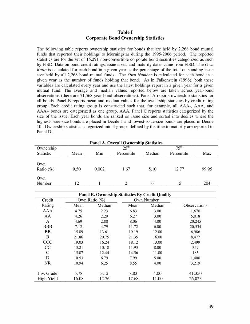
39

Table I

Corporate Bond Ownership Statistics

The following table reports ownership statistics for bonds that are held by 2,268 bond mutual funds that reported their holdings to Morningstar during the 1995-2006 period. The reported statistics are for the set of 15,291 non-convertible corporate bond securities categorized as such by FISD. Data on bond credit ratings, issue sizes, and maturity dates came from FISD. The Own

Ratio is calculated for each bond in a given year as the percentage of the total outstanding issue size held by all 2,268 bond mutual funds. The Own Number is calculated for each bond in a given year as the number of funds holding that bond. As in Falkenstein (1996), both these variables are calculated every year and use the latest holdings report in a given year for a given mutual fund. The average and median values reported below are taken across year-bond observations (there are 71,568 year-bond observations). Panel A reports ownership statistics for all bonds. Panel B reports mean and median values for the ownership statistics by credit rating group. Each credit rating group is constructed such that, for example, all AAA-, AAA, and AAA+ bonds are categorized as one group, AAA. Panel C reports statistics categorized by the size of the issue. Each year bonds are ranked on issue size and sorted into deciles where the highest-issue-size bonds are placed in Decile 1 and lowest-issue-size bonds are placed in Decile 10. Ownership statistics categorized into 4 groups defined by the time to maturity are reported in Panel D.

Panel A. Overall Ownership Statistics

Ownership Statistic

Mean

Min

25th Percentile

Median

75th Percentile

Max

Own Ratio (%) 9.50 0.002 1.67 5.10 12.77 99.95 Own Number 12 1 2 6 15 204

Panel B. Ownership Statistics By Credit Quality

Own Ratio (%) Own Number Credit Rating Mean Median Mean Median Observations

AAA 4.75 2.23 6.83 3.00 1,670 AA 4.26 2.29 6.27 3.00 5,018 A 4.69 2.80 8.06 4.00 20,245

BBB 7.12 4.79 11.72 6.00 20,534 BB 15.89 13.61 19.19 12.00 6,986 B 21.86 20.75 21.35 16.00 8,477

CCC 19.03 16.24 18.12 13.00 2,499 CC 13.21 10.18 11.93 8.00 359 C 15.07 12.44 14.56 11.00 185 D 10.53 6.79 7.99 5.00 1,400

NR 10.94 6.25 8.55 4.00 3,219

Inv. Grade 5.78 3.12 8.83 4.00 41,350 High Yield 16.08 12.76 17.68 11.00 26,023

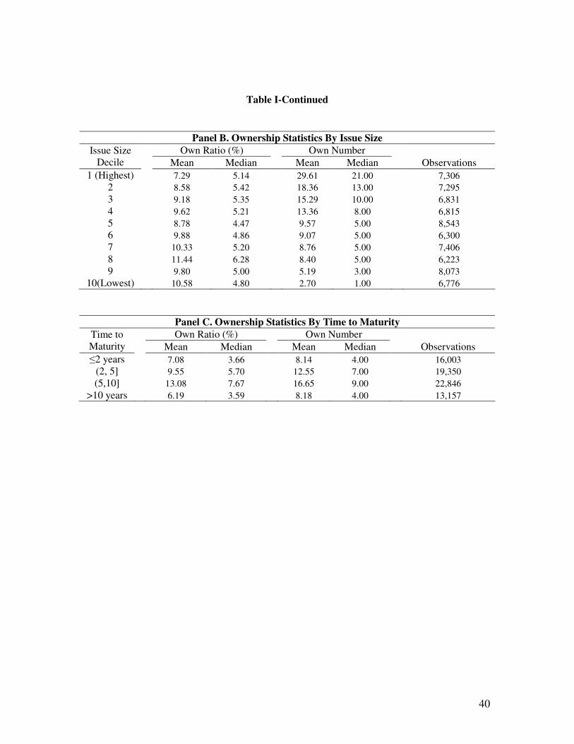
40

Table I-Continued

Panel B. Ownership Statistics By Issue Size

Own Ratio (%) Own Number Issue Size Decile Mean Median Mean Median Observations

1 (Highest) 7.29 5.14 29.61 21.00 7,306 2 8.58 5.42 18.36 13.00 7,295 3 9.18 5.35 15.29 10.00 6,831 4 9.62 5.21 13.36 8.00 6,815 5 8.78 4.47 9.57 5.00 8,543 6 9.88 4.86 9.07 5.00 6,300 7 10.33 5.20 8.76 5.00 7,406 8 11.44 6.28 8.40 5.00 6,223 9 9.80 5.00 5.19 3.00 8,073

10(Lowest) 10.58 4.80 2.70 1.00 6,776

Panel C. Ownership Statistics By Time to Maturity

Own Ratio (%) Own Number Time to Maturity Mean Median Mean Median Observations

≤2 years 7.08 3.66 8.14 4.00 16,003 (2, 5] 9.55 5.70 12.55 7.00 19,350 (5,10] 13.08 7.67 16.65 9.00 22,846

>10 years 6.19 3.59 8.18 4.00 13,157

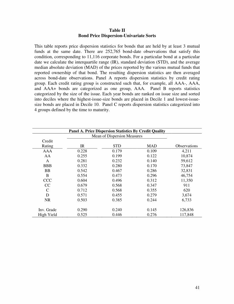
41

Table II

Bond Price Dispersion-Univariate Sorts

This table reports price dispersion statistics for bonds that are held by at least 3 mutual funds at the same date. There are 252,765 bond-date observations that satisfy this condition, corresponding to 11,116 corporate bonds. For a particular bond at a particular date we calculate the interquartile range (IR), standard deviation (STD), and the average median absolute deviation (MAD) of the prices reported by the various mutual funds that reported ownership of that bond. The resulting dispersion statistics are then averaged across bond-date observations. Panel A reports dispersion statistics by credit rating group. Each credit rating group is constructed such that, for example, all AAA-, AAA, and AAA+ bonds are categorized as one group, AAA. Panel B reports statistics categorized by the size of the issue. Each year bonds are ranked on issue size and sorted into deciles where the highest-issue-size bonds are placed in Decile 1 and lowest-issue-size bonds are placed in Decile 10. Panel C reports dispersion statistics categorized into 4 groups defined by the time to maturity.

Panel A. Price Dispersion Statistics By Credit Quality Mean of Dispersion Measures

Credit Rating

IR

STD

MAD

Observations

AAA 0.228 0.179 0.109 4,211 AA 0.255 0.199 0.122 10,874 A 0.281 0.232 0.140 59,612

BBB 0.332 0.280 0.170 73,847 BB 0.542 0.467 0.286 32,831 B 0.554 0.473 0.296 46,754

CCC 0.604 0.496 0.312 11,350 CC 0.679 0.568 0.347 911 C 0.712 0.568 0.355 620 D 0.571 0.455 0.279 3,674

NR 0.503 0.385 0.244 6,733

Inv. Grade 0.290 0.240 0.145 126,836 High Yield 0.525 0.446 0.276 117,848

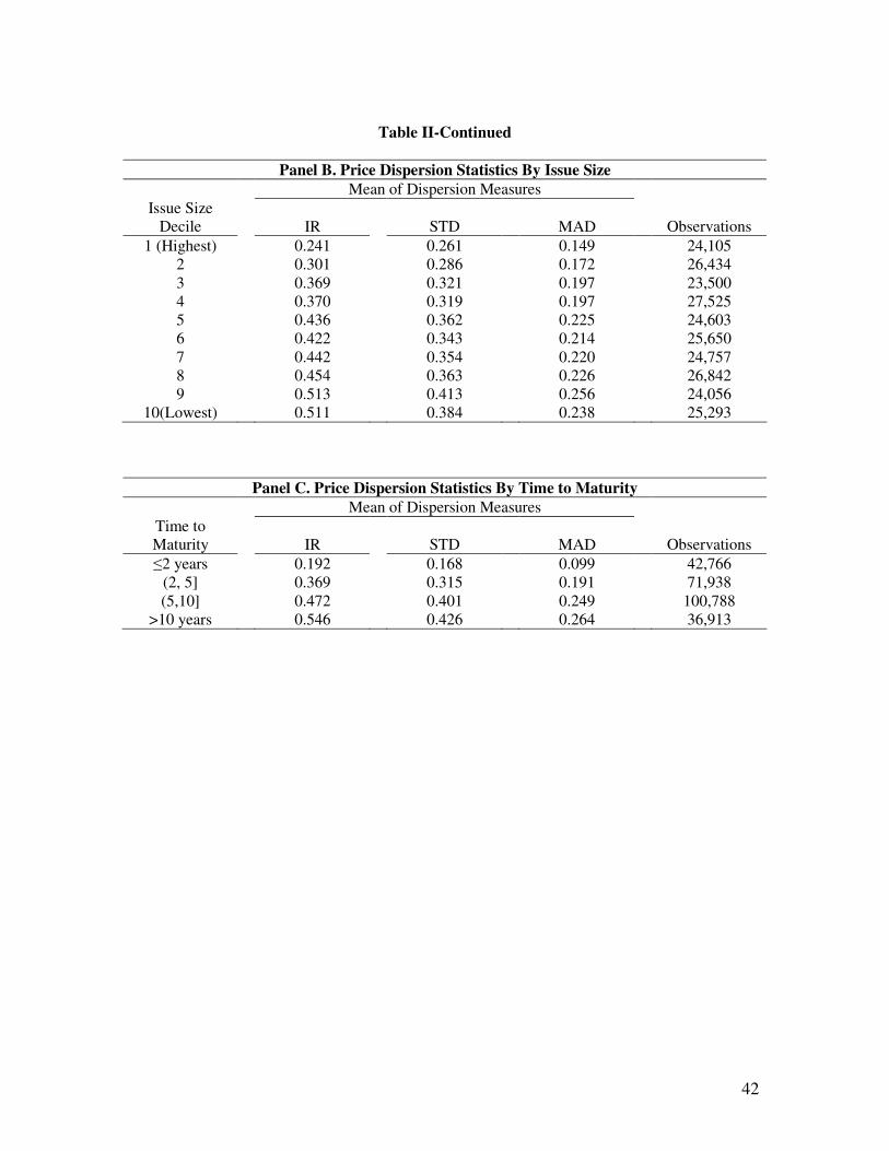
42

Table II-Continued

Panel B. Price Dispersion Statistics By Issue Size

Mean of Dispersion Measures

Issue Size Decile

IR

STD

MAD

Observations

1 (Highest) 0.241 0.261 0.149 24,105 2 0.301 0.286 0.172 26,434 3 0.369 0.321 0.197 23,500 4 0.370 0.319 0.197 27,525 5 0.436 0.362 0.225 24,603 6 0.422 0.343 0.214 25,650 7 0.442 0.354 0.220 24,757 8 0.454 0.363 0.226 26,842 9 0.513 0.413 0.256 24,056

10(Lowest) 0.511 0.384 0.238 25,293

Panel C. Price Dispersion Statistics By Time to Maturity

Mean of Dispersion Measures

Time to Maturity

IR

STD

MAD

Observations

≤2 years 0.192 0.168 0.099 42,766 (2, 5] 0.369 0.315 0.191 71,938 (5,10] 0.472 0.401 0.249 100,788

>10 years 0.546 0.426 0.264 36,913

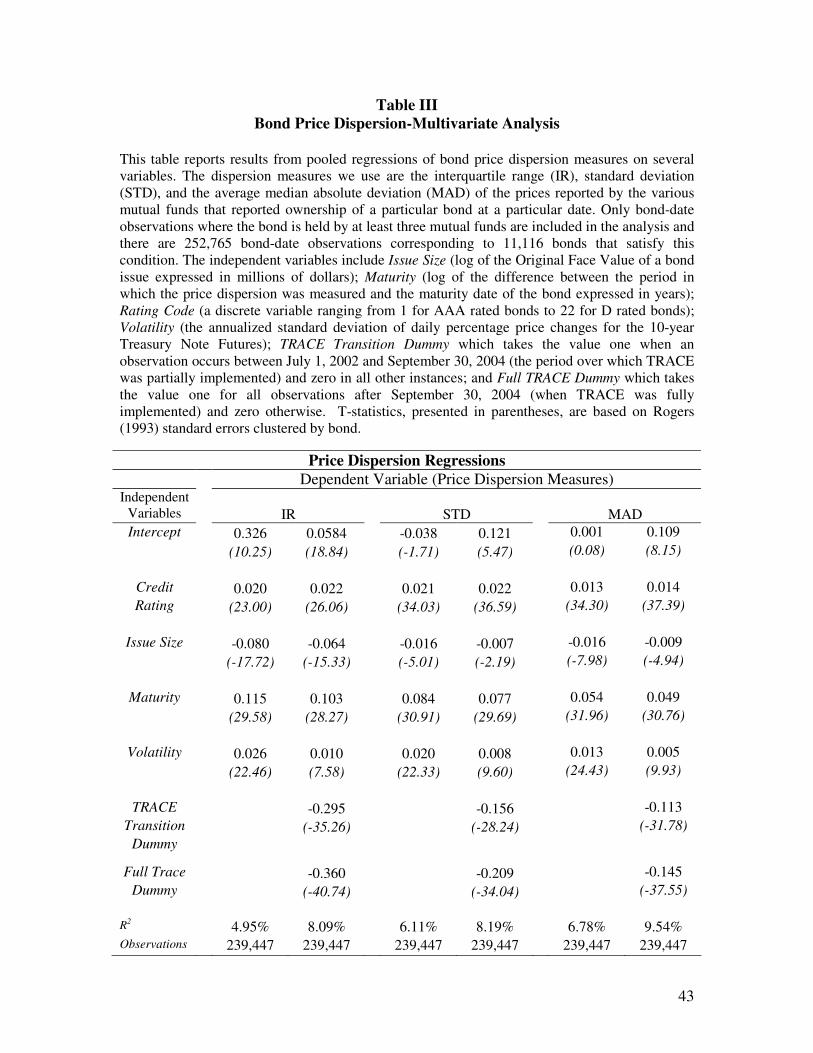
43

Table III

Bond Price Dispersion-Multivariate Analysis

This table reports results from pooled regressions of bond price dispersion measures on several variables. The dispersion measures we use are the interquartile range (IR), standard deviation (STD), and the average median absolute deviation (MAD) of the prices reported by the various mutual funds that reported ownership of a particular bond at a particular date. Only bond-date observations where the bond is held by at least three mutual funds are included in the analysis and there are 252,765 bond-date observations corresponding to 11,116 bonds that satisfy this condition. The independent variables include Issue Size (log of the Original Face Value of a bond issue expressed in millions of dollars); Maturity (log of the difference between the period in which the price dispersion was measured and the maturity date of the bond expressed in years); Rating Code (a discrete variable ranging from 1 for AAA rated bonds to 22 for D rated bonds); Volatility (the annualized standard deviation of daily percentage price changes for the 10-year Treasury Note Futures); TRACE Transition Dummy which takes the value one when an observation occurs between July 1, 2002 and September 30, 2004 (the period over which TRACE was partially implemented) and zero in all other instances; and Full TRACE Dummy which takes the value one for all observations after September 30, 2004 (when TRACE was fully implemented) and zero otherwise. T-statistics, presented in parentheses, are based on Rogers (1993) standard errors clustered by bond.

Price Dispersion Regressions Dependent Variable (Price Dispersion Measures)

Independent Variables

IR

STD

MAD

Intercept 0.326 0.0584 -0.038 0.121 0.001 0.109

(10.25) (18.84) (-1.71) (5.47) (0.08) (8.15)

Credit 0.020 0.022 0.021 0.022 0.013 0.014

Rating (23.00) (26.06) (34.03) (36.59) (34.30) (37.39)

Issue Size -0.080 -0.064 -0.016 -0.007 -0.016 -0.009

(-17.72) (-15.33) (-5.01) (-2.19) (-7.98) (-4.94)

Maturity 0.115 0.103 0.084 0.077 0.054 0.049

(29.58) (28.27) (30.91) (29.69) (31.96) (30.76)

Volatility 0.026 0.010 0.020 0.008 0.013 0.005

(22.46) (7.58) (22.33) (9.60) (24.43) (9.93)

TRACE -0.295 -0.156 -0.113

Transition (-35.26) (-28.24) (-31.78)

Dummy

Full Trace -0.360 -0.209 -0.145

Dummy (-40.74) (-34.04) (-37.55)

R2 4.95% 8.09% 6.11% 8.19% 6.78% 9.54% Observations 239,447 239,447 239,447 239,447 239,447 239,447

44

Table IV

TRACE Regressions

This table reports results from pooled regressions of bond price dispersion measures on several control variables and certain dummy variables created to capture the impact of TRACE on the dispersion of bond prices. The dispersion measures we use are the interquartile range (IR), standard deviation (STD), and average median absolute deviation (MAD) of the prices reported by the various mutual funds that reported ownership of a particular bond at a particular date. Only bond-date observations where the bond is held by at least three mutual funds are included in the analysis and there are 252,765 bond-date observations corresponding to 11,116 bonds that satisfy this condition. The control variables include Issue Size (log of the Original Face Value of a bond issue expressed in millions of dollars); Maturity (log of the difference between the period in which the price dispersion was measured and the maturity date of the bond expressed in years); Rating Code (a discrete variable ranging from 1 for AAA rated bonds to 22 for D rated bonds); and Volatility (the annualized standard deviation of daily percentage price changes for the 10-year Treasury Note Futures). The Set I specification includes all bonds conforming to the set of bonds that became permanently TRACE-eligible as of July 1, 2002 (all investment grade bonds greater than $1 billion in original issue size). The Set II specification includes all bonds conforming to the set of bonds that became permanently TRACE-eligible as of March, 2003 (all investment grade bonds rated A or higher with original issue size of $100 million or greater). Both Set I and II specifications are reported in Panel A. The remaining specification in Panel B includes all bonds with characteristics other than those shared by the bonds in Set I and II. The TRACE

Eligible Dummy used in the Panel B equals one when a particular bond had a TRACE trade report during the July 1, 2002- September 30, 2004 period and zero in all the other instances. The TRACE Ineligible Dummy takes the value one if a bond did not have a TRACE trade report during the July 1, 2002- September 30, 2004 period and zero in all the other instances. The Full

TRACE Dummy is one for all observations after September 30, 2004 (after which TRACE was fully implemented) and zero otherwise. The F-test in Panel B is based on the null hypothesis that the coefficients for TRACE Eligible and TRACE Ineligible Dummies are equal. T-statistics, presented in parentheses, are based on Rogers (1993) standard errors clustered by bond.

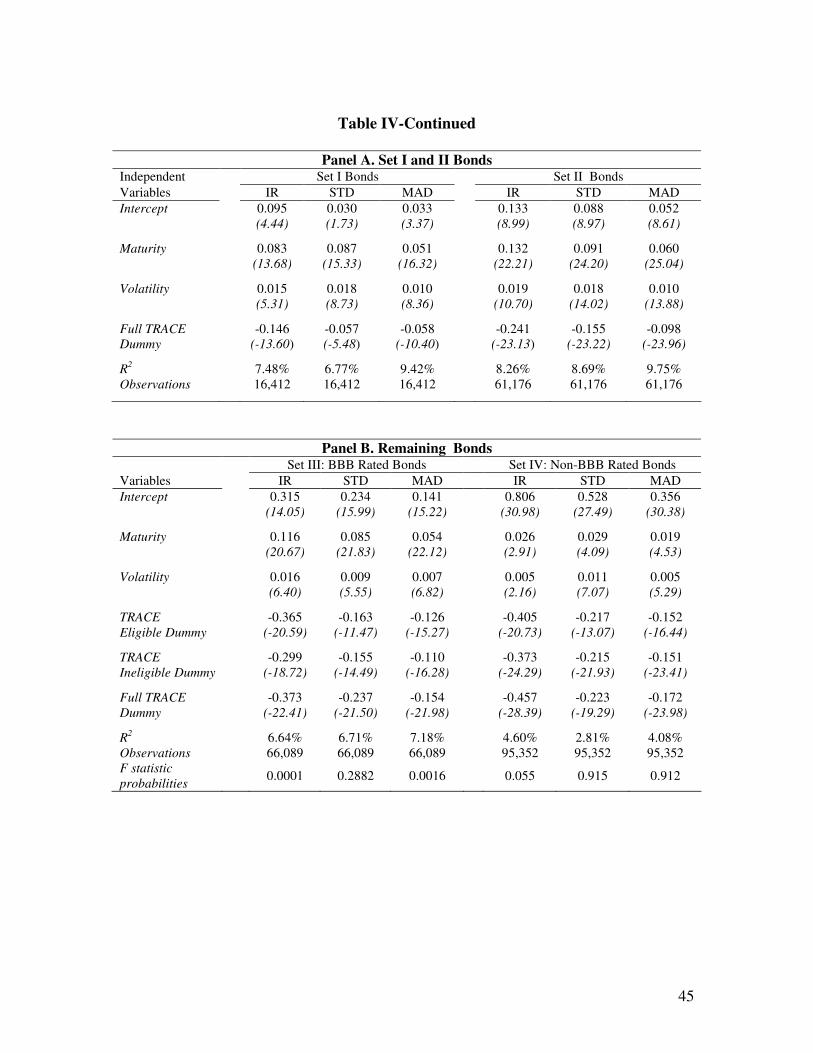
45

Table IV-Continued

Panel A. Set I and II Bonds

Independent Set I Bonds Set II Bonds

Variables IR STD MAD IR STD MAD

Intercept 0.095 0.030 0.033 0.133 0.088 0.052 (4.44) (1.73) (3.37) (8.99) (8.97) (8.61)

Maturity 0.083 0.087 0.051 0.132 0.091 0.060 (13.68) (15.33) (16.32) (22.21) (24.20) (25.04)

Volatility 0.015 0.018 0.010 0.019 0.018 0.010 (5.31) (8.73) (8.36) (10.70) (14.02) (13.88)

Full TRACE -0.146 -0.057 -0.058 -0.241 -0.155 -0.098 Dummy (-13.60) (-5.48) (-10.40) (-23.13) (-23.22) (-23.96)

R

2 7.48% 6.77% 9.42% 8.26% 8.69% 9.75%

Observations 16,412 16,412 16,412 61,176 61,176 61,176

Panel B. Remaining Bonds

Set III: BBB Rated Bonds Set IV: Non-BBB Rated Bonds

Variables IR STD MAD IR STD MAD

Intercept 0.315 0.234 0.141 0.806 0.528 0.356 (14.05) (15.99) (15.22) (30.98) (27.49) (30.38)

Maturity 0.116 0.085 0.054 0.026 0.029 0.019 (20.67) (21.83) (22.12) (2.91) (4.09) (4.53)

Volatility 0.016 0.009 0.007 0.005 0.011 0.005 (6.40) (5.55) (6.82) (2.16) (7.07) (5.29)

TRACE -0.365 -0.163 -0.126 -0.405 -0.217 -0.152 Eligible Dummy (-20.59) (-11.47) (-15.27) (-20.73) (-13.07) (-16.44)

TRACE -0.299 -0.155 -0.110 -0.373 -0.215 -0.151 Ineligible Dummy (-18.72) (-14.49) (-16.28) (-24.29) (-21.93) (-23.41)

Full TRACE -0.373 -0.237 -0.154 -0.457 -0.223 -0.172 Dummy (-22.41) (-21.50) (-21.98) (-28.39) (-19.29) (-23.98)

R

2 6.64% 6.71% 7.18% 4.60% 2.81% 4.08%

Observations 66,089 66,089 66,089 95,352 95,352 95,352 F statistic

probabilities

0.0001 0.2882 0.0016 0.055 0.915 0.912

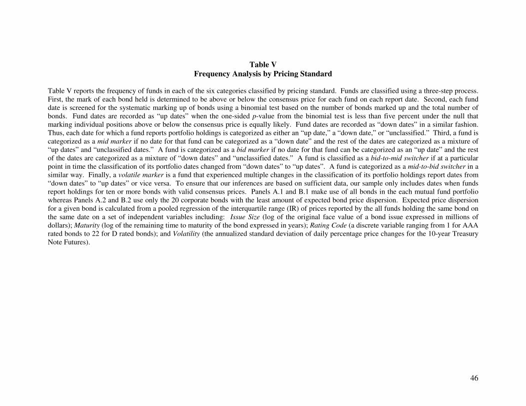
46

Table V

Frequency Analysis by Pricing Standard

Table V reports the frequency of funds in each of the six categories classified by pricing standard. Funds are classified using a three-step process. First, the mark of each bond held is determined to be above or below the consensus price for each fund on each report date. Second, each fund date is screened for the systematic marking up of bonds using a binomial test based on the number of bonds marked up and the total number of bonds. Fund dates are recorded as “up dates” when the one-sided p-value from the binomial test is less than five percent under the null that marking individual positions above or below the consensus price is equally likely. Fund dates are recorded as “down dates” in a similar fashion. Thus, each date for which a fund reports portfolio holdings is categorized as either an “up date,” a “down date,” or “unclassified.” Third, a fund is categorized as a mid marker if no date for that fund can be categorized as a “down date” and the rest of the dates are categorized as a mixture of “up dates” and “unclassified dates.” A fund is categorized as a bid marker if no date for that fund can be categorized as an “up date” and the rest of the dates are categorized as a mixture of “down dates” and “unclassified dates.” A fund is classified as a bid-to-mid switcher if at a particular point in time the classification of its portfolio dates changed from “down dates” to “up dates”. A fund is categorized as a mid-to-bid switcher in a similar way. Finally, a volatile marker is a fund that experienced multiple changes in the classification of its portfolio holdings report dates from “down dates” to “up dates” or vice versa. To ensure that our inferences are based on sufficient data, our sample only includes dates when funds report holdings for ten or more bonds with valid consensus prices. Panels A.1 and B.1 make use of all bonds in the each mutual fund portfolio whereas Panels A.2 and B.2 use only the 20 corporate bonds with the least amount of expected bond price dispersion. Expected price dispersion for a given bond is calculated from a pooled regression of the interquartile range (IR) of prices reported by the all funds holding the same bond on the same date on a set of independent variables including: Issue Size (log of the original face value of a bond issue expressed in millions of dollars); Maturity (log of the remaining time to maturity of the bond expressed in years); Rating Code (a discrete variable ranging from 1 for AAA rated bonds to 22 for D rated bonds); and Volatility (the annualized standard deviation of daily percentage price changes for the 10-year Treasury Note Futures).

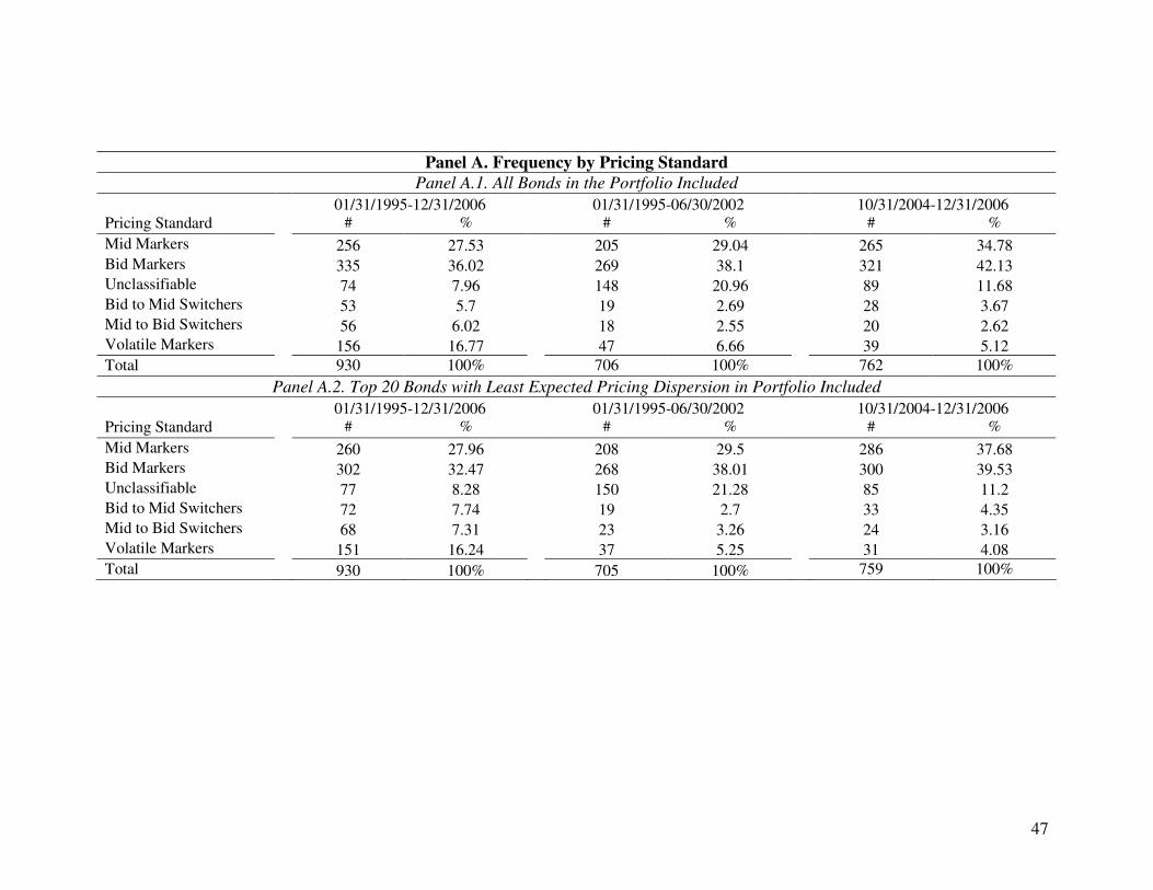
47

Panel A. Frequency by Pricing Standard

Panel A.1. All Bonds in the Portfolio Included

01/31/1995-12/31/2006 01/31/1995-06/30/2002 10/31/2004-12/31/2006 Pricing Standard # % # % # %

Mid Markers 256 27.53 205 29.04 265 34.78 Bid Markers 335 36.02 269 38.1 321 42.13 Unclassifiable 74 7.96 148 20.96 89 11.68 Bid to Mid Switchers 53 5.7 19 2.69 28 3.67 Mid to Bid Switchers 56 6.02 18 2.55 20 2.62 Volatile Markers 156 16.77 47 6.66 39 5.12

Total 930 100% 706 100% 762 100%

Panel A.2. Top 20 Bonds with Least Expected Pricing Dispersion in Portfolio Included

01/31/1995-12/31/2006 01/31/1995-06/30/2002 10/31/2004-12/31/2006 Pricing Standard # % # % # %

Mid Markers 260 27.96 208 29.5 286 37.68 Bid Markers 302 32.47 268 38.01 300 39.53 Unclassifiable 77 8.28 150 21.28 85 11.2 Bid to Mid Switchers 72 7.74 19 2.7 33 4.35 Mid to Bid Switchers 68 7.31 23 3.26 24 3.16 Volatile Markers 151 16.24 37 5.25 31 4.08

Total 930 100% 705 100% 759 100%

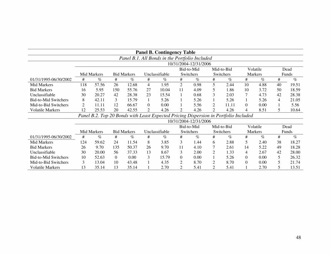
48

Panel B. Contingency Table

Panel B.1. All Bonds in the Portfolio Included

10/31/2004-12/31/2006

Mid Markers

Bid Markers

Unclassifiable

Bid-to-Mid Switchers

Mid-to-Bid Switchers

Volatile Markers

Dead Funds

01/31/1995-06/30/2002 # % # % # % # % # % # % # %

Mid Markers 118 57.56 26 12.68 4 1.95 2 0.98 5 2.44 10 4.88 40 19.51 Bid Markers 16 5.95 150 55.76 27 10.04 11 4.09 5 1.86 10 3.72 50 18.59 Unclassifiable 30 20.27 42 28.38 23 15.54 1 0.68 3 2.03 7 4.73 42 28.38 Bid-to-Mid Switchers 8 42.11 3 15.79 1 5.26 1 5.26 1 5.26 1 5.26 4 21.05 Mid-to-Bid Switchers 2 11.11 12 66.67 0 0.00 1 5.56 2 11.11 0 0.00 1 5.56 Volatile Markers 12 25.53 20 42.55 2 4.26 2 4.26 2 4.26 4 8.51 5 10.64

Panel B.2. Top 20 Bonds with Least Expected Pricing Dispersion in Portfolio Included

10/31/2004-12/31/2006

Mid Markers

Bid Markers

Unclassifiable

Bid-to-Mid Switchers

Mid-to-Bid Switchers

Volatile Markers

Dead Funds

01/31/1995-06/30/2002 # % # % # % # % # % # % # %

Mid Markers 124 59.62 24 11.54 8 3.85 3 1.44 6 2.88 5 2.40 38 18.27 Bid Markers 26 9.70 135 50.37 26 9.70 11 4.10 7 2.61 14 5.22 49 18.28 Unclassifiable 30 20.00 56 37.33 13 8.67 3 2.00 2 1.33 4 2.67 42 28.00 Bid-to-Mid Switchers 10 52.63 0 0.00 3 15.79 0 0.00 1 5.26 0 0.00 5 26.32 Mid-to-Bid Switchers 3 13.04 10 43.48 1 4.35 2 8.70 2 8.70 0 0.00 5 21.74 Volatile Markers 13 35.14 13 35.14 1 2.70 2 5.41 2 5.41 1 2.70 5 13.51

49

Table VI

Price Dispersion Computed Holding Pricing Standard Constant

This table reports results from pooled regressions of bond price dispersion measures (IR, STD, MAD) on control variables and Trace dummy variables as specified in Table IV. The price dispersion statistics in Panels A and B are based on all bond prices reported by presumed mid-

marking funds and presumed bid-marking funds, respectively. Funds are classified as presumed

mid-marking or bid-marking using a three-step process. First, for each fund each portfolio date, the mark of each bond held is determined to be above or below the consensus price. Second, each fund date is screened for the systematic marking up of bonds using a binomial test based on the number of bonds marked up and the total number of bonds. Fund dates are recorded as “up dates” when the one-sided p-value from the binomial test is less than five percent under the null that marking individual positions above or below the consensus price is equally likely. Fund dates are recorded as “down dates” in a similar fashion. Thus, each date for which a fund reports portfolio holdings is categorized as either an “up date,” a “down date,” or “unclassified.” Third, a fund is categorized as a presumed mid-marker if at least one of the portfolio dates for that fund is categorized as an “up date” and the rest of the dates are categorized as “unclassified.” A fund is categorized as a presumed bid marker if at least one of the portfolio dates for that fund is categorized as a “down date” and the rest of the dates are categorized as “unclassified.” To ensure that our inferences are based on sufficient data, our sample only includes months when funds report holdings for ten or more bonds with valid consensus prices. T-statistics, presented in parentheses, are based on Rogers (1993) standard errors clustered by bond.

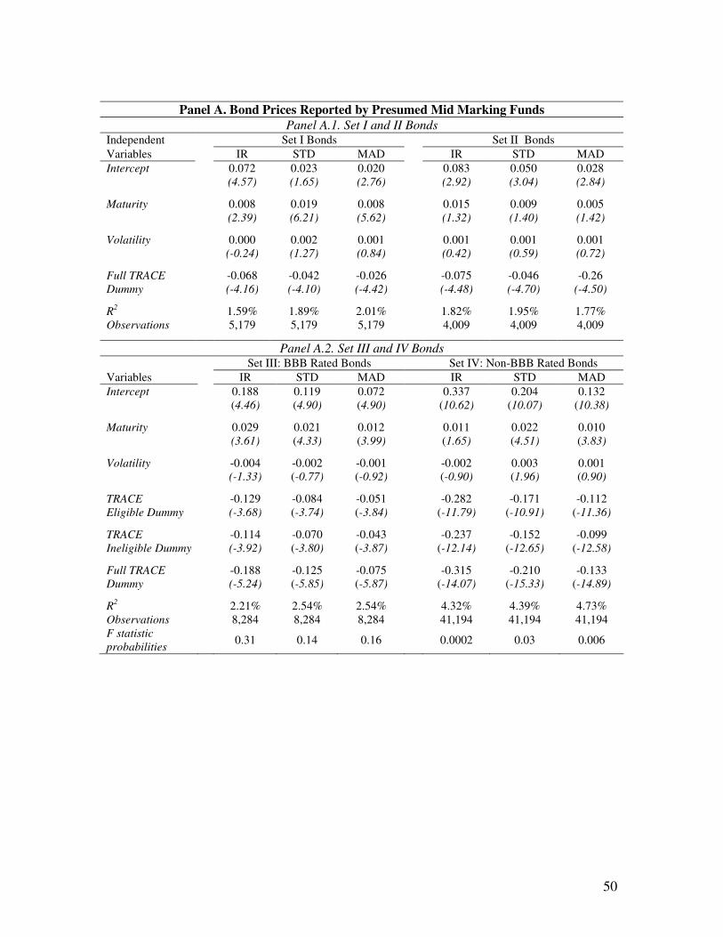
50

Panel A. Bond Prices Reported by Presumed Mid Marking Funds

Panel A.1. Set I and II Bonds Independent Set I Bonds Set II Bonds

Variables IR STD MAD IR STD MAD

Intercept 0.072 0.023 0.020 0.083 0.050 0.028 (4.57) (1.65) (2.76) (2.92) (3.04) (2.84)

Maturity 0.008 0.019 0.008 0.015 0.009 0.005 (2.39) (6.21) (5.62) (1.32) (1.40) (1.42)

Volatility 0.000 0.002 0.001 0.001 0.001 0.001 (-0.24) (1.27) (0.84) (0.42) (0.59) (0.72)

Full TRACE -0.068 -0.042 -0.026 -0.075 -0.046 -0.26 Dummy (-4.16) (-4.10) (-4.42) (-4.48) (-4.70) (-4.50)

R

2 1.59% 1.89% 2.01% 1.82% 1.95% 1.77%

Observations 5,179 5,179 5,179 4,009 4,009 4,009

Panel A.2. Set III and IV Bonds Set III: BBB Rated Bonds Set IV: Non-BBB Rated Bonds

Variables IR STD MAD IR STD MAD

Intercept 0.188 0.119 0.072 0.337 0.204 0.132 (4.46) (4.90) (4.90) (10.62) (10.07) (10.38)

Maturity 0.029 0.021 0.012 0.011 0.022 0.010 (3.61) (4.33) (3.99) (1.65) (4.51) (3.83)

Volatility -0.004 -0.002 -0.001 -0.002 0.003 0.001 (-1.33) (-0.77) (-0.92) (-0.90) (1.96) (0.90)

TRACE -0.129 -0.084 -0.051 -0.282 -0.171 -0.112 Eligible Dummy (-3.68) (-3.74) (-3.84) (-11.79) (-10.91) (-11.36)

TRACE -0.114 -0.070 -0.043 -0.237 -0.152 -0.099 Ineligible Dummy (-3.92) (-3.80) (-3.87) (-12.14) (-12.65) (-12.58)

Full TRACE -0.188 -0.125 -0.075 -0.315 -0.210 -0.133 Dummy (-5.24) (-5.85) (-5.87) (-14.07) (-15.33) (-14.89)

R

2 2.21% 2.54% 2.54% 4.32% 4.39% 4.73%

Observations 8,284 8,284 8,284 41,194 41,194 41,194 F statistic

probabilities

0.31 0.14 0.16 0.0002 0.03 0.006

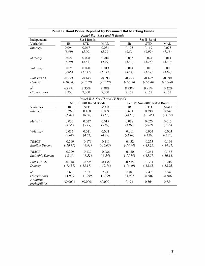
51

Panel B. Bond Prices Reported by Presumed Bid Marking Funds

Panel B.1. Set I and II Bonds Independent Set I Bonds Set II Bonds

Variables IR STD MAD IR STD MAD

Intercept 0.094 0.047 0.031 0.195 0.119 0.073 (3.99) (3.00) (3.26) (6.84) (6.99) (7.13)

Maturity 0.027 0.028 0.016 0.035 0.024 0.014 (3.79) (5.32) (4.99) (3.30) (3.76) (3.50)

Volatility 0.026 0.020 0.013 0.014 0.010 0.006 (9.06) (11.17) (11.12) (4.54) (5.57) (5.67)

Full TRACE -0.223 -0.140 -0.093 -0.253 -0.162 -0.099 Dummy (-10.34) (-10.18) (-10.29) (-12.26) (-12.90) (-13.04)

R

2 6.99% 8.35% 8.38% 8.73% 9.91% 10.22%

Observations 7,350 7,350 7,350 7,152 7,152 7,152

Panel B.2. Set III and IV Bonds Set III: BBB Rated Bonds Set IV: Non-BBB Rated Bonds

Variables IR STD MAD IR STD MAD

Intercept 0.260 0.168 0.099 0.631 0.390 0.242 (5.82) (6.08) (5.58) (14.52) (13.85) (14.12)

Maturity 0.033 0.027 0.015 0.018 0.026 0.015 (4.55) (5.49) (5.07) (1.91) (4.02) (3.75)

Volatility 0.017 0.011 0.008 -0.011 -0.004 -0.003 (3.69) (4.01) (4.29) (-3.16) (-1.82) (-2.20)

TRACE -0.299 -0.179 -0.111 -0.452 -0.253 -0.166 Eligible Dummy (-10.71) (-9.91) (-10.05) (-14.94) (-13.25) (-14.41)

TRACE -0.229 -0.139 -0.086 -0.430 -0.261 -0.167 Ineligible Dummy (-8.69) (-8.52) (-8.54) (-15.74) (-15.57) (-16.18)

Full TRACE -0.348 -0.228 -0.138 -0.535 -0.334 -0.210 Dummy (-12.57) (-13.11) (-12.78) (-18.49) (-18.45) (-18.93)

R

2 6.63 7.37 7.21 8.04 7.47 8.54

Observations 11,999 11,999 11,999 31,907 31,907 31,907 F statistic

probabilities

<0.0001 <0.0001 <0.0001 0.124 0.364 0.854

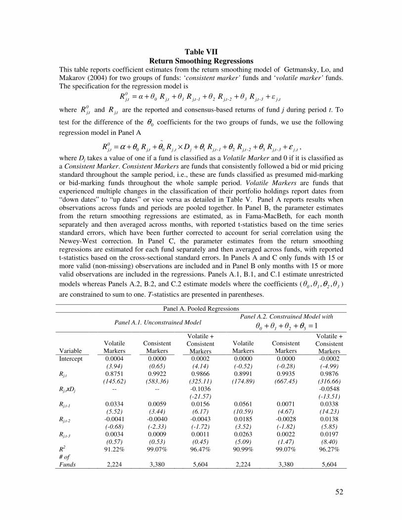
52

Table VII

Return Smoothing Regressions This table reports coefficient estimates from the return smoothing model of Getmansky, Lo, and Makarov (2004) for two groups of funds: ‘consistent marker’ funds and ‘volatile marker’ funds. The specification for the regression model is

tj3-tj,32-tj,21-tj,1tj,0

0

tj, εR θR θR θR θαR ,+++++=

where 0

tj,R and tj,R are the reported and consensus-based returns of fund j during period t. To

test for the difference of the 0θ coefficients for the two groups of funds, we use the following

regression model in Panel A

tj3-tj,2-tj,1-tj,jtjtj,

0

tj, R R R DRR R ,321,

~

00 εθθθθθα ++++×++= ,

where Dj takes a value of one if a fund is classified as a Volatile Marker and 0 if it is classified as a Consistent Marker. Consistent Markers are funds that consistently followed a bid or mid pricing standard throughout the sample period, i.e., these are funds classified as presumed mid-marking or bid-marking funds throughout the whole sample period. Volatile Markers are funds that experienced multiple changes in the classification of their portfolio holdings report dates from “down dates” to “up dates” or vice versa as detailed in Table V. Panel A reports results when observations across funds and periods are pooled together. In Panel B, the parameter estimates from the return smoothing regressions are estimated, as in Fama-MacBeth, for each month separately and then averaged across months, with reported t-statistics based on the time series standard errors, which have been further corrected to account for serial correlation using the Newey-West correction. In Panel C, the parameter estimates from the return smoothing regressions are estimated for each fund separately and then averaged across funds, with reported t-statistics based on the cross-sectional standard errors. In Panels A and C only funds with 15 or more valid (non-missing) observations are included and in Panel B only months with 15 or more valid observations are included in the regressions. Panels A.1, B.1, and C.1 estimate unrestricted

models whereas Panels A.2, B.2, and C.2 estimate models where the coefficients ( 3210 θ, ,θ ,θ θ )

are constrained to sum to one. T-statistics are presented in parentheses.

Panel A. Pooled Regressions

Panel A.1. Unconstrained Model

Panel A.2. Constrained Model with

13 =+++ θ210 θ θθ

Variable

Volatile Markers

Consistent Markers

Volatile + Consistent Markers

Volatile Markers

Consistent Markers

Volatile + Consistent Markers

Intercept 0.0004 0.0000 0.0002 0.0000 0.0000 -0.0002 (3.94) (0.65) (4.14) (-0.52) (-0.28) (-4.99)

Rj,t 0.8751 0.9922 0.9866 0.8991 0.9935 0.9876 (145.62) (583.36) (325.11) (174.89) (667.45) (316.66)

Rj,txDj -- -- -0.1036 -0.0548 (-21.57) (-13.51) Rj,t-1 0.0334 0.0059 0.0156 0.0561 0.0071 0.0338 (5.52) (3.44) (6.17) (10.59) (4.67) (14.23) Rj,t-2 -0.0041 -0.0040 -0.0043 0.0185 -0.0028 0.0138 (-0.68) (-2.33) (-1.72) (3.52) (-1.82) (5.85) Rj,t-3 0.0034 0.0009 0.0011 0.0263 0.0022 0.0197 (0.57) (0.53) (0.45) (5.09) (1.47) (8.40) R

2 91.22% 99.07% 96.47% 90.99% 99.07% 96.27%

# of

Funds

2,224 3,380 5,604 2,224 3,380 5,604

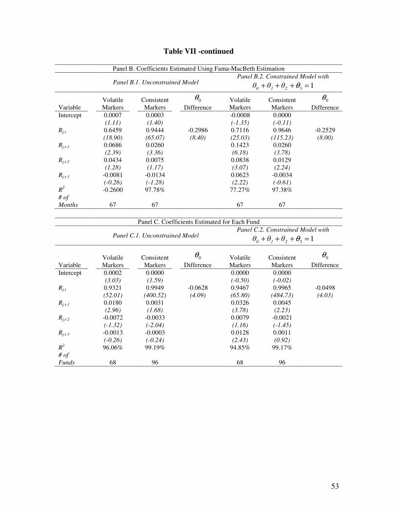
53

Table VII -continued

Panel B. Coefficients Estimated Using Fama-MacBeth Estimation

Panel B.1. Unconstrained Model

Panel B.2. Constrained Model with

13 =+++ θ210 θ θθ

Variable

Volatile Markers

Consistent Markers

0θ

Difference

Volatile Markers

Consistent Markers

0θ

Difference Intercept 0.0007 0.0003 -0.0008 0.0000 (1.11) (1.40) (-1.35) (-0.11)

Rj,t 0.6459 0.9444 -0.2986 0.7116 0.9646 -0.2529 (18.90) (65.07) (8.40) (25.03) (115.23) (8.00)

Rj,t-1 0.0686 0.0260 0.1423 0.0260 (2.39) (3.36) (6.18) (3.78) Rj,t-2 0.0434 0.0075 0.0838 0.0129 (1.28) (1.17) (3.07) (2.24) Rj,t-3 -0.0081 -0.0134 0.0623 -0.0034 (-0.26) (-1.28) (2.22) (-0.61) R

2 -0.2600 97.78% 77.27% 97.38%

# of

Months

67

67

67

67

Panel C. Coefficients Estimated for Each Fund

Panel C.1. Unconstrained Model

Panel C.2. Constrained Model with

13 =+++ θ210 θ θθ

Variable

Volatile Markers

Consistent Markers

0θ

Difference

Volatile Markers

Consistent Markers

0θ

Difference

Intercept 0.0002 0.0000 0.0000 0.0000 (3.03) (1.59) (-0.50) (-0.02)

Rj,t 0.9321 0.9949 -0.0628 0.9467 0.9965 -0.0498 (52.01) (400.52) (4.09) (65.80) (484.73) (4.03)

Rj,t-1 0.0180 0.0031 0.0326 0.0045 (2.96) (1.68) (3.78) (2.23) Rj,t-2 -0.0072 -0.0033 0.0079 -0.0021 (-1.32) (-2.04) (1.16) (-1.45) Rj,t-3 -0.0013 -0.0003 0.0128 0.0011 (-0.26) (-0.24) (2.43) (0.92) R

2 96.06% 99.19% 94.85% 99.17%

# of

Funds

68 96 68 96

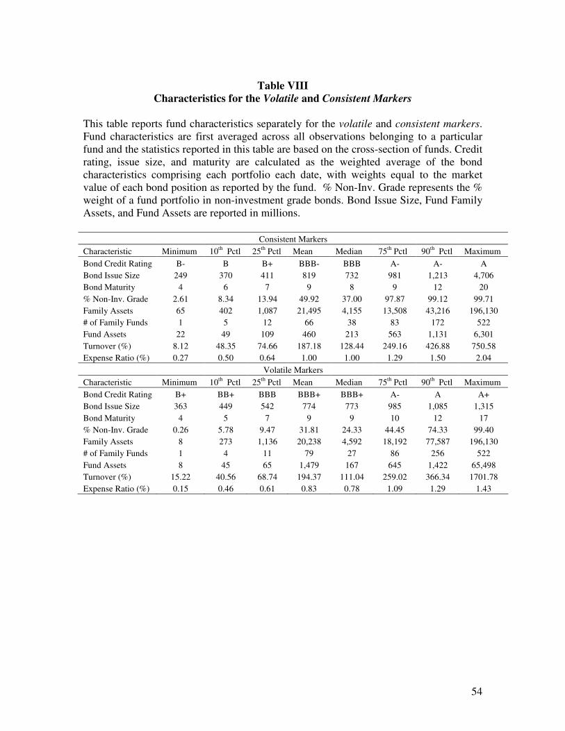
54

Table VIII

Characteristics for the Volatile and Consistent Markers

This table reports fund characteristics separately for the volatile and consistent markers. Fund characteristics are first averaged across all observations belonging to a particular fund and the statistics reported in this table are based on the cross-section of funds. Credit rating, issue size, and maturity are calculated as the weighted average of the bond characteristics comprising each portfolio each date, with weights equal to the market value of each bond position as reported by the fund. % Non-Inv. Grade represents the % weight of a fund portfolio in non-investment grade bonds. Bond Issue Size, Fund Family Assets, and Fund Assets are reported in millions.

Consistent Markers

Characteristic Minimum 10th Pctl 25

th Pctl Mean Median 75

th Pctl 90

th Pctl Maximum

Bond Credit Rating B- B B+ BBB- BBB A- A- A

Bond Issue Size 249 370 411 819 732 981 1,213 4,706

Bond Maturity 4 6 7 9 8 9 12 20

% Non-Inv. Grade 2.61 8.34 13.94 49.92 37.00 97.87 99.12 99.71

Family Assets 65 402 1,087 21,495 4,155 13,508 43,216 196,130

# of Family Funds 1 5 12 66 38 83 172 522

Fund Assets 22 49 109 460 213 563 1,131 6,301

Turnover (%) 8.12 48.35 74.66 187.18 128.44 249.16 426.88 750.58

Expense Ratio (%) 0.27 0.50 0.64 1.00 1.00 1.29 1.50 2.04

Volatile Markers

Characteristic Minimum 10th Pctl 25

th Pctl Mean Median 75

th Pctl 90

th Pctl Maximum

Bond Credit Rating B+ BB+ BBB BBB+ BBB+ A- A A+

Bond Issue Size 363 449 542 774 773 985 1,085 1,315

Bond Maturity 4 5 7 9 9 10 12 17

% Non-Inv. Grade 0.26 5.78 9.47 31.81 24.33 44.45 74.33 99.40

Family Assets 8 273 1,136 20,238 4,592 18,192 77,587 196,130

# of Family Funds 1 4 11 79 27 86 256 522

Fund Assets 8 45 65 1,479 167 645 1,422 65,498

Turnover (%) 15.22 40.56 68.74 194.37 111.04 259.02 366.34 1701.78

Expense Ratio (%) 0.15 0.46 0.61 0.83 0.78 1.09 1.29 1.43

55

REFERENCES

Agarwal, V., and N. Naik, 2000, Multi-period performance persistence analysis of hedge funds, Journal of Financial and Quantitative Analysis 35 (3), 327-342. Agarwal, V., N. Daniel, and N. Naik, 2005, Why is Santa Claus so kind to hedge funds? The December bonanza puzzle! Unpublished working paper. Amihud, Y., H. Mendelson, and B. Lauterbach, 1997, Market microstructure and securities values: Evidence from the Tel Aviv Stock Exchange, Journal of Financial Economics 45, 365-390. Asness, C., R. Krail, and J. Liew, 2001, Do hedge funds hedge? Journal of Portfolio Management 28 (1), 6-19. Bessembinder, H., W. Maxwell, and K. Venkataraman, 2006, Market transparency, liquidity externalities, and institutional trading costs in corporate bonds, Journal of Financial Economics 82 (2), 251-288. Bhargava, R., A. Bose, and D. Dubofsky, 1998, Exploiting international stock market correlations with open-end international mutual funds, Journal of Business, Finance, and Accounting 25, 765-773. Biaisa, B., L. Glosten, and C. Spatt, 2005, Market microstructure: A survey of microfoundations, empirical results, and policy implications, Journal of Financial Markets 8 (2) 217-264. Bloomfield, R. and M. O’Hara, 1999, Market transparency: Who wins and who loses? Review of Financial Studies 12, 5-35. Bollen, N. and V. Pool, 2006, Conditional return smoothing in the hedge fund industry, Journal of Financial and Quantitative Analysis, forthcoming. Bollen, N. and V. Pool, 2007, Do hedge fund managers misreport returns? Evidence from the pooled distribution, Unpublished working paper. Boudoukh, J., M. Richardson, M. Subrahmanyam, and R. Whitelaw, 2002, Stale prices and strategies for trading mutual funds, Financial Analysts Journal 58, 53-71. Chalmers, J., R. Edelen, G. Kadlec, 2001, On the perils of financial intermediaries setting securities prices: the mutual fund wild card option, Journal of Finance 56 (6), 2209-2236. Edwards, A., L. Harris, and M. Piwowar, 2007, Corporate bond market transparency and transaction costs, Journal of Finance 62 (3), 1421–1451.

56

Fama, E., and J. MacBeth, 1973, Risk, return and equilibrium: Empirical tests, Journal of Political Economy 81, 607-636. Getmansky, M., A. Lo, and I. Makarov, 2004, An econometric model of serial correlation and illiquidity in hedge fund returns, Journal of Financial Economics 74, 529-610. Goetzmann, W., Z. Ivkovic, and K. Rouwenhorst, 2001, Day trading international mutual funds: Evidence and policy solutions, Journal of Financial and Quantitative Analysis 36, 287-309. Goldstein, M., E. Hotchkiss, and E. Sirri, 2007, Transparency and liquidity: a controlled experiment on corporate bonds, Review of Financial Studies 20 (2), 235-273 Green, J., and C. Hodges, 2002, The dilution impact of daily fund flows on open-end mutual funds, Journal of Financial Economics 65, 131-158. Investment Company Institute, ICI Mutual Insurance Company and the Independent Directors Council, An introduction to fair valuation, Spring 2005 Madhavan, A., 2000, Market microstructure, Journal of Financial Markets 3, 205–258. Naik, N., A. Neuberger, and S. Viswanathan, 1999, Trade disclosure regulation in markets with negotiated trades, Review of Financial Studies 12 (4), 873-900. Nelson, Matt. Evaluated security pricing services offerings have increased recently. Advanced Trading, March 23, 2007, available at http://www.advancedtrading.com/showArticle.jhtml;jsessionid=T0ABWVMTEFC1YQSNDLRCKH0CJUNN2JVN?articleID=198500315 Newey, W., and K. West, 1994, Automatic lag selection in covariance matrix estimation, The Review of Economic Studies, 61 (4), 631–653; Pagano, M., and A. Roell, 1996, Transparency and liquidity: A comparison of auction and dealer markets with informed trading, Journal of Finance 51, 579-611. Petersen, M., 2008, Estimating standard errors in finance panel data sets: Comparing approaches, Review of Financial Studies, forthcoming PricewaterhouseCoopers LLP, Pricing and Valuation: Risks, Controls and Emerging Practices for Registered Investment Companies, Undated. Pulliam, Susan, Randall Smith, and Michael Siconolf, 2007, U.S. investors face an age of murky pricing, The Wall Street Journal, October 12, A1. Pulliam, Susan, 2007, Bonds’ pricing is questioned in email trail, The Wall Street Journal, October 26, C1.

57

Rahl, L., 2001, Capital market risk advisors NAV/fair value practices survey results, The Journal of Alternative Investments, 4 (3), 55-58. Rogers, W., 1993, Regression standard errors in clustered samples, Stata Technical Bulletin 13, 19-23. SEC Accounting Release Series 113, October 21, 1969. SEC Accounting Release Series 118, Accounting for investment securities by registered investment companies, December 23, 1970. The Bond Market Association and American Securitization Forum, 2006. An Analysis and Description of Pricing and Information Sources in the Securitized and Structured Finance Markets. Zitzewitz, E., 2003, Who cares about shareholders? Arbitrage-proofing mutual funds, Journal of Law, Economics & Organization 19 (2), 245-280.