Embed Size (px)
Citation preview
Mitigating Counterparty Risk∗
Yalin GunduzDeutsche Bundesbank
October 20, 2017
Abstract
This paper provides initial evidence on counterparty risk-mitigation activities of finan-cial institutions on the basis of Depository Trust and Clearing Corporation’s (DTCC)proprietary bilateral credit default swap transactions and positions. We show that fi-nancial institutions that are active buyers of protection from a specific counterpartyundertake successive contracts and purchase protection written on them, even avoidingwrong-way risk mitigation. Higher stock return and CDS price volatility, lower paststock returns, and higher CDS prices of the counterparty are shown to have an increas-ing effect on the hedging behaviour against the counterparty. As the current regulatoryframeworks explicitly formulate any protection purchase on the counterparty woulddiminish the required capital, this type of risk mitigation could follow regulatory capi-tal relief motives and provides a viable hedging instrument beyond receiving coveragethrough collateral.
Keywords: Credit default swaps, DTCC, OTC markets, hedging, Basel III, CRR.
JEL classification: G11, G21, G23.
∗Yalin Gunduz is a financial economist at the Deutsche Bundesbank, Wilhelm Epstein Strasse14, 60431 Frankfurt, Germany. Tel: +49 (69) 9566-8163, Fax: +49 (69) 9566-4275, E-mail:[email protected]. The author would like to thank Viral Acharya, Patrick Augustin, Boele Bon-thuis, Falko Fecht, Peter Feldhutter, Daniel Foos, Andras Fulop, Michael Imerman (discussant), TobiasKreuter, Christoph Memmel, Antonio Mello (discussant), Xiaoling Pu (discussant), Mick Swartz (discus-sant), Henok Tewolde (discussant); conference participants at the Financial Management Association 2016,Las Vegas; European Finance Association 2016, Oslo; Western Economic Association 2016, Portland; MidwestFinance Association 2016, Atlanta; Southwestern Finance Association 2016, Oklahoma City; InternationalDauphine-ESSEC-SMU Systemic Risk 2015, Singapore; seminar participants at Shandong University, theOffice of Financial Research, and the Research Council of the Deutsche Bundesbank for helpful feedback.The author would also like to specially thank to the trade repositories team of DTCC for providing the trans-actions and positions data. Discussion Papers represent the authors’ personal opinions and do not necessarilyreflect the views of the Deutsche Bundesbank or its staff.
1 Introduction
The past decade has witnessed the emergence of counterparty credit risk as one of the po-
tential factors contributing to the systemic nature of the global financial crisis. The Lehman
default spread initial fear as to whether this would trigger a “domino effect” among ma-
jor dealers involved in a bilateral relationship through financial derivatives, including credit
default swaps (CDSs). Nevertheless, extensive government support and supervisory actions
have prevented a systemic breakdown of the financial system. What remains from the peak
period of the crisis is the need to take a closer look at bilateral counterparty credit risk-taking
activities of global actors in order to see whether such fears were substantiated.
In this paper we provide extensive empirical evidence confirming the existence of trading
activities for mitigating counterparty risk. We make use of the Depository Trust & Clearing
Corporation’s (DTCC) proprietary dataset on CDS transactions and outstanding positions
between November 2006 and February 2012 in order to explore the hedging behavior of
banks participating in the market. Specifically, we investigate whether banks or financial
institutions that are active buyers of protection from a counterparty undertake successive
contracts and purchase protection written on these global players. Our rich dataset, which
includes the number of contracts bought and sold from counterparties with specific identities,
enables us to identify whether (and how) banks active in the CDS market mitigate their
counterparty credit risk positions against global dealers.
The market for credit default swaps is a perfect laboratory for analyzing how counterparty
risk is priced and managed within a system of major dealers. J.P. Morgan was the pioneer
developer of the product in the 1990s, which was initially thought of as an instrument for
hedging the credit risk associated with loans and bonds.1 When the Federal Reserve issued a
statement in 1996 suggesting hedging with credit derivatives as a means of reducing necessary
capital, this provided a further catalyst for market development. The CDS market has grown
1J.P. Morgan initiated an annual payment to the European Bank for Reconstruction and Development(EBRD), making it possible for the credit risk of a credit line extended to Exxon to be transferred to EBRD.
1
significantly since 2001, as the trading of company or sovereign-specific default risk through
credit derivatives has spread globally.
The systemic role of CDSs was of particular interest during the financial crisis, as the
market was criticized for creating a highly dependent default correlation structure among
participants. The all-time peak value of global outstanding notional amounts of CDSs in
2007 gradually reduced during and after the crisis as a result of bilateral netting, trade com-
pression and maturing contracts. The recent creation of central counterparties has already
mitigated counterparty risk to a certain extent, as the credit default swap markets currently
possess a standardized trading architecture thanks to the “Big Bang” and “Small Bang”
protocols issued in 2009. However, even if central clearing phased out the creation of further
counterparty risk, it did not eliminate the necessity of regularly mitigating it; such that the
Basel III regulations and its European implementation, the Capital Requirements Regula-
tion (CRR), explicitly incentivize purchasing protection on counterparties as a way of risk
mitigation.
Within this laboratory of all CDS transactions and positions of the last decade, we focus
on the bilateral trading activities of banks and financial institutions in the OTC market.
This focus enables us to identify counterparty risk mitigation activities in the absence of a
central counterparty, therefore allowing us to see whether (and how) financial institutions
manage their counterparty risk. Consequently, the paper points to an additional cost of not
having central clearing, which has not been articulated in the literature so far.
The key results are as follows. First, we find evidence that counterparty risk is managed
over weekly and/or monthly horizons. The financial institutions in our dataset purchase
protection on global financial counterparties once they are protection buyers from them. In
line with previous literature, the economic significance of our results indicates a hedge pro-
portion of 4-15%, implying that the high degree of collateralization diminishes the need to
fully mitigate counterparty risk. This hedge proportion should also be read as the extent to
which the purchaser of protection would like to cover any unhedged losses beyond the recov-
2
ery of underlying in case of a default. Second, the dealers in the dataset exhibit a different
counterparty risk-mitigation behavior to that of non-dealers. Non-dealers are identified as
actively hedging their counterparty risk only at longer, monthly intervals, whereas dealers are
shown to be managing this risk by hedging over both short and longer horizons. Third, all
specifications with the transaction-level dataset provide robust results even with the inclusion
of time(week/month) fixed effects or counterparty-time(week/month) pair fixed effects that
control for any aggregate factors, which may simultaneously drive protection bought from the
counterparty today and protection bought on the counterparty in the future. Fourth, we uti-
lize also a position-level dataset in order to carve out the causal effects of an exogenous price
shock on all underlyings of the bank-counterparty pairs. This identification strategy enables
us to show that the results are robust each time a price shock increases the counterparty risk
of our sample banks. Finally, when managing counterparty risk, our financial institutions
avoid wrong-way risk mitigation by purchasing protection from counterparties that do not
belong to the same country as the global dealer on which protection is sought. This indeed
provides evidence on the careful risk management policies of financial institutions. Overall,
the evidence provided is an indication that mitigation of counterparty risk could follow regu-
latory capital relief motives, since Basel III and the European CRR explicitly formulate any
protection purchase on the counterparty to be subtracted from the exposure for regulatory
capital calculation.
Related Literature
By providing initial evidence of counterparty risk-mitigating activities at the contract
level, this paper adds to the scarce empirical literature. This has been made possible by the
DTCC dataset, which enables us to uniquely identify the protection purchase activities on the
counterparties to which our banks are most heavily exposed. Arora, Gandhi, and Longstaff
(2012) was the first study to focus on the price effects of counterparty risk. They showed
that as the credit risk of 14 major CDS dealers increases, the price at which these dealers sell
3
protection decreases. Nevertheless, the effect in question is of negligible magnitude. The CDS
price of the dealers needs to increase by 645 basis points for it to cause a one basis point price
decline of the CDS sold. The authors document the market practice of full collateralization in
the CDS market as a key reason for this extremely small magnitude. In this paper, we provide
significant evidence of managing counterparty risk-mitigation activities that go beyond the
prevailing emphasis on collateralization in the market, and extend the results of Arora et al.
on pricing to management of counterparty risk.
In a similar effort, a recent paper by Du, Gadgil, Gordy, and Vega (2016) confirms
the findings of Arora et al. (2012), demonstrating that counterparty risk does not affect
any CDS contract pricing. On the other hand, they provide evidence indicating that the
participants prefer to trade with counterparties whose default risk is low and less correlated
with those of the underlying entities. Our paper complements their findings on showing the
financial institutions’ preference to hedge counterparties with lower past stock returns, higher
stock return volatility and higher CDS volatility, while they avoid wrong-way risk mitigation.
Interestingly, their finding that central clearing is associated with lower spreads contradicts
the results of Loon and Zhong (2014), who attribute the higher spreads to the added value
of central clearing to the mitigation of counterparty risk. Overall, our paper adds to the
growing literature on bilateral counterparty risk-taking activities through its insights based
on OTC transactions in the DTCC dataset.
There is also a growing body of theoretical analysis that draws attention to regulatory
capital relief motives of banks for purchasing protection through CDS. Klingler and Lando
(2015) concentrate only on sovereign states as counterparties and build a model to argue that
banks find it necessary to purchase CDS written on their sovereign counterparties in order
to hedge their counterparty risk. Our analysis provides granular evidence that the authors’
theory could be well extended to any counterparty, since Basel III and CRR regulations do
not limit capital relief for any type of counterparty. Yorulmazer (2013) focuses in his model
also on the regulatory capital relief through CDS purchases. He draws attention to adverse
4
effects of these incentives that lead to excessive risk-taking. Our study takes up the debate on
these regulatory motives and aims at providing first empirical evidence on risk mitigation.2
Finally, our paper contributes to the expanding strand of literature that utilizes DTCC
data to analyze various features of credit default swaps, although they do not focus directly
on counterparty risk. As outlined by Augustin, Subrahmanyam, Tang, and Wang (2014),
the CDS literature is growing; however there is a recent tendency to utilize transaction and
position-level data to the extent of availability. In one of the first papers with CDS trans-
action data from the DTCC, Gehde-Trapp, Gunduz, and Nasev (2015) consider whether
microstructural frictions are priced in CDS transactions. They find that larger transactions
have a higher price impact and that traders charge higher premiums not for compensating
asymmetric information, but rather as a price for liquidity provision. In effect, buy-side in-
vestors are charged higher prices than major CDS dealers for demanding liquidity. Shachar
(2012) also uses transaction-based DTCC data and examines an aggregation of end-of-day
inventory changes. Oehmke and Zawadowski (2017) explain net notional CDS outstanding
by bonds outstanding of the same entity through the usage of aggregate public DTCC infor-
mation, in order to interpret hedging and speculation effects. Recently, Biswas, Nikolova, and
Stahel (2015) estimate transaction costs showing that effective spreads are larger for actively
traded CDS. The transaction costs of the bonds they reference are not necessarily higher in
terms of the effective spreads; for large trade sizes, trading bonds is cheaper. Focusing on an
entirely different research question, Gunduz, Ongena, Tumer-Alkan, and Yu (2017) couple
proprietary CDS positions from DTCC with a credit register containing bilateral bank-firm
credit exposures, concluding that there has been an increase in hedging activity with CDS
for credit lending relationships to riskier firms following the Small Bang event.
This paper is organized as follows. Section 2 introduces the counterparty risk that ex-
ists in OTC markets. In Section 3, we provide a description of our DTCC transaction and
2Other important theoretical analyses on counterparty risk include Cooper and Mello (1991), Duffie andHuang (1996), Jarrow and Yu (2001), Hull and White (2001), and Kraft and Steffensen (2007). More recently,Duffie and Zhu (2011), Biais, Heider, and Hoerova (2016), Acharya and Bisin (2014) and Duffie, Scheicher,and Vuillemey (2015) have studied the impact of central clearing.
5
position-level datasets. Next, in Section 4 we present our empirical results, which provide
evidence of the counterparty risk-mitigation activities in OTC markets. Section 5 sets out
our conclusions.
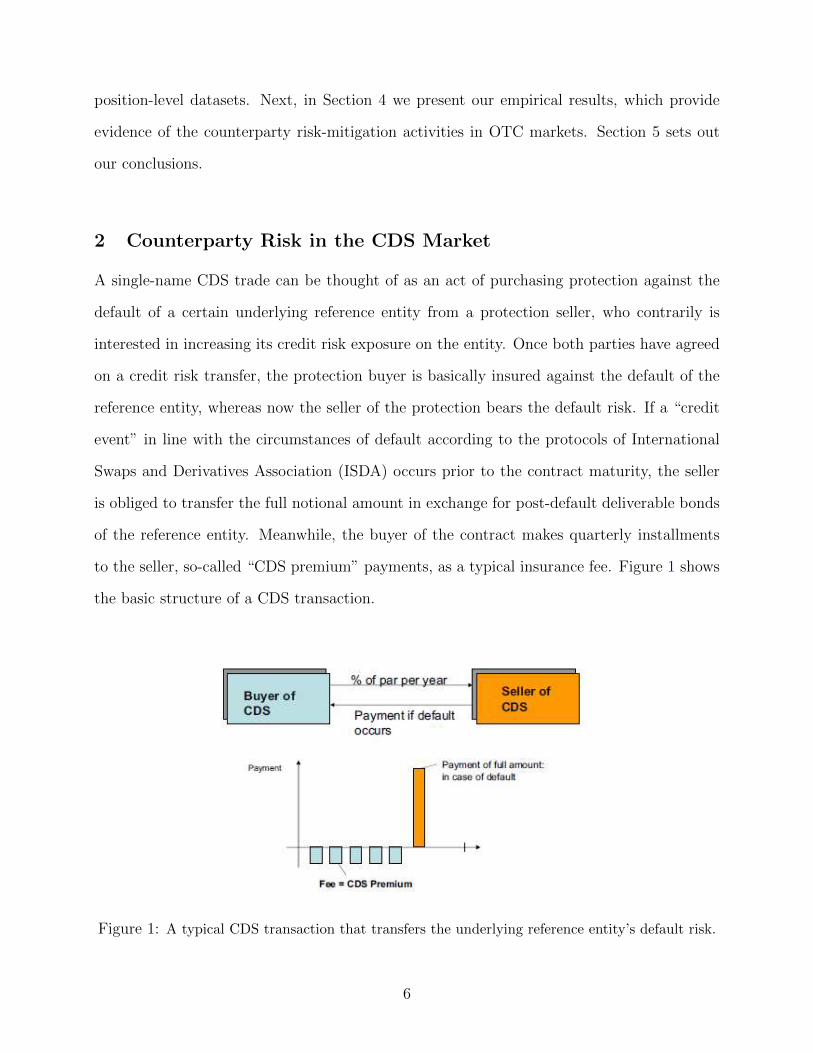
2 Counterparty Risk in the CDS Market
A single-name CDS trade can be thought of as an act of purchasing protection against the
default of a certain underlying reference entity from a protection seller, who contrarily is
interested in increasing its credit risk exposure on the entity. Once both parties have agreed
on a credit risk transfer, the protection buyer is basically insured against the default of the
reference entity, whereas now the seller of the protection bears the default risk. If a “credit
event” in line with the circumstances of default according to the protocols of International
Swaps and Derivatives Association (ISDA) occurs prior to the contract maturity, the seller
is obliged to transfer the full notional amount in exchange for post-default deliverable bonds
of the reference entity. Meanwhile, the buyer of the contract makes quarterly installments
to the seller, so-called “CDS premium” payments, as a typical insurance fee. Figure 1 shows
the basic structure of a CDS transaction.
Figure 1: A typical CDS transaction that transfers the underlying reference entity’s default risk.
6
The risk of the protection buyer not receiving the notional payment due to financial
constraints of the seller, even if the reference entity defaults, can be referred to as the “coun-
terparty risk” in CDS contracts. If the counterparty faces financial difficulties in parallel to
the reference entity, there is a danger that the buyer of the initial protection will not receive
his notional payment. Nevertheless, counterparty risk persists not just during a credit event
relating to the reference entity but at any time when the counterparty is in financial trouble,
since marking-to-market agreements and the need to post additional collateral can threaten
its position as a viable reverse side of the contract. In order to assess their expected loss
from the default of their counterparties, financial institutions calculate their credit valuation
adjustment or CVA, which is counterparty-specific and is a product of the probability of de-
fault, loss given default and expected net exposure for the counterparty. An increase in CVA
is deducted from the reported income of dealers, so that there is a general interest in keeping
the counterparty-specific credit exposure at lower levels. Moreover, this counterparty-specific
credit risk has also been introduced as a capital charge under the Basel III regulations (Basel
Committee on Banking Supervision (2011)).
How can the buyer protect himself against the possibility of deteriorating counterparty
credibility? Typically, ISDA master agreements and protocols provide a framework for a
healthy bilateral relationship between transacting parties. Most importantly, the high degree
of collateralization in the CDS market secures the system against any derailing. In this
paper, we specifically look at the counterparty risk-mitigation activity of buyers of protection
who might prefer to actively manage their risk above and beyond master agreements and
collateralization. Specifically, we investigate whether German banks that are active buyers
of CDS protection from one global counterparty undertake successive contracts and purchase
protection written on these global players. Providing significant evidence on mitigation of
counterparty risk even only on bilateral CDS exposures indicates that a much higher degree
of counterparty risk mitigation should be taking place if exposures from interest rate and FX
swaps were included.
7
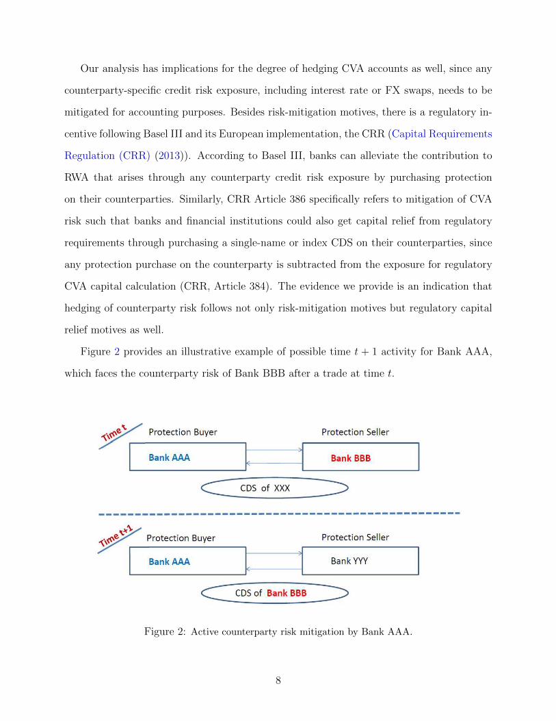
Our analysis has implications for the degree of hedging CVA accounts as well, since any
counterparty-specific credit risk exposure, including interest rate or FX swaps, needs to be
mitigated for accounting purposes. Besides risk-mitigation motives, there is a regulatory in-
centive following Basel III and its European implementation, the CRR (Capital Requirements
Regulation (CRR) (2013)). According to Basel III, banks can alleviate the contribution to
RWA that arises through any counterparty credit risk exposure by purchasing protection
on their counterparties. Similarly, CRR Article 386 specifically refers to mitigation of CVA
risk such that banks and financial institutions could also get capital relief from regulatory
requirements through purchasing a single-name or index CDS on their counterparties, since
any protection purchase on the counterparty is subtracted from the exposure for regulatory
CVA capital calculation (CRR, Article 384). The evidence we provide is an indication that
hedging of counterparty risk follows not only risk-mitigation motives but regulatory capital
relief motives as well.
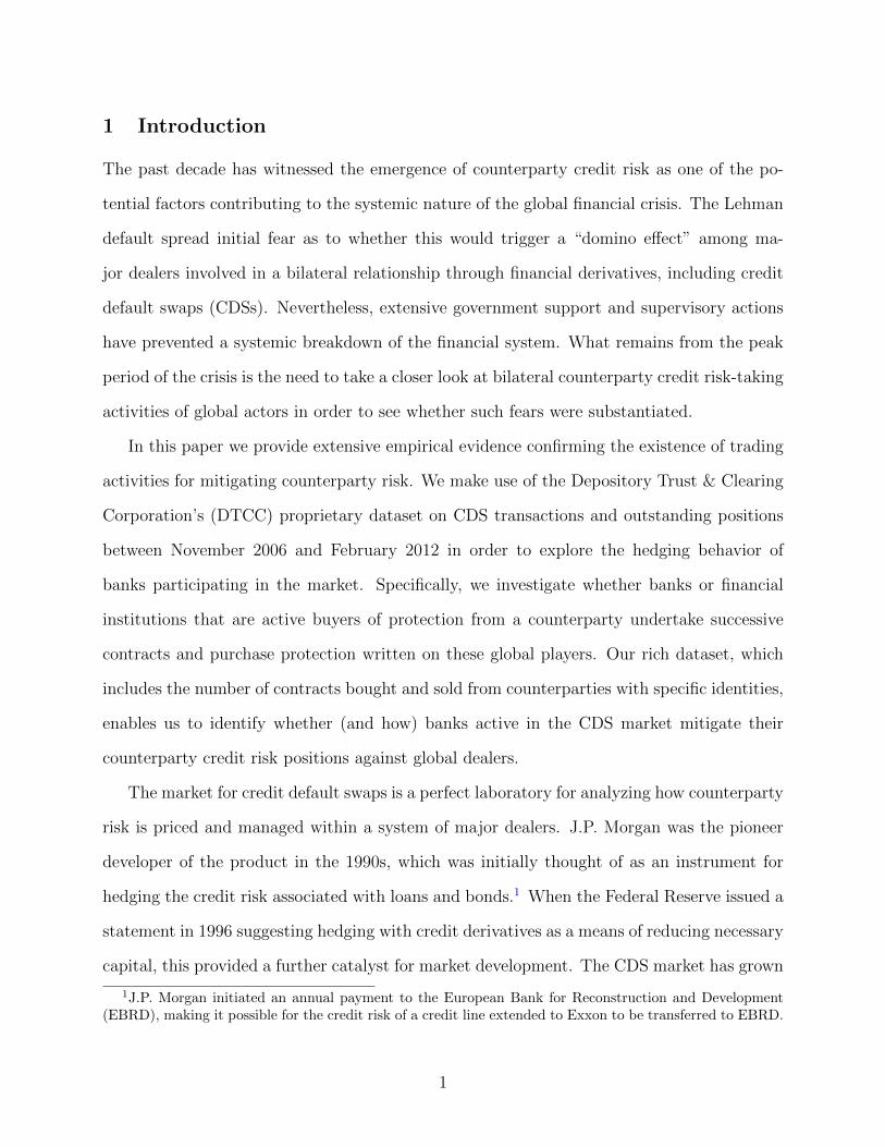
Figure 2 provides an illustrative example of possible time t + 1 activity for Bank AAA,
which faces the counterparty risk of Bank BBB after a trade at time t.
Figure 2: Active counterparty risk mitigation by Bank AAA.
8
Testing whether Bank AAA actively takes action to mitigate counterparty risk of Bank
BBB at t + 1 is central to our analysis. Such an investigation could not have been made in
the past, as bilateral transaction data on CDS has only recently become available through
trade repositories. Our proprietary DTCC data on CDS transactions is presented in the next
section.
3 Bank-Specific Credit Default Swap Data from the DTCC
3.1 Transaction-Level Dataset
There is a vast amount of literature based on daily CDS composite prices or quotes that look
at an aggregated set of information on credit risk. Since the trading of credit default swaps
was primarily achieved on the over-the-counter market prior to the introduction of central
counterparties, empirical research in financial literature was limited to depending on this
type of composite data. The recent formation of trade repositories has made it possible to
analyze bank activities not only for regulation purposes, but also in the world of academia.
The DTCC pioneered in the trade repository market with its Trade Information Ware-
house (TIW), which actively started capturing transactions in 2008. In parallel, all earlier
trades that are still open have been frontloaded, which means that they were transferred to
TIW after their inception. The DTCC thereby estimates its coverage for all globally traded
single-name CDS to stand at 95% and 99%, respectively, in terms of number of contracts and
notional amounts (Gunduz et al. (2017)). A summary of the growing academic literature
using TIW data of the DTCC can be found in Acharya, Gunduz, and Johnson (2017).
The DTCC provided access to all CDS transactions of German banks and financial insti-
tutions, as well as the positions associated with these transactions. Our baseline transaction-
level dataset encompasses all new trades from November 2006 to February 2012. These are
the actual new CDS transactions bought (sold) by German financial institutions from (to)
any global counterparty, as well as any CDS contracts bought or sold on these counterparties
9
where they are a reference entity. The DTCC tags financial institutions in the CDS market
as “dealer” or “buyside”. Prior research shows that counterparties tagged as “dealers” by the
DTCC are either on the buy (85%) or the sell side (89%) of a CDS trade. The full universe
of TIW positions confirms this high concentration (89% for being on the buy or sell side)
with publicly available data (Gunduz et al. (2017)). Since our sample includes all the trading
activity with these global dealers, it is highly representative of the global CDS trading which
is known to have dealer dominance. Moreover, focusing on dealers as the counterparties
for German financial institutions has the advantage of avoiding the usage of transactions by
counterparties that rarely trade and/or are rarely traded as a reference entity.
A group of 25 German banks and financial institutions reside in our sample, the aim being
to look at their counterparty risk-mitigation behavior. Their names could not be explicitly
mentioned due to confidentiality reasons. On the other hand, Table 1 consists of the 21
counterparties that DTCC tags as global dealers.3,4
All of the new CDS protection bought from these dealers, as well as all of the new CDS
bought on these dealers as reference entities, will be investigated concurrently in this study.
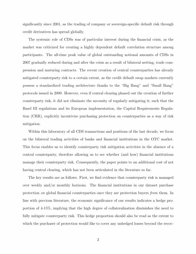
Figures 3 and 4 shed light on the time series development of the counterparty risk-taking
and mitigation activities of German banks on global dealers. In Figure 3, it can be seen that
purchasing protection from dealers reached an all-time high of 600 new contracts during the
week of September 15-19, 2008, at the peak of the subprime mortgage crisis when Lehman
Brothers defaulted, and then partly slowed down towards the end of our sample period. We
term this type of transactions as “SEL”, where the global counterparty acts as the seller of
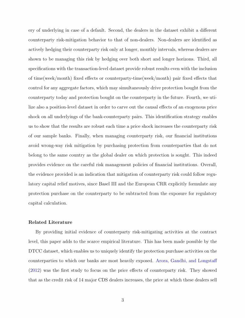
the contract. Similarly, Figure 4 shows that purchasing protection on dealers reached a value
of 235 new contracts during the same week in which Lehman Brothers defaulted, but as the
3It should be noted that these include the G14 dealers: Bank of America-Merrill Lynch, Barclays Capital,BNP Paribas, Citi, Credit Suisse, Deutsche Bank, Goldman Sachs, HSBC, JP Morgan, Morgan Stanley, RBS,Societe Generale, UBS, and Wells Fargo Bank. Peltonen, Scheicher, and Vuillemey (2014) provide empiricalevidence that the CDS market is centered around G14 dealers.
4It should be noted that Deutsche Bank AG and Commerzbank AG are present in both samples. Forour purposes, they will serve as German banks when their counterparty risk-taking behavior on dealers isbeing investigated, and as dealers against other German banks and financial institutions whenever they actas counterparties for the remaining 23 institutions included in our German sample.
10
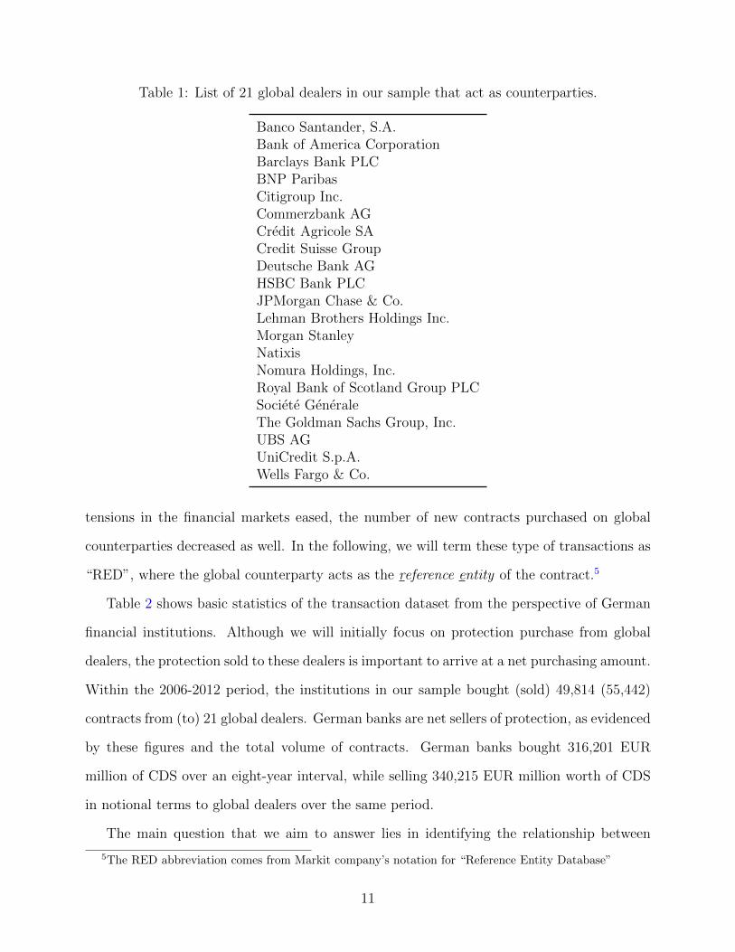
Table 1: List of 21 global dealers in our sample that act as counterparties.
Banco Santander, S.A.Bank of America CorporationBarclays Bank PLCBNP ParibasCitigroup Inc.Commerzbank AGCredit Agricole SACredit Suisse GroupDeutsche Bank AGHSBC Bank PLCJPMorgan Chase & Co.Lehman Brothers Holdings Inc.Morgan StanleyNatixisNomura Holdings, Inc.Royal Bank of Scotland Group PLCSociete GeneraleThe Goldman Sachs Group, Inc.UBS AGUniCredit S.p.A.Wells Fargo & Co.
tensions in the financial markets eased, the number of new contracts purchased on global
counterparties decreased as well. In the following, we will term these type of transactions as
“RED”, where the global counterparty acts as the reference entity of the contract.5
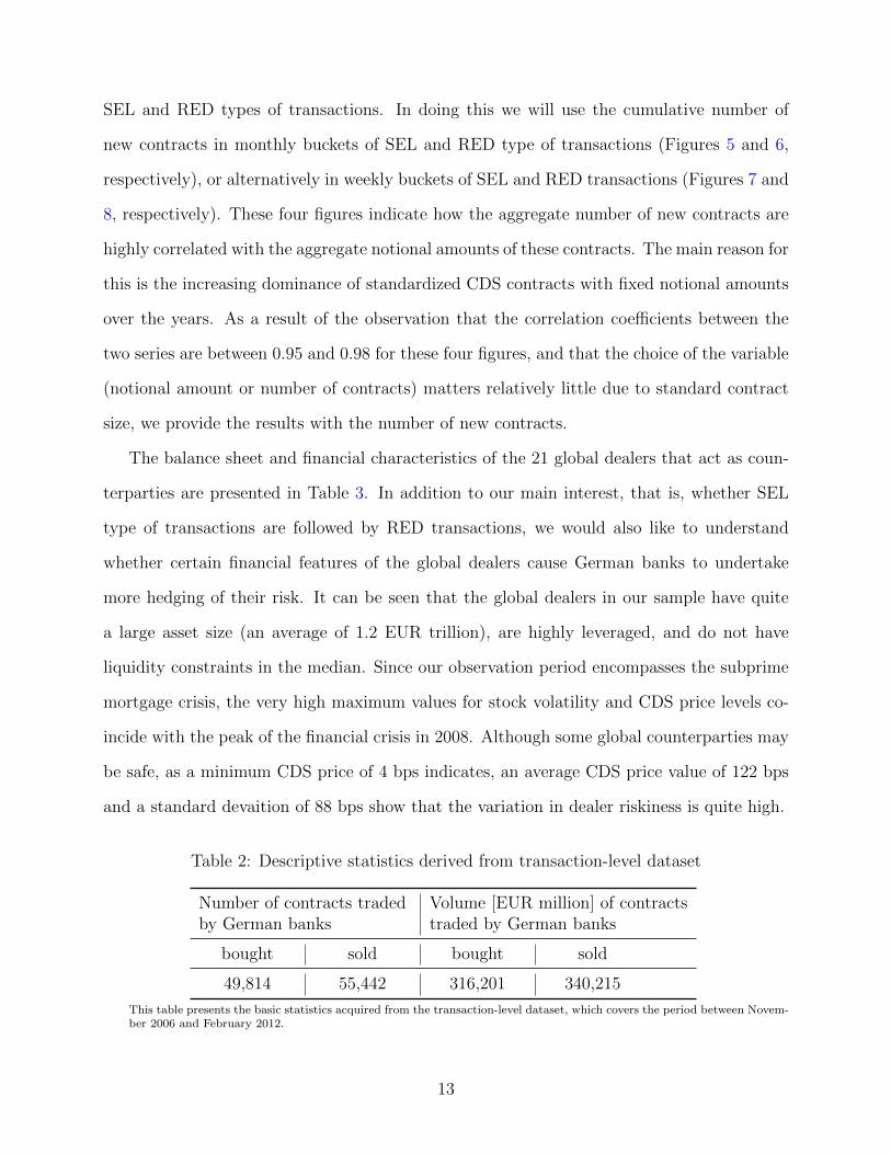
Table 2 shows basic statistics of the transaction dataset from the perspective of German
financial institutions. Although we will initially focus on protection purchase from global
dealers, the protection sold to these dealers is important to arrive at a net purchasing amount.
Within the 2006-2012 period, the institutions in our sample bought (sold) 49,814 (55,442)
contracts from (to) 21 global dealers. German banks are net sellers of protection, as evidenced
by these figures and the total volume of contracts. German banks bought 316,201 EUR
million of CDS over an eight-year interval, while selling 340,215 EUR million worth of CDS
in notional terms to global dealers over the same period.
The main question that we aim to answer lies in identifying the relationship between
5The RED abbreviation comes from Markit company’s notation for “Reference Entity Database”
11
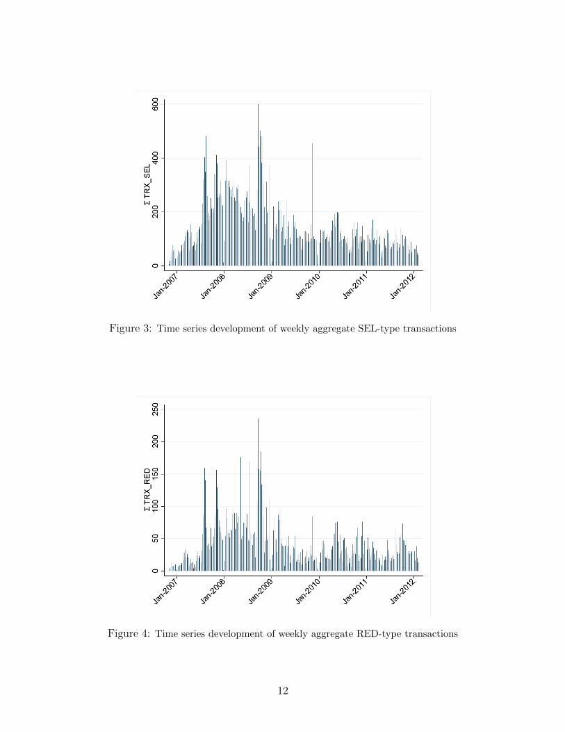
Figure 3: Time series development of weekly aggregate SEL-type transactions
Figure 4: Time series development of weekly aggregate RED-type transactions
12
SEL and RED types of transactions. In doing this we will use the cumulative number of
new contracts in monthly buckets of SEL and RED type of transactions (Figures 5 and 6,
respectively), or alternatively in weekly buckets of SEL and RED transactions (Figures 7 and
8, respectively). These four figures indicate how the aggregate number of new contracts are
highly correlated with the aggregate notional amounts of these contracts. The main reason for
this is the increasing dominance of standardized CDS contracts with fixed notional amounts
over the years. As a result of the observation that the correlation coefficients between the
two series are between 0.95 and 0.98 for these four figures, and that the choice of the variable
(notional amount or number of contracts) matters relatively little due to standard contract
size, we provide the results with the number of new contracts.
The balance sheet and financial characteristics of the 21 global dealers that act as coun-
terparties are presented in Table 3. In addition to our main interest, that is, whether SEL
type of transactions are followed by RED transactions, we would also like to understand
whether certain financial features of the global dealers cause German banks to undertake
more hedging of their risk. It can be seen that the global dealers in our sample have quite
a large asset size (an average of 1.2 EUR trillion), are highly leveraged, and do not have
liquidity constraints in the median. Since our observation period encompasses the subprime
mortgage crisis, the very high maximum values for stock volatility and CDS price levels co-
incide with the peak of the financial crisis in 2008. Although some global counterparties may
be safe, as a minimum CDS price of 4 bps indicates, an average CDS price value of 122 bps
and a standard devaition of 88 bps show that the variation in dealer riskiness is quite high.
Table 2: Descriptive statistics derived from transaction-level dataset
Number of contracts traded Volume [EUR million] of contractsby German banks traded by German banks
bought sold bought sold
49,814 55,442 316,201 340,215
This table presents the basic statistics acquired from the transaction-level dataset, which covers the period between Novem-ber 2006 and February 2012.
13
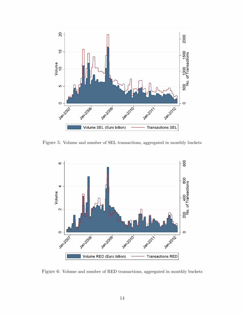
Figure 5: Volume and number of SEL transactions, aggregated in monthly buckets
Figure 6: Volume and number of RED transactions, aggregated in monthly buckets
14

Figure 7: Volume and number of SEL transactions, aggregated in weekly buckets
Figure 8: Volume and number of RED transactions, aggregated in weekly buckets
15

Table 3: Summary statistics for financial variables of 21 global dealers
VARIABLES N Mean S.D. Min 10th 50th 90th Max
Total Assets (EUR billion) 5,318 1,235.20 556.75 156.35 548.87 1,162.32 1,957.75 3,027.84Capital Structure 5,318 0.95 0.02 0.89 0.91 0.95 0.98 0.99Current Ratio 5,318 1.17 0.56 0.26 0.60 1.09 1.80 4.77Stock Return (%) 5,318 -0.15 2.10 -42.98 -1.87 -0.11 1.60 16.75Stock Volatility 5,318 1.48 2.03 0.01 0.17 0.85 3.42 25.24CDS Volatility (bps) 5,318 7.08 13.40 0.01 0.90 4.30 14.43 411.00CDS Price (bps) 5,318 122.07 88.18 4.28 29.66 106.30 217.36 1,182.35
This table contains summary statistics for financial variables of 21 global dealers as counterparties. Listed in the table areweekly summary statistics (number of observations, mean, standard deviation, minimum, 10th, 50th and 90th percentiles, andmaximum) in the sample period between November 2006 and February 2012. Quarterly values for Total Assets, Captial Structureand Current Ratio are repeated in this table as weekly observations, since the following regression analyses makes use of weeklydata points. Total Assets of the 21 global counterparties are in billion euros. Capital Structure is defined as total liabilitiesdivided by total assets. Current Ratio is defined as one-year liquid assets (marketable securities, other short-term investments,cash and cash-near items) over one-year liabilities (short-term borrowing, securities sold as repos, short-term liabilities andcustomer accounts). Stock Return and Stock Volatility are defined as geometric average of trading week stock return andthe standard deviation of trading week stock returns of the global counterparty, respectively. CDS Volatility is the standarddeviation of CDS price levels of the trading week, whereas CDS price is the arithmetic average CDS spread level of the sameweek. Data sources are Bankscope, Bloomberg and Markit.
3.2 Position-Level Dataset
The position-level dataset from DTCC provides an alternative answer to the research ques-
tion. In contrast to the “flow” information provided by the transaction-level dataset, the
position-level dataset contains “stock” information. These snapshots encompass the Jan-
uary 2008 to February 2012 weekly CDS positions of all the above-mentioned 25 financial
institutions. Although the DTCC started building its database in 2008, the position dataset
contains all the prior transactions that are frontloaded as well. Moreover, this dataset serves
as a perfect tool for testing the robustness of the transaction-level results, since all other types
of CDS transactions, such as assignments, amendments, and terminations are now embedded
in the information in the number of open contracts. Moreover, the maturity of each new
transaction is automatically accounted for when all open trades in the position level dataset
are considered.
Table 4 Panel A provides basic descriptive statistics on the weekly average number of
open contracts of banks and institutions in our sample on dealer banks as the underlying,
and on dealer banks as the counterparty. Although the confidential nature of the data does
16
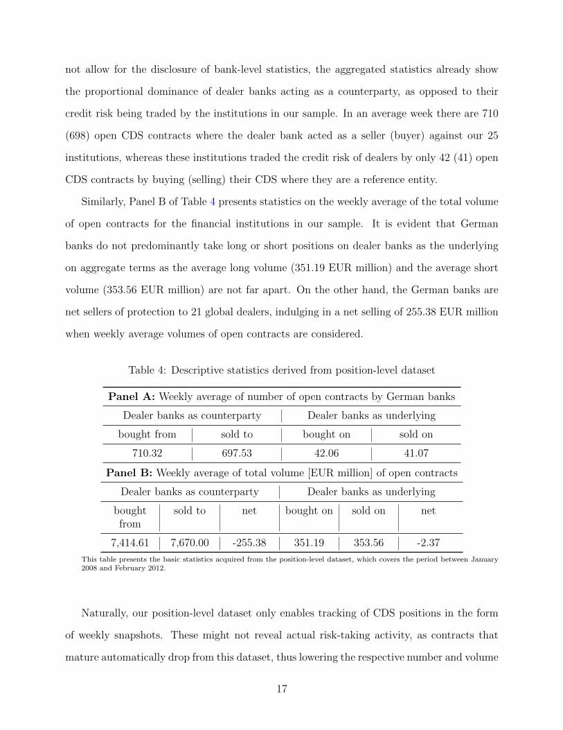
not allow for the disclosure of bank-level statistics, the aggregated statistics already show
the proportional dominance of dealer banks acting as a counterparty, as opposed to their
credit risk being traded by the institutions in our sample. In an average week there are 710
(698) open CDS contracts where the dealer bank acted as a seller (buyer) against our 25
institutions, whereas these institutions traded the credit risk of dealers by only 42 (41) open
CDS contracts by buying (selling) their CDS where they are a reference entity.
Similarly, Panel B of Table 4 presents statistics on the weekly average of the total volume
of open contracts for the financial institutions in our sample. It is evident that German
banks do not predominantly take long or short positions on dealer banks as the underlying
on aggregate terms as the average long volume (351.19 EUR million) and the average short
volume (353.56 EUR million) are not far apart. On the other hand, the German banks are
net sellers of protection to 21 global dealers, indulging in a net selling of 255.38 EUR million
when weekly average volumes of open contracts are considered.
Table 4: Descriptive statistics derived from position-level dataset
Panel A: Weekly average of number of open contracts by German banks
Dealer banks as counterparty Dealer banks as underlying
bought from sold to bought on sold on
710.32 697.53 42.06 41.07
Panel B: Weekly average of total volume [EUR million] of open contracts
Dealer banks as counterparty Dealer banks as underlying
boughtfrom
sold to net bought on sold on net
7,414.61 7,670.00 -255.38 351.19 353.56 -2.37
This table presents the basic statistics acquired from the position-level dataset, which covers the period between January2008 and February 2012.
Naturally, our position-level dataset only enables tracking of CDS positions in the form
of weekly snapshots. These might not reveal actual risk-taking activity, as contracts that
mature automatically drop from this dataset, thus lowering the respective number and volume
17
of contracts. Although it may be argued that maturing bought contracts would, on average,
be equivalent to maturing sold contracts, the position-level dataset will be an ideal tool to be
utilized in Section 4.3 for a better identification through price shocks to the individual position
with the counterparty. All in all, both datasets will be important sources for understanding
risk-taking activities by the financial institutions in our sample. The findings from the two
datasets would complement each other in this manner.
4 Empirical Analysis
4.1 Evidence of Risk Mitigation from Baseline Transaction Datasets
We are initially interested in the trading activity in rolling weeks or months. Our selection
of alternative time intervals overlaps with the margin period at risk for CVA calculation.
The so-called “cure period” is the time that elapses between when the counterparty ceases
to post collateral and the financial institution is able to hedge this uncovered risk. This can
be regarded as the actual grace period in which no collateral is posted and the institution
is exposed to naked counterparty risk, and therefore the institution takes action in order to
cover remaining exposure. In practice, a cure period of 10 to 25 business days is typical. It
is initially hypothesized that the banks and financial institutions in our sample undertake
trading activity in the form of CDS purchasing on a global counterparty as an underlying
entity following a month of CDS purchases from that same global counterparty. By collecting
the flow information in monthly buckets, any successive hedging activity can be identified at
rolling intervals.6 The first specification we examine is as follows:
4∑k=1
REDi,j,t+k = a0 + a1
3∑k=0
SELi,j,t−k + a2Xj,t + FE + εi,j,t (1)
where SEL is the cumulative number of contracts bought by the German bank i when the
counterparty j acts as a seller between (and including) weeks t = 0 and t = −3, and RED is
6In this way, the rolling methodology could also capture any chain of consecutive hedging on each nextcounterparty.
18
the cumulative number of contracts bought by the German bank i where the counterparty
j is a reference entity between (and including) weeks t=4 and t=1. We expect a positive
coefficient for a1 if the banks i aim at hedging their risk on counterparties j on monthly
rolling horizons. Vector X represents the counterparty-specific variables such as total assets,
capital structure, current ratio (of their last quarter), geometric average stock return and
volatility (in their last month), and average CDS price and volatility (in their last month).
All specifications are alternatively tested using bank fixed effects, counterparty fixed effects
and bank-counterparty pair fixed effects. In this way, we are able to address any idiosyncratic
effects arising from our banks and their counterparties. In addition, all specifications include
time(month) fixed effects or counterparty-time(month) pair fixed effects in order to control for
any aggregate factors that may simultaneously drive protection bought from the counterparty
today and protection bought on the counterparty in the future. All errors are clustered at
the bank level. As a robustness check, we also cluster the errors at the bank-counterparty
pair level as an alternative.
Table 5 presents the results of the baseline dataset of monthly cumulative rolling trans-
actions. The main variable of interest, the monthly lagged cumulative new transactions of
protection bought from the counterparty is positive, and always significant in explaining the
following month’s cumulative new protections bought on the counterparty. Even the highly
constraining bank-counterparty pair fixed effect (with more than 200 dummies) in specifica-
tions (3),(4),(8) and (9) does not diminish the significance of the main variable of interest.
It is important to underline that the significance is also persistent, regardless of whether the
errors are clustered at bank level (with 24-25 clusters) or bank-counterparty pair level (with
more than 200 clusters).7 Finally, the a1 parameter, which is significantly positive even in
specification (5), ensures that accounting for counterparty-specific time-variant effects does
not alter the results, and addresses any endogeneity concerns by showing that the results are
7When there is a small number of clusters, or when there are very unbalanced cluster sizes, the inferenceusing the cluster-robust estimator may be biased. As long as bank-level clustering is undertaken, our dealerbanks have a higher number of observations than non-dealer banks, which makes it necessary to check therobustness of the results to bank-counterparty pair clustering.
19

Table 5: Mitigation of counterparty risk – Monthly rolling intervals of cumulative new transactions
(1) (2) (3) (4) (5) (6) (7) (8) (9)VARIABLES Σ TRX RED Σ TRX RED Σ TRX RED Σ TRX RED Σ TRX RED Σ TRX RED Σ TRX RED Σ TRX RED Σ TRX RED
L4.Σ TRX SEL 0.0954*** 0.147*** 0.0491*** 0.0491** 0.155*** 0.0796*** 0.146*** 0.0364*** 0.0364**(0.0113) (0.0114) (0.00674) (0.0205) (0.00842) (0.00827) (0.0131) (0.0103) (0.0152)
TOT ASSETS (QLAG) (e-10) 4.85 9.41 -0.477 -0.477(3.26) (8.02) (4.25) (9.06)
CAP STRUCTURE (QLAG) -15.63 56.72 110.0* 110.0**(12.58) (42.83) (62.01) (46.31)
CURRENT RATIO (QLAG) 1.001 -0.304* -0.429*** -0.429(0.712) (0.154) (0.137) (0.292)
L4.STOCK RETURN -49.22 -38.44 -46.45* -46.45***(31.12) (25.32) (26.20) (14.82)
L4.STOCK VOLATILITY 0.172 -0.337** 0.0343 0.0343(0.142) (0.147) (0.0656) (0.322)
L4.CDS VOLATILITY 0.0241 0.0132 0.0177 0.0177(0.0361) (0.0217) (0.0236) (0.0463)
L4.CDS PRICE (e-4) 160.0* 75.7 103.0 103.0***(91.9) (45.3) (61.5) (34.9)
Constant -5.868*** 3.826** -11.16*** -11.16*** 1.086 6.000 -51.89 -117.4* -117.4***(0.261) (1.549) (0.460) (0.832) (0.667) (10.51) (43.24) (60.71) (44.47)
Observations 12057 12057 12057 12057 12057 9486 9486 9486 9486
Adjusted R2 0.341 0.355 0.142 0.142 0.453 0.380 0.347 0.176 0.176
Bank FE/# YES/25 NO NO NO NO YES/24 NO NO NOCparty FE/# NO YES/21 NO NO NO NO YES/20 NO NOMonth FE/# YES/65 YES/65 YES/65 YES/65 NO YES/65 YES/65 YES/65 YES/65Bank-Cparty FE/# NO NO YES/219 YES/219 NO NO NO YES/208 YES/208Cparty-Month FE/# NO NO NO NO YES/1172 NO NO NO NOError Clustering Bank Bank Bank Bank-Cparty Bank Bank Bank Bank Bank-Cparty
This table presents the coefficients from fixed-effect regressions with bank, counterparty, bank-counterparty pair, month and counterparty-month pair fixed effects. Columns(1) and (6) present the coefficients for linear regressions with fixed effects on the German banks (bank FE) and time (month FE), whereas the coefficients presented in columns(2) and (7) are based on linear regressions with global dealer bank (counterparty FE) and time (month) fixed effects. Regression results presented in columns (3), (4), (8) and(9) use bank-counterparty pair in addition to month fixed effects. Column (5) presents the coefficient for linear regression with counterparty-month pair fixed effect. The timehorizon is from November 2006 to February 2012 and the difference between two units of time is one week. Σ TRX RED is the number of new transactions within the followingfour weeks where the German bank serves as the buyer and the global counterparty as the underlying. Σ TRX SEL contains the number of new transactions entered within thisweek and the three previous weeks where the German bank serves as the buyer and the global counterparty as the seller. The variables TOT ASSETS, CAP STRUCTURE,and CURRENT RATIO contain the total assets, the capital structure and the current ratio of the counterparty lagged by one quarter. The variables STOCK RETURN andSTOCK VOLATILITY contain the geometric average stock return and the standard deviation of the weekly stock return of the counterparty in the past month, respectively.CDS PRICE contains the CDS spread level of the past month, whereas CDS VOLATILITY is the standard deviation of the CDS price within the last month. Robust standarderrors clustered at either bank or bank-counterparty pair level are in parentheses. The symbols ∗ ∗ ∗, ∗∗, and ∗ indicate significance levels of 1%, 5% and 10%, respectively.
20
not driven by counterparty-specific or aggregate factors in certain months.8
Moreover, what we may refer to as the “hedge proportion” is at economically reasonable
levels. For each contract bought from counterparties, 4− 15% of contracts are bought on the
counterparties. These values provide a good estimate for the counterparty risk-mitigation
activity beyond any usage of collateral and any expected retained amount due to recovery in
case of a default. The high extent of collateralization in the CDS market is documented in
Arora et al. (2012), such that collateral agreements were included in 74% of CDS contracts
that were executed in 2008. The economic significance of the hedge proportion can be
interpreted in terms of the expected recovery from the underlying and the non-collateralized
portion for an average trade. A standard assumption for the average recovery of a corporate
bond would be at the 40% level. Hence, the buyer of the CDS would receive 60% of the
notional amount as a payoff from the seller, in case of a default of the reference entity. With
a back-of-the-envelope calculation, if the buyer of the CDS has received collateral for 74%
of the contracts with the seller, counterparty risk could be further hedged for a remaining
15.6% of the contracts, which is a value close to the maximum hedge proportion revealed by
our coefficients.
Given that the transaction-level data enables a fine picture of risk-taking activity, one can
consider a weekly cumulation of buckets with a view to identify short-term trading activities.
REDi,j,t+1 = a0 + a1SELi,j,t + a2Xj,t + FE + εi,j,t (2)
The specification in Equation (2) would collect all transactions on weekly rolling horizons.
All other variables are identical to the first specification. The results in Table 6 mirror the
findings in Table 5 such that new transactions of protections bought from the counterparty
positively explain the following week’s new protections bought on the counterparty. In Table
8An alternative specification that was looked at used the net (bought - sold) number of new transactionstraded with/on the counterparty. The main variable of interest was still significantly positive, and themagnitude was naturally lower. The results are therefore robust when protections sold to/on the counterpartyare considered.
21
6, all nine specifications (with an exception of specification (5)) include time(week) fixed
effects in order to control for any aggregate factors that may simultaneously drive protection
bought from the counterparty today and protection bought on the counterparty in the follow-
ing weeks. Specification (5) alternatively provides the results with counterparty-week fixed
effects. The a1 parameter, which is robustly positive in all nine cases, once again confirms
that accounting for time-variant effects does not alter the results, and that the results are
not driven by counterparty-specific or aggregate shocks in certain weeks.
The regressions with the weekly baseline dataset deliver further interesting observations.
The full specifications ((6)-(9)) reveal that protection purchase activity is prevalent on coun-
terparties that have a larger asset size. While the evidence on the current ratio and leverage
is not conclusive, a decrease in the past week’s stock returns and a higher stock return volatil-
ity leads to increased protection purchase on the counterparty. Most importantly, there is
strong evidence that the CDS of riskier counterparties that have a higher CDS price level
are purchased more. These intuitive results contribute to the analysis of counterparty risk
mitigation.
An interesting extension to Table 6 is to include interacting variables with the protection
bought from the counterparty. These interaction terms would show which attributes of the
counterparty complement the explanation of the hedging behavior of our financial institu-
tions. Table 7 provides this analysis based on bank, counterparty, and bank-counterparty
pair fixed effects, in addition to the time (week) fixed effects in each specification. The inter-
acting variables indicate that lower past stock returns and increased stock volatility of the
counterparty encourage the banks to purchase more CDS protection on these counterparties,
possibly as insurance during turbulent times that the counterparty might be facing. The
CDS price volatility of the counterparty has a similar effect on protection purchasing on
these counterparties. All these variables indicate a higher degree of risk mitigation by the
financial institutions.
22
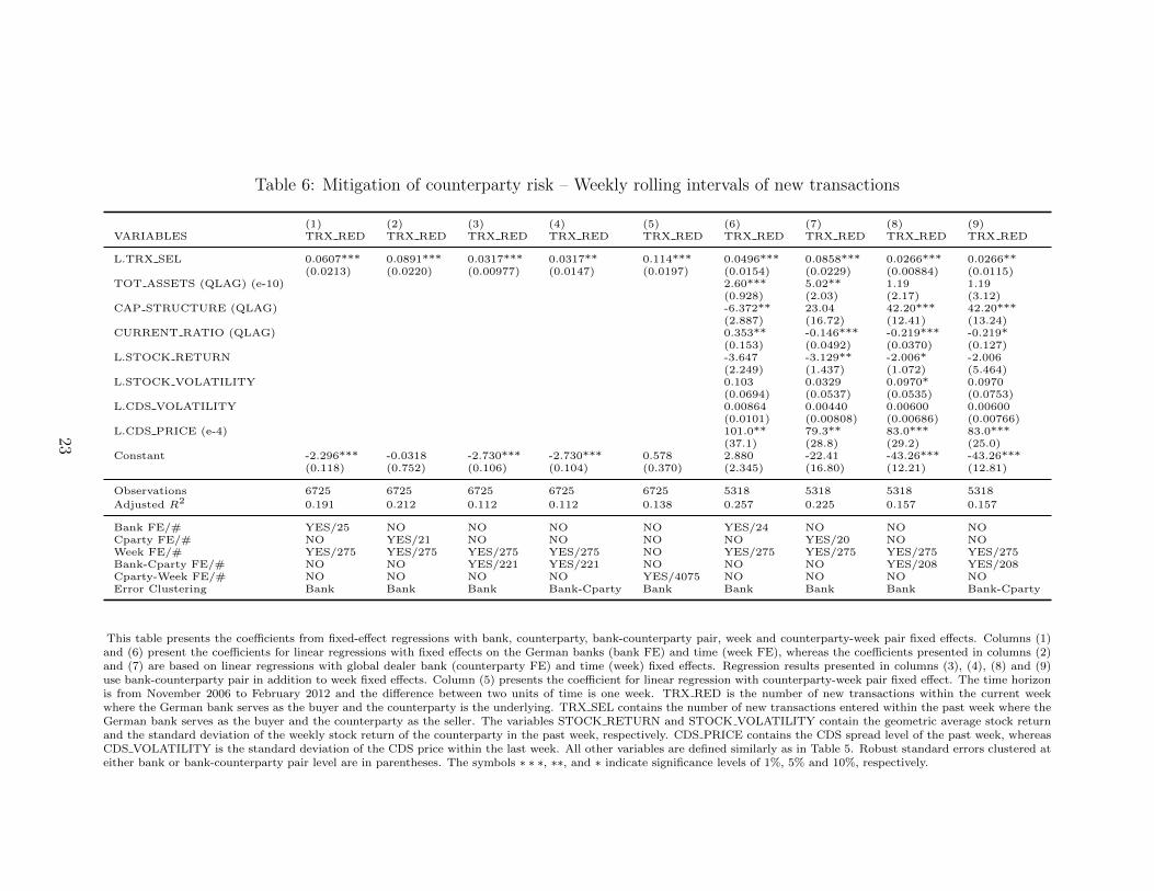
Table 6: Mitigation of counterparty risk – Weekly rolling intervals of new transactions
(1) (2) (3) (4) (5) (6) (7) (8) (9)VARIABLES TRX RED TRX RED TRX RED TRX RED TRX RED TRX RED TRX RED TRX RED TRX RED
L.TRX SEL 0.0607*** 0.0891*** 0.0317*** 0.0317** 0.114*** 0.0496*** 0.0858*** 0.0266*** 0.0266**(0.0213) (0.0220) (0.00977) (0.0147) (0.0197) (0.0154) (0.0229) (0.00884) (0.0115)
TOT ASSETS (QLAG) (e-10) 2.60*** 5.02** 1.19 1.19(0.928) (2.03) (2.17) (3.12)
CAP STRUCTURE (QLAG) -6.372** 23.04 42.20*** 42.20***(2.887) (16.72) (12.41) (13.24)
CURRENT RATIO (QLAG) 0.353** -0.146*** -0.219*** -0.219*(0.153) (0.0492) (0.0370) (0.127)
L.STOCK RETURN -3.647 -3.129** -2.006* -2.006(2.249) (1.437) (1.072) (5.464)
L.STOCK VOLATILITY 0.103 0.0329 0.0970* 0.0970(0.0694) (0.0537) (0.0535) (0.0753)
L.CDS VOLATILITY 0.00864 0.00440 0.00600 0.00600(0.0101) (0.00808) (0.00686) (0.00766)
L.CDS PRICE (e-4) 101.0** 79.3** 83.0*** 83.0***(37.1) (28.8) (29.2) (25.0)
Constant -2.296*** -0.0318 -2.730*** -2.730*** 0.578 2.880 -22.41 -43.26*** -43.26***(0.118) (0.752) (0.106) (0.104) (0.370) (2.345) (16.80) (12.21) (12.81)
Observations 6725 6725 6725 6725 6725 5318 5318 5318 5318
Adjusted R2 0.191 0.212 0.112 0.112 0.138 0.257 0.225 0.157 0.157
Bank FE/# YES/25 NO NO NO NO YES/24 NO NO NOCparty FE/# NO YES/21 NO NO NO NO YES/20 NO NOWeek FE/# YES/275 YES/275 YES/275 YES/275 NO YES/275 YES/275 YES/275 YES/275Bank-Cparty FE/# NO NO YES/221 YES/221 NO NO NO YES/208 YES/208Cparty-Week FE/# NO NO NO NO YES/4075 NO NO NO NOError Clustering Bank Bank Bank Bank-Cparty Bank Bank Bank Bank Bank-Cparty
This table presents the coefficients from fixed-effect regressions with bank, counterparty, bank-counterparty pair, week and counterparty-week pair fixed effects. Columns (1)and (6) present the coefficients for linear regressions with fixed effects on the German banks (bank FE) and time (week FE), whereas the coefficients presented in columns (2)and (7) are based on linear regressions with global dealer bank (counterparty FE) and time (week) fixed effects. Regression results presented in columns (3), (4), (8) and (9)use bank-counterparty pair in addition to week fixed effects. Column (5) presents the coefficient for linear regression with counterparty-week pair fixed effect. The time horizonis from November 2006 to February 2012 and the difference between two units of time is one week. TRX RED is the number of new transactions within the current weekwhere the German bank serves as the buyer and the counterparty is the underlying. TRX SEL contains the number of new transactions entered within the past week where theGerman bank serves as the buyer and the counterparty as the seller. The variables STOCK RETURN and STOCK VOLATILITY contain the geometric average stock returnand the standard deviation of the weekly stock return of the counterparty in the past week, respectively. CDS PRICE contains the CDS spread level of the past week, whereasCDS VOLATILITY is the standard deviation of the CDS price within the last week. All other variables are defined similarly as in Table 5. Robust standard errors clustered ateither bank or bank-counterparty pair level are in parentheses. The symbols ∗ ∗ ∗, ∗∗, and ∗ indicate significance levels of 1%, 5% and 10%, respectively.
23
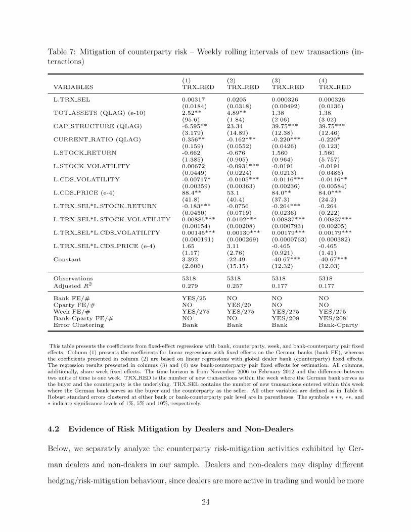
Table 7: Mitigation of counterparty risk – Weekly rolling intervals of new transactions (in-teractions)
(1) (2) (3) (4)VARIABLES TRX RED TRX RED TRX RED TRX RED
L.TRX SEL 0.00317 0.0205 0.000326 0.000326(0.0184) (0.0318) (0.00492) (0.0136)
TOT ASSETS (QLAG) (e-10) 2.52** 4.89** 1.38 1.38(95.6) (1.84) (2.06) (3.02)
CAP STRUCTURE (QLAG) -6.595** 23.34 39.75*** 39.75***(3.179) (14.89) (12.38) (12.46)
CURRENT RATIO (QLAG) 0.356** -0.162*** -0.220*** -0.220*(0.159) (0.0552) (0.0426) (0.123)
L.STOCK RETURN -0.662 -0.676 1.560 1.560(1.385) (0.905) (0.964) (5.757)
L.STOCK VOLATILITY 0.00672 -0.0931*** -0.0191 -0.0191(0.0449) (0.0224) (0.0213) (0.0486)
L.CDS VOLATILITY -0.00717* -0.0105*** -0.0116*** -0.0116**(0.00359) (0.00363) (0.00236) (0.00584)
L.CDS PRICE (e-4) 88.4** 53.1 84.0** 84.0***(41.8) (40.4) (37.3) (24.2)
L.TRX SEL*L.STOCK RETURN -0.183*** -0.0756 -0.264*** -0.264(0.0450) (0.0719) (0.0236) (0.222)
L.TRX SEL*L.STOCK VOLATILITY 0.00885*** 0.0102*** 0.00837*** 0.00837***(0.00154) (0.00208) (0.000793) (0.00205)
L.TRX SEL*L.CDS VOLATILITY 0.00145*** 0.00130*** 0.00179*** 0.00179***(0.000191) (0.000269) (0.0000763) (0.000382)
L.TRX SEL*L.CDS PRICE (e-4) 1.65 3.11 -0.465 -0.465(1.17) (2.76) (0.921) (1.41)
Constant 3.392 -22.49 -40.67*** -40.67***(2.606) (15.15) (12.32) (12.03)
Observations 5318 5318 5318 5318
Adjusted R2 0.279 0.257 0.177 0.177
Bank FE/# YES/25 NO NO NOCparty FE/# NO YES/20 NO NOWeek FE/# YES/275 YES/275 YES/275 YES/275Bank-Cparty FE/# NO NO YES/208 YES/208Error Clustering Bank Bank Bank Bank-Cparty
This table presents the coefficients from fixed-effect regressions with bank, counterparty, week, and bank-counterparty pair fixedeffects. Column (1) presents the coefficients for linear regressions with fixed effects on the German banks (bank FE), whereasthe coefficients presented in column (2) are based on linear regressions with global dealer bank (counterparty) fixed effects.The regression results presented in columns (3) and (4) use bank-counterparty pair fixed effects for estimation. All columns,additionally, share week fixed effects. The time horizon is from November 2006 to February 2012 and the difference betweentwo units of time is one week. TRX RED is the number of new transactions within the week where the German bank serves asthe buyer and the counterparty is the underlying. TRX SEL contains the number of new transactions entered within this weekwhere the German bank serves as the buyer and the counterparty as the seller. All other variables are defined as in Table 6.Robust standard errors clustered at either bank or bank-counterparty pair level are in parentheses. The symbols ∗ ∗ ∗, ∗∗, and∗ indicate significance levels of 1%, 5% and 10%, respectively.
4.2 Evidence of Risk Mitigation by Dealers and Non-Dealers
Below, we separately analyze the counterparty risk-mitigation activities exhibited by Ger-
man dealers and non-dealers in our sample. Dealers and non-dealers may display different
hedging/risk-mitigation behaviour, since dealers are more active in trading and would be more
24
interested in short-term risk taking than non-dealers. Table 8 provides the results on weekly
rolling new transactions from Equation (2), separating German dealers and non-dealers in
Panels A and B, respectively.
Panel A of Table 8 presents the risk-mitigation activity of dealers. The weekly lagged new
transactions of protections bought from the counterparty remain partly significant in explain-
ing the following week’s new protections bought on the counterparty. Most importantly, the
coefficient of interest is highly significant in specification (5), which utilizes the very strong
counterparty-week fixed effects in order to control for any endogeneity. Higher leverage, lower
past stock returns and higher CDS price levels of the counterparty lead to increased protec-
tion purchases on the respective counterparty by German dealers. On the other hand, we
see a different picture when we look at Panel B. There is no evidence of hedging behaviour
by non-dealers in weekly intervals, which is observed from the insignificant TRX SEL coef-
ficient. Since non-dealers are active in CDS trading markets to a lesser degree, this finding
overlaps with the intuition that non-dealers might not be active in counterparty risk-taking
and mitigation on such short horizons. Still, higher leverage and short-term past stock per-
formance seem to be decisive for non-dealers’ decisions regarding the purchase of CDS on
respective global dealers. The lower the past performance of the global player, the greater
the extent of protection bought on counterparties by non-dealers.
Table 9 replicates the setup used in Table 8, but this time with monthly intervals. The
interesting insight provided by Table 9 Panel B is that, unlike the results with the weekly
intervals in Table 8, non-dealers are shown to be more active in mitigating their risk on
monthly horizons. This result builds on the insignificance of the short-term mitigation effects
shown in Table 8, and indicates that since non-dealers are active in CDS trading markets
to a lesser degree, they might be managing their counterparty risk-taking and mitigation on
longer horizons. On the other hand, in Panel A of Table 9, we observe that the dealers are
to a certain degree still active with respect to risk mitigation over longer periods. This result
can be interpreted as indicating that the risk-taking activity of dealers spans both short and
25

Table 8: Mitigation of counterparty risk – Weekly rolling intervals of new transactions, dealers v non-dealers
(1) (2) (3) (4) (5) (6) (7) (8) (9)VARIABLES TRX RED TRX RED TRX RED TRX RED TRX RED TRX RED TRX RED TRX RED TRX RED
Panel A. German banks and investment firms acting as dealers
L.TRX SEL 0.0802** 0.0909 0.0372 0.0372* 0.141*** 0.0638 0.0901 0.0322 0.0322**(0.00521) (0.0595) (0.0182) (0.0194) (1.32e-09) (0.0165) (0.0682) (0.0250) (0.0158)
TOT ASSETS (QLAG) (e-10) 2.73 7.25** 3.91 3.91(1.11) (0.283) (2.59) (3.60)
CAP STRUCTURE (QLAG) -8.533 30.01 45.08 45.08***(3.642) (30.01) (15.68) (12.45)
CURRENT RATIO (QLAG) 0.496 -0.128 -0.218 -0.218(0.174) (0.0243) (0.0394) (0.142)
L.STOCK RETURN -3.079 -2.831** -1.072 -1.072(3.338) (0.0993) (0.999) (8.351)
L.STOCK VOLATILITY 0.144 0.0720 0.124 0.124(0.113) (0.114) (0.0780) (0.0829)
L.CDS VOLATILITY 0.0155 0.0101 0.0102 0.0102(0.0148) (0.00946) (0.00835) (0.00928)
L.CDS PRICE (e-4) 116.0 86.5 88.6 88.6***(45.4) (36.1) (35.9) (25.6)
Constant -1.851* -0.751 -2.234** -2.234*** 0.654 4.623 -29.97 -45.68 -45.68***(0.166) (1.484) (0.175) (0.111) (0.509) (2.652) (30.19) (15.58) (12.10)
Observations 4862 4862 4862 4862 4862 3851 3851 3851 3851
Adjusted R2 0.173 0.250 0.140 0.140 0.052 0.255 0.270 0.187 0.187
Bank FE/# YES/2 NO NO NO NO YES/2 NO NO NOCparty FE/# NO YES/21 NO NO NO NO YES/20 NO NOWeek FE/# YES/275 YES/275 YES/275 YES/275 NO YES/275 YES/275 YES/275 YES/275Bank-Cparty FE/# NO NO YES/40 YES/40 NO NO NO YES/38 YES/38Week-Cparty FE/# NO NO NO NO YES/3927 NO NO NO NOError Clustering Bank Bank Bank Bank-Cparty Bank Bank Bank Bank Bank-Cparty
Panel B. German banks and investment firms acting as non-dealers
L.TRX SEL -0.00000567 0.000316 0.000104 0.000104 -0.00246 0.000145 0.000144 -0.000128 -0.000128(0.000254) (0.000555) (0.000331) (0.000267) (0.0120) (0.000218) (0.000452) (0.000384) (0.000419)
TOT ASSETS (QLAG) (e-10) -0.185 -0.406 -0.440 -0.440(0.113) (0.285) (0.285) (0.792)
CAP STRUCTURE (QLAG) 0.734*** 4.956*** 4.093*** 4.093(0.260) (1.669) (1.344) (2.886)
CURRENT RATIO (QLAG) 0.0431* 0.0103 0.0205 0.0205(0.0231) (0.0185) (0.0204) (0.0267)
L.STOCK RETURN -2.234** -2.083** -2.020** -2.020*(0.939) (0.915) (0.890) (1.199)
L.STOCK VOLATILITY -0.00141 -0.0106 -0.00887 -0.00887(0.00503) (0.00662) (0.00558) (0.00944)
L.CDS VOLATILITY 0.00389 0.00349 0.00401 0.00401(0.00301) (0.00294) (0.00320) (0.00289)
L.CDS PRICE (e-4) -2.67 -3.38 -4.31 -4.31(4.15) (6.12) (7.35) (5.35)
Constant -0.161*** 0.0337** -0.0398*** -0.0398*** 0.0740** -0.759*** -4.443*** -3.723*** -3.723(0.00814) (0.0157) (0.00700) (0.0107) (0.0286) (0.227) (1.488) (1.283) (2.724)
Observations 1863 1863 1863 1863 1863 1467 1467 1467 1467
Adjusted R2 0.016 0.006 0.001 0.001 -0.026 0.061 0.040 0.042 0.042
Bank FE/# YES/23 NO NO NO NO YES/23 NO NO NOCparty FE/# NO YES/19 NO NO NO NO YES/18 NO NOWeek FE/# YES/254 YES/254 YES/254 YES/254 NO YES/247 YES/247 YES/247 YES/247Bank-Cparty FE/# NO NO YES/181 YES/181 NO NO NO YES/170 YES/170Week-Cparty FE/# NO NO NO NO YES/1328 NO NO NO NOError Clustering Bank Bank Bank Bank-Cparty Bank Bank Bank Bank Bank-Cparty
26
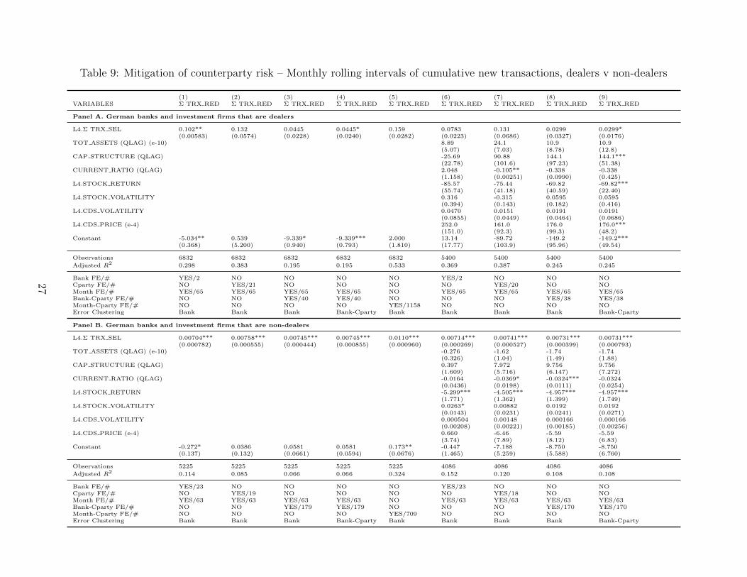
Table 9: Mitigation of counterparty risk – Monthly rolling intervals of cumulative new transactions, dealers v non-dealers
(1) (2) (3) (4) (5) (6) (7) (8) (9)VARIABLES Σ TRX RED Σ TRX RED Σ TRX RED Σ TRX RED Σ TRX RED Σ TRX RED Σ TRX RED Σ TRX RED Σ TRX RED
Panel A. German banks and investment firms that are dealers
L4.Σ TRX SEL 0.102** 0.132 0.0445 0.0445* 0.159 0.0783 0.131 0.0299 0.0299*(0.00583) (0.0574) (0.0228) (0.0240) (0.0282) (0.0223) (0.0686) (0.0327) (0.0176)
TOT ASSETS (QLAG) (e-10) 8.89 24.1 10.9 10.9(5.07) (7.03) (8.78) (12.8)
CAP STRUCTURE (QLAG) -25.69 90.88 144.1 144.1***(22.78) (101.6) (97.23) (51.38)
CURRENT RATIO (QLAG) 2.048 -0.105** -0.338 -0.338(1.158) (0.00251) (0.0990) (0.425)
L4.STOCK RETURN -85.57 -75.44 -69.82 -69.82***(55.74) (41.18) (40.59) (22.40)
L4.STOCK VOLATILITY 0.316 -0.315 0.0595 0.0595(0.394) (0.143) (0.182) (0.416)
L4.CDS VOLATILITY 0.0470 0.0151 0.0191 0.0191(0.0855) (0.0449) (0.0464) (0.0686)
L4.CDS PRICE (e-4) 252.0 161.0 176.0 176.0***(151.0) (92.3) (99.3) (48.2)
Constant -5.034** 0.539 -9.339* -9.339*** 2.000 13.14 -89.72 -149.2 -149.2***(0.368) (5.200) (0.940) (0.793) (1.810) (17.77) (103.9) (95.96) (49.54)
Observations 6832 6832 6832 6832 6832 5400 5400 5400 5400
Adjusted R2 0.298 0.383 0.195 0.195 0.533 0.369 0.387 0.245 0.245
Bank FE/# YES/2 NO NO NO NO YES/2 NO NO NOCparty FE/# NO YES/21 NO NO NO NO YES/20 NO NOMonth FE/# YES/65 YES/65 YES/65 YES/65 NO YES/65 YES/65 YES/65 YES/65Bank-Cparty FE/# NO NO YES/40 YES/40 NO NO NO YES/38 YES/38Month-Cparty FE/# NO NO NO NO YES/1158 NO NO NO NOError Clustering Bank Bank Bank Bank-Cparty Bank Bank Bank Bank Bank-Cparty
Panel B. German banks and investment firms that are non-dealers
L4.Σ TRX SEL 0.00704*** 0.00758*** 0.00745*** 0.00745*** 0.0110*** 0.00714*** 0.00741*** 0.00731*** 0.00731***(0.000782) (0.000555) (0.000444) (0.000855) (0.000960) (0.000269) (0.000527) (0.000399) (0.000793)
TOT ASSETS (QLAG) (e-10) -0.276 -1.62 -1.74 -1.74(0.326) (1.04) (1.49) (1.88)
CAP STRUCTURE (QLAG) 0.397 7.972 9.756 9.756(1.609) (5.716) (6.147) (7.272)
CURRENT RATIO (QLAG) -0.0164 -0.0369* -0.0324*** -0.0324(0.0436) (0.0198) (0.0111) (0.0254)
L4.STOCK RETURN -5.299*** -4.505*** -4.957*** -4.957***(1.771) (1.362) (1.399) (1.749)
L4.STOCK VOLATILITY 0.0263* 0.00882 0.0192 0.0192(0.0143) (0.0231) (0.0241) (0.0271)
L4.CDS VOLATILITY 0.000504 0.00148 0.000166 0.000166(0.00208) (0.00221) (0.00185) (0.00256)
L4.CDS PRICE (e-4) 0.660 -6.46 -5.59 -5.59(3.74) (7.89) (8.12) (6.83)
Constant -0.272* 0.0386 0.0581 0.0581 0.173** -0.447 -7.188 -8.750 -8.750(0.137) (0.132) (0.0661) (0.0594) (0.0676) (1.465) (5.259) (5.588) (6.760)
Observations 5225 5225 5225 5225 5225 4086 4086 4086 4086
Adjusted R2 0.114 0.085 0.066 0.066 0.324 0.152 0.120 0.108 0.108
Bank FE/# YES/23 NO NO NO NO YES/23 NO NO NOCparty FE/# NO YES/19 NO NO NO NO YES/18 NO NOMonth FE/# YES/63 YES/63 YES/63 YES/63 NO YES/63 YES/63 YES/63 YES/63Bank-Cparty FE/# NO NO YES/179 YES/179 NO NO NO YES/170 YES/170Month-Cparty FE/# NO NO NO NO YES/709 NO NO NO NOError Clustering Bank Bank Bank Bank-Cparty Bank Bank Bank Bank Bank-Cparty
27
longer horizons as revealed by Panels A in Tables 8 and 9.
One way to interpret the results in Tables 8 and 9 is that the accumulation of counterparty
risk might be slower for non-dealers in comparison to that of dealers. Non-dealers might be
waiting to hedge until the open interest hits a certain level or ratio, and this might be the
reason why they hedge less frequently. Another possibility might be the lower turnus of risk
management meetings at non-dealer institutions, which could fix hedging action deadlines to
a less frequent extent.
4.3 Identification through an Exogenous Shock on the Underlying
The previous two subsections made use of the transaction-level CDS dataset together with
bank, counterparty or bank-counterparty pair fixed effects, and relied on time (week/month)
or counterparty-time pair fixed effects to address any endogeneity that could have been caused
by aggregate or counterparty-specific time-variant factors, which may simultaneously drive
protection bought from the global dealer today and protection bought on the global dealer
on a future week or month.
An alternative robust way to address this issue is to make use of price shocks on under-
lyings, whose protection are being purchased by our sample banks and financial institutions
from the global counterparties at the SEL time step. An ideal identification could be achieved
through looking at the CDS price change of each underlying u in all trading activities between
the German banks and their counterparties, and multiplying this value with the current net
position of the same bank i with the same counterparty j on this underlying u (“NETSEL-
POS”). The value in Equation 3 could be viewed as an individual shock (“INDSHOCK”) to
the counterparty risk of the bank with respect to a given underlying u.
INDSHOCKi,j,u,t = NETSELPOSi,j,u,t−1 ∗ (CDS PRICEu,t − CDS PRICEu,t−1) (3)
In order to reach the aggregate shock to the counterparty risk of a bank with respect to all
underlyings, the individual shocks in Equation 3 could be aggregated across all underlyings
28
u that are traded between a bank-counterparty pair.
SHOCKi,j,t =u∑INDSHOCKi,j,u,t (4)
The variable SHOCKi,j,t provides a valuable exogenous shock on counterparty risk of
bank i on counterparty j, which enables the consecutive actions of bank i on trading the
CDS of counterparty j to be independently interpreted from any endogeneity. Table 10
Panel A introduces ΣSHOCKi,j,t as a new explanatory variable, where past four weeks
of price shocks on all underlyings are aggregated. In the first (second) part of the panel
the dependent variable is the cumulative number of new protection contracts,“TRX RED”
(cumulative volume of new protection, “VOL RED”) purchased on the counterparty dur-
ing the immediately following four weeks. We make use of the following specifications in
Equations 5 and 6, alternatively with (1) bank and month FE, (2) counterparty and month
FE, and (3) counterparty-month pair FE. The fourth and fifth specifications add the typical
counterparty-specific controls that were used previously into specifications (1) and (2).
4∑k=1
TRX REDi,j,t+k = a0 + a1
3∑k=0
SHOCKi,j,t−k + a2Xj,t + FE + εi,j,t (5)
4∑k=1
V OL REDi,j,t+k = a0 + a1
3∑k=0
SHOCKi,j,t−k + a2Xj,t + FE + εi,j,t (6)
The results in Table 10 Panel A indicate that both dependent variables, number of new
contracts and notional amount purchased on the counterparty, are explained by the exogenous
increase in the counterparty risk of the global dealer, revealed by the price shock on the CDS
underlyings in prior weeks. In economic terms, a 100 bps aggregate CDS price deterioration
(increase) in 10 EUR billion of an aggregate net sold position to the counterparty results in
purchase of 3.25-6.69 additional contracts bought on the counterparty in order to mitigate
the counterparty risk emerging from the price shock. Similarly, the second part of Panel A
reveals that the same conditions result in a protection purchase of 18.5-38.7 EUR million on
29
the counterparty.9
Panel B shows the effects of weekly price shocks on our sample banks’ behaviour on pur-
chase of protection on the counterparty (Equations 7 and 8). The same pattern of mitigation
of counterparty risk due to exogenous price shocks on the underlying are once again observed,
albeit at a lesser economic extent.
TRX REDi,j,t+1 = a0 + a1SHOCKi,j,t + a2Xj,t + FE + εi,j,t (7)
V OL REDi,j,t+1 = a0 + a1SHOCKi,j,t + a2Xj,t + FE + εi,j,t (8)
Overall, the results in this section underline once again the robustness of the results when
an exogenous shock is used for a better identification.
4.4 Robustness
This section provides the results for alternative monthly and weekly specifications. We
specifically look at whether German banks hedge their counterparty risk from correct parties
(no wrong-way risk), and whether results are robust when (i) contemporaneous months and
weeks of hedging activity are analyzed, and (ii) non-overlapping monthly specifications are
used.10 Table 11 reports the results of these checks by tabulating only the main variable of
interest for monthly and weekly specifications in Panels A and B, respectively.
4.4.1 Wrong-Way Risk
“Wrong-way risk” arises when banks intend to mitigate their counterparty risk through the
purchase of protection on their counterparty from a third party that is highly correlated
with their initial counterparty. For instance, if a German bank purchases protection on a
Japanese counterparty from another Japanese third party, it can be suggested that wrong-
way risk mitigation occurs. In order to see whether German financial institutions mitigate
9A one standard deviation shock would have a value of 62.8 billion, which is a value close to this scenario.10In undocumented results, our main finding is shown to be also robust when only observations of non-zero
hedging activity are utilized.
30
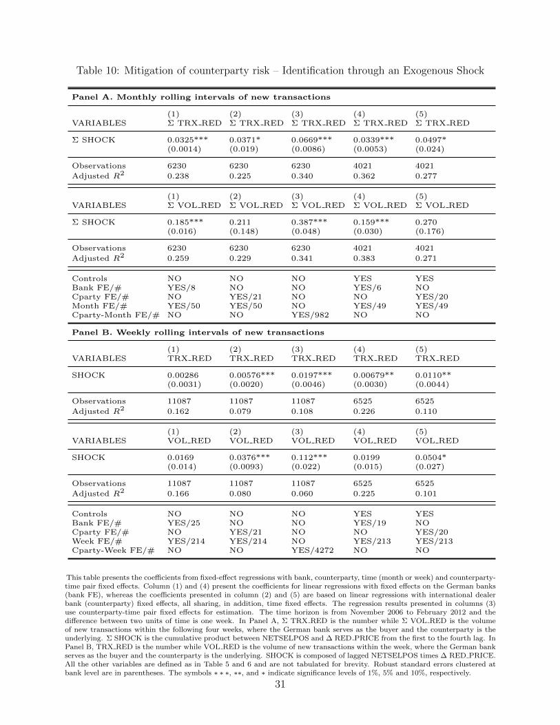
Table 10: Mitigation of counterparty risk – Identification through an Exogenous Shock
Panel A. Monthly rolling intervals of new transactions
(1) (2) (3) (4) (5)VARIABLES Σ TRX RED Σ TRX RED Σ TRX RED Σ TRX RED Σ TRX RED
Σ SHOCK 0.0325*** 0.0371* 0.0669*** 0.0339*** 0.0497*(0.0014) (0.019) (0.0086) (0.0053) (0.024)
Observations 6230 6230 6230 4021 4021
Adjusted R2 0.238 0.225 0.340 0.362 0.277
(1) (2) (3) (4) (5)VARIABLES Σ VOL RED Σ VOL RED Σ VOL RED Σ VOL RED Σ VOL RED
Σ SHOCK 0.185*** 0.211 0.387*** 0.159*** 0.270(0.016) (0.148) (0.048) (0.030) (0.176)
Observations 6230 6230 6230 4021 4021
Adjusted R2 0.259 0.229 0.341 0.383 0.271
Controls NO NO NO YES YESBank FE/# YES/8 NO NO YES/6 NOCparty FE/# NO YES/21 NO NO YES/20Month FE/# YES/50 YES/50 NO YES/49 YES/49Cparty-Month FE/# NO NO YES/982 NO NO
Panel B. Weekly rolling intervals of new transactions
(1) (2) (3) (4) (5)VARIABLES TRX RED TRX RED TRX RED TRX RED TRX RED
SHOCK 0.00286 0.00576*** 0.0197*** 0.00679** 0.0110**(0.0031) (0.0020) (0.0046) (0.0030) (0.0044)
Observations 11087 11087 11087 6525 6525
Adjusted R2 0.162 0.079 0.108 0.226 0.110
(1) (2) (3) (4) (5)VARIABLES VOL RED VOL RED VOL RED VOL RED VOL RED
SHOCK 0.0169 0.0376*** 0.112*** 0.0199 0.0504*(0.014) (0.0093) (0.022) (0.015) (0.027)
Observations 11087 11087 11087 6525 6525
Adjusted R2 0.166 0.080 0.060 0.225 0.101
Controls NO NO NO YES YESBank FE/# YES/25 NO NO YES/19 NOCparty FE/# NO YES/21 NO NO YES/20Week FE/# YES/214 YES/214 NO YES/213 YES/213Cparty-Week FE/# NO NO YES/4272 NO NO
This table presents the coefficients from fixed-effect regressions with bank, counterparty, time (month or week) and counterparty-time pair fixed effects. Column (1) and (4) present the coefficients for linear regressions with fixed effects on the German banks(bank FE), whereas the coefficients presented in column (2) and (5) are based on linear regressions with international dealerbank (counterparty) fixed effects, all sharing, in addition, time fixed effects. The regression results presented in columns (3)use counterparty-time pair fixed effects for estimation. The time horizon is from November 2006 to February 2012 and thedifference between two units of time is one week. In Panel A, Σ TRX RED is the number while Σ VOL RED is the volumeof new transactions within the following four weeks, where the German bank serves as the buyer and the counterparty is theunderlying. Σ SHOCK is the cumulative product between NETSELPOS and ∆ RED PRICE from the first to the fourth lag. InPanel B, TRX RED is the number while VOL RED is the volume of new transactions within the week, where the German bankserves as the buyer and the counterparty is the underlying. SHOCK is composed of lagged NETSELPOS times ∆ RED PRICE.All the other variables are defined as in Table 5 and 6 and are not tabulated for brevity. Robust standard errors clustered atbank level are in parentheses. The symbols ∗ ∗ ∗, ∗∗, and ∗ indicate significance levels of 1%, 5% and 10%, respectively.
31
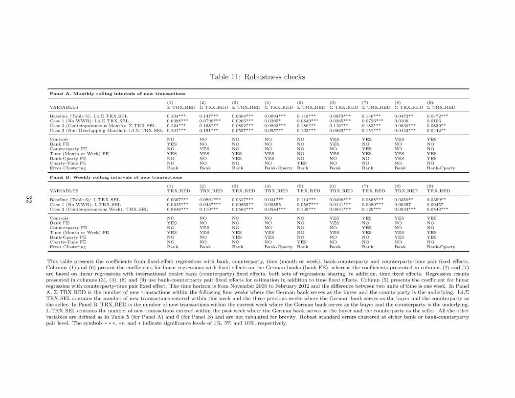
Table 11: Robustness checks
Panel A. Monthly rolling intervals of new transactions
(1) (2) (3) (4) (5) (6) (7) (8) (9)VARIABLES Σ TRX RED Σ TRX RED Σ TRX RED Σ TRX RED Σ TRX RED Σ TRX RED Σ TRX RED Σ TRX RED Σ TRX RED
Baseline (Table 5): L4.Σ TRX SEL 0.104*** 0.147*** 0.0694*** 0.0694*** 0.148*** 0.0873*** 0.146*** 0.0472** 0.0472***Case 1 (No WWR): L4.Σ TRX SEL 0.0398*** 0.0798*** 0.0205*** 0.0205* 0.0849*** 0.0265*** 0.0726*** 0.0106 0.0106Case 2 (Contemporaneous Month): Σ TRX SEL 0.124*** 0.168*** 0.0892*** 0.0892*** 0.180*** 0.116*** 0.182*** 0.0830*** 0.0830**Case 3 (Non-Overlapping Months): L4.Σ TRX SEL 0.101*** 0.151*** 0.0557*** 0.0557** 0.162*** 0.0863*** 0.151*** 0.0442*** 0.0442**
Controls NO NO NO NO NO YES YES YES YESBank FE YES NO NO NO NO YES NO NO NOCounterparty FE NO YES NO NO NO NO YES NO NOTime (Month or Week) FE YES YES YES YES NO YES YES YES YESBank-Cparty FE NO NO YES YES NO NO NO YES YESCparty-Time FE NO NO NO NO YES NO NO NO NOError Clustering Bank Bank Bank Bank-Cparty Bank Bank Bank Bank Bank-Cparty
Panel B. Weekly rolling intervals of new transactions
(1) (2) (3) (4) (5) (6) (7) (8) (9)VARIABLES TRX RED TRX RED TRX RED TRX RED TRX RED TRX RED TRX RED TRX RED TRX RED
Baseline (Table 6): L.TRX SEL 0.0607*** 0.0891*** 0.0317*** 0.0317** 0.114*** 0.0496*** 0.0858*** 0.0359** 0.0359**Case 1 (No WWR): L.TRX SEL 0.0215*** 0.0437*** 0.00855** 0.00855 0.0587*** 0.0141*** 0.0380*** 0.00457 0.00457Case 2 (Contemporaneous Week): TRX SEL 0.0848*** 0.110*** 0.0584*** 0.0584*** 0.138*** 0.0841*** 0.129*** 0.0543*** 0.0543***
Controls NO NO NO NO NO YES YES YES YESBank FE YES NO NO NO NO YES NO NO NOCounterparty FE NO YES NO NO NO NO YES NO NOTime (Month or Week) FE YES YES YES YES NO YES YES YES YESBank-Cparty FE NO NO YES YES NO NO NO YES YESCparty-Time FE NO NO NO NO YES NO NO NO NOError Clustering Bank Bank Bank Bank-Cparty Bank Bank Bank Bank Bank-Cparty
This table presents the coefficients from fixed-effect regressions with bank, counterparty, time (month or week), bank-counterparty and counterparty-time pair fixed effects.Columns (1) and (6) present the coefficients for linear regressions with fixed effects on the German banks (bank FE), whereas the coefficients presented in columns (2) and (7)are based on linear regressions with international dealer bank (counterparty) fixed effects, both sets of regressions sharing, in addition, time fixed effects. Regression resultspresented in columns (3), (4), (8) and (9) use bank-counterparty pair fixed effects for estimation in addition to time fixed effects. Column (5) presents the coefficient for linearregression with counterparty-time pair fixed effect. The time horizon is from November 2006 to February 2012 and the difference between two units of time is one week. In PanelA, Σ TRX RED is the number of new transactions within the following four weeks where the German bank serves as the buyer and the counterparty is the underlying. L4.ΣTRX SEL contains the number of new transactions entered within this week and the three previous weeks where the German bank serves as the buyer and the counterparty asthe seller. In Panel B, TRX RED is the number of new transactions within the current week where the German bank serves as the buyer and the counterparty is the underlying.L.TRX SEL contains the number of new transactions entered within the past week where the German bank serves as the buyer and the counterparty as the seller. All the othervariables are defined as in Table 5 (for Panel A) and 6 (for Panel B) and are not tabulated for brevity. Robust standard errors clustered at either bank or bank-counterpartypair level. The symbols ∗ ∗ ∗, ∗∗, and ∗ indicate significance levels of 1%, 5% and 10%, respectively.
32

counterparty risk keeping in mind the need to avoid wrong-way risk, we remove all the same
country hedging activity and see if the results still hold. Hence, all protection purchases on,
e.g., US dealers, from another US financial institution, are removed from the sample. Cases
1 in Panels A and B of Table 11 show that although the hedge proportion is lower, there is
indeed significant evidence for German financial institutions to be avoiding wrong-way risk
mitigation.
4.4.2 Contemporaneous months and weeks
It could be argued that risk-mitigation activity takes place directly in the same weeks or
months whenever counterparty risk occurs, due to immediate reaction of the dealer desks.
Cases 2 in Panels A and B of Table 11 provide evidence that risk mitigation takes place
even in the contemporaneous months and weeks. Interestingly, the hedge proportion is much
higher when compared to baseline results in Tables 5 and 6, which gives rise to the possibility
that risk mitigation is immediately undertaken as well.
4.4.3 Non-overlapping months
One argument could be that the results might be spurious due to autocorrelated usage of
weeks in monthly rolling intervals. If overlapping weeks are rolled over, double counting
of information might emerge. In order to avoid this concern, Case 3 in Panel A of Table
11 generates results with non-overlapping rolling of monthly intervals. The coefficients of
interest indicate an even slightly higher hedge proportion in some specifications compared to
the baseline results in Table 5.
5 Conclusion and Policy Implications
This paper provides initial evidence of counterparty risk-mitigation activity on the part of
financial institutions. Our sample banks and financial institutions manage their counterparty
risk on weekly or monthly horizons as evidenced both by transaction-level and position-level
information. Trading-intensive dealer banks are found to be more active in hedging, over
both short and longer horizons, whereas non-dealer banks appear to manage this risk only
33

over longer, monthly intervals. Higher stock return and CDS price volatility, lower past stock
returns, and higher CDS prices of the counterparty are shown to boost hedging behaviour on
the counterparty. The sample banks are also shown to mitigate their counterparty risk by
keeping in mind to avoid wrong-way hedging. Finally, we further document the robustness
of our main finding through identifying the risk mitigation activity when an exogenous price
shock increases the counterparty risk of our sample banks.
The analysis provided in this study has implications regarding the ongoing debate on
regulating the OTC market and further phasing in central clearing, which would seemingly
eliminate the necessity of bilateral trading and diminish counterparty risk. We show that
risk-mitigation is taking place in the OTC market despite the high level of collateralization
indicated by recent studies, and that purchasing protection on the reference entities of coun-
terparties seems to be a reliable method in circumstances where collateral alone provides
insufficient protection. Players in the market are able to tentatively hedge their counterparty
risk through CDSs in the OTC market regardless of whether they are a central clearing
member. Given that we are able to show evidence on hedging in the CDS market that en-
compasses only a part of counterparty risk-taking activity, we expect that even a much higher
degree of counterparty risk mitigation could be evidenced if exposures from interest rate and
FX swaps were included. Altogether, the analysis in the paper points to an additional cost
of not having central clearing, which has not been articulated in the literature.
We argue in this study that regulatory capital relief motives could actively accentuate
this type of risk mitigation. Since Basel III and its European implementation, the CRR,
explicitly formulate that any protection purchase on the counterparty would diminish the
required regulatory CVA capital, future work should study whether such an incentive might
create adverse effects that lead to excessive risk-taking. In the end, it is in the best interest
of regulators to set the right incentives for market participants and clearing houses for an
optimal design of the capital regulation of CDSs.
34
References
Acharya, V. and A. Bisin (2014). Counterparty risk externality: Centralized versus over-the-counter markets. Journal of Economic Theory 149, 153–182.
Acharya, V. V., Y. Gunduz, and T. C. Johnson (2017). Bank use of sovereign CDS in theEurozone crisis: Hedging and risk incentives.
Arora, N., P. Gandhi, and F. A. Longstaff (2012). Counterparty credit risk and the creditdefault swap market. Journal of Financial Economics 103, 280–293.
Augustin, P., M. G. Subrahmanyam, D. Y. Tang, and S. Q. Wang (2014). Credit defaultswaps: A survey. Foundations and Trends in Finance 9, 1–196.
Basel Committee on Banking Supervision (2011). Basel III: A Global regulatory frameworkfor more resilient banks and banking systems. Technical report,, Bank for InternationalSettlements.
Biais, B., F. Heider, and M. Hoerova (2016). Risk-sharing or risk-taking? counterparty risk,incentives, and margins. The Journal of Finance, 71(4), 1669–1698.
Biswas, G., S. Nikolova, and C. W. Stahel (2015). The Transaction costs of trading corporatecredit. Working Paper .
Capital Requirements Regulation (CRR) (2013). Regulation (eu) no. 575/2013 of the euro-pean parliament and of the council. Official Journal of the European Union.
Cooper, I. and A. Mello (1991). The default risk of swaps. The Journal of Finance 46 (2),597–620.
Du, W., S. Gadgil, M. B. Gordy, and C. Vega (2016). Counterparty risk and counterpartychoice in the credit default swap market. Finance and Economics Discussion Series 087,Washington: Board of Governors of the Federal Reserve System.
Duffie, D. and M. Huang (1996). Swap rates and credit quality. The Journal of Finance 51 (3),921–949.
Duffie, D., M. Scheicher, and G. Vuillemey (2015). Central clearing and collateral demand.Journal of Financial Economics 116 (2), 237–256.
Duffie, D. and H. Zhu (2011). Does a central clearing counterparty reduce counterparty risk?Review of Asset Pricing Studies 1 (1), 74–95.
Gehde-Trapp, M., Y. Gunduz, and J. Nasev (2015). The liquidity premium in cds transactionprices: Do frictions matter? Journal of Banking & Finance, 61, 184–205.
Gunduz, Y., S. Ongena, G. Tumer-Alkan, and Y. Yu (2017). CDS and credit: Testingthe small bang theory of the financial universe with micro data. Deutsche BundesbankDiscussion Paper No:16/2017, AFA 2017 Chicago Meetings Paper .
35
Hull, J. and A. White (2001). Valuing credit default swaps ii: Modeling default correlations.Journal of Derivatives 8, 12–22.
Jarrow, R. A. and F. Yu (2001). Counterparty risk and the pricing of defaultable securities.The Journal of Finance 56 (5), 1765–1799.
Klingler, S. and D. Lando (2015). Safe-haven CDS premia. Working paper .
Kraft, H. and M. Steffensen (2007). Bankruptcy, counterparty risk, and contagion. Reviewof Finance 11, 209–252.
Loon, Y. C. and Z. K. Zhong (2014). The Impact of central clearing on counterparty risk,liquidity, and trading: Evidence from the credit default swap market. Journal of FinancialEconomics 112, 91–115.
Oehmke, M. and A. Zawadowski (2017). The anatomy of the cds market. Review of FinancialStudies, 30(1), 80–119.
Peltonen, T. A., M. Scheicher, and G. Vuillemey (2014). The network structure of the cdsmarket and its determinants. Journal of Financial Stability 13, 118–133.
Shachar, O. (2012). Exposing the exposed: Intermediation capacity in the credit defaultswap market. Working Paper .
Yorulmazer, T. (2013). Has financial innovation made the world riskier? CDS, regulatoryarbitrage and systemic risk. Working paper .
36