MIXING OF FLUIDS AND SOLIDS

Julio M. OttinoDepartment of Chemical Engineering

Northwestern UniversityEvanston, Illinois 60208-3120

Phone: 847-491-3558FAX: 847-491-3728

e-mail: ottino@chem-eng. nwu.edu

.

ABSTRACI’

The work reported here focuses on mixing of fluids and mixing of solids; bothareas involving theory and experiments. Within mixing of fluids we consider viscousmixing in 3D flows and mixing and dispersion of immiscible fluids. In the mixing ofsolids area we consider simultaneous mixing and segregation of powders in tumblingsystems; the tools in this area being particle dynamics and Monte Carlo simulations,continuum and geometrical descriptions. The fluid aspects are reaching maturity; thesolids area is newer and significant inroads have been made in the last two yearsespecially in problems involving competition between mixing and segregation; the bulkof the attention is given to this area.

INTRODUCTION

Mixing is so widespread in technology and nature that one might expect that acomprehensive theory would have been developed in be gained by a unified approach and bycontrasting extremes, in this case mixing of fluids and mixing of dry powders. This idea is notnew. The first views -- and vocabulary -- of solid mixing were based on analogies with mixingof fluids.” Recent developments provide clues for cross-fertilization. For example, under certaincircumstances, both problems -- mixing of fluids and mixing of powders -- can be described bymaps. And, as we demonstrate, chaos concepts which proved useful in the analysis of mixing offluids, apply also to solid mixing.

MIXING OF FLUIDS

A complete description of the mixing of fluids is far from trivial and may well never beattained. The underlying physical processes are however clear. Exceptions notwithstanding, theNavier-Stokes equations govern flow; diffusional processes, if present, are well described byFicks law; interracial conditions by the Young-Laplace equation, and so on. The stumblingblock was that, until recently, it was unclear how to apply the considerable mathematicalapparatus of fluid mechanics to mixing.

The 2D picture is now clear: Dye structures in time-periodic flows evolve in an iterativefashion: an entire structure is mapped into a new structure with persistent large-scale features and

71

with finer and finer scale features revealed at each period of the flow. The 3D picture isconsiderably less clear. Another issue is that the bulk of mixing work to date has been for thecase of single-phase fluids. Much remains to be done for the case of two-phase systems.

MIXING OF SOLIDS

It may naively be argued that, as in the case of the mixing of fluids, the underlyingphysical processes governing granular mixing are clear as well -- one knows how particlesinteract: normal forces are Hertzian, tangential forces are Coulombic, etc. This is misleading.Little is knc~wn about cooperative phenomena and it is at this length scale that granular materialspart company with their fluid counterparts; averaging, the cornerstone of continuum fielddescriptions, may not work. But probably the most crucial difference is segregation:. Ingranular materials mixing and segregation come together. In solids, more “agitation” does notimply better mixing. Granular mixtures of dissimilar (and not-too-dissimilar) materials oftensegregate when shaken or tumbled. Thus, for exampIe, differences in size result in percolationof smaller particles in flowing layers 1, differences in size 2 or densi~ 3 result in radial and axialsegregation.

PROGRAM’S PHILOSOPHY: WHY FOCUS ON MIXING?

Why focus on mixing? Inarguably the first part of the answer has to do with thepractical implications of the results. A second aspect is somewhat less obvious, and applies toboth fluids and solids. Consider the case of solids, which is probably somewhat more dramatic.Solutions of flow problems for granular materials are rare, and there are only few instances ofdirect coml?arison of theoretical predictions to experimental results. Mixing experiments, incontrast, generate over long times large scale patterns and structures which can be easilyvisualized. (see for example 4). Thus mixing studies provide a means of studying mechanismsof flows which are otherwise difficult to probe experimentally. There is another aspect as well: afailure to capture large scale phenomena serves as a litmus test of theories and computationalmodels.

FLUID MIXING AND SOLID MIXING ANALOGIES

As discussed earlier, under certain circumstances both mixing of fluids and mixing ofsolids can be described by maps. This is true :for example when mixing of solids proceeds byavalanches,, This idea leads to several applications.5 Other analogies can be readily exploited aswell. Fluid mixing theory says that steady 21) flows are poor mixers. Thus one may easilydeduce that powder mixing occurs more “slowly” in the continuous steady flow regime than inthe discrete, time-periodic, avalanching case: it takes more rotations to achieve the same mixingin the continuous flow regime. The question is then how to make the continuous flow chaotic.Another example is the case of 3D cylinders. Axial mixing, essentially diffusive, is very slow.Chaos concepts are useful again: Faster overall mixing can be achieved by a combination ofavalanches: rotation and “wobbling” of the axis of the cylinder.

Mixing in 3D Flows

A t,~pic of current interest is complex,3D flOWS; this is an area were there is an imbalancetowards computations,G Figure 1 shows some of our preliminary results in a system that we callthe “fundamental mixing tank”. Our philosophy here is that rather than going towards realism

and try to simulate an actual stirred tank we conduct controlled experiments and high precision

““ “

The ratio of deforming viscous forces to resisting interracial tension forces in the case of

computations in a system that contains the essential elements of a full tank, as shown in Figure 1.All indications are that we have a good match between experiment and computations and weexpect that this system will become a paradigm for and inspire advances on theoreticaldescriptions of mixing.

Mixing of Immiscible Fluids and Dispersion

Mixing and dispersion of viscous fluids -- blending in the polymer processing literature --is the result of complex interaction between flow and events occurring at drop length-scales:breakup, coalescence and hydrodynamic interactions. Similarly, mixing and dispersion ofpowdered solids in viscous liquids is the result of complex interaction between flow and events-- erosion, fragmentation and aggregation -- occurring at agglomerate Iength scales.Important applications of these processes include the compounding of molten polymers, and thedispersion of fine particles in polymer melts. The foIlowing analogies are apparent:

breakup #fragmentation

coalescence ++a.wre~ation

droplets is the capillary nu%ber, Ca. Similarly, the”ratio of viscous to cohesive forces inagglomerates is the fragmentation number, Fa. Thus Ca<O ( 1) and Fa<O( 1) determineconditions where no breakup or fragmentation is possible. Both processes, breakup andcoalescence, for drops, and fragmentation and aggregation, for solids, lead to time-varyingdistributions of drops and cluster sizes which become time-invariant when scaled in suitableways. Two areas have been pursued -- breakup and coalescence of immiscible fluids, andaggregation and fragmentation of solids in viscous liquids. The primary objective of our work inthis area is to pursue both topics in parallel highlighting connections as to increaseunderstanding. Self-similarity is common to all these problems; exampies arise in the context ofthe distribution of stretching within chaotic flows, in the asymptotic evolution of fragmentationprocesses, and in the equilibrium distribution of drop sizes generated upon mixing of immisciblefluids. A comprehensive summary of our results appears in 7 and 8.

1 Mixing and Segregation of Solids

~ Studies in this area involve the confluence of several tools: Monte Carlo simulations, thisbeing restricted to flowing layers, particle dynamics, and constitutive based continuumdescriptions.

Particle Dynamics

Particle dynamics methods (PD) 9’10are eminently suited to study mixing and segregation-- particle properties can be varied on a particle-by-particle basis, allowing close matchingbetween computations and experiments. In addition detailed mixed structures are easily capturedand visualized. This method, however, is computationally intensive. These techniques havebeen used in two different ways:

● Studies of segregation in flowing layers. These studies are used to investigate constitutivemodels for segregation fluxes.

● Studies of mixing systems in terms of “hybrid” techniques.

73

[a)

(b)

Figure 1 – Area below the impeller for the fundamental mixing tank. Impellerangle=14.3°,Re=7.0. (a) Experimentalcross sectionalphoto of the flow illuminatedwitha sheet of laser light (white band is impeller location),and (b) the numericalPoincardsection.

Monte Carlo Simulations

An alternative to PD methods -- and a much less time (or CPU) consuming way -- ofstudying segregation is by means of Monte Carlo techniques.’1 ~12~13~14~15While the results ofMonte Carlo simulations only approximately describe the actual physical system (particles areassumed to be perfectly elastic), they yield goc}d agreement with PD simulations when used toinvestigate constitutive descriptions of segregation fluxes in flowing layers.

Hybrid Simulations

In many cases of practical interest -- such as in a tumbler mixer, where the bulk of theparticle motion consists of a solid body rotation -- it is not necessary to explicitly calculate themotion of all of the particles. By combining particle dynamics and geometrical insight -- inessence, by focusing the particle dynamics simulation only where it is needed -- a new hybridmethod of simulation, which is much faster than a conventional particle dynamics method, hasbeen devised. This technique can yield, according to flow conditions, up to more than an orderof magnitude increase in computational speed. This allows simulations of the order of 104particles on a typical workstation (see Figure 216). Segregation problems in mixers with realisticdiameter to particle size ratios can thus be studied.

Phenomenological Model of Segregatiori

We have proposed and tested the idea that, in the case of a mixture of particles withdifferent densities, the driving force for segregation can be described in terms of an effective“buoyant force.” The idea can be applied to a flowing layer and tested by means of computersimulations (PD and MC), and s~bsequently incorporated into models of competing mixing andsegregation in rotating tumblers. Denote by J,Ythe segregation flux of the more dense particlesand by $1 the volume of the denser particles. The segregation flux is

.

J,Y = –C$l (pl – (p))gcosO(1)

where the average density is given by

(p) = P,o, +P202

0, +Q2

(2)

balance equation for steady flow down an inclined plane resulting from a balance betweensegregation and diffusion in the layer at equilibrium isand C is an unknown function which is ameasure of the resistance to local motion. The species

d

( 1— –D$,:+J,Y =0dz

(3)

where z is he direction normal to the flow, f=$l/@t, is the volume fraction of the more denseparticles, @ = ($1 + $Z)is the total solids volume fraction, D is the diffusivity and J,Y is thesegregation flux of the more dense particles. Substituting the heuristic buoyancy flow intoequation (3) and integrating yields the equilibrium volume fraction profile

()fIn —()

–~(1–~)Z+ln & (4)l–f = —o

where KS is the characteristic segregation velocity (a key assumption made while obtaining theabove equation is that the ratio (K@) is constant across the layer). Thus a plot of In(f/l-f)versus distanceprediction.

should produce a straight line. Both PD and MC simulations verify this

75

“76

0.0

0.5

1.0

1.5

simulationexperiment

Figure 2: Hybrid Comparison of Mixing for Avalanching. A comparison of mixing in theavalmching regimeform experiment(left)mtisimulation (right)at&fferent times. From top tobottom are: the initial condition, afterone half revolution,after one revolution, and after one andone half revolution.

In principle the constitutive model can then be incorporated into a general description ofmixing and segregation,

(5)

where J = (J~X,J~Y)is the segregation flux of the more dense particles; actual simulations thoughare conducted by means of a Lagrangian approach. Consider one example of the application ofthe theory and the ability to reproduce experimental results. The objective is to homogenize aninitially segregated mixture. Figure 3 shows an example of such a process, in which an initiallysegregated state evolves to an equilibrium distribution. Time evolution computations show thatthe model captures interesting trends: often the system is better mixed at intermediate times; afterpartial mixing the system unrnixes. 18

a) experiment simulation

0.5

0.45

0.4

-“

0.35

0.3

b) revolutions

Figure 3: (a)Timeevolutionof the distributionof a mixtureof particlesof differentdensitywithrotationof the cylinderobtainedexperimentally(left) and fromtheory (right). Rotationalspeedof the cylinderis 3 r.p.m. D~ker particlesin the simulationshave higherdensity. (b}Variationof the intensity of segregationwith cylinder revolutions for the pictures in (a) obtained fromexperimentsandLagrangkiusimulations.

Chaotic advection, which has been central in advancing the understanding of thefundamentals ofliquidmixing3, is alsopresentjngranularflows. We demonstiatedthis ideaforthe case of mixing of similar cohesionless powders, when segregation effects are unimportant.When the cross-section of the rotating container is circular, the mean flow is time-independent,and the streamlines (lines tangent to mean velocity field) act as impenetrable barriers toconvective mixing. Is there any way to speed up the mixing by increasing the contribution ofconvection? Several studies of fluid flows show that time modulation of streamlines -- such thatthere are intersections between streamlines obtained at different times --is generally sufficient toproduce chaotic advection.3 In a rotating tumbler this simply happens when the cross-section isnot circular. We have demonstrated this idea in terms of computations in circular (as a referencecase) and elliptical containers and experiments and computations in square containers (Figure 4).

Figure 4: Comparisonof themixingof tracerparticlesin a circular,elliptical,andsquaremixersimulatedusingthemodelwithno particlediffusion. The inset figureon the upper left showsthePoincartlsection, and the initial condition i$ shown in the upper right inset. The cross-sectional231W21Sof the mixersareequalso that the amountof materialmixedin eachcaseis identical,as is therotationalspeedso that the mixingtimesare thesame.

ACKNOWLEDGMENT

This work has been supported by U.S. Department of Energy, Office of Basic EnergySciences, under grant DE-FG02-95ER14534, monitored by Dr. Robert Price.

REFERENCES

‘)Lacey, P. M., Developments in the theory of particle mixing, J. Appl. Chem., 4, 257-268(1954).

‘Savage, S. B. and Lun, C. K. K., Particle size segregation in inclined chute flow of drycohesionless granular materials, J. Fluid Mech., 189,311-335 (1988).

‘Donald, M. B. and Roseman, B., Mixing and dernixing of solid particles. Part 1. Mechanismsin a horizontal drum mixer, Brit. Chem.’ Erzg., 7, 749-753 (1962).

3Ristow, G. H., Particle mass segregation in an two-dimensional rotating drum, Europlzys.Lett., 28, 97-101 (1994).

‘Metcalfe, G., Shinbrot, T., McCarthy, J. J., and Ottino, J. M., Avalanche mixing of granularsolids, Nature, 374, 39-41 (1995).

5McCarthy, J. J., Shinbrot, T., Metcalfe, G., and Ottino, J.M., Mixing of granular materials inslowly rotated containers, AIChE J, 42, 3351-3363 (1996).

‘Tanguy, P. A., Lacroix, R., Bertrand, F., Choplin, L., and Brito-de La Fuente, E., Finteelement analysis of viscous mixing with an HRS impeller, AZChE J, 38, 939-944 (1992)

7J.M. Ottino, P. de Rousell, S. Hansen, and D.V. Khakhar, Mixing and Dispersion of ViscousFluids and Powdered Solids, Advances in Chemical Engineering, to appear 1998;

8S. Hansen, D.V. Kkakahr, and J.M. Ottino, Dispersion of Solids in Nonhomogeneous ViscousFlows, Chem. Eng. Sci. to appear 1998.

‘Campbell, C. S., and Brennen, C. E., Chute flows of granular material: some computersimulations. J. Appl. Mech. 52, 172-178 (1985).

10Cundall, P. A., and Strack, O. D. L., A discrete numerical model for granular assemblies.Geotechnique 29,47-65 (1979).

l’Moradi, M. and Rickayzen, The structure of a hard sphere fluid mixture confined to a slit,Molecular Phys., 66, 143-160 (1989).

“Tan, Z., Marini Bettolo Marconi, U., van Swol, F., and Gubbins, K. E., Hard-spheremixtures near a hard wall, J. Chem. Phys., 90, 3704-3712 (1989).

‘3Denton, A. R. and Ashcroft, N. W., Weighted density functional theory of non-uniform fluidmixtures: Application to the structure of ,binary hard sphere mixtures near a hard wall, Phys.Rev. A, 44, 8242-8248 (1991).

“Rosato, A., Prinz, F., Standburg, K. J., and Svendsen, R., Monte Carlo simulation ofparticulate matter segregation, Powder Technol., 49,59-69 (1986); Why Brazil nuts are ontop: size segregation of particulate matter by shaking, Phys. Rev. Lett., 58, 1038-1040(1987).

15Julien, R., Meakin, P., and Pavlovitch, A., Three-dimensional model for particle-sizesegregation by shaking, Phys. Rev. Lett., 69, 640-643 (1992).

“J.J. McCarthty and J.M. Ottino, Particle Dynamics Simulation; A Hybrid technique Applied toGranular Mixing, Powder Tech. submited 1997.

‘7D.V. Khakhar, J,J. McCarthy, T. Shinbrot, and J.M. Ottino, Transverse Flow and Mixing ofGranular Materials in A Rotating Cylinder, Phys. Fluids, 9,31-43 (1997).

18D.V. Khakhar, J.J. McCarthty, and J.M. Ottino, Radial Segregation of Granular Mixtures inRotating Cylinders, Phys. Fluids, 9,3600-3614 (1997)

7’9

TRANSPORT PROPERTIES OF POROUS MEDIAFROM THE MICROSTRUCTURE

S. Torquafio

Department of Civil Engineering & Operations Research and Princeton Materials InstitutePrinceton University, Princeton, N.J. 08544

ABSTRAICT

The determination of the effective transport properties of a random porousmedium remains a challenging area of research because the properties dependon the microstructure in a highly complex fashion. This paper reviews recenttheoretical and experimental progress that we have made on various aspects ofthis problem. A unified approach is taken to characterize the microstructureand the seemingly disparate properties of the medium.

I. INTRODUCTION

The purpose of this paper is to review progress that we have made in the last threeyears on five basic aspects of the problem of determining effective transport properties ofrandom porous media: (i) quantitative characterization of the microstructure of nontrivialmodels; (ii) 3D imaging of porous media using x-ray tomography; (iii) derivation of predictiveformulas on transport properties in terms of statistical correlation functions; (iv) derivation

of rigorous cross-property relations; (v) and reconstruction of porous media.

II. AVERAGED EQUATIONS

The random porous medium is a domain of space V(w) ~ 123 (where the realization$2 is taken from some probability space w) of volume V which is composed of two regions:the pore region VI(w) (in which transport occu:rs) of volume fraction (porosity) +1 and asolid-phase region V2(W) of volume fraction #2. Let 6’V be the surface between V] and V2.

The eflective conductivity a. is given by an iweraged Ohm’s law:

< J(x) >= O, <<E(x) > (1)

where < E(x) > and < J(x) > represent the ensemble average of the local electric andcurrent density fields, respectively. The local fields satisfy the usual steady-state conductionequations [1,2]. By mathematical analogy, results for u~ translate into equivalent results forthe thermal co:nductivit y, magnetic permeability y, dielectric constant, and diffusion coefficient.

The mean survival time T of a Brownian particle diffusing in the fluid phase of a porousmedium with a,n absorbing pore-solid interface is related to the average magnetization density

obtainable from a nuclear magnetic resonance (NMR) experiment [2,3]. ~ depends on theaverage pore size and diffusion coefficient D.

The fluid permeability k of a porous medium, defined by Darcy’s law,

< u(x) >= – ;VPO (x) , (2)

governs the rate at which a viscous fluid flows through it [4]. Here < u(x) > is the ensembleaverage of the local fluid velocity which satisfies the steady-state Stokes equations [5], VpO(x)is the applied pressure gradient, and p is the dynamic viscosity. k depends nontrivially on thepore geometry and may be regarded to be an eflective cross-sectional area of pore channels.

The e~ective elastic tensor C, is given by an averaged Hooke’s law:

< x(x) >= c, < t(x) > (3)

where < c(x) > and < X(x) > represent the ensen-dde average of the local strain and stressfields, respectively. The local fields satisfy the equilibrium equations [5]. The attenuation ofelastic waves in fluid-saturated porous media depends on their effective elastic moduli.

III. MICROSTRUCTURE CHARACTERIZATION

There are a variety of different types of statistical correlation functions that have arisenin rigorous expressions for transport properties. Until recently, application of such expres-

sions (although in existence for almost thirty years in some cases) was virtually nonexistentbecause of the difficulty involved in ascertaining the correlation functions.

A. Unified Theoretical Approach

For statistically inhomogeneous systems of N identical d-dimensional spheres, Torquato[6] has introduced the general n-point distribution function H.(xn; xp-~; r’) and found aseries representation of H. which enables one to compute it. From the general quantity H.one can obtain all of the correlation functions that arise in rigorous property relations andtheir generalizations. This formalism has been generalized to treat polydispersed spheres,anisotropic media (e.g., aligned ellipsoids and cylinders), and cell models.

The preponderance of previous studies have focused on statistically homogeneous media.Significantly less research has been devoted to the study of statistical~y inhomogeneous (non-ergodic) two-phase media and yet porous media frequently has this feature [5]. We haveproposed such a model consisting of inhomogeneous fully penetrable (Poisson distributed)spheres [7]. This model can be constructed for any specified variation of volume fraction (seeFig. 1) and permits one to evaluate the general n-point distribution function H.. Urdikethe case of statistically homogeneous media, the microstructure functions depend upon the

absolute positions of their arguments.

We have also studied the lineal path function [8] and cluster statistics [9,10] for the pro-totypical continuum percolation model of d-dimensional overlapping spheres. For d = 3, wehave computed the percolation threshold and critical exponents with heretofore unattainedaccuracy [11]. For the non-equilibrium random sequential addition process, we found exactexpressions for the nearest-neighbor functions for lamellar media [12]. The full distributionof local volume fraction fluctuations in models of random media have been evaluated [13].

(a) (b)

Figure 1: ExampIes of statistically inhomogeneous particles: system (a) is under an “anti-centrifugal” field and system (b) has a linear grade in the volume fraction.

We have studied fundamental questions pertaining to the structure of dense hard-spheresystems along the met astable amorphous branch via molecular dynamics simulations [14,15].For example, contrary to many previous studies, we found no existence of thermodynamicglass transition and found that the metastable system eventually crystallizes.

IV. 3D IMAGING VIA ‘TOMOGRAPHY

We have very recently obtained a high-resolution 3D digitized representation of a Foun-tainebleu sandstone (see Fig. 2) using synchrotron-based X-ray tomographic techniques [16].This digitized representation was used to extract a number of morphological characteristicsof the sample, including the pore-size functions (see Fig. 3), enabling us to predict thetransport properties of the rock. We have also employed the same technique to study themicrostructure and properties of a porous gel [17].

Figure 2: Surface cut (left) and pore space (right) of a 128 x 128 x 128 pixels sub-region ofthe Fontainebleau sandstone.

82

1.0

0.8

0.6

~

E6 0.4:

0.2

0.010 20 30 40 w

r(m)

Figure 3: Pore-size distribution function P(6) and the cumulative pore-size distributionfunction E’(6) for Fontainebleau sandstone.

V. MICROSTRUCTURE/PROPERTY CONNECTION

A. Rigorous Bounds

We have derived and computed bounds on the effective conductivity and elastic moduliof realistic models of random media which depend upon the microstructure through vari-ous sets of correlation functions and symmetry information [18-20]. We developed rigorousbounds on the effective conductivity o, of dispersions that are given in terms of the phasecontrast between the inclusions and matrix, the interjace properties, volume fraction, andhigher-order morphological information [21].

;z O Mcdel 1In 0.4 +Mcdel23 +?Model 3E.- ❑ Mcdel 4e x Model 5~ 0.2.-0 0Model 6

A Model 7V Model 8

0.00.0 0,1 0.2 0.3 0.4 0,5

Dir71eII$i0nleSSPoreSize Squared,+.2/7.0

Figure 4: Dimensionless mean survival time r/rO versus dimensionless mean pore size squared(6)2/rOD for all models 1-8. Solid curve is universal scaling relation.

83

0.0I I0.0 0.2 0.4 0.6 0,8 1.0

Fibervolumefraction,$,

Figure 5: Dimensionless effective transverse bulk modulus K./Kl vs. fiber volume fractiong$zfor random arrays of circular superrigid fibers in a compressible matrix. Note that theself-consistent (SC) formula violates the upper bc)und.

Guided by rigorous bounds on the mean survival time ~, we have found a universalscaling [22] for ~ (see Fig. 4) which is well represented by the simple expression

T 88—= –x + –X2,‘rO 57

(4)

where x = (J)2 /~0 D is the dimensionless mean pcjre size squared.

B. Exact Results

For the special case of periodic arrays, we have obtained exact results for the effectiveconductivity for both the interracial resistance case [23] and interracial conductance case [24].

We have derived new, exact series expansions for the effective elastic tensor of anisotropic,d-dimensional, two-phase disordered composites whose nth-order tensor coefficients are in-tegrals involving n-point correlation functions that characterize the structure (25,26]. Theseseries expansions, valid for any structure, perturb about certain optimal dispersions. Third-order truncation of the expansions results in formulas for the elastic moduli of isotropicdispersions that are in very good agreement with benchmark data, always lie within rigorousbounds, and are superior to popular self-consistent approximations (Fig. 5).

C. Field Fluctuations

When a composite is subjected to a constant applied electric, thermal or stress fields,the associated local fields exhibit strong spatial fluctuations. We have calculated the localelectric field (i.e., all moments of the field) for various random-media models by solvingthe governing partial differential equations using efficient and accurate integral equationtechniques [27]. In general, the probability density function associated with the electric fieldexhibits a double-peak character and therefore is highly non-Gaussian.

84

Figure 6: Reconstruction of Fontainebleau sandstone (Fig. 2) using two-point correlationfunction and lineal path function. Surface cut (left) and pore space (right).

VI. CROSS-PROPERTY RELATIONS

An intriguing fundamental as well as practical question in the study of heterogeneousmaterials is the following: Can different properties of the medium be rigorously linked toone another? Such cross-property relations become especially useful if one property is moreeasily measured than another property; e.g., it is difficult to measure the permeability k insitu.

We have continued to seek and test cross-property relations that connect the fluid per-meability y of porous media with diffusion properties, such as diffusion relaxation times, ob-tainable from NMR experiments, and the electrical conductivity or its inverse denoted by F.Rigorous results suggest that the approximate relation [28]

D-rk%dlT. (5)

should be accurate for a large class of porous media.To test cross-property relation (9), we have recently analyzed the 3D tomographic image

of the aforementioned Fountainbleu sandstone (see Fig. 2) [16]. The quantity ~D wasdetermined to be 154 pm2 from Brownian-motion simulations, F’-l w 0.089, and @l wasfound to be 0.15. Thus, relation (9) predicts k x 2.1prrz2, which is in relatively goodagreement with the experimental value of 1.3 prn2.

We have established rigorous cross-property bounds between the effective conductivitya, on the one hand and the effective bulk modulus A’. or shear modulus G~ on the other,for both two- and three-dimensional composites [29,30. These results have been recentlyextended to cracked media [31].

VII. RECONSTRUCTING POROUS MEDIA

We have formulated a procedure to reconstruct general digitized random heterogeneous

85

materials (e.g., composites) that is simple to implement and can incorporate any type and

number of correlation functions in order to provide necessary information for accurate re-construction [32]. This procedure, based on simulated annealing, is an extension of our

earlier work on particle systems [33]. We have examined reconstructions of known mod-

els of random media, constructions of heretofore unknown structures based on hypotheticalcorrelation functions, and the reconstruction of a 3D sandstone structure using informationobtained from a 2D micrograph or image [34] (see Fig. 6). The procedure sheds light onthe nature of the information contained in correlation functions and can aid in classifyingrandom media. It is shown that the structure factcm obtained from scattering is usually notsufficient to reconstruct the material accurately.

We have also compared the macro~copic properties of the reconstructions to those ofthe original materials. For example, the mean survival time I- and the fluid permeability kare within about 1570 of the corresponding values for the original sandstone.

ACKNOWLEDGMENTS

Support for this work was provided by the DOE under Grant DEFG05-92ER14275.

1.

2.

3.

4.

5.

6.

7.

8.

9.

10.

11.

12.

13,

REFERENCES

M. Beran, Statistical Continuum Theories (Wiley, New York, 1968).

S. Torquato, “Random Heterogeneous Media: Microstructure and Improved Boundson Effective Properties,” Appl. Mech. Rev. 44,37 (1991).

A. H. Thompson et. al., “Deuterium Magnetic Resonance and Permeability in PorousMedia,” J. Appl. Phys. 65, 3259 (1989).

A. E. Scheidegger, The Physics of Flow through Porous Media (University of TorontoPress, Toronto, 1974).

R. M. Christensen, Mechanics of Composite Materials (Wiley, New York, 1979).

S. Torquato, “Microstructure Characterization and Bulk Properties of Disordered Two-Phase Media,” J. Stat. Phys. 45,843 (1986).

J. Quintanilla and S. Torquato, “Microstructure Functions for a Model of StatisticallyInhomogeneous Random Media,” Phys. Rem E, 55, 1558 (1997).

J. Quintanilla and S. Torquato, “Lineal Measures of Clustering in Overlapping ParticleSystems,’’ Phys. Rev. E, 54,4027 (1996). ““’‘

J. Quintanilla and S. Torquato, “Clustering Properties of d-Dimensional OverlappingSpheres,” Phys. Rev. E 54,5331 (1996).

J. Quintanilla and S. Torquato, “Clustering in a Continuum Percolation Model,” Adv.

Appl. Probability, 29,327 (1997).

M. D. Rh-koul and S. Torquato, “critical Threshold and Exponents in a 3D Continuum

Percolation Model,” J. Phzjs. A: Math. & (Yen., 30, L585 (1997).

M. D. Rintoul, S. Torquato and G. Tarju:s, “Nearest-Neighbor Statistics in a One-Dimensional Random Sequential Adsorption Process,” Phys, Rev. 1?, 53, 450 (1995).

J. Quintanilla and S. Torquato, “Local Volume Fractions Fluctuations” J. Chem. Phys.

106, 274:1 (1997).

86

14.

15.

16.

17.

18.

19.

20.

21.

22.

23.

24.

25.

26.

27.

28.

29.

30.

31.

32.

33.

34.

M. D. Rintoul and S. Torquato, “Metastability and Crystallization in Hard-SphereSystems,” Phys. Rev. Lett., 77, 4198 (1996).

M. D. Rintoul and S. Torquato, “Computers emulations of Dense Hard-Sphere Sys-tems,’’J. Chem. Phys.,105, 9258(1996).D. Coker, S. Torquato, and J. Dunsmuir “Morphologicala ndPhysicalP roperties ofFountainebleu Sandstone from Tomography~ J. Geophys. Res. 100,17497 (1996).M. D. Rintoul, S. Torquato, C. Yeong, S. Erramilli, D. Keane, D. Dabbs, and LA. Aksay, “Structurea ndT ransport Properties of a Porous Magnetic Gelvia X-rayTomography~Phys. Rev. E,54,2663 (1996).

J. Quint anilla and S. Torquato, “Microstructure and Conductivity of Hierarchical Lam-inate Composites,” .F%ys. Rev. E,53,4368 (1996).L. V. Gibiansky and S. Torquato, “Geometrical Parameter Bounds on Effective Prop-erties of Composites,” J. Mech. Phys. Solids, 43, 1587 (1995).

L. V. Gibiansky and S. Torquato, “Phase-Interchange Relations for the Elastic Moduliof Two-Phase Composites,” ~nt. J. Eng. Sci., 34, 739 (1996).

S. Torquato and M. D. Rlntoul, “Effect of the Interface on the Properties of CompositeMedia,” Phys. Rev. Lett., 75, 4067 (1995).

S. Torquato and C. L. Y. Yeong, “Universal Scaling for Diffusion-Controlled ReactionsAmong Traps,” J. Chem. Phys., 106,8814 (1997).H. Cheng and S. Torquato, “Effective Conductivity of Periodic Arrays of Spheres withInterracial Resistance, Proc. R. Sot. Lend. A, 453, 145 (1997).

H. Cheng and S. Torquato, “Effective Conductivity of Suspensions with a Supercon-ducting Interface,” l%oe. R. Sot. Lend. A ,453, 1331 (1997).

S. Torquato, “Exact Expression for the Effective Elastic Tensor of Disordered Com-posites,” Phys. Rev. Lett. 79, 681 (1997).S. Torquato, “Effective Stiffness Tensor of Composite Media: I. Exact Series Expan-sions,” Journal of the Mechanics and Physics of Solids, 45, 1421 (1997).H. Cheng and S. Torquato, “Electric Field Fluctuations in Random Dielectric Com-posites,” Phys. Rev. B, 56, 8060 (1997).L. M. Schwartz, N. Martys, D. P. Bentz, E. J. Garboczi, and S. Torquato, “Cross-Property Relations in Model Porous Media,” Phys. Rev. E, 48, 4584 (1993).L. V. Gibiansky and S. Torquato, “Rigorous Link Between the Conductivity and ElasticModuli of Fiber-Reinforced Composite Materials,” Phil. Trans. R. Sot. Lend., 343,

243 (1995).

L. V. Gibiansky and S. Torquato, “Connection Between the Conductivity and ElasticModuli of Isotropic Composite Materials,” Proc. R. Sot. Lend, A, 452, 253 (1996).L. V. Gibiansky and S. Torquato, “Bounds on the Effective Moduli of Cracked Mate-rials ,“ J. Mech. F’hys. Solids, 44, 233 (1996).

C. L. Y. Yeong and S. Torquato, “Reconstructing Random Media,” Phys. Rev. ./3,57,495 (1998).M. D. Rlntoul and S. Torquato, “Reconstruction of the Structure of Dispersions,” J.C’olloid Interface Sci., 186,467 (1997).C. L. Y. Yeong and S. Torquato, “Reconstructing Random Media: II. 3D Media from2D Cuts,” Phys. Rev. E, in press.

87

NUMERICAL SIMULATION OF MASS TRANSFER FOR BUBBLES IN WATER

Shorn S. Ponothand J.B. McLaughlin

Department of Chemical Engineering, ClarksonPotsdam, N.Tf. 13699-5705

University

ABSTRACT

This paper presents numerical simulation results for the dissolution of isolated,steadily rising bubbles in water. The velocity field is computed on the assumptionthat the rate of dissolution is slow enough that the bubble size may be treated asquasisteady. Results are presented for bubbles having equivalent spherical diametersranging from 0.7mm to 1.5mm. The effects of sparingly soluble surfactants areincluded using the stagnant cap model. The results exhibit a very strong effect ofthe absorbed surfactant on the mass transfer rate.

INTRODUCTION

This paper will present numerical results for liquid phase mass transfer from bubbles in water.The bubble~s of interest have equivalent spherical diameters between O.777Lmand 1.5mm. In thisregime, experiments indicate that the bubbles rise along rectilinear paths so that one can assumeaxisymmetric motion. The Reynolds numbers, based on the equivalent bubble diameter and therise velocity, range from 55 to 535.

The mass transfer probIem to be considered is the dissolution of a C02 bubble in water. For thepurpose of computing the flow field, the bubbles are treated as voids. It is assumed that the rateof dissolution is small enough that the bubble radius and the bubble rise velocity may be treatedas constant. Both clean and contaminated bubbles are considered. The cent amination is modeledas an immobilized surfactant cap. Existing asymptotic results based on boundary layer theory willbe compared with the numerical results.

Lochiel and Calderbank [1] developed a boundary layer theory for mass transfer in the con-tinuous phMX3 around spheroidal bubbles and drops. They assumed that the Peclet and Schmidtnumbers were much larger than unit y. Their analysis extended previous contributions by Boussi-nesq [2], Frossling [3], Griffith [4], Bowman et al. [5], and Friedlander [6, 7] for spherical objects.They considered both objects with free interfaces and objects with interfaces that were immobilizedby surface active materials. For large Reynolds numbers, they based their calculations on potentialflow solutions.

Since mass transfer was assumed to have a negligible effect on the size and rise velocity of thebubble, the fluid mechanics problem was decoupled from the mass transfer problem. The adaptivegrid finite clifference technique developed by Ryskin and Leal [8, 9, 10] was used to obtain the flowfield for the computation of the concentration field. This technique was developed for axisymmetricbubbles or drops. In water, this limits the applicability of the technique to bubbles with equivalentspherical diameters smaller than about 1.9mm in pure water (Duineveld [11]) and somewhat smaller

values in contaminated water (Haberman and Morton [12, 13], Saffman [14], and Hartunian andSears [15].

For the bubbles considered in the study, it is feasible to calculate the concentration field bydirectly solving the governing partial differential equation (PDE). This is accomplished by choosinga distribution of grid points that places sufficient grid points within the mass transfer boundarylayer.

The numerical

COMPUTATION OF LIQUID VELOCITY FIELD

techniques used to compute the flow field around a bubble were described byMcLaughlin [16]. Therefore, only a brief overview of the methods will be given here.

In what follows, the equivalent spherical radius, r., the bubble rise velocity, U, the liquid density,p, the fluid kinematic viscosity, v, the interracial surface tension for a clean interface, ~. ,and theacceleration of gravity, g, will be used to make quantities dimensionless. The gas density is assumedto be negligible. The Reynolds number, Re, the Weber number, W, and the Morton number, M,--may be used to characterize the bubble motion for clean

&f= 9P*

P’-Y;“The drag coefficient, CD, is given by

The above quantities are related byW3

M=~CD@.

,.interfaces:

(1)

(2)

(3)

(4)

(5)

Following Ryskin and Leal [8], it is convenient to introduce an orthogonal, curvilinear coordinatesystem (~,q,#) in which the variables f and q lie between O and 1. The surface of the bubble isgiven by < = 1. The point at infinity corresponds to & = O. The positive x axis corresponds toq = Oand the negative x axis corresponds to q = 1. The coordinate mapping is determined by thecovariant Laplace equations as described by Ryskin and Leal.

The present study is limited to axisymmetric motion. Therefore, it is convenient to use thestreamfunction-vorticity method. For steady motion, the governing equations are

(6)

L2$+w =0, (7)

where(8)

In eqs (6-8), w is the @component of the vorticity, ~ is the streamfunction, ht and hn are metricfunctions, and ~ is the distortion function, which is defined by f = hq/ht.

The pressure at the interface may be obtained by integrating the Navier-Stokes equation alongthe bubble surface:

4

/q f~(aw)dq, (9)pE@-u~–~ o ~~(

89

where the pressure has been chosen to vanish at q = O. By demanding that, in steady-state, thenet force on the bubble vanishes, one may express CD in terms of pdvn, where pdv~ is the sum ofthe second and third terms on the right hand side of eq (9).

Clean Interfaces

For a clean interface, the boundary conditions at the surface of the bubble are:

‘+:=() (lo)

w — 21$VUV= o (11)

(12)

In eqs (10-1~2),~T and Hg are the normal curvatures, UVis the q component of the liquid velocity,and Ttc is a component of the liquid stress tensor at the interface. The normal curvatures may becomputed from expressions given by Ryskin and Leal [9]. Equation (11) is the condition that thetangential stress should vanish. This condition :follows from the assumption that the viscosity ofthe gas is negligible compared to the viscosity of the liquid. Equation (12) is the normal stressbalance.

Contaminated Interfaces

McLaugldin [16] discussed the conditions for which the surfactant surface concentration can bemodeled as a stagnant cap. In this regime, the surface concentration, I’, and the surface velocity,US,reduces to

V.. (ru.) = o. (13)

The solution isuq=cl, f3<f#l (14)

r=o, o>~, (15)

where ~ is the cap angle. The angles ~ and d are measured from the positive z--axis. Thus, thefluid mechanics problem is decoupled from the mass transfer problem in this case. One specifies @and then solves the Navier-Stokes equation subject to free-slip boundary conditions for f3> ~ andno-slip boundary conditions for 13< @

To determine the surface tension, ~, one imposes the tangential stress balance:

(16)

In eq. (16), ~’ = -y/-yo,where ~. is the surface tension of the clean interface. After computing theflow field, one can compute the components of the liquid stress tensor and use eq. (16) to computethe dimensionless surface tension.

Although it was not done in the work to be presented, it is feasible to compute the volumeconcentration of surfactant, C, and to relate value of C at large distances from the bubble, C’m,to the sUrf~LCtantcap angle. In this paper, some results will be presented for the average value ofC near the surface of the bubble, C,. Although C. will, in general, differ from Cm, the numericalresults of Ckenot et al. [17] for aqueous solutions of decanoic acid indicate that the average valueof (7$ is within a factor of O(1) of Cm for bubbles in the size range of interest in the present paper.Therefore, one can use the average value of C. to obtain a rough estimate of Cm. An approximationfor the average value of C. may be obtained from the rate of adsorption of surfactant onto the bubble(see McLaughlin [16] for a more detailed discussion):

In eq. (17), a and @are the resorption and adsorption rate constants, 17is the surface concentrationof surfact ant, and 17mis the value of 17at close-packing.

In the stagnant cap model, one can determine the surface tension from the tangential stressbalance. Using an appropriate equation of state, one can determine I’ from -y. For many surfactants,the Frumkin equation provides a useful equation of state:

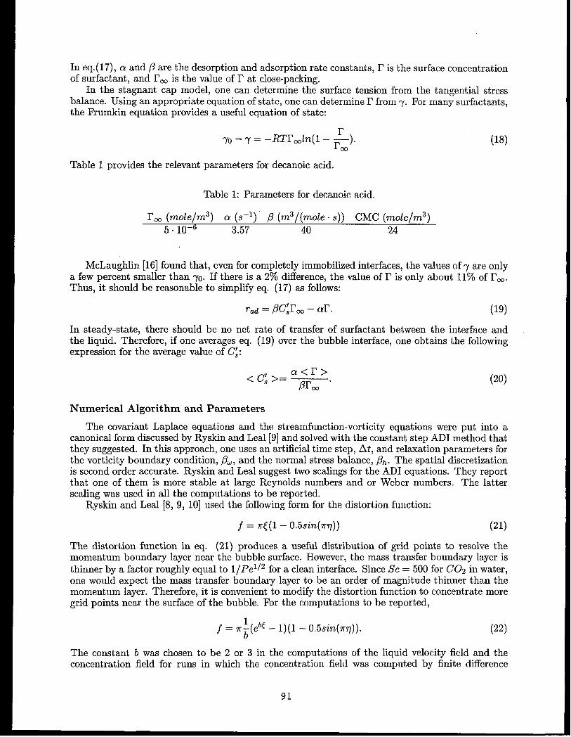
Table 1 provides the relevant parameters for decanoic acid.

Table 1: Parameters for decanoic acid.

17m (mole/nz3) a (s-l) /3 (m3/(nzoles s)) CMC (mde/nz3)5. 10-6 3.57 40 24

McLaughlin [16] found that, even for completely immobilized interfaces, the values of ~ are onlya few percent smaller than -yO.If there is a 2!Z0difference, the value of r is only about 1l% of 17m.Thus, it should be reasonable to simplify eq. (17) as follows:

Tad = Pc;rm – Cm. (19)

In steady-state, there should be no net rate of transfer of surfactant between the interface andthe liquid. Therefore, if one averages eq. (19) over the bubble interface, one obtains the followingexpression for the average value of C::

~<r>< c;’= /3rm “ (20)

Numerical Algorithm and Parameters

The covariant Laplace equations and the streamfunction-vorticity equations were put into acanonical form discussed by Ryskin and Leal [9] and solved with the constant step ADI method thatthey suggested. In this approach, one uses an artificial time step, At, and relaxation parameters forthe vorticity boundary condition, @u, and the normal stress balance, /3h. The spatial discretizationis second order accurate. Ryskin and Leal suggest two scalings for the ADI equations. They reportthat one of them is more stable at large Reynolds numbers and or Weber numbers. The latterscaling was used in all the computations to be reported.

Ryskin and Leal [8, 9, 10] used the following form for the distortion function:

j = 7r((l – oe5s~?l(7rq)) (21)

The distortion function in eq. (21) produces a useful distribution of grid points to resolve themomentum boundary layer near the bubble surface. However, the mass transfer boundary layer isthinner by a factor roughly equal to l/-Pel/2 for a clean interface. Since Sc = 500 for C02 in water,one would expect the mass transfer boundary layer to be an order of magnitude thinner than themomentum layer. Therefore, it is convenient to modify the distortion function to concentrate moregrid points near the surface of the bubble. For the computations to be reported,

f = n~(ebt – 1)(1 – 0.5sin(7r77)). (22)

The constant i5was chosen to be 2 or 3 in the computations of the liquid velocity field and theconcentration field for runs in which the concentration field was computed by finite difference

91

methods. It was found that this choice permitted a significant reduction in the total number ofgrid points in the ~ direction.

To compute the Reynolds and Weber numbers, an iterative procedure can be based on thefollowing equation:

w pvz—:= —Re2 yde “

(23)

Once one specifies the physical properties of the liquid and the size of the bubble, the ratio W/Re2is fixed. Thus, one can perform a run for values of W and Re that satisfy eq. (23) and determinethe value of the Morton number. If the Morton number differs significantly from the value forwater, one can select a second Reynolds number and compute the corresponding Weber numberfrom eq. (23). In practice, only a few iterations are needed to obtain conve;ged results.

FORMULATION OF MASS TRANSFER PROBLEM

The volume concentration of C02, c’, is assumed to vanish at infinite distance from the bubble,which is stationary in the frame of reference for which the computations are performed. The volumeconcentraticm at the surface of the bubble is denoted by c:. The concentration field is assumed toobey the folIowing PDE:

g+v”vc=;v%, (24)

where the c is the dimensionless concentration, which is defined by c = c’/~.It is useful to rewrite eq. (24) in terms of the orthogonal curvilinear coordinate system (~, q, +):

(25)

The finite difference solution of eq. (24) is similar to the solution of eqs. (6)-(7). McLaugh-lin [16] described the solution of the latter equations. The concentration field is computing by anADI time-stepping method:

1 azcn+lc~+l = cn + 1/2 + ——

hthq ~2q ‘

(26)

(27)

The operators in eqs (26) and (27) were discretized with central difference approximations atthe interior points of the &– q plane. Three point one-sided differences were used at the boundaries.

The surface flux and Sherwood number can be computed from the concentration profile.

RESULTS

Figure I shows the streamlines near a bubble. The equivalent spherical diameter of the bubbleis lnwn. The surfactant cap angle is 90°. The presence of a wake region beneath the bubble isevident. In the bubble’s frame of reference, the liquid velocity in the wake is small in magnitudecompared to the free stream velocity. Also, the liquid in the wake has a large residence time andone might expect much of it to be nearly saturated. For these reasons, as pointed out by Lochieland Calderbank [1] one might expect the wake region to contribute relatively little to the overallmass transfer rate. Later, this idea will be documented.

92

t“” ’” ”’” ’” ’’”i ’” ’’’””~

30

25

. 2.0

,,

,0

0.3

00

Figurel: Streamlines around the bub-ble for de = l. Omnz,# = 90°.

omenm 180-.0’20 ‘% ‘w

Figure 2: Concentration con-tours around the bubble ford, = l.Omm, ~ = 90°0

Figure 2 shows contours of the concentration field for the bubble in Fig. 1. The contoursare shown in dimensionless boundary layer coordinates (z’,y’), where d is measured from the topof the bubble and y’ is measured perpendicular to the bubble surface. At the leading edge ofthe surfactant cap, the concentration contours are pushed away from the bubble surface. Thisphenomenon is caused by the retardation of the tangential motion of the liquid by the surfactantcap that causes liquid to be pushed away from the bubble.

.

m -

403 -

Sh

Xa -

1m -

Im -

0 j0336090 ~lzoialm

Figure 3: Comparison of computed Figure 4: Surface flux.and theoretical Sherwood numbers.

Figure 3 shows the Sherwood number as a function of the cap angle for the three bubble sizesconsidered in this paper. It may be seen that the Sherwood number decreases almost monotonicallywith cap angle. The only deviations from monotonicity are probably due to numerical error. Someof the decrease is due to the immobilization of the interface and some of it is due to the formationof wake.

Figure 4 show the surface flux as a function of the polar angle for the bubble in Fig. 1. The fluxis significantly smaller in the immobilized portion of the interface than in the rest of the interface.The flux is still smaller in the wake region.

Figure 5 shows the ratio of the wake volume to the bubble volume as a function of the capangle for ee = O.7mm, 1.Omm, and 1.5mm. When the cap angle is smaller than a critical value,there is no wake. As the cap angle increases beyond the critical value, the wake volume increases

93

Figure 5: Ratio of the wake volume tothe volume of the bubble.

Figure 6: Contribution to the masstransfer by the wake.

rapidly and reaches a local maximum before decreasing to the value for complete immobilization.The phenomenon of a local maximum has been :noted by McLaughlin [16] and Cuenot et al. [17].On the clean portion of the surface, the tangential component of the velocity is nonzero. Whenthe liquid encounters the surfactant cap, it is pushed away from the surface of the bubble andthis appears to play a role in producing a larger wake than one would obtain with a completelyimmobilized surface.

Figure 6 shows the fractional contribution of the surface flux in the wake region to the Sherwoodnumber. Results are shown for all three bubble sizes considered in this paper. The results areplotted as a function of the cap angle.

It is of interest to relate the Sherwood number to the volume concentration of surfactant. Theconvective-diffusion equation for the volume concentration of surfactant was not solved in thisstudy. Therefore, it was not possible to obtain precise information about the dependence of theSherwood number on the bulk concentration of surfactant. However, one can use the approximationin eq. (20) to relate the Sherwood number to the average volume concentration of surfactant nearthe bubble surface.

‘,W

‘)M

:m-

:WSh

?W

m -

15-I-

ICC-

m-O,w O.cmo O,wm O.ca’a 0w O.ww 0cow o.c970

.m(m.kdr?]c’

Figure 7: Sherwood number depen-dence on Cj.

Figure 8: Comparison of Sherwoodnumber correlation with the com-puted values.

The surface tension even for completely contaminated interfaces differs by only a few percentfrom the VdUe for a clean surface. This justifies the use of eq. (20). Figure 7 shows the Sherwood

’94

number as a function of the average value of C:.

Correlation for the Sherwood number

For a bubble of diameter de, the Reynolds number, Rem, and Sherwood number, Sh~, for aclean bubble can be estimated from

Rem = –25.544 + 515.884de (28)

Sh~ = 2“96 l/2pelf2,LW – ~1 (29)

where de is measured in mm. The equation for Ren is a fitto the experimental data obtained byDuineveld [18] and is valid for 0.6 mm< d. <1.8 mm. The equation for the Sherwood number isthe analytical expression derived by Lochiel & Calderbank [1].

For the completely contaminated bubble

Reim = :[1 +Ar/96

(1+ 0.079ArO”TAg)OTss]-1(30)

Shim = 0.725Re~~Sc1i3, (31)

where Ar, the Archimedes number, is given by Ar = d~p2g/p2. The expression for Reim wasdeveloped by Anh Nguyen [19] and the equation for Shim is a modification of the expressionderived by Lochiel & Calderbank, with the multiplying constant decreased from 0.84 to 0.725 sothat it fits the computed data.

The value of the Sherwood number, Sh, of a bubble with diameter d, and Reynolds number Recan be calculated as follows:

Re – Rezmz

= Rem – Reim

Y = ~0”434Sh = y(Shm – Shim) + Shim

Figure 8 compares the computed values of Sh with those obtained using the correlation.

CONCLUSION

The main results of this paper are summarized below.

●

●

●

●

●

●

The Sherwood number, Sh, is strongly affected by the stagnant surfactant cap angle.

(32)

(33)

(34)

TheSherwood number is more strongly aff;cted by @ for-larger bu~bles in the size range considered.For cap angles smaller than about 50°, the stagnant cap has little effect on the Sherwoodnumber. For cap angles larger than 150°, Sh is approximately constant.For the largest bubbles, Lochiel & Calderbank’s estimate of the wake’s contribution to Sh isfairly close to the computed value, but their estimate is substantially larger than the computedvalue for the smaller bubbles.The results shown are for bubbles that have risen 15cm. If the bubble rose further, thecontribution by the wake would be smaller.Sh shows a monotonic decay with the subsurface concentration of surfactant. In all cases thesurface tension varies by less than 2 Yoaround the bubble.The quasisteady assumption for the bubble radius was justified by a computation of thedistance needed for the radius to decrease by 10%. However surfactant sorption kinetics mayintroduce a strong age dependence of Sh and thus require simulation of the unsteady bubblemotion.A correlation for Sh for bubbles in dilute aqueous solution of surfactant was presented.

95

ACKNOWLEDGEMENTS

This work wassupported bythe U.S. DepartmerIt of Energy under Grant DE-FG02-88ER13919.Some of the computations were performed at the National Energy Research Scientific Computing(NERSC) Center.

[1]

[2]

[3]

[4]

[5]

[6]

[7]

[8]

[9]

[10]

[11]

[12]

[13]

[14]

[151

[16]

[17]

[18]

[19]

REFERENCES

Lochiel: A.C. and Calderbank, P.H. (1964) Mass transfer in the continuum phase aroundaxisymmetric bodies of revolution. Chem. Eng. Sci. 19, 471-484.

Boussin.esq, J. (1905) Calcul du pouvoir refroidissant des courants fluids. J. Math. 6, 285-332.

Frossling, N. (1938) Uber die Verdunstung fallender Tropfen. Ger. Beit. Z. Geophysik 52170-216.

Griffith, R.M. (1960) Mass transfer from drops and bubbles. Chem. Eng. Sci. 12198-213.

Bowman, C.W., Ward, D.M., Johnson, A.I., and Trass, O. (1961) Mass transfer from fluid andsolid spheres at low Reynolds numbers. Canad. J. Chem. Engng. 399-13.

Friedlander, S.K. (1957) Mass and heat transfer to single spheres and cylinders at low Reynoldsnumbers. AIChE J. 3, 43-48.

Friedlander, S.K. (1961) A note on transport to spheres in Stokes flow. AIChE J. 7, 347-348.

Ryskin,, G. and Leal, L.G. (1983) Orthogonal mapping. J. Compui. Ph~s. 50, 71-100.

Ryskin, G. and Leal, L.G. (1984a) Numerical solutions of free-boundary problems in fluidmechanics. Part 1. The finite difference technique. J. Fluid Mech. 148, 1-17.

Ryskin, G. and Leal, L.G. (1984b) Numerical solutions of free-boundary problems in fluidmechanics. Part 2. Buoyancy-driven motion of a gas bubble through a quiescent liquid. J.Fluid AJech. 148, 19-35.

Duineveld, P.C. (1995) The rise velocity and shape of bubbles in pure water at high Reynoldsnumbers. J. Fluid Mech. 292, 325.

Haberman, W.L. and Morton, R.K. (1953) An experimental investigation of the drag andshape of air bubbles rising in various liquids. David Taylor Model Basin, Rep. no. 802.

Haberman, W .L. and Morton, R.K. (1954) f!m experimental study of bubbles moving in liquids.Proc. Am. Sot. Civ. Eng. 387, 227-252.

Saffman, P.G. (1956) On the rise of small air bubbles in water. J. FluidMech. 1, 249-275.

Hartunian, R.A. and Sears, W.R. (1957) On the instability of small gas bubbles moving uni-formly in various liquids. J. Fluid Mech. 3, 27-47.

McLaughlin, J.B. (1996) Numerical simulation of bubble motion in water. J. Colloid InterfaceSci. 184, 613-624.

Cuenot, B., Magnaudet, J., and Spennato, B. (1997) The effects of slightly soluble surfactantson the flow around a spherical bubble. J. Fluid Mech. 339, 25-53.

Duineveld, P.C. (1994) Ph.D. Dissertation, University of Twente.

Nguyen A.V. (1998) Prediction of bubble terminal velocities in contaminated water AIChEJournal 44226-230

~?6

MORE ON THE DRIFT FORCE

Graham B. Wallis

Thayer School of Engineering, Dartmouth CollegeHanover, NH 03755 U.S.A.

ABSTRACT

The previous theory for the drift force on an object in an inviscid weakly rotationalflow is supported by experimental” data, numerical CFD experiments, and additionaltheoretical derivations.

INTRODUCTION

The “drift force” was introduced at this symposium three years ago by Wallis (l). Simplifiedanalyses were presented to derive components of the force on a stationary object in a flow andwere shown to be consistent with the general expression

where U and u are the mean incident fluid velocity and (weak) vorticity, p the fluid density, V thevolume of the object and Q or Cj~ the added mass tensor for the object. The drift force resultsfrom the wrapping of vortex lines around the object, their stretching, trading and displacementin the object’s wake. Because vortices move with the fluid? these displacements may be relatedto the “drift” of fluid particles due to the presence of the object.

Wallis claimed that the drift force should be added to the “polarization force” resulting fromthe interaction between the velocity gradient in the oncoming flow and flux sources that areimagined to create the object. This polarization force is

FP=pV(U. VU+ U.~. VU) (3)

which, when added to (1), gives a net force of

F = pv(u oVU + V~U . ~ . U) or Fi = pV[Uj~Ui/8xj + 8/8x~(UjCjkUk/2)] (4), (5)

The present paper reports some results of three independent approaches to put these deriva-tions on a sounder basis:

a) Experiments in a wind tunnel.

b) Numerical experiments using the CFD package FLUENT.

c) More thorough and complete analytical derivations.

EXPERIMENTS

Rlfeetd. (2)measured thel.ift force on a set ofobjects (Figure l)placed ina wind tunnel(Figure 2) in which an approximately linear velocity gradient was setup by providing a suitably-varied flow resistante at the inlet to the tunnel. The lift force was measured for different values ofmean velocity U, at the axis of the object, and velocity gradient, dU/dy. Results were correlatedby determining the optimum coefficients, CL and B, in an equation of the form

FL = pVcLU~ + BU2 (6)

(>!-6t-

‘Sloued Plate~

Fig. 1: Cross-sectionof axisymmetric Fig. 2: An object in thewindtunnel.objectsusedin theexperiments.

B is constant for a given object and represents a small component of lift, due solely to theaverage flow, caused by small misalignments ancl asymmetries. The objects had a hemisphericalnose and various forms of streamlined tail designed to achieve a separation-free flow. This isdesirable in order to approximately duplicate a potential flow on which the theory depends. The“base” objects in each series are sketched in Figure 1. Larger objects with the same shapes butwit h volumes that were an integral multiple of the “base” volume were also tested.

The added mass coefficients were measured for these same objects by mounting them onsprings, suspending them in either air or water, and recording the natural frequencies of oscillationin each case (2). Comparisons between measured lift coefficients and added mass coefficientsshowed substantial agreement (Figure 3).

CFD SIMIJLATIONS

Song (3,4) used the commercial CFD package FLUENT-UNS to simulate Rife’s experiments.Besides giving predictions of the lift coefficients, these studies also revealed details of the flowstructure that generally support ed the mechanisms postulated in the theory.

Figure 4 shows the centerplane (z = O) streamlines for flow around the “base” bomb inlaminar shear flow. The stagnation point is lifted on the nose of the object, by the vorticitywhich girdles it, and there is a downwash in the wake which is symptomatic of the reaction ofthe lift force on the fluid. Very similar streamlines are obtained if turbulent flow is assumed. Thepressure distribution on the object reveals a region of low pressure on the top side, causing anupwards lift force. In the wake, looking at the object from behind, there are two major regionsof trailing vorticit y, causing a strong downvmsh. resembling what occurs behind a lifting surfacesuch as the wing of an airplane (Figure 5).

Table 1 summarizes the lift coefficients obtained from physical experiments (2), the pre-dictions of laminar or turbulent CFD models, and the corresponding experimentally-determinedadded mass coefficients. The predictions are quite good, though somewhat below the measure-ments. Laminar conditions (imposed in the CFD menu) generally lead to higher lift, perhapsbecause these conditions are closer to the theoretical assumption of inviscid flow (though theexperiment al conditions were turbulent). Varying the velocity gradient gave consistent values oflift coefficient. Attempts to use the RAMPANT code to model inviscid flow over these objectsyielded more scatter.

.~ V.a

L_-%+.,.~.b + CM,t.O.tI

j 0.2 + CL. mm * CM, COIIRI

fJ, % + CL, .aksMp ~ CM, airship

o024681012 ——.

—-

Flg.3: Lift coefficient,CL, in a“shear flow comparedwith Fig. 4: Streamlines in center plane of bombadded mass coefficient, CM, for the threeobjectsillustratedin 1 in laminar flow. p n 1.7894 x 10-5kq/ms,Fig. 1. p = 1.225kg/?l13

LiftCoefficientCLObj. vol. C,l.r

Exp. Turb. Lam.

1 0.3992 0.3147 0.3631 0.402

2 0.4278 0.3243 0.3471 0.397

Bomb 4 0.3559 0.3032 0.3199 0.381

8 0.3526 0.3268 0.3479 0.37816 0.38340.33890.3538 0.3961 0.29920.20800.2411 0.280

Comet 2 0.27600.20690.2223 0.2694 0.25300.23040.2469 0.2691 0.16130.14080.15920.158

Airship 2 0.13820.13540.1520 0.1494 0.12310.12310.1315 N/A

99

Table 1: Lift coefficientsobtainedfor all objectswith both Iaminarand turbulentconditions(p =1.225kg/m3and# = 1.7894x 10-5)

,,’1 ,;,

Fig, 5: y- and z-velocity components onz=370n~m plane. (bomb 1 in laminar flow.p = 1.7894 x 10-5kg/nzs, p = 1.225kg/m3)

According to the theory of vortex line drift, the axial (x-direction) vorticity in the wakeresults from wrapping, or “hanging-up”, of vortex lines around the object. The trailing axialvorticity can be used to derive the lift force in much the same way as the classical deduction oflift on an airplane wing. It is predicted that the moment of x-direction vorticity about the z – yplane through the middle of the object is

I dUzwzdydz = —CZZV

dy(7)

where CZZ is the principal component of the added mass tensor in the x-direction. This momentwas evaluated, from data like that appearing in Figure 6, and the equivalent coefficient Cm,replacing CZZ in (7), computed. For three objects, e.g., Table 2, Cm extrapolates closely to CZZat the y – z plane at the trailing edge of the object (approximately at the location correspondingto the first row in each table) and declines with distance from the object in the wake as vorticitydiffuses due to turbulent mixing and numerical diffusion.

Fig. 6: z-vorticity contours on z=450111mplane. Elomb 1 in turbulent flow with ill-let turbulence level of 1%, ancl ii = 4m/.s.8U/t@ = 20/s, p = 1.225kg/t773,p = I.is!l.t xlo-skg/???.$.

THEORY

x Left Right Sum Derived

(mm) x 10-’ XlO-’ i 10-’ c&f

1400 I 1.341 1.391 I 2.732 0.2899

410 1.335 1.362 2.696 0.2860

420 1.104 1.371 2.476 0.2627

430 1.272 1.115 2.387 0.2533

440 0.907 1.215 2.121 0.2233450 0.901 1.226 2.126 0.2238

Table2: Integralof vorticitymomentin thewake.Cometin laminarflowwithii = 4m/s,8u]8.v= 20/s,p = 1.225kg/m3,p = 1.7894x10-5kg/m s. CM: 0.280

The theory has evolved considerably since its initial formulation (1). Several examples willbe given:

Example I. The earlier momentum balance for a box surrounding the object did not account forthe displacement of streamlines out of the sides of the box (Figure 7). A fluid particle, or vortexline, that is located on the straight side of the box has been displaced an amount b by the presenceof the object. The amount of z-direction vortick y lost from the rectangular box on the top andbottom is then u, j bvdsy because bv is small. Since this reduces J tizdV in the previous equation(13) it appears that (14) in the 1995 paper should read

(8)

.) Vortex lines. originally i. lIK zdkwdrm. strckkd amoti a. objeu b) Smtion in a z-pi=. sh+wingdkeui.m of secondaryflow cornpawntsat Iw.ndarks dw to rnmicity entrainedin k wake and IOSLon zhesidesof k Ccnlml volume

Fig. 7: Control volume for Lighthill’s problem.

Now Bernoulli’s equation of the 1995 paper expressed the pressure perturbation solely interms of the perturbation in pv2/2, ignoring the fact that the stagnation pressure has also beenperturbed because the streamline through the side of the box is not the same one that wouldbe there in the unperturbed flow without the object. From Crocco’s Equation the perturbationin stagnation pressure is –pb oU x u, so for U in the x-direction and w in the z-direction, thepertur~ation in pressure from both the influences is

when (9) is used in (8) the drift force in the y-direction isto be

The two effects that were previously neglect ed balanceno influence on the drift force.

(9)

again computed, as in Wallis (1995),

(lo)

each other exactly and together have

Example II. The sideways drift that was previously sketched qualitatively has now been computedfor discs and ellipsoids at various angles of attack. A typical result is presented in Figure (8).It shows a network of fluid particles that were introduced to form a uniform mesh in the region(–1 < y < 1), (–1 < z < O) at z = –10. These particles flow over a circular disc of unit radiuswith its center at the origin and tilted at 45° to the y-axis. At the time when these particleswould reach z = 10 if there were no disc? their positions are shown in Figure (8). Their y- andz-coordinates are almost exactly the same as they are when the same particles cross the planex = 10. They represent permanent transverse displacements of streamlines in the wake.

The 3-O We Iiie fw tiomn flow P* a dk al pi/4,.

:/........ . .

-1.51-1.5 -* -0.s o 0.5

z

Fig. 8: Transversedrift in the wakeof a tilted disc.

Displacements are generally downwards over the area indicated, inwards for positive y andoutwards for negative y. The streamlines near those passing through the stagnation points aredifficult to resolve, requiring a finer grid and more accurate computation.

These results have enabled us to compute and check several integrals in a general theory ofdrift (too extensive to present here) that also appear in a more general theory for the drift force,using a control volume of any shape. A few loose ends remain to be tied up.

Example 111 At the 1995 Symposium (1) a “polarization force” was derived for an object in apotential flow with a velocity gradient. It was computed to be

FP=–pD. VU=pV(”UOVU+UQVU) (11)

where D is the polarization, or dipole moment of flux sources used to represent the object.

When the flow is not potential, the forces on. the object result from interactions between theflow and both flux and circulation sources, the latter including the vortex lines that wrap aroundthe object. The flux sources of strength pm per unit volume at location rj with dipole moment

II

Dj = rjp~dV (12)

produce a velocity which is minus the

The component of the force that

gradient of a potential

8#du~k=–—

hk(13)

is due only to the interaction between these flux sourcesand the unperturbed flow is evaluated from a large control volume around the object:

/(

8Uk aui b’uk‘—udkds~ – Tj ‘- UdkdSk – ‘rj

‘J Ozj 8X j—Ud~dSk8Xj )

(14)

The surface integrals may be evaluated by converting to volume integrals and treating theflux sources as distributed. The factor of t3Ui/i?x j is

J

~j~dsk=/&(Tj$)dv

=

I( %+ T%9dv=N$-IYPm)dv= J~ddSVD~

(15)

and the factor of 8Uk/6’xj is

Therefore, (14) may be expressed as

(16)

(17)

1102

The first term in (17) leads to the “polarization force” obtained earlier in (11). The second termvanishes in an incompressible flow. The final term is proportional to the vorticity and to a surfaceintegral that depends on the choice of control volume. Since the net force is independent of such achoice, there must be a compensating term from other components of the force, involving particleand vortex line displacements due to “drift”.

Example IV. An alternative representation of the object is by circulation sources wrapped aroundits surface to account for the velocity jump between the solid and the surrounding fluid. Considerone of these vortex loops of strength dI’ described by the vector location r (or ?’k)of points alongit. The “lift force” on an element of this ring due to interaction with the unperturbed flow mightbe expected to be

dF = P(U + r ~VU)xdrdr (18)

When this is integrated along the entire ring the first term on the right hand side vanishes because~ dr = O. The remaining term, in index notation, is

(19)

and the z-component is explicitly

Now, for integration around the entire vortex loop we have

I’d%= /@y= Izdz=o /@@+@x)= Id(xy)=o (21),(22)J J J

and hence

;/xdy = – ydx

with similar expressions in the other directions.

Also, by definition

J

I; (zdy - ydx)=— (23)

(24), (25)

Using (21) through (25) in (20) we obtain

2dF’

\ ( )/ ( 3—= (zdy- y(k) W-g + (zdy-ydz) w,+pdr

I ( %)+ (zdx – zdz) Wz –

which is the z-component of

/VOV rxdr+wx

Ir x ‘r-(Jr x ‘bT

(26)

(27)

Now, Cai and Wallis (6) showed that the dipole moment of a stationary object in a flow can beexpressed as

D=;/

rxdrdr (28)

and therefore (19) integrated over the entire object yields

:=(V. V)D+U X D- D*VU (29)

The first term vanishes in an incompressible fluid. The second term may be expanded (6),

D= .Q. uv=-p+g. uv (30)

to give the drift force pVU “~ x w together with an additional term pVU x w that wouldresult if the object “froze” the unperturbed vorticity threading it. This might be justified by theargument that the representation of the object by vortex rings does indeed reduce the velocityinside it to zero, whereas the “model” using flux sources sweeps the ends of the internal vortexrings to the rear stagnation point whence they stretch along a long filament to join their remaininglengths far in the wake. The final term is the polarization force in (11) that also appeared in (17).

The pcint of examples III and IV is that partial superpositions yield some of the desiredforces and axe only consistent when there is no vorticity in the main flow. A complete formulationshould consider the effect of the displacement of the external vortex lines as well.

1.

2.

3.

4.

5.

6.

REFERENCES

G.B. WALLIS, “The Drift Force on an Object in an Inviscid Weakly-Varying RotationalFlow,” Presented at the Thirteenth Symposium on Energy Engineering Sciences, ArgonneNational Laboratory, May (1995).

J. RIFE, J. HE, Y. SONG, and G.B. WA.LLIS, “Measurements of the Drift Force,” Nut.Eng. Design, 175,71-76 (1997).

Y. SONG, “Numerical Study of Drift Force (onObjects in Sheared Flow,” M.S. Thesis, ThayerSchool of Engineering, Dartmouth ColIege, March (1998).

Y. SONG and G.B. WALLIS, “Numerical Study of Drift Force on Objects in a ShearFlow,” Presented at the Third International. Conference on Multiphase Flow, ICMF’98, Lyon,France, June 8-12 (1998).

G.B. WALLIS, “Polarization of an Object in a Potential Flow: Some Theorems and Applica-tions to Ellipsoids,” Advances in Multiphase Flow, Eds. A. Serizawa, T. Fukano, J. Bataille,Elsevier Science B.V., 185-189 (1995).

X. CA.I and G.B. WALLIS, “The Added Mass Coefficient for Rows and Arrays of SpheresOscillating Along the Axes of Tubes,” physics of ~hi(k A, 5(7), 1614-1629 (1993). -

1.04

SIMULTANEOUS SMALL ANGLE NEUTRON SCATl_TWNG AND RHEOMETRIC

MEASUREMENTS ON A DENSE COLLOIDAL SILICA GEL

Howard J.M. Hanley, Chris D. Muzny and Brent D. Butler

Physical and Chemical Properties Division,

National Institute of Standards and Technology’,

Boulder, CO 80303

ABSTRACT

Small angle neutron scattering (SANS) intensities, from a dense (volume fraction

O.17) colloidal 7 nm silica gel, were measured as a function of the scattering wave

vector and of time for systems gelled statically and gelled in the presence of an

applied constant strain rate. The viscometric behavior of the system was measured

simultaneously. The substantial differences between the structure of the gel formed

statically and under shear are discussed. The effective hydrodynamic diameters of

the aggregated components of the gel were estimated by dynamic light scattering.

INTRODUCTION

We present small angle neutron scattering (SANS) data from a dense solution of colloidal

silica gelling under an applied shear rate. The key data are the time dependence of the scattered

intensity l(q, t) as a function of the wave vector q (where for neutrons of incident wave length a,

q = (4@sin(efl) with 0 the angle between the incident and scattered neutron beams) and the

corresponding shear viscosity q, and shear stress r. This is a pioneering experiment. Our interest

here is to see how shear affects the gelation mechanism and the structure of the final gel, but the

procedure has wider implications. For the first time, it is possible to measure SANS structural and

‘Publicationof the National Instituteof Standardsand Technology,not subject to copyrightin the USA.

viscometric data simultaneously because we have recently adapted a commercial constant stress

rheometer tcl couple with the 30 m SANS spectrometers at the NIST Cold Neutron Research

Facility (NCNR) [1].

2D Detector (in XZ- plane)

Y

Scattered Neutrons

~ .5

&

INeutron beam

Figure 1. Beam path through the rheometer modified for SANS experiments.

Figure 1 shows schematically the beam path through the instrument which is setup in a

Couette shearing mode with the sample (volume approximately 7 ml) contained in the annular gap

between an inner cylinder (rotor) and a stationary outer cup (stator). The gap width is set at

0.5 mm or ‘1mm by the appropriate choice of a rotor-stator pair. For these experiments, the beam

was incident along the y–axis and the scattered intensity recorded on a SANS two-dimensional

detector placed in the xz–plane. Scattering from a gelling silica sample was measured with the

system at rest, and when subjected to a constant applied shear rate,y = du~dy. Here, the flow

velocity of the sample is in the x–direction, UX. The rheometer operations and SANS output are

linked and synchronized through a personal computer.

SAMPLE PREPARATION AND SANS SET-UP

All the experiments were carried out on gels made from a common stock of commercial

grade Ludox SM-30 [2] – a stable aqueous colloidal silica suspension at pH = 9.8. The silica

spheres were designated by the manufacturer to have a nominal diameter o = 7 nm with an

estimated 20% polydispersity. We determined the suspensions were 31% by mass SiOz

(corresponding to a volume fraction@ = O.17) with a suspension density p = 1.215 g“cm-s.

Sols were prepared by filtering the suspension through 0.45 ym membrane filters.

Concentrated HC1 was added to the sol until the pH was lowered sufficiently to initiate gelation.

For convenience, we required that the time scale of our SANS experiments was such that the gel

point was about 60-90 min after initiation, and that a final gel formed after about 8 h. Hence, for a

typical experiment, 140 A 3 pl of concentrated HC1 (12 mol. din-q, p = 1.186 g“cm-q) were added

to 12.15 g of the filtered sol (10 ems), and the resulting mixture was vigorously agitated for

about 30 s. The initial pH of the gelling mixture was measured to be 8.02 A 0.02 and was found

not to change noticeably during the gelation process.

The SANS experiments were carried out on the 30 m SANS NG7 spectrometer configured

with an incident neutron wavelength k = 0.7 nm and a sample-detector distance of 13.6 m with a

0.25 m offset, giving a wave vector range of 0.03 c q (rim-1) e 1.2. The scattered neutrons were

detected on the instrument’s 2D position sensitive detector and the scattered intensities, l(q,t)

measured as a function of time t. We detected no anisotropy in the scattered intensity pattern, so

the measured counts were azimuthally averaged and these averaged intensities were corrected for

empty cell and solvent scattering in the usual way and placed on an absolute scale by normalizing

to the intensity of a water standard [3].

After gel initiation the sample was placed immediately into the Couette cell of the modified

rheometer. After loading, the rheometer was set to apply a constant applied shear rate, and the

SANS intensities and viscometric data, specifically the shear viscosity, recorded as a function of

time. The counting intervals were selected to be consistent with the viscosity variation of the

gelling sample. Data were collected and averaged over 5 min intervals at times up to and just

beyond the gel point, and collected and averaged at 20-30 min intervals for, at least, another 4 h,

or until the scattered intensities became essentially time-independent. Thermostatting was ambient

at 25 & 2 ‘C. Some data were recorded with the rheometer in constant stress mode, but the

majority of data were taken when the sample was subjected to a constant shear rate of 244 s-~,

533 s-l and 1645 s-l with a Couette cell gap width of 0.5 mm. Additional runs with a cell gap

width of 1 mm were carried out on selected samples.

30

25

‘g 20

15

10

5

1 0 solx gel, 5 min I 1

0 ~~

o 0.05 0.1 0.15 0.2 0.25 0.3 0.35 0.4

q, rim-l

Figure 2: SANS intensity curves showing the time variation of the static colloidal silica gelling

system compared with curve for the SOL

Figure 2 shows three curves of the scattered intensity from the static (that is, non-sheared)

system as a function of time: at zero time when the system is the precursor suspension or sol, and

at 5 min and 4 h after gel initiation. The rise in intensity for the sol near q = 0.4 nm- 1 results from

scattering between the sol particles (spaced about 16 nm apart). At very early times after gel

initiation, this particle-particle separation peak disappears because the addition of HC1 increases the

screening of the charged colloidal spheres, hence decreasing their effective interaction diameter and

the effective volume fraction of the particles. Also, shortly after gel initiation, a less intense peak

appears at hligher q (-O. 8 nm- 1, not shown in the figure) which represents particle-particle contact

at about 7 nm.

The onset of the clustering that characterizes the gelled state is represented by the rise in

scattering power at low q. As time progresses the low-q scattering continues to increase indicating

coarsening of the clusters. At later times a peak in this low angle scattering (shown here at

108

approximately q = 0.2 rim-l after 4 h) can be identified and its location can be used as a rough

measure of the cluster-cluster correlation distance; -20 nm.

As observed previously, the low-q scattering is substantially enhanced in a system under

shear [4]. Figure 3 displays the scattered intensity from the gel at 4 h after gelation when the

109

system was subjected to a constant shear rate ~ = 533 s-1. For times longer than 4 h, the intensity

at low q increases slowly with time until it remains essentially static after 8 h. It is important to

note that this long-time intensity curve does not change noticeably after the shear is turned off.

Similar results were obtained from the gel at other shear rates.

140 , I I I I 1 I I 1 1 i 1 , I I 1

●I I I

120 :

y 100 - ‘o m:g

80 ~ ●

& ●

“~ 60 :●

●

ii 40

20 :

0 1 1 4 I I 1 ? t 1 I ! , I I I t ! I 1

0 0.05 0.1 0.15 0.2q, nrn-l

Figure 3: SANS intensity curve from the system 4 h after gel initiation compared with the curve

from the system gelled statically.

We now examine the juxtaposition of the time-dependent scattered intensities measured

from the sheared system with the behavior of the viscosity measured simultaneously. If the

system is subjected to a low constant shear stress, and then gelation is initiated, the viscosity will

increase until, at a time designated the gel point time, the viscosity becomes that of the solid. If,

instead, the system is subjected from initiation to a constant shear rate the viscosity peaks at a time

roughly equal to the gel time of an unsheared gel, but then the viscosity falls to an asymptotic

value that is higher than that of the initial sol but much lower than the peak viscosity. The state of

the sol at this asymptotic time is not that of a ‘broken’ gel, or a gel that has separated from

the container walls due to the high shear stress near the gelpoint (as one might suspect), but,

rather is that of a bulk fluid whose viscoelastic properties have been somehow altered by the

application of a shear. Figure 4 shows the viscosity/intensity time variation for the gelling

system subjected to a shear of 533 s-1 at q = 0.048 rim-l. Note; (a) the correlation between the

maximum in the viscosity and a jump in I(q, t) and (b) the increase in l(q, t) with t (to reach a

plateau value at long time) yet the system is liquid-like.

().8

0.7

0.6

(),5

0.4

(),3

().2

().1

o

1 1 1 I I I I 1 1 1 [ I 1 1 i 1 1 I 1 ! 1 1 I I 1 1 1 1 [I

1 I I 1 1

100

20

~~

o 60 120 180 240 300 36:Time, min

Figure4. ~Jariation of theviscosity coefficient with time forthesystem subjected to a constant

shear rate of 533 s-1. Superimposed is the scattered intensity measured as a function of time at

q = 0.048 rim-l. Both the viscosity and intensity were measured simultaneously.

Patterns similar to Figure 4 were seen fo:r systems subjected to other shear rates. We will

state here, and discuss in a future paper, the observation that in each case, although the peak

viscosities were different, the shear stresses on the sol at the peaks were nearly identical. A critical

stress value is thus likely an important parameter for describing gelation under shear.

Hvdrodvnamic diameters. An understanding and interpretation of the behavior of the scattering is

a subject of an ongoing investigation and further results will be discussed later. We, however,

wished to determine if the dramatic change in 1(’q,t),at times corresponding to the gel point time

results primarily from the growing size of the clusters or from a sudden change in the cluster

ordering. ,4ccordingly, for selected gelation runs, samples of the system were extracted and

diluted at va~rious times after gel initiation and the diluted samples were investigated by SANS and

by dynamic light scattering. About 0.05 ml of the gelling system was extracted from the Couette

cell at various times after gel initiation and added to 10 ml of deionized water. The diluted sample

was sealed in conventional cells and the dynamic light scattering correlation function and the

SANS intensities were measured; the hydrodynamic size and a Guinier radius of gyration of the

clusters could thus be determined. For the shear(ed system, we found that the diameters were close

to the equivalent diameters of the static gel for times up to the gel point, but then they increase

dramatically by about a factor of 30. This sharp increase in diameter corresponded with the

111

discontinuity in the intensity - and hence with the viscosity maximum and critical stress. Thus, it

is clear that the sharp rise in intensity near the peak value results primarily from a sudden change in

the cluster size, not from ordering. An additional interesting observation is that the aggregated

particles in these diluted samples decomposed in a few days until their sizes became roughly equal

to the particle diameters found in the initial sol – an unexpected result that indicates that the

aggregation of colloidal silica is reversible.

CONCLUSIONS

The objective of this short paper is to report on the data only; interpretation is minimal and

a more complete discussion will be forthcoming. We conclude, therefore, by highlighting some of

the results obtained:

1.

2.

3.

4.

5.

6.

Substantial differences in the low q behavior of I(q, t) are observed between gels formed

statically and gels formed under a constant shear rate. In general, I(q, t) increases at low wave

vectors as the gelation reaction proceeds, but, the increase is enhanced substantially when

gelation occurs in the presence of an applied shear.

Under static conditions, the shear viscosity increases as a function of time after gel initiation

and then diverges when the gel becomes solid. By contrast, under a constant shear, the

gelling system’s viscosity increases initially, but, after a time corresponding to the gel point

time, the viscosity decreases to an asymptotic value that is higher than that of the initial sol but

lower than the peak value.

At different shear rates, the viscosity at the peak is different, but, the shear stress at the peak

is approximately independent of shear rate. A critical shear stress is thus observed.

The time at which the critical stress, and the equivalent viscosity maximum, is reached

corresponds to a substantial and discontinuous enhancement in the low-q scattering.

Throughout the shear-influenced gelation, the system remains liquid-like in that it flows. On

removing the shear, the viscosity increases with time and the gel sets to a solid, yet the

structure of the material, measured by the SANS intensity patterns, does not change during

this setting process.

Samples from the system were extracted at various times after gel initiation. Dilute aqueous

solutions of the extracts were prepared, and characteristic effective particle diameters were

estimated by SANS and by dynamic light scattering. We found that the diameter increased

dramatically at a time corresponding to the jump in the scattered intensity. The isolated

particles formed under shear, however, they decomposed into units of size equal to the

particle size found at gel initiation, leading one to surmise that a colloidal silica gel is

reversible.

Finally, weremwk onthetechnological implications of theresults presented here. As far

as we are aware, it was not previously known that a silica sol, which has had its pH altered so as

to initiate gelation, could be held indefinitely in the fluid state by the application of a constant

shear. Apparently, there are no irreversible chemical reactions that prevents the normal formation

of a gel once this shear is removed. This implies that production of materials using the sol-gel

process might be accomplished via a continuous casting process instead of the currently used batch

process mocle. Such shifts in technology in other materials industries (steel, for example) have

reduced manufacturing costs markedly. It is, therefore, important to understand the structural

changes that. take place in the asymptotic regime of Fig. 4 that may impact a gel made from this

pre-sheared sol. Investigation along these lines continues.

1.

2.

3.

4,

ACKNOWLIEDGEMENT

This work was supported by a grant from the Division of Engineering and

Geosciences, Office of Basic Energy Sciences, U.S. Department of Energy. The

comments of John Bartlett and Elizabeth Drabarek of the Australian Nuclear

Science and Technology Organisation are much appreciated.

REFERENCES

G.C. STRATY, C.D. MUZNY, B.D. BUTLER, M.Y. LIN, T. SLAWECKI, C.J.

GLINK.A and H.J.M. HANLEY, “A Rheornetric Shearing Apparatus at the NIST Center for

Neutron Research (NCNR),” Nucl. Instr. and Methods in Phy.s. Res. (in press).

The tralde name is noted to identify the :product. Use of this material does not imply

endorsement by NIST.

C.J. GLINKA, J.G. BARKER, B. HAMMOUDA, S. KRUEGER, J.J. MOYER and W. J.

ORTS, “The 30 m Small-Angle Neutron Scattering Instruments at the National Institute of

Standards and Technology,” J. Appl. Crjst. ~ (in press).

C.D. MUZNY, G.C. STRATY and H.J.M. HANLEY, “Small Angle Neutron Scattering

Study (ofDense Sheared Silica Gels,” Phys, Rev.E ~ 675 (1994).

1:12

TURBULENT TRANSPORT PROCESSESINTERFACES

V. De Angelis and S. Banerjee

ACROSS

Department of Chemical EngineeringUniversity of California Santa Barbara

Santa Barbara, California

ABSTRACT

Experimental and numerical investigations of turbulent structure near the interface betweentwo flowing streams indicate qualitative similarity to those in wall turbulence – if the shear ratescorrespond. There are detailed differences, which depend on the interracial tension, fluid densitiesand viscosities for the gas and liquid streams. At atmospheric conditions, and restricting con-sideration to the wave scales important for scalar transfer (capillary waves), the differences areprimarily on the liquid side. The liquid-side tangential turbulent fluctuations peak right at theinterface, whereas on the gas side they peak a small distance away – much like in wall turbulence.In some sense, the liquid therefore sees the interface much like a slip surface, whereas the gas seesit much like a wavy solid wall. Furthermore, the patterns of shear stresses and pressure are pri-marily controlled by the quasi-streamwise vertical structures on the gas-side, with their associatedsweeps and ejections. Quasi-streamwise vortices also arise near the interface on the liquid side,but the associated sweeps and ejections do not correlate with the interracial shear stress pattern.Low-speed-high speed streaky regions are also seen near the interface on both sides, with theirspanwise spacing scaling with kinematic viscosity and friction velocity (defined for each side asthe square root of the ratio between the interracial shear stress and the fluid density). Ejectionand sweep frequencies also scale with the same parameters.

Turning now to heat and mass transfer mechanisms, they are primarily controlled by the sweeps,with ejections playing an important role in a certain range of Schmidt numbers on the gas side. Anunderstanding of the dominant mechanisms allows a simple parametrization of the scalar transfervelocity on each side, which compares well with experiments and direct numerical simulations.Capillary waves appear to have little effect on the parametrizations for scalar transfer velocity.

INTRODUCTION

Turbulence structure at boundaries govern high Reynolds number transport processes and mustbe elucidated for applications in the process and power industry, as well as in several atmosphericand environmental problems. A number of investigations have dealt with the phenomena thatoccur near solid boundaries. Work by Kline et al[l] and many others have shown that streaks oflow-speed/high-speed fluid form near the wall, and that these break down periodically in a spec-tacular phenomenon called a “burst”, in which fluid is ejected from the wall layer with significantwall-normal velocities. These “ejections”, and the associated “sweeps” that follow account fornearly 80% of the Reynolds stresses observed in boundary layers. Typical spanwise spacing of thestreaks are ~$ N 100, where A; is the non-dimensional spanwise spacing – the non dimension-alizing variables being the shear velocity, U7W= - and the kinematic viscosity, v. Rashidiand Banerjee [2], amongst others, have shown that, at sufficiently high Reynolds number, innervariables give a non-dimensional time between bursts T7W= (u~W/v)~W N 90.

113

In contrast to this understanding of the main features of turbulence near solid boundaries,albeit with many outstanding questions regarding the reasons for the phenomena, very little wasknown about turbulence near fluid-fluid boundaries till recently. This, in spite of the importanceof near-interface phenomena in determining mass and heat transfer rates in a variety of contactingequipment like gas absorbers and condensers, as well in geophysical problems like gas transfer atthe air-sea interface.

We do know that at fluid-fluid interfaces the mass transfer coefficient, ~, varies as the 1/2 powerof the molecular diffusivity, D, whereas at solid boundaries@ varies roughly as the 2/3 power of D.Obviously molecular effects are more important at solid boundaries, where turbulence is dampedmore than it is near clean, mobile interfaces.

The present study complements earlier experimental work by Rashidi and Banerjee[2] and isaimed toward a better understanding of such phenomena via direct numerical simulation (DNS),i.e. solving the full time-dependent 3-D Navier-Stokes equations without any closure model. ThisDNS aims to calculate the mean statistical properties of turbulence on both sides of the near-interface region, clarify mechanisms related to the coupling fluxes between the phases, with par-ticular regard to the role of turbulence structures (i.e. their appearance and evolution in theimmediate neighborhood of the fluid-fluid interface) and to develop scalar transfer parametriza-tion based on the physical insight gained from the DNS.

It can be shown that scalar transfer occurs over scales that are at most affected by capillarywaves. It therefore becomes possible to examine the controlling processes by DNS over a domainsize of the order of. several capillary waves, and in isolation from surface deformations that arelarger in scale.

freeslipA

171shearunits

171shearunits

v

GAS I1

( I LIQUID

freeslip

Figure 1: Geometry of the SimulationFigure 2: Bursts_from the liquid surfacecounter-current flow

for

The typical flow geometry, investigated as a canonical problem is shown in Figure 1. Gas flowsco- or counter-current to the liquid flow. The interface for moderate wind speed, NO (3-6 m/s),forms capillary waves that have amplitude of roughly a millimeter. Before discussing the effect ofwaves, however, we examine the turbulence structures on the liquid and gas side in the simplersituation in which the interface is kept flat.

2. GAS-LIQUID FLOW ACROSS FLAT GAS-LIQUID INTERFACES

Consider :now experimental conditions set to keep the liquid Froude number low and the gasvelocity low enough to be well away from Kelvin-Helmhotz instabilities. A non-wavy surface canbe obtained even when quite high shear rates are imposed, as shown by Rashidi and Banerjee[2].

They visualize the liquid side flow, using a lmicrobubble tracer technique, in a situation inwhich there is a wall at the bottom of the liquid stream. The high-speed, low-speed streaks seenby many investigators are found near the wall. However similar structures are also seen at highenough shear rates at the interface – whereas at low shear rate the interface structure looks patchy.Clearly there is a shear rate at which transitiomloccurs, but once streaks are established in thenear interface region, the similarity between the bursts seen in the vicinity of the wall and of theinterface is remarkable. This is shown in Figure 2, representing a side view of the liquid stream,with gas on the top going counter-current to the liquid.

114

Quantitative similarities were also found by Rashidi and Banerjee[2]. If the interracial streakspacing is non-dimensionalized with the interracial shear rate, then A; w 100j where A; = ~l’Ur~/U.Thus the interracial streak spacing scales in the same way as the wall streak spacing, providedone uses the interracial shear stress to obtain the velocity scale. Furthermore the period betweenbursts is seen to scale in the same way as at the wall, i.e. ~~1 ~ 90.

Even if the qualitative picture seems the same at a sheared interface and at a solid boundary,there are detailed differences between the two cases that will play a role in mass and heat transferprocesses.

Lombardi et al.[3] did a simulation assuming a flat interface. They resolved about 170 shear-based units, h+, on each side of the interface, where h+ is based on the interracial shear velocity,u~~.

Runs at different density ratios (R2) between the fluids were performed. The gas and liquidwere coupled through continuity of velocity and stress boundary conditions at the interface.

The interracial plane itself showed regions of high shear stress and low shear stress, with lowshear stress regions corresponding to the low speed regions and the high shear stress to the highspeed regions. The low shear stress regions are streaky in nature with high shear stress islands.At the edges of the high shear stress regions, vortices are seen to spin up on both sides of theinterface. These are initially in the plane normal to the interface but subsequently are stretchedin the quasi-streamwise direction by the mean flow. These quasi-streamwise vortices are knownto play a major role in the ejection-sweep processes observed in wall turbulence, and they do thesame at the gas-liquid interface.

0.070,

0.C40 “.0 nod0“ ❑+

o ..-0.0s0- *.-

0 ●IV00

0.040-000“0.. “o

. 0° “o0.030- .

. 0

:&0.0 20.0 40.0 60.0 80.0

interracial&carxlIY.3

0.070,

Figure 3: Probability of strongly coherent events classes accordingto quadrant as a function of interracial shear stress in theregion over which the events occur. left: gas; right: liquid

At this point it is worth considering how the high shear stress regions form. This can beclarified by considering a quadrant analysis of the velocity field over the interface in which velocityfluctuations in each quadrant of the Reynolds stresses are correlated with shear stress at theinterface. In the first quadrant both the streamwise and interface normal velocity fluctuations arepositive. In the second, the streamwise component is negative but the interface normal componentis positive. This corresponds to an ejection of low speed fluid. In the third quadrant both thestreamwise and the interface-normal velocity fluctuations are negative, and in the fourth thestreamwise component is positive whereas the interface-normal component is negative. The fourthquadrant then corresponds to a sweep in which high-speed fluid is brought towards the interface.Consider now the correlation of each quadrant of such velocity fluctuations with the interracialshear stress shown in Figure 3 (left) on the gas side. It is clear that sweeps, i.e., in the fourthquadrant, lead to the high shear stress regions whereas ejections lead to the low shear stressregions. This is what is observed in wall turbulence at a solid boundary and therefore the gas seesthe liquid surface much like a solid boundary.

However, if we look at Figure 3 (right), it is immediately clear that no such correlation existson the liquid side. In fact, all the quadrants have similar behavior with regard to the shear stressregions that occur below the high speed sweeps on the gas side, i.e. , the motions that bring highspeed fluid from the outer regions to the interface on the gas side, lead to the high shear stress

115

at the interface. Conversely, ejections on the gas side which take low speed fluid away from theinterface into the outer flow, strongly correlate with low shear stress regions. The liquid does notbehave in this way and does not dominate the pattern of shear stress on the interface.

(b=l ..%..0.0~

. J

0.0 40.0 80.0 120.0 la.”z’

3.0

; 2.0,.>E.~B

-------..

‘.

0.0 m“ 80.0 120.0 la.”z“

Fi ure 4: Results from direct numerical simulation on rmsfve ocity fluctuations, left: gas; right: liquid

The difference between the gas and the liquid phases in the near interface region is furtherclarified by observing the velocity fluctuations on each side of the interface as shown in Figure 4.The left portion of the figure is for the gas whereas the right figure is for the liquid. The gas, as isevident, behaves much like flow over a solid wall. The fluctuations are almost identical to that ata solid boundary, in all directions – streamwise, spanwise, and wail-normal. On the other hand,the liquid, as evident from the figure, has the largest fluctuations in the streamwise and spanwisedirections right at the interface itself. It sees the interface virtually as a free slip boundary, exceptfor the mean shear. As a consequence, vertical fluctuations vary as the first power of normaldistance, and the square of the normal distance, on the liquid and gas sides, respectively.

These observations are of some importance for the scalar flux on the gas and liquid sides. Themass transfer velocity ~+ is defined as: ~+ = - 1 ~ ,where ~ is the nondimensional

\fi~SC(Co-C~) dxs

gradient at the interface and cb and COare the bu]k and interface concentrations. Mass transfertakes place at the interface by conduction only, therefore it is enhanced when bulk fluid is conveyedto the interface region, e.g. by sweeps. We extencl the quadrant analysis and look at the correlationof the Reynolds stress – and therefore of the turbulence structure, in the various quadrants withthe instantaneous value of mass transfer velocity fl+ at the interface.

Results are reported in Figure 5 for Sc=l and SC=1OOon the gas side and liquid sides. In allthe cases, except for SC=1OOon the gas side, IV (quadrant events (sweeps) are seen to generate thehighest values of the mass transfer velocity. This is evident when looking at the probability of suchan event to occur (fP) and at the fraction of the total flux through the interface associated with it(~~), as in Table I. On the liquid side the sweeps carry a larger fraction of mass flux (N 0.50), thantheir probability (~ 0.30). On the liquid side the interface can be efficiently renewed by sweeps,because the horizontal fluctuations are unimpeded. On the gas side the situation in modified bythe different boundary conditions. At low Sc number, sweeps and Quadrant I events are seento be the most efficient for scalar transfer, but when the Sc number increases, and the thermalboundary layer becomes thin, sweeps cannot efficiently penetrate the concentration layer and therole of ejections becomes important as in the SC:=1OOcase. The vertical velocity fluctuations veryclose to the interface decrease fast (as - z;) and limit the mass fluxes.

Table k Reynold stress and tchal heat fraction correspondingto II and IV quadrants.

Sc (gas) 1 100 Sc (liq) 1 100~P in H 0.36 0.38 fP in II 0.29 0.32~P in IV 0.33 0.32 fP in IV 0.34 0.37~h in II 0.25 0.34 f~ in II 0.15 0.20j’h in IV 0.46 0.36 f~ in IV 0.52 0.52

In Figure 6 we show a comparison between the DNS results and the prediction of surfacerenewal theory on the liquid side for SC=56. Surface renewal theory hypothesizes that the massfluxes across the interface are enhanced by sweeps of fluid, that bring fresh bulk fluid close to theinterface. When a sweep impacts the interface the mass transfer coefficient reaches a maximumand then decaies in time as the near interface fluid saturates, till the region is eventually refreshed

“

by the next sweep.

0.040

0.030

E 0.020

0.010

,-\\., I

O.OOOLRL-I0.00 0.05 0.10 0.15 0.20

P+0.040

—1

10.030 :II

------ Ill 1,. ~~ --—- Iv /

‘;&0.00 0.10 - 0.20 0.30

0.030

0.020

Q-

0.010

0.0000.000 0.005 0.010 0.015

0.040

0.030

d 0.020

0.010

B+

—1- II

J,/: ! ------ Ill/, \ii ---- Ivl\ii,\ 1

O.OOOYY0.00 0.02 0.04 0.06--0.08 0.10

Figure 5: Prob. of strongly coherent events according to quadrant as a function ofinterracial flux, ~+<,in the re ion over which the events occur

5top: gas; bottom hquid; left c=l; right SC=1OO

In the bottom of the figure the Reynolds stress and the vertical fluctuating velocity are shownas time proceeds. When they are both negative, a sweep is impacting the interface. In the centerfigure the corresponding mass transfer velocity is shown and compared to the values predicted bysurface renewal theory. The top figure shows the total mass flux over time. The dotted curve in— —the center and top figures are computed using, respectively, ~~ and 2~$$.

It appears that the mass transfer velocity increases when a sweep is present on the interface.The decay of the mass transfer velocity appears to be faster than t–112. It should be noticed,however, that the sweep effect persists at the interface and travels with the liquid mean velocity,therefore its effect propagates further along the interface, leaving the point of observation. Thismeans that in a Lagrangian frame, the DNS is closer to the surface renewal theory.

To clarify this point, in Fi ure 7 we report the contour of the Reynolds stress (bottom) and?of the mass transfer velocity top). The vertical axis is time, and the horizontal the Z1 position.

The graph describes how a sweep moves along a line parallel to the streamwise direction, as timepasses. The arrows indicate a sweep event and the corresponding mass transfer velocity. Thesweep appears to survive for more than 300 wall units, and the patch of high mass flux moveswith it.

Based on the results of the quadrant analysis, a model based on surface renewal theory seemsappropriate for liquid side mass transfer. Sweeps are seen to control the mass transfer process ~and the time history of ~+ in Figure 6 also supports this hypothesis.

On the gas side, at first glance, it seems that this assumption would be less well founded.

117

In fact we find that all large vertical (interface-normal) velocity fluctuations are responsible forhigh mass transfer rates. Large vertical fluctuaticms are, however, mainly related to the burstingprocess thus also supporting parametrizations based on surface renewal-type models with bothsweeps and ejections being important.

1.20

‘~-” 0.80

~ 0.40

0.00

0.060

0.040+J= 0.020

0.0001.5

3- m 0.5

- m -0.5~—5 -1.5

I 1

1=DNSSurf Ren I

1 1. J..-C).o 100.0 200.0

T+Figure 6: DNS and Surface Renewal theory

10-’

+=010-2 Y

● DNS●

0.08 Se-m

+=.

310° 10’ 102

Sc

Fi ure 7: Streaks and ~+ moving atidi erent xl locations

(horizontal axis), as timeprogresses (vertical axis)

10-’

10-2

● DNS

K

,, 0.158SC-lP. ‘,. ----- 0.108Sc”’mb.

9,. . ,,, . ‘,,‘S.,0

\.,.‘.?\\

,=.

10° 10’ 102Sc

Figure 8a: ~+ as function of Sc. gas Figure 8.b: ~+ as function of Sc. liq.

The values of /3+ are shown in Figure 8 for the gas and the liquid, and in fact the high Scnumber cases are in excellent agreement with correlations proposed by Banerjee [4, 5], based onsurface renewal theory. Banerjee assumed that ejections/sweeps (the burst cycle) dominated masstransfer at high Schmidt numbers, and since these events scale with the friction velocity, he wasable to derive, for the gas side and the liquid side, respectively, nondimensional mass transfercoefficients as @ = 0.07 to 0.09SC–213and /31+=: 0.108 to O.158Sc–1/2.

Support for these correlations comes also from experiments, some of them performed after thecorrelations where proposed. For the liquid side, the correlation is compared with wind-wave tankdata for SF6 transfer rates from Wanninkhof and 131iven[6]in Figure 9. Again the agreement isgood noting that U* is probably somewhat over estimated as the form drag was not separated out.

1.18

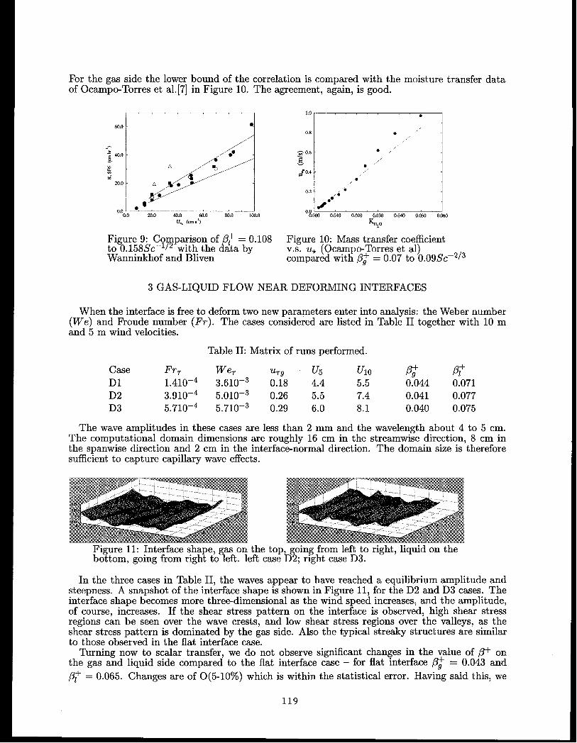
For the gas side the lower bound of the correlation is compared with the moisture transfer dataof Ocampo-Torres et al. [7] in Figure 10. The agreement, again, is good.

64,0●

--~ 40.0&

AE:

20.0 A

●O

0.00.0 20.0 40.0 .50.0 80.0 lCO.O

U., (cms“’)

Figure 9: Co parison of ~ = 0.108? Cfto 0.158Sc-l 2 with the ata by

Wanninkhof and Bliven

●

●

✘

:LO.cca0.0100.020 0,030 OC-40 0.0s0 c

%20

Figure 10: Mass transfer coefficientV.S. U* (Ocampo-Torres et al)compared with @ = 0.07 to 0.09SC–213

3 GAS-LIQUID FLOW NEAR DEFORMING INTERFACES

When the interface is free to deform two new parameters enter into analysis: the Weber number(We) and Froude number (1%). The cases considered are listed in Table II together with 10 mand 5 m wind velocities.

Table 11: Matrix of runs performed.

Case Fr7 Wer ‘T(J U5 Ulo P; @D1 1.410-4 3.610-3 0.18 4.4 5.5 0.044 0.071D2 3.910-4 5.010-3 0.26 5.5 7.4 0.041 0.077D3 5.710-4 5.710-3 0.29 6.0 8.1 0.040 0.075

The wave amplitudes in these cases are less than 2 mm and the wavelength about 4 to 5 cm.The computational domain dimensions are roughly 16 cm in the streamwise direction, 8 cm inthe spanwise direction and 2 cm in the interface-normal direction. The domain size is thereforesufficient to capture capillary wave effects.

Figure 11: Interface shape, gas on the top going from left to right, liquid on thebottom, going from right to left. left case ‘D2; right case D3.

In the three cases in Table II, the waves appear to have reached a equilibrium amplitude andsteepness. A snapshot of the interface shape is shown in Figure 11, for the D2 and D3 cases. Theinterface shape becomes more three-dimensional as the wind speed increases, and the amplitude,of course, increases. If the shear stress pattern on the interface is observed, high shear stressregions can be seen over the wave crests, and low shear stress regions over the valleys, as theshear stress pattern is dominated by the gas side. Also the typical streaky structures are similarto those observed in the flat interface case.

Turning now to scalar transfer, we do not observe significant changes in the value of Q+ onthe gas and liquid side compared to the flat interface case – for flat interface @ = 0.043 and

@ = 0.065. Changes are of 0(5-10%) which is within the statistical error. Having said this, we

119

do observe a slight trend. The value of /3+ on the liquid side is seen first to increase and then todecrease with wave amplitude. On the gas side we observe no significant change. The values areshown in Table II.

The modest increase of /3+ for small wave amplitude on the liquid side has also been observedby Komori et al.[8] in wind-wave tank experiments. Komori at al.[8] observed first a slight increaseof ~+ with wave amplitude and then a drop.

5 CONCI,USION

Maas transfer across gas-liquid interfaces has been studied. For flow over a flat interface theeffect of the Schmidt number has been investigated.. It has been found that large vertical (interface-normal) velocity fluctuations dominate the gas side flux whereas sweeps control the liquid sideflux. Both these scale with the friction velocity and support parametrization presented in thismanuscript.

When waves are allowed to form freely on a mobile interface, the value of ~+ is not signifi-cantly affected, indicating that the proposed parametrizations are still valid. It appears that suchparametrizations also carry over to more complex multiphase flows e.g. bubble columns whereCockx et al.1,9]has shown that the proposed correlation holds for the liquid side mass transfer.This is probably because the length scales associated with the sweeps are much smaller than thebubble size and the mean interface structures are similar to those in separated flows.

ACKNOWLEDGEMENT

The work was supported by the U.S. Department of Energy

References

GRANT DE-FG03-85ER-13314.

[1]

[2]

[3]

[4]

[5]

[6]

[7]

[8]

[9]

S.J. Kline. W.C. Revnolds. F.A. Schraub. and P.W. Runstadler. The structure of turbulentboundary ~ayers. J. >luids ‘iklech., 70:741, ‘1978.

M. Rashidi and S. Banerjee. The effect of boundary conditions and shear rates on streaksformation and breakdown in turbulent channel flow. Phys. Fluid,A2:1827, 1990.

P. Lombardi, V. De Angelis, and S. Banerjee. Direct numerical simulation of near-interfaceturbulence in coupled gas-liquid flow. Physics of Fluids, 8(6):1643-65, 1996.

S. Banerjee. A note on turbulent mass transfer at Klgh schmidt numbers. Chemical EngineeringScience, 26(6):989-90, 1971.

S. Banerjee. Turbulence structure and transport mechanisms at interfaces. Proceedings of theNinth International Heat Ikansfer Conference, Jerusalem, Israel, pages 395-417, 1990.

R.H. Wanninkhof and L.F. Bliven. Relationship between gas exchange, wind speed, and radarbackscatter in a large wind wave tank. J. of Geophys. Res., 96( C2):2785-2796, 1991.

F.J. Ocampo-Torres, F.J. Donelan, J.M. Wocdlen, and J.R. Koh. Laboratory measurements ofmass transfer of carbon dioxide and water vapor for smooth and rough flow conditions. TellusSeries B, 46:16, 1994.

S. Komcjri, R. Nagaosa, and Y. Murakami. ‘Turbulence structure and mass transfer across asheared air-water interface in wind-driven turbulence. Journal of Fluid Mechanics, 249:161–83,1993.

A. Cockx, M. Roustan, A. Line, and G. Hebrard. Modelling of mass transfer coefficient kl inbubble columns. Trans IChemE, 73-A:627, 1977.

120

INTERMITTENCY IN MODELS OF TURBULENCE

Robert H. Kraichnan

369 Montezuma 108, Santa Fe, New Mexico 87501

ABSTRACT

The intermittent statistics of the small scales of motion in fully de-veloped Navier-Stokes turbulence remain an outstanding challenge to re-searchers. Theoretical and computer studies of two simpler systems thatshare features with Navier-Stokes turbulence, and exhibit intermittence ofsmall scales, are described here. One is Burgers’ one-dimensional modelof turbulence. The statistics of velocity gradients and velocity differencesover small distances are found to exhibit a surprisingly complex structure.The second system is an ensemble of ideal vortices. Analysis of this systemimplies that the asymptotic scaling exponents for dissipation and squaredvorticity in Navier-Stokes turbulence must be equal.

INTRODUCTION

Approximate treatments of the statistics of Navier-Stokes turbulence that proceedsystematically from the equations of motion have given good qualitative, and even quan-titative, predictions of gross statistical properties like cascacle of energy. Higher statistics,particularly those associated with the observed intermittence of small spatial scales areanother story. Fractal models of small scales abound, but their connection with theequations of motion is almost nonexistent in most cases. Thus the small scales are anoutstanding challenge to theorists. The statistics of small scales are of practical impor-tance, for example in turbulent chemical reactions of non-premixed components.

Burgers’ equation describes a one-dimensional infinitely-compressible fluid. It leadsto dynamics quite distinct from that of the incompressible Navier-Stokes ecluation, butboth dynamics exhibit cascade of liinetic energy to small scales (large wavenumbers) and

121

the development of int ermittency at small scales. In the case of Burgers equation thesmall-scale interrnittency is associated with shock fronts, while in the lNavier-Stokes caseit is associated with intense vortex structures. Both equations have quadratic nonlinearity.Because of these similarities, Burgers equation has been a testing ground for analyticalapproaches aimed at the Navier-St ekes equation.

In the past few years a number of papers have attacked the problem of small-scaleintermit tency in Burgers equation, some invoking current methods of quantum field theory[1-9]. The work to be described here was carried out in collaboration with T. Gotoh [10].It combines some elementary analysis of ensembles of shocks with exact equations ofmotion for the probability density function (pdf ) of velocity gradient. The predictionswere tested by computer simulations. The pdf of gradient is found to have a surprisinglycomplex struct urea

High-Reynolds number Navier-Stokes turbulence exhibits intense worm-like vorticesthat live in a background of less-structured excitation. These vortices are thought todominate the higher-order moments of vorticity and the scaling exponents that describethe variation, as powers of r, of moments of the average over regions of size r of vorticit yand energy-dissipation. The dissipation associated with an intense cylindrical vortex liesout side the vortex core, and therefore is more spatially diffuse than the scluared vorticit y.This fact, together with analysis of high- Re:ynolds-number simulations and experimentshas led to the hypothesis that the growth of interrnittency of dissipation with decreaseof r is asymptotically slower than that of squared vorticity at infinite Reynolds number.That is, the high-order scaling exponents of dissipation are larger than those of squaredvort icit y.

In work to be summarized here, it is fou:nd that this conjectured asymptotic behaviorcannot be mediated by cylindrical vortices. The interrnittency of dissipation is numericallyless than that of squared vorticit y at large Reynolds number, but the associated ratiosare finite and do not increase indefinitely with Reynolds number. This work was done in

collaboration wit h G. He, S. Chen} R. Zhang, and Y. Zhou

BURGERS TURBULENCE FORCED AT LARGE SCALES

Burgers equation with forcing is

where u (x, t) is a one-dimensional velocity field and j(x, t) is a forcing term. The left sideof (1) is the Lagrangian time derivative of u, measured along a fluid-element trajectory.Differentiation of (1) yields

(2)

where ~ = uZ. The (2 term in (2) represents advective gradient intensification ordiminution along Lagrangian trajectories. Intensification occurs where ~ < 0, leadingto the formation of shock fronts. An isolated shock front at large R has the ideal form

f(x) a –(u~/v)sech2(u, z/2v), where 2u. is the jump in velocity across the shock.

We shall assume that the forcing changes infinitely rapidly in time, and is statisti-cally homogeneous and stationary, with compact spectral support concentrated about awavenumber kf. The intensity of forcing of the velocity gradient is measured by

where U(Z, t = O) = O and ( ) denotes ensemble average. A characteristic forcing strainrate and Reynolds number induced by the forcing may be defined by (f = B 113 and

R = ~f/(vk~). The steady-state values of rms velocity UT.ZS= (u )2 1/2

and typical shockjump induced by the forcing are both O((f /kf). The typical shock width is v/ur~~ andthe typical velocity gradient f = u, at the center of a shock is Rcf.

An exact equation of motion for the probability distribution function Q(t) of (follows from (3):

(4)

Here ~(~) ~ (~zz If) denotes the ensemble mean of (ZZ conditional on fixed ~. Thisrelation can be derived by following probabilities along Lagrangian trajectories [1,10].

The (2 term in (2) plays two opposed roles. If ~ <0, it intensifies the graclient but, atthe same time, squeezes the fluid and thereby decreases the measure along z associatedwith an interval d~. If f > 0, the gradient is decreased but measure is increased by

stretching of the fluid. The intensification or diminution of gradient is expressed in (4)by the d(f2 Q)/~f term and the rate of change of measure is expressed by the ~Q term.The 1? term in (4) expresses in standard fashion the outward diffusion of probability due

to infinitely-rapidly-changing forcing.

The v term in (4) expresses the relaxation of curvature of U(Z ). It smooths shocks.Regions where ~ >0 are flattened by advection. Thus it is reasonable to assume that thev term in (4) is negligible if ~ >> &f and R >> 1. The solution of (4) then has the form

where C+ is a dimensionless constant and the ineql~ality defines the range in which wehope the neglect of viscous effects is justified. The exponential factor in (5) was firstfound by Polyakov [4], but with a different prefa.ctor. Computer simulations support (5),but a decisive test is difficult because Q falls off so rapidly as ~ increases [10].

123

The behavior of Q for R >1, ~ <0 is more complicated. There is a central peakof width 0( ~f ), followed by a tail for –~ >> ~f. Qualitative analysis of (4) together withanalysis of the statistics of an ensemble of idealized sech2 shocks leads to the followingstructure fcm the tail. First there is an intermediate e region (f << –f << Rl 12( ~ whereQ(c) cx l~\--3. This represents the transient steepening of regions of negative gradient.Next there is a region Rz12~f << –~ << Rff where Q(c) cx 1/Rl~l. This region is supportedby the shoulders of mature, long-lived strong shocks. Finally there is a region –~ > R&’fwhere Q(~) falls off rapidly (faster than algebraically). This represents the cent ral regionsof st rong shock fronts. The structure described here is supported by computer simulationsin the range 1000 s R s 18000. See Fig. 1.

n

uw

Q

10-2t

-. \ .

\\‘. . . .

104t \\

‘\-* ‘\

-**,.

t -%.

t

\ \ \ \

,..6, ‘-~yi0 \

10-0

10-10-I, i #,

ml 10° 101 102 103 104 105Iw%f

Fig. 1. Logarithmic plot of (fQ(() vs l~llff for f <0 for three steady-state simulationswith Reyncdds numbers R = 15 (light dashed line), R = 1000 (heavy dashed line), andR = 18000 (solid line).

STATISTICS OF ENSEMBLES OF CYLINDRICAL VORTICES

It is known that that turbulent enstrophy density (squared vorticity magnitude) ismore intermittent than the density of dissipation of kinetic-energy. One measure of inter-mit tency of a quantity is the scaling exponents that measure how the ratios of momentsof local space averages of the quantity change as the averaging volume decreases. Recentmeasurements of these exponents computer simulations and experiments suggest that the

exponents of enst rophy and dissipation are different [11,12], with the implication that, atinfinite Reynolds number, enstrophy is infinitely more intermittent than dissipation.

In recent work, we raise the question of whether any kind of flow structure existsthat can support enstrophy that is infinitely more intermittent than dissipation [13]. Ifsuch structures do not exist, then the scaling exponents cannot be different as Reynoldsnumber tends to infinity. Our work was confined to cylindrical vortices but we believethe results are generally valid.

In a cylindrical vortex, the only velocity component is the azimuthal componentVe(r), where r is distance from the axis. The entrophy density and dissipation density(normalized by viscosity v) are

f--l(r) = ($+32‘(’”)=(*-:)2 (6)

The enstrophy and normalized dissipation per unit length of vortex are 2~ ~O@fl(r)r dr

and 27r~Ome(r)r dr, respectively. The moments

!2. = 2X/

‘[~(r)]nr dr, en = 2?r1“

[C(r)]nr dr (7)o 0

describe the distribution of enstrophy and dissipation densities in the single vortex struc-ture. By (6), fll = Cl if VO(0) = Ve(co) = O. The sizes of the ratios Rn = $2n/en aremeasures of how much greater enstrophy intermittence is than dissipation intermittence.

The simplest cylindrical vortex is the Rankin vortex of radius r. for which Ve cx r(r < ro) and VO M l/r (r > To). Here the vorticity is confined to a rigidly rotatingcore and all the dissipation lies outside the core. The ratios R,, calculated from (3) areRn = 2n – 1, corresponding to enstrophy that is modestly more spatially intermittentthan dissipation.

We have performed a calculus of variations analysis to find the velocity profile thatmaximizes Rn. The cylindrical vorticity distribution that maximizes R2 can be found bysolving the associated variational problem, wit h ~Omw(r)r dr and Q1 held constant. Theresult confirms what can be guessed by inspection of (fi): The maximizing dist ribut ion isthe limit rl /r. j co of

vo(r) cx r (r < r0)7 v~(r) cx ra (70 < r < rl), v~(r) m I/r (r> r,), (8)

125

with a = 1/2. In this case, Rn = (n – l)9n for n > 1. In particular, Rz = 81. Similarprofiles, with different values of a maximize R. for larger n.

The finiteness of these maximal intermittence ratios implies that there is no cylindri-cal vortex structure that supports asymptotically different scaling exponents for enstrophyand dissipation.

Neither the Rankin vortex nor the vortices with powerlaw cores just described satisfythe Navier-Stokes equation with finite viscosity. An idealized vortex that does satisfy the

equation is the Burgers vortex, which is an equilibrium solution in a uniform strainingfield. For it,

r 1– exp(–r2/r~)v~(r) = ~— 9 (9)

T

where I’ is the total circulation and rb measures the core diameter. From (6), O(r) w

exp(—2r2/r~ ), and the vorticity and dissipation overlap. Eq. (6) yields R2 m 10.65,R3 x 104.0’7, RA s 1040.02. To a rough approximation, R. w 10”– 1.

This investigation has demonstrated that any cylindriczd vortex gives finite momentratios Rn of enstropy to dissipation moments. It follows that no ensemble of cylindricalvortices can support different asymptotic scaling exponents for enst rophy and dissipationaveraged over a domain of size r. However, large finite values of the Rn are possible.In particulm they are achieved by the Burgers vortex, which is a solution of the Navier-Stokes equation. We have found that, as a consequence, ensembles of Burgers vorticescan emulate different scaling exponents for enst rophy and dissipation over finite rangesof r [13], in agreement with experimental measurements over finite ranges [12].

CONCLUDING REMARKS

The complexity of statistical structure exhibited by the probability distributions ofvelocity gITLdl1311tand velocity differences in 13urgers turbulence perhaps is surprising. The

question arises of whether this is an indicator that comparable complexity would be foundin the statistics of Navier-Stokes turbulence. Some insight may be provided by looking indetail at the statistics of ensembles of ideal vortices, in correspondence to the analysis ofensembles of ideal shocks for Burgers equation. ‘The work on moment ratios associatedwith ideal IBurgers vortices reported here is an elementary step in that direction.

.ACKNOWLEDGEMENT

This work was supported by Grant DE-FG03-90ER14118 to Robert H. Kraichnan,Inc. from the U. S. Department of Energy, Office of Basic Energy Sciences, EngineeringResearch Program.

REFERENCES

[1] T. Gotoh and R. H. Kraichnan, “Statistics of decaying Burgers Turbulence,” Phys.Fluids A 5, 445 (1993); T. Gotoh, “Inertial range statistics of Burgers turbulence,” Phys.Fluids 6, 3985 (1994).

[2] A. Chekhlov and V. Yakhot, “Kolmogorov turbulence in a random-force-driven Burgersequation,” Phys. Rev. E, 51, 2739 (1995); A. Chekhlov and V. Yakhot, “Kolrnogorovturbulence in a random-force-driven Burgers equation: anomalous scaling and probabilitydensity functions,” Phys. Rev. E 52, 5681 (1995).

[3] M. Avellaneda, R. Ryan, and Weinan E, “PDFs for velocity and velocity gradients inBurgers turbulence,” Phys. Fluids 7, 3067 (1995).

[4] A. M. Polyakov, “Turbulence without pressure,” Phys. Rev. E 52, 6183 (1995).

[5] J.-P. Bouchaud, M. M6zard, and G. Parisi, “Scaling and interrnittency in Burgersturbulence,” Phys. Rev. E 52, 3656 (1995); J.-P. Bouchaud and M. M6zard, “Velocityfluctuations in forced Burgers turbulence,” Phys. Rev. E 54, 5116 (1996).

[6] G. Falkovich, 1. Kolokolov, V. Lebedev, and A. Migdal, “Insta.ntons and intermittence,”Phys. Rev. E 54,4896 (1996).

[7] E. Balkovsky, G. Falkovich, L Kolokolov, and V. Lebedev, “Intermittence of Burgersturbulence,” Phys. Rev. Lett. 78, 1452 (1997).

[8] V. Gurarie and A. Migdal, “Instantons in the Burgers equation,” Phys. Rev. E 54,4908 (1996).

[9] Weinan E, K. Khanin, A, Mazel, and Y. Sinai, “Probability distribution functions forthe random forced Burgers equation,” Phys. Rev. Lett. 78, 1904 (1997).

[10] T. Gotoh and R. H. Kraichnan, “Burgers turbulence with large-scale forcing,” sub-mitted to Phys. Fluids (preprint: http: //xxx.lanl.gov/a.rchi\~e/cllao-d~~ll/98O3O37).

[11] S. Chen, K. R. Sreenivasan, M. Nelkin and N. Cao, “A refined similarity hypothesisfor tranverse structure functions,” Phys. Rev. Lett. 79, 1253 (1997), S. Chen, K. R.Sreenivasan and M. Nelkin, Phys. Rev. Lett. 79, 2253 (1997).

[12] K. R. Sreenivasan and R. A. Antonia, “The phenomenology of small-scale turbu-lence,” Annu. Rev. Fluid Mech., 29, 435 (1997).

[13] G. He, S. Chen, R, H. Kraichnan, R. Zhang, and Y. Zhou, “Statistics of dissipationand enstrophy induced by a set of Burgers vortices,?’ submitted to Phys. Rev. Let t.(preprint: http: //xxx.lanl.gov/archive/chao-dyn/98O3O29).

DYNAMICAL - STATISTICAL MOI)ELING OF TURBULENCE

E. A. Novikov

Institute for Nonlinear ScienceUniversity of California, San Diego

La Jolla, CA 92093-0402

ABSTRACT

A general approach to a dynamical-statistical modeling ofturbulence is described. The emphasis is on developmentsin conditional averaging, use of t~heinfinitely divisible

distributions, modeling of free-surface turbulence andturbulent boundary layers.

The major goal of turbulence modeling is to slave the enormous number ofdegrees of freedom in turbulent flows to a selected set of variables, manageable

by computer simulations. To do this properly we need to learn a lot about thestatistical structure of turbulent flows, which, of course, has independent interest.Different interconnected approaches to turbulence are employed in this work. Forexample, in the conditional averaging we get as far as we can by manipulatingdirectly with the Navier-Stokes equations (NSE). At the same time, we use general

statistical schemes, like Markov processes and infinitely divisible distributions,making them consistent with NSE and with experimental data. We also working

on some engineering tools, particularly, fc)r turbulent flows with complex geometry.A general strategy, developed in this wo:rk, is summarizes in the Diagram.

The upper horizontal row of four blocks in this Diagram represents various as-pects of statistical structure of turbulence and corresponding ingredients of mod-eling. The first block in this row refers to the Lagrangian and Eulerian descriptionof turbulence in terms of the Markov processes with dependent increments [1-3].

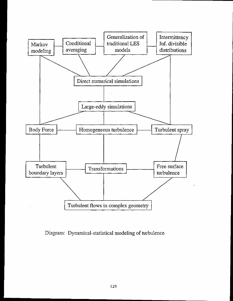
Intermittence

Markov Conditional Inf. divisible

modeling averaging distributions

I I

Generalization of

traditional LES

models/

Direct numerical simulations

Large-eddy simulations

Body Force Homogeneous turbulence — Turbulent spray

TurbulentTransformations

Free surface

boundary layers turbulence

I ITurbulent flows in complex geometry

129

Diagram: Dynamical-statistical modeling of turbulence

This Markov modeling is made statistically consistent with NSE and with ex-perimental data by using the exact relations between the Lagrangian and Eulerianstatistics [4].

Markov approach is connected with a body-force technique applicable to tur-bulent flows in complex geometry (see corresponding blocks in the Diagram).Body fmce relaxes fluid inside a body and. we use the Cartesian grid in numericalsimulations instead of the labor-consuming procedures of a mapping of the flowin complex geometry. Such technique is used for a fluid dynamics of the heart [5].We applied it to a free-surface turbulent jlow with a surface piercing body [6].

The second block in the upper row OFthe Diagram refers to conditional av-eraging of local characteristics (lc) of turbulent flows, which have an internalmechanism of amplification [7]. For three-dimensional (3D) turbulence lC is thevortici~y field and amplification is due to the vortex stret thing [8,9]. For 2D tur-bulence k is vorticity gradient (vg) and amplification is due to compression offluid particle in the direction of vg [10,11]. In both cases the deformation ratetensor, responsible for amplification, is expressed in terms of lC and we use theconcept of self-amplification. Conditional averaging of NSE written in terms oflc, with fixed lC in a point, transforms the major nonlinear amplification terminto a linear term [10,11]. This allows, particularly, an analytical study of theconditionally-averaged 3D vorticity field:

(1)

Here r is distance from the point with fixed vorticity U, ~1 and j2 are theone-point and two-point probability density functions (pd~) for the vorticity field.

We note that the conditionally-averagecl NSE with fixed vorticity in n pointscorresponds to a hierarchy of equations for the n-point pdj [9,11]. For the Fourier-transform of(1) we have general expression [11]:

where Ui = Wiw‘~,n~ = k~k-~ are unit vectors of vorticity and of the wave-number correspondingly, p = aini is their scalar product, eij~ is the unite anti-symmetric tensor. In expression (2) we used the local isotropy of turbulence andsolenoidality of the vorticity field. scalar g represents the viscous smoothing ofvorticity and it is symmetric function of p. Scalar h represents vortex stretchingand twisting and it is anti symmetric function of p. For turbulent flows with highReynollds number Re = VLV-l (V - characteristic velocity, L - external scale, v

- kinematic viscosity), it was analytically predicted [10,11] that vortex stretching

and twisting is statistically balanced with viscous smoothing on any level of fixed– 1/2. This predictionvorticity w and other terms in the vorticity balance are N Re

was confirmed by direct numerical simulations (DNS) [12,13], which also revealedthat the conditionally-averaged rates of vortex stretching and dissipation increaseexponentially with w. This exponential growth of two opposing physical effectscan provide a statistical environment for local instabilities and strong fluctuations- formation of strong localized vortices (“vortex strings”), followed by a quickbreakdown and twisting of such vortices when they become unstable. Such a pic-ture was observed experimentally [14], The whole conditionally-averaged vorticity(CAV) field (1) with twisting and hyperboloidal components (2) is obtained fromDNS [13]. The characteristic attenuation scale for CAV components is found tobe of order ten times bigger than the Kolmogorov microscale .lV= V314< s >-1/4,where < e > is the mean rate of the energy dissipation. The obtainedis in a qualitative agreement with simple analytical model [11]:

CAV field

(3)

where E(k) = 27r < fiiwi > is the energy spectrum. However, certain details

are different and in future we need a more accurate analytical description of CAV,which can be used in a relaxation subgrid-scale scheme [3,13] for the large-eddysimulations (LES).

It seems natural to choose the grid scale from the hierarchy of increasing scales

for coherent structures in 3D turbulence [15,16]:

l~~m = LRe-3it10+6m) (m = 0,1, 2...) (4)

These scales are obtained from a correlation analysis of NSE (with large-scalerandom forcing) by using a special functional formalism [17,18]. Particularly,

at the scale 1~ s t~) = LRe–3110 the nonlinear effects of vortex stretching and

convection do not produce flux in the vorticity correlations. Recent experimentaldata [19] supports the idea [15,16] that scales (4) are relevant to coherent “vortexstrings”. Analogous hierarchies of scales were obtained also for 2D turbulence fromcorrelation analysis of vg [16] and for passive scalars in 3D and 2D turbulence [20].

Conditional averaging was applied to the free-surface turbulence [21] with useof the fully nonlinear dynamical boundary conditions on free surface. Velocitycirculations in free-surface flows were also studied [22].

131

This leads us to another direction in the conditional averaging, connectedwith the use of local Lagrangian inviscid invariants of motion. For 3D turbulence

we introduced the micro circulations (velocity circulations over infinitesimal fluidcontours) [23]. To deal with finite quantities, we let:

Here s; is an oriented infinitesimal element of fluid surface, the initial areaof surface element SO is assumed, for simplicity, to be the same for all points

and we consider simultaneously three elements a; (a = 1,2, 3), which are initiallyorthogonal: o~of’ = 6aP at t = O. From NSE, written in terms of vorticity:

dui = b’ui+.,:”

t L3vi

x–z— = ‘wk + vAw~ ,

f%k(6)

i

with use of the incompressibility y, we get:

(7)

These equations, in a sense, separate the effects of viscous smoothing andstretching of vorticity. Based on (7), by using the conditional averaging (with fixedvortici~y), a statistical evolution of rnicrocirculations and fluid surface elementsare studied (particularly, initial tendencies) with various initial orientations offluid contours relative to the vorticity field [23].

For 2D turbulence, we introduced the Lagrangian infinitesimal increments ofvorticit y [24]:

(8)

Here r? (a = 1,2) are linear infinitesimal fluid elements with initial length ro(the saline for all points) and initially orthogonal: p~p~ = ~ap. From NSE, writtenin terms of vg:

dsi ~vk—=dt

‘—”sk + v@,ax~

using the incompressibility, we get:

d& dp~ & ~—=

dtvp~Asi, — = —

dt axk ‘k

132!

(9)

(lo)

These equations separate the effects of linear diffusion and nonlinear sharpen-ing of vg. From (10), by using conditional averaging (with fixed vg), we studiedstatistical evolution of vorticity increments and fluid elements with various mutualorientations [24]. We also used the fact, established in our numerical experiments

[25]:

&J~ .%sk <0/0(s) = ——

bk S2(11)

Here overbar means conditional averaging with fixed vg, /3(s) is the condition-ally averaged deformation rate with fixed Si. The physical meaning of inequality

(11) is that the effect of nonlinear sharpening of vg in 2D turbulence statisticallypersists on all levels of s.

The third block in the upper row in the Diagram refers to traditional subgrid-scale (SGS) models (Smagorinsky [26], 13ardina [27]) and their broad generaliza-tions [28,29]. These models, generally, can serve some engineering goals. However,they may insufficiently reflect the physics of turbulence. Particularly, the widelyused Smagorinsky model, by design, reproduce the “5/3” energy spectrum

( E(k) N< e >213 Ic-’i’ ), but our numerical experiments show that thismodel gives incorrect third order moment (flux of energy) and incorrect highorder moments (intermittence).

This leads us to the last block in the upper row. The effects of intermittenceare described in terms of the breakdown coefficients (Me) for the energy dissipa-tion [30]. These bdc are shown to be an alternative to the multifractal formalism

[1]. An intermittence correction was obtained for a simple SGS model [1]. Thephenomena of scale similarity and intermittence were imbedded into the theory ofthe infinitely divisible distributions [31]. This allows USto use the well developed

mathematical apparatus [32]. The results are compared with experimental data

corresponding to Re N 107[33]. The bdc approach and the theory of infinitelydivisible distributions were recently applied to the phenomena of turbulent spray

[34] (see corresponding block in the Diagram) and can be readily applied to tur-bulent bubble flows. Turbulent spray and bubble flows are important in manyareas of engineering.

Related to this is our work on more general problems of the free-surface turbu-lence [29,35]. Here, along with high resolution I)NS, we use some transformationsfrom homogeneous to nonhomogeneous turbulence [36] and a level set approach

[6], which significantly simplifies numerical simulations, For free-surface turbu-lent flows with surface piercing bodies, as a starting point, we used the following

133

transformation:

(12)

Here vi is the velocity fluctuation in a nonhomogeneous turbulent flow with themean velocity profile u., ; velocity Wi , prc~duced by LES, is solenoidal (~ = O)

and statistically homogeneous in horizontal plane (with a nonlinear free-surfaceapproacl~ or a low Frude-number approximation); constant c we can put equalto zero for a turbulent wake; bi is a deformation of the flow and, in first approx-

imation, we used b; = Tui , where T is a characteristic time of the flow. Thevelocity field (12) is solenoidal and if we choose T constant, then deformation isalso sole:noidal and the last term in (12) is zero (with c = O). Transformation (12)is suggested by the Poisson-bracket form of the nonlinear terms in NSE. Compari-son of this transformation with experimental data [36] shows, that the correlationcoefficient, calculated in terms of turbulent energy ~ < v: > , is surprisingly high(~ ().s). Transformation (12), which is designed for a distant part of the wake,

can be generalized, for example, by using several successive transformations inorder to get closer to a body.

Another development is in the modeling of turbulent boundary layers (TBL).Such modeling is important by itself and also is very useful for a boundary con-dition in LES. A variational approach to TBL is developed [37]. Particularly, fora turbulent flow along a cylinder with radius a, we get the following equation forthe mean velocity profile u(r):

(13)

Here 6/tk stands for the variational (functional) derivative, ~ is the eigenvalueof this variational operator applied to the enst rophy of the mean flow. A unique

solution of this equation, which recovers the standard logarithmic profile (for theflat boundary) on distances z = r – a << a , has the form:

u = ~{ln[a+ ln(z+/a+ + I)] + b}K

(14)

Here u. is the friction velocity, K = (II.4 is the Karman constant, a+ = a/.z*,

z’* = V/U* is the thickness of the viscous sublayer, z+ = z/z* and b ~ 2 isthe empirical constant in the standard logarithmic profile, correspondkg to ahydrodpamically smooth boundary. The variational eigenvalue A = ~/u* is,

thus, determined by the momentum flux, which is equal to u ~. Experimental data

fits well [37] into the double-logarittilc profile (14).Various aspects of turbulence, represented by blocks in the Diagram, are fruit-

ful areas of research. By putting them together, we reveal the important connec-tions, leading to more general methods of turbulence modeling.

ACKNOWLEDGMENT

This work is supported by the U. S. Department of Energy.

REFERENCES

1. E. A. NOVIKOV, Phys. Fluids Al, 326 (1989); Phys. Fluids A2, 814

(1990); Phys.Rev. A46(10), R6147 (1992).

2. G. PEDRIZZETTI and E. A. NOVIKOV, J. Fluid Mech. 280, 69 (1994).3. E. A. NOVIKOV, “Conditionally-averaged dynamics of turbulence, new

scaling and stochastic modeling”, in “L&JyFlights and Related Topics in Physics”

(eds. M. Schlesinger, G. Zaslavsky and U. Frish), pp 35-50, Springer, 1995.4. E. A. NOVIKOV, Appl. Math. Mech. 33, 862 (1969); Phys. Fluids 29,

3907 (1986). .

5. C, S. PESKINj Bull. Amer. Phys. Sot. 42 (11),2207 (1997).6. D. G. DOMMERMUTH, E. A. SCHLAGETER, J. C. TALCOTT, D. C.

WYATT and E. A. NOVIKOV, Butl. Amer. Phys. Sot. 42 (11), 2196 (1997),also preprint.

7. E. A. NOVIKOV, Fluid Dyn. Res. 6, 79 (1990).8. G. I. TAYLOR, Proc. Roy. Sot. London A164, 15 (1938).9. E. A. NOVIKOV, Dokl. Akad. Nauk SSSR 12, 299, (1967) [Sov. Phys.

Dok/. 12, 1006 (1968)1.

10. E. A. NOVIKOV, “Solution of exact kinetic equations for intermittentturbulence”, Proc. of Monte-Verita Sympos. (1991), New Approaches and Con-cepts in Turbulence (edited by T. Dracos and A. Tsinober), Birkauser, Basel,pp.131-139, 1993; Phys. Lett. A162, 385 (1992); J. Phys. A25, L657 (1992);

“Exact results obtained by conditional averaging of Navier-Stokes equations”, inTurbulence in Spatially Extended Systems (eds. R. Benzi, C. Basdevant and S.Chiliberti), pp. 101-106, Nova Scince Publishers, 1993.

11. E. A. NOVIKOV, Fluid Dyn. Res. 12, 107 (1993).12. E. A. NOVIKOV and D. G. DOM?vlERMuTH, Modern Phys.Lett. B8

135

(23), 13!15 (1994).13. R. C. Y. MUI, D. G. DOMMERM~JTH and E. A. NOVIKOV, Phys. Rev.

E53 (3), 2355 (1996).14. S. DOUADY, Y. COUDER and M. E. BRACHET, Phys. Rev. Lett. 67,

983 (1991), and video produced by these authors.15. E. A. NOVIKOV, Phys. Rev. Lett. 71(17), 2718 (1993).

16. E. A. NOVIKOV, Phys. Rev. E49(2), R975 (1994).17. E. A. NOVIKOV, Zh. Eksp. Teor. Phys. 47, 1919 (1964) [Sov. Phys.

JETP 20, 1290 (1965)].18. W. D. McCOMB, The Physics l~fFluid turbulence, Claredon, Oxford,

1990, p. 554 (Appendix H).19. P. TABELING, private communication (1998).20. E. A. NOVIKOV, J. Phys. A, Math. Gen., 27 L797 (1994).

21. ‘E. A. NOVIKOV, Phys. Rev. E52, 5679 (1995).22. E. A. NOVIKOV, Int. J. Eng. Sci. 34, 359 (1995).23. E. A. NOWKOV, Phys. Rev. E5:2(3), 2574 (1995).24. E. A. NOVIKOV, Phys. Lett. A236, 65 (1997).25. A. E. NOVIKOV and E. A. NOVIKOV, in preparation.26. J. SMAGORINSKY, Mon. Weather Rev. 91, 99 (1963).

27. J. BARDINA, J. H. FERZIGER and W. C. REYNOLDS, AIAA 80-1357(1980).

28. T. S. LUND and E. A. NOVIKOV, Ann. Res., Stanford, 27 (1992).29. D. G. DOMMERMUTH and E. A. NOVIKOV, “Direct-numerical and

large-eddy simulations of turbulent free-surface flows”, Proc. Sixth Internat.Conf. on Numerical Ship Hydrodynamics, Iowa City, pp.239-270 (1993).

30. E. A. NOVIKOV, Appl. Math. Mech. 35, 231 (1971).31. E. A. NOVIKOV, Phys. Rev. E50(5), R3303 (1994).32. W. FELLER, An Introduction to Probability Theory and its Applications,

V.2, Wiley, 1991, reprint from 1966-edition.

33. G. PEDRIZZETTI, E. A. NOVIKOV and A. A. PRASKOVSKY, Phys.Rev. E53(1), 475 (1996).

34. E. A. NOVIKOV and D. G. DOMMERMUTH, Phys. Rev. E56(5), 5479(1997).

35. D. G. DOMMERMUTH, E. A. NOVIKOV and R. C. Y. MUI, “Theinteraction of surface waves with turbulence’), Proc. of ASMA Symp. on Free-Surface Turbulence, Lake Tahoe, 20 pages, 1994.

136

36.D. G. DOMMERMUTH, M. GHARIB, H. T. HUANG, G. I. INNIS, P.MAHEO, E. A. NOVIKOV, J. C. TALCOTT and D. C. WAYATT, “Turbulent

free-surface flows: a comparison between numerical simulations and experimen-

tal measurements”, Proc. 21-st Symp. on Naval Hydrodynamics, Trondheim,Norway, 17 pages, 1996.

37. E. A. NOVIKOV and D. G. DOMMERMUTH, “A variational approachto turbulent boundary layers”, in Fundamental Problematic Issues in Turbulence(eds. A. Gyr, P. Monkiewitz and A. Tsinober), Birkauser, Basel, 1998, to bepublished.

137