mixOmics: Omics Data Integration Project

Package ‘mixOmics’December 28, 2021

Type Package

Title Omics Data Integration Project

Version 6.18.1

Depends R (>= 3.5.0), MASS, lattice, ggplot2

Imports igraph, ellipse, corpcor, RColorBrewer, parallel, dplyr,tidyr, reshape2, methods, matrixStats, rARPACK, gridExtra,grDevices, graphics, stats, ggrepel, BiocParallel, utils

Suggests BiocStyle, knitr, rmarkdown, testthat, rgl

Maintainer Al J Abadi <[email protected]>

Description Multivariate methods are well suited to large omics data sets where the number of vari-ables (e.g. genes, proteins, metabolites) is much larger than the number of samples (pa-tients, cells, mice). They have the appealing properties of reducing the dimen-sion of the data by using instrumental variables (components), which are defined as combina-tions of all variables. Those components are then used to produce useful graphical out-puts that enable better understanding of the relationships and correlation structures be-tween the different data sets that are integrated. mixOmics offers a wide range of multivari-ate methods for the exploration and integration of biological datasets with a particular fo-cus on variable selection. The package proposes several sparse multivariate models we have de-veloped to identify the key variables that are highly correlated, and/or explain the biological out-come of interest. The data that can be analysed with mixOmics may come from high through-put sequencing technologies, such as omics data (transcriptomics, metabolomics, pro-teomics, metagenomics etc) but also beyond the realm of omics (e.g. spectral imag-ing). The methods implemented in mixOmics can also handle missing values without hav-ing to delete entire rows with missing data. A non exhaustive list of methods include vari-ants of generalised Canonical Correlation Analysis, sparse Partial Least Squares and sparse Dis-criminant Analysis. Recently we implemented integrative methods to combine multi-ple data sets: N-integration with variants of Generalised Canonical Correlation Analysis and P-integration with variants of multi-group Partial Least Squares.

License GPL (>= 2)

URL http://www.mixOmics.org

BugReports https://github.com/mixOmicsTeam/mixOmics/issues/

Repository Bioconductor

1

http://www.mixOmics.org

https://github.com/mixOmicsTeam/mixOmics/issues/

2 R topics documented:

VignetteBuilder knitr

Date 2021-07-15

NeedsCompilation no

biocViews ImmunoOncology, Microarray, Sequencing, Metabolomics,Metagenomics, Proteomics, GenePrediction, MultipleComparison,Classification, Regression

RoxygenNote 7.1.2

Encoding UTF-8

git_url https://git.bioconductor.org/packages/mixOmics

git_branch RELEASE_3_14

git_last_commit 5ef4960

git_last_commit_date 2021-11-17

Date/Publication 2021-12-28

Author Kim-Anh Le Cao [aut],Florian Rohart [aut],Ignacio Gonzalez [aut],Sebastien Dejean [aut],Al J Abadi [ctb, cre],Benoit Gautier [ctb],Francois Bartolo [ctb],Pierre Monget [ctb],Jeff Coquery [ctb],FangZou Yao [ctb],Benoit Liquet [ctb]

R topics documented:mixOmics-package . . . . . . . . . . . . . . . . . . . . . . . . . . . . . . . . . . . . . 4auroc . . . . . . . . . . . . . . . . . . . . . . . . . . . . . . . . . . . . . . . . . . . . 5background.predict . . . . . . . . . . . . . . . . . . . . . . . . . . . . . . . . . . . . . 10biplot . . . . . . . . . . . . . . . . . . . . . . . . . . . . . . . . . . . . . . . . . . . . 12block.pls . . . . . . . . . . . . . . . . . . . . . . . . . . . . . . . . . . . . . . . . . . . 16block.plsda . . . . . . . . . . . . . . . . . . . . . . . . . . . . . . . . . . . . . . . . . 19block.spls . . . . . . . . . . . . . . . . . . . . . . . . . . . . . . . . . . . . . . . . . . 22block.splsda . . . . . . . . . . . . . . . . . . . . . . . . . . . . . . . . . . . . . . . . . 26breast.TCGA . . . . . . . . . . . . . . . . . . . . . . . . . . . . . . . . . . . . . . . . 30breast.tumors . . . . . . . . . . . . . . . . . . . . . . . . . . . . . . . . . . . . . . . . 31cim . . . . . . . . . . . . . . . . . . . . . . . . . . . . . . . . . . . . . . . . . . . . . 32cimDiablo . . . . . . . . . . . . . . . . . . . . . . . . . . . . . . . . . . . . . . . . . . 40circosPlot . . . . . . . . . . . . . . . . . . . . . . . . . . . . . . . . . . . . . . . . . . 42colors . . . . . . . . . . . . . . . . . . . . . . . . . . . . . . . . . . . . . . . . . . . . 46diverse.16S . . . . . . . . . . . . . . . . . . . . . . . . . . . . . . . . . . . . . . . . . 48estim.regul . . . . . . . . . . . . . . . . . . . . . . . . . . . . . . . . . . . . . . . . . 49explained_variance . . . . . . . . . . . . . . . . . . . . . . . . . . . . . . . . . . . . . 50

R topics documented: 3

get.confusion_matrix . . . . . . . . . . . . . . . . . . . . . . . . . . . . . . . . . . . . 51image.tune.rcc . . . . . . . . . . . . . . . . . . . . . . . . . . . . . . . . . . . . . . . . 53imgCor . . . . . . . . . . . . . . . . . . . . . . . . . . . . . . . . . . . . . . . . . . . 54impute.nipals . . . . . . . . . . . . . . . . . . . . . . . . . . . . . . . . . . . . . . . . 56ipca . . . . . . . . . . . . . . . . . . . . . . . . . . . . . . . . . . . . . . . . . . . . . 57Koren.16S . . . . . . . . . . . . . . . . . . . . . . . . . . . . . . . . . . . . . . . . . . 59linnerud . . . . . . . . . . . . . . . . . . . . . . . . . . . . . . . . . . . . . . . . . . . 61liver.toxicity . . . . . . . . . . . . . . . . . . . . . . . . . . . . . . . . . . . . . . . . . 61logratio-transformations . . . . . . . . . . . . . . . . . . . . . . . . . . . . . . . . . . 63map . . . . . . . . . . . . . . . . . . . . . . . . . . . . . . . . . . . . . . . . . . . . . 64mat.rank . . . . . . . . . . . . . . . . . . . . . . . . . . . . . . . . . . . . . . . . . . . 65mint.block.pls . . . . . . . . . . . . . . . . . . . . . . . . . . . . . . . . . . . . . . . . 66mint.block.plsda . . . . . . . . . . . . . . . . . . . . . . . . . . . . . . . . . . . . . . . 69mint.block.spls . . . . . . . . . . . . . . . . . . . . . . . . . . . . . . . . . . . . . . . 72mint.block.splsda . . . . . . . . . . . . . . . . . . . . . . . . . . . . . . . . . . . . . . 75mint.pca . . . . . . . . . . . . . . . . . . . . . . . . . . . . . . . . . . . . . . . . . . . 79mint.pls . . . . . . . . . . . . . . . . . . . . . . . . . . . . . . . . . . . . . . . . . . . 80mint.plsda . . . . . . . . . . . . . . . . . . . . . . . . . . . . . . . . . . . . . . . . . . 83mint.spls . . . . . . . . . . . . . . . . . . . . . . . . . . . . . . . . . . . . . . . . . . . 86mint.splsda . . . . . . . . . . . . . . . . . . . . . . . . . . . . . . . . . . . . . . . . . 89mixOmics . . . . . . . . . . . . . . . . . . . . . . . . . . . . . . . . . . . . . . . . . . 92multidrug . . . . . . . . . . . . . . . . . . . . . . . . . . . . . . . . . . . . . . . . . . 96nearZeroVar . . . . . . . . . . . . . . . . . . . . . . . . . . . . . . . . . . . . . . . . . 98network . . . . . . . . . . . . . . . . . . . . . . . . . . . . . . . . . . . . . . . . . . . 99nipals . . . . . . . . . . . . . . . . . . . . . . . . . . . . . . . . . . . . . . . . . . . . 104nutrimouse . . . . . . . . . . . . . . . . . . . . . . . . . . . . . . . . . . . . . . . . . 105pca . . . . . . . . . . . . . . . . . . . . . . . . . . . . . . . . . . . . . . . . . . . . . . 106perf . . . . . . . . . . . . . . . . . . . . . . . . . . . . . . . . . . . . . . . . . . . . . 110plot.pca . . . . . . . . . . . . . . . . . . . . . . . . . . . . . . . . . . . . . . . . . . . 119plot.perf . . . . . . . . . . . . . . . . . . . . . . . . . . . . . . . . . . . . . . . . . . . 120plot.perf.pls . . . . . . . . . . . . . . . . . . . . . . . . . . . . . . . . . . . . . . . . . 122plot.rcc . . . . . . . . . . . . . . . . . . . . . . . . . . . . . . . . . . . . . . . . . . . 124plot.tune . . . . . . . . . . . . . . . . . . . . . . . . . . . . . . . . . . . . . . . . . . . 125plotArrow . . . . . . . . . . . . . . . . . . . . . . . . . . . . . . . . . . . . . . . . . . 129plotDiablo . . . . . . . . . . . . . . . . . . . . . . . . . . . . . . . . . . . . . . . . . . 133plotIndiv . . . . . . . . . . . . . . . . . . . . . . . . . . . . . . . . . . . . . . . . . . . 135plotLoadings . . . . . . . . . . . . . . . . . . . . . . . . . . . . . . . . . . . . . . . . 149plotMarkers . . . . . . . . . . . . . . . . . . . . . . . . . . . . . . . . . . . . . . . . . 161plotVar . . . . . . . . . . . . . . . . . . . . . . . . . . . . . . . . . . . . . . . . . . . . 162pls . . . . . . . . . . . . . . . . . . . . . . . . . . . . . . . . . . . . . . . . . . . . . . 167plsda . . . . . . . . . . . . . . . . . . . . . . . . . . . . . . . . . . . . . . . . . . . . . 171predict . . . . . . . . . . . . . . . . . . . . . . . . . . . . . . . . . . . . . . . . . . . . 174print . . . . . . . . . . . . . . . . . . . . . . . . . . . . . . . . . . . . . . . . . . . . . 179rcc . . . . . . . . . . . . . . . . . . . . . . . . . . . . . . . . . . . . . . . . . . . . . . 183selectVar . . . . . . . . . . . . . . . . . . . . . . . . . . . . . . . . . . . . . . . . . . . 186sipca . . . . . . . . . . . . . . . . . . . . . . . . . . . . . . . . . . . . . . . . . . . . . 188spca . . . . . . . . . . . . . . . . . . . . . . . . . . . . . . . . . . . . . . . . . . . . . 190spls . . . . . . . . . . . . . . . . . . . . . . . . . . . . . . . . . . . . . . . . . . . . . 193

4 mixOmics-package

splsda . . . . . . . . . . . . . . . . . . . . . . . . . . . . . . . . . . . . . . . . . . . . 198srbct . . . . . . . . . . . . . . . . . . . . . . . . . . . . . . . . . . . . . . . . . . . . . 202stemcells . . . . . . . . . . . . . . . . . . . . . . . . . . . . . . . . . . . . . . . . . . 203study_split . . . . . . . . . . . . . . . . . . . . . . . . . . . . . . . . . . . . . . . . . . 204summary . . . . . . . . . . . . . . . . . . . . . . . . . . . . . . . . . . . . . . . . . . 205tune . . . . . . . . . . . . . . . . . . . . . . . . . . . . . . . . . . . . . . . . . . . . . 207tune.block.splsda . . . . . . . . . . . . . . . . . . . . . . . . . . . . . . . . . . . . . . 211tune.mint.splsda . . . . . . . . . . . . . . . . . . . . . . . . . . . . . . . . . . . . . . . 216tune.pca . . . . . . . . . . . . . . . . . . . . . . . . . . . . . . . . . . . . . . . . . . . 219tune.rcc . . . . . . . . . . . . . . . . . . . . . . . . . . . . . . . . . . . . . . . . . . . 221tune.spca . . . . . . . . . . . . . . . . . . . . . . . . . . . . . . . . . . . . . . . . . . 222tune.spls . . . . . . . . . . . . . . . . . . . . . . . . . . . . . . . . . . . . . . . . . . . 224tune.splsda . . . . . . . . . . . . . . . . . . . . . . . . . . . . . . . . . . . . . . . . . 228tune.splslevel . . . . . . . . . . . . . . . . . . . . . . . . . . . . . . . . . . . . . . . . 232unmap . . . . . . . . . . . . . . . . . . . . . . . . . . . . . . . . . . . . . . . . . . . . 234vac18 . . . . . . . . . . . . . . . . . . . . . . . . . . . . . . . . . . . . . . . . . . . . 235vac18.simulated . . . . . . . . . . . . . . . . . . . . . . . . . . . . . . . . . . . . . . . 236vip . . . . . . . . . . . . . . . . . . . . . . . . . . . . . . . . . . . . . . . . . . . . . . 237withinVariation . . . . . . . . . . . . . . . . . . . . . . . . . . . . . . . . . . . . . . . 238wrapper.rgcca . . . . . . . . . . . . . . . . . . . . . . . . . . . . . . . . . . . . . . . . 239wrapper.sgcca . . . . . . . . . . . . . . . . . . . . . . . . . . . . . . . . . . . . . . . . 242yeast . . . . . . . . . . . . . . . . . . . . . . . . . . . . . . . . . . . . . . . . . . . . . 245

Index 246

mixOmics-package ’Omics Data Integration Project

Description

Multivariate methods are well suited to large omics data sets where the number of variables (e.g.genes, proteins, metabolites) is much larger than the number of samples (patients, cells, mice).They have the appealing properties of reducing the dimension of the data by using instrumentalvariables (components), which are defined as combinations of all variables. Those components arethen used to produce useful graphical outputs that enable better understanding of the relationshipsand correlation structures between the different data sets that are integrated.

Details

mixOmics offers a wide range of multivariate methods for the exploration and integration of biolog-ical datasets with a particular focus on variable selection. The package proposes several sparse mul-tivariate models we have developed to identify the key variables that are highly correlated, and/orexplain the biological outcome of interest. The data that can be analysed with mixOmics may comefrom high throughput sequencing technologies, such as omics data (transcriptomics, metabolomics,proteomics, metagenomics etc) but also beyond the realm of omics (e.g. spectral imaging).

The methods implemented in mixOmics can also handle missing values without having to deleteentire rows with missing data. A non exhaustive list of methods include variants of generalised

auroc 5

Canonical Correlation Analysis, sparse Partial Least Squares and sparse Discriminant Analysis.Recently we implemented integrative methods to combine multiple data sets: N-integration withvariants of Generalised Canonical Correlation Analysis and P-integration with variants of multi-group Partial Least Squares.

auroc Area Under the Curve (AUC) and Receiver Operating Characteristic(ROC) curves for supervised classification

Description

Calculates the AUC and plots ROC for supervised models from s/plsda, mint.s/plsda and block.plsda,block.splsda or wrapper.sgccda functions.

Usage

auroc(object, ...)

## S3 method for class 'mixo_plsda'auroc(object,newdata = object$input.X,outcome.test = as.factor(object$Y),multilevel = NULL,plot = TRUE,roc.comp = NULL,title = NULL,print = TRUE,...

)

## S3 method for class 'mixo_splsda'auroc(object,newdata = object$input.X,outcome.test = as.factor(object$Y),multilevel = NULL,plot = TRUE,roc.comp = NULL,title = NULL,print = TRUE,...

)

## S3 method for class 'mint.plsda'auroc(object,

6 auroc

newdata = object$X,outcome.test = as.factor(object$Y),study.test = object$study,multilevel = NULL,plot = TRUE,roc.comp = NULL,roc.study = "global",title = NULL,print = TRUE,...

)

## S3 method for class 'mint.splsda'auroc(object,newdata = object$X,outcome.test = as.factor(object$Y),study.test = object$study,multilevel = NULL,plot = TRUE,roc.comp = NULL,roc.study = "global",title = NULL,print = TRUE,...

)

## S3 method for class 'sgccda'auroc(object,newdata = object$X,outcome.test = as.factor(object$Y),multilevel = NULL,plot = TRUE,roc.block = 1L,roc.comp = NULL,title = NULL,print = TRUE,...

)

## S3 method for class 'mint.block.plsda'auroc(object,newdata = object$X,study.test = object$study,outcome.test = as.factor(object$Y),multilevel = NULL,

auroc 7

plot = TRUE,roc.block = 1,roc.comp = NULL,title = NULL,print = TRUE,...

)

## S3 method for class 'mint.block.splsda'auroc(object,newdata = object$X,study.test = object$study,outcome.test = as.factor(object$Y),multilevel = NULL,plot = TRUE,roc.block = 1,roc.comp = NULL,title = NULL,print = TRUE,...

)

Arguments

object Object of class inherited from one of the following supervised analysis func-tion: "plsda", "splsda", "mint.plsda", "mint.splsda", "block.splsda" or "wrap-per.sgccda"

... external optional arguments for plotting - line.col for custom colors and legend.titlefor custom legend title

newdata numeric matrix of predictors, by default set to the training data set (see details).

outcome.test Either a factor or a class vector for the discrete outcome, by default set to theoutcome vector from the training set (see details).

multilevel Sample information when a newdata matrix is input and when multilevel de-composition for repeated measurements is required. A numeric matrix or dataframe indicating the repeated measures on each individual, i.e. the individualsID. See examples in splsda.

plot Whether the ROC curves should be plotted, by default set to TRUE (see details).

roc.comp Specify the component (integer) up to which the ROC will be calculated andplotted from the multivariate model, default to 1.

title Character, specifies the title of the plot.

print Logical, specifies whether the output should be printed.

study.test For MINT objects, grouping factor indicating which samples of newdata arefrom the same study. Overlap with object$study are allowed.

roc.study Specify the study for which the ROC will be plotted for a mint.plsda or mint.splsdaobject, default to "global".

8 auroc

roc.block Specify the block number (integer) or the name of the block (set of characters)for which the ROC will be plotted for a block.plsda or block.splsda object, de-fault to 1.

Details

For more than two classes in the categorical outcome Y, the AUC is calculated as one class vs. theother and the ROC curves one class vs. the others are output.

The ROC and AUC are calculated based on the predicted scores obtained from the predict func-tion applied to the multivariate methods (predict(object)$predict). Our multivariate supervisedmethods already use a prediction threshold based on distances (see predict) that optimally deter-mine class membership of the samples tested. As such AUC and ROC are not needed to estimatethe performance of the model (see perf, tune that report classification error rates). We providethose outputs as complementary performance measures.

The pvalue is from a Wilcoxon test between the predicted scores between one class vs the others.

External independent data set (newdata) and outcome (outcome.test) can be input to calculateAUROC. The external data set must have the same variables as the training data set (object$X).

If newdata is not provided, AUROC is calculated from the training data set, and may result inoverfitting (too optimistic results).

Note that for mint.plsda and mint.splsda objects, if roc.study is different from "global", thennewdata), outcome.test and sstudy.test are not used.

Value

Depending on the type of object used, a list that contains: The AUC and Wilcoxon test pvalue foreach ’one vs other’ classes comparison performed, either per component (splsda, plsda, mint.plsda,mint.splsda), or per block and per component (wrapper.sgccda, block.plsda, blocksplsda).

Author(s)

Benoit Gautier, Francois Bartolo, Florian Rohart, Al J Abadi

See Also

tune, perf, and http://www.mixOmics.org for more details.

Examples

## example with PLSDA, 2 classes# ----------------data(breast.tumors)X <- breast.tumors$gene.expY <- breast.tumors$sample$treatment

plsda.breast <- plsda(X, Y, ncomp = 2)auc.plsda.breast = auroc(plsda.breast, roc.comp = 1)auc.plsda.breast = auroc(plsda.breast, roc.comp = 2)

## Not run:

auroc 9

## example with sPLSDA# -----------------splsda.breast <- splsda(X, Y, ncomp = 2, keepX = c(25, 25))auroc(plsda.breast, plot = FALSE)

## example with sPLSDA with 4 classes# -----------------data(liver.toxicity)X <- as.matrix(liver.toxicity$gene)# Y will be transformed as a factor in the function,# but we set it as a factor to set up the colors.Y <- as.factor(liver.toxicity$treatment[, 4])

splsda.liver <- splsda(X, Y, ncomp = 2, keepX = c(20, 20))auc.splsda.liver = auroc(splsda.liver, roc.comp = 2)

## example with mint.plsda# -----------------data(stemcells)

res = mint.plsda(X = stemcells$gene, Y = stemcells$celltype, ncomp = 3,study = stemcells$study)auc.mint.pslda = auroc(res, plot = FALSE)

## example with mint.splsda# -----------------res = mint.splsda(X = stemcells$gene, Y = stemcells$celltype, ncomp = 3, keepX = c(10, 5, 15),study = stemcells$study)auc.mint.spslda = auroc(res, plot = TRUE, roc.comp = 3)

## example with block.plsda# ------------------data(nutrimouse)data = list(gene = nutrimouse$gene, lipid = nutrimouse$lipid)# with this design, all blocks are connecteddesign = matrix(c(0,1,1,0), ncol = 2, nrow = 2,byrow = TRUE, dimnames = list(names(data), names(data)))

block.plsda.nutri = block.plsda(X = data, Y = nutrimouse$diet)auc.block.plsda.nutri = auroc(block.plsda.nutri, roc.block = 'lipid')

## example with block.splsda# ---------------list.keepX = list(gene = rep(10, 2), lipid = rep(5,2))block.splsda.nutri = block.splsda(X = data, Y = nutrimouse$diet, keepX = list.keepX)auc.block.splsda.nutri = auroc(block.splsda.nutri, roc.block = 1)

## End(Not run)

10 background.predict

background.predict Calculate prediction areas

Description

Calculate prediction areas that can be used in plotIndiv to shade the background.

Usage

background.predict(object,comp.predicted = 1,dist = "max.dist",xlim = NULL,ylim = NULL,resolution = 100

)

Arguments

object A list of data sets (called ’blocks’) measured on the same samples. Data inthe list should be arranged in matrices, samples x variables, with samples ordermatching in all data sets.

comp.predicted Matrix response for a multivariate regression framework. Data should be contin-uous variables (see block.splsda for supervised classification and factor reponse)

dist distance to use to predict the class of new data, should be a subset of "centroids.dist","mahalanobis.dist" or "max.dist" (see predict).

xlim, ylim numeric list of vectors of length 2, giving the x and y coordinates ranges for thesimulated data. By default will be 1.2∗ the range of object$variates$X[,i]

resolution A total of resolution*resolution data are simulated between xlim[1], xlim[2],ylim[1] and ylim[2].

Details

background.predict simulates resolution*resolution points within the rectangle defined byxlim on the x-axis and ylim on the y-axis, and then predicts the class of each point (defined by twocoordinates). The algorithm estimates the predicted area for each class, defined as the 2D surfacewhere all points are predicted to be of the same class. A polygon is returned and should be passedto plotIndiv for plotting the actual background.

Note that by default xlim and ylim will create a rectangle of simulated data that will cover theplotted area of plotIndiv. However, if you use plotIndiv with ellipse=TRUE or if you set xlimand ylim, then you will need to adapt xlim and ylim in background.predict.

Also note that the white frontier that defines the predicted areas when plotting with plotIndiv canbe reduced by increasing resolution.

More details about the prediction distances in ?predict and the supplemental material of themixOmics article (Rohart et al. 2017).

background.predict 11

Value

background.predict returns a list of coordinates to be used with polygon to draw the predictedarea for each class.

Author(s)

Florian Rohart, Al J Abadi

References

Rohart F, Gautier B, Singh A, Lê Cao K-A. mixOmics: an R package for ’omics feature selectionand multiple data integration. PLoS Comput Biol 13(11): e1005752

See Also

plotIndiv, predict, polygon.

Examples

# Example 1# -----------------------------------data(breast.tumors)X <- breast.tumors$gene.expY <- breast.tumors$sample$treatment

splsda.breast <- splsda(X, Y,keepX=c(10,10),ncomp=2)

# calculating background for the two first components, and the centroids distance

background = background.predict(splsda.breast, comp.predicted = 2, dist = "centroids.dist")

## Not run:# default option: note that the outcome color is included by default!plotIndiv(splsda.breast, background = background, legend=TRUE)

# Example 2# -----------------------------------data(liver.toxicity)X = liver.toxicity$geneY = as.factor(liver.toxicity$treatment[, 4])

plsda.liver <- plsda(X, Y, ncomp = 2)

# calculating background for the two first components, and the mahalanobis distancebackground = background.predict(plsda.liver, comp.predicted = 2, dist = "mahalanobis.dist")

plotIndiv(plsda.liver, background = background, legend = TRUE)

## End(Not run)

12 biplot

biplot biplot methods for pca family

Description

biplot methods for pca family

Usage

## S3 method for class 'pca'biplot(x,comp = c(1, 2),block = NULL,ind.names = TRUE,group = NULL,cutoff = 0,col.per.group = NULL,col = NULL,ind.names.size = 3,ind.names.col = color.mixo(4),ind.names.repel = TRUE,pch = 19,pch.levels = NULL,pch.size = 2,var.names = TRUE,var.names.col = "grey40",var.names.size = 4,var.names.angle = FALSE,var.arrow.col = "grey40",var.arrow.size = 0.5,var.arrow.length = 0.2,ind.legend.title = NULL,vline = FALSE,hline = FALSE,legend = if (is.null(group)) FALSE else TRUE,legend.title = NULL,pch.legend.title = NULL,cex = 1.05,...

)

## S3 method for class 'mixo_pls'biplot(x,comp = c(1, 2),block = NULL,

biplot 13

ind.names = TRUE,group = NULL,cutoff = 0,col.per.group = NULL,col = NULL,ind.names.size = 3,ind.names.col = color.mixo(4),ind.names.repel = TRUE,pch = 19,pch.levels = NULL,pch.size = 2,var.names = TRUE,var.names.col = "grey40",var.names.size = 4,var.names.angle = FALSE,var.arrow.col = "grey40",var.arrow.size = 0.5,var.arrow.length = 0.2,ind.legend.title = NULL,vline = FALSE,hline = FALSE,legend = if (is.null(group)) FALSE else TRUE,legend.title = NULL,pch.legend.title = NULL,cex = 1.05,...

)

Arguments

x An object of class ’pca’or mixOmics ’(s)pls’.

comp integer vector of length two (or three to 3d). The components that will be usedon the horizontal and the vertical axis respectively to project the individuals.

block Character, name of the block to show for pls object. Default to 'X'.

ind.names either a character vector of names for the individuals to be plotted, or FALSE forno names. If TRUE, the row names of the first (or second) data matrix is used asnames (see Details).

group Factor indicating the group membership for each sample.

cutoff numeric between 0 and 1. Variables with correlations below this cutoff in abso-lute value are not plotted (see Details).

col.per.group character (or symbol) color to be used when ’group’ is defined. Vector of thesame length as the number of groups.

col character (or symbol) color to be used, possibly vector.

ind.names.size Numeric, sample name size.

ind.names.col Character, sample name colour.

14 biplot

ind.names.repel

Logical, whether to repel away label names.

pch plot character. A character string or a vector of single characters or integers. Seepoints for all alternatives.

pch.levels If pch is a factor, a named vector providing the point characters to use. Seeexamples.

pch.size Numeric, sample point character size.

var.names Logical indicating whether to show variable names. Alternatively, a character.

var.names.col Character, variable name colour.

var.names.size Numeric, variable name size.var.names.angle

Logical, whether to align variable names to arrow directions.

var.arrow.col Character, variable arrow colour. If ’NULL’, no arrows are shown.

var.arrow.size Numeric, variable arrow head size.var.arrow.length

Numeric, length of the arrow head in ’cm’.ind.legend.title

Character, title of the legend.

vline Logical, whether to draw the vertical neutral line.

hline Logical, whether to draw the horizontal neutral line.

legend Logical, whether to show the legend if group != NULL.

legend.title Character, the legend title if group != NULL.pch.legend.title

Character, the legend title if pch is a factor.

cex Numeric scalar indicating the desired magnification of plot texts. theme functionmay be used with the output object if further customisation is required.

... Not currently used.

pch.legend Character, the legend title if pch is a factor.

Details

biplot unifies the reduced representation of both the observations/samples and variables of a matrixof multivariate data on the same plot. Essentially, in the reduced space the samples are shown aspoints/names and the contributions of features to each dimension are shown as directed arrows orvectors. For pls objects it is possible to use either 'X' or 'Y' latent space using block argument.

Value

A ggplot object.

Author(s)

Al J Abadi

biplot 15

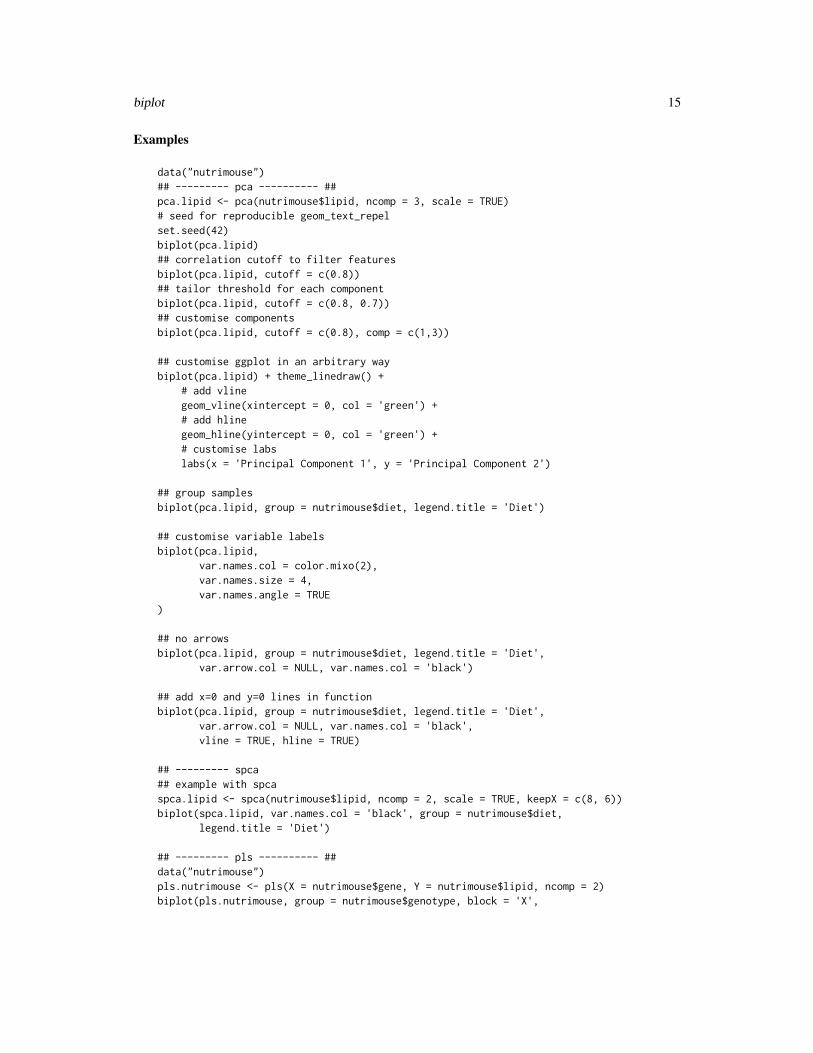
Examples

data("nutrimouse")## --------- pca ---------- ##pca.lipid <- pca(nutrimouse$lipid, ncomp = 3, scale = TRUE)# seed for reproducible geom_text_repelset.seed(42)biplot(pca.lipid)## correlation cutoff to filter featuresbiplot(pca.lipid, cutoff = c(0.8))## tailor threshold for each componentbiplot(pca.lipid, cutoff = c(0.8, 0.7))## customise componentsbiplot(pca.lipid, cutoff = c(0.8), comp = c(1,3))

## customise ggplot in an arbitrary waybiplot(pca.lipid) + theme_linedraw() +

# add vlinegeom_vline(xintercept = 0, col = 'green') +# add hlinegeom_hline(yintercept = 0, col = 'green') +# customise labslabs(x = 'Principal Component 1', y = 'Principal Component 2')

## group samplesbiplot(pca.lipid, group = nutrimouse$diet, legend.title = 'Diet')

## customise variable labelsbiplot(pca.lipid,

var.names.col = color.mixo(2),var.names.size = 4,var.names.angle = TRUE

)

## no arrowsbiplot(pca.lipid, group = nutrimouse$diet, legend.title = 'Diet',

var.arrow.col = NULL, var.names.col = 'black')

## add x=0 and y=0 lines in functionbiplot(pca.lipid, group = nutrimouse$diet, legend.title = 'Diet',

var.arrow.col = NULL, var.names.col = 'black',vline = TRUE, hline = TRUE)

## --------- spca## example with spcaspca.lipid <- spca(nutrimouse$lipid, ncomp = 2, scale = TRUE, keepX = c(8, 6))biplot(spca.lipid, var.names.col = 'black', group = nutrimouse$diet,

legend.title = 'Diet')

## --------- pls ---------- ##data("nutrimouse")pls.nutrimouse <- pls(X = nutrimouse$gene, Y = nutrimouse$lipid, ncomp = 2)biplot(pls.nutrimouse, group = nutrimouse$genotype, block = 'X',

16 block.pls

legend.title = 'Genotype', cutoff = 0.878)

biplot(pls.nutrimouse, group = nutrimouse$genotype, block = 'Y',legend.title = 'Genotype', cutoff = 0.8)

## --------- plsda ---------- ##data(breast.tumors)X <- breast.tumors$gene.expcolnames(X) <- paste0('GENE_', colnames(X))rownames(X) <- paste0('SAMPLE_', rownames(X))Y <- breast.tumors$sample$treatment

plsda.breast <- plsda(X, Y, ncomp = 2)biplot(plsda.breast, cutoff = 0.72)## remove arrowsbiplot(plsda.breast, cutoff = 0.72, var.arrow.col = NULL, var.names.size = 4)

block.pls N-integration with Projection to Latent Structures models (PLS)

Description

Integration of multiple data sets measured on the same samples or observations, ie. N-integration.The method is partly based on Generalised Canonical Correlation Analysis.

Usage

block.pls(X,Y,indY,ncomp = 2,design,scheme,mode,scale = TRUE,init,tol = 1e-06,max.iter = 100,near.zero.var = FALSE,all.outputs = TRUE

)

Arguments

X A named list of data sets (called ’blocks’) measured on the same samples. Datain the list should be arranged in matrices, samples x variables, with samplesorder matching in all data sets.

block.pls 17

Y Matrix response for a multivariate regression framework. Data should be con-tinuous variables (see ?block.plsda for supervised classification and factor re-sponse).

indY To supply if Y is missing, indicates the position of the matrix response in the listX.

ncomp the number of components to include in the model. Default to 2. Applies to allblocks.

design numeric matrix of size (number of blocks in X) x (number of blocks in X) withvalues between 0 and 1. Each value indicates the strenght of the relationship tobe modelled between two blocks; a value of 0 indicates no relationship, 1 is themaximum value. Alternatively, one of c(’null’, ’full’) indicating a disconnectedor fully connected design, respecively, or a numeric between 0 and 1 which willdesignate all off-diagonal elements of a fully connected design (see examples inblock.splsda). If Y is provided instead of indY, the design matrix is changedto include relationships to Y.

scheme Character, one of ’horst’, ’factorial’ or ’centroid’. Default = 'horst', see refer-ence.

mode Character string indicating the type of PLS algorithm to use. One of "regression","canonical", "invariant" or "classic". See Details.

scale Logical. If scale = TRUE, each block is standardized to zero means and unitvariances (default: TRUE)

init Mode of initialization use in the algorithm, either by Singular Value Decomposi-tion of the product of each block of X with Y (’svd’) or each block independently(’svd.single’). Default = svd.single.

tol Positive numeric used as convergence criteria/tolerance during the iterative pro-cess. Default to 1e-06.

max.iter Integer, the maximum number of iterations. Default to 100.

near.zero.var Logical, see the internal nearZeroVar function (should be set to TRUE in par-ticular for data with many zero values). Setting this argument to FALSE (whenappropriate) will speed up the computations. Default value is FALSE.

all.outputs Logical. Computation can be faster when some specific (and non-essential) out-puts are not calculated. Default = TRUE.

Details

block.spls function fits a horizontal integration PLS model with a specified number of compo-nents per block). An outcome needs to be provided, either by Y or by its position indY in the list ofblocks X. Multi (continuous)response are supported. X and Y can contain missing values. Missingvalues are handled by being disregarded during the cross product computations in the algorithmblock.pls without having to delete rows with missing data. Alternatively, missing data can beimputed prior using the impute.nipals function.

The type of algorithm to use is specified with the mode argument. Four PLS algorithms are available:PLS regression ("regression"), PLS canonical analysis ("canonical"), redundancy analysis("invariant") and the classical PLS algorithm ("classic") (see References and ?pls for moredetails).

18 block.pls

Note that our method is partly based on Generalised Canonical Correlation Analysis and differsfrom the MB-PLS approaches proposed by Kowalski et al., 1989, J Chemom 3(1) and Westerhuiset al., 1998, J Chemom, 12(5).

Value

block.pls returns an object of class 'block.pls', a list that contains the following components:

X the centered and standardized original predictor matrix.

indY the position of the outcome Y in the output list X.

ncomp the number of components included in the model for each block.

mode the algorithm used to fit the model.

variates list containing the variates of each block of X.

loadings list containing the estimated loadings for the variates.

names list containing the names to be used for individuals and variables.

nzv list containing the zero- or near-zero predictors information.

iter Number of iterations of the algorithm for each component

prop_expl_var Percentage of explained variance for each component and each block

Author(s)

Florian Rohart, Benoit Gautier, Kim-Anh Lê Cao, Al J Abadi

References

Tenenhaus, M. (1998). La regression PLS: theorie et pratique. Paris: Editions Technic.

Wold H. (1966). Estimation of principal components and related models by iterative least squares.In: Krishnaiah, P. R. (editors), Multivariate Analysis. Academic Press, N.Y., 391-420.

Tenenhaus A. and Tenenhaus M., (2011), Regularized Generalized Canonical Correlation Analysis,Psychometrika, Vol. 76, Nr 2, pp 257-284.

See Also

plotIndiv, plotArrow, plotLoadings, plotVar, predict, perf, selectVar, block.spls, block.plsdaand http://www.mixOmics.org for more details.

Examples

# Example with TCGA multi omics study# -----------------------------------data("breast.TCGA")# this is the X data as a list of mRNA and miRNA; the Y data set is a single data set of proteinsdata = list(mrna = breast.TCGA$data.train$mrna, mirna = breast.TCGA$data.train$mirna)# set up a full design where every block is connecteddesign = matrix(1, ncol = length(data), nrow = length(data),dimnames = list(names(data), names(data)))diag(design) = 0

block.plsda 19

design# set number of component per data setncomp = c(2)

TCGA.block.pls = block.pls(X = data, Y = breast.TCGA$data.train$protein,ncomp = ncomp, design = design)

TCGA.block.pls## use design = 'full'TCGA.block.pls = block.pls(X = data, Y = breast.TCGA$data.train$protein,

ncomp = ncomp, design = 'full')# in plotindiv we color the samples per breast subtype group but the method is unsupervised!# here Y is the protein data setplotIndiv(TCGA.block.pls, group = breast.TCGA$data.train$subtype, ind.names = FALSE)

block.plsda N-integration with Projection to Latent Structures models (PLS) withDiscriminant Analysis

Description

Integration of multiple data sets measured on the same samples or observations to classify a discreteoutcome, ie. N-integration with Discriminant Analysis. The method is partly based on GeneralisedCanonical Correlation Analysis.

Usage

block.plsda(X,Y,indY,ncomp = 2,design,scheme,scale = TRUE,init = "svd",tol = 1e-06,max.iter = 100,near.zero.var = FALSE,all.outputs = TRUE

)

Arguments


Y a factor or a class vector for the discrete outcome.

20 block.plsda











Details

block.plsda function fits a horizontal integration PLS-DA model with a specified number of com-ponents per block). A factor indicating the discrete outcome needs to be provided, either by Y or byits position indY in the list of blocks X.

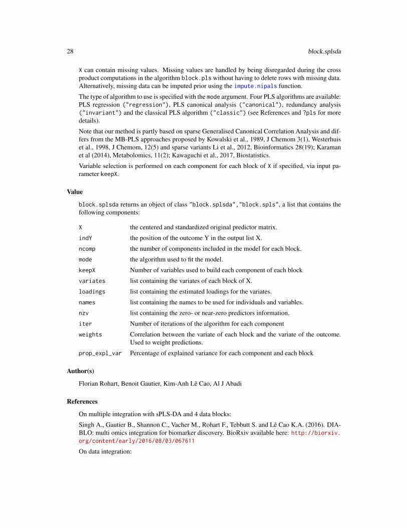
X can contain missing values. Missing values are handled by being disregarded during the crossproduct computations in the algorithm block.pls without having to delete rows with missing data.Alternatively, missing data can be imputed prior using the impute.nipals function.


Note that our method is partly based on Generalised Canonical Correlation Analysis and differsfrom the MB-PLS approaches proposed by Kowalski et al., 1989, J Chemom 3(1) and Westerhuiset al., 1998, J Chemom, 12(5).

block.plsda 21

Value

block.plsda returns an object of class "block.plsda","block.pls", a list that contains the fol-lowing components:











Author(s)


References

On PLSDA:

Barker M and Rayens W (2003). Partial least squares for discrimination. Journal of Chemometrics17(3), 166-173. Perez-Enciso, M. and Tenenhaus, M. (2003). Prediction of clinical outcome withmicroarray data: a partial least squares discriminant analysis (PLS-DA) approach. Human Genetics112, 581-592. Nguyen, D. V. and Rocke, D. M. (2002). Tumor classification by partial least squaresusing microarray gene expression data. Bioinformatics 18, 39-50.

On multiple integration with PLS-DA: Gunther O., Shin H., Ng R. T. , McMaster W. R., McManusB. M. , Keown P. A. , Tebbutt S.J. , Lê Cao K-A. , (2014) Novel multivariate methods for integrationof genomics and proteomics data: Applications in a kidney transplant rejection study, OMICS: Ajournal of integrative biology, 18(11), 682-95.

On multiple integration with sPLS-DA and 4 data blocks:

Singh A., Gautier B., Shannon C., Vacher M., Rohart F., Tebbutt S. and Lê Cao K.A. (2016). DIA-BLO: multi omics integration for biomarker discovery. BioRxiv available here: http://biorxiv.org/content/early/2016/08/03/067611

mixOmics article:


See Also

plotIndiv, plotArrow, plotLoadings, plotVar, predict, perf, selectVar, block.pls, block.splsdaand http://www.mixOmics.org for more details.

http://biorxiv.org/content/early/2016/08/03/067611


22 block.spls

Examples

data(nutrimouse)data = list(gene = nutrimouse$gene, lipid = nutrimouse$lipid, Y = nutrimouse$diet)# with this design, all blocks are connecteddesign = matrix(c(0,1,1,1,0,1,1,1,0), ncol = 3, nrow = 3,byrow = TRUE, dimnames = list(names(data), names(data)))

res = block.plsda(X = data, indY = 3) # indY indicates where the outcome Y is in the list XplotIndiv(res, ind.names = FALSE, legend = TRUE)plotVar(res)

## Not run:# when Y is providedres2 = block.plsda(list(gene = nutrimouse$gene, lipid = nutrimouse$lipid),Y = nutrimouse$diet, ncomp = 2)plotIndiv(res2)plotVar(res2)

## End(Not run)

block.spls N-integration and feature selection with sparse Projection to LatentStructures models (sPLS)

Description

Integration of multiple data sets measured on the same samples or observations, with variable se-lection in each data set, ie. N-integration. The method is partly based on Generalised CanonicalCorrelation Analysis.

Usage

block.spls(X,Y,indY,ncomp = 2,keepX,keepY,design,scheme,mode,scale = TRUE,init,tol = 1e-06,max.iter = 100,near.zero.var = FALSE,all.outputs = TRUE

)

block.spls 23

Arguments


Y Matrix response for a multivariate regression framework. Data should be con-tinuous variables (see ?block.splsda for supervised classification and factorresponse).



keepX A named list of same length as X. Each entry is the number of variables to selectin each of the blocks of X for each component. By default all variables are keptin the model.

keepY Only if Y is provided (and not indY). Each entry is the number of variables toselect in each of the blocks of Y for each component.










24 block.spls

Details

block.spls function fits a horizontal sPLS model with a specified number of components perblock). An outcome needs to be provided, either by Y or by its position indY in the list of blocks X.Multi (continuous)response are supported. X and Y can contain missing values. Missing values arehandled by being disregarded during the cross product computations in the algorithm block.plswithout having to delete rows with missing data. Alternatively, missing data can be imputed priorusing the nipals function.


Note that our method is partly based on sparse Generalised Canonical Correlation Analysis and dif-fers from the MB-PLS approaches proposed by Kowalski et al., 1989, J Chemom 3(1), Westerhuiset al., 1998, J Chemom, 12(5) and sparse variants Li et al., 2012, Bioinformatics 28(19); Karamanet al (2014), Metabolomics, 11(2); Kawaguchi et al., 2017, Biostatistics.

Variable selection is performed on each component for each block of X, and for Y if specified, viainput parameter keepX and keepY.

Note that if Y is missing and indY is provided, then variable selection on Y is performed by specify-ing the input parameter directly in keepX (no keepY is needed).

Value

block.spls returns an object of class "block.spls", a list that contains the following components:





keepX Number of variables used to build each component of each block

keepY Number of variables used to build each component of Y






prop_expl_var Percentage of explained variance for each component and each block after set-ting possible missing values in the centered data to zero

Author(s)


block.spls 25

References




Tenenhaus A., Philippe C., Guillemot V, Lê Cao K.A., Grill J, Frouin V. Variable selection forgeneralized canonical correlation analysis. Biostatistics. kxu001

See Also

plotIndiv, plotArrow, plotLoadings, plotVar, predict, perf, selectVar, block.pls, block.splsdaand http://www.mixOmics.org for more details.

Examples

# Example with multi omics TCGA study# -----------------------------data("breast.TCGA")# this is the X data as a list of mRNA and miRNA; the Y data set is a single data set of proteinsdata = list(mrna = breast.TCGA$data.train$mrna, mirna = breast.TCGA$data.train$mirna)# set up a full design where every block is connecteddesign = matrix(1, ncol = length(data), nrow = length(data),dimnames = list(names(data), names(data)))diag(design) = 0design# set number of component per data setncomp = c(2)# set number of variables to select, per component and per data set (this is set arbitrarily)list.keepX = list(mrna = rep(10, 2), mirna = rep(10,2))list.keepY = c(rep(10, 2))

TCGA.block.spls = block.spls(X = data, Y = breast.TCGA$data.train$protein,ncomp = ncomp, keepX = list.keepX, keepY = list.keepY, design = design)TCGA.block.spls# in plotindiv we color the samples per breast subtype group but the method is unsupervised!plotIndiv(TCGA.block.spls, group = breast.TCGA$data.train$subtype, ind.names = FALSE, legend=TRUE)# illustrates coefficient weights in each blockplotLoadings(TCGA.block.spls, ncomp = 1)plotVar(TCGA.block.spls, style = 'graphics', legend = TRUE)

## plot markers (selected markers) for mrna and mirnagroup <- breast.TCGA$data.train$subtype# mrna: show each selected feature separately and group by subtypeplotMarkers(object = TCGA.block.spls, comp = 1, block = 'mrna', group = group)# mrna: aggregate all selected features, separate by loadings signs and group by subtypeplotMarkers(object = TCGA.block.spls, comp = 1, block = 'mrna', group = group, global = TRUE)# proteinsplotMarkers(object = TCGA.block.spls, comp = 1, block = 'Y', group = group)## only show boxplots

26 block.splsda

plotMarkers(object = TCGA.block.spls, comp = 1, block = 'Y', group = group, violin = FALSE)

## Not run:network(TCGA.block.spls)

## End(Not run)

block.splsda N-integration and feature selection with Projection to Latent Struc-tures models (PLS) with sparse Discriminant Analysis

Description

Integration of multiple data sets measured on the same samples or observations to classify a discreteoutcome to classify a discrete outcome and select features from each data set, ie. N-integration withsparse Discriminant Analysis. The method is partly based on Generalised Canonical CorrelationAnalysis.

Usage

block.splsda(X,Y,indY,ncomp = 2,keepX,design,scheme,scale = TRUE,init = "svd",tol = 1e-06,max.iter = 100,near.zero.var = FALSE,all.outputs = TRUE

)

wrapper.sgccda(X,Y,indY,ncomp = 2,keepX,design,scheme,scale = TRUE,init = "svd",tol = 1e-06,

block.splsda 27

max.iter = 100,near.zero.var = FALSE,all.outputs = TRUE

)

Arguments


Y a factor or a class vector for the discrete outcome.indY To supply if Y is missing, indicates the position of the matrix response in the list

X.ncomp the number of components to include in the model. Default to 2. Applies to all

blocks.keepX A named list of same length as X. Each entry is the number of variables to select

in each of the blocks of X for each component. By default all variables are keptin the model.






max.iter Integer, the maximum number of iterations. Default to 100.near.zero.var Logical, see the internal nearZeroVar function (should be set to TRUE in par-

ticular for data with many zero values). Setting this argument to FALSE (whenappropriate) will speed up the computations. Default value is FALSE.


Details

block.splsda function fits a horizontal integration PLS-DA model with a specified number ofcomponents per block). A factor indicating the discrete outcome needs to be provided, either by Yor by its position indY in the list of blocks X.

28 block.splsda



Note that our method is partly based on sparse Generalised Canonical Correlation Analysis and dif-fers from the MB-PLS approaches proposed by Kowalski et al., 1989, J Chemom 3(1), Westerhuiset al., 1998, J Chemom, 12(5) and sparse variants Li et al., 2012, Bioinformatics 28(19); Karamanet al (2014), Metabolomics, 11(2); Kawaguchi et al., 2017, Biostatistics.

Variable selection is performed on each component for each block of X if specified, via input pa-rameter keepX.

Value

block.splsda returns an object of class "block.splsda","block.spls", a list that contains thefollowing components:





keepX Number of variables used to build each component of each block






weights Correlation between the variate of each block and the variate of the outcome.Used to weight predictions.


Author(s)


References

On multiple integration with sPLS-DA and 4 data blocks:


On data integration:



block.splsda 29


Gunther O., Shin H., Ng R. T. , McMaster W. R., McManus B. M. , Keown P. A. , Tebbutt S.J., Lê Cao K-A. , (2014) Novel multivariate methods for integration of genomics and proteomicsdata: Applications in a kidney transplant rejection study, OMICS: A journal of integrative biology,18(11), 682-95.

mixOmics article:


See Also

plotIndiv, plotArrow, plotLoadings, plotVar, predict, perf, selectVar, block.plsda, block.splsand http://www.mixOmics.org/mixDIABLO for more details and examples.

Examples

# block.splsda# -------------data("breast.TCGA")# this is the X data as a list of mRNA, miRNA and proteinsdata = list(mrna = breast.TCGA$data.train$mrna, mirna = breast.TCGA$data.train$mirna,protein = breast.TCGA$data.train$protein)# set up a full design where every block is connecteddesign = matrix(1, ncol = length(data), nrow = length(data),dimnames = list(names(data), names(data)))diag(design) = 0design# set number of component per data setncomp = c(2)# set number of variables to select, per component and per data set (this is set arbitrarily)list.keepX = list(mrna = rep(8,2), mirna = rep(8,2), protein = rep(8,2))

TCGA.block.splsda = block.splsda(X = data, Y = breast.TCGA$data.train$subtype,ncomp = ncomp, keepX = list.keepX, design = design)

## use design = 'full'TCGA.block.splsda = block.splsda(X = data, Y = breast.TCGA$data.train$subtype,

ncomp = ncomp, keepX = list.keepX, design = 'full')TCGA.block.splsda$design

plotIndiv(TCGA.block.splsda, ind.names = FALSE)## use design = 'null'TCGA.block.splsda = block.splsda(X = data, Y = breast.TCGA$data.train$subtype,

ncomp = ncomp, keepX = list.keepX, design = 'null')TCGA.block.splsda$design## set all off-diagonal elements to 0.5TCGA.block.splsda = block.splsda(X = data, Y = breast.TCGA$data.train$subtype,

ncomp = ncomp, keepX = list.keepX, design = 0.5)TCGA.block.splsda$design# illustrates coefficient weights in each block

30 breast.TCGA

plotLoadings(TCGA.block.splsda, ncomp = 1, contrib = 'max')plotVar(TCGA.block.splsda, style = 'graphics', legend = TRUE)

## plot markers (selected variables) for mrna and mirna# mrna: show each selected feature separatelyplotMarkers(object = TCGA.block.splsda, comp = 1, block = 'mrna')# mrna: aggregate all selected features and separate by loadings signsplotMarkers(object = TCGA.block.splsda, comp = 1, block = 'mrna', global = TRUE)# proteinsplotMarkers(object = TCGA.block.splsda, comp = 1, block = 'protein')## do not show violin plotsplotMarkers(object = TCGA.block.splsda, comp = 1, block = 'protein', violin = FALSE)# show top 5 markersplotMarkers(object = TCGA.block.splsda, comp = 1, block = 'protein', markers = 1:5)# show specific markersmy.markers <- selectVar(TCGA.block.splsda, comp = 1)[['protein']]$name[c(1,3,5)]my.markersplotMarkers(object = TCGA.block.splsda, comp = 1, block = 'protein', markers = my.markers)

breast.TCGA Breast Cancer multi omics data from TCGA

Description

This data set is a small subset of the full data set from The Cancer Genome Atlas that can be analysedwith the DIABLO framework. It contains the expression or abundance of three matching omics datasets: mRNA, miRNA and proteomics for 150 breast cancer samples (Basal, Her2, Luminal A) inthe training set, and 70 samples in the test set. The test set is missing the proteomics data set.

Usage

data(breast.TCGA)

Format

A list containing two data sets, data.train and data.test which both include:

list("miRNA") data frame with 150 (70) rows and 184 columns in the training (test) data set. Theexpression levels of 184 miRNA.

list("mRNA") data frame with 150 (70) rows and 520 columns in the training (test) data set. Theexpression levels of 200 mRNA.

list("protein") data frame with 150 (70) rows and 142 columns in the training data set only. Theabundance of 142 proteins.

list("subtype") a factor indicating the brerast cancer subtypes in the training (length of 150) andtest (length of 70) sets.

breast.tumors 31

Details

The data come from The Cancer Genome Atlas (TCGA, http://cancergenome.nih.gov/). We dividedthe data into a training (discovery) and test (validation) set. The protein dataset which had a limitednumber of subjects available was used to allocate subjects into the training set only, while the tesset included all remaining subject. Each data set was normalised and pre-processed. For illustrativepurposes we drastically filtered the data here.

Value

none

Source

The raw data were downloaded from http://cancergenome.nih.gov/. The normalised and fil-tered data we analysed with DIABLO are available on www.mixOmics.org/mixDIABLO

References

Singh A., Shannon C., Gautier B., Rohart F., Vacher M., Tebbutt S. and Lê Cao K.A. (2019),DIABLO: an integrative approach for identifying key molecular drivers from multi-omics assays,Bioinformatics, Volume 35, Issue 17, 1 September 2019, Pages 3055–3062.

breast.tumors Human Breast Tumors Data

Description

This data set contains the expression of 1,000 genes in 47 surgical specimens of human breasttumours from 17 different individuals before and after chemotherapy treatment.

Usage

data(breast.tumors)

Format

A list containing the following components:

list("gene.exp") data matrix with 47 rows and 1000 columns. Each row represents an experimentalsample, and each column a single gene.

list("sample") a list containing two character vector components: name the name of the samples,and treatment the treatment status.

list("genes") a list containing two character vector components: name the name of the genes, anddescription the description of each gene.

http://cancergenome.nih.gov/

www.mixOmics.org/mixDIABLO

32 cim

Details

This data consists of 47 breast cancer samples and 1753 cDNA clones pre-selected by Perez-Encisoet al. (2003) to draw their Fig. 1. The authors selected 47 samples for which there was informa-tion at least before or before and after chemotherapy treatment. There were 20 tumours that weremicroarrayed both before and after treatment. For illustrative purposes we then randomly selected1000 cDNA clones for this data set.

Value

none

Source

The Human Breast Tumors dataset is a companion resource for the paper of Perou et al. (2000), andwas downloaded from the Stanford Genomics Breast Cancer Consortium Portal http://genome-www.stanford.edu/breast_cancer/molecularportraits/download.shtml

References

Perez-Enciso, M. and Tenenhaus, M. (2003). Prediction of clinical outcome with microarray data:a partial least squares discriminant analysis (PLS-DA) approach. Human Genetics 112, 581-592.

Perou, C. M., Sorlie, T., Eisen, M. B., van de Rijn, M., Jeffrey, S. S., Rees, C. A., Pollack, J. R.,Ross, D. T., Johnsen, H., Akslen, L. A., Fluge, O., Pergamenschikov, A., Williams, C., Zhu, S. X.,Lonning, P. E., Borresen-Dale, A. L., Brown, P. O. and Botstein, D. (2000). Molecular portraits ofhuman breast tumours. Nature 406, 747-752.

cim Clustered Image Maps (CIMs) ("heat maps")

Description

This function generates color-coded Clustered Image Maps (CIMs) ("heat maps") to represent"high-dimensional" data sets.

Usage

cim(mat = NULL,color = NULL,row.names = TRUE,col.names = TRUE,row.sideColors = NULL,col.sideColors = NULL,row.cex = NULL,col.cex = NULL,cutoff = 0,cluster = "both",

http://genome-www.stanford.edu/breast_cancer/molecularportraits/download.shtml

http://genome-www.stanford.edu/breast_cancer/molecularportraits/download.shtml

cim 33

dist.method = c("euclidean", "euclidean"),clust.method = c("complete", "complete"),cut.tree = c(0, 0),transpose = FALSE,symkey = TRUE,keysize = c(1, 1),keysize.label = 1,zoom = FALSE,title = NULL,xlab = NULL,ylab = NULL,margins = c(5, 5),lhei = NULL,lwid = NULL,comp = NULL,center = TRUE,scale = FALSE,mapping = "XY",legend = NULL,save = NULL,name.save = NULL

)

Arguments

mat numeric matrix of values to be plotted. Alternatively, an object of class inher-iting from "pca", "spca", "ipca", "sipca", "rcc", "pls", "spls", "plsda","splsda", "mlspls" or "mlsplsda" (where "ml" stands for multilevel).

color a character vector of colors such as that generated by terrain.colors, topo.colors,rainbow, color.jet or similar functions.

row.names, col.names

logical, should the name of rows and/or columns of mat be shown? If TRUE(defaults) rownames(mat) and/or colnames(mat) are used. Possible charactervectors with row and/or column labels can be used.

row.sideColors (optional) character vector of length nrow(mat) containing the color names fora vertical side bar that may be used to annotate the rows of mat.

col.sideColors (optional) character vector of length ncol(mat) containing the color names fora horizontal side bar that may be used to annotate the columns of mat.

row.cex, col.cex

positive numbers, used as cex.axis in for the row or column axis labeling. Thedefaults currently only use number of rows or columns, respectively.

cutoff numeric between 0 and 1. Variables with correlations below this threshold inabsolute value are not plotted. To use only when mapping is "XY".

cluster character string indicating whether to cluster "none", "row", "column" or "both".Defaults to "both".

dist.method character vector of length two. The distance measure used in clustering rowsand columns. Possible values are "correlation" for Pearson correlation andall the distances supported by dist, such as "euclidean", etc.

34 cim

clust.method character vector of length two. The agglomeration method to be used for rowsand columns. Accepts the same values as in hclust such as "ward", "complete",etc.

cut.tree numeric vector of length two with components in [0,1]. The height proportionswhere the trees should be cut for rows and columns, if these are clustered.

transpose logical indicating if the matrix should be transposed for plotting. Defaults toFALSE.

symkey Logical indicating whether the color key should be made symmetric about 0.Defaults to TRUE.

keysize vector of length two, indicating the size of the color key.

keysize.label vector of length 1, indicating the size of the labels and title of the color key.

zoom logical. Whether to use zoom for interactive zoom. See Details.title, xlab, ylab

title, x- and y-axis titles; default to none.

margins numeric vector of length two containing the margins (see par(mar)) for columnand row names respectively.

lhei, lwid arguments passed to layout to divide the device up into two (or three if aside color is drawn) rows and two columns, with the row-heights lhei and thecolumn-widths lwid.

comp atomic or vector of positive integers. The components to adequately accountfor the data association. For a non sparse method, the similarity matrix is com-puted based on the variates and loading vectors of those specified components.For a sparse approach, the similarity matric is computed based on the vari-ables selected on those specified components. See example. Defaults to comp =1:object$ncomp.

center either a logical value or a numeric vector of length equal to the number ofcolumns of mat. See scale function.

scale either a logical value or a numeric vector of length equal to the number ofcolumns of mat. See scale function.

mapping character string indicating whether to map "X", "Y" or "XY"-association matrix.See Details.

legend A list indicating the legend for each group, the color vector, title of the legendand cex.

save should the plot be saved? If so, argument to be set to either 'jpeg', 'tiff','png' or 'pdf'.

name.save character string for the name of the file to be saved.

Details

One matrix Clustered Image Map (default method) is a 2-dimensional visualization of a real-valuedmatrix (basically image(t(mat))) with rows and/or columns reordered according to some hierar-chical clustering method to identify interesting patterns. Generated dendrograms from clusteringare added to the left side and to the top of the image. By default the used clustering method for

cim 35

rows and columns is the complete linkage method and the used distance measure is the distanceeuclidean.

In "pca", "spca", "ipca", "sipca", "plsda", "splsda" and multilevel variants methods the matmatrix is object$X.

For the remaining methods, if mapping = "X" or mapping = "Y" the mat matrix is object$X orobject$Y respectively. If mapping = "XY":

• in rcc method, the matrix mat is created where element (j, k) is the scalar product valuebetween every pairs of vectors in dimension length(comp) representing the variables Xj andYk on the axis defined by Zi with i in comp, where Zi is the equiangular vector between thei-th X and Y canonical variate.

• in pls, spls and multilevel spls methods, if object$mode is "regression", the element(j, k) of the matrix mat is given by the scalar product value between every pairs of vectorsin dimension length(comp) representing the variables Xj and Yk on the axis defined by Ui

with i in comp, where Ui is the i-th X variate. If object$mode is "canonical" then Xj andYk are represented on the axis defined by Ui and Vi respectively.

By default four components will be displayed in the plot. At the top left is the color key, top rightis the column dendogram, bottom left is the row dendogram, bottom right is the image plot. WhensideColors are provided, an additional row or column is inserted in the appropriate location. Thislayout can be overriden by specifiying appropriate values for lwid and lhei. lwid controls thecolumn width, and lhei controls the row height. See the help page for layout for details on howto use these arguments.

For visualization of "high-dimensional" data sets, a nice zooming tool was created. zoom = TRUEopen a new device, one for CIM, one for zoom-out region and define an interactive ’zoom’ process:click two points at imagen map region by pressing the first mouse button. It then draws a rectanglearound the selected region and zoom-out this at new device. The process can be repeated to zoom-out other regions of interest.

The zoom process is terminated by clicking the second button and selecting ’Stop’ from the menu,or from the ’Stop’ menu on the graphics window.

Value


M the mapped matrix used by cim.

rowInd, colInd row and column index permutation vectors as returned by order.dendrogram.

ddr, ddc object of class "dendrogram" which describes the row and column trees pro-duced by cim.

mat.cor the correlation matrix used for the heatmap. Available only when mapping ="XY".


character vectors with row and column labels used.row.sideColors, col.sideColors

character vector containing the color names for vertical and horizontal side barsused to annotate the rows and columns.

36 cim

Author(s)

Ignacio González, Francois Bartolo, Kim-Anh Lê Cao, Al J Abadi

References

Eisen, M. B., Spellman, P. T., Brown, P. O. and Botstein, D. (1998). Cluster analysis and display ofgenome-wide expression patterns. Proceeding of the National Academy of Sciences of the USA 95,14863-14868.

Weinstein, J. N., Myers, T. G., O’Connor, P. M., Friend, S. H., Fornace Jr., A. J., Kohn, K. W.,Fojo, T., Bates, S. E., Rubinstein, L. V., Anderson, N. L., Buolamwini, J. K., van Osdol, W. W.,Monks, A. P., Scudiero, D. A., Sausville, E. A., Zaharevitz, D. W., Bunow, B., Viswanadhan, V.N., Johnson, G. S., Wittes, R. E. and Paull, K. D. (1997). An information-intensive approach to themolecular pharmacology of cancer. Science 275, 343-349.

González I., Lê Cao K.A., Davis M.J., Déjean S. (2012). Visualising associations between paired’omics’ data sets. BioData Mining; 5(1).

mixOmics article:


See Also

heatmap, hclust, plotVar, network and

http://mixomics.org/graphics/ for more details on all options available.

Examples

## default method: shows cross correlation between 2 data sets#------------------------------------------------------------------data(nutrimouse)X <- nutrimouse$lipidY <- nutrimouse$gene

cim(cor(X, Y), cluster = "none")

## Not run:## CIM representation for objects of class 'rcc'#------------------------------------------------------------------

nutri.rcc <- rcc(X, Y, ncomp = 3, lambda1 = 0.064, lambda2 = 0.008)

cim(nutri.rcc, xlab = "genes", ylab = "lipids", margins = c(5, 6))

#-- interactive 'zoom' available as below

cim(nutri.rcc, xlab = "genes", ylab = "lipids", margins = c(5, 6),zoom = TRUE)#-- select the region and "see" the zoom-out region

http://mixomics.org/graphics/

cim 37

#-- cim from X matrix with a side bar to indicate the dietdiet.col <- palette()[as.numeric(nutrimouse$diet)]cim(nutri.rcc, mapping = "X", row.names = nutrimouse$diet,row.sideColors = diet.col, xlab = "lipids",clust.method = c("ward", "ward"), margins = c(6, 4))

#-- cim from Y matrix with a side bar to indicate the genotypegeno.col = color.mixo(as.numeric(nutrimouse$genotype))cim(nutri.rcc, mapping = "Y", row.names = nutrimouse$genotype,row.sideColors = geno.col, xlab = "genes",clust.method = c("ward", "ward"))

#-- save the result as a jpeg filejpeg(filename = "test.jpeg", res = 600, width = 4000, height = 4000)cim(nutri.rcc, xlab = "genes", ylab = "lipids", margins = c(5, 6))dev.off()

## CIM representation for objects of class 'spca' (also works for sipca)#------------------------------------------------------------------

data(liver.toxicity)X <- liver.toxicity$gene

liver.spca <- spca(X, ncomp = 2, keepX = c(30, 30), scale = FALSE)

dose.col <- color.mixo(as.numeric(as.factor(liver.toxicity$treatment[, 3])))

# side bar, no variable names showncim(liver.spca, row.sideColors = dose.col, col.names = FALSE,row.names = liver.toxicity$treatment[, 3],clust.method = c("ward", "ward"))

## CIM representation for objects of class '(s)pls'#------------------------------------------------------------------

data(liver.toxicity)

X <- liver.toxicity$geneY <- liver.toxicity$clinicliver.spls <- spls(X, Y, ncomp = 3,keepX = c(20, 50, 50), keepY = c(10, 10, 10))

# defaultcim(liver.spls)

# transpose matrix, choose clustering methodcim(liver.spls, transpose = TRUE,clust.method = c("ward", "ward"), margins = c(5, 7))

38 cim

# Here we visualise only the X variables selectedcim(liver.spls, mapping="X")

# Here we should visualise only the Y variables selectedcim(liver.spls, mapping="Y")

# Here we only visualise the similarity matrix between the variables by splscim(liver.spls, cluster="none")

# plotting two data sets with the similarity matrix as input in the funciton# (see our BioData Mining paper for more details)# Only the variables selected by the sPLS model in X and Y are representedcim(liver.spls, mapping="XY")

# on the X matrix only, side col var to indicate dosedose.col <- color.mixo(as.numeric(as.factor(liver.toxicity$treatment[, 3])))cim(liver.spls, mapping = "X", row.sideColors = dose.col,row.names = liver.toxicity$treatment[, 3])

# CIM default representation includes the total of 120 genes selected, with the dose color# with a sparse method, show only the variables selected on specific componentscim(liver.spls, comp = 1)cim(liver.spls, comp = 2)cim(liver.spls, comp = c(1,2))cim(liver.spls, comp = c(1,3))

## CIM representation for objects of class '(s)plsda'#------------------------------------------------------------------data(liver.toxicity)

X <- liver.toxicity$gene# Setting up the Y outcome firstY <- liver.toxicity$treatment[, 3]#set up colors for cimdose.col <- color.mixo(as.numeric(as.factor(liver.toxicity$treatment[, 3])))

liver.splsda <- splsda(X, Y, ncomp = 2, keepX = c(40, 30))

cim(liver.splsda, row.sideColors = dose.col, row.names = Y)

## CIM representation for objects of class splsda 'multilevel'# with a two level factor (repeated sample and time)#------------------------------------------------------------------data(vac18.simulated)X <- vac18.simulated$genesdesign <- data.frame(samp = vac18.simulated$sample)Y = data.frame(time = vac18.simulated$time,stim = vac18.simulated$stimulation)

res.2level <- splsda(X, Y = Y, ncomp = 2, multilevel = design,

cim 39

keepX = c(120, 10))

#define colors for the levels: stimulation and timestim.col <- c("darkblue", "purple", "green4","red3")stim.col <- stim.col[as.numeric(Y$stim)]time.col <- c("orange", "cyan")[as.numeric(Y$time)]

# The row side bar indicates the two levels of the facteor, stimulation and time.# the sample names have been motified on the plot.cim(res.2level, row.sideColors = cbind(stim.col, time.col),row.names = paste(Y$time, Y$stim, sep = "_"),col.names = FALSE,#setting up legend:legend=list(legend = c(levels(Y$time), levels(Y$stim)),col = c("orange", "cyan", "darkblue", "purple", "green4","red3"),title = "Condition", cex = 0.7))

## CIM representation for objects of class spls 'multilevel'#------------------------------------------------------------------

data(liver.toxicity)repeat.indiv <- c(1, 2, 1, 2, 1, 2, 1, 2, 3, 3, 4, 3, 4, 3, 4, 4, 5, 6, 5, 5,6, 5, 6, 7, 7, 8, 6, 7, 8, 7, 8, 8, 9, 10, 9, 10, 11, 9, 9,10, 11, 12, 12, 10, 11, 12, 11, 12, 13, 14, 13, 14, 13, 14,13, 14, 15, 16, 15, 16, 15, 16, 15, 16)

# sPLS is a non supervised technique, and so we only indicate the sample repetitions# in the design (1 factor only here, sample)# sPLS takes as an input 2 data sets, and the variables selecteddesign <- data.frame(sample = repeat.indiv)res.spls.1level <- spls(X = liver.toxicity$gene,Y=liver.toxicity$clinic,multilevel = design,ncomp = 2,keepX = c(50, 50), keepY = c(5, 5),mode = 'canonical')

stim.col <- c("darkblue", "purple", "green4","red3")

# showing only the Y variables, and only those selected in comp 1cim(res.spls.1level, mapping="Y",row.sideColors = stim.col[factor(liver.toxicity$treatment[,3])], comp = 1,#setting up legend:legend=list(legend = unique(liver.toxicity$treatment[,3]), col=stim.col,title = "Dose", cex=0.9))

# showing only the X variables, for all selected on comp 1 and 2cim(res.spls.1level, mapping="X",row.sideColors = stim.col[factor(liver.toxicity$treatment[,3])],#setting up legend:

40 cimDiablo

legend=list(legend = unique(liver.toxicity$treatment[,3]), col=stim.col,title = "Dose", cex=0.9))

# These are the cross correlations between the variables selected in X and Y.# The similarity matrix is obtained as in our paper in Data Miningcim(res.spls.1level, mapping="XY")

## End(Not run)

cimDiablo Clustered Image Maps (CIMs) ("heat maps") for DIABLO

Description

This function generates color-coded Clustered Image Maps (CIMs) ("heat maps") to represent"high-dimensional" data sets analysed with DIABLO.

Usage

cimDiablo(object,color = NULL,color.Y,color.blocks,comp = NULL,margins = c(2, 15),legend.position = "topright",transpose = FALSE,row.names = TRUE,col.names = TRUE,size.legend = 1.5,trim = TRUE,...

)

Arguments

object An object of class inheriting from "block.splsda".

color a character vector of colors such as that generated by terrain.colors, topo.colors,rainbow, color.jet or similar functions.

color.Y a character vector of colors to be used for the levels of the outcome

color.blocks a character vector of colors to be used for the blocks

comp positive integer. The similarity matrix is computed based on the variables se-lected on those specified components. See example. Defaults to comp = 1.

cimDiablo 41


legend.position

position of the legend, one of "bottomright", "bottom", "bottomleft", "left","topleft", "top", "topright", "right" and "center".

transpose logical indicating if the matrix should be transposed for plotting. Defaults toFALSE.


logical, should the name of rows and/or columns of mat be shown? If TRUE(defaults) rownames(mat) and/or colnames(mat) are used. Possible charactervectors with row and/or column labels can be used.

size.legend size of the legend

trim (Logical or numeric) If FALSE, values are not changed. If TRUE, the values aretrimmed to 3 standard deviation range. If a numeric, values with absolute valuesgreater than the provided values are trimmed.

... Other valid arguments passed to cim.

Details

This function is a small wrapper of cim specific to the DIABLO framework.

Value


M the mapped matrix used by cim.

rowInd, colInd row and column index permutation vectors as returned by order.dendrogram.

ddr, ddc object of class "dendrogram" which describes the row and column trees pro-duced by cim.

mat.cor the correlation matrix used for the heatmap. Available only when mapping ="XY".


character vectors with row and column labels used.row.sideColors, col.sideColors

character vector containing the color names for vertical and horizontal side barsused to annotate the rows and columns.

Author(s)

Amrit Singh, Florian Rohart, Kim-Anh Lê Cao, Al J Abadi

References


42 circosPlot

Eisen, M. B., Spellman, P. T., Brown, P. O. and Botstein, D. (1998). Cluster analysis and display ofgenome-wide expression patterns. Proceeding of the National Academy of Sciences of the USA 95,14863-14868.

Weinstein, J. N., Myers, T. G., O’Connor, P. M., Friend, S. H., Fornace Jr., A. J., Kohn, K. W.,Fojo, T., Bates, S. E., Rubinstein, L. V., Anderson, N. L., Buolamwini, J. K., van Osdol, W. W.,Monks, A. P., Scudiero, D. A., Sausville, E. A., Zaharevitz, D. W., Bunow, B., Viswanadhan, V.N., Johnson, G. S., Wittes, R. E. and Paull, K. D. (1997). An information-intensive approach to themolecular pharmacology of cancer. Science 275, 343-349.


mixOmics article:


See Also

cim, heatmap, hclust, plotVar, network and

http://mixomics.org/mixDIABLO/ for more details on all options available.

Examples

## default method: shows cross correlation between 2 data sets#------------------------------------------------------------------data(nutrimouse)Y = nutrimouse$dietdata = list(gene = nutrimouse$gene, lipid = nutrimouse$lipid)

nutrimouse.sgccda <- block.splsda(X = data,Y = Y,design = "full",keepX = list(gene = c(10,10), lipid = c(15,15)),ncomp = 2,scheme = "centroid")

cimDiablo(nutrimouse.sgccda, comp = c(1,2))## change trim rangecimDiablo(nutrimouse.sgccda, comp = c(1,2), trim = 4)## do not trim valuescimDiablo(nutrimouse.sgccda, comp = c(1,2), trim = FALSE)

circosPlot circosPlot for DIABLO

Description

Displays variable correlation among different blocks

http://mixomics.org/mixDIABLO/

circosPlot 43

Usage

## S3 method for class 'block.splsda'circosPlot(object,comp = 1:min(object$ncomp),cutoff,color.Y,blocks = NULL,color.blocks,color.cor,var.names = NULL,showIntraLinks = FALSE,line = FALSE,size.legend = 0.8,ncol.legend = 1,size.variables = 0.25,size.labels = 1,legend = TRUE,linkWidth = 1,...

)

## S3 method for class 'block.spls'circosPlot(object, ..., group = NULL, Y.name = "Y")

Arguments

object An object of class inheriting from "block.splsda" or "blocks.spls".

comp Numeric vector indicating which component to plot. Default to all

cutoff Only shows links with a correlation higher than cutoff

color.Y a character vector of colors to be used for the levels of the outcome

blocks Character or integer vector indicating which blocks to show. Default to all

color.blocks a character vector of colors to be used for the blocks

color.cor a character vector of two colors. First one is for the negative correlation, secondone is for the positive correlation

var.names Optional parameter. A list of length the number of blocks in object$X, contain-ing the names of the variables of each block. If NULL, the colnames of the datamatrix are used.

showIntraLinks if TRUE, shows the correlation higher than the threshold inside each block.

line if TRUE, shows the overall expression of the selected variables. see examples.

size.legend size of the legend

ncol.legend number of columns for the legend

size.variables size of the variable labels

size.labels size of the block labels

44 circosPlot

legend Logical. Whether the legend should be added. Default is TRUE.

linkWidth Numeric. Specifies the range of sizes used for lines linking the correlated vari-ables (see details). Must be of length 2 or 1. Default to c(1). See details.

... For object of class block.splsda, advanced plot parameters:

• var.adj Numeric. Adjusts the radial location of variable names in units ofthe arc band width. Positive values push feature names radially outward.Default to -0.33. See examples.

• block.labels.adj Numeric between -1 and 1. Adjusts the radial location ofblock names radially inward or outward. Default to 0. See examples.

• blocks.link Character vector of blocks. If provided, only correlations fromfeatures of these blocks are shown using links. See examples.

For object of class block.spls, all listed and advanced arguments passed to theblock.splsda method.

group The grouping factor used when line = TRUE

Y.name Character, the name of the Y block

Details

circosPlot function depicts correlations of variables selected with block.splsda or block.splsamong different blocks, using a generalisation of the method presented in González et al 2012. Ifncomp is specified, then only the variables selected on that component are displayed.

The linkWidth argument specifies the width of the links drawn. If a vector of length 2 is provided,the smaller value will correspond to a similarity values designated by cutoff argument, while thelarger value will be used for a link with perfect similarity (1), if any.

Value

If saved in an object, the circos plot will output the similarity matrix and the names of the variablesdisplayed on the plot (see attributes(object)).

Author(s)

Michael Vacher, Amrit Singh, Florian Rohart, Kim-Anh Lê Cao, Al J Abadi

References


mixOmics article:





circosPlot 45

See Also

block.splsda, references and http://www.mixOmics.org/mixDIABLO for more details.

Examples

data(nutrimouse)Y = nutrimouse$dietdata = list(gene = nutrimouse$gene, lipid = nutrimouse$lipid)design = matrix(c(0,1,1,1,0,1,1,1,0), ncol = 3, nrow = 3, byrow = TRUE)

nutrimouse.sgccda <- wrapper.sgccda(X=data,Y = Y,design = design,keepX = list(gene=c(10,10), lipid=c(15,15)),ncomp = 2,scheme = "horst")

circosPlot(nutrimouse.sgccda, cutoff = 0.7)## links widths based on strength of their similaritycircosPlot(nutrimouse.sgccda, cutoff = 0.7, linkWidth = c(1, 10))## custom legendcircosPlot(nutrimouse.sgccda, cutoff = 0.7, size.legend = 1.1)

## more customisationcircosPlot(nutrimouse.sgccda, cutoff = 0.7, size.legend = 1.1, color.Y = 1:5,

color.blocks = c("green","brown"), color.cor = c("magenta", "purple"))

par(mfrow=c(2,2))

circosPlot(nutrimouse.sgccda, cutoff = 0.7, size.legend = 1.1)## also show intra-block correlationscircosPlot(nutrimouse.sgccda, cutoff = 0.7,

size.legend = 1.1, showIntraLinks = TRUE)## show linescircosPlot(nutrimouse.sgccda, cutoff = 0.7, line = TRUE, ncol.legend = 1,

size.legend = 1.1, showIntraLinks = TRUE)## custom line legendscircosPlot(nutrimouse.sgccda, cutoff = 0.7, line = TRUE, ncol.legend = 2,

size.legend = 1.1, showIntraLinks = TRUE)par(mfrow=c(1,1))

## adjust feature and block names radiallycircosPlot(nutrimouse.sgccda, cutoff = 0.7, size.legend = 1.1)circosPlot(nutrimouse.sgccda, cutoff = 0.7, size.legend = 1.1,

var.adj = 0.8, block.labels.adj = -0.5)## --- example using breast.TCGA datadata("breast.TCGA")data = list(mrna = breast.TCGA$data.train$mrna,

mirna = breast.TCGA$data.train$mirna,protein = breast.TCGA$data.train$protein)

list.keepX = list(mrna = rep(20, 2), mirna = rep(10,2), protein = c(10, 2))

46 colors

TCGA.block.splsda = block.splsda(X = data,Y =breast.TCGA$data.train$subtype,ncomp = 2, keepX = list.keepX,design = 'full')

circosPlot(TCGA.block.splsda, cutoff = 0.7, line=TRUE)## show only first 2 blockscircosPlot(TCGA.block.splsda, cutoff = 0.7, line=TRUE, blocks = c(1,2))## show only correlations including the mrna block featurescircosPlot(TCGA.block.splsda, cutoff = 0.7, blocks.link = 'mrna')

data("breast.TCGA")data = list(mrna = breast.TCGA$data.train$mrna, mirna = breast.TCGA$data.train$mirna)list.keepX = list(mrna = rep(20, 2), mirna = rep(10,2))list.keepY = c(rep(10, 2))

TCGA.block.spls = block.spls(X = data,Y = breast.TCGA$data.train$protein,ncomp = 2, keepX = list.keepX,keepY = list.keepY, design = 'full')

circosPlot(TCGA.block.spls, group = breast.TCGA$data.train$subtype, cutoff = 0.7,Y.name = 'protein')

## only show links including mrnacircosPlot(TCGA.block.spls, group = breast.TCGA$data.train$subtype, cutoff = 0.7,

Y.name = 'protein', blocks.link = 'mrna')

colors Color Palette for mixOmics

Description

The functions create a vector of n "contiguous" colors (except the color.mixo which are colorsused internally to fit our logo colors).

Usage

color.mixo(num.vector)

color.GreenRed(n, alpha = 1)

color.jet(n, alpha = 1)

color.spectral(n, alpha = 1)

Arguments

num.vector for color.mixo an integer vector specifying which colors to use in the mixOmicspalette (there are only 10 colors available.

colors 47

n an integer, the number of colors (≥ 1) to be in the palette.

alpha a numeric value between 0 and 1 for alpha channel (opacity).

Details

The function color.jet(n) create color scheme, beginning with dark blue, ranging through shadesof blue, cyan, green, yellow and red, and ending with dark red. This colors palette is suitable fordisplaying ordered (symmetric) data, with n giving the number of colors desired.

Value

For color.jet(n), color.spectral(n), color.GreenRed(n) a character vector, cv, of colornames. This can be used either to create a user-defined color palette for subsequent graphics bypalette(cv), a col= specification in graphics functions or in par.

For color.mixo, a vector of colors matching the mixOmics logo (10 colors max.)

Author(s)

Ignacio Gonzalez, Kim-Anh Lê Cao, Benoit Gautier, Al J Abadi

See Also

colorRamp, palette, colors for the vector of built-in "named" colors; hsv, gray, rainbow,terrain.colors, ... to construct colors; and heat.colors, topo.colors for images.

Examples

# -----------------------# jet colors# ----------------------par(mfrow = c(3, 1))z <- seq(-1, 1, length = 125)for (n in c(11, 33, 125)) {image(matrix(z, ncol = 1), col = color.jet(n),xaxt = 'n', yaxt = 'n', main = paste('n = ', n))box()par(usr = c(-1, 1, -1, 1))axis(1, at = c(-1, 0, 1))}

## Not run:# -----------------------# spectral colors# ----------------------par(mfrow = c(3, 1))z <- seq(-1, 1, length = 125)for (n in c(11, 33, 125)) {image(matrix(z, ncol = 1), col = color.spectral(n),xaxt = 'n', yaxt = 'n', main = paste('n = ', n))box()par(usr = c(-1, 1, -1, 1))

48 diverse.16S

axis(1, at = c(-1, 0, 1))}

# -----------------------# GreenRed colors# ----------------------par(mfrow = c(3, 1))z <- seq(-1, 1, length = 125)for (n in c(11, 33, 125)) {image(matrix(z, ncol = 1), col = color.GreenRed(n),xaxt = 'n', yaxt = 'n', main = paste('n = ', n))box()par(usr = c(-1, 1, -1, 1))axis(1, at = c(-1, 0, 1))}

# # --------------------------------# mixOmics colors# # -------------------------------data(nutrimouse)X <- nutrimouse$lipidY <- nutrimouse$genenutri.res <- rcc(X, Y, ncomp = 3, lambda1 = 0.064, lambda2 = 0.008)

my.colors = color.mixo(1:5)my.pch = ifelse(nutrimouse$genotype == 'wt', 16, 17)#plotIndiv(nutri.res, ind.names = FALSE, group = my.colors, pch = my.pch, cex = 1.5)

## End(Not run)

diverse.16S 16S microbiome data: most diverse bodysites from HMP

Description

The 16S data from the Human Microbiome Project includes only the most diverse bodysites: An-tecubital fossa (skin), Stool and Subgingival plaque (oral) and can be analysed using a multilevelapproach to account for repeated measurements using our module mixMC. The data include 162samples (54 unique healthy individuals) measured on 1,674 OTUs.

Usage

data(diverse.16S)

Format

A list containing two data sets, data.TSS and data.raw and some meta data information:

list("data.TSS") data frame with 162 rows (samples) and 1674 columns (OTUs). The prefilterednormalised data using Total Sum Scaling normalisation.

estim.regul 49

list("data.raw") data frame with 162 rows (samples) and 1674 columns (OTUs). The prefilteredraw count OTU data which include a 1 offset (i.e. no 0 values).

list("taxonomy") data frame with 1674 rows (OTUs) and 6 columns indicating the taxonomy ofeach OTU.

list("indiv") data frame with 162 rows indicating sample meta data.

list("bodysite") factor of length 162 indicating the bodysite with levels "Antecubital_fossa", "Stool"and "Subgingival_plaque".

list("sample") vector of length 162 indicating the unique individual ID, useful for a multilevelapproach to taken into account the repeated measured on each individual.

Details

The data were downloaded from the Human Microbiome Project (HMP, http://hmpdacc.org/HMQCP/all/for the V1-3 variable region). The original data contained 43,146 OTU counts for 2,911 samplesmeasured from 18 different body sites. We focused on the first visit of each healthy individual andfocused on the three most diverse habitats. The prefiltered dataset included 1,674 OTU counts. Westrongly recommend to use log ratio transformations on the data.TSS normalised data, as imple-mented in the PLS and PCA methods, see details on www.mixOmics.org/mixMC.

The data.raw include a 1 offset in order to be log ratios transformed after TSS normalisation.Consequently, the data.TSS are TSS normalisation of data.raw. The CSS normalisation wasperformed on the orignal data (including zero values)

Value

none

Source

The raw data were downloaded from http://hmpdacc.org/HMQCP/all/. Filtering and normalisa-tion described in our website www.mixOmics.org/mixMC

References

Lê Cao K.-A., Costello ME, Lakis VA, Bartolo, F,Chua XY, Brazeilles R, Rondeau P. MixMC:Multivariate insights into Microbial Communities. PLoS ONE, 11(8): e0160169 (2016).

estim.regul Estimate the parameters of regularization for Regularized CCA

Description

This function has been renamed tune.rcc, see tune.rcc.

This function has been renamed ’image.tune.rcc’, see image.tune.rcc.

This function has been renamed tune.pca.

www.mixOmics.org/mixMC

http://hmpdacc.org/HMQCP/all/


50 explained_variance

Value

none

none

none

explained_variance Calculates the proportion of explained variance of multivariate com-ponents

Description

explained_variance calculates the proportion of variance explained by a set of *orthogonal*variates / components and divides by the total variance in data using the definition of ’redundancy’.This applies to any component-based approaches where components are orthogonal. It is worthnoting that any missing values are set to zero (which is the column mean for the centered inputdata) prior to calculation of total variance in the data. Therefore, this function would underestimatethe total variance in presence of abundant missing values. One can use impute.nipals function toimpute the missing values to avoid such behaviour.

Usage

explained_variance(data, variates, ncomp)

Arguments

data numeric matrix of predictors

variates variates as obtained from a pls object for instance

ncomp number of components. Should be lower than the number of columns of variates

Details

Variance explained by component th in X for dimension h:

Rd(X, th) =1

p

p∑j=1

cor2(Xj , th)

where Xj is the variable centered and scaled, p is the total number of variables.

Value

explained_variance returns a named numeric vector containing the proportion of explained vari-ance for each variate after setting all missing values in the data to zero (see details).

Author(s)

Florian Rohart, Kim-Anh Lê Cao, Al J Abadi

get.confusion_matrix 51

References

Tenenhaus, M., La Régression PLS théorie et pratique (1998). Technip, Paris, chap2.

See Also

spls, splsda, plotIndiv, plotVar, cim, network.

Examples

data(liver.toxicity)X <- liver.toxicity$geneY <- liver.toxicity$clinic

toxicity.spls <- spls(X, Y, ncomp = 2, keepX = c(50, 50), keepY = c(10, 10))

ex = explained_variance(toxicity.spls$X, toxicity.spls$variates$X, ncomp =2)

# ex should be the same astoxicity.spls$prop_expl_var$X

get.confusion_matrix Create confusion table and calculate the Balanced Error Rate

Description

Create confusion table between a vector of true classes and a vector of predicted classes, calculatethe Balanced Error rate

Usage

get.confusion_matrix(truth, all.levels, predicted)

get.BER(confusion)

Arguments

truth A factor vector indicating the true classes of the samples (typically Y from thetraining set).

all.levels Levels of the ’truth’ factor. Optional parameter if there are some missing levelsin truth compared to the fitted predicted model

predicted Vector of predicted classes (typically the prediction from the test set). Can con-tain NA.

confusion result from a get.confusion_matrix to calculate the Balanced Error Rate

52 get.confusion_matrix

Details

BER is appropriate in case of an unbalanced number of samples per class as it calculates the averageproportion of wrongly classified samples in each class, weighted by the number of samples in eachclass. BER is less biased towards majority classes during the performance assessment.

Value

get.confusion_matrix returns a confusion matrix. get.BER returns the BER from a confusionmatrix

Author(s)


References

mixOmics article:


See Also

predict.

Examples

data(liver.toxicity)X <- liver.toxicity$geneY <- as.factor(liver.toxicity$treatment[, 4])

## if training is perfomed on 4/5th of the original datasamp <- sample(1:5, nrow(X), replace = TRUE)test <- which(samp == 1) # testing on the first foldtrain <- setdiff(1:nrow(X), test)

plsda.train <- plsda(X[train, ], Y[train], ncomp = 2)test.predict <- predict(plsda.train, X[test, ], dist = "max.dist")Prediction <- test.predict$class$max.dist[, 2]

# the confusion table compares the real subtypes with the predicted subtypes for a 2 component modelconfusion.mat = get.confusion_matrix(truth = Y[test],predicted = Prediction)

get.BER(confusion.mat)

image.tune.rcc 53

image.tune.rcc Plot the cross-validation score.

Description

This function provide a image map (checkerboard plot) of the cross-validation score obtained bythe tune.rcc function.

Usage

## S3 method for class 'tune.rcc'image(x, col = heat.colors, ...)

## S3 method for class 'tune.rcc'plot(x, col = heat.colors, ...)

Arguments

x object returned by tune.rcc.

col a character string specifying the colors function to use: terrain.colors, topo.colors,rainbow or similar functions. Defaults to heat.colors.

... not used currently.

Details

plot.tune.rcc creates an image map of the matrix object$mat containing the cross-validationscore obtained by the tune.rcc function. Also a color scales strip is plotted.

Value

none

Author(s)

Sébastien Déjean, Ignacio González, Kim-Anh Le Cao, Al J Abadi

See Also

tune.rcc, image.

Examples

data(nutrimouse)X <- nutrimouse$lipidY <- nutrimouse$gene

## this can take some secondscv.score <- tune.rcc(X, Y, validation = "Mfold", plot = FALSE)

54 imgCor

plot(cv.score)

# image(cv.score) # same result as plot()

imgCor Image Maps of Correlation Matrices between two Data Sets

Description

Display two-dimensional visualizations (image maps) of the correlation matrices within and be-tween two data sets.

Usage

imgCor(X,Y,type = "combine",X.var.names = TRUE,Y.var.names = TRUE,sideColors = TRUE,interactive.dev = TRUE,title = TRUE,color,row.cex,col.cex,symkey,keysize,xlab,ylab,margins,lhei,lwid

)

Arguments

X numeric matrix or data frame (n x p), the observations on the X variables. NAsare allowed.

Y numeric matrix or data frame (n x q), the observations on the Y variables. NAsare allowed.

type character string, (partially) maching one of "combine" or "separated", deter-mining the kind of plots to be produced. See Details.

X.var.names, Y.var.names

logical, should the name of X- and/or Y -variables be shown? If TRUE (defaults)object$names$X and/or object$names$Y are used. Possible character vectorwith X- and/or Y -variable labels to use.

imgCor 55

sideColors character vector of length two. The color name for horizontal and vertical sidebars that may be used to annotate the X and Y correlation matrices.

interactive.dev

Logical. The current graphics device that will be opened is interactive?

title logical, should the main titles be shown?

color, xlab, ylab

arguments passed to cim.

row.cex, col.cex

positive numbers, used as cex.axis in for the row or column axis labeling. Thedefaults currently only use number of rows or columns, respectively.


keysize positive numeric value indicating the size of the color key.


lhei, lwid arguments passed to layout to divide the device up into two rows and twocolumns, with the row-heights lhei and the column-widths lwid.

Details

If type="combine", the correlation matrix is computed of the combined matrices cbind(X,Y) andthen plotted. If type="separate", three correlation matrices are computed, cor(X), cor(Y) andcor(X,Y) and plotted separately on a device. In both cases, a color correlation scales strip is plotted.

The correlation matrices are pre-processed before calling the image function in order to get, as inthe numerical representation, the diagonal from upper-left corner to bottom-right one.

Missing values are handled by casewise deletion in the imgCor function.

If X.names = FALSE, the name of each X-variable is hidden. Default value is TRUE.

If Y.names = FALSE, the name of each Y-variable is hidden. Default value is TRUE.

Value

NULL (invisibly)

Author(s)

Ignacio González, Kim-Anh Lê Cao, Florian Rohart, Al J Abadi

See Also

cor, image, color.jet.

56 impute.nipals

Examples


## 'combine' type plot (default)imgCor(X, Y)

## Not run:## 'separate' type plot

imgCor(X, Y, type = "separate")

## 'separate' type plot without the name of datasimgCor(X, Y, X.var.names = FALSE, Y.var.names = FALSE, type = "separate")

## End(Not run)

impute.nipals Impute missing values using NIPALS algorithm

Description

This function uses nipals function to decompose X into a set of components (t), (pseudo-) singular-values (eig), and feature loadings (p). The original matrix is then approximated/reconstituted usingthe following equation:

X̂ = t ∗ diag(eig) ∗ t(p)

The missing values from X are then approximated from this matrix. It is best to ensure enoughnumber of components are used in order to best impute the missing values.

Usage

impute.nipals(X, ncomp, ...)

Arguments

X A numeric matrix containing missing values

ncomp Positive integer, the number of components to derive from X using the nipalsfunction and reconstitute the original matrix

... Optional arguments passed to nipals

Value

A numeric matrix with missing values imputed.

Author(s)

Al J Abadi

ipca 57

See Also

impute.nipals, pca

Examples

data("nutrimouse")X <- data.matrix(nutrimouse$lipid)## add missing values to X to impute and compare to actual valuesset.seed(42)na.ind <- sample(seq_along(X), size = 10)true.values <- X[na.ind]X[na.ind] <- NAX.impute <- impute.nipals(X = X, ncomp = 5)## compareround(X.impute[na.ind], 2)true.values

ipca Independent Principal Component Analysis

Description

Performs independent principal component analysis on the given data matrix, a combination ofPrincipal Component Analysis and Independent Component Analysis.

Usage

ipca(X,ncomp = 2,mode = "deflation",fun = "logcosh",scale = FALSE,w.init = NULL,max.iter = 200,tol = 1e-04

)

Arguments

X a numeric matrix (or data frame).

ncomp integer, number of independent component to choose. Set by default to 3.

mode character string. What type of algorithm to use when estimating the unmixingmatrix, choose one of "deflation", "parallel". Default set to deflation.

fun the function used in approximation to neg-entropy in the FastICA algorithm.Default set to logcosh, see details of FastICA.

58 ipca

scale (Default=FALSE) Logical indicating whether the variables should be scaled tohave unit variance before the analysis takes place. The default is FALSE for con-sistency with prcomp function, but in general scaling is advisable. Alternatively,a vector of length equal the number of columns of X can be supplied. The valueis passed to scale.

w.init initial un-mixing matrix (unlike fastICA, this matrix is fixed here).

max.iter integer, the maximum number of iterations.

tol a positive scalar giving the tolerance at which the un-mixing matrix is consideredto have converged, see fastICA package.

Details

In PCA, the loading vectors indicate the importance of the variables in the principal components. Inlarge biological data sets, the loading vectors should only assign large weights to important variables(genes, metabolites ...). That means the distribution of any loading vector should be super-Gaussian:most of the weights are very close to zero while only a few have large (absolute) values.

However, due to the existence of noise, the distribution of any loading vector is distorted and tendstoward a Gaussian distribtion according to the Central Limit Theroem. By maximizing the non-Gaussianity of the loading vectors using FastICA, we obtain more noiseless loading vectors. Wethen project the original data matrix on these noiseless loading vectors, to obtain independent prin-cipal components, which should be also more noiseless and be able to better cluster the samplesaccording to the biological treatment (note, IPCA is an unsupervised approach).

Algorithm 1. The original data matrix is centered.

2. PCA is used to reduce dimension and generate the loading vectors.

3. ICA (FastICA) is implemented on the loading vectors to generate independent loading vectors.

4. The centered data matrix is projected on the independent loading vectors to obtain the indepen-dent principal components.

Value

ipca returns a list with class "ipca" containing the following components:

ncomp the number of independent principal components used.

unmixing the unmixing matrix of size (ncomp x ncomp)

mixing the mixing matrix of size (ncomp x ncomp)

X the centered data matrix

x the independent principal components

loadings the independent loading vectors

kurtosis the kurtosis measure of the independent loading vectors

prop_expl_var Proportion of the explained variance of derived components, after setting possi-ble missing values to zero.

Author(s)

Fangzhou Yao, Jeff Coquery, Kim-Anh Lê Cao, Florian Rohart, Al J Abadi

Koren.16S 59

References

Yao, F., Coquery, J. and Lê Cao, K.-A. (2011) Principal component analysis with independentloadings: a combination of PCA and ICA. (in preparation)

A. Hyvarinen and E. Oja (2000) Independent Component Analysis: Algorithms and Applications,Neural Networks, 13(4-5):411-430

J L Marchini, C Heaton and B D Ripley (2010). fastICA: FastICA Algorithms to perform ICA andProjection Pursuit. R package version 1.1-13.

See Also

sipca, pca, plotIndiv, plotVar, and http://www.mixOmics.org for more details.

Examples


# implement IPCA on a microarray datasetipca.res <- ipca(liver.toxicity$gene, ncomp = 3, mode="deflation")ipca.res

# samples representationplotIndiv(

ipca.res,ind.names = as.character(liver.toxicity$treatment[, 4]),group = as.numeric(as.factor(liver.toxicity$treatment[, 4]))

)

## Not run:plotIndiv(ipca.res,

cex = 0.01,col = as.numeric(as.factor(liver.toxicity$treatment[, 4])),style = "3d")

## End(Not run)# variables representationplotVar(ipca.res, cex = 0.5)

## Not run:plotVar(ipca.res, rad.in = 0.5, cex = 0.5, style="3d")

## End(Not run)

Koren.16S 16S microbiome atherosclerosis study

Description

The 16S data come from Koren et al. (2011) and compared the bodysites oral, gut and plaquemicrobial communities in patients with atherosclerosis. The data can be analysed with our mixMCmodule. The data include 43 samples measured on 980 OTUs.

60 Koren.16S

Usage

data(Koren.16S)

Format

A list containing two data sets, data.TSS and data.raw and some meta data information:

list("data.TSS") data frame with 43 rows (samples) and 980 columns (OTUs). The prefilterednormalised data using Total Sum Scaling normalisation.

list("data.raw") data frame with 43 rows (samples) and 980 columns (OTUs). The prefiltered rawcount OTU data which include a 1 offset (i.e. no 0 values).

list("taxonomy") data frame with 980 rows (OTUs) and 7 columns indicating the taxonomy ofeach OTU.

list("indiv") data frame with 43 rows indicating sample meta data.

list("bodysite") factor of length 43 indicating the bodysite with levels arterial plaque, saliva andstool.

Details

The data are from Koren et al. (2011) who examined the link between oral, gut and plaque microbialcommunities in patients with atherosclerosis and controls. Only healthy individuals were retainedin the analysis. This study contained partially repeated measures from multiple sites including 15unique patients samples from saliva and stool, and 13 unique patients only sampled from arterialplaque samples and we therefore considered a non multilevel analysis for that experimental design.After prefiltering, the data included 973 OTU for 43 samples. We strongly recommend to uselog ratio transformations on the data.TSS normalisd data, as implemented in the PLS and PCAmethods, see details on www.mixOmics.org/mixMC.

The data.raw include a 1 offset in order to be log ratios transformed after TSS normalisation.Consequently, the data.TSS are TSS normalisation of data.raw. The CSS normalisation wasperformed on the orignal data (including zero values)

Value

none

Source

The raw data were downloaded from the QIITA database. Filtering and normalisation described inour website www.mixOmics.org/mixMC

References

Lê Cao K.-A., Costello ME, Lakis VA, Bartolo, F,Chua XY, Brazeilles R, Rondeau P. MixMC:Multivariate insights into Microbial Communities. PLoS ONE, 11(8): e0160169 (2016).

Koren, O., Spor, A., Felin, J., Fak, F., Stombaugh, J., Tremaroli, V., et al.: Human oral, gut, andplaque microbiota in patients with atherosclerosis. Proceedings of the National Academy of Sci-ences 108(Supplement 1), 4592-4598 (2011)



linnerud 61

linnerud Linnerud Dataset

Description

Three physiological and three exercise variables are measured on twenty middle-aged men in afitness club.

Usage

data(linnerud)

Format


list("exercise") data frame with 20 observations on 3 exercise variables.

list("physiological") data frame with 20 observations on 3 physiological variables.

Value

none

Source

Tenenhaus, M. (1998), Table 1, page 15.

References


liver.toxicity Liver Toxicity Data

Description

This data set contains the expression measure of 3116 genes and 10 clinical measurements for64 subjects (rats) that were exposed to non-toxic, moderately toxic or severely toxic doses of ac-etaminophen in a controlled experiment.

Usage


62 liver.toxicity

Format


list("gene") data frame with 64 rows and 3116 columns. The expression measure of 3116 genesfor the 64 subjects (rats).

list("clinic") data frame with 64 rows and 10 columns, containing 10 clinical variables for thesame 64 subjects.

list("treatment") data frame with 64 rows and 4 columns, containing the treatment informationon the 64 subjects, such as doses of acetaminophen and times of necropsies.

list("gene.ID") data frame with 3116 rows and 2 columns, containing geneBank IDs and genetitles of the annotated genes

Details

The data come from a liver toxicity study (Bushel et al., 2007) in which 64 male rats of the inbredstrain Fisher 344 were exposed to non-toxic (50 or 150 mg/kg), moderately toxic (1500 mg/kg)or severely toxic (2000 mg/kg) doses of acetaminophen (paracetamol) in a controlled experiment.Necropsies were performed at 6, 18, 24 and 48 hours after exposure and the mRNA from the liverwas extracted. Ten clinical chemistry measurements of variables containing markers for liver injuryare available for each subject and the serum enzymes levels are measured numerically. The datawere further normalized and pre-processed by Bushel et al. (2007).

Value

none

Source

The two liver toxicity data sets are a companion resource for the paper of Bushel et al. (2007), andwas downloaded from:

http://www.biomedcentral.com/1752-0509/1/15/additional/

References

Bushel, P., Wolfinger, R. D. and Gibson, G. (2007). Simultaneous clustering of gene expression datawith clinical chemistry and pathological evaluations reveals phenotypic prototypes. BMC SystemsBiology 1, Number 15.

Lê Cao, K.-A., Rossouw, D., Robert-Granie, C. and Besse, P. (2008). A sparse PLS for variableselection when integrating Omics data. Statistical Applications in Genetics and Molecular Biology7, article 35.

http://www.biomedcentral.com/1752-0509/1/15/additional/

logratio-transformations 63

logratio-transformations

Log-ratio transformation

Description

This function applies a log transformation to the data, either CLR or ILR

Usage

logratio.transfo(X, logratio = c("none", "CLR", "ILR"), offset = 0)

Arguments

X numeric matrix of predictors

logratio log-ratio transform to apply, one of "none", "CLR" or "ILR"

offset Value that is added to X for CLR and ILR log transformation. Default to 0.

Details

logratio.transfo applies a log transformation to the data, either CLR (centered log ratio trans-formation) or ILR (Isometric Log Ratio transformation). In the case of CLR log-transformation, Xneeds to be a matrix of non-negative values and offset is used to shift the values away from 0, ascommonly done with counts data.

Value

logratio.transfo simply returns the log-ratio transformed data.

Author(s)


References

Kim-Anh Lê Cao, Mary-Ellen Costello, Vanessa Anne Lakis, Francois Bartolo, Xin-Yi Chua, RemiBrazeilles, Pascale Rondeau mixMC: a multivariate statistical framework to gain insight into Mi-crobial Communities bioRxiv 044206; doi: http://dx.doi.org/10.1101/044206

John Aitchison. The statistical analysis of compositional data. Journal of the Royal StatisticalSociety. Series B (Methodological), pages 139-177, 1982.

Peter Filzmoser, Karel Hron, and Clemens Reimann. Principal component analysis for composi-tional data with outliers. Environmetrics, 20(6):621-632, 2009.

See Also

pca, pls, spls, plsda, splsda.

64 map

Examples

data(diverse.16S)CLR = logratio.transfo(X = diverse.16S$data.TSS, logratio = 'CLR')# no offset needed here as we have put it prior to the TSS, see www.mixOmics.org/mixMC

map Classification given Probabilities

Description

Converts a matrix in which each row sums to 1 into the nearest matrix of (0,1) indicator variables.

Usage

map(Y)

Arguments

Y A matrix (for example a matrix of conditional probabilities in which each rowsums to 1).

Value

A integer vector with one entry for each row of Y, in which the i-th value is the column index atwhich the i-th row of Y attains a maximum.

References

C. Fraley and A. E. Raftery (2002). Model-based clustering, discriminant analysis, and densityestimation. Journal of the American Statistical Association 97:611-631.

C. Fraley, A. E. Raftery, T. B. Murphy and L. Scrucca (2012). mclust Version 4 for R: NormalMixture Modeling for Model-Based Clustering, Classification, and Density Estimation. TechnicalReport No. 597, Department of Statistics, University of Washington.

See Also

unmap

Examples

data(nutrimouse)Y = unmap(nutrimouse$diet)

map(Y)

mat.rank 65

mat.rank Matrix Rank

Description

This function estimate the rank of a matrix.

Usage

mat.rank(mat, tol)

Arguments

mat a numeric matrix or data frame that can contain missing values.

tol positive real, the tolerance for singular values, only those with values larger thantol are considered non-zero.

Details

mat.rank estimate the rank of a matrix by computing its singular values d[i] (using nipals). Therank of the matrix can be defined as the number of singular values d[i] > 0.

If tol is missing, it is given by tol=max(dim(mat))*max(d)*.Machine$double.eps.

Value

The returned value is a list with components:

rank a integer value, the matrix rank.

tol the tolerance used for singular values.

Author(s)

Sébastien Déjean, Ignacio González, Al J Abadi

See Also

nipals

Examples

## Hilbert matrixhilbert <- function(n) { i <- 1:n; 1 / outer(i - 1, i, "+") }mat <- hilbert(16)mat.rank(mat)

## Not run:## Hilbert matrix with missing dataidx.na <- matrix(sample(c(0, 1, 1, 1, 1), 36, replace = TRUE), ncol = 6)

66 mint.block.pls

m.na <- m <- hilbert(9)[, 1:6]m.na[idx.na == 0] <- NAmat.rank(m)mat.rank(m.na)

## End(Not run)

mint.block.pls NP-integration

Description

Function to integrate data sets measured on the same samples (N-integration) and to combine multi-ple independent studies measured on the same variables or predictors (P-integration) using variantsof multi-group and generalised PLS (unsupervised analysis).

Usage

mint.block.pls(X,Y,indY,study,ncomp = 2,design,scheme,mode,scale = TRUE,init,tol = 1e-06,max.iter = 100,near.zero.var = FALSE,all.outputs = TRUE

)

Arguments

X A named list of data sets (called ’blocks’) measured on the same samples. Datain the list should be arranged in samples x variables, with samples order match-ing in all data sets.

Y Matrix or vector response for a multivariate regression framework. Data shouldbe continuous variables (see ?mint.block.splsda for supervised classificationand factor response).

indY To be supplied if Y is missing, indicates the position of the matrix / vectorresponse in the list X

study Factor, indicating the membership of each sample to each of the studies beingcombined

mint.block.pls 67











Details

The function fits multi-group generalised PLS models with a specified number of ncomp compo-nents. An outcome needs to be provided, either by Y or by its position indY in the list of blocksX.

Multi (continuous)response are supported. X and Y can contain missing values. Missing values arehandled by being disregarded during the cross product computations in the algorithm block.plswithout having to delete rows with missing data. Alternatively, missing data can be imputed priorusing the nipals function.

The type of algorithm to use is specified with the mode argument. Four PLS algorithms are available:PLS regression ("regression"), PLS canonical analysis ("canonical"), redundancy analysis("invariant") and the classical PLS algorithm ("classic") (see References and more details in?pls).

Value

mint.block.pls returns an object of class "mint.pls","block.pls", a list that contains the fol-lowing components:

68 mint.block.pls


Y the centered and standardized original response vector or matrix.



mat.c matrix of coefficients from the regression of X / residual matrices X on the X-variates, to be used internally by predict.

variates list containing the X and Y variates.




tol the tolerance used in the iterative algorithm, used for subsequent S3 methods

max.iter the maximum number of iterations, used for subsequent S3 methods


Author(s)


References

Rohart F, Eslami A, Matigian, N, Bougeard S, Lê Cao K-A (2017). MINT: A multivariate inte-grative approach to identify a reproducible biomarker signature across multiple experiments andplatforms. BMC Bioinformatics 18:128.

Eslami, A., Qannari, E. M., Kohler, A., and Bougeard, S. (2014). Algorithms for multi-group PLS.J. Chemometrics, 28(3), 192-201.

See Also

spls, summary, plotIndiv, plotVar, predict, perf, mint.block.spls, mint.block.plsda,mint.block.splsda and http://www.mixOmics.org/mixMINT for more details.

Examples

data(breast.TCGA)

# for the purpose of this example, we create data that fit in the context of# this function.# We consider the training set as study1 and the test set as another# independent study2.

study = c(rep("study1",150), rep("study2",70))

# to put the data in the MINT format, we rbind the two studiesmrna = rbind(breast.TCGA$data.train$mrna, breast.TCGA$data.test$mrna)mirna = rbind(breast.TCGA$data.train$mirna, breast.TCGA$data.test$mirna)

# For the purpose of this example, we create a continuous response by

mint.block.plsda 69

# taking the first mrna variable, and removing it from the dataY = mrna[,1]mrna = mrna[,-1]

data = list(mrna = mrna, mirna = mirna)

# we can now apply the functionres = mint.block.plsda(data, Y, study=study, ncomp=2)

res

mint.block.plsda NP-integration with Discriminant Analysis

Description

Function to integrate data sets measured on the same samples (N-integration) and to combine multi-ple independent studies measured on the same variables or predictors (P-integration) using variantsof multi-group and generalised PLS-DA for supervised classification.

Usage

mint.block.plsda(X,Y,indY,study,ncomp = 2,design,scheme,scale = TRUE,init,tol = 1e-06,max.iter = 100,near.zero.var = FALSE,all.outputs = TRUE

)

Arguments


Y A factor or a class vector indicating the discrete outcome of each sample.


70 mint.block.plsda











Details

The function fits multi-group generalised PLS models with a specified number of ncomp compo-nents. A factor indicating the discrete outcome needs to be provided, either by Y or by its positionindY in the list of blocks X.



Value

mint.block.plsda returns an object of class "mint.plsda","block.plsda", a list that containsthe following components:

mint.block.plsda 71













Author(s)


References

On multi-group PLS:



On multiple integration with PLSDA:

Singh A., Gautier B., Shannon C., Vacher M., Rohart F., Tebbutt S. and Lê Cao K.A. (2016). DIA-BLO: multi omics integration for biomarker discovery. BioRxiv available here: http://biorxiv.org/content/early/2016/08/03/067611 Tenenhaus A., Philippe C., Guillemot V, Lê Cao K.A.,Grill J, Frouin V. Variable selection for generalized canonical correlation analysis. Biostatistics.kxu001


mixOmics article:


See Also

spls, summary, plotIndiv, plotVar, predict, perf, mint.block.spls, mint.block.plsda,mint.block.splsda and http://www.mixOmics.org/mixMINT for more details.



72 mint.block.spls

Examples

data(breast.TCGA)

# for the purpose of this example, we consider the training set as study1 and# the test set as another independent study2.study = c(rep("study1",150), rep("study2",70))

mrna = rbind(breast.TCGA$data.train$mrna, breast.TCGA$data.test$mrna)mirna = rbind(breast.TCGA$data.train$mirna, breast.TCGA$data.test$mirna)data = list(mrna = mrna, mirna = mirna)

Y = c(breast.TCGA$data.train$subtype, breast.TCGA$data.test$subtype)

res = mint.block.plsda(data,Y,study=study, ncomp=2)

res

mint.block.spls NP-integration for integration with variable selection

Description

Function to integrate data sets measured on the same samples (N-integration) and to combine mul-tiple independent studies (P-integration) using variants of sparse multi-group and generalised PLSwith variable selection (unsupervised analysis).

Usage

mint.block.spls(X,Y,indY,study,ncomp = 2,keepX,keepY,design,scheme,mode,scale = TRUE,init,tol = 1e-06,max.iter = 100,near.zero.var = FALSE,all.outputs = TRUE

)

mint.block.spls 73

Arguments


Y Matrix or vector response for a multivariate regression framework. Data shouldbe continuous variables (see ?mint.block.splsda for supervised classificationand factor response).





keepY Only if Y is provided (and not indY). Each entry is the number of variables toselect in each of the blocks of Y for each component.










74 mint.block.spls

Details

The function fits sparse multi-group generalised PLS models with a specified number of ncompcomponents. An outcome needs to be provided, either by Y or by its position indY in the list ofblocks X.

Multi (continuous)response are supported. X and Y can contain missing values. Missing values arehandled by being disregarded during the cross product computations in the algorithm block.plswithout having to delete rows with missing data. Alternatively, missing data can be imputed priorusing the nipals function.


Value

mint.block.spls returns an object of class "mint.spls","block.spls", a list that contains thefollowing components:













Author(s)


References



mint.block.splsda 75

See Also

spls, summary, plotIndiv, plotVar, predict, perf, mint.block.pls, mint.block.plsda, mint.block.splsdaand http://www.mixOmics.org/mixMINT for more details.

Examples

data(breast.TCGA)

# for the purpose of this example, we create data that fit in the context of# this function.# We consider the training set as study1 and the test set as another# independent study2.

study = c(rep("study1",150), rep("study2",70))

# to put the data in the MINT format, we rbind the two studiesmrna = rbind(breast.TCGA$data.train$mrna, breast.TCGA$data.test$mrna)mirna = rbind(breast.TCGA$data.train$mirna, breast.TCGA$data.test$mirna)

# For the purpose of this example, we create a continuous response by# taking the first mrna variable, and removing it from the dataY = mrna[,1]mrna = mrna[,-1]

data = list(mrna = mrna, mirna = mirna)

# we can now apply the functionres = mint.block.splsda(data, Y, study=study, ncomp=2,keepX = list(mrna=c(10,10), mirna=c(20,20)))

res

mint.block.splsda NP-integration with Discriminant Analysis and variable selection

Description

Function to integrate data sets measured on the same samples (N-integration) and to combine multi-ple independent studies measured on the same variables or predictors (P-integration) using variantsof sparse multi-group and generalised PLS-DA for supervised classification and variable selection.

Usage

mint.block.splsda(X,Y,indY,study,ncomp = 2,

76 mint.block.splsda

keepX,design,scheme,scale = TRUE,init,tol = 1e-06,max.iter = 100,near.zero.var = FALSE,all.outputs = TRUE

)

Arguments













mint.block.splsda 77



Details

The function fits sparse multi-group generalised PLS Discriminant Analysis models with a specifiednumber of ncomp components. A factor indicating the discrete outcome needs to be provided, eitherby Y or by its position indY in the list of blocks X.



Value

mint.block.splsda returns an object of class "mint.splsda","block.splsda", a list that con-tains the following components:













Author(s)


78 mint.block.splsda

References

On multi-group PLS: Rohart F, Eslami A, Matigian, N, Bougeard S, Lê Cao K-A (2017). MINT:A multivariate integrative approach to identify a reproducible biomarker signature across multipleexperiments and platforms. BMC Bioinformatics 18:128.


On multiple integration with sparse PLSDA: Singh A., Gautier B., Shannon C., Vacher M., RohartF., Tebbutt S. and Lê Cao K.A. (2016). DIABLO: multi omics integration for biomarker discovery.BioRxiv available here: http://biorxiv.org/content/early/2016/08/03/067611



mixOmics article:


See Also

spls, summary, plotIndiv, plotVar, predict, perf, mint.block.spls, mint.block.plsda,mint.block.pls and http://www.mixOmics.org/mixMINT for more details.

Examples

data(breast.TCGA)

# for the purpose of this example, we consider the training set as study1 and# the test set as another independent study2.study = c(rep("study1",150), rep("study2",70))

mrna = rbind(breast.TCGA$data.train$mrna, breast.TCGA$data.test$mrna)mirna = rbind(breast.TCGA$data.train$mirna, breast.TCGA$data.test$mirna)data = list(mrna = mrna, mirna = mirna)

Y = c(breast.TCGA$data.train$subtype, breast.TCGA$data.test$subtype)

res = mint.block.splsda(data,Y,study=study,keepX = list(mrna=c(10,10), mirna=c(20,20)),ncomp=2)

res


mint.pca 79

mint.pca P-integration with Principal Component Analysis

Description

Function to integrate and combine multiple independent studies measured on the same variables orpredictors (P-integration) using a multigroup Principal Component Analysis.

Usage

mint.pca(X, ncomp = 2, study, scale = TRUE, tol = 1e-06, max.iter = 100)

Arguments

X numeric matrix of predictors combining multiple independent studies on thesame set of predictors. NAs are allowed.

ncomp Number of components to include in the model (see Details). Default to 2

study factor indicating the membership of each sample to each of the studies beingcombined

scale Logical. If scale = TRUE, each block is standardized to zero means and unitvariances. Default = TRUE.

tol Convergence stopping value.


Details

mint.pca fits a vertical PCA model with ncomp components in which several independent studiesmeasured on the same variables are integrated. The study factor indicates the membership of eachsample in each study. We advise to only combine studies with more than 3 samples as the functionperforms internal scaling per study.

Missing values are handled by being disregarded during the cross product computations in thealgorithm without having to delete rows with missing data. Alternatively, missing data can beimputed prior using the nipals function.

Useful graphical outputs are available, e.g. plotIndiv, plotLoadings, plotVar.

Value

mint.pca returns an object of class "mint.pca","pca", a list that contains the following compo-nents:


ncomp the number of components included in the model.

study The study grouping factor

sdev the eigenvalues of the covariance/correlation matrix, though the calculation isactually done with the singular values of the data matrix or by using NIPALS.

80 mint.pls

center, scale the centering and scaling used, or FALSE.

rotation the matrix of variable loadings (i.e., a matrix whose columns contain the eigen-vectors).

loadings same as ’rotation’ to keep the mixOmics spirit

x the value of the rotated data (the centred (and scaled if requested) data multipliedby the rotation/loadings matrix), also called the principal components.

variates same as ’x’ to keep the mixOmics spirit

prop_expl_var Proportion of the explained variance from the multivariate model after settingpossible missing values to zero in the data.


Author(s)


References



See Also

spls, summary, plotIndiv, plotVar, predict, perf, mint.spls, mint.plsda, mint.splsda andhttp://www.mixOmics.org/mixMINT for more details.

Examples

data(stemcells)

res = mint.pca(X = stemcells$gene, ncomp = 3,study = stemcells$study)

plotIndiv(res, group = stemcells$celltype, legend=TRUE)

mint.pls P-integration

Description

Function to integrate and combine multiple independent studies measured on the same variables orpredictors (P-integration) using variants of multi-group PLS (unsupervised analysis).

mint.pls 81

Usage

mint.pls(X,Y,ncomp = 2,mode = c("regression", "canonical", "invariant", "classic"),study,scale = TRUE,tol = 1e-06,max.iter = 100,near.zero.var = FALSE,all.outputs = TRUE

)

Arguments


Y Matrix or vector response for a multivariate regression framework. Data shouldbe continuous variables (see mint.plsda for supervised classification and factorresponse)

ncomp Positive Integer. The number of components to include in the model. Default to2.








Details

mint.pls fits a vertical PLS-DA models with ncomp components in which several independentstudies measured on the same variables are integrated. The aim is to explain the continuous outcomeY. The study factor indicates the membership of each sample in each study. We advise to onlycombine studies with more than 3 samples as the function performs internal scaling per study.

Multi (continuous)response are supported. X and Y can contain missing values. Missing values arehandled by being disregarded during the cross product computations in the algorithm mint.pls

82 mint.pls

without having to delete rows with missing data. Alternatively, missing data can be imputed priorusing the nipals function.



Value

mint.pls returns an object of class "mint.pls","pls", a list that contains the following compo-nents:






variates list containing the variates of X - global variates.

loadings list containing the estimated loadings for the variates - global loadings.variates.partial

list containing the variates of X relative to each study - partial variates.loadings.partial

list containing the estimated loadings for the partial variates - partial loadings.




prop_expl_var Percentage of explained variance for each component and each study (note thatcontrary to PCA, this amount may not decrease as the aim of the method is notto maximise the variance, but the covariance between data sets).

Author(s)


References



mint.plsda 83

See Also

spls, summary, plotIndiv, plotVar, predict, perf, mint.spls, mint.plsda, mint.splsda andhttp://www.mixOmics.org/mixMINT for more details.

Examples

data(stemcells)

# for the purpose of this example, we artificially# create a continuous response Y by taking gene 1.

res = mint.pls(X = stemcells$gene[,-1], Y = stemcells$gene[,1], ncomp = 3,study = stemcells$study)

plotIndiv(res)

#plot study-specific outputs for all studiesplotIndiv(res, study = "all.partial")

## Not run:#plot study-specific outputs for study "2"plotIndiv(res, study = "2", col = 1:3, legend = TRUE)

## End(Not run)

mint.plsda P-integration with Projection to Latent Structures models (PLS) withDiscriminant Analysis

Description

Function to combine multiple independent studies measured on the same variables or predictors(P-integration) using variants of multi-group PLS-DA for supervised classification.

Usage

mint.plsda(X,Y,ncomp = 2,study,scale = TRUE,tol = 1e-06,max.iter = 100,near.zero.var = FALSE,all.outputs = TRUE

)

84 mint.plsda

Arguments










Details

mint.plsda function fits a vertical PLS-DA models with ncomp components in which several inde-pendent studies measured on the same variables are integrated. The aim is to classify the discreteoutcome Y. The study factor indicates the membership of each sample in each study. We advise toonly combine studies with more than 3 samples as the function performs internal scaling per study,and where all outcome categories are represented.

X can contain missing values. Missing values are handled by being disregarded during the crossproduct computations in the algorithm mint.plsda without having to delete rows with missingdata. Alternatively, missing data can be imputed prior using the impute.nipals function.

The type of deflation used is 'regression' for discriminant algorithms. i.e. no deflation is per-formed on Y.


Value

mint.plsda returns an object of class "mint.plsda","plsda", a list that contains the followingcomponents:


Y original factor

ind.mat the centered and standardized original response vector or matrix.




mint.plsda 85








prop_expl_var Percentage of explained variance for each component and each study after set-ting possible missing values to zero (note that contrary to PCA, this amount maynot decrease as the aim of the method is not to maximise the variance, but thecovariance between X and the dummy matrix Y).

Author(s)


References



mixOmics article:


See Also

spls, summary, plotIndiv, plotVar, predict, perf, mint.pls, mint.spls, mint.splsda andhttp://www.mixOmics.org/mixMINT for more details.

Examples

data(stemcells)

res = mint.plsda(X = stemcells$gene, Y = stemcells$celltype, ncomp = 3,study = stemcells$study)

plotIndiv(res)


## Not run:

86 mint.spls

#plot study-specific outputs for study "2"plotIndiv(res, study = "2", col = 1:3, legend = TRUE)

## End(Not run)

mint.spls P-integration with variable selection

Description

Function to integrate and combine multiple independent studies measured on the same variables orpredictors (P-integration) using variants of multi-group sparse PLS for variable selection (unsuper-vised analysis).

Usage

mint.spls(X,Y,ncomp = 2,mode = c("regression", "canonical", "invariant", "classic"),study,keepX = rep(ncol(X), ncomp),keepY = rep(ncol(Y), ncomp),scale = TRUE,tol = 1e-06,max.iter = 100,near.zero.var = FALSE,all.outputs = TRUE

)

Arguments


Y Matrix or vector response for a multivariate regression framework. Data shouldbe continuous variables (see mint.splsda for supervised classification and fac-tor response)




mint.spls 87

keepX numeric vector indicating the number of variables to select in X on each compo-nent. By default all variables are kept in the model.

keepY numeric vector indicating the number of variables to select in Y on each compo-nent. By default all variables are kept in the model.






Details

mint.spls fits a vertical sparse PLS-DA models with ncomp components in which several indepen-dent studies measured on the same variables are integrated. The aim is to explain the continuousoutcome Y and selecting correlated features between both data sets X and Y. The study factor indi-cates the membership of each sample in each study. We advise to only combine studies with morethan 3 samples as the function performs internal scaling per study.

Multi (continuous)response are supported. X and Y can contain missing values. Missing values arehandled by being disregarded during the cross product computations in the algorithm mint.splswithout having to delete rows with missing data. Alternatively, missing data can be imputed priorusing the nipals function.


Variable selection is performed on each component for each block of X, and for Y if specified, viainput parameter keepX and keepY.


Value

mint.spls returns an object of class "mint.spls","spls", a list that contains the following com-ponents:






88 mint.spls

keepX Number of variables used to build each component of X

keepY Number of variables used to build each component of Y








#’

prop_expl_var The amount of the variance explained by each variate / component divided bythe total variance in the data for each study (after removing the possible miss-ing values) using the definition of ’redundancy’. Note that contrary to PCA, thisamount may not decrease in the following components as the aim of the methodis not to maximise the variance, but the covariance between data sets (includingthe dummy matrix representation of the outcome variable in case of the super-vised approaches).

Author(s)


References



See Also

spls, summary, plotIndiv, plotVar, predict, perf, mint.pls, mint.plsda, mint.splsda andhttp://www.mixOmics.org/mixMINT for more details.

Examples

data(stemcells)

# for the purpose of this example, we artificially# create a continuous response Y by taking gene 1.

res = mint.spls(X = stemcells$gene[,-1], Y = stemcells$gene[,1], ncomp = 3,keepX = c(10, 5, 15), study = stemcells$study)

mint.splsda 89

plotIndiv(res)


## Not run:#plot study-specific outputs for study "2"plotIndiv(res, study = "2", col = 1:3, legend = TRUE)

## End(Not run)

mint.splsda P-integration with Discriminant Analysis and variable selection

Description

Function to combine multiple independent studies measured on the same variables or predictors (P-integration) using variants of multi-group sparse PLS-DA for supervised classification with variableselection.

Usage

mint.splsda(X,Y,ncomp = 2,study,keepX = rep(ncol(X), ncomp),scale = TRUE,tol = 1e-06,max.iter = 100,near.zero.var = FALSE,all.outputs = TRUE

)

Arguments





keepX numeric vector indicating the number of variables to select in X on each compo-nent. By default all variables are kept in the model.

90 mint.splsda






Details

mint.splsda function fits a vertical sparse PLS-DA models with ncomp components in which sev-eral independent studies measured on the same variables are integrated. The aim is to classify thediscrete outcome Y and select variables that explain the outcome. The study factor indicates themembership of each sample in each study. We advise to only combine studies with more than 3samples as the function performs internal scaling per study, and where all outcome categories arerepresented.

X can contain missing values. Missing values are handled by being disregarded during the crossproduct computations in the algorithm mint.splsda without having to delete rows with missingdata. Alternatively, missing data can be imputed prior using the impute.nipals function.


Variable selection is performed on each component for X via input parameter keepX.


Value

mint.splsda returns an object of class "mint.splsda","splsda", a list that contains the follow-ing components:



ind.mat the centered and standardized original response vector or matrix.




keepX Number of variables used to build each component of X



list containing the variates of X relative to each study - partial variates.

mint.splsda 91

loadings.partial

list containing the estimated loadings for the partial variates - partial loadings.names list containing the names to be used for individuals and variables.nzv list containing the zero- or near-zero predictors information.iter Number of iterations of the algorithm for each componentprop_expl_var Percentage of explained variance for each component and each study (note that

contrary to PCA, this amount may not decrease as the aim of the method is notto maximise the variance, but the covariance between X and the dummy matrixY).

Author(s)


References



mixOmics article:


See Also

spls, summary, plotIndiv, plotVar, predict, perf, mint.pls, mint.plsda, mint.plsda andhttp://www.mixOmics.org/mixMINT for more details.

Examples

data(stemcells)

# -- feature selectionres = mint.splsda(X = stemcells$gene, Y = stemcells$celltype, ncomp = 3, keepX = c(10, 5, 15),study = stemcells$study)

plotIndiv(res)#plot study-specific outputs for all studiesplotIndiv(res, study = "all.partial")

## Not run:#plot study-specific outputs for study "2"plotIndiv(res, study = "2")

#plot study-specific outputs for study "2", "3" and "4"plotIndiv(res, study = c(2, 3, 4))

## End(Not run)

92 mixOmics

mixOmics PLS-derived methods: one function to rule them all!

Description

This is the documentation for mixOmics function from mixOmics package. For package documen-tation refer to help(package=’mixOmics’)

Usage

mixOmics(X,Y,indY,study,ncomp,keepX,keepY,design,tau = NULL,scheme,mode = c("regression", "canonical", "invariant", "classic"),scale,init,tol = 1e-06,max.iter = 100,near.zero.var = FALSE

)

Arguments

X Input data. Either a matrix or a list of data sets (called ’blocks’) matching on thesame samples. Data should be arranged in samples x variables, with samplesorder matching in all data sets.

Y Outcome. Either a numeric matrix of responses or a factor or a class vector forthe discrete outcome.

indY To supply if Y is missing, indicates the position of the outcome in the list X

study grouping factor indicating which samples are from the same study

ncomp If X is a data matrix, ncomp is a single value. If X is a list of data sets, ncomp is anumeric vector of length the number of blocks in X. The number of componentsto include in the model for each block (does not necessarily need to take thesame value for each block).

keepX Number of variables to keep in the X-loadings

keepY Number of variables to keep in the Y -loadings

mixOmics 93

design numeric matrix of size (number of blocks) x (number of blocks) with only 0 or1 values. A value of 1 (0) indicates a relationship (no relationship) between theblocks to be modelled. If Y is provided instead of indY, the design matrix ischanged to include relationships to Y.

tau numeric vector of length the number of blocks in X. Each regularization param-eter will be applied on each block and takes the value between 0 (no regularisa-tion) and 1. If tau = "optimal" the shrinkage paramaters are estimated for eachblock and each dimension using the Schafer and Strimmer (2005) analytical for-mula.

scheme Either "horst", "factorial" or "centroid" (Default: "centroid"), see reference pa-per.

mode character string. What type of algorithm to use, (partially) matching one of"regression", "canonical", "invariant" or "classic". See Details.


init Mode of initialization use in the algorithm, either by Singular Value Decompos-tion of the product of each block of X with Y ("svd") or each block indepen-dently ("svd.single") . Default to "svd".



near.zero.var Logical, see the internal nearZeroVar function (should be set to TRUE in par-ticular for data with many zero values). Setting this argument to FALSE (whenappropriate) will speed up the computations. Default value is FALSE

Details

This function performs one of the PLS derived methods included in the mixOmics package that isthe most appropriate for your input data, one of (mint).(block).(s)pls(da) depending on your inputdata (single data, list of data, discrete outcome, . . . )

This function performs one of the PLS derived methods included in the mixOmics package that isthe most appropriate for your input data, one of (mint).(block).(s)pls(da).

If your input data X is a matrix, then the algorithm is directed towards one of (mint).(s)pls(da)depending on your input data Y (factor for the discrete outcome directs the algorithm to DA analysis)and whether you input a study parameter (MINT analysis) or a keepX parameter (sparse analysis).

If your input data X is a list of matrices, then the algorithm is directed towards one of (mint).block.(s)pls(da)depending on your input data Y (factor for the discrete outcome directs the algorithm to DA analysis)and whether you input a study parameter (MINT analysis) or a keepX parameter (sparse analysis).

More details about the PLS modes in ?pls.

Value

none

Author(s)


94 mixOmics

References

mixOmics article:


MINT models:


Eslami, A., Qannari, E. M., Kohler, A., and Bougeard, S. (2013). Multi-group PLS Regression:Application to Epidemiology. In New Perspectives in Partial Least Squares and Related Methods,pages 243-255. Springer.

Integration of omics data sets:

Singh A, Gautier B, Shannon C, Vacher M, Rohart F, Tebbutt S, Lê Cao K-A. DIABLO: an in-tegrative, multi-omics, multivariate method for multi-group classification. http://biorxiv.org/content/early/2016/08/03/067611

Lê Cao, K.-A., Martin, P.G.P., Robert-Granie, C. and Besse, P. (2009). Sparse canonical methodsfor biological data integration: application to a cross-platform study. BMC Bioinformatics 10:34.


Tenenhaus A., Phillipe C., Guillemot V., Lê Cao K-A. , Grill J. , Frouin V. (2014), Variable selec-tion for generalized canonical correlation analysis, Biostatistics, doi: 10.1093/biostatistics. PMID:24550197.

Sparse SVD:

Shen, H. and Huang, J. Z. (2008). Sparse principal component analysis via regularized low rankmatrix approximation. Journal of Multivariate Analysis 99, 1015-1034.

PLS-DA:

Lê Cao K-A, Boitard S and Besse P (2011). Sparse PLS Discriminant Analysis: biologically rele-vant feature selection and graphical displays for multiclass problems. BMC Bioinformatics 12:253.

PLS:



Abdi H (2010). Partial least squares regression and projection on latent structure regression (PLSRegression). Wiley Interdisciplinary Reviews: Computational Statistics, 2(1), 97-106.

On multilevel analysis:

Liquet, B., Lê Cao, K.-A., Hocini, H. and Thiebaut, R. (2012) A novel approach for biomarkerselection and the integration of repeated measures experiments from two platforms. BMC Bioinfor-matics 13:325.

Westerhuis, J. A., van Velzen, E. J., Hoefsloot, H. C., and Smilde, A. K. (2010). Multivariate paireddata analysis: multilevel PLSDA versus OPLSDA. Metabolomics, 6(1), 119-128.



mixOmics 95

Visualisations:

González I., Lê Cao K.-A., Davis, M.D. and Déjean S. (2013) Insightful graphical outputs to explorerelationships between two omics data sets. BioData Mining 5:19.

See Also

pls, spls, plsda, splsda, mint.pls, mint.spls, mint.plsda, mint.splsda, block.pls, block.spls,block.plsda, block.splsda, mint.block.pls, mint.block.spls, mint.block.plsda, mint.block.splsda

Examples

## -- directed towards PLS framework because X is a matrix and the study argument is missing# ----------------------------------------------------data(liver.toxicity)X = liver.toxicity$geneY = liver.toxicity$clinicY.factor = as.factor(liver.toxicity$treatment[, 4])

# directed towards PLSout = mixOmics(X, Y, ncomp = 2)

# directed towards sPLS because of keepX and/or keepYout = mixOmics(X, Y, ncomp = 2, keepX = c(50, 50), keepY = c(10, 10))

# directed towards PLS-DA because Y is a factorout = mixOmics(X, Y.factor, ncomp = 2)

# directed towards sPLS-DA because Y is a factor and there is a keepXout = mixOmics(X, Y.factor, ncomp = 2, keepX = c(20, 20))

## Not run:## -- directed towards block.pls framework because X is a list# ----------------------------------------------------data(nutrimouse)Y = unmap(nutrimouse$diet)data = list(gene = nutrimouse$gene, lipid = nutrimouse$lipid, Y = Y)

# directed towards block PLSout = mixOmics(X = data, Y = Y,ncomp = 3)

# directed towards block sPLS because of keepX and/or keepYout = mixOmics(X = data, Y = Y,ncomp = 3,keepX = list(gene = c(10,10), lipid = c(15,15)))

# directed towards block PLS-DA because Y is a factorout = mixOmics(X = data, Y = nutrimouse$diet, ncomp = 3)

# directed towards block sPLS-DA because Y is a factor and there is a keepXout = mixOmics(X = data, Y = nutrimouse$diet, ncomp = 3,keepX = list(gene = c(10,10), lipid = c(15,15)))

96 multidrug

## -- directed towards mint.pls framework because of the study factor# ----------------------------------------------------data(stemcells)# directed towards PLSout = mixOmics(X = stemcells$gene, Y = unmap(stemcells$celltype), ncomp = 2)

# directed towards mint.PLSout = mixOmics(X = stemcells$gene, Y = unmap(stemcells$celltype),ncomp = 2, study = stemcells$study)

# directed towards mint.sPLS because of keepX and/or keepYout = mixOmics(X = stemcells$gene, Y = unmap(stemcells$celltype),ncomp = 2, study = stemcells$study, keepX = c(10, 5, 15))

# directed towards mint.PLS-DA because Y is a factorout = mixOmics(X = stemcells$gene, Y = stemcells$celltype, ncomp = 2,study = stemcells$study)

# directed towards mint.sPLS-DA because Y is a factor and there is a keepXout = mixOmics(X = stemcells$gene, Y = stemcells$celltype, ncomp = 2,study = stemcells$study, keepX = c(10, 5, 15))

## End(Not run)

multidrug Multidrug Resistence Data

Description

This data set contains the expression of 48 known human ABC transporters with patterns of drugactivity in 60 diverse cancer cell lines (the NCI-60) used by the National Cancer Institute to screenfor anticancer activity.

Usage

data(multidrug)

Format


list("ABC.trans") data matrix with 60 rows and 48 columns. The expression of the 48 humanABC transporters.

list("compound") data matrix with 60 rows and 1429 columns. The activity of 1429 drugs for the60 cell lines.

list("comp.name") character vector. The names or the NSC No. of the 1429 compounds.

list("cell.line") a list containing two character vector components: Sample the names of the 60cell line which were analysed, and Class the phenotypes of the 60 cell lines.

multidrug 97

Details

The data come from a pharmacogenomic study (Szakacs et al., 2004) in which two kinds of mea-surements acquired on the NCI-60 cancer cell lines are considered:

• the expression of the 48 human ABC transporters measured by real-time quantitative RT-PCRfor each cell line;

• the activity of 1429 drugs expressed as GI50 which corresponds to the concentration at whichthe drug induces 50% inhibition of cellular growth for the cell line tested.

The NCI- 60 panel includes cell lines derived from cancers of colorectal (7 cell lines), renal(8), ovar-ian(6), breast(8), prostate(2), lung(9) and central nervous system origin(6), as well as leukemias(6)and melanomas(8). It was set up by the Developmental Therapeutics Program of the National Can-cer Institute (NCI, one of the U.S. National Institutes of Health) to screen the toxicity of chemicalcompound repositories. The expressions of the 48 human ABC transporters is available as a sup-plement to the paper of Szak?cs et al. (2004).

The drug dataset consiste of 118 compounds whose mechanisms of action are putatively classifiable(Weinstein et al., 1992) and a larger set of 1400 compounds that have been tested multiple timesand whose screening data met quality control criteria described elsewhere (Scherf et al., 2000). Thetwo were combined to form a joint dataset that included 1429 compounds.

Value

none

Source

The NCI dataset was downloaded from The Genomics and Bioinformatics Group Supplemen-tal Table S1 to the paper of Szakacs et al. (2004), http://discover.nci.nih.gov/abc/2004_cancercell_abstract.jsp#supplement

The two drug data sets are a companion resource for the paper of Scherf et al. (2000), and wasdownloaded from http://discover.nci.nih.gov/datasetsNature2000.jsp.

References

Scherf, U., Ross, D. T., Waltham, M., Smith, L. H., Lee, J. K., Tanabe, L., Kohn, K. W., Reinhold,W. C., Myers, T. G., Andrews, D. T., Scudiero, D. A., Eisen, M. B., Sausville, E. A., Pommier,Y., Botstein, D., Brown, P. O. and Weinstein, J. N. (2000). A Gene Expression Database for theMolecular Pharmacology of Cancer. Nature Genetics, 24, 236-244.

Szakacs, G., Annereau, J.-P., Lababidi, S., Shankavaram, U., Arciello, A., Bussey, K. J., Reinhold,W., Guo, Y., Kruh, G. D., Reimers, M., Weinstein, J. N. and Gottesman, M. M. (2004). Predictingdrug sensivity and resistance: Profiling ABC transporter genes in cancer cells. Cancer Cell 4,147-166.

Weinstein, J.N., Kohn, K.W., Grever, M.R., Viswanadhan, V.N., Rubinstein, L.V., Monks, A.P.,Scudiero, D.A., Welch, L., Koutsoukos, A.D., Chiausa, A.J. et al. 1992. Neural computing incancer drug development: Predicting mechanism of action. Science 258, 447-451.

http://discover.nci.nih.gov/abc/2004_cancercell_abstract.jsp#supplement

http://discover.nci.nih.gov/abc/2004_cancercell_abstract.jsp#supplement

http://discover.nci.nih.gov/datasetsNature2000.jsp

98 nearZeroVar

nearZeroVar Identification of zero- or near-zero variance predictors

Description

Borrowed from the caret package. It is used as an internal function in the PLS methods, but canalso be used as an external function, in particular when the data contain a lot of zeroes values andneed to be pre-filtered beforehand.

Usage

nearZeroVar(x, freqCut = 95/5, uniqueCut = 10)

Arguments

x a numeric vector or matrix, or a data frame with all numeric data.

freqCut the cutoff for the ratio of the most common value to the second most commonvalue.

uniqueCut the cutoff for the percentage of distinct values out of the number of total samples.

Details

This function diagnoses predictors that have one unique value (i.e. are zero variance predictors)or predictors that are have both of the following characteristics: they have very few unique valuesrelative to the number of samples and the ratio of the frequency of the most common value to thefrequency of the second most common value is large.

For example, an example of near zero variance predictor is one that, for 1000 samples, has twodistinct values and 999 of them are a single value.

To be flagged, first the frequency of the most prevalent value over the second most frequent value(called the “frequency ratio”) must be above freqCut. Secondly, the “percent of unique values,” thenumber of unique values divided by the total number of samples (times 100), must also be belowuniqueCut.

In the above example, the frequency ratio is 999 and the unique value percentage is 0.0001.

Value

nearZeroVar returns a list that contains the following components:

Position a vector of integers corresponding to the column positions of the problematicpredictors that will need to be removed.

Metrics a data frame containing the zero- or near-zero predictors information with columns:freqRatio, the ratio of frequencies for the most common value over the secondmost common value and, percentUnique, the percentage of unique data pointsout of the total number of data points.

network 99

Author(s)

Max Kuhn, Allan Engelhardt, Florian Rohart, Benoit Gautier, AL J Abadi for mixOmics

See Also

pls, spls, plsda, splsda

Examples

data(diverse.16S)nzv = nearZeroVar(diverse.16S$data.raw)length(nzv$Position) # those would be removed for the default frequency cut

network Relevance Network for (r)CCA and (s)PLS regression

Description

Display relevance associations network for (regularized) canonical correlation analysis and (sparse)PLS regression. The function avoids the intensive computation of Pearson correlation matriceson large data set by calculating instead a pair-wise similarity matrix directly obtained from thelatent components of our integrative approaches (CCA, PLS, block.pls methods). The similarityvalue between a pair of variables is obtained by calculating the sum of the correlations betweenthe original variables and each of the latent components of the model. The values in the similaritymatrix can be seen as a robust approximation of the Pearson correlation (see González et al. 2012for a mathematical demonstration and exact formula). The advantage of relevance networks is theirability to simultaneously represent positive and negative correlations, which are missed by methodsbased on Euclidean distances or mutual information. Those networks are bipartite and thus only alink between two variables of different types can be represented. The network can be saved in a .glmformat using the igraph package, the function write.graph and extracting the output object$gR,see details.

Usage

network(mat,comp = NULL,blocks = c(1, 2),cutoff = 0,row.names = TRUE,col.names = TRUE,block.var.names = TRUE,color.node = NULL,shape.node = NULL,alpha.node = 0.85,cex.node.name = 1,color.edge = color.GreenRed(100),

100 network

lty.edge = "solid",lwd.edge = 1,show.edge.labels = FALSE,cex.edge.label = 1,show.color.key = TRUE,symkey = TRUE,keysize = c(1, 1),keysize.label = 1,breaks,interactive = FALSE,layout.fun = NULL,save = NULL,name.save = NULL

)

Arguments

mat numeric matrix of values to be represented. Alternatively, an object from oneof the following models: mix_pls, plsda, mixo_spls, splsda, rcc, sgcca,rgcca, sgccda.

comp atomic or vector of positive integers. The components to adequately account forthe data association. Defaults to comp = 1.

blocks a vector indicating the block variables to display.

cutoff numeric value between 0 and 1. The tuning threshold for the relevant associa-tions network (see Details).


character vector containing the names of X- and Y -variables.block.var.names

either a list of vector components for variable names in each block or FALSEfor no names. If TRUE, the columns names of the blocks are used as names.

color.node vector of length two, the colors of the X and Y nodes (see Details).

shape.node character vector of length two, the shape of the X and Y nodes (see Details).

alpha.node Numeric between 0 and 1 which determines the opacity of nodes. Only used inblock objects.

cex.node.name the font size for the node labels.

color.edge vector of colors or character string specifying the colors function to using tocolor the edges, set to default to color.GreenRed(100) but other palettes canbe chosen (see Details and Examples).

lty.edge character vector of length two, the line type for the edges (see Details).

lwd.edge vector of length two, the line width of the edges (see Details).show.edge.labels

logical. If TRUE, plot association values as edge labels (defaults to FALSE).

cex.edge.label the font size for the edge labels.

show.color.key Logical. If TRUE a color key should be plotted.

network 101


keysize numeric value indicating the size of the color key.

keysize.label vector of length 1, indicating the size of the labels and title of the color key.

breaks (optional) either a numeric vector indicating the splitting points for binning matinto colors, or a integer number of break points to be used, in which case thebreak points will be spaced equally between min(mat) and max(mat).

interactive logical. If TRUE, a scrollbar is created to change the cutoff value interactively(defaults to FALSE). See Details.

layout.fun a function. It specifies how the vertices will be placed on the graph. Seehelp(layout) in the igraph package. Defaults to layout.fruchterman.reingold.

save should the plot be saved ? If so, argument to be set either to 'jpeg', 'tiff','png' or 'pdf'.

name.save character string giving the name of the saved file.

Details

network allows to infer large-scale association networks between the X and Y datasets in rcc orspls. The output is a graph where each X- and Y -variable corresponds to a node and the edgesincluded in the graph portray associations between them.

In rcc, to identifyX-Y pairs showing relevant associations, network calculate a similarity measurebetween X and Y variables in a pair-wise manner: the scalar product value between every pairs ofvectors in dimension length(comp) representing the variables X and Y on the axis defined by Zi

with i in comp, where Zi is the equiangular vector between the i-th X and Y canonical variate.

In spls, if object$mode is regression, the similarity measure betweenX and Y variables is givenby the scalar product value between every pairs of vectors in dimension length(comp) representingthe variables X and Y on the axis defined by Ui with i in comp, where Ui is the i-th X variate.If object$mode is canonical then X and Y are represented on the axis defined by Ui and Virespectively.

Variable pairs with a high similarity measure (in absolute value) are considered as relevant. Bychanging the cut-off, one can tune the relevance of the associations to include or exclude relation-ships in the network.

interactive=TRUE open two device, one for association network, one for scrollbar, and define aninteractive process: by clicking either at each end (− or +) of the scrollbar or at middle portion ofthis. The position of the slider indicate which is the ‘cutoff’ value associated to the display network.

The network can be saved in a .glm format using the igraph package, the function write.graphand extracting the output obkect$gR.

The interactive process is terminated by clicking the second button and selecting Stop from themenu, or from the Stop menu on the graphics window.

The color.node is a vector of length two, of any of the three kind of R colors, i.e., either a colorname (an element of colors()), a hexadecimal string of the form "#rrggbb", or an integer imeaning palette()[i]. color.node[1] and color.node[2] give the color for filled nodes of theX- and Y -variables respectively. Defaults to c("white","white").

102 network

color.edge give the color to edges with colors corresponding to the values in mat. Defaults tocolor.GreenRed(100) for negative (green) and positive (red) correlations. We also propose otherpalettes of colors, such as color.jet and color.spectral, see help on those functions, and ex-amples below. Other palette of colors from the stats package can be used too.

shape.node[1] and shape.node[2] provide the shape of the nodes associate toX- and Y -variablesrespectively. Current acceptable values are "circle" and "rectangle". Defaults to c("circle","rectangle").

lty.edge[1] and lty.egde[2] give the line type to edges with positive and negative weight re-spectively. Can be one of "solid", "dashed", "dotted", "dotdash", "longdash" and "twodash".Defaults to c("solid","solid").

lwd.edge[1] and lwd.edge[2] provide the line width to edges with positive and negative weightrespectively. This attribute is of type double with a default of c(1,1).

Value

network return a list containing the following components:

M the correlation matrix used by network.gR a graph object to save the graph for cytoscape use (requires to load the igraph

package).

Warning

If the number of variables is high, the generation of the network generation can take some time.

Author(s)

Ignacio González, Kim-Anh Lê Cao, AL J Abadi

References

Mathematical definition: González I., Lê Cao K-A., Davis, M.J. and Déjean, S. (2012). Visualisingassociations between paired omics data sets. J. Data Mining 5:19. http://www.biodatamining.org/content/5/1/19/abstract

Examples and illustrations:


Relevance networks:

Butte, A. J., Tamayo, P., Slonim, D., Golub, T. R. and Kohane, I. S. (2000). Discovering func-tional relationships between RNA expression and chemotherapeutic susceptibility using relevancenetworks. Proceedings of the National Academy of Sciences of the USA 97, 12182-12186.

Moriyama, M., Hoshida, Y., Otsuka, M., Nishimura, S., Kato, N., Goto, T., Taniguchi, H., Shiratori,Y., Seki, N. and Omata, M. (2003). Relevance Network between Chemosensitivity and Transcrip-tome in Human Hepatoma Cells. Molecular Cancer Therapeutics 2, 199-205.

See Also

plotVar, cim, color.GreenRed, color.jet, color.spectral and http: //www.mixOmics.org formore details.

http://www.biodatamining.org/content/5/1/19/abstract


network 103

Examples

## network representation for objects of class 'rcc'data(nutrimouse)X <- nutrimouse$lipidY <- nutrimouse$genenutri.res <- rcc(X, Y, ncomp = 3, lambda1 = 0.064, lambda2 = 0.008)

## Not run:# may not work on the Linux version, use Windows instead# sometimes with Rstudio might not work because of margin issues,# in that case save it as an imagejpeg('example1-network.jpeg', res = 600, width = 4000, height = 4000)network(nutri.res, comp = 1:3, cutoff = 0.6)dev.off()

## Changing the attributes of the network

# sometimes with Rstudio might not work because of margin issues,# in that case save it as an imagejpeg('example2-network.jpeg')network(nutri.res, comp = 1:3, cutoff = 0.45,color.node = c("mistyrose", "lightcyan"),shape.node = c("circle", "rectangle"),color.edge = color.jet(100),lty.edge = "solid", lwd.edge = 2,show.edge.labels = FALSE)dev.off()

## interactive 'cutoff'

network(nutri.res, comp = 1:3, cutoff = 0.55, interactive = TRUE)## select the 'cutoff' and "see" the new network

## network representation for objects of class 'spls'data(liver.toxicity)X <- liver.toxicity$geneY <- liver.toxicity$clinictoxicity.spls <- spls(X, Y, ncomp = 3, keepX = c(50, 50, 50),keepY = c(10, 10, 10))

# sometimes with Rstudio might not work because of margin issues,# in that case save it as an imagejpeg('example3-network.jpeg')network(toxicity.spls, comp = 1:3, cutoff = 0.8,color.node = c("mistyrose", "lightcyan"),shape.node = c("rectangle", "circle"),color.edge = color.spectral(100),lty.edge = "solid", lwd.edge = 1,show.edge.labels = FALSE, interactive = FALSE)dev.off()

104 nipals

## End(Not run)

nipals Non-linear Iterative Partial Least Squares (NIPALS) algorithm

Description

This function performs NIPALS algorithm, i.e. the singular-value decomposition (SVD) of a datatable that can contain missing values.

Usage

nipals(X, ncomp = 2, max.iter = 500, tol = 1e-06)

Arguments

X a numeric matrix (or data frame) which provides the data for the principal com-ponents analysis. It can contain missing values in which case center = TRUE isused as required by the nipals function.

ncomp Integer, if data is complete ncomp decides the number of components and as-sociated eigenvalues to display from the pcasvd algorithm and if the data hasmissing values, ncomp gives the number of components to keep to perform thereconstitution of the data using the NIPALS algorithm. If NULL, function setsncomp = min(nrow(X),ncol(X))

max.iter Integer, the maximum number of iterations in the NIPALS algorithm.

tol Positive real, the tolerance used in the NIPALS algorithm.

Details

The NIPALS algorithm (Non-linear Iterative Partial Least Squares) has been developed by H. Woldat first for PCA and later-on for PLS. It is the most commonly used method for calculating theprincipal components of a data set. It gives more numerically accurate results when compared withthe SVD of the covariance matrix, but is slower to calculate.

This algorithm allows to realize SVD with missing data, without having to delete the rows withmissing data or to estimate the missing data.

Value

An object of class ’mixo_nipals’ containing slots:

eig Vector containing the pseudo-singular values of X, of length ncomp.

t Matrix whose columns contain the left singular vectors of X. Note that for a com-plete data matrix X, the return values eig, t and p such that X = t * diag(eig)* t(p).

nutrimouse 105

Author(s)

Sébastien Déjean, Ignacio González, Kim-Anh Le Cao, Al J Abadi

References



Wold H. (1975). Path models with latent variables: The NIPALS approach. In: Blalock H. M. et al.(editors). Quantitative Sociology: International perspectives on mathematical and statistical modelbuilding. Academic Press, N.Y., 307-357.

See Also

impute.nipals, svd, princomp, prcomp, eigen and http://www.mixOmics.org for more details.

nutrimouse Nutrimouse Dataset

Description

The nutrimouse dataset contains the expression measure of 120 genes potentially involved in nu-tritional problems and the concentrations of 21 hepatic fatty acids for forty mice.

Usage

data(nutrimouse)

Format


list("gene") data frame with 40 observations on 120 numerical variables.

list("lipid") data frame with 40 observations on 21 numerical variables.

list("diet") factor of 5 levels containing 40 labels for the diet factor.

list("genotype") factor of 2 levels containing 40 labels for the diet factor.

Details

The data sets come from a nutrigenomic study in the mouse (Martin et al., 2007) in which the effectsof five regimens with contrasted fatty acid compositions on liver lipids and hepatic gene expressionin mice were considered. Two sets of variables were acquired on forty mice:

• gene: expressions of 120 genes measured in liver cells, selected (among about 30,000) aspotentially relevant in the context of the nutrition study. These expressions come from a nylonmacroarray with radioactive labelling;

106 pca

• lipid: concentrations (in percentages) of 21 hepatic fatty acids measured by gas chromatogra-phy.

Biological units (mice) were cross-classified according to two factors experimental design (4 repli-cates):

• Genotype: 2-levels factor, wild-type (WT) and PPARα -/- (PPAR).• Diet: 5-levels factor. Oils used for experimental diets preparation were corn and colza oils

(50/50) for a reference diet (REF), hydrogenated coconut oil for a saturated fatty acid diet(COC), sunflower oil for an Omega6 fatty acid-rich diet (SUN), linseed oil for an Omega3-rich diet (LIN) and corn/colza/enriched fish oils for the FISH diet (43/43/14).

Value

none

Source

The nutrimouse dataset was provided by Pascal Martin from the Toxicology and PharmacologyLaboratory, National Institute for Agronomic Research, French.

References

Martin, P. G. P., Guillou, H., Lasserre, F., Déjean, S., Lan, A., Pascussi, J.-M., San Cristobal, M.,Legrand, P., Besse, P. and Pineau, T. (2007). Novel aspects of PPARα-mediated regulation of lipidand xenobiotic metabolism revealed through a multrigenomic study. Hepatology 54, 767-777.

pca Principal Components Analysis

Description

Performs a principal components analysis on the given data matrix that can contain missing values.If data are complete ’pca’ uses Singular Value Decomposition, if there are some missing values, ituses the NIPALS algorithm.

Usage

pca(X,ncomp = 2,center = TRUE,scale = FALSE,max.iter = 500,tol = 1e-09,logratio = c("none", "CLR", "ILR"),ilr.offset = 0.001,V = NULL,multilevel = NULL

)

pca 107

Arguments

X a numeric matrix (or data frame) which provides the data for the principal com-ponents analysis. It can contain missing values in which case center = TRUE isused as required by the nipals function.


center (Default=TRUE) Logical, whether the variables should be shifted to be zerocentered. Only set to FALSE if data have already been centered. Alternatively, avector of length equal the number of columns of X can be supplied. The value ispassed to scale. If the data contain missing values, columns should be centeredfor reliable results.




logratio (Default=’none’) one of (’none’,’CLR’,’ILR’). Specifies the log ratio transfor-mation to deal with compositional values that may arise from specific normali-sation in sequencing data. Default to ’none’

ilr.offset (Default=0.001) When logratio is set to ’ILR’, an offset must be input to avoidinfinite value after the logratio transform.

V Matrix used in the logratio transformation if provided.

multilevel sample information for multilevel decomposition for repeated measurements.

Details

The calculation is done either by a singular value decomposition of the (possibly centered andscaled) data matrix, if the data is complete or by using the NIPALS algorithm if there is data missing.Unlike princomp, the print method for these objects prints the results in a nice format and the plotmethod produces a bar plot of the percentage of variance explained by the principal components(PCs).

When using NIPALS (missing values), we make the assumption that the first (min(ncol(X),nrow(X)) principal components will account for 100 % of the explained variance.

Note that scale = TRUE will throw an error if there are constant variables in the data, in which caseit’s best to filter these variables in advance.

According to Filzmoser et al., a ILR log ratio transformation is more appropriate for PCA withcompositional data. Both CLR and ILR are valid.

Logratio transform and multilevel analysis are performed sequentially as internal pre-processingstep, through logratio.transfo and withinVariation respectively.

108 pca

Logratio can only be applied if the data do not contain any 0 value (for count data, we thus advisethe normalise raw data with a 1 offset). For ILR transformation and additional offset might beneeded.

Value

pca returns a list with class "pca" and "prcomp" containing the following components:

call The function call.

X The input data matrix, possibly scaled and centered.

ncomp The number of principal components used.

center The centering used.

scale The scaling used.

names List of row and column names of data.

sdev The eigenvalues of the covariance/correlation matrix, though the calculation isactually done with the singular values of the data matrix or by using NIPALS.

loadings A length one list of matrix of variable loadings for X (i.e., a matrix whosecolumns contain the eigenvectors).

variates Matrix containing the coordinate values corresponding to the projection of thesamples in the space spanned by the principal components. These are the dimension-reduced representation of observations/samples.

var.tot Total variance in the data.

prop_expl_var Proportion of variance explained per component after setting possible missingvalues in the data to zero (note that contrary to PCA, this amount may not de-crease as the aim of the method is not to maximise the variance, but the covari-ance between X and the dummy matrix Y).

cum.var The cumulative explained variance for components.

Xw If multilevel, the data matrix with within-group-variation removed.

design If multilevel, the provided design.

Author(s)

Florian Rohart, Kim-Anh Lê Cao, Ignacio González, Al J Abadi

References

On log ratio transformations: Filzmoser, P., Hron, K., Reimann, C.: Principal component analysisfor compositional data with outliers. Environmetrics 20(6), 621-632 (2009) Lê Cao K.-A., CostelloME, Lakis VA, Bartolo, F,Chua XY, Brazeilles R, Rondeau P. MixMC: Multivariate insights intoMicrobial Communities. PLoS ONE, 11(8): e0160169 (2016). On multilevel decomposition: West-erhuis, J.A., van Velzen, E.J., Hoefsloot, H.C., Smilde, A.K.: Multivariate paired data analysis:multilevel plsda versus oplsda. Metabolomics 6(1), 119-128 (2010) Liquet, B., Lê Cao, K.-A.,Hocini, H., Thiebaut, R.: A novel approach for biomarker selection and the integration of repeatedmeasures experiments from two assays. BMC bioinformatics 13(1), 325 (2012)

pca 109

See Also

nipals, prcomp, biplot, plotIndiv, plotVar and http://www.mixOmics.org for more details.

Examples

# example with missing values where NIPALS is applied# --------------------------------data(multidrug)X <- multidrug$ABC.transpca.res <- pca(X, ncomp = 4, scale = TRUE)plot(pca.res)print(pca.res)biplot(pca.res, group = multidrug$cell.line$Class, legend.title = 'Class')

# samples representationplotIndiv(pca.res, ind.names = multidrug$cell.line$Class,

group = as.numeric(as.factor(multidrug$cell.line$Class)))

# variable representationplotVar(pca.res, var.names = TRUE, cutoff = 0.4, pch = 16)

## Not run:plotIndiv(pca.res, cex = 0.2,

col = as.numeric(as.factor(multidrug$cell.line$Class)),style="3d")

plotVar(pca.res, rad.in = 0.5, cex = 0.5, style="3d")

## End(Not run)

# example with imputing the missing values using impute.nipals()# --------------------------------data("nutrimouse")X <- data.matrix(nutrimouse$lipid)X <- scale(X, center = TRUE, scale = TRUE)## add missing values to X to impute and compare to actual valuesset.seed(42)na.ind <- sample(seq_along(X), size = 20)true.values <- X[na.ind]X[na.ind] <- NApca.no.impute <- pca(X, ncomp = 2)plotIndiv(pca.no.impute, group = nutrimouse$diet, pch = 16)X.impute <- impute.nipals(X, ncomp = 10)## comparecbind('imputed' = round(X.impute[na.ind], 2),

'actual' = round(true.values, 2))## run pca using imputed matrixpca.impute <- pca(X.impute, ncomp = 2)plotIndiv(pca.impute, group = nutrimouse$diet, pch = 16)# example with multilevel decomposition and CLR log ratio transformation# (ILR takes longer to run)# ----------------

110 perf

data("diverse.16S")pca.res = pca(X = diverse.16S$data.TSS, ncomp = 3,

logratio = 'CLR', multilevel = diverse.16S$sample)plot(pca.res)plotIndiv(pca.res, ind.names = FALSE,

group = diverse.16S$bodysite,title = '16S diverse data',legend = TRUE,legend.title = 'Bodysite')

perf Compute evaluation criteria for PLS, sPLS, PLS-DA, sPLS-DA, MINTand DIABLO

Description

Function to evaluate the performance of the fitted PLS, sparse PLS, PLS-DA, sparse PLS-DA,MINT (mint.splsda) and DIABLO (block.splsda) models using various criteria.

Usage

perf(object, ...)

## S3 method for class 'mixo_pls'perf(object,validation = c("Mfold", "loo"),folds,progressBar = FALSE,nrepeat = 1,...

)

## S3 method for class 'mixo_spls'perf(object,validation = c("Mfold", "loo"),folds,progressBar = FALSE,nrepeat = 1,...

)

## S3 method for class 'mixo_plsda'perf(object,dist = c("all", "max.dist", "centroids.dist", "mahalanobis.dist"),validation = c("Mfold", "loo"),

perf 111

folds = 10,nrepeat = 1,auc = FALSE,progressBar = FALSE,signif.threshold = 0.01,cpus = 1,...

)

## S3 method for class 'mixo_splsda'perf(object,dist = c("all", "max.dist", "centroids.dist", "mahalanobis.dist"),validation = c("Mfold", "loo"),folds = 10,nrepeat = 1,auc = FALSE,progressBar = FALSE,signif.threshold = 0.01,cpus = 1,...

)

## S3 method for class 'sgccda'perf(object,dist = c("all", "max.dist", "centroids.dist", "mahalanobis.dist"),validation = c("Mfold", "loo"),folds = 10,nrepeat = 1,auc = FALSE,progressBar = FALSE,signif.threshold = 0.01,cpus = 1,...

)

## S3 method for class 'mint.pls'perf(object,validation = c("Mfold", "loo"),folds = 10,progressBar = FALSE,...

)

## S3 method for class 'mint.spls'perf(

112 perf

object,validation = c("Mfold", "loo"),folds = 10,progressBar = FALSE,...

)

## S3 method for class 'mint.plsda'perf(object,dist = c("all", "max.dist", "centroids.dist", "mahalanobis.dist"),auc = FALSE,progressBar = FALSE,signif.threshold = 0.01,...

)

## S3 method for class 'mint.splsda'perf(object,dist = c("all", "max.dist", "centroids.dist", "mahalanobis.dist"),auc = FALSE,progressBar = FALSE,signif.threshold = 0.01,...

)

Arguments

object object of class inherited from "pls", "plsda", "spls", "splsda" or "mint.splsda".The function will retrieve some key parameters stored in that object.

... not used

validation character. What kind of (internal) validation to use, matching one of "Mfold"or "loo" (see below). Default is "Mfold".

folds the folds in the Mfold cross-validation. See Details.

progressBar by default set to FALSE to output the progress bar of the computation.

nrepeat Number of times the Cross-Validation process is repeated. This is an impor-tant argument to ensure the estimation of the performance to be as accurate aspossible.

dist only applies to an object inheriting from "plsda", "splsda" or "mint.splsda"to evaluate the classification performance of the model. Should be a subsetof "max.dist", "centroids.dist", "mahalanobis.dist". Default is "all".See predict.

auc if TRUE calculate the Area Under the Curve (AUC) performance of the model.signif.threshold

numeric between 0 and 1 indicating the significance threshold required for im-provement in error rate of the components. Default to 0.01.

perf 113

cpus Number of cpus to use when running the code in parallel.

Details

Procedure. The process of evaluating the performance of a fitted model object is similar for allPLS-derived methods; a cross-validation approach is used to fit the method of object on folds-1subsets of the data and then to predict on the subset left out. Different measures of performance areavailable depending on the model. Parameters such as logratio, multilevel, keepX or keepY areretrieved from object.

Parameters. If validation = "Mfold", M-fold cross-validation is performed. folds specifies thenumber of folds to generate. The folds also can be supplied as a list of vectors containing theindexes defining each fold as produced by split. When using validation = "Mfold", make surethat you repeat the process several times (as the results will be highly dependent on the randomsplits and the sample size).

If validation = "loo", leave-one-out cross-validation is performed (in that case, there is no needto repeat the process).

Measures of performance. For fitted PLS and sPLS regression models, perf estimates the meansquared error of prediction (MSEP), R2, and Q2 to assess the predictive perfity of the model usingM-fold or leave-one-out cross-validation. Note that only the classic, regression and invariantmodes can be applied. For sPLS, the MSEP, R2, and Q2 criteria are averaged across all folds. Notethat for PLS and sPLS objects, perf is performed on the pre-processed data after log ratio transformand multilevel analysis, if any.

Sparse methods. The sPLS, sPLS-DA and sgccda functions are run on several and different subsetsof data (the cross-folds) and will certainly lead to different subset of selected features. Those aresummarised in the output features$stable (see output Value below) to assess how often the vari-ables are selected across all folds. Note that for PLS-DA and sPLS-DA objects, perf is performedon the original data, i.e. before the pre-processing step of the log ratio transform and multilevelanalysis, if any. In addition for these methods, the classification error rate is averaged across allfolds.

The mint.sPLS-DA function estimates errors based on Leave-one-group-out cross validation (whereeach levels of object$study is left out (and predicted) once) and provides study-specific outputs(study.specific.error) as well as global outputs (global.error).

AUROC. For PLS-DA, sPLS-DA, mint.PLS-DA, mint.sPLS-DA, and block.splsda methods: ifauc=TRUE, Area Under the Curve (AUC) values are calculated from the predicted scores obtainedfrom the predict function applied to the internal test sets in the cross-validation process, eitherfor all samples or for study-specific samples (for mint models). Therefore we minimise the riskof overfitting. For block.splsda model, the calculated AUC is simply the blocks-combined AUCfor each component calculated using auroc.sgccda. See auroc for more details. Our multivariatesupervised methods already use a prediction threshold based on distances (see predict) that opti-mally determine class membership of the samples tested. As such AUC and ROC are not needed toestimate the performance of the model. We provide those outputs as complementary performancemeasures. See more details in our mixOmics article.

Prediction distances. See details from ?predict, and also our supplemental material in the mixOmicsarticle.

Repeats of the CV-folds. Repeated cross-validation implies that the whole CV process is repeateda number of times (nrepeat) to reduce variability across the different subset partitions. In the

114 perf

case of Leave-One-Out CV (validation = 'loo'), each sample is left out once (folds = N is setinternally) and therefore nrepeat is by default 1.


For sgccda objects, we provide weighted measures (e.g. error rate) in which the weights are simplythe correlation of the derived components of a given block with the outcome variable Y.


Value

For PLS and sPLS models, perf produces a list with the following components for every repeat:

MSEP Mean Square Error Prediction for each Y variable, only applies to object inher-ited from "pls", and "spls".

R2 a matrix of R2 values of the Y -variables for models with 1, . . . ,ncomp compo-nents, only applies to object inherited from "pls", and "spls".

Q2 if Y contains one variable, a vector of Q2 values else a list with a matrix of Q2

values for each Y -variable. Note that in the specific case of an sPLS model, itis better to have a look at the Q2.total criterion, only applies to object inheritedfrom "pls", and "spls"

Q2.total a vector of Q2-total values for models with 1, . . . ,ncomp components, only ap-plies to object inherited from "pls", and "spls"

features a list of features selected across the folds ($stable.X and $stable.Y) for thekeepX and keepY parameters from the input object.

cor.tpred, cor.upred

Correlation between the predicted and actual components for X (t) and Y (u)RSS.tpred, RSS.upred

Residual Sum of Squares between the predicted and actual components for X (t)and Y (u)

error.rate For PLS-DA and sPLS-DA models, perf produces a matrix of classificationerror rate estimation. The dimensions correspond to the components in themodel and to the prediction method used, respectively. Note that error ratesreported in any component include the performance of the model in earliercomponents for the specified keepX parameters (e.g. error rate reported forcomponent 3 for keepX = 20 already includes the fitted model on components1 and 2 for keepX = 20). For more advanced usage of the perf function, seewww.mixomics.org/methods/spls-da/ and consider using the predict func-tion.

auc Averaged AUC values over the nrepeat

For mint.splsda models, perf produces the following outputs:

study.specific.error

A list that gives BER, overall error rate and error rate per class, for each study

global.error A list that gives BER, overall error rate and error rate per class for all samples

www.mixomics.org/methods/spls-da/

perf 115

predict A list of length ncomp that produces the predicted values of each sample for eachclass

class A list which gives the predicted class of each sample for each dist and each ofthe ncomp components. Directly obtained from the predict output.

auc AUC valuesauc.study AUC values for each study in mint models

For sgccda models, perf produces the following outputs:

error.rate Prediction error rate for each block of object$X and each disterror.rate.per.class

Prediction error rate for each block of object$X, each dist and each classpredict Predicted values of each sample for each class, each block and each componentclass Predicted class of each sample for each block, each dist, each component and

each nrepeatfeatures a list of features selected across the folds ($stable.X and $stable.Y) for the

keepX and keepY parameters from the input object.AveragedPredict.class

if more than one block, returns the average predicted class over the blocks (av-eraged of the Predict output and prediction using the max.dist distance)

AveragedPredict.error.rate

if more than one block, returns the average predicted error rate over the blocks(using the AveragedPredict.class output)

WeightedPredict.class

if more than one block, returns the weighted predicted class over the blocks(weighted average of the Predict output and prediction using the max.distdistance). See details for more info on weights.

WeightedPredict.error.rate

if more than one block, returns the weighted average predicted error rate overthe blocks (using the WeightedPredict.class output.)

MajorityVote if more than one block, returns the majority class over the blocks. NA for asample means that there is no consensus on the predicted class for this particularsample over the blocks.

MajorityVote.error.rate

if more than one block, returns the error rate of the MajorityVote outputWeightedVote if more than one block, returns the weighted majority class over the blocks. NA

for a sample means that there is no consensus on the predicted class for thisparticular sample over the blocks.

WeightedVote.error.rate

if more than one block, returns the error rate of the WeightedVote outputweights Returns the weights of each block used for the weighted predictions, for each

nrepeat and each foldchoice.ncomp For supervised models; returns the optimal number of components for the model

for each prediction distance using one-sided t-tests that test for a significantdifference in the mean error rate (gain in prediction) when components are addedto the model. See more details in Rohart et al 2017 Suppl. For more than oneblock, an optimal ncomp is returned for each prediction framework.

116 perf

Author(s)

Ignacio González, Amrit Singh, Kim-Anh Lê Cao, Benoit Gautier, Florian Rohart, Al J Abadi

References


mixOmics article:


MINT:


PLS and PLS citeria for PLS regression: Tenenhaus, M. (1998). La regression PLS: theorie etpratique. Paris: Editions Technic.

Chavent, Marie and Patouille, Brigitte (2003). Calcul des coefficients de regression et du PRESSen regression PLS1. Modulad n, 30 1-11. (this is the formula we use to calculate the Q2 in perf.plsand perf.spls)

Mevik, B.-H., Cederkvist, H. R. (2004). Mean Squared Error of Prediction (MSEP) Estimates forPrincipal Component Regression (PCR) and Partial Least Squares Regression (PLSR). Journal ofChemometrics 18(9), 422-429.

sparse PLS regression mode:

Lê Cao, K. A., Rossouw D., Robert-Granie, C. and Besse, P. (2008). A sparse PLS for variableselection when integrating Omics data. Statistical Applications in Genetics and Molecular Biology7, article 35.

One-sided t-tests (suppl material):

Rohart F, Mason EA, Matigian N, Mosbergen R, Korn O, Chen T, Butcher S, Patel J, AtkinsonK, Khosrotehrani K, Fisk NM, Lê Cao K-A&, Wells CA& (2016). A Molecular Classification ofHuman Mesenchymal Stromal Cells. PeerJ 4:e1845.

See Also

predict, nipals, plot.perf, auroc and www.mixOmics.org for more details.

Examples

## validation for objects of class 'pls' (regression)# ----------------------------------------data(liver.toxicity)X <- liver.toxicity$geneY <- liver.toxicity$clinic

# try tune the number of component to choose# ---------------------

www.mixOmics.org

perf 117

# first learn the full modelliver.pls <- pls(X, Y, ncomp = 5)

# with 5-fold cross validation: we use the same parameters as in model above# but we perform cross validation to compute the MSEP, Q2 and R2 criteria# ---------------------------liver.val <- perf(liver.pls, validation = "Mfold", folds = 5)

# see available criterianames(liver.val$measures)# see values for all repeatsliver.val$measures$Q2.total$values# see summary over repeatsliver.val$measures$Q2.total$summary# Q2 total should decrease until it reaches a thresholdliver.val$measures$Q2.total

# ncomp = 2 is enoughplot(liver.val, criterion = 'Q2.total')

## Not run:

# have a look at the other criteria# ----------------------# R2plot(liver.val, criterion = 'R2')## correlation of components (see docs)plot(liver.val, criterion = 'cor.tpred')

# MSEPplot(liver.val, criterion = 'MSEP')## validation for objects of class 'spls' (regression)# ----------------------------------------ncomp = 7# first, learn the model on the whole data setmodel.spls = spls(X, Y, ncomp = ncomp, mode = 'regression',

keepX = c(rep(10, ncomp)), keepY = c(rep(4,ncomp)))

# with leave-one-out cross validationset.seed(45)model.spls.val <- perf(model.spls, validation = "Mfold", folds = 5 )

#Q2 totalmodel.spls.val$measures$Q2$summary

# R2: we can see how the performance degrades when ncomp increasesplot(model.spls.val, criterion="R2")

## validation for objects of class 'splsda' (classification)# ----------------------------------------data(srbct)X <- srbct$gene

118 perf

Y <- srbct$class

ncomp = 2

srbct.splsda <- splsda(X, Y, ncomp = ncomp, keepX = rep(10, ncomp))

# with Mfold# ---------set.seed(45)error <- perf(srbct.splsda, validation = "Mfold", folds = 8,dist = "all", auc = TRUE)errorerror$auc

plot(error)

# parallel codeset.seed(45)error <- perf(srbct.splsda, validation = "Mfold", folds = 8,dist = "all", auc = TRUE, cpus =2)

# with 5 components and nrepeat=5, to get a $choice.ncompncomp = 5srbct.splsda <- splsda(X, Y, ncomp = ncomp, keepX = rep(10, ncomp))

set.seed(45)error <- perf(srbct.splsda, validation = "Mfold", folds = 8,dist = "all", nrepeat =5)error$choice.ncomp

plot(error)

## validation for objects of class 'mint.splsda' (classification)# ----------------------------------------

data(stemcells)res = mint.splsda(X = stemcells$gene, Y = stemcells$celltype,

ncomp = 3, keepX = c(10, 5, 15),study = stemcells$study)

out = perf(res, auc = TRUE)outplot(out)out$aucout$auc.study

## validation for objects of class 'sgccda' (classification)# ----------------------------------------

data(nutrimouse)Y = nutrimouse$dietdata = list(gene = nutrimouse$gene, lipid = nutrimouse$lipid)

plot.pca 119

nutrimouse.sgccda <- block.splsda(X=data,Y = Y,design = 'full',keepX = list(gene=c(10,10), lipid=c(15,15)),ncomp = 2,scheme = "horst")

perf = perf(nutrimouse.sgccda)perfplot(perf)

# with 5 components and nrepeat=5 to get $choice.ncompnutrimouse.sgccda <- block.splsda(X=data,Y = Y,design = 'full',keepX = list(gene=c(10,10), lipid=c(15,15)),ncomp = 5,scheme = "horst")

perf = perf(nutrimouse.sgccda, folds = 5, nrepeat = 5)perfplot(perf)perf$choice.ncomp

## End(Not run)

plot.pca Show (s)pca explained variance plots

Description

Show (s)pca explained variance plots

Usage

## S3 method for class 'pca'plot(x, ncomp = NULL, type = "barplot", ...)

Arguments

x A (s)pca objectncomp Integer, the number of componentstype Character, default "barplot" or any other type available in plot, as "l","b","p",..... Not used

Author(s)

Kim-Anh Lê Cao, Florian Rohart, Leigh Coonan, Al J Abadi

120 plot.perf

plot.perf Plot for model performance for PSLDA analyses

Description

Function to plot classification performance for supervised methods, as a function of the number ofcomponents.

Usage

## S3 method for class 'perf.plsda.mthd'plot(x,dist = c("all", "max.dist", "centroids.dist", "mahalanobis.dist"),measure = c("all", "overall", "BER"),col,xlab = NULL,ylab = NULL,overlay = c("all", "measure", "dist"),legend.position = c("vertical", "horizontal"),sd = TRUE,...

)

## S3 method for class 'perf.splsda.mthd'plot(x,dist = c("all", "max.dist", "centroids.dist", "mahalanobis.dist"),measure = c("all", "overall", "BER"),col,xlab = NULL,ylab = NULL,overlay = c("all", "measure", "dist"),legend.position = c("vertical", "horizontal"),sd = TRUE,...

)

## S3 method for class 'perf.mint.plsda.mthd'plot(x,dist = c("all", "max.dist", "centroids.dist", "mahalanobis.dist"),measure = c("all", "overall", "BER"),col,xlab = NULL,ylab = NULL,study = "global",

plot.perf 121

overlay = c("all", "measure", "dist"),legend.position = c("vertical", "horizontal"),...

)

## S3 method for class 'perf.mint.splsda.mthd'plot(x,dist = c("all", "max.dist", "centroids.dist", "mahalanobis.dist"),measure = c("all", "overall", "BER"),col,xlab = NULL,ylab = NULL,study = "global",overlay = c("all", "measure", "dist"),legend.position = c("vertical", "horizontal"),...

)

## S3 method for class 'perf.sgccda.mthd'plot(x,dist = c("all", "max.dist", "centroids.dist", "mahalanobis.dist"),measure = c("all", "overall", "BER"),col,weighted = TRUE,xlab = NULL,ylab = NULL,overlay = c("all", "measure", "dist"),legend.position = c("vertical", "horizontal"),sd = TRUE,...

)

Arguments

x an perf.plsda object.

dist prediction method applied in perf for plsda or splsda. See perf.

measure Two misclassification measure are available: overall misclassification error overallor the Balanced Error Rate BER

col character (or symbol) colour to be used, possibly vector. One color per distancedist.

xlab, ylab titles for x and y axes. Typically character strings, but can be expressions (e.g.,expression(R^2)).

overlay parameter to overlay graphs; if ’all’, only one graph is shown with all outputs; if’measure’, a graph is shown per distance; if ’dist’, a graph is shown per measure.

122 plot.perf.pls

legend.position

position of the legend, one of "vertical" (only one column) or "horizontal" (twocolumns).

sd If ’nrepeat’ was used in the call to ’perf’, error bar shows the standard deviationif sd=TRUE. For mint objects sd is set to FALSE as the number of repeats is 1.

... Not used.

study Indicates which study-specific outputs to plot. A character vector containingsome levels of object$study, "all.partial" to plot all studies or "global" is ex-pected. Default to "global".

weighted plot either the performance of the Majority vote or the Weighted vote.

Details

More details about the prediction distances in ?predict and the supplemental material of themixOmics article (Rohart et al. 2017). See ?perf for examples.

Value

none

Author(s)

Ignacio González, Florian Rohart, Francois Bartolo, Kim-Anh Lê Cao, Al J Abadi

References


See Also

pls, spls, plsda, splsda, perf.

plot.perf.pls Plot for model performance for PLS analyses

Description

Function to plot performance criteria, such as MSEP, RMSEP, R2, Q2 for s/PLS methods as afunction of the number of components.

plot.perf.pls 123

Usage

## S3 method for class 'perf.pls.mthd'plot(x,criterion = "MSEP",xlab = "Number of components",ylab = NULL,LimQ2 = 0.0975,LimQ2.col = "grey30",sd = NULL,pch = 1,pch.size = 3,cex = 1.2,col = color.mixo(1),title = NULL,...

)

## S3 method for class 'perf.spls.mthd'plot(x,criterion = "MSEP",xlab = "Number of components",ylab = NULL,LimQ2 = 0.0975,LimQ2.col = "grey30",sd = NULL,pch = 1,pch.size = 3,cex = 1.2,col = color.mixo(1),title = NULL,...

)

Arguments

x an perf.pls object.

criterion character string. What type of validation criterion to plot for pls or spls. Oneof "MSEP", "RMSEP", "R2" or "Q2". More measures available for pls2 methods.See perf.

xlab, ylab titles for x and y axes. Typically character strings, but can be expressions (e.g.,expression(R^2)).

LimQ2 numeric value. Signification limit for the components in the model. Default isLimQ2 = 0.0975.

LimQ2.col character string specifying the color for the LimQ2 line to be plotted. If "none"the line will not be plotted.

124 plot.rcc

sd If ’nrepeat’ was used in the call to ’perf’, error bar shows the standard deviationif sd=TRUE. For mint objects sd is set to FALSE as the number of repeats is 1.

pch Plot character to use.

pch.size Plot character size to use.

cex A numeric which adjusts the font size in the plot.

col Character. Colour to be used for data points.

title Character, Plot title. Not used by PLS2 feature-wise measure plots.

... Not used.

Details

plot.perf creates one plot for each response variable in the model, laid out in a multi-panel display.See ?perf for examples.

Value

none

Author(s)

Al J Abadi

References


See Also

pls, spls, plsda, splsda, perf.

plot.rcc Canonical Correlations Plot

Description

This function provides scree plot of the canonical correlations.

Usage

## S3 method for class 'rcc'plot(x, type = "barplot", ...)

plot.tune 125

Arguments

x object of class inheriting from "rcc".

type Character, default "barplot" or any other type available in plot, as "l","b","p",..

... Not used

Value

none

Author(s)

Sébastien Déjean, Ignacio González, Al J Abadi

See Also

points, barplot, par.

Examples

data(nutrimouse)X <- nutrimouse$lipidY <- nutrimouse$genenutri.res <- rcc(X, Y, lambda1 = 0.064, lambda2 = 0.008)

## 'pointplot' type screeplot(nutri.res) #(default)

## Not run:plot(nutri.res, pch = 19, cex = 1.2,col = c(rep("red", 3), rep("darkblue", 18)))

## 'barplot' type screeplot(nutri.res, type = "barplot")

plot(nutri.res, type = "barplot", density = 20, col = "black")

## End(Not run)

plot.tune Plot model performance

Description

Function to plot performance criteria, such as classification error rate or correlation of cross-validatedcomponents for different models.

Function to plot performance criteria, such as classification error rate or balanced error rate on atune.splsda result.

126 plot.tune

Usage

## S3 method for class 'tune.spls'plot(x,measure = NULL,comp = c(1, 2),pch = 16,cex = 1.2,title = NULL,size.range = c(3, 10),sd = NULL,...

)

## S3 method for class 'tune.splsda'plot(x, optimal = TRUE, sd = TRUE, col, ...)

## S3 method for class 'tune.block.splsda'plot(x, sd = TRUE, col, ...)

## S3 method for class 'tune.spca'plot(x, optimal = TRUE, sd = NULL, col = NULL, ...)

## S3 method for class 'tune.spls1'plot(x, optimal = TRUE, sd = TRUE, col, ...)

## S3 method for class 'tune.splsda'plot(x, optimal = TRUE, sd = TRUE, col, ...)

Arguments

x an tune.splsda object.measure Character. Measure used for plotting a tune.spls object. One of c(’cor’,

’RSS’).comp Integer of length 2 denoting the components to plot.pch plot character. A character string or a vector of single characters or integers. See

points for all alternatives.cex numeric character (or symbol) expansion, possibly vector.title Plot title.size.range Numeric vector of length 2. Range of sizes used in plot.sd If ’nrepeat’ was used in the call to ’tune.splsda’, error bar shows the standard

deviation if sd=TRUE... Not currently used.optimal If TRUE, highlights the optimal keepX per componentcol character (or symbol) color to be used, possibly vector. One colour per compo-

nent.

plot.tune 127

Details

plot.tune.splsda plots the classification error rate or the balanced error rate from x$error.rate,for each component of the model. A lozenge highlights the optimal number of variables on eachcomponent.

plot.tune.block.splsda plots the classification error rate or the balanced error rate from x$error.rate,for each component of the model. The error rate is ordered by increasing value, the yaxis shows theoptimal combination of keepX at the top (e.g. ‘keepX on block 1’_‘keepX on block 2’_‘keepX onblock 3’)

plot.tune.spls plots either the correlation of cross-validated components or the Residual Sum ofSquare (RSS) values for these components against those from the full model for both t (X compo-nents) and u (Y components). The optimal number of features chosen are indicated by squares.

If neither of the object$test.keepX or object$test.keepY are fixed, a dot plot is producedwhere a larger size indicates the strength of the measure (higher correlation or lower RSS). Oth-erwise, the measures are plotted against the number of features selected. In both cases, the colourshows the dispersion of the values across repeated cross validations.

plot.tune.spca plots the correlation of cross-validated components from the tune.spca functionwith respect to the full model.

plot.tune.splsda plots the classification error rate or the balanced error rate from x$error.rate,for each component of the model. A lozenge highlights the optimal number of variables on eachcomponent.

plot.tune.block.splsda plots the classification error rate or the balanced error rate from x$error.rate,for each component of the model. The error rate is ordered by increasing value, the yaxis shows theoptimal combination of keepX at the top (e.g. ‘keepX on block 1’_‘keepX on block 2’_‘keepX onblock 3’)

Value

none

none

plot arguments for pls2 tuning

For tune.spls objects where tuning is performed on both X and Y, arguments ’col.low.sd’ and’col.high.sd’ can be used to indicate a low and high sd, respectively. Default to ’blue’ & ’red’.

Author(s)

Kim-Anh Lê Cao, Florian Rohart, Francois Bartolo, Al J Abadi

Kim-Anh Lê Cao, Florian Rohart, Francois Bartolo, AL J Abadi

See Also

tune.mint.splsda, tune.splsda, tune.block.splsda, tune.spca and http://www.mixOmics.orgfor more details.

tune.mint.splsda, tune.splsda tune.block.splsda and http://www.mixOmics.org for moredetails.

128 plot.tune

Examples

## Not run:## validation for objects of class 'splsda'

data(breast.tumors)X = breast.tumors$gene.expY = as.factor(breast.tumors$sample$treatment)out = tune.splsda(X, Y, ncomp = 3, nrepeat = 5, logratio = "none",test.keepX = c(5, 10, 15), folds = 10, dist = "max.dist",progressBar = TRUE)

plot(out, sd=TRUE)

## End(Not run)## Not run:## validation for objects of class 'mint.splsda'

data(stemcells)data = stemcells$genetype.id = stemcells$celltypeexp = stemcells$study

out = tune(method="mint.splsda", X=data,Y=type.id, ncomp=2, study=exp, test.keepX=seq(1,10,1))out$choice.keepX

plot(out)

## validation for objects of class 'mint.splsda'

data("breast.TCGA")# this is the X data as a list of mRNA and miRNA; the Y data set is a single data set of proteinsdata = with(breast.TCGA$data.train, list(mrna = mrna,

mirna = mirna,protein = protein,Y = subtype))

# set number of component per data setncomp = 5

# Tuning the first two components# -------------

# definition of the keepX value to be tested for each block mRNA miRNA and protein# names of test.keepX must match the names of 'data'test.keepX = list(mrna = seq(10,40,20), mirna = seq(10,30,10), protein = seq(1,10,5))

# the following may take some time to run, note that for through tuning# nrepeat should be > 1tune = tune.block.splsda(X = data, indY = 4,ncomp = ncomp, test.keepX = test.keepX, design = 'full', nrepeat = 3)

tune$choice.ncomp

plotArrow 129

tune$choice.keepX

plot(tune)## --- spls modeldata(nutrimouse)X <- nutrimouse$geneY <- nutrimouse$lipidlist.keepX <- c(2:10, 15, 20)# tuning based on correlationsset.seed(30)## tune X onlytune.spls.cor.X <- tune.spls(X, Y, ncomp = 3,

test.keepX = list.keepX,validation = "Mfold", folds = 5,nrepeat = 3, progressBar = FALSE,measure = 'cor')

plot(tune.spls.cor.X)plot(tune.spls.cor.X, measure = 'RSS')

## tune Y onlytune.spls.cor.Y <- tune.spls(X, Y, ncomp = 3,

test.keepY = list.keepX,validation = "Mfold", folds = 5,nrepeat = 3, progressBar = FALSE,measure = 'cor')

plot(tune.spls.cor.Y)plot(tune.spls.cor.Y, sd = FALSE)plot(tune.spls.cor.Y, measure = 'RSS')

## tune Y and Xtune.spls.cor.XY <- tune.spls(X, Y, ncomp = 3,

test.keepY = c(8, 15, 20),test.keepX = c(8, 15, 20),validation = "Mfold", folds = 5,nrepeat = 3, progressBar = FALSE,measure = 'cor')

plot(tune.spls.cor.XY)## show RSSplot(tune.spls.cor.XY, measure = 'RSS')## customise point sizesplot(tune.spls.cor.XY, size.range = c(6,12))

## End(Not run)

plotArrow Arrow sample plot

130 plotArrow

Description

Represents samples from multiple coordinates to assess the alignment in the latent space.

Usage

plotArrow(object,comp = c(1, 2),ind.names = TRUE,group = NULL,col.per.group = NULL,col = NULL,ind.names.position = c("start", "end"),ind.names.size = 2,pch = NULL,pch.size = 2,arrow.alpha = 0.6,arrow.size = 0.5,arrow.length = 0.2,legend = if (is.null(group)) FALSE else TRUE,legend.title = NULL,...

)

Arguments

object object of class inheriting from mixOmics: PLS,sPLS,rCC,rGCCA,sGCCA,sGCCDA



group Factor indicating the group membership for each sample.


col character (or symbol) color to be used, possibly vector.ind.names.position

One of c(’start’, ’end’) indicating where to show the ind.names . Not used inblock analyses, where centroids are used.

ind.names.size Numeric, sample name size.

pch plot character. A character string or a named vector of single characters or inte-gers whose names match those of object$variates.

pch.size Numeric, sample point character size.

arrow.alpha Numeric between 0 and 1 determining the opacity of arrows.

arrow.size Numeric, variable arrow head size.

plotArrow 131

arrow.length Numeric, length of the arrow head in ’cm’.

legend Logical, whether to show the legend if group != NULL.

legend.title Character, the legend title if group != NULL.

... Not currently used. sample size to display sample names.

Details

Graphical of the samples (individuals) is displayed in a superimposed manner where each samplewill be indicated using an arrow. The start of the arrow indicates the location of the sample in X inone plot, and the tip the location of the sample in Y in the other plot. Short arrows indicate a strongagreement between the matching data sets, long arrows a disagreement between the matching datasets. The representation space is scaled using the range of coordinates so minimum and maximumvalues are equal for all blocks. Since the algorithm maximises the covariance of these components,the absolute values do not affect the alignment.

For objects of class "GCCA" and if there are more than 2 blocks, the start of the arrow indicates thecentroid between all data sets for a given individual and the tips of the arrows the location of thatindividual in each block.

Value

A ggplot object

Author(s)

Al J Abadi

References


See Also

arrows, text, points and http://mixOmics.org/graphics for more details.

Examples

## plot of individuals for objects with two datasets only (X and Y)# ----------------------------------------------------data(nutrimouse)X <- nutrimouse$lipidY <- nutrimouse$genenutri.res <- rcc(X, Y, ncomp = 3, lambda1 = 0.064, lambda2 = 0.008)

## plot of individuals for objects of class 'pls' or 'spls'# ----------------------------------------------------plotArrow(nutri.res)## customise the ggplot object as you wishplotArrow(nutri.res) + geom_vline(xintercept = 0, alpha = 0.5) +

geom_hline(yintercept = 0, alpha = 0.5) +

132 plotArrow

labs(x = 'Dim 1' , y = 'Dim 2', title = 'Nutrimouse') +theme_minimal()

## individual name positionplotArrow(nutri.res, ind.names.position = 'end')plotArrow(nutri.res, comp = c(1,3))## custom pchplotArrow(nutri.res, pch = 10, pch.size = 3)plotArrow(nutri.res, pch = c(X = 1, Y = 0))## custom arrowplotArrow(nutri.res, arrow.alpha = 0.6, arrow.size = 0.6, arrow.length = 0.15)

## group samplesplotArrow(nutri.res, group = nutrimouse$genotype)plotArrow(nutri.res, group = nutrimouse$genotype, legend.title = 'Genotype')

## custom ind.namesplotArrow(nutri.res,

ind.names = paste0('ID', rownames(nutrimouse$gene)),ind.names.size = 3)

## plot of individuals for objects of class 'pls' or 'spls'# ----------------------------------------------------data(liver.toxicity)X <- liver.toxicity$geneY <- liver.toxicity$clinictoxicity.spls <- spls(X, Y, ncomp = 3, keepX = c(50, 50, 50),

keepY = c(10, 10, 10))

# colors indicate time of necropsy, text is the dose, label at start of arrowplotArrow(toxicity.spls, group = liver.toxicity$treatment[, 'Time.Group'],

ind.names = liver.toxicity$treatment[, 'Dose.Group'],legend = TRUE, position.names = 'start', legend.title = 'Time.Group')

## individual representation for objects of class 'sgcca' (or 'rgcca')# ----------------------------------------------------data(nutrimouse)Y = unmap(nutrimouse$diet)data = list(gene = nutrimouse$gene, lipid = nutrimouse$lipid, Y = Y)design1 = matrix(c(0,1,1,1,0,1,1,1,0), ncol = 3, nrow = 3, byrow = TRUE)nutrimouse.sgcca <- wrapper.sgcca(X = data,

design = design1,penalty = c(0.3, 0.5, 1),ncomp = 3,scheme = "centroid")

plotArrow(nutrimouse.sgcca, group = nutrimouse$genotype, ind.names = TRUE,legend.title = 'Genotype' )

## custom pch by blockblocks <- names(nutrimouse.sgcca$variates)pch <- seq_along(blocks)names(pch) <- blockspch

plotDiablo 133

#> gene lipid Y#> 1 2 3p <- plotArrow(nutrimouse.sgcca, group = nutrimouse$genotype, ind.names = TRUE,

pch = pch, legend.title = 'Genotype')

p

### further customise the ggplot object# custom labelsp + labs(x = 'Variate 1',

y = 'Variate 2') +guides(

shape = guide_legend(title = 'BLOCK'))

# TODO include these customisations into function args## custom shapesp + scale_shape_manual(values = c(

centroid = 1,gene = 2,lipid = 3,Y = 4

))

## individual representation for objects of class 'sgccda'# ----------------------------------------------------# Note: the code differs from above as we use a 'supervised' GCCA analysisdata(nutrimouse)Y = nutrimouse$dietdata = list(gene = nutrimouse$gene, lipid = nutrimouse$lipid)design1 = matrix(c(0,1,0,1), ncol = 2, nrow = 2, byrow = TRUE)

nutrimouse.sgccda1 <-wrapper.sgccda(X = data,

Y = Y,design = design1,ncomp = 2,keepX = list(gene = c(10,10), lipid = c(15,15)),scheme = "centroid")

## Default colours correspond to outcome YplotArrow(nutrimouse.sgccda1)

plotDiablo Graphical output for the DIABLO framework

Description

Function to visualise correlation between components from different data sets

134 plotDiablo

Usage

plotDiablo(object,ncomp = 1,legend = TRUE,legend.ncol,col.per.group = NULL,...

)

## S3 method for class 'sgccda'plot(x, ...)

Arguments

object, x object of class inheriting from "block.splsda".

ncomp Which component to plot calculated from each data set. Has to be lower thanthe minimum of object$ncomp.

legend Logical. Whether the legend should be added. Default is TRUE.

legend.ncol Number of columns for the legend. Default to min(5,nlevels(x$Y)).

col.per.group A named character of colours for each group class representation. Its namesmust match the levels of object$Y.

... not used

Details

The function uses a plot.data.frame to plot the component ncomp calculated from each data set tovisualise whether DIABLO (block.splsda) is successful at maximising the correlation between eachdata sets’ component. The lower triangular panel indicated the Pearson’s correlation coefficient, theupper triangular panel the scatter plot.

Value

none

Author(s)

Amrit Singh, Florian Rohart, Kim-Anh Lê Cao, Al J Abadi

References


See Also

block.splsda and http://www.mixOmics.org/mixDIABLO for more details.

plotIndiv 135

Examples

data('breast.TCGA')Y = breast.TCGA$data.train$subtype

data = list(mrna = breast.TCGA$data.train$mrna,mirna = breast.TCGA$data.train$mirna, prot = breast.TCGA$data.train$protein)

# set number of component per data setncomp = 3# set number of variables to select, per component and per data set (arbitrarily set)list.keepX = list(mrna = rep(20, 3), mirna = rep(10,3), prot = rep(10,3))

# DIABLO using a full design where every block is connectedBC.diablo = block.splsda(X = data, Y = Y, ncomp = ncomp, keepX = list.keepX, design = 'full')## default col.per.groupplotDiablo(BC.diablo, ncomp = 1, legend = TRUE, col.per.group = NULL)## custom col.per.groupcol.per.group <- color.mixo(1:3)names(col.per.group) <- levels(Y)plotDiablo(BC.diablo, ncomp = 1, legend = TRUE, col.per.group = col.per.group)

plotIndiv Plot of Individuals (Experimental Units)

Description

This function provides scatter plots for individuals (experimental units) representation in (sparse)(I)PCA,(regularized)CCA, (sparse)PLS(DA) and (sparse)(R)GCCA(DA).

Usage

plotIndiv(object, ...)

## S3 method for class 'mint.pls'plotIndiv(object,comp = NULL,study = "global",rep.space = c("X-variate", "XY-variate", "Y-variate", "multi"),group,col.per.group,style = "ggplot2",ellipse = FALSE,ellipse.level = 0.95,centroid = FALSE,star = FALSE,title = NULL,subtitle,

136 plotIndiv

legend = FALSE,X.label = NULL,Y.label = NULL,abline = FALSE,xlim = NULL,ylim = NULL,col,cex,pch,layout = NULL,size.title = rel(2),size.subtitle = rel(1.5),size.xlabel = rel(1),size.ylabel = rel(1),size.axis = rel(0.8),size.legend = rel(1),size.legend.title = rel(1.1),legend.title = "Legend",legend.position = "right",point.lwd = 1,...

)

## S3 method for class 'mint.spls'plotIndiv(object,comp = NULL,study = "global",rep.space = c("X-variate", "XY-variate", "Y-variate", "multi"),group,col.per.group,style = "ggplot2",ellipse = FALSE,ellipse.level = 0.95,centroid = FALSE,star = FALSE,title = NULL,subtitle,legend = FALSE,X.label = NULL,Y.label = NULL,abline = FALSE,xlim = NULL,ylim = NULL,col,cex,pch,layout = NULL,

plotIndiv 137

size.title = rel(2),size.subtitle = rel(1.5),size.xlabel = rel(1),size.ylabel = rel(1),size.axis = rel(0.8),size.legend = rel(1),size.legend.title = rel(1.1),legend.title = "Legend",legend.position = "right",point.lwd = 1,...

)

## S3 method for class 'mint.plsda'plotIndiv(object,comp = NULL,study = "global",rep.space = c("X-variate", "XY-variate", "Y-variate", "multi"),group,col.per.group,style = "ggplot2",ellipse = FALSE,ellipse.level = 0.95,centroid = FALSE,star = FALSE,title = NULL,subtitle,legend = FALSE,X.label = NULL,Y.label = NULL,abline = FALSE,xlim = NULL,ylim = NULL,col,cex,pch,layout = NULL,size.title = rel(2),size.subtitle = rel(1.5),size.xlabel = rel(1),size.ylabel = rel(1),size.axis = rel(0.8),size.legend = rel(1),size.legend.title = rel(1.1),legend.title = "Legend",legend.position = "right",point.lwd = 1,

138 plotIndiv

...)

## S3 method for class 'mint.splsda'plotIndiv(object,comp = NULL,study = "global",rep.space = c("X-variate", "XY-variate", "Y-variate", "multi"),group,col.per.group,style = "ggplot2",ellipse = FALSE,ellipse.level = 0.95,centroid = FALSE,star = FALSE,title = NULL,subtitle,legend = FALSE,X.label = NULL,Y.label = NULL,abline = FALSE,xlim = NULL,ylim = NULL,col,cex,pch,layout = NULL,size.title = rel(2),size.subtitle = rel(1.5),size.xlabel = rel(1),size.ylabel = rel(1),size.axis = rel(0.8),size.legend = rel(1),size.legend.title = rel(1.1),legend.title = "Legend",legend.position = "right",point.lwd = 1,...

)

## S3 method for class 'pca'plotIndiv(object,comp = NULL,ind.names = TRUE,group,col.per.group,

plotIndiv 139

style = "ggplot2",ellipse = FALSE,ellipse.level = 0.95,centroid = FALSE,star = FALSE,title = NULL,legend = FALSE,X.label = NULL,Y.label = NULL,Z.label = NULL,abline = FALSE,xlim = NULL,ylim = NULL,col,cex,pch,pch.levels,alpha = 0.2,axes.box = "box",layout = NULL,size.title = rel(2),size.subtitle = rel(1.5),size.xlabel = rel(1),size.ylabel = rel(1),size.axis = rel(0.8),size.legend = rel(1),size.legend.title = rel(1.1),legend.title = "Legend",legend.title.pch = "Legend",legend.position = "right",point.lwd = 1,...

)

## S3 method for class 'mixo_pls'plotIndiv(object,comp = NULL,rep.space = NULL,ind.names = TRUE,group,col.per.group,style = "ggplot2",ellipse = FALSE,ellipse.level = 0.95,centroid = FALSE,star = FALSE,title = NULL,

140 plotIndiv

subtitle,legend = FALSE,X.label = NULL,Y.label = NULL,Z.label = NULL,abline = FALSE,xlim = NULL,ylim = NULL,col,cex,pch,pch.levels,alpha = 0.2,axes.box = "box",layout = NULL,size.title = rel(2),size.subtitle = rel(1.5),size.xlabel = rel(1),size.ylabel = rel(1),size.axis = rel(0.8),size.legend = rel(1),size.legend.title = rel(1.1),legend.title = "Legend",legend.title.pch = "Legend",legend.position = "right",point.lwd = 1,background = NULL,...

)

## S3 method for class 'sgcca'plotIndiv(object,comp = NULL,blocks = NULL,ind.names = TRUE,group,col.per.group,style = "ggplot2",ellipse = FALSE,ellipse.level = 0.95,centroid = FALSE,star = FALSE,title = NULL,subtitle,legend = FALSE,X.label = NULL,Y.label = NULL,

plotIndiv 141

Z.label = NULL,abline = FALSE,xlim = NULL,ylim = NULL,col,cex,pch,pch.levels,alpha = 0.2,axes.box = "box",layout = NULL,size.title = rel(2),size.subtitle = rel(1.5),size.xlabel = rel(1),size.ylabel = rel(1),size.axis = rel(0.8),size.legend = rel(1),size.legend.title = rel(1.1),legend.title = "Legend",legend.title.pch = "Legend",legend.position = "right",point.lwd = 1,...

)

## S3 method for class 'rgcca'plotIndiv(object,comp = NULL,blocks = NULL,ind.names = TRUE,group,col.per.group,style = "ggplot2",ellipse = FALSE,ellipse.level = 0.95,centroid = FALSE,star = FALSE,title = NULL,subtitle,legend = FALSE,X.label = NULL,Y.label = NULL,Z.label = NULL,abline = FALSE,xlim = NULL,ylim = NULL,col,

142 plotIndiv

cex,pch,pch.levels,alpha = 0.2,axes.box = "box",layout = NULL,size.title = rel(2),size.subtitle = rel(1.5),size.xlabel = rel(1),size.ylabel = rel(1),size.axis = rel(0.8),size.legend = rel(1),size.legend.title = rel(1.1),legend.title = "Legend",legend.title.pch = "Legend",legend.position = "right",point.lwd = 1,...

)

Arguments

object object of class inherited from any mixOmics: PLS,sPLS,PLS-DA,SPLS-DA,rCC,PCA,sPCA,IPCA,sIPCA,rGCCA,sGCCA,sGCCDA

... Optional arguments or type par can be added with style = 'graphics'


study Indicates which study-specific outputs to plot. A character vector containingsome levels of object$study, "all.partial" to plot all studies or "global" is ex-pected. Default to "global".

rep.space For objects of class "pca","plsda","plsda" default is "X-variate". For theobjects of class "pls","rcc" default is a panel plot representing each data sub-space. For objects of class "rgcca" and "sgcca", numerical value(s) indicatingthe block data set to represent needs to be specified.

group factor indicating the group membership for each sample, useful for ellipse plots.Coded as default for the supervised methods PLS-DA,SPLS-DA,sGCCDA, but needsto be input for the unsupervised methods PCA,sPCA,IPCA,sIPCA,PLS,sPLS,rCC,rGCCA,sGCCA


style argument to be set to either 'graphics', 'lattice', 'ggplot2' or '3d' for astyle of plotting. Default set to ’ggplot2’. See details. 3d is not available forMINT objects.

ellipse Logical indicating if ellipse plots should be plotted. In the non supervised ob-jects PCA,sPCA,IPCA,sIPCA,PLS,sPLS,rCC,rGCCA,sGCCA ellipse plot is onlybe plotted if the argument group is provided. In the PLS-DA,SPLS-DA,sGCCDAsupervised object, by default the ellipse will be plotted accoding to the outcomeY.

plotIndiv 143

ellipse.level Numerical value indicating the confidence level of ellipse being plotted whenellipse =TRUE (i.e. the size of the ellipse). The default is set to 0.95, for a 95%region.

centroid Logical indicating whether centroid points should be plotted. In the non super-vised objects PCA,sPCA,IPCA,sIPCA,PLS,sPLS,rCC,rGCCA,sGCCA the centroidwill only be plotted if the argument group is provided. The centroid will be cal-culated based on the group categories. In the supervised objects PLS-DA,SPLS-DA,sGCCDAthe centroid will be calculated according to the outcome Y.

star Logical indicating whether a star plot should be plotted, with arrows startingfrom the centroid (see argument centroid, and ending for each sample belong-ing to each group or outcome. In the non supervised objects PCA,sPCA,IPCA,sIPCA,PLS,sPLS,rCC,rGCCA,sGCCAstar plot is only be plotted if the argument group is provided. In the supervisedobjects PLS-DA,SPLS-DA,sGCCDA the star plot is plotted according to the out-come Y.

title set of characters indicating the title plot.

subtitle subtitle for each plot, only used when several block or study are plotted.

legend Logical. Whether the legend should be added. Default is FALSE.

X.label x axis titles.

Y.label y axis titles.

abline should the vertical and horizontal line through the center be plotted? Default setto FALSE

xlim, ylim numeric list of vectors of length 2 and length =length(blocks), giving the x andy coordinates ranges.

col character (or symbol) color to be used, possibly vector.

cex numeric character (or symbol) expansion, possibly vector.

pch plot character. A character string or a vector of single characters or integers. Seepoints for all alternatives.

layout layout parameter passed to mfrow. Only used when study is not "global"

size.title size of the title

size.subtitle size of the subtitle

size.xlabel size of xlabel

size.ylabel size of ylabel

size.axis size of the axis

size.legend size of the legendsize.legend.title

size of the legend title

legend.title title of the legendlegend.position

position of the legend, one of "bottom", "left", "top" and "right".

point.lwd lwd of the points, used when ind.names = FALSE

144 plotIndiv


Z.label z axis titles (when style = ’3d’).

pch.levels Only used when pch is different from col or col.per.group, ie when pchcreates a second factor. Only used for the legend.

alpha Semi-transparent colors (0 < 'alpha' < 1)

axes.box for style ’3d’, argument to be set to either 'axes', 'box', 'bbox' or 'all',defining the shape of the box.

legend.title.pch

title of the second legend created by pch, if any.

background color the background by the predicted class, see background.predict

blocks integer value or name(s) of block(s) to be plotted using the GCCA module. "av-erage" and "weighted.average" will create average and weighted average plots,respectively. See details and examples.

Details

plotIndiv method makes scatter plot for individuals representation depending on the subspace ofprojection. Each point corresponds to an individual.

If ind.names=TRUE and row names is NULL, then ind.names=1:n, where n is the number of indi-viduals. Also, if pch is an input, then ind.names is set to FALSE as we do not show both namesand shapes.

plotIndiv can have a two layers legend. This is especially convenient when you have two groupingfactors, such as a gender effect and a study effect, and you want to highlight both simulatenouslyon the graphical output. A first layer is coded by the group factor, the second by the pch argument.When pch is missing, a single layer legend is shown. If the group factor is missing, the colargument is used to create the grouping factor group. When a second grouping factor is needed andadded via pch, pch needs to be a vector of length the number of samples. In the case where pch is avector or length the number of groups, then we consider that the user wants a different pch for eachlevel of group. This leads to a single layer legend and we merge col and pch. In the similar casewhere pch is a single value, then this value is used to represent all samples. See examples belowfor object of class plsda and splsda.

In the specific case of a single ‘omics supervised model (plsda, splsda), users can overlay pre-diction results to sample plots in order to visualise the prediction areas of each class, via thebackground input parameter. Note that this functionality is only available for models with lessthan 2 components as the surfaces obtained for higher order components cannot be projected ontoa 2D representation in a meaningful way. For more details, see background.predict

The argument block = 'average' averages the components from all blocks to produce a consen-sus plot. The argument block='weighted.average' is a weighted average of the componentsaccording to their correlation with the outcome Y.

For customized plots (i.e. adding points, text), use the style = ’graphics’ (default is ggplot2).

Note: the ellipse options were borrowed from the ellipse.

plotIndiv 145

Value

none

Author(s)

Ignacio González, Benoit Gautier, Francois Bartolo, Florian Rohart, Kim-Anh Lê Cao, Al J Abadi

See Also

text, background.predict, points and http://mixOmics.org/graphics for more details.

Examples

## plot of individuals for objects of class 'rcc'# ----------------------------------------------------data(nutrimouse)X <- nutrimouse$lipidY <- nutrimouse$genenutri.res <- rcc(X, Y, ncomp = 3, lambda1 = 0.064, lambda2 = 0.008)

# default, panel plot for X and Y subspacesplotIndiv(nutri.res)

## Not run:

# ellipse with respect to genotype in the XY space,# names also indicate genotypeplotIndiv(nutri.res, rep.space= 'XY-variate',ellipse = TRUE, ellipse.level = 0.9,group = nutrimouse$genotype, ind.names = nutrimouse$genotype)

# ellipse with respect to genotype in the XY space, with legendplotIndiv(nutri.res, rep.space= 'XY-variate', group = nutrimouse$genotype,legend = TRUE)

# lattice styleplotIndiv(nutri.res, rep.space= 'XY-variate', group = nutrimouse$genotype,legend = TRUE, style = 'lattice')

# classic style, in the Y spaceplotIndiv(nutri.res, rep.space= 'Y-variate', group = nutrimouse$genotype,legend = TRUE, style = 'graphics')

## plot of individuals for objects of class 'pls' or 'spls'# ----------------------------------------------------data(liver.toxicity)X <- liver.toxicity$geneY <- liver.toxicity$clinictoxicity.spls <- spls(X, Y, ncomp = 3, keepX = c(50, 50, 50),

146 plotIndiv

keepY = c(10, 10, 10))

#defaultplotIndiv(toxicity.spls)

# two layers legend: a first grouping with Time.Group and 'group'# and a second with Dose.Group and 'pch'plotIndiv(toxicity.spls, rep.space="X-variate", ind.name = FALSE,group = liver.toxicity$treatment[, 'Time.Group'], # first factorpch = as.numeric(factor(liver.toxicity$treatment$Dose.Group)), #second factorpch.levels =liver.toxicity$treatment$Dose.Group,legend = TRUE)

# indicating the centroidplotIndiv(toxicity.spls, rep.space= 'X-variate', ind.names = FALSE,group = liver.toxicity$treatment[, 'Time.Group'], centroid = TRUE)

# indicating the star and centroidplotIndiv(toxicity.spls, rep.space= 'X-variate', ind.names = FALSE,group = liver.toxicity$treatment[, 'Time.Group'], centroid = TRUE, star = TRUE)

# indicating the star and ellipseplotIndiv(toxicity.spls, rep.space= 'X-variate', ind.names = FALSE,group = liver.toxicity$treatment[, 'Time.Group'], centroid = TRUE,star = TRUE, ellipse = TRUE)

# in the Y space, colors indicate time of necropsy, text is the doseplotIndiv(toxicity.spls, rep.space= 'Y-variate',group = liver.toxicity$treatment[, 'Time.Group'],ind.names = liver.toxicity$treatment[, 'Dose.Group'],legend = TRUE)

## plot of individuals for objects of class 'plsda' or 'splsda'# ----------------------------------------------------data(breast.tumors)X <- breast.tumors$gene.expY <- breast.tumors$sample$treatment

splsda.breast <- splsda(X, Y,keepX=c(10,10),ncomp=2)

# default option: note the outcome color is included by default!plotIndiv(splsda.breast)

# also check ?background.predict for to visualise the prediction# area with a plsda or splsda object!

plotIndiv 147

# default option with no ind name: pch and color are set automaticallyplotIndiv(splsda.breast, ind.names = FALSE, comp = c(1, 2))

# default option with no ind name: pch and color are set automatically,# with legendplotIndiv(splsda.breast, ind.names = FALSE, comp = c(1, 2), legend = TRUE)

# trying the different stylesplotIndiv(splsda.breast, ind.names = TRUE, comp = c(1, 2),ellipse = TRUE, style = "ggplot2", cex = c(1, 1))plotIndiv(splsda.breast, ind.names = TRUE, comp = c(1, 2),ellipse = TRUE, style = "lattice", cex = c(1, 1))

# changing pch of the two groupsplotIndiv(splsda.breast, ind.names = FALSE, comp = c(1, 2),pch = c(15,16), legend = TRUE)

# creating a second grouping factor with a pch of length 3,# which is recycled to obtain a vector of length nplotIndiv(splsda.breast, ind.names = FALSE, comp = c(1, 2),pch = c(15,16,17), legend = TRUE)

#same thing aspch.indiv = c(rep(15:17,15), 15, 16) # length nplotIndiv(splsda.breast, ind.names = FALSE, comp = c(1, 2),pch = pch.indiv, legend = TRUE)

# change the names of the second legend with pch.levelsplotIndiv(splsda.breast, ind.names = FALSE, comp = c(1, 2),pch = 15:17, pch.levels = c("a","b","c"),legend = TRUE)

## plot of individuals for objects of class 'mint.plsda' or 'mint.splsda'# ----------------------------------------------------data(stemcells)res = mint.splsda(X = stemcells$gene, Y = stemcells$celltype, ncomp = 2,

keepX = c(10, 5), study = stemcells$study)

plotIndiv(res)


#plot study-specific outputs for study "2"plotIndiv(res, study = "2")

## variable representation for objects of class 'sgcca' (or 'rgcca')# ----------------------------------------------------

148 plotIndiv

data(nutrimouse)Y = unmap(nutrimouse$diet)data = list(gene = nutrimouse$gene, lipid = nutrimouse$lipid, Y = Y)design1 = matrix(c(0,1,1,1,0,1,1,1,0), ncol = 3, nrow = 3, byrow = TRUE)nutrimouse.sgcca <- wrapper.sgcca(X = data,design = design1,penalty = c(0.3, 0.5, 1),ncomp = 3,scheme = "horst")

# default style: one panel for each blockplotIndiv(nutrimouse.sgcca)

# for the block 'lipid' with ellipse plots and legend, different stylesplotIndiv(nutrimouse.sgcca, group = nutrimouse$diet, legend =TRUE,ellipse = TRUE, ellipse.level = 0.5, blocks = "lipid", title = 'my plot')plotIndiv(nutrimouse.sgcca, style = "lattice", group = nutrimouse$diet,legend = TRUE, ellipse = TRUE, ellipse.level = 0.5, blocks = "lipid",title = 'my plot')plotIndiv(nutrimouse.sgcca, style = "graphics", group = nutrimouse$diet,legend = TRUE, ellipse = TRUE, ellipse.level = 0.5, blocks = "lipid",title = 'my plot')

## variable representation for objects of class 'sgccda'# ----------------------------------------------------

# Note: the code differs from above as we use a 'supervised' GCCA analysisdata(nutrimouse)Y = nutrimouse$dietdata = list(gene = nutrimouse$gene, lipid = nutrimouse$lipid)design1 = matrix(c(0,1,0,1), ncol = 2, nrow = 2, byrow = TRUE)

nutrimouse.sgccda1 <- wrapper.sgccda(X = data,Y = Y,design = design1,ncomp = 2,keepX = list(gene = c(10,10), lipid = c(15,15)),scheme = "centroid")

# plotIndiv# ----------

# displaying all blocks. bu default colors correspond to outcome YplotIndiv(nutrimouse.sgccda1)

# displaying only 2 blocksplotIndiv(nutrimouse.sgccda1, blocks = c(1,2), group = nutrimouse$diet)

# include the average plot (average the components across datasets)plotIndiv(nutrimouse.sgccda1, blocks = "average", group = nutrimouse$diet)

plotLoadings 149

# include the weighted average plot (average of components weighted by# correlation of each dataset with Y)plotIndiv(

nutrimouse.sgccda1,blocks = c("average", "weighted.average"),group = nutrimouse$diet

)

# with some ellipse, legend and titleplotIndiv(nutrimouse.sgccda1, blocks = c(1,2), group = nutrimouse$diet,ellipse = TRUE, legend = TRUE, title = 'my sample plot')

## End(Not run)

plotLoadings Plot of Loading vectors

Description

This function provides a horizontal bar plot to visualise loading vectors. For discriminant analysis,it provides visualisation of highest or lowest mean/median value of the variables with color codecorresponding to the outcome of interest.

Usage

plotLoadings(object, ...)

## S3 method for class 'mixo_pls'plotLoadings(object,block,comp = 1,col = NULL,ndisplay = NULL,size.name = 0.7,name.var = NULL,name.var.complete = FALSE,title = NULL,subtitle,size.title = rel(2),size.subtitle = rel(1.5),layout = NULL,border = NA,xlim = NULL,...

)

150 plotLoadings

## S3 method for class 'mixo_spls'plotLoadings(object,block,comp = 1,col = NULL,ndisplay = NULL,size.name = 0.7,name.var = NULL,name.var.complete = FALSE,title = NULL,subtitle,size.title = rel(2),size.subtitle = rel(1.5),layout = NULL,border = NA,xlim = NULL,...

)

## S3 method for class 'rcc'plotLoadings(object,block,comp = 1,col = NULL,ndisplay = NULL,size.name = 0.7,name.var = NULL,name.var.complete = FALSE,title = NULL,subtitle,size.title = rel(2),size.subtitle = rel(1.5),layout = NULL,border = NA,xlim = NULL,...

)

## S3 method for class 'sgcca'plotLoadings(object,block,comp = 1,col = NULL,ndisplay = NULL,

plotLoadings 151

size.name = 0.7,name.var = NULL,name.var.complete = FALSE,title = NULL,subtitle,size.title = rel(2),size.subtitle = rel(1.5),layout = NULL,border = NA,xlim = NULL,...

)

## S3 method for class 'rgcca'plotLoadings(object,block,comp = 1,col = NULL,ndisplay = NULL,size.name = 0.7,name.var = NULL,name.var.complete = FALSE,title = NULL,subtitle,size.title = rel(2),size.subtitle = rel(1.5),layout = NULL,border = NA,xlim = NULL,...

)

## S3 method for class 'pca'plotLoadings(object,comp = 1,col = NULL,ndisplay = NULL,size.name = 0.7,name.var = NULL,name.var.complete = FALSE,title = NULL,size.title = rel(2),layout = NULL,border = NA,xlim = NULL,...

152 plotLoadings

)

## S3 method for class 'mixo_plsda'plotLoadings(object,contrib = NULL,method = "mean",block,comp = 1,plot = TRUE,show.ties = TRUE,col.ties = "white",ndisplay = NULL,size.name = 0.7,size.legend = 0.8,name.var = NULL,name.var.complete = FALSE,title = NULL,subtitle,size.title = rel(1.8),size.subtitle = rel(1.4),legend = TRUE,legend.color = NULL,legend.title = "Outcome",layout = NULL,border = NA,xlim = NULL,...

)

## S3 method for class 'mixo_splsda'plotLoadings(object,contrib = NULL,method = "mean",block,comp = 1,plot = TRUE,show.ties = TRUE,col.ties = "white",ndisplay = NULL,size.name = 0.7,size.legend = 0.8,name.var = NULL,name.var.complete = FALSE,title = NULL,subtitle,size.title = rel(1.8),

plotLoadings 153

size.subtitle = rel(1.4),legend = TRUE,legend.color = NULL,legend.title = "Outcome",layout = NULL,border = NA,xlim = NULL,...

)

## S3 method for class 'sgccda'plotLoadings(object,contrib = NULL,method = "mean",block,comp = 1,plot = TRUE,show.ties = TRUE,col.ties = "white",ndisplay = NULL,size.name = 0.7,size.legend = 0.8,name.var = NULL,name.var.complete = FALSE,title = NULL,subtitle,size.title = rel(1.8),size.subtitle = rel(1.4),legend = TRUE,legend.color = NULL,legend.title = "Outcome",layout = NULL,border = NA,xlim = NULL,...

)

## S3 method for class 'mint.pls'plotLoadings(object,study = "global",comp = 1,col = NULL,ndisplay = NULL,size.name = 0.7,name.var = NULL,name.var.complete = FALSE,

154 plotLoadings

title = NULL,subtitle,size.title = rel(1.8),size.subtitle = rel(1.4),layout = NULL,border = NA,xlim = NULL,...

)

## S3 method for class 'mint.spls'plotLoadings(object,study = "global",comp = 1,col = NULL,ndisplay = NULL,size.name = 0.7,name.var = NULL,name.var.complete = FALSE,title = NULL,subtitle,size.title = rel(1.8),size.subtitle = rel(1.4),layout = NULL,border = NA,xlim = NULL,...

)

## S3 method for class 'mint.plsda'plotLoadings(object,contrib = NULL,method = "mean",study = "global",comp = 1,plot = TRUE,show.ties = TRUE,col.ties = "white",ndisplay = NULL,size.name = 0.7,size.legend = 0.8,name.var = NULL,name.var.complete = FALSE,title = NULL,subtitle,size.title = rel(1.8),

plotLoadings 155

size.subtitle = rel(1.4),legend = TRUE,legend.color = NULL,legend.title = "Outcome",layout = NULL,border = NA,xlim = NULL,...

)

## S3 method for class 'mint.splsda'plotLoadings(object,contrib = NULL,method = "mean",study = "global",comp = 1,plot = TRUE,show.ties = TRUE,col.ties = "white",ndisplay = NULL,size.name = 0.7,size.legend = 0.8,name.var = NULL,name.var.complete = FALSE,title = NULL,subtitle,size.title = rel(1.8),size.subtitle = rel(1.4),legend = TRUE,legend.color = NULL,legend.title = "Outcome",layout = NULL,border = NA,xlim = NULL,...

)

Arguments

object object... not used.block A single value indicating which block to consider in a sgccda object.comp integer value indicating the component of interest from the object.col color used in the barplot, only for object from non Discriminant analysisndisplay integer indicating how many of the most important variables are to be plotted

(ranked by decreasing weights in each PLS-component). Useful to lighten agraph.

156 plotLoadings

size.name A numerical value giving the amount by which plotting the variable name textshould be magnified or reduced relative to the default.

name.var A character vector indicating the names of the variables. The names of the vectorshould match the names of the input data, see example.

name.var.complete

Logical. If name.var is supplied with some empty names, name.var.completeallows you to use the initial variable names to complete the graph (from col-names(X)). Defaut to FALSE.

title A set of characters to indicate the title of the plot. Default value is NULL.

subtitle subtitle for each plot, only used when several block or study are plotted.

size.title size of the title

size.subtitle size of the subtitle

layout Vector of two values (rows,cols) that indicates the layout of the plot. If layoutis provided, the remaining empty subplots are still active

border Argument from barplot: indicates whether to draw a border on the barplot.

xlim Argument from barplot: limit of the x-axis. When plotting several block, amatrix is expected where each row is the xlim used for each of the blocks.

contrib a character set to ’max’ or ’min’ indicating if the color of the bar should corre-spond to the group with the maximal or minimal expression levels / abundance.

method a character set to ’mean’ or ’median’ indicating the criterion to assess the con-tribution. We recommend using median in the case of count or skewed data.

plot Logical indicating of the plot should be output. If set to FALSE the user canextract the contribution matrix, see example. Default value is TRUE.

show.ties Logical. If TRUE then tie groups appear in the color set by col.ties, whichwill appear in the legend. Ties can happen when dealing with count data type.By default set to TRUE.

col.ties Color corresponding to ties, only used if show.ties=TRUE and ties are present.

size.legend A numerical value giving the amount by which plotting the legend text shouldbe magnified or reduced relative to the default.

legend Logical indicating if the legend indicating the group outcomes should be addedto the plot. Default value is TRUE.

legend.color A color vector of length the number of group outcomes. See examples.

legend.title A set of characters to indicate the title of the legend. Default value is NULL.

study Indicates which study are to be plotted. A character vector containing somelevels of object$study, "all.partial" to plot all studies or "global" is expected.

Details

The contribution of each variable for each component (depending on the object) is represented in abarplot where each bar length corresponds to the loading weight (importance) of the feature. Theloading weight can be positive or negative.

For discriminant analysis, the color corresponds to the group in which the feature is most ’abun-dant’. Note that this type of graphical output is particularly insightful for count microbial data - in

plotLoadings 157

that latter case using the method = 'median' is advised. Note also that if the parameter contrib isnot provided, plots are white.

For MINT analysis, study="global" plots the global loadings while partial loadings are plottedwhen study is a level of object$study. Since variable selection in MINT is performed at the globallevel, only the selected variables are plotted for the partial loadings even if the partial loadings arenot sparse. See references. Importantly for multi plots, the legend accounts for one subplot in thelayout design.

Value

Invisibly returns a data.frame containing the contribution of features on each component. Forsupervised models the contributions for each class is also specified. See details.

Author(s)

Florian Rohart, Kim-Anh Lê Cao, Benoit Gautier, Al J Abadi

References

Rohart F. et al (2016, submitted). MINT: A multivariate integrative approach to identify a repro-ducible biomarker signature across multiple experiments and platforms.

Eslami, A., Qannari, E. M., Kohler, A., and Bougeard, S. (2013). Multi-group PLS Regression:Application to Epidemiology. In New Perspectives in Partial Least Squares and Related Methods,pages 243-255. Springer.





See Also

pls, spls, plsda, splsda, mint.pls, mint.spls, mint.plsda, mint.splsda, block.pls, block.spls,block.plsda, block.splsda, mint.block.pls, mint.block.spls, mint.block.plsda, mint.block.splsda

Examples

## object of class 'spls'# --------------------------data(liver.toxicity)X = liver.toxicity$geneY = liver.toxicity$clinic

toxicity.spls = spls(X, Y, ncomp = 2, keepX = c(50, 50),keepY = c(10, 10))

158 plotLoadings

plotLoadings(toxicity.spls)

# with xlimxlim = matrix(c(-0.1,0.3, -0.4,0.6), nrow = 2, byrow = TRUE)plotLoadings(toxicity.spls, xlim = xlim)

## Not run:## object of class 'splsda'# --------------------------data(liver.toxicity)X = as.matrix(liver.toxicity$gene)Y = as.factor(paste0('treatment_' ,liver.toxicity$treatment[, 4]))

splsda.liver = splsda(X, Y, ncomp = 2, keepX = c(20, 20))

# contribution on comp 1, based on the median.# Colors indicate the group in which the median expression is maximalplotLoadings(splsda.liver, comp = 1, method = 'median')plotLoadings(splsda.liver, comp = 1, method = 'median', contrib = "max")

# contribution on comp 2, based on median.#Colors indicate the group in which the median expression is maximalplotLoadings(splsda.liver, comp = 2, method = 'median', contrib = "max")

# contribution on comp 2, based on median.# Colors indicate the group in which the median expression is minimalplotLoadings(splsda.liver, comp = 2, method = 'median', contrib = 'min')

# changing the name to gene names# if the user input a name.var but names(name.var) is NULL,# then a warning will be output and assign names of name.var to colnames(X)# this is to make sure we can match the name of the selected variables to the contribution plot.name.var = liver.toxicity$gene.ID[, 'geneBank']length(name.var)plotLoadings(splsda.liver, comp = 2, method = 'median', name.var = name.var,title = "Liver data", contrib = "max")

# if names are provided: ok, even when NAsname.var = liver.toxicity$gene.ID[, 'geneBank']names(name.var) = rownames(liver.toxicity$gene.ID)plotLoadings(splsda.liver, comp = 2, method = 'median',name.var = name.var, size.name = 0.5, contrib = "max")

#missing names of some genes? complete with the original namesplotLoadings(splsda.liver, comp = 2, method = 'median',name.var = name.var, size.name = 0.5,complete.name.var=TRUE, contrib = "max")

# look at the contribution (median) for each variableplot.contrib = plotLoadings(splsda.liver, comp = 2, method = 'median', plot = FALSE,contrib = "max")head(plot.contrib[,1:4])

plotLoadings 159

# change the title of the legend and title nameplotLoadings(splsda.liver, comp = 2, method = 'median', legend.title = 'Time',title = 'Contribution plot', contrib = "max")

# no legendplotLoadings(splsda.liver, comp = 2, method = 'median', legend = FALSE, contrib = "max")

# change the color of the legendplotLoadings(splsda.liver, comp = 2, method = 'median', legend.color = c(1:4), contrib = "max")

# object 'splsda multilevel'# -----------------

data(vac18)X = vac18$genesY = vac18$stimulation# sample indicates the repeated measurementssample = vac18$samplestimul = vac18$stimulation

# multilevel sPLS-DA modelres.1level = splsda(X, Y = stimul, ncomp = 3, multilevel = sample,keepX = c(30, 137, 123))

name.var = vac18$tab.prob.gene[, 'Gene']names(name.var) = colnames(X)

plotLoadings(res.1level, comp = 2, method = 'median', legend.title = 'Stimu',name.var = name.var, size.name = 0.2, contrib = "max")

# too many transcripts? only output the top onesplotLoadings(res.1level, comp = 2, method = 'median', legend.title = 'Stimu',name.var = name.var, size.name = 0.5, ndisplay = 60, contrib = "max")

# object 'plsda'# ----------------

# breast tumors# ---data(breast.tumors)X = breast.tumors$gene.expY = breast.tumors$sample$treatment

plsda.breast = plsda(X, Y, ncomp = 2)

name.var = as.character(breast.tumors$genes$name)names(name.var) = colnames(X)

160 plotLoadings

# with gene IDs, showing the top 60plotLoadings(plsda.breast, contrib = 'max', comp = 1, method = 'median',ndisplay = 60,name.var = name.var,size.name = 0.6,legend.color = color.mixo(1:2))

# liver toxicity# ---

data(liver.toxicity)X = liver.toxicity$geneY = liver.toxicity$treatment[, 4]

plsda.liver = plsda(X, Y, ncomp = 2)plotIndiv(plsda.liver, ind.names = Y, ellipse = TRUE)

name.var = liver.toxicity$gene.ID[, 'geneBank']names(name.var) = rownames(liver.toxicity$gene.ID)

plotLoadings(plsda.liver, contrib = 'max', comp = 1, method = 'median', ndisplay = 100,name.var = name.var, size.name = 0.4,legend.color = color.mixo(1:4))

# object 'sgccda'# ----------------

data(nutrimouse)Y = nutrimouse$dietdata = list(gene = nutrimouse$gene, lipid = nutrimouse$lipid)design = matrix(c(0,1,1,1,0,1,1,1,0), ncol = 3, nrow = 3, byrow = TRUE)

nutrimouse.sgccda = wrapper.sgccda(X = data,Y = Y,design = design,keepX = list(gene = c(10,10), lipid = c(15,15)),ncomp = 2,scheme = "centroid")

plotLoadings(nutrimouse.sgccda,block=2)plotLoadings(nutrimouse.sgccda,block="gene")

# object 'mint.splsda'# ----------------data(stemcells)data = stemcells$genetype.id = stemcells$celltypeexp = stemcells$study

plotMarkers 161

res = mint.splsda(X = data, Y = type.id, ncomp = 3, keepX = c(10,5,15), study = exp)

plotLoadings(res)plotLoadings(res, contrib = "max")plotLoadings(res, contrib = "min", study = 1:4,comp=2)

# combining different plots by setting a layout of 2 rows and 4columns.# Note that the legend accounts for a subplot so 4columns instead of 2.plotLoadings(res,contrib="min",study=c(1,2,3),comp=2, layout = c(2,4))plotLoadings(res,contrib="min",study="global",comp=2)

## End(Not run)

plotMarkers Plot the values for multivariate markers in block analyses

Description

Plots the standardised values (after centring and/or scaling) for the selected variables for a givenblock on a given component. Only applies to block.splsda or block.spls.

Usage

plotMarkers(object,block,markers = NULL,comp = 1,group = NULL,col.per.group = NULL,global = FALSE,title = NULL,violin = TRUE,boxplot.width = NULL,violin.width = 0.9

)

Arguments

object An object of class block.splsda or block.spls

block Name or index of the block to use

markers Character or integer, only include these markers. If integer, the top ’markers’features are shown

comp Integer, the component to use

group Factor, the grouping variable (only required for block.spls objects)

162 plotVar


global Logical indicating whether to show the global plots (TRUE) or segregate byfeature (FALSE). Only available when object$scale=TRUE

title The plot title

violin (if global = FALSE) Logical indicating whether violin plots should also beshown

boxplot.width Numeric, adjusts the width of the box plots

violin.width Numeric, adjusts the width of the violin plots

Value

A ggplot object

See Also

plotLoadings, block.splsda, block.spls

Examples

# see ?block.splsda and ?block.spls

plotVar Plot of Variables

Description

This function provides variables representation for (regularized) CCA, (sparse) PLS regression,PCA and (sparse) Regularized generalised CCA.

Usage

plotVar(object,comp = NULL,comp.select = comp,plot = TRUE,var.names = NULL,blocks = NULL,X.label = NULL,Y.label = NULL,Z.label = NULL,abline = TRUE,col,cex,pch,

plotVar 163

font,cutoff = 0,rad.in = 0.5,title = "Correlation Circle Plot",legend = FALSE,legend.title = "Block",style = "ggplot2",overlap = TRUE,axes.box = "all",label.axes.box = "both"

)

Arguments

object object of class inheriting from "rcc", "pls", "plsda", "spls", "splsda","pca" or "spca".

comp integer vector of length two. The components that will be used on the hori-zontal and the vertical axis respectively to project the variables. By default,comp=c(1,2) except when style=’3d’, comp=c(1:3)

comp.select for the sparse versions, an input vector indicating the components on which thevariables were selected. Only those selected variables are displayed. By default,comp.select=comp

plot if TRUE (the default) then a plot is produced. If not, the summaries which theplots are based on are returned.

var.names either a character vector of names for the variables to be plotted, or FALSE forno names. If TRUE, the col names of the first (or second) data matrix is used asnames.

blocks for an object of class "rgcca" or "sgcca", a numerical vector indicating theblock variables to display.

X.label x axis titles.

Y.label y axis titles.

Z.label z axis titles (when style = ’3d’).

abline should the vertical and horizontal line through the center be plotted? Default setto FALSE

col character or integer vector of colors for plotted character and symbols, can beof length 2 (one for each data set) or of length (p+q) (i.e. the total number ofvariables). See Details.

cex numeric vector of character expansion sizes for the plotted character and sym-bols, can be of length 2 (one for each data set) or of length (p+q) (i.e. the totalnumber of variables).

pch plot character. A vector of single characters or integers, can be of length 2 (onefor each data set) or of length (p+q) (i.e. the total number of variables). Seepoints for all alternatives.

font numeric vector of font to be used, can be of length 2 (one for each data set) orof length (p+q) (i.e. the total number of variables). See par for details.

164 plotVar

cutoff numeric between 0 and 1. Variables with correlations below this cutoff in abso-lute value are not plotted (see Details).

rad.in numeric between 0 and 1, the radius of the inner circle. Defaults to 0.5.

title character indicating the title plot.

legend Logical when more than 3 blocks. Can be a character vector when one or 2blocks to customize the legend. See examples. Default is FALSE.

legend.title title of the legend

style argument to be set to either 'graphics', 'lattice', 'ggplot2' or '3d' for astyle of plotting.

overlap Logical. Whether the variables should be plotted in one single figure. Default isTRUE.

axes.box for style ’3d’, argument to be set to either 'axes', 'box', 'bbox' or 'all',defining the shape of the box.

label.axes.box for style ’3d’, argument to be set to either 'axes', 'box', 'both', indicatingwhich labels to print.

Details

plotVar produce a "correlation circle", i.e. the correlations between each variable and the selectedcomponents are plotted as scatter plot, with concentric circles of radius one et radius given byrad.in. Each point corresponds to a variable. For (regularized) CCA the components correspondto the equiangular vector between X- and Y -variates. For (sparse) PLS regression mode the com-ponents correspond to the X-variates. If mode is canonical, the components for X and Y variablescorrespond to the X- and Y -variates respectively.

For plsda and splsda objects, only the X variables are represented.

For spls and splsda objects, only the X and Y variables selected on dimensions comp are repre-sented.

The arguments col, pch, cex and font can be either vectors of length two or a list with two vectorcomponents of length p and q respectively, where p is the number of X-variables and q is thenumber of Y -variables. In the first case, the first and second component of the vector determine thegraphics attributes for the X- and Y -variables respectively. Otherwise, multiple arguments valuescan be specified so that each point (variable) can be given its own graphic attributes. In this case,the first component of the list correspond to the X attributs and the second component correspondto the Y attributs. Default values exist for this arguments.

Value


x a vector of coordinates of the variables on the x-axis.

y a vector of coordinates of the variables on the y-axis.

Block the data block name each variable belongs to.

names the name of each variable, matching their coordinates values.

plotVar 165

Author(s)

Ignacio González, Benoit Gautier, Francois Bartolo, Florian Rohart, Kim-Anh Lê Cao, Al J Abadi

References

González I., Lê Cao K-A., Davis, M.J. and Déjean, S. (2012). Visualising associations betweenpaired ’omics data sets. J. Data Mining 5:19. http://www.biodatamining.org/content/5/1/19/abstract

See Also

cim, network, par and http://www.mixOmics.org for more details.

Examples

## variable representation for objects of class 'rcc'# ----------------------------------------------------data(nutrimouse)X <- nutrimouse$lipidY <- nutrimouse$genenutri.res <- rcc(X, Y, ncomp = 3, lambda1 = 0.064, lambda2 = 0.008)

plotVar(nutri.res) #(default)

plotVar(nutri.res, comp = c(1,3), cutoff = 0.5)

## Not run:## variable representation for objects of class 'pls' or 'spls'# ----------------------------------------------------data(liver.toxicity)X <- liver.toxicity$geneY <- liver.toxicity$clinictoxicity.spls <- spls(X, Y, ncomp = 3, keepX = c(50, 50, 50),keepY = c(10, 10, 10))

plotVar(toxicity.spls, cex = c(1,0.8))

# with a customized legendplotVar(toxicity.spls, legend = c("block 1", "my block 2"),legend.title="my legend")

## variable representation for objects of class 'splsda'# ----------------------------------------------------

data(liver.toxicity)X <- liver.toxicity$geneY <- as.factor(liver.toxicity$treatment[, 4])

ncomp <- 2keepX <- rep(20, ncomp)



166 plotVar

splsda.liver <- splsda(X, Y, ncomp = ncomp, keepX = keepX)plotVar(splsda.liver)

## variable representation for objects of class 'sgcca' (or 'rgcca')# ----------------------------------------------------## see example in ??wrapper.sgccadata(nutrimouse)# need to unmap the Y factor dietY = unmap(nutrimouse$diet)# set up the data as listdata = list(gene = nutrimouse$gene, lipid = nutrimouse$lipid, Y = Y)

# set up the design matrix:# with this design, gene expression and lipids are connected to the diet factor# design = matrix(c(0,0,1,# 0,0,1,# 1,1,0), ncol = 3, nrow = 3, byrow = TRUE)

# with this design, gene expression and lipids are connected to the diet factor# and gene expression and lipids are also connecteddesign = matrix(c(0,1,1,1,0,1,1,1,0), ncol = 3, nrow = 3, byrow = TRUE)

#note: the penalty parameters will need to be tunedwrap.result.sgcca = wrapper.sgcca(X = data, design = design, penalty = c(.3,.3, 1),ncomp = 2,scheme = "centroid")wrap.result.sgcca

#variables selected on component 1 for each blockselectVar(wrap.result.sgcca, comp = 1, block = c(1,2))$'gene'$nameselectVar(wrap.result.sgcca, comp = 1, block = c(1,2))$'lipid'$name


plotVar(wrap.result.sgcca, comp = c(1,2), block = c(1,2), comp.select = c(1,1),title = c('Variables selected on component 1 only'))

plotVar(wrap.result.sgcca, comp = c(1,2), block = c(1,2), comp.select = c(2,2),title = c('Variables selected on component 2 only'))

# -> this one shows the variables selected on both componentsplotVar(wrap.result.sgcca, comp = c(1,2), block = c(1,2),title = c('Variables selected on components 1 and 2'))

## variable representation for objects of class 'rgcca'# ----------------------------------------------------

pls 167

data(nutrimouse)# need to unmap Y for an unsupervised analysis, where Y is included as a data block in dataY = unmap(nutrimouse$diet)

data = list(gene = nutrimouse$gene, lipid = nutrimouse$lipid, Y = Y)# with this design, all blocks are connecteddesign = matrix(c(0,1,1,1,0,1,1,1,0), ncol = 3, nrow = 3,byrow = TRUE, dimnames = list(names(data), names(data)))

nutrimouse.rgcca <- wrapper.rgcca(X = data,design = design,tau = "optimal",ncomp = 2,scheme = "centroid")

plotVar(nutrimouse.rgcca, comp = c(1,2), block = c(1,2), cex = c(1.5, 1.5))

plotVar(nutrimouse.rgcca, comp = c(1,2), block = c(1,2))

# set up the data as listdata = list(gene = nutrimouse$gene, lipid = nutrimouse$lipid, Y =Y)# with this design, gene expression and lipids are connected to the diet factor# design = matrix(c(0,0,1,# 0,0,1,# 1,1,0), ncol = 3, nrow = 3, byrow = TRUE)

# with this design, gene expression and lipids are connected to the diet factor# and gene expression and lipids are also connecteddesign = matrix(c(0,1,1,1,0,1,1,1,0), ncol = 3, nrow = 3, byrow = TRUE)#note: the tau parameter is the regularization parameterwrap.result.rgcca = wrapper.rgcca(X = data, design = design, tau = c(1, 1, 0),ncomp = 2,scheme = "centroid")#wrap.result.rgccaplotVar(wrap.result.rgcca, comp = c(1,2), block = c(1,2))

## End(Not run)

pls Partial Least Squares (PLS) Regression

Description

Function to perform Partial Least Squares (PLS) regression.

168 pls

Usage

pls(X,Y,ncomp = 2,scale = TRUE,mode = c("regression", "canonical", "invariant", "classic"),tol = 1e-06,max.iter = 100,near.zero.var = FALSE,logratio = "none",multilevel = NULL,all.outputs = TRUE

)

Arguments

X numeric matrix of predictors with the rows as individual observations. missingvalues (NAs) are allowed.

Y numeric matrix of response(s) with the rows as individual observations matchingX. missing values (NAs) are allowed.







logratio Character, one of (’none’,’CLR’) specifies the log ratio transformation to dealwith compositional values that may arise from specific normalisation in se-quencing data. Default to ’none’. See ?logratio.transfo for details.

multilevel Numeric, design matrix for repeated measurement analysis, where multileveldecomposition is required. For a one factor decomposition, the repeated mea-sures on each individual, i.e. the individuals ID is input as the first column. For a2 level factor decomposition then 2nd AND 3rd columns indicate those factors.See examplesin ?spls.


pls 169

Details

pls function fit PLS models with 1, . . . ,ncomp components. Multi-response models are fully sup-ported. The X and Y datasets can contain missing values.

The type of algorithm to use is specified with the mode argument. Four PLS algorithms are available:PLS regression ("regression"), PLS canonical analysis ("canonical"), redundancy analysis("invariant") and the classical PLS algorithm ("classic") (see References). Different modesrelate on how the Y matrix is deflated across the iterations of the algorithms - i.e. the differentcomponents.

- Regression mode: the Y matrix is deflated with respect to the information extracted/modelled fromthe local regression on X. Here the goal is to predict Y from X (Y and X play an asymmetric role).Consequently the latent variables computed to predict Y from X are different from those computedto predict X from Y.

- Canonical mode: the Y matrix is deflated to the information extracted/modelled from the local re-gression on Y. Here X and Y play a symmetric role and the goal is similar to a Canonical Correlationtype of analysis.

- Invariant mode: the Y matrix is not deflated

- Classic mode: is similar to a regression mode. It gives identical results for the variates andloadings associated to the X data set, but differences for the loadings vectors associated to the Y dataset (different normalisations are used). Classic mode is the PLS2 model as defined by Tenenhaus(1998), Chap 9.

Note that in all cases the results are the same on the first component as deflation only starts aftercomponent 1.

Value

pls returns an object of class "pls", a list that contains the following components:





variates list containing the variates.

loadings list containing the estimated loadings for the X and Y variates. The loadingweights multiplied with their associated deflated (residual) matrix gives the vari-ate.

loadings.stars list containing the estimated weighted loadings for the X and Y variates. Theloading weights are projected so that when multiplied with their associated orig-inal matrix we obtain the variate.






170 pls

scale whether scaling was applied per predictor.

logratio whether log ratio transformation for relative proportion data was applied, and ifso, which type of transformation.

prop_expl_var The proportion of the variance explained by each variate / component dividedby the total variance in the data (after removing the possible missing values)using the definition of ’redundancy’. Note that contrary to PCA, this amountmay not decrease in the following components as the aim of the method is notto maximise the variance, but the covariance between data sets (including thedummy matrix representation of the outcome variable in case of the supervisedapproaches).

input.X numeric matrix of predictors in X that was input, before any scaling / logratio /multilevel transformation.


defl.matrix residual matrices X for each dimension.

missing values

The estimation of the missing values can be performed using the impute.nipals function. Oth-erwise, missing values are handled by element-wise deletion in the pls function without having todelete the rows with missing data.

multilevel

Multilevel (s)PLS enables the integration of data measured on two different data sets on the sameindividuals. This approach differs from multilevel sPLS-DA as the aim is to select subsets of vari-ables from both data sets that are highly positively or negatively correlated across samples. Theapproach is unsupervised, i.e. no prior knowledge about the sample groups is included.

logratio and multilevel

logratio transform and multilevel analysis are performed sequentially as internal pre-processingstep, through logratio.transfo and withinVariation respectively.

Author(s)

Sébastien Déjean, Ignacio González, Florian Rohart, Kim-Anh Lê Cao, Al J Abadi

References




plsda 171

See Also

spls, summary, plotIndiv, plotVar, predict, perf and http://www.mixOmics.org for more de-tails.

Examples

data(linnerud)X <- linnerud$exerciseY <- linnerud$physiologicallinn.pls <- pls(X, Y, mode = "classic")

## Not run:data(liver.toxicity)X <- liver.toxicity$geneY <- liver.toxicity$clinictoxicity.pls <- pls(X, Y, ncomp = 3)

## End(Not run)

plsda Partial Least Squares Discriminant Analysis (PLS-DA).

Description

Function to perform standard Partial Least Squares regression to classify samples.

Usage

plsda(X,Y,ncomp = 2,scale = TRUE,tol = 1e-06,max.iter = 100,near.zero.var = FALSE,logratio = c("none", "CLR"),multilevel = NULL,all.outputs = TRUE

)

Arguments



172 plsda







multilevel sample information for multilevel decomposition for repeated measurements. Anumeric matrix or data frame indicating the repeated measures on each individ-ual, i.e. the individuals ID. See examples in ?splsda.


Details

plsda function fit PLS models with 1, ...,ncomp components to the factor or class vector Y. Theappropriate indicator matrix is created.

Logratio transformation and multilevel analysis are performed sequentially as internal pre-processingstep, through logratio.transfo and withinVariation respectively. Logratio can only be appliedif the data do not contain any 0 value (for count data, we thus advise the normalise raw data with a1 offset).


Value

plsda returns an object of class "plsda", a list that contains the following components:


Y the centered and standardized indicator response vector or matrix.

ind.mat the indicator matrix.



loadings list containing the estimated loadings associated to each component/variate. Theloading weights multiplied with the deflated (residual) matrix gives the variate.

loadings.stars list containing the estimated loadings associated to each component/variate. Theloading weights are projected so that when multiplied with the original matrixwe obtain the variate.

plsda 173






prop_expl_var The proportion of the variance explained by each variate / component dividedby the total variance in the data (after removing the possible missing values)using the definition of ’redundancy’. Note that contrary to PCA, this amountmay not decrease in the following components as the aim of the method is notto maximise the variance, but the covariance between data sets (including thedummy matrix representation of the outcome variable in case of the supervisedapproaches).



Author(s)

Ignacio González, Kim-Anh Lê Cao, Florian Rohart, Al J Abadi

References

On PLSDA: Barker M and Rayens W (2003). Partial least squares for discrimination. Journal ofChemometrics 17(3), 166-173. Perez-Enciso, M. and Tenenhaus, M. (2003). Prediction of clinicaloutcome with microarray data: a partial least squares discriminant analysis (PLS-DA) approach.Human Genetics 112, 581-592. Nguyen, D. V. and Rocke, D. M. (2002). Tumor classification bypartial least squares using microarray gene expression data. Bioinformatics 18, 39-50. On log ratiotransformation: Filzmoser, P., Hron, K., Reimann, C.: Principal component analysis for composi-tional data with outliers. Environmetrics 20(6), 621-632 (2009) Lê Cao K.-A., Costello ME, LakisVA, Bartolo, F,Chua XY, Brazeilles R, Rondeau P. MixMC: Multivariate insights into MicrobialCommunities. PLoS ONE, 11(8): e0160169 (2016). On multilevel decomposition: Westerhuis,J.A., van Velzen, E.J., Hoefsloot, H.C., Smilde, A.K.: Multivariate paired data analysis: multilevelplsda versus oplsda. Metabolomics 6(1), 119-128 (2010) Liquet, B., Lê Cao K.-A., Hocini, H.,Thiebaut, R.: A novel approach for biomarker selection and the integration of repeated measuresexperiments from two assays. BMC bioinformatics 13(1), 325 (2012)

See Also

splsda, summary, plotIndiv, plotVar, predict, perf, mint.block.plsda, block.plsda andhttp://mixOmics.org for more details.

Examples

## First exampledata(breast.tumors)X <- breast.tumors$gene.expY <- breast.tumors$sample$treatment

174 predict

plsda.breast <- plsda(X, Y, ncomp = 2)plotIndiv(plsda.breast, ind.names = TRUE, ellipse = TRUE, legend = TRUE)

## Not run:## Second exampledata(liver.toxicity)X <- liver.toxicity$geneY <- liver.toxicity$treatment[, 4]

plsda.liver <- plsda(X, Y, ncomp = 2)plotIndiv(plsda.liver, ind.names = Y, ellipse = TRUE, legend =TRUE)

## End(Not run)

predict Predict Method for (mint).(block).(s)pls(da) methods

Description

Predicted values based on PLS models. New responses and variates are predicted using a fittedmodel and a new matrix of observations.

Usage

## S3 method for class 'mixo_pls'predict(object,newdata,study.test,dist = c("all", "max.dist", "centroids.dist", "mahalanobis.dist"),multilevel = NULL,...

)

## S3 method for class 'mixo_spls'predict(object,newdata,study.test,dist = c("all", "max.dist", "centroids.dist", "mahalanobis.dist"),multilevel = NULL,...

)

## S3 method for class 'mint.splsda'predict(object,

predict 175

newdata,study.test,dist = c("all", "max.dist", "centroids.dist", "mahalanobis.dist"),multilevel = NULL,...

)

## S3 method for class 'block.pls'predict(object,newdata,study.test,dist = c("all", "max.dist", "centroids.dist", "mahalanobis.dist"),multilevel = NULL,...

)

## S3 method for class 'block.spls'predict(object,newdata,study.test,dist = c("all", "max.dist", "centroids.dist", "mahalanobis.dist"),multilevel = NULL,...

)

Arguments

object object of class inheriting from "(mint).(block).(s)pls(da)".

newdata data matrix in which to look for for explanatory variables to be used for predic-tion. Please note that this method does not perform multilevel decomposition orlog ratio transformations, which need to be processed beforehand.

study.test For MINT objects, grouping factor indicating which samples of newdata arefrom the same study. Overlap with object$study are allowed.

dist distance to be applied for discriminant methods to predict the class of new data,should be a subset of "centroids.dist", "mahalanobis.dist" or "max.dist"(see Details). Defaults to "all".

multilevel Design matrix for multilevel analysis (for repeated measurements). A numericmatrix or data frame. For a one level factor decomposition, the input is a vectorindicating the repeated measures on each individual, i.e. the individuals ID. Fora two level decomposition with splsda models, the two factors are included in Y.Finally for a two level decomposition with spls models, 2nd AND 3rd columnsin design indicate those factors (see example in ?splsda and ?spls).


176 predict

Details

predict produces predicted values, obtained by evaluating the PLS-derived methods, returnedby (mint).(block).(s)pls(da) in the frame newdata. Variates for newdata are also returned.Please note that this method performs multilevel decomposition and/or log ratio transformations ifneeded (multilevel is an input parameter while logratio is extracted from object).

Different prediction distances are proposed for discriminant analysis. The reason is that our super-vised models work with a dummy indicator matrix of Y to indicate the class membership of eachsample. The prediction of a new observation results in either a predicted dummy variable (outputobject$predict), or a predicted variate (output object$variates). Therefore, an appropriatedistance needs to be applied to those predicted values to assign the predicted class. We proposedistances such as ‘maximum distance’ for the predicted dummy variables, ‘Mahalanobis distance’and ‘Centroids distance’ for the predicted variates.

"max.dist" is the simplest method to predict the class of a test sample. For each new individual,the class with the largest predicted dummy variable is the predicted class. This distance performswell in single data set analysis with multiclass problems (PLS-DA).

"centroids.dist" allocates to the new observation the class that mimimises the distance betweenthe predicted score and the centroids of the classes calculated on the latent components or variatesof the trained model.

"mahalanobis.dist" allocates the new sample the class defined as the centroid distance, but usingthe Mahalanobis metric in the calculation of the distance.

In practice we found that the centroid-based distances ("centroids.dist" and "mahalanobis.dist"),and specifically the Mahalanobis distance led to more accurate predictions than the maximum dis-tance for complex classification problems and N-integration problems (block.splsda). The centroiddistances consider the prediction in dimensional space spanned by the predicted variates, while themaximum distance considers a single point estimate using the predicted scores on the last dimen-sion of the model. The user can assess the different distances, and choose the prediction distancethat leads to the best performance of the model, as highlighted from the tune and perf outputs

More (mathematical) details about the prediction distances are available in the supplemental of themixOmics article (Rohart et al 2017).

For a visualisation of those prediction distances, see background.predict that overlays the pre-diction area in plotIndiv for a sPLS-DA object.

Allocates the individual x to the class of Y minimizing dist(x-variate, Gl), whereGl, l = 1, ..., Lare the centroids of the classes calculated on the X-variates of the model. "mahalanobis.dist"allocates the individual x to the class of Y as in "centroids.dist" but by using the Mahalanobismetric in the calculation of the distance.

For MINT objects, the study.test argument is required and provides the grouping factor ofnewdata.

For multi block analysis (thus block objects), newdata is a list of matrices whose names are a subsetof names(object$X) and missing blocks are allowed. Several predictions are returned, either foreach block or for all blocks. For non discriminant analysis, the predicted values (predict) arereturned for each block and these values are combined by average (AveragedPredict) or weightedaverage (WeightedPredict), using the weights of the blocks that are calculated as the correlationbetween a block’s components and the outcome’s components.

For discriminant analysis, the predicted class is returned for each block (class) and each distance(dist) and these predictions are combined by majority vote (MajorityVote) or weighted majority

predict 177

vote (WeightedVote), using the weights of the blocks that are calculated as the correlation betweena block’s components and the outcome’s components. NA means that there is no consensus amongthe block. For PLS-DA and sPLS-DA objects, the prediction area can be visualised in plotIndiv viathe background.predict function.

Value

predict produces a list with the following components:

predict predicted response values. The dimensions correspond to the observations, theresponse variables and the model dimension, respectively. For a supervisedmodel, it corresponds to the predicted dummy variables.

variates matrix of predicted variates.B.hat matrix of regression coefficients (without the intercept).AveragedPredict

if more than one block, returns the average predicted values over the blocks(using the predict output)

WeightedPredict

if more than one block, returns the weighted average of the predicted values overthe blocks (using the predict and weights outputs)

class predicted class of newdata for each 1, ...,ncomp components.MajorityVote if more than one block, returns the majority class over the blocks. NA for a

sample means that there is no consensus on the predicted class for this particularsample over the blocks.

WeightedVote if more than one block, returns the weighted majority class over the blocks. NAfor a sample means that there is no consensus on the predicted class for thisparticular sample over the blocks.

weights Returns the weights of each block used for the weighted predictions, for eachnrepeat and each fold

centroids matrix of coordinates for centroids.dist type of distance requested.vote majority vote result for multi block analysis (see details above).

Author(s)

Florian Rohart, Sébastien Déjean, Ignacio González, Kim-Anh Lê Cao, Al J Abadi

References



See Also

pls, spls, plsda, splsda, mint.pls, mint.spls, mint.plsda, mint.splsda, block.pls, block.spls,block.plsda, block.splsda, mint.block.pls, mint.block.spls, mint.block.plsda, mint.block.splsdaand visualisation with background.predict and http://www.mixOmics.org for more details.

178 predict

Examples

data(linnerud)X <- linnerud$exerciseY <- linnerud$physiologicallinn.pls <- pls(X, Y, ncomp = 2, mode = "classic")

indiv1 <- c(200, 40, 60)indiv2 <- c(190, 45, 45)newdata <- rbind(indiv1, indiv2)colnames(newdata) <- colnames(X)newdata

pred <- predict(linn.pls, newdata)

plotIndiv(linn.pls, comp = 1:2, rep.space = "X-variate",style="graphics",ind.names=FALSE)points(pred$variates[, 1], pred$variates[, 2], pch = 19, cex = 1.2)text(pred$variates[, 1], pred$variates[, 2],c("new ind.1", "new ind.2"), pos = 3)

## First example with plsdadata(liver.toxicity)X <- liver.toxicity$geneY <- as.factor(liver.toxicity$treatment[, 4])

## if training is perfomed on 4/5th of the original datasamp <- sample(1:5, nrow(X), replace = TRUE)test <- which(samp == 1) # testing on the first foldtrain <- setdiff(1:nrow(X), test)

plsda.train <- plsda(X[train, ], Y[train], ncomp = 2)test.predict <- predict(plsda.train, X[test, ], dist = "max.dist")Prediction <- test.predict$class$max.dist[, 2]cbind(Y = as.character(Y[test]), Prediction)

## Not run:## Second example with splsdasplsda.train <- splsda(X[train, ], Y[train], ncomp = 2, keepX = c(30, 30))test.predict <- predict(splsda.train, X[test, ], dist = "max.dist")Prediction <- test.predict$class$max.dist[, 2]cbind(Y = as.character(Y[test]), Prediction)

## example with block.splsda=diablo=sgccda and a missing blockdata(nutrimouse)# need to unmap Y for an unsupervised analysis, where Y is included as a data block in dataY.mat = unmap(nutrimouse$diet)data = list(gene = nutrimouse$gene, lipid = nutrimouse$lipid, Y = Y.mat)# with this design, all blocks are connecteddesign = matrix(c(0,1,1,1,0,1,1,1,0), ncol = 3, nrow = 3,byrow = TRUE, dimnames = list(names(data), names(data)))

print 179

# train on 75% of the dataind.train=NULLfor(i in 1:nlevels(nutrimouse$diet))ind.train=c(ind.train,which(nutrimouse$diet==levels(nutrimouse$diet)[i])[1:6])

#training setgene.train=nutrimouse$gene[ind.train,]lipid.train=nutrimouse$lipid[ind.train,]Y.mat.train=Y.mat[ind.train,]Y.train=nutrimouse$diet[ind.train]data.train=list(gene=gene.train,lipid=lipid.train,Y=Y.mat.train)

#test setgene.test=nutrimouse$gene[-ind.train,]lipid.test=nutrimouse$lipid[-ind.train,]Y.mat.test=Y.mat[-ind.train,]Y.test=nutrimouse$diet[-ind.train]data.test=list(gene=gene.test,lipid=lipid.test)

# example with block.splsda=diablo=sgccda and a missing blockres.train = block.splsda(X=list(gene=gene.train,lipid=lipid.train),Y=Y.train,ncomp=3,keepX=list(gene=c(10,10,10),lipid=c(5,5,5)))test.predict = predict(res.train, newdata=data.test[2], method = "max.dist")

## example with mint.splsdadata(stemcells)

#training setind.test = which(stemcells$study == "3")gene.train = stemcells$gene[-ind.test,]Y.train = stemcells$celltype[-ind.test]study.train = factor(stemcells$study[-ind.test])

#test setgene.test = stemcells$gene[ind.test,]Y.test = stemcells$celltype[ind.test]study.test = factor(stemcells$study[ind.test])

res = mint.splsda(X = gene.train, Y = Y.train, ncomp = 3, keepX = c(10, 5, 15),study = study.train)

pred = predict(res, newdata = gene.test, study.test = study.test)

data.frame(Truth = Y.test, prediction = pred$class$max.dist)

## End(Not run)

print Print Methods for CCA, (s)PLS, PCA and Summary objects

180 print

Description

Produce print methods for class "rcc", "pls", "spls", "pca", "rgcca", "sgcca" and "summary".

Usage

## S3 method for class 'mixo_pls'print(x, ...)

## S3 method for class 'mint.pls'print(x, ...)

## S3 method for class 'mixo_plsda'print(x, ...)

## S3 method for class 'mint.plsda'print(x, ...)

## S3 method for class 'mixo_spls'print(x, ...)

## S3 method for class 'mint.spls'print(x, ...)

## S3 method for class 'mixo_splsda'print(x, ...)

## S3 method for class 'mint.splsda'print(x, ...)

## S3 method for class 'rcc'print(x, ...)

## S3 method for class 'pca'print(x, ...)

## S3 method for class 'ipca'print(x, ...)

## S3 method for class 'sipca'print(x, ...)

## S3 method for class 'rgcca'print(x, ...)

## S3 method for class 'sgcca'print(x, ...)

## S3 method for class 'sgccda'

print 181

print(x, ...)

## S3 method for class 'summary'print(x, ...)

## S3 method for class 'perf.pls.mthd'print(x, ...)

## S3 method for class 'perf.plsda.mthd'print(x, ...)

## S3 method for class 'perf.splsda.mthd'print(x, ...)

## S3 method for class 'perf.mint.splsda.mthd'print(x, ...)

## S3 method for class 'perf.sgccda.mthd'print(x, ...)

## S3 method for class 'tune.pca'print(x, ...)

## S3 method for class 'tune.spca'print(x, ...)

## S3 method for class 'tune.rcc'print(x, ...)

## S3 method for class 'tune.splsda'print(x, ...)

## S3 method for class 'tune.pls'print(x, ...)

## S3 method for class 'tune.spls1'print(x, ...)

## S3 method for class 'tune.mint.splsda'print(x, ...)

## S3 method for class 'tune.block.splsda'print(x, ...)

## S3 method for class 'predict'print(x, ...)

182 print

Arguments

x object of class inherited from "rcc", "pls", "spls", "pca", "spca", "rgcca","sgcca" or "summary".


Details

print method for "rcc", "pls", "spls" "pca", "rgcca", "sgcca" class, returns a description ofthe x object including: the function used, the regularization parameters (if x of class "rcc"), the(s)PLS algorithm used (if x of class "pls" or "spls"), the samples size, the number of variablesselected on each of the sPLS components (if x of class "spls") and the available components ofthe object.

print method for "summary" class, gives the (s)PLS algorithm used (if x of class "pls" or "spls"),the number of variates considered, the canonical correlations (if x of class "rcc"), the numberof variables selected on each of the sPLS components (if x of class "spls") and the availablecomponents for Communalities Analysis, Redundancy Analysis and Variable Importance in theProjection (VIP).

Value

none

Author(s)

Sébastien Déjean, Ignacio González, Kim-Anh Lê Cao, Fangzhou Yao, Jeff Coquery, Al J Abadi.

See Also

rcc, pls, spls, vip.

Examples

## print for objects of class 'rcc'data(nutrimouse)X <- nutrimouse$lipidY <- nutrimouse$genenutri.res <- rcc(X, Y, ncomp = 3, lambda1 = 0.064, lambda2 = 0.008)print(nutri.res)

## Not run:## print for objects of class 'summary'more <- summary(nutri.res, cutoff = 0.65)print(more)

## print for objects of class 'pls'data(linnerud)X <- linnerud$exerciseY <- linnerud$physiologicallinn.pls <- pls(X, Y)print(linn.pls)

rcc 183

## print for objects of class 'spls'data(liver.toxicity)X <- liver.toxicity$geneY <- liver.toxicity$clinictoxicity.spls <- spls(X, Y, ncomp = 3, keepX = c(50, 50, 50),keepY = c(10, 10, 10))print(toxicity.spls)

## End(Not run)

rcc Regularized Canonical Correlation Analysis

Description

The function performs the regularized extension of the Canonical Correlation Analysis to seekcorrelations between two data matrices.

Usage

rcc(X,Y,ncomp = 2,method = c("ridge", "shrinkage"),lambda1 = 0,lambda2 = 0

)

Arguments

X numeric matrix or data frame (n× p), the observations on the X variables. NAsare allowed.

Y numeric matrix or data frame (n× q), the observations on the Y variables. NAsare allowed.

ncomp the number of components to include in the model. Default to 2.

method One of "ridge" or "shrinkage". If "ridge", lambda1 and lambda2 need to besupplied (see also our function tune.rcc); if "shrinkage", parameters are directlyestimated with Strimmer’s formula, see below and reference.

lambda1, lambda2

a non-negative real. The regularization parameter for the X and Y data. Defaultsto lambda1=lambda2=0. Only used if method="ridge"

184 rcc

Details

The main purpose of Canonical Correlations Analysis (CCA) is the exploration of sample correla-tions between two sets of variables X and Y observed on the same individuals (experimental units)whose roles in the analysis are strictly symmetric.

The cancor function performs the core of computations but additional tools are required to deal withdata sets highly correlated (nearly collinear), data sets with more variables than units by example.

The rcc function, the regularized version of CCA, is one way to deal with this problem by includinga regularization step in the computations of CCA. Such a regularization in this context was first pro-posed by Vinod (1976), then developped by Leurgans et al. (1993). It consists in the regularizationof the empirical covariances matrices of X and Y by adding a multiple of the matrix identity, thatis, Cov(X) + λ1I and Cov(Y ) + λ2I .

When lambda1=0 and lambda2=0, rcc performs a classical CCA, if possible (i.e. when n > p+ q.

The shrinkage estimates method = "shrinkage" can be used to bypass tune.rcc to choose theshrinkage parameters - which can be long and costly to compute with very large data sets. Note thatboth functions tune.rcc (which uses cross-validation) and the shrinkage parameters (which usesthe formula from Schafer and Strimmer, see the corpcor package estimate.lambda ) may outputdifferent results.

Note: when method = "shrinkage" the parameters are estimated using estimate.lambda from thecorpcor package. Data are then centered to calculate the regularised variance-covariance matricesin rcc.

Missing values are handled in the function, except when using method = "shrinkage". In that casethe estimation of the missing values can be performed by the reconstitution of the data matrix usingthe nipals function.

Value

rcc returns a object of class "rcc", a list that contains the following components:

X the original X data.

Y the original Y data.

cor a vector containing the canonical correlations.

lambda a vector containing the regularization parameters whether those were input ifridge method or directly estimated with the shrinkage method.

loadings list containing the estimated coefficients used to calculate the canonical variatesin X and Y .

variates list containing the canonical variates.



Author(s)

Sébastien Déjean, Ignacio González, Francois Bartolo, Kim-Anh Lê Cao, Florian Rohart, Al JAbadi

rcc 185

References

González, I., Déjean, S., Martin, P. G., and Baccini, A. (2008). CCA: An R package to extendcanonical correlation analysis. Journal of Statistical Software, 23(12), 1-14.

González, I., Déjean, S., Martin, P., Goncalves, O., Besse, P., and Baccini, A. (2009). Highlightingrelationships between heterogeneous biological data through graphical displays based on regular-ized canonical correlation analysis. Journal of Biological Systems, 17(02), 173-199.

Leurgans, S. E., Moyeed, R. A. and Silverman, B. W. (1993). Canonical correlation analysis whenthe data are curves. Journal of the Royal Statistical Society. Series B 55, 725-740.

Vinod, H. D. (1976). Canonical ridge and econometrics of joint production. Journal of Economet-rics 6, 129-137.

Opgen-Rhein, R., and K. Strimmer. 2007. Accurate ranking of differentially expressed genes by adistribution-free shrinkage approach. Statist. emphAppl. Genet. Mol. Biol. 6:9. (http://www.bepress.com/sagmb/vol6/iss1/art9/)

Sch"afer, J., and K. Strimmer. 2005. A shrinkage approach to large-scale covariance estima-tion and implications for functional genomics. Statist. emphAppl. Genet. Mol. Biol. 4:32.(http://www.bepress.com/sagmb/vol4/iss1/art32/)

See Also

summary, tune.rcc, plot.rcc, plotIndiv, plotVar, cim, network and http://www.mixOmics.orgfor more details.

Examples

## Classic CCAdata(linnerud)X <- linnerud$exerciseY <- linnerud$physiologicallinn.res <- rcc(X, Y)

## Not run:## Regularized CCAdata(nutrimouse)X <- nutrimouse$lipidY <- nutrimouse$genenutri.res1 <- rcc(X, Y, ncomp = 3, lambda1 = 0.064, lambda2 = 0.008)

## using shrinkage parametersnutri.res2 <- rcc(X, Y, ncomp = 3, method = 'shrinkage')nutri.res2$lambda # the shrinkage parameters

## End(Not run)

186 selectVar

selectVar Output of selected variables

Description

This function outputs the selected variables on each component for the sparse versions of the ap-proaches (was also generalised to the non sparse versions for our internal functions).

Usage

selectVar(...)

## S3 method for class 'mixo_pls'selectVar(object, comp = 1, block = NULL, ...)

## S3 method for class 'mixo_spls'selectVar(object, comp = 1, block = NULL, ...)

## S3 method for class 'pca'selectVar(object, comp = 1, block = NULL, ...)

## S3 method for class 'sgcca'selectVar(object, comp = 1, block = NULL, ...)

## S3 method for class 'rgcca'selectVar(object, comp = 1, block = NULL, ...)

Arguments

... other arguments.

object object of class inherited from "pls", "spls", "plsda","splsda","sgcca", "rgcca","pca", "spca", "sipca".

comp integer value indicating the component of interest.

block for an object of class "sgcca", the block data sets can be specified as an inputvector, for example c(1,2) for the first two blocks. Default to NULL (all blockdata sets)

Details

selectVar provides the variables selected on a given component. \

list("name") outputs the name of the selected variables (provided that the input data have columnnames) ranked in decreasing order of importance.

list("value") outputs the loading value for each selected variable, the loadings are ranked accord-ing to their absolute value.

These functions are only implemented for the sparse versions.

selectVar 187

Value

none

Author(s)

Kim-Anh Lê Cao, Florian Rohart, Al J Abadi

Examples

data(liver.toxicity)X = liver.toxicity$geneY = liver.toxicity$clinic

# example with sPCA# ------------------liver.spca <- spca(X, ncomp = 1, keepX = 10)selectVar(liver.spca, comp = 1)$nameselectVar(liver.spca, comp = 1)$value

## Not run:#example with sIPCA# -----------------

liver.sipca <- sipca(X, ncomp = 3, keepX = rep(10, 3))selectVar(liver.sipca, comp = 1)

# example with sPLS# -----------------

liver.spls = spls(X, Y, ncomp = 2, keepX = c(20, 40),keepY = c(5, 5))selectVar(liver.spls, comp = 2)

# example with sPLS-DAdata(srbct) # an example with no gene name in the dataX = srbct$geneY = srbct$class

srbct.splsda = splsda(X, Y, ncomp = 2, keepX = c(5, 10))select = selectVar(srbct.splsda, comp = 2)select# this is a very specific case where a data set has no rownames.srbct$gene.name[substr(select$select, 2,5),]

# example with sGCCA# -----------------

data(nutrimouse)

# ! need to unmap the Y factorY = unmap(nutrimouse$diet)data = list(gene = nutrimouse$gene, lipid = nutrimouse$lipid,Y)

188 sipca

# in this design, gene expression and lipids are connected to the diet factor# and gene expression and lipids are also connecteddesign = matrix(c(0,1,1,1,0,1,1,1,0), ncol = 3, nrow = 3, byrow = TRUE)#note: the penalty parameters need to be tunedwrap.result.sgcca = wrapper.sgcca(X = data, design = design, penalty = c(.3,.3, 1),ncomp = 2,scheme = "horst")

#variables selected and loadings values on component 1 for the two blocsselectVar(wrap.result.sgcca, comp = 1, block = c(1,2))



# loading value of the variables selected on the first blockselectVar(wrap.result.sgcca, comp = 1, block = 1)$'gene'$value

## End(Not run)

sipca Independent Principal Component Analysis

Description

Performs sparse independent principal component analysis on the given data matrix to enable vari-able selection.

Usage

sipca(X,ncomp = 3,mode = c("deflation", "parallel"),fun = c("logcosh", "exp"),scale = FALSE,max.iter = 200,tol = 1e-04,keepX = rep(50, ncomp),w.init = NULL

)

sipca 189

Arguments

X a numeric matrix (or data frame).

ncomp integer, number of independent component to choose. Set by default to 3.

mode character string. What type of algorithm to use when estimating the unmixingmatrix, choose one of "deflation", "parallel". Default set to deflation.

fun the function used in approximation to neg-entropy in the FastICA algorithm.Default set to logcosh, see details of FastICA.



tol a positive scalar giving the tolerance at which the un-mixing matrix is consideredto have converged, see fastICA package.

keepX the number of variable to keep on each dimensions.

w.init initial un-mixing matrix (unlike fastICA, this matrix is fixed here).

Details

See Details of ipca.

Soft thresholding is implemented on the independent loading vectors to obtain sparse loading vec-tors and enable variable selection.

Value

pca returns a list with class "ipca" containing the following components:

ncomp the number of principal components used.

unmixing the unmixing matrix of size (ncomp x ncomp)

mixing the mixing matrix of size (ncomp x ncomp

X the centered data matrix

x the principal components (with sparse independent loadings)

loadings the sparse independent loading vectors

kurtosis the kurtosis measure of the independent loading vectors


Author(s)

Fangzhou Yao, Jeff Coquery, Francois Bartolo, Kim-Anh Lê Cao, Al J Abadi

190 spca

References

Yao, F., Coquery, J. and Lê Cao, K.-A. (2011) Principal component analysis with independentloadings: a combination of PCA and ICA. (in preparation)

A. Hyvarinen and E. Oja (2000) Independent Component Analysis: Algorithms and Applications,Neural Networks, 13(4-5):411-430

J L Marchini, C Heaton and B D Ripley (2010). fastICA: FastICA Algorithms to perform ICA andProjection Pursuit. R package version 1.1-13.

See Also

ipca, pca, plotIndiv, plotVar and http://www.mixOmics.org for more details.

Examples


# implement IPCA on a microarray datasetsipca.res <- sipca(liver.toxicity$gene, ncomp = 3, mode="deflation", keepX=c(50,50,50))sipca.res

# samples representationplotIndiv(sipca.res, ind.names = liver.toxicity$treatment[, 4],group = as.numeric(as.factor(liver.toxicity$treatment[, 4])))

## Not run:plotIndiv(sipca.res, cex = 0.01,

col = as.numeric(as.factor(liver.toxicity$treatment[, 4])),style="3d")

# variables representationplotVar(sipca.res, cex = 2.5)

plotVar(sipca.res, rad.in = 0.5, cex = .6, style="3d")

## End(Not run)

spca Sparse Principal Components Analysis

Description

Performs a sparse principal component analysis for variable selection using singular value decom-position and lasso penalisation on the loading vectors.

spca 191

Usage

spca(X,ncomp = 2,center = TRUE,scale = TRUE,keepX = rep(ncol(X), ncomp),max.iter = 500,tol = 1e-06,logratio = c("none", "CLR"),multilevel = NULL

)

Arguments

X a numeric matrix (or data frame) which provides the data for the sparse principalcomponents analysis. It should not contain missing values.



scale (Default=TRUE) Logical indicating whether the variables should be scaled tohave unit variance before the analysis takes place.

keepX numeric vector of length ncomp, the number of variables to keep in loadingvectors. By default all variables are kept in the model. See details.



logratio one of (’none’,’CLR’). Specifies the log ratio transformation to deal with com-positional values that may arise from specific normalisation in sequencing data.Default to ’none’

multilevel sample information for multilevel decomposition for repeated measurements.

Details

scale= TRUE is highly recommended as it will help obtaining orthogonal sparse loading vectors.

keepX is the number of variables to select in each loading vector, i.e. the number of variables withnon zero coefficient in each loading vector.

Note that data can contain missing values only when logratio = 'none' is used. In this case,center=TRUE should be used to center the data in order to effectively ignore the missing values.This is the default behaviour in spca.

192 spca

According to Filzmoser et al., a ILR log ratio transformation is more appropriate for PCA withcompositional data. Both CLR and ILR are valid.

Logratio transform and multilevel analysis are performed sequentially as internal pre-processingstep, through logratio.transfo and withinVariation respectively.

Logratio can only be applied if the data do not contain any 0 value (for count data, we thus advisethe normalise raw data with a 1 offset). For ILR transformation and additional offset might beneeded.

The principal components are not guaranteed to be orthogonal in sPCA. We adopt the approach ofShen and Huang 2008 (Section 2.3) to estimate the explained variance in the case where the sparseloading vectors (and principal components) are not orthogonal. The data are projected onto thespace spanned by the first loading vectors and the variance explained is then adjusted for potentialcorrelation between PCs. Note that in practice, the loading vectors tend to be orthogonal if the dataare centered and scaled in sPCA.

Value

spca returns a list with class "spca" containing the following components:

ncomp the number of components to keep in the calculation.

prop_expl_var the adjusted percentage of variance explained for each component.

cum.var the adjusted cumulative percentage of variances explained.

keepX the number of variables kept in each loading vector.

iter the number of iterations needed to reach convergence for each component.

rotation the matrix containing the sparse loading vectors.

x the matrix containing the principal components.

Author(s)

Kim-Anh Lê Cao, Fangzhou Yao, Leigh Coonan, Ignacio Gonzalez, Al J Abadi

References

Shen, H. and Huang, J. Z. (2008). Sparse principal component analysis via regularized low rankmatrix approximation. Journal of Multivariate Analysis 99, 1015-1034.

See Also

pca and http://www.mixOmics.org for more details.

Examples

data(liver.toxicity)spca.rat <- spca(liver.toxicity$gene, ncomp = 3, keepX = rep(50, 3))spca.rat

## variable representationplotVar(spca.rat, cex = 1)## Not run:

spls 193

plotVar(spca.rat,style="3d")

## End(Not run)

## samples representationplotIndiv(spca.rat, ind.names = liver.toxicity$treatment[, 3],

group = as.numeric(liver.toxicity$treatment[, 3]))

## Not run:plotIndiv(spca.rat, cex = 0.01,col = as.numeric(liver.toxicity$treatment[, 3]),style="3d")

## End(Not run)

## example with multilevel decomposition and CLR log ratio transformationdata("diverse.16S")spca.res = spca(X = diverse.16S$data.TSS, ncomp = 5,logratio = 'CLR', multilevel = diverse.16S$sample)plot(spca.res)plotIndiv(spca.res, ind.names = FALSE, group = diverse.16S$bodysite, title = '16S diverse data',legend=TRUE)

spls Sparse Partial Least Squares (sPLS)

Description

Function to perform sparse Partial Least Squares (sPLS). The sPLS approach combines both inte-gration and variable selection simultaneously on two data sets in a one-step strategy.

Usage

spls(X,Y,ncomp = 2,mode = c("regression", "canonical", "invariant", "classic"),keepX,keepY,scale = TRUE,tol = 1e-06,max.iter = 100,near.zero.var = FALSE,logratio = "none",multilevel = NULL,all.outputs = TRUE

)

194 spls

Arguments





keepX numeric vector of length ncomp, the number of variables to keep in X-loadings.By default all variables are kept in the model.

keepY numeric vector of length ncomp, the number of variables






multilevel Numeric, design matrix for repeated measurement analysis, where multileveldecomposition is required. For a one factor decomposition, the repeated mea-sures on each individual, i.e. the individuals ID is input as the first column. For a2 level factor decomposition then 2nd AND 3rd columns indicate those factors.See examples.


Details

spls function fit sPLS models with 1, . . . ,ncomp components. Multi-response models are fullysupported. The X and Y datasets can contain missing values.

Value

spls returns an object of class "spls", a list that contains the following components:





spls 195

keepX number of X variables kept in the model on each component.

keepY number of Y variables kept in the model on each component.

variates list containing the variates.

loadings list containing the estimated loadings for the X and Y variates.






scale whether scaling was applied per predictor.

logratio whether log ratio transformation for relative proportion data was applied, and ifso, which type of transformation.

prop_expl_var Proportion of variance explained per component (note that contrary to PCA,this amount may not decrease as the aim of the method is not to maximise thevariance, but the covariance between data sets).

input.X numeric matrix of predictors in X that was input, before any saling / logratio /multilevel transformation.



missing values

The estimation of the missing values can be performed using the impute.nipals function. Oth-erwise, missing values are handled by element-wise deletion in the pls function without having todelete the rows with missing data.

multilevel

Multilevel (s)PLS enables the integration of data measured on two different data sets on the sameindividuals. This approach differs from multilevel sPLS-DA as the aim is to select subsets of vari-ables from both data sets that are highly positively or negatively correlated across samples. Theapproach is unsupervised, i.e. no prior knowledge about the sample groups is included.

logratio and multilevel


Author(s)

Sébastien Déjean, Ignacio González, Florian Rohart, Kim-Anh Lê Cao, Al J abadi

196 spls

References

Sparse PLS: canonical and regression modes:



Sparse SVD: Shen, H. and Huang, J. Z. (2008). Sparse principal component analysis via regularizedlow rank matrix approximation. Journal of Multivariate Analysis 99, 1015-1034.

PLS methods: Tenenhaus, M. (1998). La regression PLS: theorie et pratique. Paris: EditionsTechnic. Chapters 9 and 11.



On multilevel analysis:

Liquet, B., Lê Cao, K.-A., Hocini, H. and Thiebaut, R. (2012) A novel approach for biomarkerselection and the integration of repeated measures experiments from two platforms. BMC Bioinfor-matics 13:325.

Westerhuis, J. A., van Velzen, E. J., Hoefsloot, H. C., and Smilde, A. K. (2010). Multivariate paireddata analysis: multilevel PLSDA versus OPLSDA. Metabolomics, 6(1), 119-128.

See Also

pls, summary, plotIndiv, plotVar, cim, network, predict, perf and http://www.mixOmics.orgfor more details.

Examples

data(liver.toxicity)X <- liver.toxicity$geneY <- liver.toxicity$clinic

toxicity.spls <- spls(X, Y, ncomp = 2, keepX = c(50, 50),keepY = c(10, 10))

toxicity.spls <- spls(X, Y[,1:2,drop=FALSE], ncomp = 5, keepX = c(50, 50))#, mode="canonical")

## Not run:

## Second example: one-factor multilevel analysis with sPLS, selecting a subset of variables#--------------------------------------------------------------

data(liver.toxicity)# note: we made up those data, pretending they are repeated measurementsrepeat.indiv <- c(1, 2, 1, 2, 1, 2, 1, 2, 3, 3, 4, 3, 4, 3, 4, 4, 5, 6, 5, 5,6, 5, 6, 7, 7, 8, 6, 7, 8, 7, 8, 8, 9, 10, 9, 10, 11, 9, 9,

spls 197

10, 11, 12, 12, 10, 11, 12, 11, 12, 13, 14, 13, 14, 13, 14,13, 14, 15, 16, 15, 16, 15, 16, 15, 16)summary(as.factor(repeat.indiv)) # 16 rats, 4 measurements each

# this is a spls (unsupervised analysis) so no need to mention any factor in design# we only perform a one level variation splitdesign <- data.frame(sample = repeat.indiv)res.spls.1level <- spls(X = liver.toxicity$gene,Y=liver.toxicity$clinic,multilevel = design,ncomp = 3,keepX = c(50, 50, 50), keepY = c(5, 5, 5),mode = 'canonical')

# set up colors and pch for plotIndivcol.stimu <- 1:nlevels(design$stimu)

plotIndiv(res.spls.1level, rep.space = 'X-variate', ind.names = FALSE,group = liver.toxicity$treatment$Dose.Group,pch = 20, main = 'Gene expression subspace',legend = TRUE)

plotIndiv(res.spls.1level, rep.space = 'Y-variate', ind.names = FALSE,group = liver.toxicity$treatment$Dose.Group,pch = 20, main = 'Clinical measurements ssubpace',legend = TRUE)

plotIndiv(res.spls.1level, rep.space = 'XY-variate', ind.names = FALSE,group = liver.toxicity$treatment$Dose.Group,pch = 20, main = 'Both Gene expression and Clinical subspaces',legend = TRUE)

## Third example: two-factor multilevel analysis with sPLS, selecting a subset of variables#--------------------------------------------------------------

data(liver.toxicity)dose <- as.factor(liver.toxicity$treatment$Dose.Group)time <- as.factor(liver.toxicity$treatment$Time.Group)# note: we made up those data, pretending they are repeated measurementsrepeat.indiv <- c(1, 2, 1, 2, 1, 2, 1, 2, 3, 3, 4, 3, 4, 3, 4, 4, 5, 6, 5, 5,6, 5, 6, 7, 7, 8, 6, 7, 8, 7, 8, 8, 9, 10, 9, 10, 11, 9, 9,10, 11, 12, 12, 10, 11, 12, 11, 12, 13, 14, 13, 14, 13, 14,13, 14, 15, 16, 15, 16, 15, 16, 15, 16)summary(as.factor(repeat.indiv)) # 16 rats, 4 measurements eachdesign <- data.frame(sample = repeat.indiv, dose = dose, time = time)

res.spls.2level = spls(liver.toxicity$gene,Y = liver.toxicity$clinic,multilevel = design,ncomp=2,keepX = c(10,10), keepY = c(5,5))

198 splsda

## End(Not run)

splsda Sparse Partial Least Squares Discriminant Analysis (sPLS-DA)

Description

Function to perform sparse Partial Least Squares to classify samples (supervised analysis) and selectvariables.

Usage

splsda(X,Y,ncomp = 2,keepX,scale = TRUE,tol = 1e-06,max.iter = 100,near.zero.var = FALSE,logratio = "none",multilevel = NULL,all.outputs = TRUE

)

Arguments




keepX numeric vector of length ncomp, the number of variables to keep in X-loadings.By default all variables are kept in the model.





splsda 199


multilevel sample information for multilevel decomposition for repeated measurements. Anumeric matrix or data frame indicating the repeated measures on each individ-ual, i.e. the individuals ID. See examples in ?splsda.


Details

splsda function fits an sPLS model with 1, . . . ,ncomp components to the factor or class vector Y.The appropriate indicator (dummy) matrix is created.

Logratio transformation and multilevel analysis are performed sequentially as internal pre-processingstep, through logratio.transfo and withinVariation respectively. Logratio can only be appliedif the data do not contain any 0 value (for count data, we thus advise the normalise raw data with a1 offset).


Value

splsda returns an object of class "splsda", a list that contains the following components:

X the centered and standardized original predictor matrix.Y the centered and standardized indicator response vector or matrix.ind.mat the indicator matrix.ncomp the number of components included in the model.keepX number of X variables kept in the model on each component.variates list containing the variates.loadings list containing the estimated loadings for the X and Y variates.names list containing the names to be used for individuals and variables.nzv list containing the zero- or near-zero predictors information.tol the tolerance used in the iterative algorithm, used for subsequent S3 methodsiter Number of iterations of the algorithm for each componentmax.iter the maximum number of iterations, used for subsequent S3 methodsscale Logical indicating whether the data were scaled in MINT S3 methodslogratio whether logratio transformations were used for compositional dataprop_expl_var Proportion of variance explained per component after setting possible missing

values in the data to zero (note that contrary to PCA, this amount may not de-crease as the aim of the method is not to maximise the variance, but the covari-ance between X and the dummy matrix Y).



200 splsda

Author(s)

Florian Rohart, Ignacio González, Kim-Anh Lê Cao, Al J abadi

References

On sPLS-DA: Lê Cao, K.-A., Boitard, S. and Besse, P. (2011). Sparse PLS Discriminant Analysis:biologically relevant feature selection and graphical displays for multiclass problems. BMC Bioin-formatics 12:253. On log ratio transformations: Filzmoser, P., Hron, K., Reimann, C.: Principalcomponent analysis for compositional data with outliers. Environmetrics 20(6), 621-632 (2009) LêCao K.-A., Costello ME, Lakis VA, Bartolo, F,Chua XY, Brazeilles R, Rondeau P. MixMC: Multi-variate insights into Microbial Communities. PLoS ONE, 11(8): e0160169 (2016). On multileveldecomposition: Westerhuis, J.A., van Velzen, E.J., Hoefsloot, H.C., Smilde, A.K.: Multivariatepaired data analysis: multilevel plsda versus oplsda. Metabolomics 6(1), 119-128 (2010) Liquet,B., Lê Cao K.-A., Hocini, H., Thiebaut, R.: A novel approach for biomarker selection and theintegration of repeated measures experiments from two assays. BMC bioinformatics 13(1), 325(2012)

See Also

spls, summary, plotIndiv, plotVar, cim, network, predict, perf, mint.block.splsda, block.splsdaand http://www.mixOmics.org for more details.

Examples

## First exampledata(breast.tumors)X <- breast.tumors$gene.exp# Y will be transformed as a factor in the function,# but we set it as a factor to set up the colors.Y <- as.factor(breast.tumors$sample$treatment)

res <- splsda(X, Y, ncomp = 2, keepX = c(25, 25))

# individual names appearplotIndiv(res, ind.names = Y, legend = TRUE, ellipse =TRUE)

## Not run:## Second example: one-factor analysis with sPLS-DA, selecting a subset of variables# as in the paper Liquet et al.#--------------------------------------------------------------data(vac18)X <- vac18$genesY <- vac18$stimulation# sample indicates the repeated measurementsdesign <- data.frame(sample = vac18$sample)Y = data.frame(stimul = vac18$stimulation)

# multilevel sPLS-DA modelres.1level <- splsda(X, Y = Y, ncomp = 3, multilevel = design,keepX = c(30, 137, 123))

splsda 201

# set up colors for plotIndivcol.stim <- c("darkblue", "purple", "green4","red3")plotIndiv(res.1level, ind.names = Y, col.per.group = col.stim)

## Third example: two-factor analysis with sPLS-DA, selecting a subset of variables# as in the paper Liquet et al.#--------------------------------------------------------------

data(vac18.simulated) # simulated data

X <- vac18.simulated$genesdesign <- data.frame(sample = vac18.simulated$sample)Y = data.frame( stimu = vac18.simulated$stimulation,time = vac18.simulated$time)

res.2level <- splsda(X, Y = Y, ncomp = 2, multilevel = design,keepX = c(200, 200))

plotIndiv(res.2level, group = Y$stimu, ind.names = vac18.simulated$time,legend = TRUE, style = 'lattice')

## Fourth example: with more than two classes# ------------------------------------------------

data(liver.toxicity)X <- as.matrix(liver.toxicity$gene)# Y will be transformed as a factor in the function,# but we set it as a factor to set up the colors.Y <- as.factor(liver.toxicity$treatment[, 4])

splsda.liver <- splsda(X, Y, ncomp = 2, keepX = c(20, 20))

# individual name is set to the treatmentplotIndiv(splsda.liver, ind.names = Y, ellipse = TRUE, legend = TRUE)

## Fifth example: 16S data with multilevel decomposion and log ratio transformation# ------------------------------------------------

splsda.16S = splsda(X = diverse.16S$data.TSS, # TSS normalised dataY = diverse.16S$bodysite,multilevel = diverse.16S$sample, # multilevel decompositionncomp = 2,keepX = c(10, 150),logratio= 'CLR') # CLR log ratio transformation

plotIndiv(splsda.16S, ind.names = FALSE, pch = 16, ellipse = TRUE, legend = TRUE)#OTUs selected at the family level

202 srbct

diverse.16S$taxonomy[selectVar(splsda.16S, comp = 1)$name,'Family']

## End(Not run)

srbct Small version of the small round blue cell tumors of childhood data

Description

This data set from Khan et al., (2001) gives the expression measure of 2308 genes measured on 63samples.

Usage

data(srbct)

Format


list("gene") data frame with 63 rows and 2308 columns. The expression measure of 2308 genesfor the 63 subjects.

list("class") A class vector containing the class tumour of each case (4 classes in total).

list("gene.name") data frame with 2308 rows and 2 columns containing further information onthe genes.

Value

none

Source

https://www.research.nhgri.nih.gov/projects/Microarray/Supplement/index.html

References

Khan et al. (2001). Classification and diagnostic prediction of cancers using gene expression pro-filing and artificial neural networks. Nature Medicine 7, Number 6, June.

https://www.research.nhgri.nih.gov/projects/Microarray/Supplement/index.html

stemcells 203

stemcells Human Stem Cells Data

Description

This data set contains the expression of a random subset of 400 genes in 125 samples from 4independent studies and 3 cell types.

Usage

data(stemcells)

Format


list("gene") data matrix with 125 rows and 400 columns. Each row represents an experimentalsample, and each column a single gene.

list("celltype") a factor indicating the cell type of each sample.

list("study") a factor indicating the study from which the sample was extracted.

Details

This data set contains the expression of a random subset of 400 genes in 125 samples from 4independent studies and 3 cell types. Those studies can be combined and analysed using the MINTprocedure.

Value

none

References


204 study_split

study_split divides a data matrix in a list of matrices defined by a factor

Description

study_split divides a data matrix in a list of matrices defined by a study input.

Usage

study_split(data, study)

Arguments

data numeric matrix of predictors


Value

study_split simply returns a list of the same length as the number of levels of study that containssub-matrices of data.

Author(s)


See Also

mint.pls, mint.spls, mint.plsda, mint.splsda.

Examples

data(stemcells)data = stemcells$geneexp = stemcells$study

data.list = study_split(data, exp)

names(data.list)lapply(data.list, dim)table(exp)

summary 205

summary Summary Methods for CCA and PLS objects

Description

Produce summary methods for class "rcc", "pls" and "spls".

Usage

## S3 method for class 'mixo_pls'summary(object,what = c("all", "communalities", "redundancy", "VIP"),digits = 4,keep.var = FALSE,...

)

## S3 method for class 'mixo_spls'summary(object,what = c("all", "communalities", "redundancy", "VIP"),digits = 4,keep.var = FALSE,...

)

## S3 method for class 'rcc'summary(object,what = c("all", "communalities", "redundancy"),cutoff = NULL,digits = 4,...

)

## S3 method for class 'pca'summary(object, ...)

Arguments

object object of class inherited from "rcc", "pls" or "spls".

what character string or vector. Should be a subset of c("all", "summarised","communalities", "redundancy", "VIP"). "VIP" is only available for (s)PLS.See Details.

digits integer, the number of significant digits to use when printing. Defaults to 4.

206 summary

keep.var Logical. If TRUE only the variables with loadings not zero (as selected by spls)are showed. Defaults to FALSE.


cutoff real between 0 and 1. Variables with all correlations components below thiscut-off in absolute value are not showed (see Details).

Details

The information in the rcc, pls or spls object is summarised, it includes: the dimensions of Xand Y data, the number of variates considered, the canonical correlations (if object of class "rcc")and the (s)PLS algorithm used (if object of class "pls" or "spls") and the number of variablesselected on each of the sPLS components (if x of class "spls").

"communalities" in what gives Communalities Analysis. "redundancy" display RedundancyAnalysis. "VIP" gives the Variable Importance in the Projection (VIP) coefficients fit by pls orspls. If what is "all", all are given.

For class "rcc", when a value to cutoff is specified, the correlations between each variable and theequiangular vector betweenX- and Y -variates are computed. Variables with at least one correlationcomponente bigger than cutoff are showed. The defaults is cutoff=NULL all the variables aregiven.

Value

The function summary returns a list with components:

ncomp the number of components in the model.

cor the canonical correlations.

cutoff the cutoff used.

keep.var list containing the name of the variables selected.

mode the algoritm used in pls or spls.

Cm list containing the communalities.

Rd list containing the redundancy.

VIP matrix of VIP coefficients.

what subset of c("all", "communalities", "redundancy", "VIP").

digits the number of significant digits to use when printing.

method method used: rcc, pls or spls.

Author(s)

Sébastien Déjean, Ignacio González, Kim-Anh Lê Cao, Al J Abadi

See Also

rcc, pls, spls, vip.

tune 207

Examples

## summary for objects of class 'rcc'data(nutrimouse)X <- nutrimouse$lipidY <- nutrimouse$genenutri.res <- rcc(X, Y, ncomp = 3, lambda1 = 0.064, lambda2 = 0.008)more <- summary(nutri.res, cutoff = 0.65)

## Not run:## summary for objects of class 'pls'data(linnerud)X <- linnerud$exerciseY <- linnerud$physiologicallinn.pls <- pls(X, Y)more <- summary(linn.pls)

## summary for objects of class 'spls'data(liver.toxicity)X <- liver.toxicity$geneY <- liver.toxicity$clinictoxicity.spls <- spls(X, Y, ncomp = 3, keepX = c(50, 50, 50),keepY = c(10, 10, 10))more <- summary(toxicity.spls, what = "redundancy", keep.var = TRUE)

## End(Not run)

tune Wrapper function to tune pls-derived methods.

Description

This function uses repeated cross-validation to tune hyperparameters such as the number of featuresto select and possibly the number of components to extract.

Usage

tune(method = c("spls", "splsda", "mint.splsda", "rcc", "pca", "spca"),X,Y,multilevel = NULL,ncomp,study,test.keepX = c(5, 10, 15),test.keepY = NULL,already.tested.X,already.tested.Y,

208 tune

mode = c("regression", "canonical", "invariant", "classic"),nrepeat = 1,grid1 = seq(0.001, 1, length = 5),grid2 = seq(0.001, 1, length = 5),validation = "Mfold",folds = 10,dist = "max.dist",measure = ifelse(method == "spls", "cor", "BER"),auc = FALSE,progressBar = FALSE,near.zero.var = FALSE,logratio = c("none", "CLR"),center = TRUE,scale = TRUE,max.iter = 100,tol = 1e-09,light.output = TRUE,cpus = 1

)

Arguments

method This parameter is used to pass all other argument to the suitable function. methodhas to be one of the following: "spls", "splsda", "mint.splsda", "rcc", "pca","spca" or "pls".

X numeric matrix of predictors. NAs are allowed.

Y Either a factor or a class vector for the discrete outcome, or a numeric vector ormatrix of continuous responses (for multi-response models).

multilevel Design matrix for multilevel analysis (for repeated measurements) that indicatesthe repeated measures on each individual, i.e. the individuals ID. See Details.

ncomp the number of components to include in the model.


test.keepX numeric vector for the different number of variables to test from the X data set

test.keepY If method = 'spls', numeric vector for the different number of variables to testfrom the Y data set

already.tested.X

Optional, if ncomp > 1 A numeric vector indicating the number of variables toselect from the X data set on the firsts components.

already.tested.Y

if method = 'spls' and if(ncomp > 1) numeric vector indicating the numberof variables to select from the Y data set on the first components


nrepeat Number of times the Cross-Validation process is repeated.

grid1, grid2 vector numeric defining the values of lambda1 and lambda2 at which cross-validation score should be computed. Defaults to grid1=grid2=seq(0.001,1,length=5).

tune 209


folds the folds in the Mfold cross-validation. See Details.dist distance metric to estimate the classification error rate, should be a subset of

"centroids.dist", "mahalanobis.dist" or "max.dist" (see Details).measure The tuning measure used for different methods. See details.auc if TRUE calculate the Area Under the Curve (AUC) performance of the model.progressBar by default set to TRUE to output the progress bar of the computation.near.zero.var Logical, see the internal nearZeroVar function (should be set to TRUE in par-

ticular for data with many zero values). Default value is FALSElogratio one of (’none’,’CLR’). Default to ’none’center a logical value indicating whether the variables should be shifted to be zero

centered. Alternately, a vector of length equal the number of columns of X canbe supplied. The value is passed to scale.

scale a logical value indicating whether the variables should be scaled to have unitvariance before the analysis takes place. The default is FALSE for consistencywith prcomp function, but in general scaling is advisable. Alternatively, a vectorof length equal the number of columns of X can be supplied. The value is passedto scale.

max.iter Integer, the maximum number of iterations.tol Numeric, convergence tolerance criteria.light.output if set to FALSE, the prediction/classification of each sample for each of test.keepX

and each comp is returned.cpus Integer, number of cores to use for parallel processing. Currently only available

for method = "spls"

Details

See the help file corresponding to the corresponding method, e.g. tune.splsda for further details.Note that only the arguments used in the tune function corresponding to method are passed on.

More details about the prediction distances in ?predict and the supplemental material of themixOmics article (Rohart et al. 2017). More details about the PLS modes are in ?pls.

Value

Depending on the type of analysis performed and the input arguments, a list that may contain:

error.rate returns the prediction error for each test.keepX on each component, averagedacross all repeats and subsampling folds. Standard deviation is also output. Allerror rates are also available as a list.

choice.keepX returns the number of variables selected (optimal keepX) on each component.choice.ncomp For supervised models; returns the optimal number of components for the model

for each prediction distance using one-sided t-tests that test for a significantdifference in the mean error rate (gain in prediction) when components are addedto the model. See more details in Rohart et al 2017 Suppl. For more than oneblock, an optimal ncomp is returned for each prediction framework.

210 tune

error.rate.class

returns the error rate for each level of Y and for each component computed withthe optimal keepX

predict Prediction values for each sample, each test.keepX, each comp and each re-peat. Only if light.output=FALSE

class Predicted class for each sample, each test.keepX, each comp and each repeat.Only if light.output=FALSE

auc AUC mean and standard deviation if the number of categories in Y is greaterthan 2, see details above. Only if auc = TRUE

cor.value only if multilevel analysis with 2 factors: correlation between latent variables.

Author(s)

Florian Rohart, Francois Bartolo, Kim-Anh Lê Cao, Al J Abadi

References


mixOmics article:


MINT:









tune.block.splsda 211

See Also

tune.rcc, tune.mint.splsda, tune.pca, tune.splsda, tune.splslevel and http://www.mixOmics.orgfor more details.

Examples

## sPLS-DAdata(breast.tumors)X <- breast.tumors$gene.expY <- as.factor(breast.tumors$sample$treatment)tune= tune(method = "splsda", X, Y, ncomp=1, nrepeat=10, logratio="none",test.keepX = c(5, 10, 15), folds=10, dist="max.dist", progressBar = TRUE)

plot(tune)

## Not run:## mint.splsda


out = tune(method="mint.splsda", X=data,Y=type.id, ncomp=2, study=exp, test.keepX=seq(1,10,1))out$choice.keepX

plot(out)

## End(Not run)

tune.block.splsda Tuning function for block.splsda method (N-integration with sparseDiscriminant Analysis)

Description

Computes M-fold or Leave-One-Out Cross-Validation scores based on a user-input grid to deter-mine the optimal parsity parameters values for method block.splsda.

Usage

tune.block.splsda(X,Y,indY,ncomp = 2,test.keepX,already.tested.X,validation = "Mfold",

212 tune.block.splsda

folds = 10,dist = "max.dist",measure = "BER",weighted = TRUE,progressBar = FALSE,tol = 1e-06,max.iter = 100,near.zero.var = FALSE,nrepeat = 1,design,scheme = "horst",scale = TRUE,init = "svd",light.output = TRUE,signif.threshold = 0.01,BPPARAM = SerialParam(),...

)

Arguments





test.keepX A named list with the same length and names as X (without the outcome Y, if itis provided in X and designated using indY). Each entry of this list is a numericvector for the different keepX values to test for that specific block.

already.tested.X

Optional, if ncomp > 1 A named list of numeric vectors each of length n_testedindicating the number of variables to select from the X data set on the firstn_tested components.



dist distance metric to estimate the classification error rate, should be a subset of"centroids.dist", "mahalanobis.dist" or "max.dist" (see Details).

measure The tuning measure used for different methods. See details.

weighted tune using either the performance of the Majority vote or the Weighted vote.

progressBar by default set to TRUE to output the progress bar of the computation.







scheme Either "horst", "factorial" or "centroid". Default = centroid, see reference.



light.output if set to FALSE, the prediction/classification of each sample for each of test.keepXand each comp is returned.

signif.threshold


BPPARAM A BiocParallelParam object indicating the type of parallelisation. See examples.

... Optional arguments:

• seed Integer. Seed number for reproducible parallel code. Default is NULL.

run in parallel when repeating the cross-validation, which is usually the mostcomputationally intensive process. If there is excess CPU, the cross-vaidation isalso parallelised on *nix-based OS which support mclapply.

Details

This tuning function should be used to tune the keepX parameters in the block.splsda function(N-integration with sparse Discriminant Analysis).

M-fold or LOO cross-validation is performed with stratified subsampling where all classes are rep-resented in each fold.

If validation = "Mfold", M-fold cross-validation is performed. The number of folds to generateis to be specified in the argument folds.

If validation = "loo", leave-one-out cross-validation is performed. By default folds is set to thenumber of unique individuals.

All combination of test.keepX values are tested. A message informs how many will be fitted oneach component for a given test.keepX.

214 tune.block.splsda

More details about the prediction distances in ?predict and the supplemental material of themixOmics article (Rohart et al. 2017). Details about the PLS modes are in ?pls.


Value

A list that contains:


choice.keepX returns the number of variables selected (optimal keepX) on each component,for each block.

choice.ncomp returns the optimal number of components for the model fitted with $choice.keepX.

error.rate.class




cor.value compute the correlation between latent variables for two-factor sPLS-DA anal-ysis.

Author(s)

Florian Rohart, Amrit Singh, Kim-Anh Lê Cao, AL J Abadi

References

Method:

Singh A., Gautier B., Shannon C., Vacher M., Rohart F., Tebbutt S. and Lê Cao K.A. (2016).DIABLO: multi omics integration for biomarker discovery.

mixOmics article:


See Also

block.splsda and http://www.mixOmics.org for more details.


Examples

## Not run:data("breast.TCGA")# this is the X data as a list of mRNA and miRNA; the Y data set is a single data set of proteinsdata = list(mrna = breast.TCGA$data.train$mrna, mirna = breast.TCGA$data.train$mirna,

protein = breast.TCGA$data.train$protein)# set up a full design where every block is connected# could also consider other weights, see our mixOmics manuscriptdesign = matrix(1, ncol = length(data), nrow = length(data),

dimnames = list(names(data), names(data)))diag(design) = 0design# set number of component per data setncomp = 3

# Tuning the first two components# -------------## Not run:# definition of the keepX value to be tested for each block mRNA miRNA and protein# names of test.keepX must match the names of 'data'test.keepX = list(mrna = c(10, 30), mirna = c(15, 25), protein = c(4, 8))

# the following may take some time to run, so we subset the data first.# Note that for thorough tuning, nrepeat should be >= 3 so that significance of# the model improvement can be measured## ---- subset by 3rd of samplesset.seed(100)subset <- mixOmics:::stratified.subsampling(breast.TCGA$data.train$subtype, folds = 3)[[1]][[1]]data <- lapply(data, function(omic) omic[subset,])Y <- breast.TCGA$data.train$subtype[subset]## ---- run## setup cluster - use SnowParam() on WidnowsBPPARAM <- BiocParallel::MulticoreParam(workers = parallel::detectCores()-1)tune <- tune.block.splsda(

X = data,Y = Y,ncomp = ncomp,test.keepX = test.keepX,design = design,nrepeat = 2,BPPARAM = BPPARAM

)

plot(tune)tune$choice.ncomptune$choice.keepX

# Now tuning a new component given previous tuned keepXalready.tested.X = tune$choice.keepXtune = tune.block.splsda(X = data, Y = Y,

ncomp = 4, test.keepX = test.keepX, design = design,already.tested.X = already.tested.X,

216 tune.mint.splsda

BPPARAM = BPPARAM)

tune$choice.keepX

## End(Not run)

tune.mint.splsda Estimate the parameters of mint.splsda method

Description

Computes Leave-One-Group-Out-Cross-Validation (LOGOCV) scores on a user-input grid to de-termine optimal values for the sparsity parameters in mint.splsda.

Usage

tune.mint.splsda(X,Y,ncomp = 1,study,test.keepX = c(5, 10, 15),already.tested.X,dist = c("max.dist", "centroids.dist", "mahalanobis.dist"),measure = c("BER", "overall"),auc = FALSE,progressBar = FALSE,scale = TRUE,tol = 1e-06,max.iter = 100,near.zero.var = FALSE,light.output = TRUE,signif.threshold = 0.01

)

Arguments


Y Outcome. Numeric vector or matrix of responses (for multi-response models)

ncomp Number of components to include in the model (see Details). Default to 1


test.keepX numeric vector for the different number of variables to test from the X data setalready.tested.X

if ncomp > 1 Numeric vector indicating the number of variables to select fromthe X data set on the firsts components

tune.mint.splsda 217

dist only applies to an object inheriting from "plsda" or "splsda" to evaluate theclassification performance of the model. Should be a subset of "max.dist","centroids.dist", "mahalanobis.dist". Default is "all". See predict.

measure Two misclassification measure are available: overall misclassification error overallor the Balanced Error Rate BER

auc if TRUE calculate the Area Under the Curve (AUC) performance of the model.





near.zero.var Logical, see the internal nearZeroVar function (should be set to TRUE in par-ticular for data with many zero values). Default value is FALSE


signif.threshold


Details

This function performs a Leave-One-Group-Out-Cross-Validation (LOGOCV), where each of studyis left out once. It returns a list of variables of X that were selected on each of the ncomp components.Then, a mint.splsda can be performed with keepX set as the output choice.keepX.

All component 1 : ncomp are tuned, except the first ones for which a already.tested.X is pro-vided. See examples below.

The function outputs the optimal number of components that achieve the best performance basedon the overall error rate or BER. The assessment is data-driven and similar to the process detailedin (Rohart et al., 2016), where one-sided t-tests assess whether there is a gain in performance whenadding a component to the model. Our experience has shown that in most case, the optimal numberof components is the number of categories in Y - 1, but it is worth tuning a few extra components tocheck (see our website and case studies for more details).



Value



218 tune.mint.splsda

choice.keepX returns the number of variables selected (optimal keepX) on each component.

choice.ncomp returns the optimal number of components for the model fitted with $choice.keepX

error.rate.class


predict Prediction values for each sample, each test.keepX and each comp.

class Predicted class for each sample, each test.keepX and each comp.

Author(s)


References


mixOmics article:


See Also

mint.splsda and http://www.mixOmics.org for more details.

Examples


res = mint.splsda(X=data,Y=type.id,ncomp=3,keepX=c(10,5,15),study=exp)out = tune.mint.splsda(X=data,Y=type.id,ncomp=2,near.zero.var=FALSE,study=exp,test.keepX=seq(1,10,1))

out$choice.ncompout$choice.keepX

## Not run:

out = tune.mint.splsda(X=data,Y=type.id,ncomp=2,near.zero.var=FALSE,study=exp,test.keepX=seq(1,10,1))out$choice.keepX

## only tune component 2 and keeping 10 genes on comp1out = tune.mint.splsda(X=data,Y=type.id,ncomp=2, study=exp,already.tested.X = c(10),test.keepX=seq(1,10,1))out$choice.keepX

tune.pca 219

## End(Not run)

tune.pca Tune the number of principal components in PCA

Description

tune.pca can be used to quickly visualise the proportion of explained variance for a large numberof principal components in PCA.

Usage

tune.pca(X,ncomp = NULL,center = TRUE,scale = FALSE,max.iter = 500,tol = 1e-09,logratio = c("none", "CLR", "ILR"),V = NULL,multilevel = NULL

)

Arguments


ncomp integer, the number of components to initially analyse in tune.pca to choose afinal ncomp for pca. If NULL, function sets ncomp = min(nrow(X),ncol(X))

center a logical value indicating whether the variables should be shifted to be zerocentered. Alternately, a vector of length equal the number of columns of X canbe supplied. The value is passed to scale.

scale a logical value indicating whether the variables should be scaled to have unitvariance before the analysis takes place. The default is FALSE for consistencywith prcomp function, but in general scaling is advisable. Alternatively, a vectorof length equal the number of columns of X can be supplied. The value is passedto scale.

max.iter Integer, the maximum number of iterations.

tol Numeric, convergence tolerance criteria.

logratio one of (’none’,’CLR’,’ILR’). Default to ’none’

V Matrix used in the logratio transformation id provided.

multilevel Design matrix for multilevel analysis (for repeated measurements).

220 tune.pca

Details

The calculation is done either by a singular value decomposition of the (possibly centered andscaled) data matrix, if the data is complete or by using the NIPALS algorithm if there is data missing.Unlike princomp, the print method for these objects prints the results in a nice format and the plotmethod produces a bar plot of the percentage of variance explaned by the principal components(PCs).

When using NIPALS (missing values), we make the assumption that the first (min(ncol(X),nrow(X)) principal components will account for 100 % of the explained variance.

Note that scale= TRUE cannot be used if there are zero or constant (for center = TRUE) variables.

Components are omitted if their standard deviations are less than or equal to comp.tol times thestandard deviation of the first component. With the default null setting, no components are omitted.Other settings for comp.tol could be comp.tol = sqrt(.Machine$double.eps), which wouldomit essentially constant components, or comp.tol = 0.


Value

tune.pca returns a list with class "tune.pca" containing the following components:

sdev the square root of the eigenvalues of the covariance/correlation matrix, thoughthe calculation is actually done with the singular values of the data matrix).

prop_expl_var The proportion of explained variance accounted for by each principal compo-nent.

cum.var the cumulative proportion of explained variance accounted for by the sequen-tial accumulation of principal components is calculated using the sum of theproportion of explained variance

Author(s)

Ignacio González, Leigh Coonan, Kim-Anh Le Cao, Fangzhou Yao, Florian Rohart, Al J Abadi

See Also

nipals, biplot, plotIndiv, plotVar and http://www.mixOmics.org for more details.

Examples

data(liver.toxicity)tune <- tune.pca(liver.toxicity$gene, center = TRUE, scale = TRUE)tuneplot(tune)

tune.rcc 221

tune.rcc Estimate the parameters of regularization for Regularized CCA

Description

Computes leave-one-out or M-fold cross-validation scores on a two-dimensional grid to determineoptimal values for the parameters of regularization in rcc.

Usage

tune.rcc(X,Y,grid1 = seq(0.001, 1, length = 5),grid2 = seq(0.001, 1, length = 5),validation = c("loo", "Mfold"),folds = 10,plot = TRUE

)

Arguments

X numeric matrix or data frame (n× p), the observations on the X variables. NAsare allowed.

Y numeric matrix or data frame (n× q), the observations on the Y variables. NAsare allowed.

grid1, grid2 vector numeric defining the values of lambda1 and lambda2 at which cross-validation score should be computed. Defaults to grid1=grid2=seq(0.001,1,length=5).

validation character string. What kind of (internal) cross-validation method to use, (par-tially) matching one of "loo" (leave-one-out) or "Mfolds" (M-folds). See De-tails.

folds positive integer. Number of folds to use if validation="Mfold". Defaults tofolds=10.

plot logical argument indicating whether a image map should be plotted by callingthe imgCV function.

Details

If validation="Mfolds", M-fold cross-validation is performed by calling Mfold. When foldsis given, the elements of folds should be integer vectors specifying the indices of the validationsample and the argument M is ignored. Otherwise, the folds are generated. The number of cross-validation folds is specified with the argument M.

If validation="loo", leave-one-out cross-validation is performed by calling the loo function. Inthis case the arguments folds and M are ignored.

222 tune.spca

The estimation of the missing values can be performed by the reconstitution of the data matrixusing the nipals function. Otherwise, missing values are handled by casewise deletion in the rccfunction.

Value


opt.lambda1,

opt.lambda2 value of the parameters of regularization on which the cross-validation methodreached it optimal.

opt.score the optimal cross-validation score reached on the grid.

grid1, grid2 original vectors grid1 and grid2.

mat matrix containing the cross-validation score computed on the grid.

Author(s)

Sébastien Déjean, Ignacio González, Kim-Anh Lê Cao, Al J Abadi

See Also

image.tune.rcc and http://www.mixOmics.org for more details.

Examples


## this can take some seconds

tune.rcc(X, Y, validation = "Mfold")

tune.spca Tune number of selected variables for spca

Description

This function performs sparse pca and optimises the number of variables to keep on each componentusing repeated cross-validation.

tune.spca 223

Usage

tune.spca(X,ncomp = 2,nrepeat = 1,folds,test.keepX,center = TRUE,scale = TRUE,BPPARAM = SerialParam()

)

Arguments

X a numeric matrix (or data frame) which provides the data for the sparse principalcomponents analysis. It should not contain missing values.



folds Number of folds in ’Mfold’ cross-validation. See details.

test.keepX numeric vector for the different number of variables to test from the X data set


scale (Default=TRUE) Logical indicating whether the variables should be scaled tohave unit variance before the analysis takes place.

BPPARAM A BiocParallelParam object indicating the type of parallelisation. See examples.

Details

Essentially, for the first component, and for a grid of the number of variables to select (keepX),a number of repeats and folds, data are split to train and test and the extracted components arecompared against those from a spca model with all the data to ascertain the optimal keepX. In orderto keep at least 3 samples in each test set for reliable scaling of the test data for comparison, foldsmust be <= floor(nrow(X)/3)

The number of selected variables for the following components will then be sequentially optimised.If the number of observations are small (e.g. < 30), it is recommended to use Leave-One-OutCross-Validation which can be achieved by setting folds = nrow(X).

224 tune.spls

Value

A tune.spca object containing:

call The function call

choice.keepX The selected number of components on each component

cor.comp The correlations between the components from the cross-validated studies and thosefrom the study which used all of the data in training.

Examples

data("nutrimouse")set.seed(42)nrepeat <- 5tune.spca.res <- tune.spca(

X = nutrimouse$lipid,ncomp = 2,nrepeat = nrepeat,folds = 3,test.keepX = seq(5, 15, 5)

)tune.spca.resplot(tune.spca.res)## Not run:## parallel processing using BiocParallel on repeats with more workers (cpus)## You can use BiocParallel::MulticoreParam() on non_Windows machines## for faster computationBPPARAM <- BiocParallel::SnowParam(workers = max(parallel::detectCores()-1, 2))tune.spca.res <- tune.spca(

X = nutrimouse$lipid,ncomp = 2,nrepeat = nrepeat,folds = 3,test.keepX = seq(5, 15, 5),BPPARAM = BPPARAM

)plot(tune.spca.res)

## End(Not run)

tune.spls Tuning functions for sPLS and PLS functions

Description

This function uses repeated cross-validation to tune hyperparameters such as the number of featuresto select and possibly the number of components to extract.

tune.spls 225

Usage

tune.spls(X,Y,test.keepX = NULL,test.keepY = NULL,ncomp,validation = c("Mfold", "loo"),nrepeat = 1,folds,mode = c("regression", "canonical", "classic"),measure = NULL,BPPARAM = SerialParam(),progressBar = FALSE,limQ2 = 0.0975,...

)

Arguments



test.keepX numeric vector for the different number of variables to test from the X data set.

test.keepY numeric vector for the different number of variables to test from the Y data set.Default to ncol(Y).


validation character. What kind of (internal) validation to use, matching one of "Mfold"or "loo" (Leave-One-out). Default is "Mfold".

nrepeat Positive integer. Number of times the Cross-Validation process should be re-peated. nrepeat > 2 is required for robust tuning. See details.

folds Positive Integer, The folds in the Mfold cross-validation.


measure The tuning measure to use. See details.

BPPARAM A BiocParallelParam object indicating the type of parallelisation. See examplesin ?tune.spca.

progressBar Logical. If TRUE a progress bar is shown as the computation completes. Defaultto FALSE.

limQ2 Q2 threshold for recommending optimal ncomp.

... Optional parameters passed to spls

226 tune.spls

Value

A list that contains:

cor.pred The correlation of predicted vs actual components from X (t) and Y (u) for eachcomponent

RSS.pred The Residual Sum of Squares of predicted vs actual components from X (t) andY (u) for each component

choice.keepX returns the number of variables selected for X (optimal keepX) on each compo-nent.

choice.keepY returns the number of variables selected for Y (optimal keepY) on each compo-nent.

choice.ncomp returns the optimal number of components for the model fitted with $choice.keepXand $choice.keepY

call The functioncal call including the parameteres used.

folds

During a cross-validation (CV), data are randomly split into M subgroups (folds). M-1 subgroups arethen used to train submodels which would be used to predict prediction accuracy statistics for theheld-out (test) data. All subgroups are used as the test data exactly once. If validation = "loo",leave-one-out CV is used where each group consists of exactly one sample and hence M == N whereN is the number of samples.

nrepeat

The cross-validation process is repeated nrepeat times and the accuracy measures are averagedacross repeats. If validation = "loo", the process does not need to be repeated as there is onlyone way to split N samples into N groups and hence nrepeat is forced to be 1.

measure

• For PLS2 Two measures of accuracy are available: Correlation (cor, used as default), as wellas the Residual Sum of Squares (RSS). For cor, the parameters which would maximise thecorrelation between the predicted and the actual components are chosen. The RSS measuretries to predict the held-out data by matrix reconstruction and seeks to minimise the error be-tween actual and predicted values. For mode='canonical', The X matrix is used to calculatethe RSS, while for others modes the Y matrix is used. This measure gives more weight to anylarge errors and is thus sensitive to outliers. It also intrinsically selects less number of featureson the Y block compared to measure='cor'.

• For PLS1 Four measures of accuracy are available: Mean Absolute Error (MAE), Mean SquareError (MSE, used as default), Bias and R2. Both MAE and MSE average the model predictionerror. MAE measures the average magnitude of the errors without considering their direction.It is the average over the fold test samples of the absolute differences between the Y predic-tions and the actual Y observations. The MSE also measures the average magnitude of theerror. Since the errors are squared before they are averaged, the MSE tends to give a relativelyhigh weight to large errors. The Bias is the average of the differences between the Y predic-tions and the actual Y observations and the R2 is the correlation between the predictions andthe observations.

tune.spls 227

Optimisation Process

The optimisation process is data-driven and similar to the process detailed in (Rohart et al., 2016),where one-sided t-tests assess whether there is a gain in performance when incrementing the numberof features or components in the model. However, it will assess all the provided grid through pair-wise comparisons as the performance criteria do not always change linearly with respect to theadded number of features or components.

more

See also ?perf for more details.

Author(s)

Kim-Anh Lê Cao, Al J Abadi, Benoit Gautier, Francois Bartolo, Florian Rohart,

References

mixOmics article:









See Also

splsda, predict.splsda and http://www.mixOmics.org for more details.

Examples

## Not run:data(liver.toxicity)X <- liver.toxicity$geneY <- liver.toxicity$clinic

228 tune.splsda

set.seed(42)tune.res = tune.spls( X, Y, ncomp = 3,

test.keepX = c(5, 10, 15),test.keepY = c(3, 6, 8), measure = "cor",folds = 5, nrepeat = 3, progressBar = TRUE)

tune.res$choice.ncomptune.res$choice.keepXtune.res$choice.keepY# plot the resultsplot(tune.res)

## End(Not run)

tune.splsda Tuning functions for sPLS-DA method

Description

Computes M-fold or Leave-One-Out Cross-Validation scores on a user-input grid to determine op-timal values for the sparsity parameters in splsda.

Usage

tune.splsda(X,Y,ncomp = 1,test.keepX = c(5, 10, 15),already.tested.X,validation = "Mfold",folds = 10,dist = "max.dist",measure = "BER",scale = TRUE,auc = FALSE,progressBar = FALSE,tol = 1e-06,max.iter = 100,near.zero.var = FALSE,nrepeat = 1,logratio = c("none", "CLR"),multilevel = NULL,light.output = TRUE,signif.threshold = 0.01,cpus = 1

)

tune.splsda 229

Arguments


Y if(method = 'spls') numeric vector or matrix of continuous responses (formulti-response models) NAs are allowed.


test.keepX numeric vector for the different number of variables to test from the X data setalready.tested.X


validation character. What kind of (internal) validation to use, matching one of "Mfold"or "loo" (short for ’leave-one-out’). Default is "Mfold".


dist distance metric to use for splsda to estimate the classification error rate, shouldbe a subset of "centroids.dist", "mahalanobis.dist" or "max.dist" (seeDetails).

measure Three misclassification measure are available: overall misclassification erroroverall, the Balanced Error Rate BER or the Area Under the Curve AUC


auc if TRUE calculate the Area Under the Curve (AUC) performance of the modelbased on the optimisation measure measure.




near.zero.var Logical, see the internal nearZeroVar function (should be set to TRUE in par-ticular for data with many zero values). Default value is FALSE


logratio one of (’none’,’CLR’). Default to ’none’



signif.threshold


cpus Number of cpus to use when running the code in parallel.

Details

This tuning function should be used to tune the parameters in the splsda function (number ofcomponents and number of variables in keepX to select).

230 tune.splsda

For a sPLS-DA, M-fold or LOO cross-validation is performed with stratified subsampling where allclasses are represented in each fold.

If validation = "loo", leave-one-out cross-validation is performed. By default folds is set to thenumber of unique individuals.

The function outputs the optimal number of components that achieve the best performance basedon the overall error rate or BER. The assessment is data-driven and similar to the process detailedin (Rohart et al., 2016), where one-sided t-tests assess whether there is a gain in performance whenadding a component to the model. Our experience has shown that in most case, the optimal numberof components is the number of categories in Y - 1, but it is worth tuning a few extra components tocheck (see our website and case studies for more details).

For sPLS-DA multilevel one-factor analysis, M-fold or LOO cross-validation is performed whereall repeated measurements of one sample are in the same fold. Note that logratio transform and themultilevel analysis are performed internally and independently on the training and test set.

For a sPLS-DA multilevel two-factor analysis, the correlation between components from the within-subject variation of X and the cond matrix is computed on the whole data set. The reason why wecannot obtain a cross-validation error rate as for the spls-DA one-factor analysis is because of thedifficulty to decompose and predict the within matrices within each fold.

For a sPLS two-factor analysis a sPLS canonical mode is run, and the correlation between compo-nents from the within-subject variation of X and Y is computed on the whole data set.

If validation = "Mfold", M-fold cross-validation is performed. How many folds to generate isselected by specifying the number of folds in folds.

If auc = TRUE and there are more than 2 categories in Y, the Area Under the Curve is averaged usingone-vs-all comparison. Note however that the AUC criteria may not be particularly insightful asthe prediction threshold we use in sPLS-DA differs from an AUC threshold (sPLS-DA relies onprediction distances for predictions, see ?predict.splsda for more details) and the supplementalmaterial of the mixOmics article (Rohart et al. 2017). If you want the AUC criterion to be insightful,you should use measure==AUC as this will output the number of variable that maximises the AUC;in this case there is no prediction threshold from sPLS-DA (dist is not used). If measure==AUC,we do not output SD as this measure can be a mean (over nrepeat) of means (over the categories).



Value

Depending on the type of analysis performed, a list that contains:


choice.keepX returns the number of variables selected (optimal keepX) on each component.

choice.ncomp returns the optimal number of components for the model fitted with $choice.keepX

tune.splsda 231

error.rate.class




auc AUC mean and standard deviation if the number of categories in Y is greaterthan 2, see details above. Only if auc = TRUE

cor.value only if multilevel analysis with 2 factors: correlation between latent variables.

Author(s)

Kim-Anh Lê Cao, Benoit Gautier, Francois Bartolo, Florian Rohart, Al J Abadi

References

mixOmics article:


See Also


Examples

## First example: analysis with sPLS-DA

data(breast.tumors)X = breast.tumors$gene.expY = as.factor(breast.tumors$sample$treatment)tune = tune.splsda(X, Y, ncomp = 1, nrepeat = 10, logratio = "none",test.keepX = c(5, 10, 15), folds = 10, dist = "max.dist",progressBar = TRUE)

## Not run:# 5 components, optimising 'keepX' and 'ncomp'tune = tune.splsda(X, Y, ncomp = 5, test.keepX = c(5, 10, 15),folds = 10, dist = "max.dist", nrepeat = 5, progressBar = FALSE)

tune$choice.ncomptune$choice.keepXplot(tune)

## only tune component 3 and 4# keeping 5 and 10 variables on the first two components respectively

tune = tune.splsda(X = X,Y = Y, ncomp = 4,already.tested.X = c(5,10),

232 tune.splslevel

test.keepX = seq(1,10,2), progressBar = TRUE)

## Second example: multilevel one-factor analysis with sPLS-DA

data(vac18)X = vac18$genesY = vac18$stimulation# sample indicates the repeated measurementsdesign = data.frame(sample = vac18$sample)

tune = tune.splsda(X, Y = Y, ncomp = 3, nrepeat = 10, logratio = "none",test.keepX = c(5,50,100),folds = 10, dist = "max.dist", multilevel = design)

## End(Not run)

tune.splslevel Tuning functions for multilevel sPLS method

Description

For a multilevel spls analysis, the tuning criterion is based on the maximisation of the correlationbetween the components from both data sets

Usage

tune.splslevel(X,Y,multilevel,ncomp = NULL,mode = "regression",test.keepX = rep(ncol(X), ncomp),test.keepY = rep(ncol(Y), ncomp),already.tested.X = NULL,already.tested.Y = NULL

)

Arguments


Y if(method = 'spls') numeric vector or matrix of continuous responses (formulti-response models) NAs are allowed.



mode character string. What type of algorithm to use, (partially) matching one of"regression", "canonical", "invariant" or "classic".

tune.splslevel 233

test.keepX numeric vector for the different number of variables to test from the X data settest.keepY numeric vector for the different number of variables to test from the Y data setalready.tested.X


already.tested.Y

Optional, if ncomp > 1 A numeric vector indicating the number of variables toselect from the Y data set on the firsts components.

Details

For a multilevel spls analysis, the tuning criterion is based on the maximisation of the correlationbetween the components from both data sets

Value

cor.value correlation between latent variables

Author(s)

Kim-Anh Lê Cao, Benoit Gautier, Francois Bartolo, Florian Rohart, Al J Abadi

References

mixOmics article: Rohart F, Gautier B, Singh A, Lê Cao K-A. mixOmics: an R package for ’omicsfeature selection and multiple data integration. PLoS Comput Biol 13(11): e1005752

See Also


Examples

data(liver.toxicity)# note: we made up those data, pretending they are repeated measurementsrepeat.indiv <- c(1, 2, 1, 2, 1, 2, 1, 2, 3, 3, 4, 3, 4, 3, 4, 4, 5, 6, 5, 5,6, 5, 6, 7, 7, 8, 6, 7, 8, 7, 8, 8, 9, 10, 9, 10, 11, 9, 9,10, 11, 12, 12, 10, 11, 12, 11, 12, 13, 14, 13, 14, 13, 14,13, 14, 15, 16, 15, 16, 15, 16, 15, 16)summary(as.factor(repeat.indiv)) # 16 rats, 4 measurements each

# this is a spls (unsupervised analysis) so no need to mention any factor in design# we only perform a one level variation splitdesign <- data.frame(sample = repeat.indiv)

tune.splslevel(X = liver.toxicity$gene,Y=liver.toxicity$clinic,multilevel = design,test.keepX = c(5,10,15),test.keepY = c(1,2,5),ncomp = 1)

234 unmap

unmap Dummy matrix for an outcome factor

Description

Converts a class or group vector or factor into a matrix of indicator variables.

Usage

unmap(classification, groups = NULL, noise = NULL)

Arguments

classification A numeric or character vector or factor. Typically the distinct entries of thisvector would represent a classification of observations in a data set.

groups A numeric or character vector indicating the groups from which classificationis drawn. If not supplied, the default is to assumed to be the unique entries ofclassification.

noise A single numeric or character value used to indicate the value of groups corre-sponding to noise.

Value

An n by K matrix of (0,1) indicator variables, where n is the length of samples and K the number ofclasses in the outcome.

If a noise value of symbol is designated, the corresponding indicator variables are relocated to thelast column of the matrix.

Note: - you can remap an unmap vector using the function map from the package mclust. - this func-tion should be used to unmap an outcome vector as in the non-supervised methods of mixOmics.For other supervised analyses such as (s)PLS-DA, (s)gccaDA this function is used internally.

Author(s)

Ignacio Gonzalez, Kim-Anh Le Cao, Pierre Monget, AL J Abadi

References

C. Fraley and A. E. Raftery (2002). Model-based clustering, discriminant analysis, and densityestimation. Journal of the American Statistical Association 97:611-631.

C. Fraley, A. E. Raftery, T. B. Murphy and L. Scrucca (2012). mclust Version 4 for R: NormalMixture Modeling for Model-Based Clustering, Classification, and Density Estimation. TechnicalReport No. 597, Department of Statistics, University of Washington.

vac18 235

Examples

data(nutrimouse)Y = unmap(nutrimouse$diet)Ydata = list(gene = nutrimouse$gene, lipid = nutrimouse$lipid, Y = Y)# data could then used as an input in wrapper.rgcca, which is not, technically,# a supervised method, see ??wrapper.rgcca

vac18 Vaccine study Data

Description

The data come from a trial evaluating a vaccine based on HIV-1 lipopeptides in HIV-negative vol-unteers. The vaccine (HIV-1 LIPO-5 ANRS vaccine) contains five HIV-1 amino acid sequencescoding for Gag, Pol and Nef proteins. This data set contains the expression measure of a subset of1000 genes from purified in vitro stimulated Peripheral Blood Mononuclear Cells from 42 repeatedsamples (12 unique vaccinated participants) 14 weeks after vaccination, , 6 hours after in vitrostimulation by either (1) all the peptides included in the vaccine (LIPO-5), or (2) the Gag peptidesincluded in the vaccine (GAG+) or (3) the Gag peptides not included in the vaccine (GAG-) or (4)without any stimulation (NS).

Usage

data(vac18)

Format


list("gene") data frame with 42 rows and 1000 columns. The expression measure of 1000 genesfor the 42 samples (PBMC cells from 12 unique subjects).

list("stimulation") is a fctor of 42 elements indicating the type of in vitro simulation for eachsample.

list("sample") is a vector of 42 elements indicating the unique subjects (for example the value ’1’correspond to the first patient PBMC cells). Note that the design of this study is unbalanced.

list("tab.prob.gene") is a data frame with 1000 rows and 2 columns, indicating the Illumina probeID and the gene name of the annotated genes.

Details

This is a subset of the original study for illustrative purposes.

Value

none

236 vac18.simulated

References

Salmon-Ceron D, Durier C, Desaint C, Cuzin L, Surenaud M, Hamouda N, Lelievre J, Bonnet B,Pialoux G, Poizot-Martin I, Aboulker J, Levy Y, Launay O, trial group AV: Immunogenicity andsafety of an HIV-1 lipopeptide vaccine in healthy adults: a phase 2 placebo-controlled ANRS trial.AIDS 2010, 24(14):2211-2223.

vac18.simulated Simulated data based on the vac18 study for multilevel analysis

Description

Simulated data based on the vac18 study to illustrate the use of the multilevel analysis for one andtwo-factor analysis with sPLS-DA. This data set contains the expression simulated of 500 genes.

Usage

data(vac18.simulated)

Format


list("genes") data frame with 48 rows and 500 columns. The simulated expression of 500 genesfor 48 subjects.

list("sample") a vector indicating the repeated measurements on each unique subject. See Details.

list("stimulation") a factor indicating the stimulation condition on each sample.

list("time") a factor indicating the time condition on each sample.

Details

In this cross-over design, repeated measurements are performed 12 experiments units (or uniquesubjects) for each of the 4 stimulations.

The simulation study was based on a mixed effects model (see reference for details). Ten clustersof 100 genes were generated. Amongt those, 4 clusters of genes discriminate the 4 stimulations(denoted LIPO5, GAG+, GAG- and NS) as follows: \ -2 gene clusters discriminate (LIPO5, GAG+)versus (GAG-, NS) \ -2 gene clusters discriminate LIPO5 versus GAG+, while GAG+ and NS havethe same effect \ -2 gene clusters discriminate GAG- versus NS, while LIPO5 and GAG+ have thesame effect \ -the 4 remaining clusters represent noisy signal (no stimulation effect) \

Only a subset of those genes are presented here (to save memory space).

Value

none

vip 237

References

Liquet, B., Lê Cao, K.-A., Hocini, H. and Thiebaut, R. (2012). A novel approach for biomarkerselection and the integration of repeated measures experiments from two platforms. BMC Bioinfor-matics 13:325.

vip Variable Importance in the Projection (VIP)

Description

The function vip computes the influence on the Y -responses of every predictor X in the model.

Usage

vip(object)

Arguments

object object of class inheriting from "pls", "plsda", "spls" or "splsda".

Details

Variable importance in projection (VIP) coefficients reflect the relative importance of each X vari-able for each X variate in the prediction model. VIP coefficients thus represent the importance ofeach X variable in fitting both the X- and Y -variates, since the Y -variates are predicted from theX-variates.

VIP allows to classify the X-variables according to their explanatory power of Y . Predictors withlarge VIP, larger than 1, are the most relevant for explaining Y .

Value

vip produces a matrix of VIP coefficients for each X variable (rows) on each variate component(columns).

Author(s)

Sébastien Déjean, Ignacio Gonzalez, Florian Rohart, Al J Abadi

References


See Also

pls, spls, summary.

238 withinVariation

Examples

data(linnerud)X <- linnerud$exerciseY <- linnerud$physiologicallinn.pls <- pls(X, Y)

linn.vip <- vip(linn.pls)

barplot(linn.vip,beside = TRUE, col = c("lightblue", "mistyrose", "lightcyan"),ylim = c(0, 1.7), legend = rownames(linn.vip),main = "Variable Importance in the Projection", font.main = 4)

withinVariation Within matrix decomposition for repeated measurements (cross-overdesign)

Description

This function is internally called by pca, pls, spls, plsda and splsda functions for cross-overdesign data, but can be called independently prior to any kind of multivariate analyses.

Usage

withinVariation(X, design)

Arguments


design a numeric matrix or data frame. The first column indicates the repeated measureson each individual, i.e. the individuals ID. The 2nd and 3rd columns are to splitthe variation for a 2 level factor.

Details

withinVariation function decomposes the Within variation in the X data set. The resulting Xwmatrix is then input in the multilevel function.

One or two-factor analyses are available.

Value

withinVariation simply returns the Xw within matrix, which can be input in the other multivari-ate approaches already implemented in mixOmics (i.e. spls or splsda, see multilevel, but also pcaor ipca).

Author(s)

Benoit Liquet, Kim-Anh Lê Cao, Benoit Gautier, Ignacio González, Florian Rohart, AL J Abadi

wrapper.rgcca 239

References

On multilevel analysis:Liquet, B., Lê Cao, K.-A., Hocini, H. and Thiebaut, R. (2012) A novel approach for biomarkerselection and the integration of repeated measures experiments from two platforms. BMC Bioinfor-matics 13:325.Westerhuis, J. A., van Velzen, E. J., Hoefsloot, H. C., and Smilde, A. K. (2010). Multivariate paireddata analysis: multilevel PLSDA versus OPLSDA. Metabolomics, 6(1), 119-128.

See Also

spls, splsda, plotIndiv, plotVar, cim, network.

Examples

## Example: one-factor analysis matrix decomposition#--------------------------------------------------------------data(vac18)X <- vac18$genes# in design we only need to mention the repeated measurements to split the one level variationdesign <- data.frame(sample = vac18$sample)

Xw <- withinVariation(X = X, design = design)# multilevel PCAres.pca.1level <- pca(Xw, ncomp = 3)

# compare a normal PCA with a multilevel PCA for repeated measurements.# note: PCA makes the assumptions that all samples are independent,# so this analysis is flawed and you should use a multilevel PCA insteadres.pca <- pca(X, ncomp = 3)

# set up colors for plotIndivcol.stim <- c("darkblue", "purple", "green4","red3")col.stim <- col.stim[as.numeric(vac18$stimulation)]

# plotIndiv comparing both PCA and PCA multilevelplotIndiv(res.pca, ind.names = vac18$stimulation, group = col.stim)title(main = 'PCA ')plotIndiv(res.pca.1level, ind.names = vac18$stimulation, group = col.stim)title(main = 'PCA multilevel')

wrapper.rgcca mixOmics wrapper for Regularised Generalised Canonical Correla-tion Analysis (rgcca)

Description

Wrapper function to perform Regularized Generalised Canonical Correlation Analysis (rGCCA), ageneralised approach for the integration of multiple datasets. For more details, see the help(rgcca)from the RGCCA package.

240 wrapper.rgcca

Usage

wrapper.rgcca(X,design = 1 - diag(length(X)),tau = rep(1, length(X)),ncomp = 1,keepX,scheme = "horst",scale = TRUE,init = "svd.single",tol = .Machine$double.eps,max.iter = 1000,near.zero.var = FALSE,all.outputs = TRUE

)

Arguments

X a list of data sets (called ’blocks’) matching on the same samples. Data in thelist should be arranged in samples x variables. NAs are not allowed.

design numeric matrix of size (number of blocks in X) x (number of blocks in X) withvalues between 0 and 1. Each value indicates the strenght of the relationshipto be modelled between two blocks using sGCCA; a value of 0 indicates norelationship, 1 is the maximum value. If Y is provided instead of indY, thedesign matrix is changed to include relationships to Y.

tau numeric vector of length the number of blocks in X. Each regularization param-eter will be applied on each block and takes the value between 0 (no regularisa-tion) and 1. If tau = "optimal" the shrinkage paramaters are estimated for eachblock and each dimension using the Schafer and Strimmer (2005) analytical for-mula.

ncomp the number of components to include in the model. Default to 1.keepX A vector of same length as X. Each entry keepX[i] is the number of X[[i]]-

variables kept in the model.scheme Either "horst", "factorial" or "centroid" (Default: "horst").scale Logical. If scale = TRUE, each block is standardized to zero means and unit

variances (default: TRUE)init Mode of initialization use in the algorithm, either by Singular Value Decompos-

tion of the product of each block of X with Y ("svd") or each block indepen-dently ("svd.single") . Default to "svd.single".

tol Convergence stopping value.max.iter integer, the maximum number of iterations.near.zero.var Logical, see the internal nearZeroVar function (should be set to TRUE in par-

ticular for data with many zero values). Setting this argument to FALSE (whenappropriate) will speed up the computations. Default value is FALSE


wrapper.rgcca 241

Details

This wrapper function performs rGCCA (see RGCCA) with 1, . . . ,ncomp components on eachblock data set. A supervised or unsupervised model can be run. For a supervised model, the unmapfunction should be used as an input data set. More details can be found on the package RGCCA.

Value

wrapper.rgcca returns an object of class "rgcca", a list that contains the following components:

data the input data set (as a list).

design the input design.

variates the sgcca components.

loadings the loadings for each block data set (outer wieght vector).

loadings.star the laodings, standardised.

tau the input tau parameter.

scheme the input schme.


crit the convergence criterion.

AVE Indicators of model quality based on the Average Variance Explained (AVE):AVE(for one block), AVE(outer model), AVE(inner model)..


More details can be found in the references.

Author(s)

Arthur Tenenhaus, Vincent Guillemot, Kim-Anh Lê Cao, Florian Rohart, Benoit Gautier

References


Schafer J. and Strimmer K., (2005), A shrinkage approach to large-scale covariance matrix estima-tion and implications for functional genomics. Statist. Appl. Genet. Mol. Biol. 4:32.

See Also

wrapper.rgcca, plotIndiv, plotVar, wrapper.sgcca and http://www.mixOmics.org for moredetails.


242 wrapper.sgcca

Examples

data(nutrimouse)# need to unmap the Y factor dietY = unmap(nutrimouse$diet)data = list(gene = nutrimouse$gene, lipid = nutrimouse$lipid, Y = Y)# with this design, gene expression and lipids are connected to the diet factor# design = matrix(c(0,0,1,# 0,0,1,# 1,1,0), ncol = 3, nrow = 3, byrow = TRUE)

# with this design, gene expression and lipids are connected to the diet factor# and gene expression and lipids are also connecteddesign = matrix(c(0,1,1,1,0,1,1,1,0), ncol = 3, nrow = 3, byrow = TRUE)#note: the tau parameter is the regularization parameterwrap.result.rgcca = wrapper.rgcca(X = data, design = design, tau = c(1, 1, 0),ncomp = 2,scheme = "centroid")#wrap.result.rgcca

wrapper.sgcca mixOmics wrapper for Sparse Generalised Canonical CorrelationAnalysis (sgcca)

Description

Wrapper function to perform Sparse Generalised Canonical Correlation Analysis (sGCCA), a gen-eralised approach for the integration of multiple datasets. For more details, see the help(sgcca)from the RGCCA package.

Usage

wrapper.sgcca(X,design = 1 - diag(length(X)),penalty = NULL,ncomp = 1,keepX,scheme = "horst",mode = "canonical",scale = TRUE,init = "svd.single",tol = .Machine$double.eps,max.iter = 1000,near.zero.var = FALSE,all.outputs = TRUE

)

wrapper.sgcca 243

Arguments

X a list of data sets (called ’blocks’) matching on the same samples. Data in thelist should be arranged in samples x variables. NAs are not allowed.

design numeric matrix of size (number of blocks in X) x (number of blocks in X) withvalues between 0 and 1. Each value indicates the strenght of the relationshipto be modelled between two blocks using sGCCA; a value of 0 indicates norelationship, 1 is the maximum value. If Y is provided instead of indY, thedesign matrix is changed to include relationships to Y.

penalty numeric vector of length the number of blocks in X. Each penalty parameter willbe applied on each block and takes the value between 0 (no variable selected)and 1 (all variables included).

ncomp the number of components to include in the model. Default to 1.

keepX A vector of same length as X. Each entry keepX[i] is the number of X[[i]]-variables kept in the model.

scheme Either "horst", "factorial" or "centroid" (Default: "horst").



init Mode of initialization use in the algorithm, either by Singular Value Decompos-tion of the product of each block of X with Y ("svd") or each block indepen-dently ("svd.single") . Default to "svd.single".



near.zero.var Logical, see the internal nearZeroVar function (should be set to TRUE in par-ticular for data with many zero values). Setting this argument to FALSE (whenappropriate) will speed up the computations. Default value is FALSE


Details

This wrapper function performs sGCCA (see RGCCA) with 1, . . . ,ncomp components on eachblock data set. A supervised or unsupervised model can be run. For a supervised model, the unmapfunction should be used as an input data set. More details can be found on the package RGCCA.

Note that this function is the same as block.spls with different default arguments.


Value

wrapper.sgcca returns an object of class "sgcca", a list that contains the following components:

data the input data set (as a list).

design the input design.

244 wrapper.sgcca

variates the sgcca components.

loadings the loadings for each block data set (outer wieght vector).

loadings.star the laodings, standardised.

penalty the input penalty parameter.

scheme the input schme.


crit the convergence criterion.

AVE Indicators of model quality based on the Average Variance Explained (AVE):AVE(for one block), AVE(outer model), AVE(inner model)..


More details can be found in the references.

Author(s)

Arthur Tenenhaus, Vincent Guillemot, Kim-Anh Lê Cao, Florian Rohart, Benoit Gautier, Al J Abadi

References


Tenenhaus A., Phillipe C., Guillemot, V., Lê Cao K-A., Grill J., Frouin, V. Variable Selection ForGeneralized Canonical Correlation Analysis. 2013. (in revision)

See Also

wrapper.sgcca, plotIndiv, plotVar, wrapper.rgcca and http://www.mixOmics.org for moredetails.

Examples

data(nutrimouse)# need to unmap the Y factor diet if you pretend this is not a classification pb.# see also the function block.splsda for discriminant analysis where you dont# need to unmap Y.Y = unmap(nutrimouse$diet)data = list(gene = nutrimouse$gene, lipid = nutrimouse$lipid, Y = Y)# with this design, gene expression and lipids are connected to the diet factor# design = matrix(c(0,0,1,# 0,0,1,# 1,1,0), ncol = 3, nrow = 3, byrow = TRUE)

# with this design, gene expression and lipids are connected to the diet factor# and gene expression and lipids are also connecteddesign = matrix(c(0,1,1,1,0,1,1,1,0), ncol = 3, nrow = 3, byrow = TRUE)


yeast 245

#note: the penalty parameters will need to be tunedwrap.result.sgcca = wrapper.sgcca(X = data, design = design, penalty = c(.3,.5, 1),ncomp = 2,scheme = "centroid")wrap.result.sgcca#did the algo converge?wrap.result.sgcca$crit # yes

yeast Yeast metabolomic study

Description

Two Saccharomyces Cerevisiae strains were compared under two different environmental condi-tions, 37 metabolites expression are measured.

Usage

data(yeast)

Format


list("data") data matrix with 55 rows and 37 columns. Each row represents an experimental sam-ple, and each column a single metabolite.

list("strain") a factor containing the type of strain (MT or WT).

list("condition") a factor containing the type of environmental condition (AER or ANA).

list("strain.condition") a crossed factor between strain and condition.

Details

In this study, two Saccharomyces cerevisiae strains were used - wild-type (WT) and mutant (MT),and were carried out in batch cultures under two different environmental conditions, aerobic (AER)and anaerobic (ANA) in standard mineral media with glucose as the sole carbon source. Afternormalization and pre processing, the metabolomic data results in 37 metabolites and 55 sampleswhich include 13 MT-AER, 14 MT-ANA, 15 WT-AER and 13 WT-ANA samples

Value

none

References

Villas-Boas S, Moxley J, Akesson M, Stephanopoulos G, Nielsen J: High-throughput metabolicstate analysis (2005). The missing link in integrated functional genomics. Biochemical Journal,388:669–677.

Index

∗ algebraipca, 57mat.rank, 65nipals, 104pca, 106sipca, 188spca, 190tune.pca, 219

∗ clustercim, 32cimDiablo, 40unmap, 234

∗ colorcolors, 46

∗ datasetsbreast.TCGA, 30breast.tumors, 31diverse.16S, 48Koren.16S, 59linnerud, 61liver.toxicity, 61multidrug, 96nutrimouse, 105srbct, 202stemcells, 203vac18, 235vac18.simulated, 236yeast, 245

∗ dplotimage.tune.rcc, 53imgCor, 54mixOmics, 92network, 99plotArrow, 129plotIndiv, 135plotVar, 162tune.mint.splsda, 216tune.rcc, 221

∗ graphs

cim, 32cimDiablo, 40network, 99

∗ hplotcim, 32cimDiablo, 40image.tune.rcc, 53mixOmics, 92network, 99plot.perf, 120plot.perf.pls, 122plot.rcc, 124plot.tune, 125plotArrow, 129plotIndiv, 135plotVar, 162

∗ iplotcim, 32cimDiablo, 40network, 99

∗ multivariateauroc, 5block.pls, 16block.plsda, 19block.spls, 22block.splsda, 26cim, 32cimDiablo, 40circosPlot, 42explained_variance, 50imgCor, 54mint.block.pls, 66mint.block.plsda, 69mint.block.spls, 72mint.block.splsda, 75mint.pca, 79mint.pls, 80mint.plsda, 83mint.spls, 86

246

INDEX 247

mint.splsda, 89mixOmics, 92network, 99nipals, 104perf, 110plot.perf, 120plot.perf.pls, 122plot.rcc, 124plot.tune, 125plotArrow, 129plotDiablo, 133plotIndiv, 135plotLoadings, 149plotVar, 162pls, 167plsda, 171predict, 174print, 179rcc, 183spls, 193splsda, 198study_split, 204summary, 205tune, 207tune.block.splsda, 211tune.mint.splsda, 216tune.rcc, 221tune.spls, 224tune.splsda, 228tune.splslevel, 232vip, 237withinVariation, 238wrapper.rgcca, 239wrapper.sgcca, 242

∗ regressionauroc, 5block.pls, 16block.plsda, 19block.spls, 22block.splsda, 26circosPlot, 42explained_variance, 50mint.block.pls, 66mint.block.plsda, 69mint.block.spls, 72mint.block.splsda, 75mint.pca, 79mint.pls, 80

mint.plsda, 83mint.spls, 86mint.splsda, 89perf, 110plot.perf, 120plot.perf.pls, 122plot.tune, 125plotDiablo, 133pls, 167plsda, 171predict, 174print, 179spls, 193splsda, 198study_split, 204summary, 205tune, 207tune.block.splsda, 211tune.spls, 224tune.splsda, 228tune.splslevel, 232vip, 237withinVariation, 238

∗ utilitiesnearZeroVar, 98

arrows, 131auroc, 5, 113, 116

background.predict, 10, 144, 145, 177barplot, 125, 156BiocParallelParam, 213, 223, 225biplot, 12, 109, 220block.pls, 16, 21, 25, 95, 157, 177block.plsda, 18, 19, 29, 95, 157, 173, 177block.spls, 18, 22, 29, 95, 157, 162, 177, 243block.splsda, 21, 25, 26, 45, 95, 134, 157,

162, 177, 200, 214breast.TCGA, 30breast.tumors, 31

cim, 32, 41, 42, 51, 102, 165, 185, 196, 200,239

cimDiablo, 40circosPlot, 42color.GreenRed, 102color.GreenRed (colors), 46color.jet, 33, 40, 55, 102color.jet (colors), 46

248 INDEX

color.mixo (colors), 46color.spectral, 102color.spectral (colors), 46colorRamp, 47colors, 46, 47cor, 55

dist, 33diverse.16S, 48

eigen, 105estim.regul, 49estimate.lambda, 184explained_variance, 50

get.BER (get.confusion_matrix), 51get.confusion_matrix, 51gray, 47

hclust, 34, 36, 42heat.colors, 47, 53heatmap, 36, 42hsv, 47

image, 34, 53, 55image.estim.regul (estim.regul), 49image.tune.rcc, 49, 53, 222imgCor, 54impute.nipals, 17, 20, 28, 50, 56, 57, 70, 77,

90, 105, 170, 195ipca, 57, 190

Koren.16S, 59

layout, 35linnerud, 61liver.toxicity, 61logratio-transformations, 63logratio.transfo, 107, 170, 172, 192, 195,

199, 220logratio.transfo

(logratio-transformations), 63

map, 64mat.rank, 65mint.block.pls, 66, 75, 78, 95, 157, 177mint.block.plsda, 68, 69, 71, 75, 78, 95,

157, 173, 177mint.block.spls, 68, 71, 72, 78, 95, 157, 177

mint.block.splsda, 68, 71, 75, 75, 95, 157,177, 200

mint.pca, 79mint.pls, 80, 85, 88, 91, 95, 157, 177, 204mint.plsda, 80, 83, 83, 88, 91, 95, 157, 177,

204mint.spls, 80, 83, 85, 86, 95, 157, 177, 204mint.splsda, 80, 83, 85, 88, 89, 95, 157, 177,

204, 217, 218mixOmics, 92mixOmics-package, 4multidrug, 96

nearZeroVar, 17, 20, 23, 27, 67, 70, 73, 77,81, 84, 87, 90, 93, 98, 168, 172, 194,198, 209, 213, 217, 229, 240, 243

network, 36, 42, 51, 99, 165, 185, 196, 200,239

nipals, 56, 65, 104, 104, 107, 109, 116, 220nutrimouse, 105

order.dendrogram, 35, 41

palette, 47par, 34, 41, 55, 125, 163, 165pca, 57, 59, 63, 106, 190, 192pcatune (estim.regul), 49perf, 8, 18, 21, 25, 29, 68, 71, 75, 78, 80, 83,

85, 88, 91, 110, 121–124, 171, 173,196, 200

plot.pca, 119plot.perf, 116, 120plot.perf.pls, 122plot.perf.spls.mthd (plot.perf.pls), 122plot.rcc, 124, 185plot.sgccda (plotDiablo), 133plot.tune, 125plot.tune.rcc (image.tune.rcc), 53plotArrow, 18, 21, 25, 29, 129plotDiablo, 133plotIndiv, 10, 11, 18, 21, 25, 29, 51, 59, 68,

71, 75, 78–80, 82–85, 87, 88, 90, 91,109, 135, 171, 173, 185, 190, 196,200, 220, 239, 241, 244

plotLoadings, 18, 21, 25, 29, 79, 82, 84, 87,90, 149, 162

plotMarkers, 161plotVar, 18, 21, 25, 29, 36, 42, 51, 59, 68, 71,

75, 78–80, 82–85, 87, 88, 90, 91,

INDEX 249

102, 109, 162, 171, 173, 185, 190,196, 200, 220, 239, 241, 244

pls, 63, 95, 99, 122, 124, 157, 167, 177, 182,196, 206, 237

plsda, 63, 95, 99, 122, 124, 144, 157, 171, 177points, 14, 125, 126, 131, 143, 145, 163polygon, 11prcomp, 105, 109predict, 10, 11, 18, 21, 25, 29, 52, 68, 71, 75,

78, 80, 83, 85, 88, 91, 112, 116, 171,173, 174, 196, 200, 217

predict.splsda, 227, 231, 233princomp, 105, 107, 220print, 179

rainbow, 33, 40, 47, 53rcc, 182, 183, 184, 206

scale, 34, 58, 107, 189, 191, 209, 219, 223select.var (selectVar), 186selectVar, 18, 21, 25, 29, 186sipca, 59, 188spca, 190spls, 51, 63, 68, 71, 75, 78, 80, 83, 85, 88, 91,

95, 99, 122, 124, 157, 171, 177, 182,193, 200, 206, 225, 237, 239

splsda, 51, 63, 95, 99, 122, 124, 144, 157,173, 177, 198, 227, 231, 233, 239

srbct, 202stemcells, 203study_split, 204summary, 68, 71, 75, 78, 80, 83, 85, 88, 91,

171, 173, 185, 196, 200, 205, 237svd, 105

terrain.colors, 33, 40, 47, 53text, 131, 145theme, 14topo.colors, 33, 40, 47, 53tune, 8, 207tune.block.splsda, 127, 211tune.mint.splsda, 127, 211, 216tune.pca, 49, 211, 219tune.rcc, 49, 53, 184, 185, 211, 221tune.spca, 127, 222tune.spls, 224tune.splsda, 127, 211, 228tune.splslevel, 211, 232

unmap, 64, 234, 241, 243

vac18, 235vac18.simulated, 236vip, 182, 206, 237

withinVariation, 107, 170, 172, 192, 195,199, 220, 238

wrapper.rgcca, 239, 241, 244wrapper.sgcca, 241, 242, 244wrapper.sgccda (block.splsda), 26

yeast, 245

Documents

mixOmics: Omics Data Integration Project