Embed Size (px)
Citation preview

MLB STATS
Group SIX
Astrid Amsallem Joel De Martini
Naiwen Chang Qi He
Wenjie Huang Wesley Thibault

1. What affects the WINS of a pitcher?
2. How can these hot pitchers get so much $?!
3. What factors determine the attendance of
the game!
We are interested in…

1.New York Yankees
2.Boston Red Sox
3.Chicago Cubs
4.Philadelphia Phillies
5.New York Mets
6.Detroit Tigers
7.Chicago White Sox
8.Los Angeles Angels
9.San Francisco Giants
10.Los Angeles Dodgers
Top 10 salaries in MLB

1. Starter Pitchers
2. ERA: Earned Run Average
3. K9: Strike out per nine innings
4. AVG
5. WINS (player)
6. WHIP: Walks and hits per inning pitched
7. Career Experience
ERA k9 whip avg
Variables Explanation
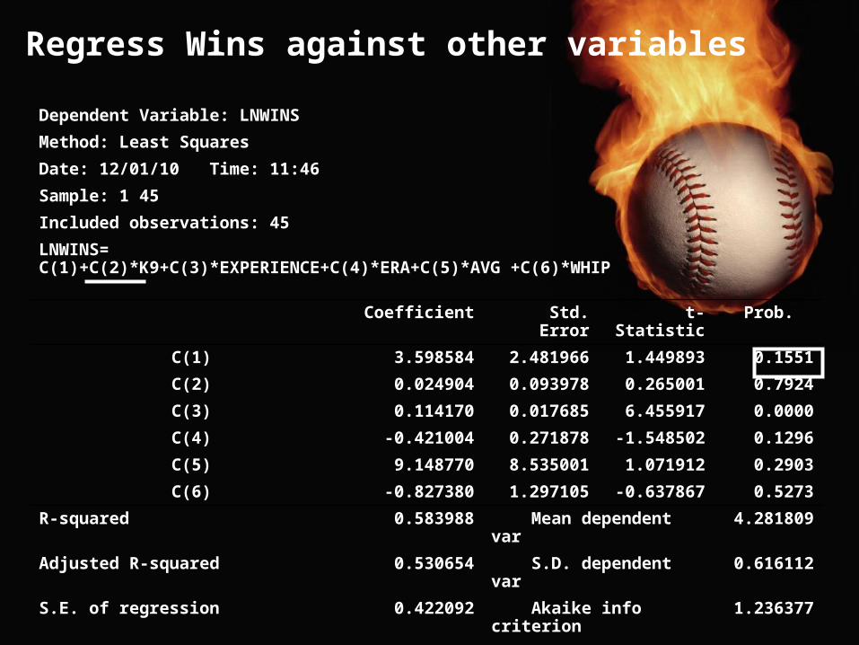
Regress Wins against other variables
Dependent Variable: LNWINS
Method: Least Squares
Date: 12/01/10 Time: 11:46
Sample: 1 45
Included observations: 45
LNWINS=C(1)+C(2)*K9+C(3)*EXPERIENCE+C(4)*ERA+C(5)*AVG +C(6)*WHIP
Coefficient Std. Error t-Statistic Prob.
C(1) 3.598584 2.481966 1.449893 0.1551
C(2) 0.024904 0.093978 0.265001 0.7924
C(3) 0.114170 0.017685 6.455917 0.0000
C(4) -0.421004 0.271878 -1.548502 0.1296
C(5) 9.148770 8.535001 1.071912 0.2903
C(6) -0.827380 1.297105 -0.637867 0.5273
R-squared 0.583988 Mean dependent var 4.281809
Adjusted R-squared 0.530654 S.D. dependent var 0.616112
S.E. of regression 0.422092 Akaike info criterion 1.236377
Sum squared resid 6.948293 Schwarz criterion 1.477265
Log likelihood -21.81849 F-statistic 10.94948
Durbin-Watson stat 1.656059 Prob(F-statistic) 0.000001
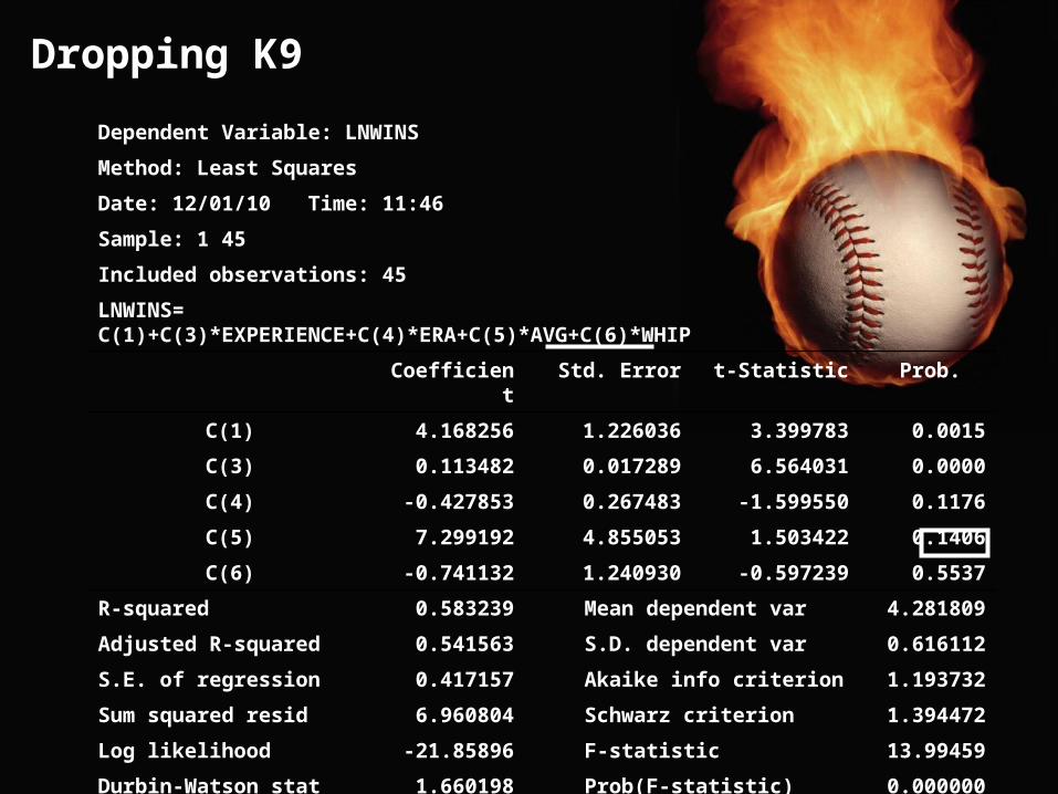
Dropping K9
Dependent Variable: LNWINS
Method: Least Squares
Date: 12/01/10 Time: 11:46
Sample: 1 45
Included observations: 45
LNWINS=C(1)+C(3)*EXPERIENCE+C(4)*ERA+C(5)*AVG+C(6)*WHIP
Coefficient Std. Error t-Statistic Prob.
C(1) 4.168256 1.226036 3.399783 0.0015
C(3) 0.113482 0.017289 6.564031 0.0000
C(4) -0.427853 0.267483 -1.599550 0.1176
C(5) 7.299192 4.855053 1.503422 0.1406
C(6) -0.741132 1.240930 -0.597239 0.5537
R-squared 0.583239 Mean dependent var 4.281809
Adjusted R-squared 0.541563 S.D. dependent var 0.616112
S.E. of regression 0.417157 Akaike info criterion 1.193732
Sum squared resid 6.960804 Schwarz criterion 1.394472
Log likelihood -21.85896 F-statistic 13.99459
Durbin-Watson stat 1.660198 Prob(F-statistic) 0.000000
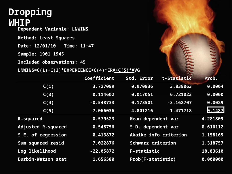
Dropping WHIP
Dependent Variable: LNWINS
Method: Least Squares
Date: 12/01/10 Time: 11:47
Sample: 1901 1945
Included observations: 45
LNWINS=C(1)+C(3)*EXPERIENCE+C(4)*ERA+C(5)*AVG
Coefficient Std. Error t-Statistic Prob.
C(1) 3.727099 0.970836 3.839063 0.0004
C(3) 0.114602 0.017051 6.721023 0.0000
C(4) -0.548733 0.173501 -3.162707 0.0029
C(5) 7.066036 4.801216 1.471718 0.1487
R-squared 0.579523 Mean dependent var 4.281809
Adjusted R-squared 0.548756 S.D. dependent var 0.616112
S.E. of regression 0.413872 Akaike info criterion 1.158165
Sum squared resid 7.022876 Schwarz criterion 1.318757
Log likelihood -22.05872 F-statistic 18.83610
Durbin-Watson stat 1.656580 Prob(F-statistic) 0.000000
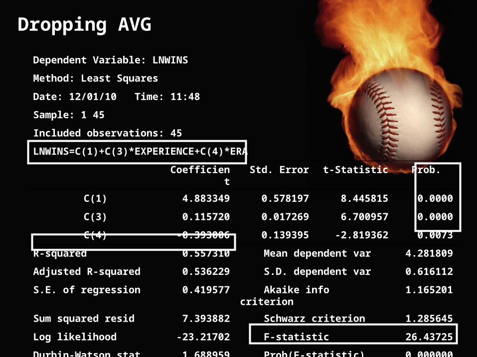
Dropping AVG
Dependent Variable: LNWINS
Method: Least Squares
Date: 12/01/10 Time: 11:48
Sample: 1 45
Included observations: 45
LNWINS=C(1)+C(3)*EXPERIENCE+C(4)*ERA
Coefficient Std. Error t-Statistic Prob.
C(1) 4.883349 0.578197 8.445815 0.0000
C(3) 0.115720 0.017269 6.700957 0.0000
C(4) -0.393006 0.139395 -2.819362 0.0073
R-squared 0.557310 Mean dependent var 4.281809
Adjusted R-squared 0.536229 S.D. dependent var 0.616112
S.E. of regression 0.419577 Akaike info criterion 1.165201
Sum squared resid 7.393882 Schwarz criterion 1.285645
Log likelihood -23.21702 F-statistic 26.43725
Durbin-Watson stat 1.688959 Prob(F-statistic) 0.000000
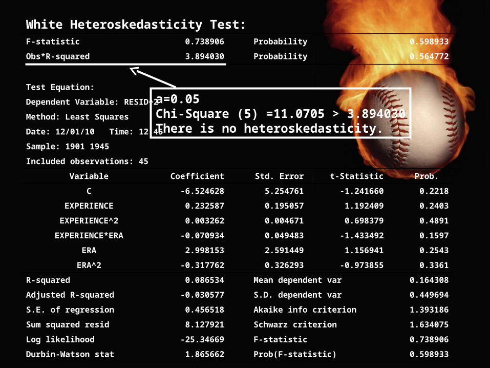
White Heteroskedasticity Test:F-statistic 0.738906 Probability 0.598933
Obs*R-squared 3.894030 Probability 0.564772
Test Equation:
Dependent Variable: RESID^2
Method: Least Squares
Date: 12/01/10 Time: 12:45
Sample: 1901 1945
Included observations: 45
Variable Coefficient Std. Error t-Statistic Prob.
C -6.524628 5.254761 -1.241660 0.2218
EXPERIENCE 0.232587 0.195057 1.192409 0.2403
EXPERIENCE^2 0.003262 0.004671 0.698379 0.4891
EXPERIENCE*ERA -0.070934 0.049483 -1.433492 0.1597
ERA 2.998153 2.591449 1.156941 0.2543
ERA^2 -0.317762 0.326293 -0.973855 0.3361
R-squared 0.086534 Mean dependent var 0.164308
Adjusted R-squared -0.030577 S.D. dependent var 0.449694
S.E. of regression 0.456518 Akaike info criterion 1.393186
Sum squared resid 8.127921 Schwarz criterion 1.634075
Log likelihood -25.34669 F-statistic 0.738906
Durbin-Watson stat 1.865662 Prob(F-statistic) 0.598933
a=0.05Chi-Square (5) =11.0705 > 3.894030There is no heteroskedasticity.

We get that experience and ERA are the most important factors in determining how many wins a player has. It is intuitive that the longer the player is in the league, the more wins he will inevitably receive, but it also is important to note that ERA is the most important performance statistic in determining the number of wins.
Conclusion 1

Regress Salary against other variables
Dependent Variable: SALARY
Method: Least Squares
Date: 11/29/10 Time: 22:16
Sample: 1 45
Included observations: 45
SALARY=C(1)+C(2)*K9+C(3)*ERA+C(4)*EXPERIENCE+C(5)*AVG
+C(6)*WINS+C(7)*WHIP
Coefficient Std. Error t-Statistic Prob.
C(1) 13.26240 26.93882 0.492315 0.6253
C(2) 0.535060 1.019848 0.524647 0.6029
C(3) -5.824067 3.073178 -1.895128 0.0657
C(4) 0.965893 0.298615 3.234570 0.0025
C(5) 39.57241 94.30549 0.419619 0.6771
C(6) 0.010538 0.022938 0.459394 0.6486
C(7) -3.340880 14.13198 -0.236406 0.8144
R-squared 0.571672 Mean dependent var 8.531823
Adjusted R-squared 0.504041 S.D. dependent var 6.503770
S.E. of regression 4.580238 Akaike info criterion 6.023414
Sum squared resid 797.1862 Schwarz criterion 6.304450
Log likelihood -128.5268 F-statistic 8.452832
Durbin-Watson stat 1.995391 Prob(F-statistic) 0.000007

Dropping WHIP
Dependent Variable: SALARY
Method: Least Squares
Date: 11/29/10 Time: 22:17
Sample: 1 45
Included observations: 45
SALARY=C(1)+C(2)*K9+C(3)*ERA+C(4)*EXPERIENCE+C(5)*AVG
+C(6)*WINS
Coefficient Std. Error t-Statistic Prob.
C(1) 12.77971 26.53421 0.481631 0.6328
C(2) 0.474565 0.975198 0.486634 0.6292
C(3) -6.328931 2.182998 -2.899193 0.0061
C(4) 0.964078 0.294881 3.269375 0.0023
C(5) 33.74487 89.91824 0.375284 0.7095
C(6) 0.011023 0.022568 0.488440 0.6280
R-squared 0.571042 Mean dependent var 8.531823
Adjusted R-squared 0.516047 S.D. dependent var 6.503770
S.E. of regression 4.524459 Akaike info criterion 5.980439
Sum squared resid 798.3586 Schwarz criterion 6.221327
Log likelihood -128.5599 F-statistic 10.38359
Durbin-Watson stat 1.985975 Prob(F-statistic) 0.000002
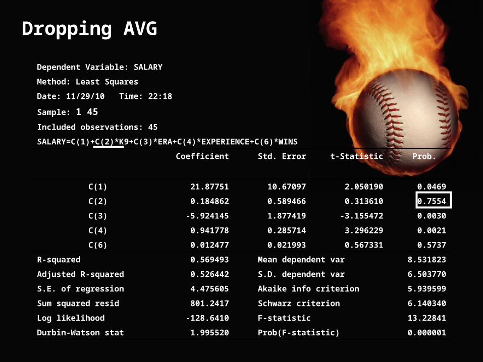
Dropping AVG
Dependent Variable: SALARY
Method: Least Squares
Date: 11/29/10 Time: 22:18
Sample: 1 45
Included observations: 45
SALARY=C(1)+C(2)*K9+C(3)*ERA+C(4)*EXPERIENCE+C(6)*WINS
Coefficient Std. Error t-Statistic Prob.
C(1) 21.87751 10.67097 2.050190 0.0469
C(2) 0.184862 0.589466 0.313610 0.7554
C(3) -5.924145 1.877419 -3.155472 0.0030
C(4) 0.941778 0.285714 3.296229 0.0021
C(6) 0.012477 0.021993 0.567331 0.5737
R-squared 0.569493 Mean dependent var 8.531823
Adjusted R-squared 0.526442 S.D. dependent var 6.503770
S.E. of regression 4.475605 Akaike info criterion 5.939599
Sum squared resid 801.2417 Schwarz criterion 6.140340
Log likelihood -128.6410 F-statistic 13.22841
Durbin-Watson stat 1.995520 Prob(F-statistic) 0.000001
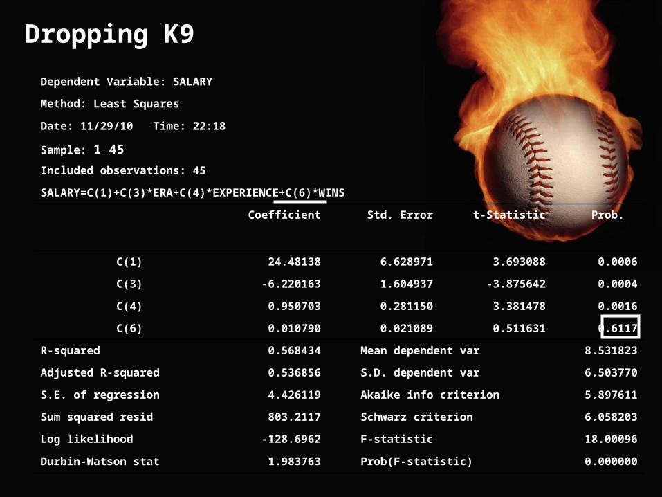
Dropping K9
Dependent Variable: SALARY
Method: Least Squares
Date: 11/29/10 Time: 22:18
Sample: 1 45
Included observations: 45
SALARY=C(1)+C(3)*ERA+C(4)*EXPERIENCE+C(6)*WINS
Coefficient Std. Error t-Statistic Prob.
C(1) 24.48138 6.628971 3.693088 0.0006
C(3) -6.220163 1.604937 -3.875642 0.0004
C(4) 0.950703 0.281150 3.381478 0.0016
C(6) 0.010790 0.021089 0.511631 0.6117
R-squared 0.568434 Mean dependent var 8.531823
Adjusted R-squared 0.536856 S.D. dependent var 6.503770
S.E. of regression 4.426119 Akaike info criterion 5.897611
Sum squared resid 803.2117 Schwarz criterion 6.058203
Log likelihood -128.6962 F-statistic 18.00096
Durbin-Watson stat 1.983763 Prob(F-statistic) 0.000000

Dropping WINS
Dependent Variable: SALARY
Method: Least Squares
Date: 11/29/10 Time: 21:48
Sample: 1 45
Included observations: 45
SALARY=C(1)+C(3)*ERA+C(4)*EXPERIENCE
Coefficient Std. Error t-Statistic Prob.
C(1) 25.80969 6.045566 4.269194 0.0001
C(3) -6.549164 1.457502 -4.493416 0.0001
C(4) 1.060266 0.180564 5.871959 0.0000
R-squared 0.565679 Mean dependent var 8.531823
Adjusted R-squared 0.544997 S.D. dependent var 6.503770
S.E. of regression 4.387048 Akaike info criterion 5.859530
Sum squared resid 808.3399 Schwarz criterion 5.979975
Log likelihood -128.8394 F-statistic 27.35131
Durbin-Watson stat 1.967714 Prob(F-statistic) 0.000000

White Heteroskedasticity Test:
F-statistic 3.148422 Probability 0.017555
Obs*R-squared 12.94058 Probability 0.023942
Test Equation:
Dependent Variable: RESID^2
Method: Least Squares
Date: 11/30/10 Time: 16:14
Sample: 1901 1945
Included observations: 45
Variable Coefficient Std. Error t-Statistic Prob.
C 250.6808 336.6494 0.744634 0.4610
ERA -81.81855 166.0227 -0.492815 0.6249
ERA^2 6.237881 20.90415 0.298404 0.7670
ERA*EXPERIENCE 4.320411 3.170161 1.362836 0.1808
EXPERIENCE -23.21171 12.49642 -1.857468 0.0708
EXPERIENCE^2 0.519519 0.299279 1.735900 0.0905
R-squared 0.287569 Mean dependent var 17.96311
Adjusted R-squared 0.196231 S.D. dependent var 32.62247
S.E. of regression 29.24707 Akaike info criterion 9.713002
Sum squared resid 33360.26 Schwarz criterion 9.953890
Log likelihood -212.5425 F-statistic 3.148422
Durbin-Watson stat 1.975917 Prob(F-statistic) 0.017555
a=0.05Chi-Square (5) = 11.0705<12.94058So there is Heteroskedasticity.

We come to the same conclusion for salary. Experience and ERA are the main contributing factors to salary as we found before for wins.
Conclusion 2
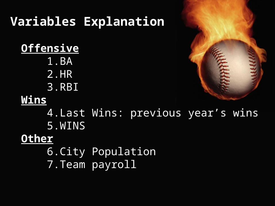
Offensive 1.BA 2.HR 3.RBIWins 4.Last Wins: previous year’s wins 5.WINSOther 6.City Population 7.Team payroll
Variables Explanation
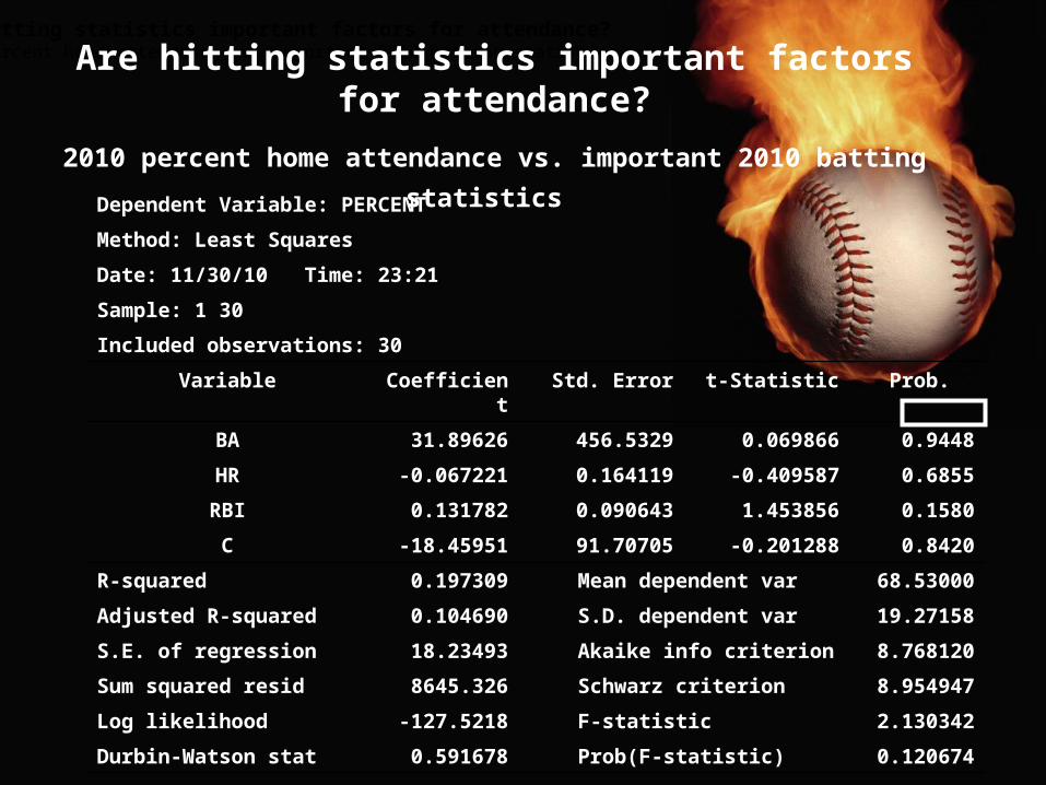
Are hitting statistics important factors for attendance? 2010 percent home attendance vs. important 2010 batting statistics
Dependent Variable: PERCENT
Method: Least Squares
Date: 11/30/10 Time: 23:21
Sample: 1 30
Included observations: 30
Variable Coefficient Std. Error t-Statistic Prob.
BA 31.89626 456.5329 0.069866 0.9448
HR -0.067221 0.164119 -0.409587 0.6855
RBI 0.131782 0.090643 1.453856 0.1580
C -18.45951 91.70705 -0.201288 0.8420
R-squared 0.197309 Mean dependent var 68.53000
Adjusted R-squared 0.104690 S.D. dependent var 19.27158
S.E. of regression 18.23493 Akaike info criterion 8.768120
Sum squared resid 8645.326 Schwarz criterion 8.954947
Log likelihood -127.5218 F-statistic 2.130342
Durbin-Watson stat 0.591678 Prob(F-statistic) 0.120674
Are hitting statistics important factors for attendance?
2010 percent home attendance vs. important 2010 batting statistics
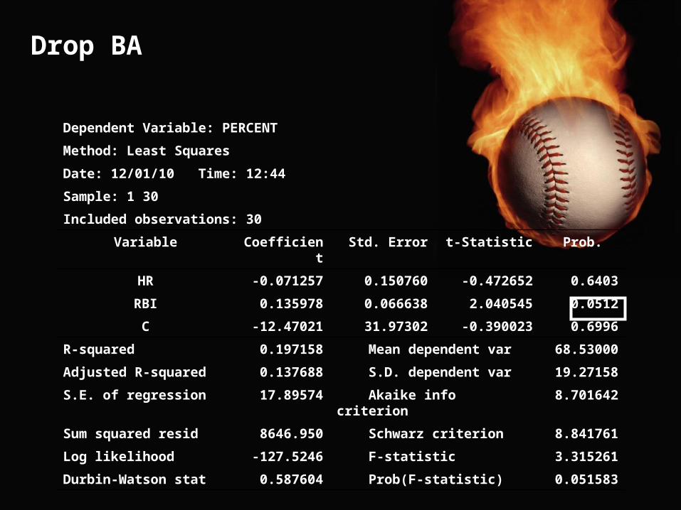
Dependent Variable: PERCENT
Method: Least Squares
Date: 12/01/10 Time: 12:44
Sample: 1 30
Included observations: 30
Variable Coefficient Std. Error t-Statistic Prob.
HR -0.071257 0.150760 -0.472652 0.6403
RBI 0.135978 0.066638 2.040545 0.0512
C -12.47021 31.97302 -0.390023 0.6996
R-squared 0.197158 Mean dependent var 68.53000
Adjusted R-squared 0.137688 S.D. dependent var 19.27158
S.E. of regression 17.89574 Akaike info criterion 8.701642
Sum squared resid 8646.950 Schwarz criterion 8.841761
Log likelihood -127.5246 F-statistic 3.315261
Durbin-Watson stat 0.587604 Prob(F-statistic) 0.051583
Drop BA

Drop Constant
Dependent Variable: PERCENT
Method: Least Squares
Date: 12/01/10 Time: 12:40
Sample: 1 30
Included observations: 30
Variable Coefficient Std. Error t-Statistic Prob.
RBI 0.113385 0.032437 3.495558 0.0016
HR -0.052144 0.140397 -0.371400 0.7131
R-squared 0.192635 Mean dependent var 68.53000
Adjusted R-squared 0.163800 S.D. dependent var 19.27158
S.E. of regression 17.62270 Akaike info criterion 8.640593
Sum squared resid 8695.666 Schwarz criterion 8.734006
Log likelihood -127.6089 F-statistic 6.680705
Durbin-Watson stat 0.481354 Prob(F-statistic) 0.015250
RBI’S ARE THE MOST IMPORTANT OFFENSIVE STATISTIC
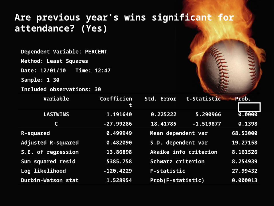
Are previous year’s wins significant for attendance? (Yes)
Dependent Variable: PERCENT
Method: Least Squares
Date: 12/01/10 Time: 12:47
Sample: 1 30
Included observations: 30
Variable Coefficient Std. Error t-Statistic Prob.
LASTWINS 1.191640 0.225222 5.290966 0.0000
C -27.99286 18.41785 -1.519877 0.1398
R-squared 0.499949 Mean dependent var 68.53000
Adjusted R-squared 0.482090 S.D. dependent var 19.27158
S.E. of regression 13.86898 Akaike info criterion 8.161526
Sum squared resid 5385.758 Schwarz criterion 8.254939
Log likelihood -120.4229 F-statistic 27.99432
Durbin-Watson stat 1.528954 Prob(F-statistic) 0.000013
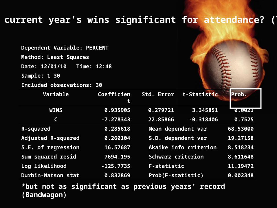
Are current year’s wins significant for attendance? (Yes)*
Dependent Variable: PERCENT
Method: Least Squares
Date: 12/01/10 Time: 12:48
Sample: 1 30
Included observations: 30
Variable Coefficient Std. Error t-Statistic Prob.
WINS 0.935905 0.279721 3.345851 0.0023
C -7.278343 22.85866 -0.318406 0.7525
R-squared 0.285618 Mean dependent var 68.53000
Adjusted R-squared 0.260104 S.D. dependent var 19.27158
S.E. of regression 16.57687 Akaike info criterion 8.518234
Sum squared resid 7694.195 Schwarz criterion 8.611648
Log likelihood -125.7735 F-statistic 11.19472
Durbin-Watson stat 0.832869 Prob(F-statistic) 0.002348
*but not as significant as previous years’ record (Bandwagon)

Is city population significant for attendance? (No)
Dependent Variable: PERCENT
Method: Least Squares
Date: 12/01/10 Time: 12:51
Sample: 1 30
Included observations: 30
Variable Coefficient Std. Error t-Statistic Prob.
CITYPOP 2.95E-06 1.64E-06 1.797594 0.0830
C 63.59600 4.362240 14.57875 0.0000
R-squared 0.103465 Mean dependent var 68.53000
Adjusted R-squared 0.071446 S.D. dependent var 19.27158
S.E. of regression 18.57039 Akaike info criterion 8.745354
Sum squared resid 9656.063 Schwarz criterion 8.838767
Log likelihood -129.1803 F-statistic 3.231345
Durbin-Watson stat 0.609337 Prob(F-statistic) 0.083035
-It’s more general baseball enthusiasm rather than population:E.g. Boston population= 645,169 Attendance%=100.9% Arizona population= 1,601,587 Attendance%=51.8%
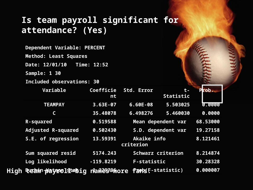
Is team payroll significant for attendance? (Yes)
Dependent Variable: PERCENT
Method: Least Squares
Date: 12/01/10 Time: 12:52
Sample: 1 30
Included observations: 30
Variable Coefficient Std. Error t-Statistic Prob.
TEAMPAY 3.63E-07 6.60E-08 5.503025 0.0000
C 35.48078 6.498276 5.460030 0.0000
R-squared 0.519588 Mean dependent var 68.53000
Adjusted R-squared 0.502430 S.D. dependent var 19.27158
S.E. of regression 13.59391 Akaike info criterion 8.121461
Sum squared resid 5174.243 Schwarz criterion 8.214874
Log likelihood -119.8219 F-statistic 30.28328
Durbin-Watson stat 1.229796 Prob(F-statistic) 0.000007
High team payroll=big names=more fans.

Are city population and payroll correlated?
Dependent Variable: CITYPOP
Method: Least Squares
Date: 11/30/10 Time: 23:57
Sample: 1 30
Included observations: 30
Variable Coefficient Std. Error t-Statistic Prob.
TEAMPAY 0.033187 0.008261 4.017155 0.0004
C -1349341. 813618.3 -1.658444 0.1084
R-squared 0.365619 Mean dependent var 1671312.
Adjusted R-squared 0.342963 S.D. dependent var 2099771.
S.E. of regression 1702029. Akaike info criterion 31.59688
Sum squared resid 8.11E+13 Schwarz criterion 31.69029
Log likelihood -471.9532 F-statistic 16.13753
Durbin-Watson stat 2.409794 Prob(F-statistic) 0.000401
Even though big cities don’t necessarily lead to high att.%, it is correlated with team payroll. There is an indirect affect from city pop, larger pop=>higher payroll=>attracts big names.
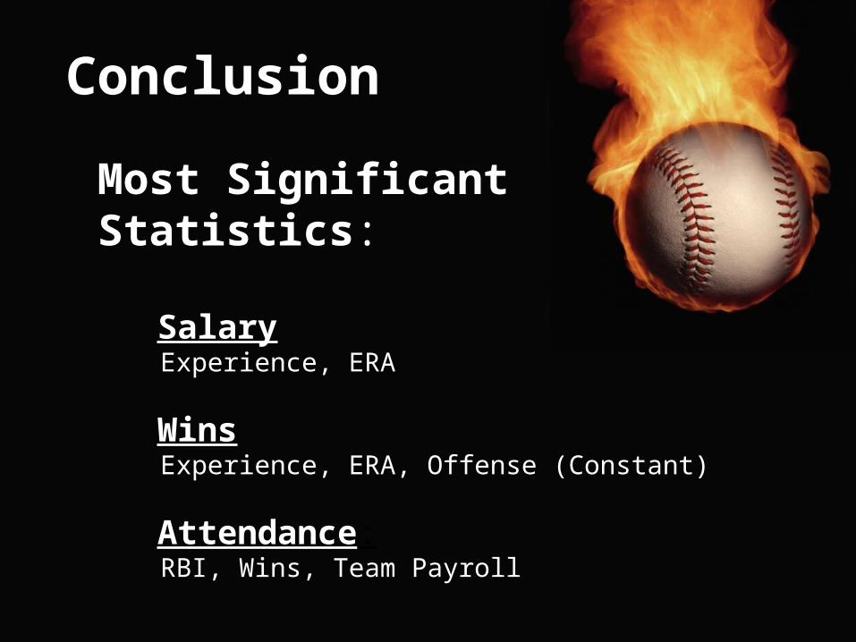
Conclusion
Most Significant Statistics:
Salary Experience, ERA
Wins Experience, ERA, Offense (Constant)
Attendance: RBI, Wins, Team Payroll

Questions?