Embed Size (px)
Citation preview
MLJVM: A Java Virtual Machine implemented
in Standard ML
Laura Korte - [email protected]
Supervised by Stephen Gilmore
MSc Computer Science
University of Edinburgh
2003
Abstract
This thesis describes the MLJVM, a Java Virtual Machine written in the impure functional language
Standard ML. Being the first of its kind in this functional approach, my thesis provides not only a
detailed description of the implementation of the MLJVM, but also some insight into the pros and
cons of a functional JVM.
Contents
1 Introduction 5
1.1 Motivation . . . . . . . . . . . . . . . . . . . . . . . . . . . . . . . . . . . . . . . . . 6
1.2 Java Virtual Machine . . . . . . . . . . . . . . . . . . . . . . . . . . . . . . . . . . . 6
1.3 Standard ML . . . . . . . . . . . . . . . . . . . . . . . . . . . . . . . . . . . . . . . . 7
1.4 SML-JVM Toolkit . . . . . . . . . . . . . . . . . . . . . . . . . . . . . . . . . . . . . 8
1.5 Grail . . . . . . . . . . . . . . . . . . . . . . . . . . . . . . . . . . . . . . . . . . . . . 9
1.6 Jasmin . . . . . . . . . . . . . . . . . . . . . . . . . . . . . . . . . . . . . . . . . . . . 9
2 Design 11
2.1 Overview . . . . . . . . . . . . . . . . . . . . . . . . . . . . . . . . . . . . . . . . . . 11
2.2 Parser . . . . . . . . . . . . . . . . . . . . . . . . . . . . . . . . . . . . . . . . . . . . 11
2.3 The Datatype Conversion Problem . . . . . . . . . . . . . . . . . . . . . . . . . . . . 11
2.4 Initial Environment . . . . . . . . . . . . . . . . . . . . . . . . . . . . . . . . . . . . . 13
2.5 Executing a Classfile . . . . . . . . . . . . . . . . . . . . . . . . . . . . . . . . . . . . 13
2.6 Printing a Classfile . . . . . . . . . . . . . . . . . . . . . . . . . . . . . . . . . . . . . 14
3 Implementation 15
3.1 Parser.sml . . . . . . . . . . . . . . . . . . . . . . . . . . . . . . . . . . . . . . . . . . 15
3.2 Bytecode2.sml . . . . . . . . . . . . . . . . . . . . . . . . . . . . . . . . . . . . . . . 16
3.3 Int32.sml . . . . . . . . . . . . . . . . . . . . . . . . . . . . . . . . . . . . . . . . . . 16
3.4 MyClassFile.sml . . . . . . . . . . . . . . . . . . . . . . . . . . . . . . . . . . . . . . 18
3.5 Transform.sml . . . . . . . . . . . . . . . . . . . . . . . . . . . . . . . . . . . . . . . . 18
3.6 RuntimeClass.sml & RuntimePool.sml . . . . . . . . . . . . . . . . . . . . . . . . . . 19
3.7 Error.sml . . . . . . . . . . . . . . . . . . . . . . . . . . . . . . . . . . . . . . . . . . 23
3.8 Modifiers.sml . . . . . . . . . . . . . . . . . . . . . . . . . . . . . . . . . . . . . . . . 23
3.9 JasminPrint.sml . . . . . . . . . . . . . . . . . . . . . . . . . . . . . . . . . . . . . . 23
3.10 Heap.sml . . . . . . . . . . . . . . . . . . . . . . . . . . . . . . . . . . . . . . . . . . 24
3.11 Environment.sml . . . . . . . . . . . . . . . . . . . . . . . . . . . . . . . . . . . . . . 26
3.12 Execute.sml . . . . . . . . . . . . . . . . . . . . . . . . . . . . . . . . . . . . . . . . . 26
4 Running the MLJVM on some examples 32
4.1 Example 1 – Parsing a Method Type . . . . . . . . . . . . . . . . . . . . . . . . . . . 32
4.2 Example 2 – Lookup Hash and Data Array . . . . . . . . . . . . . . . . . . . . . . . 32
4.3 Example 3 – Pre-Defined Attribute Array . . . . . . . . . . . . . . . . . . . . . . . . 33
4.4 Example 4 – Execution of Some Simple Methods . . . . . . . . . . . . . . . . . . . . 33
4.5 Example 5 – Parse Offset . . . . . . . . . . . . . . . . . . . . . . . . . . . . . . . . . 34
1

4.6 Example 6 – Jasmin Pretty Printer . . . . . . . . . . . . . . . . . . . . . . . . . . . . 35
4.7 Example 7 – About Superclasses . . . . . . . . . . . . . . . . . . . . . . . . . . . . . 37
4.8 Example 8 – Execution Speed . . . . . . . . . . . . . . . . . . . . . . . . . . . . . . . 38
4.9 Example 9 – Generating Exceptions . . . . . . . . . . . . . . . . . . . . . . . . . . . 40
4.10 Example 10 – Debugging the MLJVM . . . . . . . . . . . . . . . . . . . . . . . . . . 41
5 Conclusions 44
5.1 Discussion . . . . . . . . . . . . . . . . . . . . . . . . . . . . . . . . . . . . . . . . . . 44
5.2 Future Work . . . . . . . . . . . . . . . . . . . . . . . . . . . . . . . . . . . . . . . . 45
5.3 Conclusion . . . . . . . . . . . . . . . . . . . . . . . . . . . . . . . . . . . . . . . . . 47
A MLJVM Mini Manual 50
B Grail Examples 51
B.1 HelloWorld.gr . . . . . . . . . . . . . . . . . . . . . . . . . . . . . . . . . . . . . . . . 51
B.2 Fib.gr . . . . . . . . . . . . . . . . . . . . . . . . . . . . . . . . . . . . . . . . . . . . 52
B.3 SumList.gr . . . . . . . . . . . . . . . . . . . . . . . . . . . . . . . . . . . . . . . . . 54
C Java Examples 55
C.1 Q1.java, Q2.java and Q3.java . . . . . . . . . . . . . . . . . . . . . . . . . . . . . . . 55
C.2 ExOne.java . . . . . . . . . . . . . . . . . . . . . . . . . . . . . . . . . . . . . . . . . 56
C.3 ExTwo.java . . . . . . . . . . . . . . . . . . . . . . . . . . . . . . . . . . . . . . . . . 57
C.4 ExThree.java . . . . . . . . . . . . . . . . . . . . . . . . . . . . . . . . . . . . . . . . 58
2

Acknowledgements
First of all I would like to thank my supervisor Stephen Gilmore who was always optimistic even
when I was not, and taught me not to use exclamation marks in my dissertation! I would also
like to thank David Aspinall for being my substitute supervisor and second marker, the Dutch
Government and the VSB Fund for making it financially possible for me to come to Edinburgh,
my friends from all over the world for making my MSc year in Edinburgh into a year I will never
forget, and last but certainly not least, I would like to thank my parents for their love and support.
You are the reason I made it to Edinburgh in the first place. Many thanks for being there.
3

Declaration
I declare that this thesis was composed by myself, that the work contained herein is my own except
where explicitly stated otherwise in the text, and that this work has not been submitted for any
other degree or professional qualification except as specified.
Laura Korte.
4
1 Introduction
Some eight years after Java was first announced to the world on May 23rd 1995, the majority of the
major technology companies has now produced at least one Java Virtual Machine (JVM). Often
presented as part of a Java Development Kit (JDK) or Java Runtime Environment (JRE), Java
Virtual Machines have been implemented by (among others) Apple, FreeBSD, Fujitsu-Siemens,
Hewlett-Packard, IBM, Microsoft, Novell, OpenBSD, Oracle, Psion and of course Sun. This thesis
is concerned with the implementation of a new sort of Java Virtual Machine: the functional JVM
as part of a limited JRE.
Inevitably the following question springs to mind: “In this jungle of JVMs, JREs and JDKs
produced by software giants, why bring yet another one into existence?” The answer lies not so
much in the performance or capabilities of the JVM, but in the language it has been implemented
in: it so happens that most of the JVMs have been implemented in C, C++ or even Java itself,
but none have been implemented in a functional language.
Of course there are many additional questions: Would a functional JVM have any advantages
over one programmed in a language like C, C++ or Java? Would there be disadvantages? What
about those typically object oriented features of Java, like the creation and manipulation of ob-
jects? Would they prove to be a problem for a functional JVM? How will the native classes be
implemented? This thesis aims to provide an answer to questions like that by presenting a Java
Virtual Machine implemented in the functional language Standard ML.
While the MLJVM is indeed the first JVM to be implemented in a functional language, it is
certainly not the first attempt to merge Java and Standard ML. The SML-JVM Toolkit for example,
of which several parts will be used by the MLJVM, provides an alternative back-end for the Moscow
ML compiler, which causes it to output Java bytecode rather than the usual Caml-like bytecode.
The SML-JVM Toolkit is described in [Ber98]. Another example of merging Java and Standard ML
is MLj, as described in [Ben98], [Ben99] and [MLj99]. MLj is a stand-alone compiler for Standard
ML which targets Java bytecode. It also allows the ML programmer to access the extensive Java
libraries and other Java programs. Finally, a compiler for both Java and ML has been proposed in
the recent FLINT paper [Lea03]. This compiler targets a new intermediate language and will allow
both Java and ML programs to be executed in the same runtime environment.
The outline of the rest of this thesis will be as follows: after presenting my motivation for writing
this thesis and a brief introduction to some of its most important concepts, Standard ML, the Java
Virtual Machine (JVM), Jasmin and Grail, I will describe the MLJVM in increasing detail. This
means I will start by giving the abstract design (Section 2), then go on to the implementation
(Section 3) and conclude by giving numerous examples (Section 4) to illustrate the working of
the MLJVM. Finally, a discussion of the MLJVM, future work and the conclusions will be presented
in Section 5.
5
1.1 Motivation
As mentioned in the introduction, one of the reasons for designing the MLJVM described in this
thesis, was the fact that the MLJVM was going to be the first of its kind: the first JVM to be
implemented in a functional language. Moreover, this functional JVM would – just like all other
programs written in ML – be type-safe and have a wider range of implementation techniques avail-
able (e.g. higher-order functions) than is available when implementing in a traditional imperative
language. This implementation platform is in contrast to JVMs written in languages like C or C++,
which can neither guarantee any form of type-safety, nor have the opportunity to use high-order
functions. Java does guarantee some type-safety, but Java’s type-safety is inferior compared to
ML’s and like C and C++, Java has no support for higher-order functions. Furthermore, Standard
ML also provides – like most other functional languages – a very concise way of programming.
Compared to a JVM in C, C++ or Java, our JVM will inevitably be shorter.
There are of course other functional languages available, but our choice fell on ML for multiple
reasons. First of all, Standard ML is an impure functional programming language with some
imperative features which would prove extremely useful in implementing the MLJVM. Furthermore,
ML’s design of structures and signatures makes large programs easier to structure and develop and
finally, the SML-JVM Toolkit (Section 1.4) of which we recycled a substantial amount was written
in ML. This recycling would not have been possible should we have decided to implement our
functional JVM in a different (functional) language.
As for the subset of JVM instructions that was to be implemented, we used jGrail. This subset
provided only the basic functionality of Java bytecode, but was at the same time much more than
just a toy language. It has very real applications in the ongoing research program Mobile Resource
Guarantees at the Edinburgh University.
The only drawback using jGrail as our subset had, was the fact that Grail is – just like ML
– functional. This means that a MLJVM implementing just the jGrail instruction set would only
demonstrate how to execute functional programs which have been compiled to Java bytecode. Much
more interesting would be if could execute instructions that are clearly imperative or even better,
object-oriented.
For that purpose the MLJVM does not only support the entire jGrail instruction set, but also
instructions for updating static fields, the creation and manipulation of objects and arrays, and the
possibility to define your own class hierarchy by extending classes.
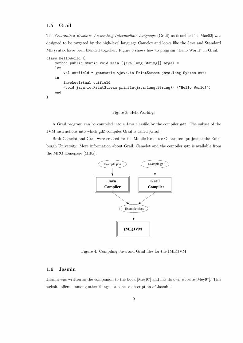
1.2 Java Virtual Machine
The Java Virtual Machine, or JVM for short, is a program for executing Java classfiles. So in order
to execute a Java program, one will first need a Java compiler to compile it into one or more Java
classfiles. The product of this compilation (the Java classfiles) can then be executed on a JVM
6

(Figure 4).
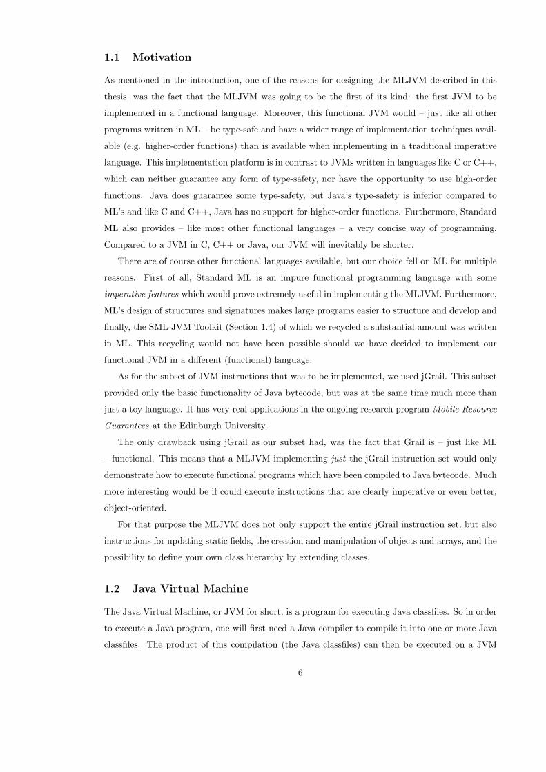
Two important concepts of the JVM are frames and stacks. Each session of a single threaded
JVM has exactly one stack. This stack is a FILO queue (first-in-last-out) onto which the so-called
frames can be pushed. In turn, each individual frame has its own stack, which are also FILO queues
but instead of frames, values like integers or object pointers will be pushed onto and popped off
these ones.
A frame represents a method being executed and therefore also has to keep track of an array of
JVM instructions. With this array comes a counter which holds the index of the instruction that
the MLJVM is currently executing. Once a method finishes, the frame representing that method
is popped off the stack and control is handed back to the invoking method. If the method has a
void return type, that is all that happens but if the method has a return value, this value will be
pushed onto the stack of the invoking frame before popping the finished frame off the JVM stack.
Heap
object
frame
frame
frame
frame
object
object
object
object
objectclass
class
class
JVM Environment
Method Area Stack
Figure 1: The Java Virtual Machine Environment
Apart from the stack with all the frames on it, there are several other things the JVM has to
store. The two most important are the method area and the heap. The method area, heap and
stack are all stored in the JVM’s environment. The method area is where all loaded classes with
their fields and methods are, and the heap is where one would find all created objects (Figure 1).
Both of these areas and the JVM stack are shared, which means all methods have access to the
same JVM stack, method area and heap. In contrast, the stacks inside the frames are private. No
method has access to another method’s stack, only to its own.
1.3 Standard ML
Standard ML is an eager, impure, functional programming language. Eager, because it uses a call-
by-value normalisation strategy rather than a lazy one like call-by-need or call-by-value. Impure,
because it also has imperative features like pointers and assignments. And functional because
7
like all other functional programming languages its design was based on the λ-calculus, in which
normalisation takes the role of execution. Functional languages also have the property of being
concise. It typically takes a programmer fewer lines to write a program in a functional language,
than it would take him to write it in an imperative one.
Furthermore, Standard ML uses functors, structures and signatures which are helpful when
designing a large piece of software, and like many other functional programming languages, the
unique control-flow mechanism of call/cc and continuations is present in Standard ML. More
information about Standard ML can be found in [Pau96].
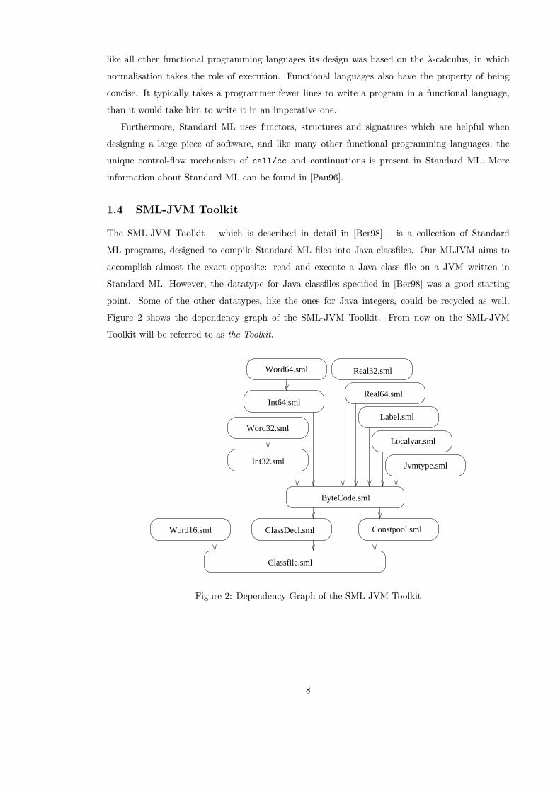
1.4 SML-JVM Toolkit
The SML-JVM Toolkit – which is described in detail in [Ber98] – is a collection of Standard
ML programs, designed to compile Standard ML files into Java classfiles. Our MLJVM aims to
accomplish almost the exact opposite: read and execute a Java class file on a JVM written in
Standard ML. However, the datatype for Java classfiles specified in [Ber98] was a good starting
point. Some of the other datatypes, like the ones for Java integers, could be recycled as well.
Figure 2 shows the dependency graph of the SML-JVM Toolkit. From now on the SML-JVM
Toolkit will be referred to as the Toolkit.
ByteCode.sml
Localvar.sml
Int64.sml
Word64.sml
Int32.sml
Word32.sml
Word16.sml Constpool.sml
Label.sml
Jvmtype.sml
ClassDecl.sml
Real64.sml
Real32.sml
Classfile.sml
Figure 2: Dependency Graph of the SML-JVM Toolkit
8
1.5 Grail
The Guaranteed Resource Accounting Intermediate Language (Grail) as described in [Mac02] was
designed to be targeted by the high-level language Camelot and looks like the Java and Standard
ML syntax have been blended together. Figure 3 shows how to program ”Hello World” in Grail.
class HelloWorld {
method public static void main (java.lang.String[] args) =
let
val outfield = getstatic <java.io.PrintStream java.lang.System.out>
in
invokevirtual outfield
<void java.io.PrintStream.println(java.lang.String)> ("Hello World!")
end
}
Figure 3: HelloWorld.gr
A Grail program can be compiled into a Java classfile by the compiler gdf. The subset of the
JVM instructions into which gdf compiles Grail is called jGrail.
Both Camelot and Grail were created for the Mobile Resource Guarantees project at the Edin-
burgh University. More information about Grail, Camelot and the compiler gdf is available from
the MRG homepage [MRG].
(ML)JVM
Compiler
Grail
Compiler
Java
Example.class
Example.grExample.java
Figure 4: Compiling Java and Grail files for the (ML)JVM
1.6 Jasmin
Jasmin was written as the companion to the book [Mey97] and has its own website [Mey97]. This
website offers – among other things – a concise description of Jasmin:
9

Jasmin is a Java Assembler Interface. It takes ASCII descriptions for Java classes,written in a simple assembler-like syntax and using the Java Virtual Machine instruc-tion set. It converts them into binary Java class files suitable for loading into a JVMimplementation.
The MLJVM will use the Jasmin syntax as the output format of its classfile pretty printer. See
Section 4.6 for an example of the Jasmin syntax.
Most examples in this thesis will be presented in the Jasmin syntax, but because the Jasmin
syntax does not provide indices into the JVM instruction array, we will occasionally use the output
of Sun’s javap for clarity instead. The use of javap will be indicated, so unless stated otherwise
one can assume the Jasmin syntax was used.
10
2 Design
In this chapter we first give an overview of the capabilities of the MLJVM after which we will
describe the high-level design of and ideas behind it.
2.1 Overview
As mentioned before, the MLJVM is not a complete JVM in the sense that not all JVM instructions
are supported. It also has a very limited implementation of the JVM’s native classes and no garbage
collector 1.
However, it is capable of executing both Grail programs and a substantial subset of Java pro-
grams. Since the MLJVM implements a wider range of JVM instructions than Grail needs, the set
of Java programs is not merely a Java equivalent of Grail. It has for example instructions which
allow for the creation and manipulation of objects, something which is not available in the Grail
language. Besides working with objects, other things like arrays, extending classes and static fields
are also available.
Note also that while not all JVM instructions are available for execution on the MLJVM, which
is the reason that not all Java programs will run on it, the MLJVM can parse and pretty print all
(correct) Java class files.
2.2 Parser
A JVM executes Java classfiles, so naturally one of the components of the MLJVM will be a Java
classfile parser. Java classfiles are binary files and our parser will therefore be a bytevector parser,
rather than the more familiar string parser. Its output will be a class in a format the MLJVM can
read and use.
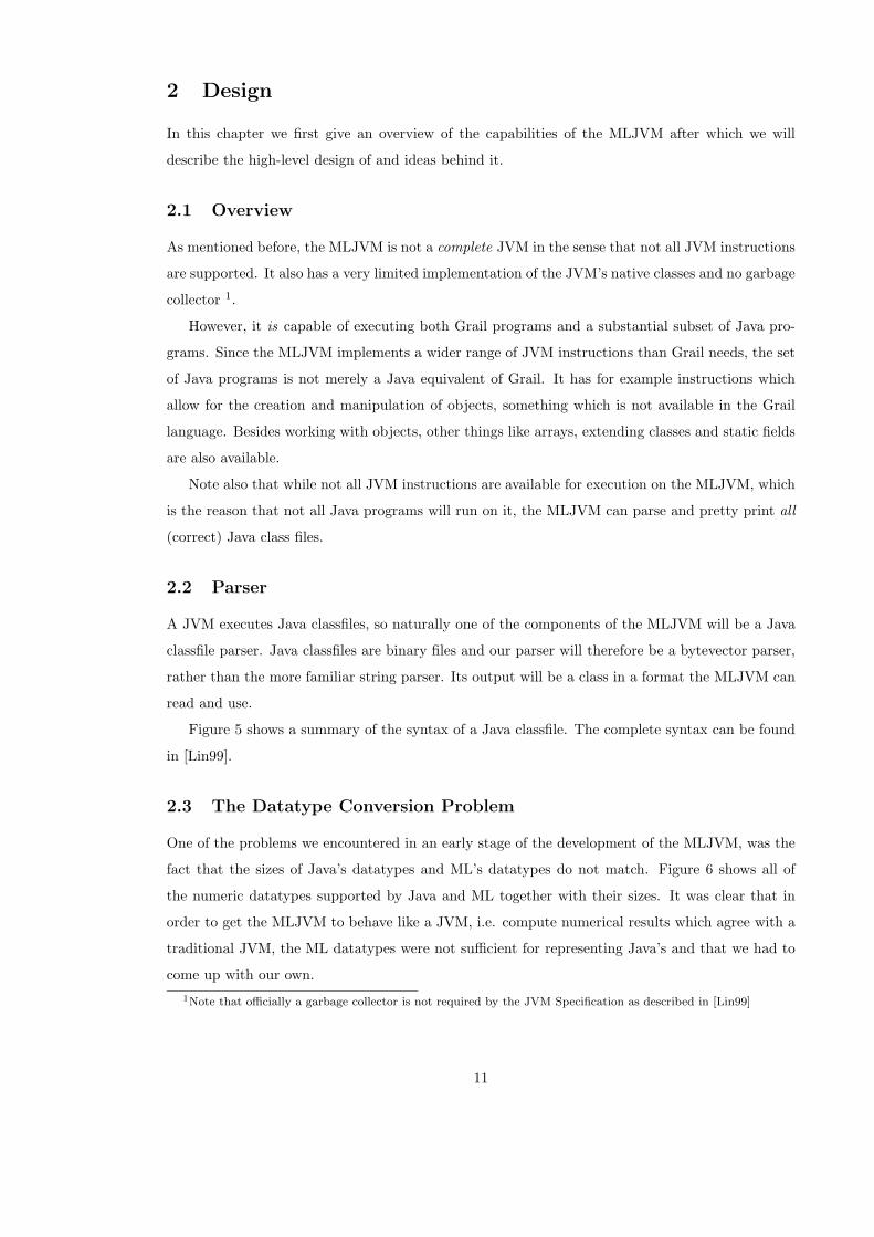
Figure 5 shows a summary of the syntax of a Java classfile. The complete syntax can be found
in [Lin99].
2.3 The Datatype Conversion Problem
One of the problems we encountered in an early stage of the development of the MLJVM, was the
fact that the sizes of Java’s datatypes and ML’s datatypes do not match. Figure 6 shows all of
the numeric datatypes supported by Java and ML together with their sizes. It was clear that in
order to get the MLJVM to behave like a JVM, i.e. compute numerical results which agree with a
traditional JVM, the ML datatypes were not sufficient for representing Java’s and that we had to
come up with our own.
1Note that officially a garbage collector is not required by the JVM Specification as described in [Lin99]
11
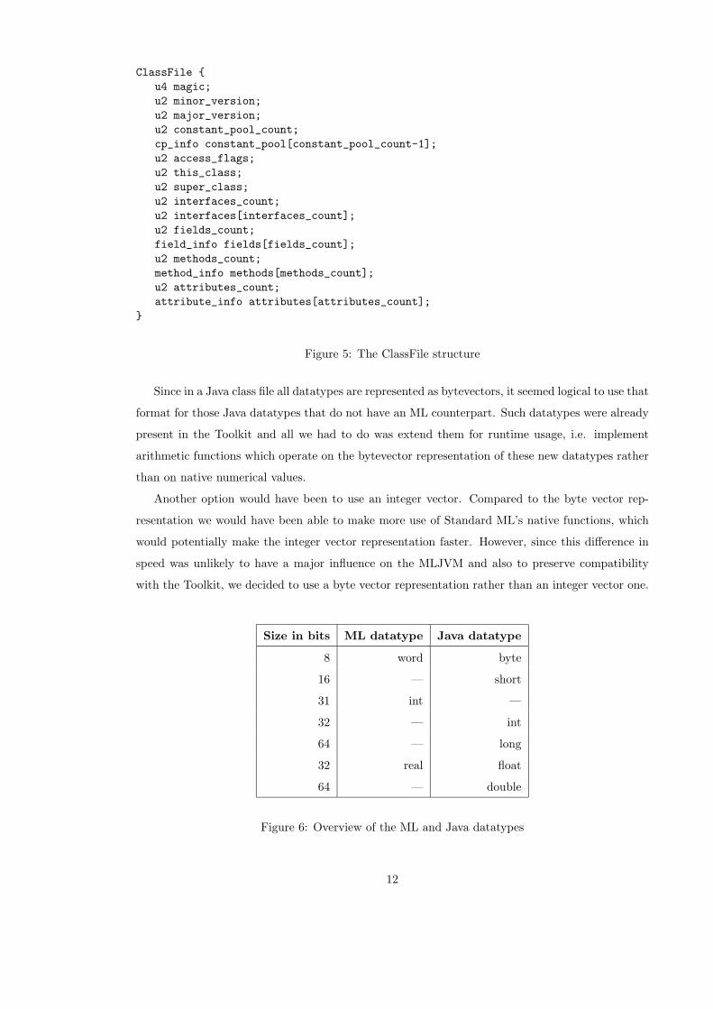
ClassFile {
u4 magic;
u2 minor_version;
u2 major_version;
u2 constant_pool_count;
cp_info constant_pool[constant_pool_count-1];
u2 access_flags;
u2 this_class;
u2 super_class;
u2 interfaces_count;
u2 interfaces[interfaces_count];
u2 fields_count;
field_info fields[fields_count];
u2 methods_count;
method_info methods[methods_count];
u2 attributes_count;
attribute_info attributes[attributes_count];
}
Figure 5: The ClassFile structure
Since in a Java class file all datatypes are represented as bytevectors, it seemed logical to use that
format for those Java datatypes that do not have an ML counterpart. Such datatypes were already
present in the Toolkit and all we had to do was extend them for runtime usage, i.e. implement
arithmetic functions which operate on the bytevector representation of these new datatypes rather
than on native numerical values.
Another option would have been to use an integer vector. Compared to the byte vector rep-
resentation we would have been able to make more use of Standard ML’s native functions, which
would potentially make the integer vector representation faster. However, since this difference in
speed was unlikely to have a major influence on the MLJVM and also to preserve compatibility
with the Toolkit, we decided to use a byte vector representation rather than an integer vector one.
Size in bits ML datatype Java datatype
8 word byte
16 — short
31 int —
32 — int
64 — long
32 real float
64 — double
Figure 6: Overview of the ML and Java datatypes
12
Execute its main method
class
Parser
MLJVMControl
1
5
4
3
6
7
2
1
2
3
5
4
7
6
Store classCreate JVM Environment
User call
Heap StackMethod Area
JVM Environment
MLJVM
Internal MLVJM Call
Look for Java classfile
Read Java classfile
Send class to MLJVM Control
Execute its initialisation method
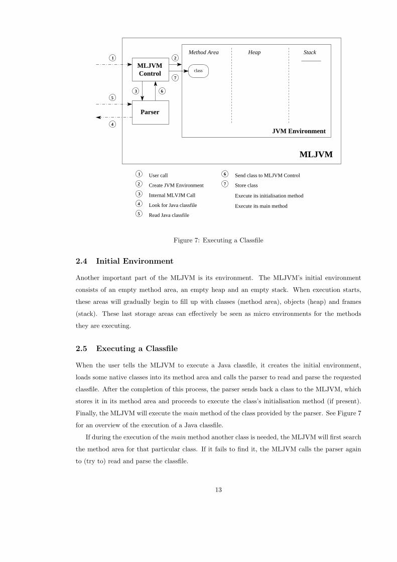
Figure 7: Executing a Classfile
2.4 Initial Environment
Another important part of the MLJVM is its environment. The MLJVM’s initial environment
consists of an empty method area, an empty heap and an empty stack. When execution starts,
these areas will gradually begin to fill up with classes (method area), objects (heap) and frames
(stack). These last storage areas can effectively be seen as micro environments for the methods
they are executing.
2.5 Executing a Classfile
When the user tells the MLJVM to execute a Java classfile, it creates the initial environment,
loads some native classes into its method area and calls the parser to read and parse the requested
classfile. After the completion of this process, the parser sends back a class to the MLJVM, which
stores it in its method area and proceeds to execute the class’s initialisation method (if present).
Finally, the MLJVM will execute the main method of the class provided by the parser. See Figure 7
for an overview of the execution of a Java classfile.
If during the execution of the main method another class is needed, the MLJVM will first search
the method area for that particular class. If it fails to find it, the MLJVM calls the parser again
to (try to) read and parse the classfile.
13
MLJVM
6
4
5
3
2
1
2
6
3
4
5
1
ControlMLJVM
Parser
Print class to standard output
Send class to MLJVM Control
Read Java classfile
Internal MLJVM call
User call
Look for Java classfile
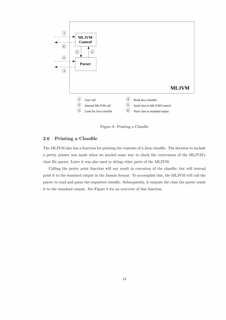
Figure 8: Printing a Classfile
2.6 Printing a Classfile
The MLJVM also has a function for printing the contents of a Java classfile. The decision to include
a pretty printer was made when we needed some way to check the correctness of the MLJVM’s
class file parser. Later it was also used to debug other parts of the MLJVM.
Calling the pretty print function will not result in execution of the classfile, but will instead
print it to the standard output in the Jasmin format. To accomplish this, the MLJVM will call the
parser to read and parse the requested classfile. Subsequently, it outputs the class the parser sends
it to the standard output. See Figure 8 for an overview of this function.
14
3 Implementation
In this chapter we will introduce the implementation of the MLJVM in a little more detail. Besides
revealing the different files the MLJVM is made up of, we will also explain their purpose and
working.
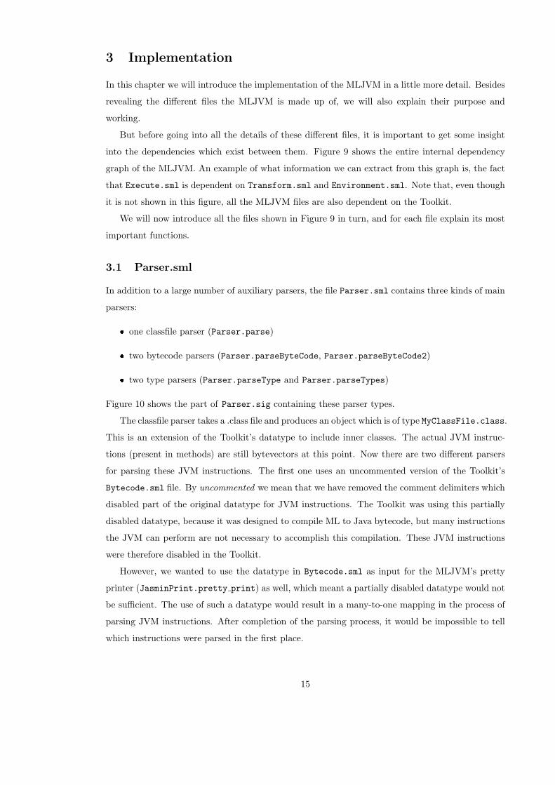
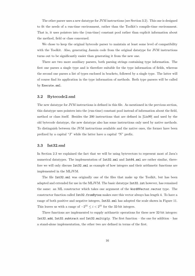
But before going into all the details of these different files, it is important to get some insight
into the dependencies which exist between them. Figure 9 shows the entire internal dependency
graph of the MLJVM. An example of what information we can extract from this graph is, the fact
that Execute.sml is dependent on Transform.sml and Environment.sml. Note that, even though
it is not shown in this figure, all the MLJVM files are also dependent on the Toolkit.
We will now introduce all the files shown in Figure 9 in turn, and for each file explain its most
important functions.
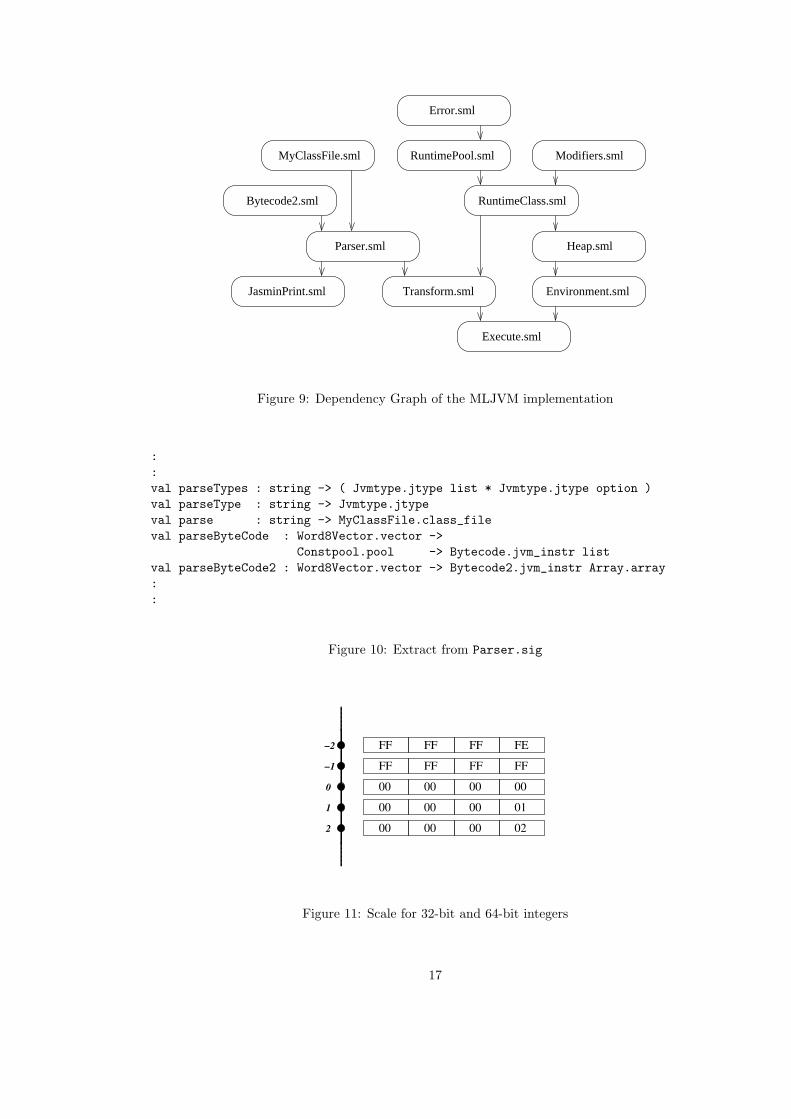
3.1 Parser.sml
In addition to a large number of auxiliary parsers, the file Parser.sml contains three kinds of main
parsers:
� one classfile parser (Parser.parse)
� two bytecode parsers (Parser.parseByteCode, Parser.parseByteCode2)
� two type parsers (Parser.parseType and Parser.parseTypes)
Figure 10 shows the part of Parser.sig containing these parser types.
The classfile parser takes a .class file and produces an object which is of type MyClassFile.class.
This is an extension of the Toolkit’s datatype to include inner classes. The actual JVM instruc-
tions (present in methods) are still bytevectors at this point. Now there are two different parsers
for parsing these JVM instructions. The first one uses an uncommented version of the Toolkit’s
Bytecode.sml file. By uncommented we mean that we have removed the comment delimiters which
disabled part of the original datatype for JVM instructions. The Toolkit was using this partially
disabled datatype, because it was designed to compile ML to Java bytecode, but many instructions
the JVM can perform are not necessary to accomplish this compilation. These JVM instructions
were therefore disabled in the Toolkit.
However, we wanted to use the datatype in Bytecode.sml as input for the MLJVM’s pretty
printer (JasminPrint.pretty print) as well, which meant a partially disabled datatype would not
be sufficient. The use of such a datatype would result in a many-to-one mapping in the process of
parsing JVM instructions. After completion of the parsing process, it would be impossible to tell
which instructions were parsed in the first place.
15
The other parser uses a new datatype for JVM instructions (see Section 3.2). This one is designed
to fit the needs of a run-time environment, rather than the Toolkit’s compile-time environment.
That is, it uses pointers into the (run-time) constant pool rather than explicit information about
the method, field or class concerned.
We chose to keep the original bytecode parser to maintain at least some level of compatibility
with the Toolkit. Also, generating Jasmin code from the original datatype for JVM instructions
turns out to be significantly easier than generating it from the new one.
There are two more auxiliary parsers, both parsing strings containing type information. The
first one parses a single type and is therefore suitable for the type information of fields, whereas
the second one parses a list of types enclosed in brackets, followed by a single type. The latter will
of course find its application in the type information of methods. Both type parsers will be called
by Execute.sml.
3.2 Bytecode2.sml
The new datatype for JVM instructions is defined in this file. As mentioned in the previous section,
this datatype uses pointers into the (run-time) constant pool instead of information about the field,
method or class itself. Besides the 200 instructions that are defined in [Lin99] and used by the
old bytecode datatype, the new datatype also has some instructions only used by native methods.
To distinguish between the JVM instructions available and the native ones, the former have been
prefixed by a capital “J” while the latter have a capital “N” prefix.
3.3 Int32.sml
In Section 2.3 we explained the fact that we will be using bytevectors to represent most of Java’s
numerical datatypes. The implementation of Int32.sml and Int64.sml are rather similar, there-
fore we will only discuss Int32.sml as example of how integers and their arithmetic functions are
implemented in the MLJVM.
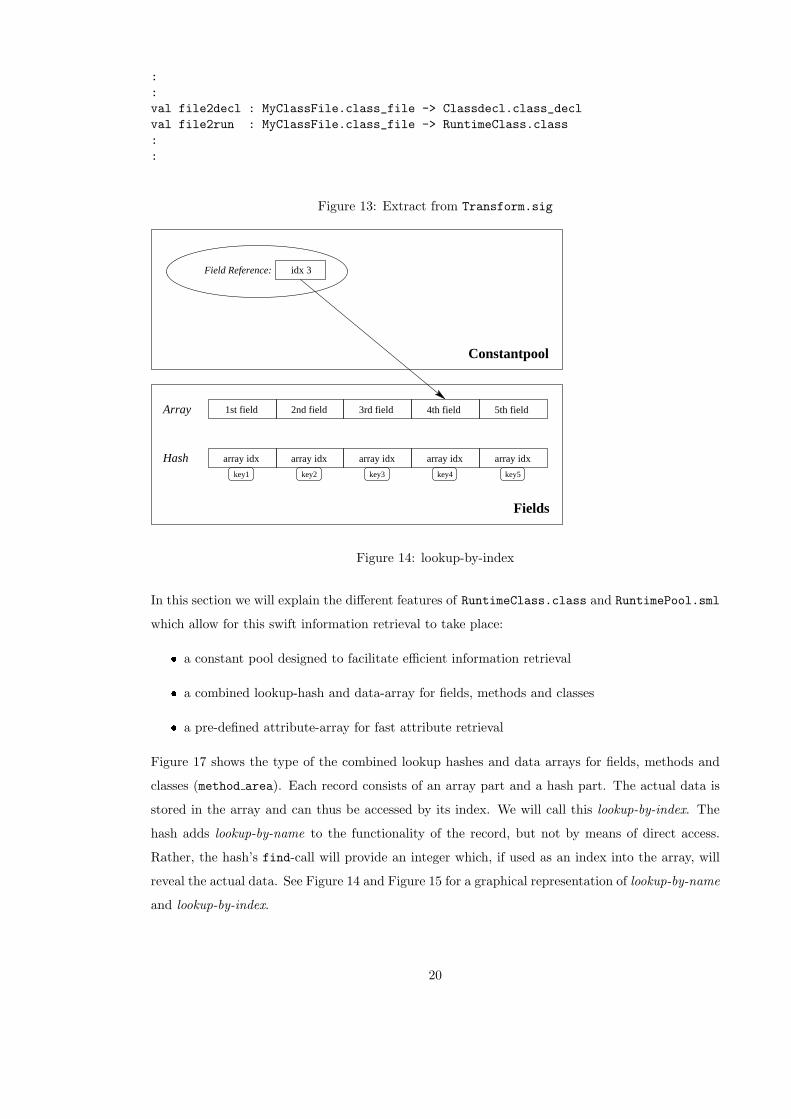
The file Int32.sml was originally one of the files that make up the Toolkit, but has been
adapted and extended for use in the MLJVM. The basic datatype Int32.int however, has remained
the same: an ML constructor which takes one argument of the Word8Vector.vector type. The
constructor function called Int32.fromBytes makes sure this vector always has length 4. To have a
range of both positive and negative integers, Int32.sml has adopted the scale shown in Figure 11.
This leaves us with a range of −231 ≤ i < 231 for the 32-bit integers.
Three functions are implemented to supply arithmetic operations for these new 32-bit integers:
Int32.add, Int32.subtract and Int32.multiply. The first function – the one for addition – has
a stand-alone implementation, the other two are defined in terms of the first.
16
RuntimePool.sml
RuntimeClass.sml
Execute.sml
Transform.sml
MyClassFile.sml
Heap.sml
JasminPrint.sml
Modifiers.sml
Error.sml
Parser.sml
Environment.sml
Bytecode2.sml
Figure 9: Dependency Graph of the MLJVM implementation
:
:
val parseTypes : string -> ( Jvmtype.jtype list * Jvmtype.jtype option )
val parseType : string -> Jvmtype.jtype
val parse : string -> MyClassFile.class_file
val parseByteCode : Word8Vector.vector ->
Constpool.pool -> Bytecode.jvm_instr list
val parseByteCode2 : Word8Vector.vector -> Bytecode2.jvm_instr Array.array
:
:
Figure 10: Extract from Parser.sig
2
FF FF FF FF
00 00 00 00
00 00 0100
00 020000
FF FEFFFF
0
−1
−2
1
Figure 11: Scale for 32-bit and 64-bit integers
17

:
:
fun add (INT w1) (INT w2) =
let val b1 = Word32.toBytes w1
val b2 = Word32.toBytes w2
val l1 = Word8Vector.foldr op:: [] b1
val l2 = Word8Vector.foldr op:: [] b2
val max = Word.fromInt 256
fun f(x,y,(z,c)) =
let val i = Word.+ ( Word.+ ( Word8.toLargeWord x,
Word8.toLargeWord y )
, Word.fromInt c )
in if Word.< (i,max)
then (Word8.fromLargeWord i::z,0)
else (Word8.fromLargeWord i::z,1)
end
val result = (fromBytes o Word8Vector.fromList o #1)
(ListPair.foldr f ([],0) (l1,l2))
in valOf result
end
:
:
Figure 12: add from Int32.sml
The addition function itself is not extremely complicated. One simply folds an addition function
with carry over the bytevector (Figure 12). The subtract function first flips the sign of its second
argument and then adds it to the first. In formulae: sub(x, y) = add(x, flip(y)). And last, the
multiply function takes its second argument and adds that to the multiplication of its first argument
minus one and its second argument. In formulae: mul(x, y) = add(mul(x − 1, y), y).
3.4 MyClassFile.sml
MyClassFile.sml contains a datatype representing a Java class file as described in Section 1.2. This
datatype is the output type of the classfile parser Parser.parse and input to the transformation
function Transform.file2run and the pretty print function JasminPrint.pretty print.
3.5 Transform.sml
The major purpose of Transform.sml is to transform (of course) the output of the classfile parser
into something a little more useful. The necessity for Transform.sml is best illustrated by the fact
that the datatype that is the output of the classfile parser still uses bytevectors to represent the
JVM instructions present in its methods.
In the section about Parser.sml we already recognised the need for two different bytecode
parsers. So as one might expect, these two bytecode parsers do indeed give rise to two different
18

transformers:
� a transformer for producing the Toolkit’s compile-time representation of a class2
(Transform.file2decl)
� a transformer for producing the MLJVM’s run-time representation of a class
(Transform.file2run)
Figure 13 shows the part of Transform.sig containing these two transformer types.
Note that the first transformer is, as far as the MLJVM is concerned, redundant and will play
no role whatsoever in the execution of a classfile. It is in fact only included for completeness and,
as mentioned before, to maintain some level of compatibility with the Toolkit.
Even though the two transformers are very different from each other, there are three similar-
ities worth mentioning: they both turn the JVM instructions present in methods into something
more concrete, they both introduce a datatype (the same) for access flags, and they both use
MyClassFile.class file as their input.
In order to describe their differences, I will first give a brief description of both transformers.
Transform.file2decl produces a compile-time representation of a class. In this representation
there is no constant pool, which means that all information is stored there where one would
usually would find a pointer. Needless to say, this representation could potentially be ex-
tremely inefficient, especially in the case of excessive duplication. However, the information
stored in this datatype is very easy to access, due to a lack of pointer resolution.
Transform.file2run produces the run-time representation of a class. The main features of this
run-time representation are: a constant pool designed to facilitate efficient information re-
trieval, a combined lookup hash and data array for fields, methods and classes, and a pre-
defined attribute array for fast attribute retrieval3.
So even though both transformers hope to make the information represented by the datatype
MyClassFile.class file more accessible (another similarity), they achieve this accessibility in
two very different ways. Where the function Transformer.file2decl replaces its constant pool
and pointers with explicit information, Transformer.file2run creates a network of pointers more
suitable for information retrieval.
3.6 RuntimeClass.sml & RuntimePool.sml
As we saw in the previous section, the transformer Transform.file2run produces something of
type RuntimeClass.class, which was intended to be designed for efficient information retrieval.
2Transform.file2decl actually produces the extended version of the Toolkit’s type. See Section 3.1 for the
reasons behind the decision to extend the Toolkit’s datatype.3See Section 3.6 for further explanation of these features.
19
:
:
val file2decl : MyClassFile.class_file -> Classdecl.class_decl
val file2run : MyClassFile.class_file -> RuntimeClass.class
:
:
Figure 13: Extract from Transform.sig
Fields
Constantpool
Field Reference: idx 3
1st field 2nd field 5th field4th field3rd fieldArray
key1 key4key3 key5key2
array idxarray idxarray idxarray idxarray idxHash
Figure 14: lookup-by-index
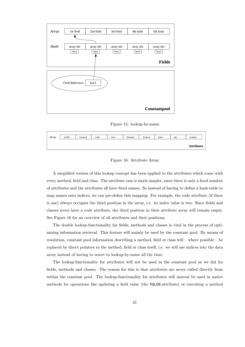
In this section we will explain the different features of RuntimeClass.class and RuntimePool.sml
which allow for this swift information retrieval to take place:
� a constant pool designed to facilitate efficient information retrieval
� a combined lookup-hash and data-array for fields, methods and classes
� a pre-defined attribute-array for fast attribute retrieval
Figure 17 shows the type of the combined lookup hashes and data arrays for fields, methods and
classes (method area). Each record consists of an array part and a hash part. The actual data is
stored in the array and can thus be accessed by its index. We will call this lookup-by-index. The
hash adds lookup-by-name to the functionality of the record, but not by means of direct access.
Rather, the hash’s find-call will provide an integer which, if used as an index into the array, will
reveal the actual data. See Figure 14 and Figure 15 for a graphical representation of lookup-by-name
and lookup-by-index.
20
Fields
key2Field Reference:
1st field 2nd field 5th field4th field3rd fieldArray
key1 key4key3 key5key2
array idxarray idxarray idxarray idxarray idxHash
Constantpool
Figure 15: lookup-by-name
Attributes
Array srcfile constval code exns linenum localvar inner attr (value)
Figure 16: Attribute Array
A simplified version of this lookup concept has been applied to the attributes which come with
every method, field and class. The attribute case is much simpler, since there is only a fixed number
of attributes and the attributes all have fixed names. So instead of having to define a hash-table to
map names onto indices, we can pre-define this mapping. For example, the code attribute (if there
is one) always occupies the third position in the array, i.e. its index value is two. Since fields and
classes never have a code attribute, the third position in their attribute array will remain empty.
See Figure 16 for an overview of all attributes and their positions.
The double lookup-functionality for fields, methods and classes is vital in the process of opti-
mizing information retrieval. This feature will mainly be used by the constant pool. By means of
resolution, constant pool information describing a method, field or class will – where possible – be
replaced by direct pointers to the method, field or class itself, i.e. we will use indices into the data
array instead of having to resort to lookup-by-name all the time.
The lookup-functionality for attributes will not be used in the constant pool as we did for
fields, methods and classes. The reason for this is that attributes are never called directly from
within the constant pool. The lookup-functionality for attributes will instead be used in native
methods for operations like updating a field value (the VALUE-attribute) or executing a method
21

:
:
type class =
{ class_ref : int
, pool : RuntimePool.pool
, flags : Modifiers.access_flag list
, this : RuntimePool.index
, super : RuntimePool.index option
, ifcs : RuntimePool.index list
, fields : { array : (member option) Array.array
, hash : (string, int) Polyhash.hash_table }
, methods : { array : (member option) Array.array
, hash : (string, int) Polyhash.hash_table }
, attrs : attribute Array.array }
type method_area = { array : (class option) Array.array
, hash : (string,int) Polyhash.hash_table }
:
:
Figure 17: Extract from RuntimeClass.sml
(the CODE-attribute).
Apart from the datatype of runtime classes, the (partial) specification of some native classes can
also be found in RuntimeClass.sml. This version of the MLJVM supports (parts of) four native
classes. They are, together with a specification of the implemented parts:
1. java/lang/Object – Implemented Methods: 〈init〉
2. java/io/PrintStream – Implemented Fields: out
3. java/lang/System – Implemented Methods: print, println (both overloaded)
4. java/lang/Integer – Implemented Methods: toString, parseInt
The first one, java/lang/Object which is the superclass of all classes, was added because whenever
an object is being initialised, it also calls its superclass’s initialisation method. The other three
together provide a very basic form of standard output which is vital in the process of debugging
both a Java program and the MLJVM itself.
While it may at first seem easy to implement the JVM’s native classes, because Standard ML
has libraries which do exactly the same, it turns out to be quite a complex task. For this reason,
some of our native functions have only limited functionality compared to Sun’s implementation of
the JVM.
For example the MLJVM output instructions print and println are functional only if used
on the standard output stream out. Implementing the entire PrintStream class would require im-
22
:
:
val pretty_print : MyClassFile.class_file -> unit
:
:
Figure 18: Extract from JasminPrint.sig
plementing the classes OutputStream and FilterOutputStream, facilitating upcasting and down-
casting and providing JVM instructions for write, close and flush functions.
The native classes that have been implemented in the MLJVM are represented in the same way
as user-defined classes. However, while user-defined classes are restricted to the standard set of
JVM instructions to represent the code of their methods, native classes are not. The MLJVM has
an additional set of native instructions which native methods are allowed to use. In the current
implementation of the MLJVM this set consists of the instructions Nprintln, Nprint, Nint2string
and NparseInt.
3.7 Error.sml
Error.sml contains exception information for the entire MLJVM. Some of these exceptions are
generated by functions which have for example the name of the file which generated the exception as
their argument. These exception generating functions are extremely useful for debugging purposes.
3.8 Modifiers.sml
This file contains a datatype for modifiers like public, static or synchronized and some functions
for transforming the words by which the modifiers are represented in the Java class file, into strings
or the new modifier datatype.
3.9 JasminPrint.sml
For debugging purposes the MLJVM needed a pretty printer of some sort. As the format of the
output of the pretty printer, we chose Jasmin because it provides a readable way of representing
class files and can be re-assembled into a binary class file.
Figure 18 shows the input of pretty print to be MyClassFile.class file, which we re-
member to be the output of Parser.parse. At some point, the pretty print function also uses
Parser.parseByteCode, the parser which turns a bytevector into the Toolkit’s datatype for JVM
instructions.
23
3.10 Heap.sml
This version of the MLJVM does not have a garbage collector. However, its heap was designed to
fit the needs of a specific future garbage collector.
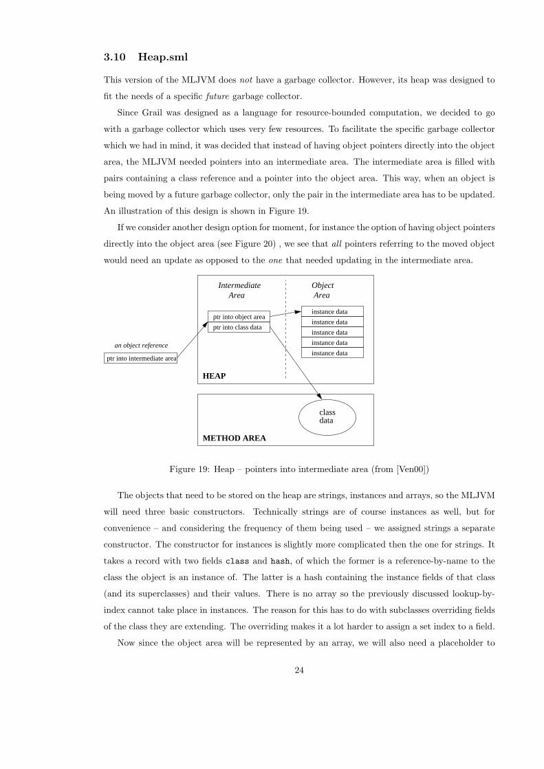
Since Grail was designed as a language for resource-bounded computation, we decided to go
with a garbage collector which uses very few resources. To facilitate the specific garbage collector
which we had in mind, it was decided that instead of having object pointers directly into the object
area, the MLJVM needed pointers into an intermediate area. The intermediate area is filled with
pairs containing a class reference and a pointer into the object area. This way, when an object is
being moved by a future garbage collector, only the pair in the intermediate area has to be updated.
An illustration of this design is shown in Figure 19.
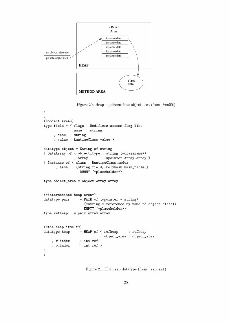
If we consider another design option for moment, for instance the option of having object pointers
directly into the object area (see Figure 20) , we see that all pointers referring to the moved object
would need an update as opposed to the one that needed updating in the intermediate area.
ptr into object area
ptr into intermediate area
dataclass
METHOD AREA
HEAP
AreaObject
AreaIntermediate
an object referenceinstance data
instance data
instance data
instance data
instance data
ptr into class data
Figure 19: Heap – pointers into intermediate area (from [Ven00])
The objects that need to be stored on the heap are strings, instances and arrays, so the MLJVM
will need three basic constructors. Technically strings are of course instances as well, but for
convenience – and considering the frequency of them being used – we assigned strings a separate
constructor. The constructor for instances is slightly more complicated then the one for strings. It
takes a record with two fields class and hash, of which the former is a reference-by-name to the
class the object is an instance of. The latter is a hash containing the instance fields of that class
(and its superclasses) and their values. There is no array so the previously discussed lookup-by-
index cannot take place in instances. The reason for this has to do with subclasses overriding fields
of the class they are extending. The overriding makes it a lot harder to assign a set index to a field.
Now since the object area will be represented by an array, we will also need a placeholder to
24
METHOD AREA
Object
instance data
instance data
instance data
instance data
instance data
classdata
ptr into object area
an object reference
HEAP
Area
Figure 20: Heap – pointers into object area (from [Ven00])
:
:
(*object area*)
type field = { flags : Modifiers.access_flag list
, name : string
, desc : string
, value : RuntimeClass.value }
datatype object = String of string
| DataArray of { object_type : string (*classname*)
, array : hpointer Array.array }
| Instance of { class : RuntimeClass.index
, hash : (string,field) Polyhash.hash_table }
| DUMMY (*placeholder*)
type object_area = object Array.array
(*intermediate heap area*)
datatype pair = PAIR of (opointer * string)
(*string = reference-by-name to object-class*)
| EMPTY (*placeholder*)
type refheap = pair Array.array
(*the heap itself*)
datatype heap = HEAP of { refheap : refheap
, object_area : object_area
, r_index : int ref
, o_index : int ref }
:
:
Figure 21: The heap datatype (from Heap.sml)
25
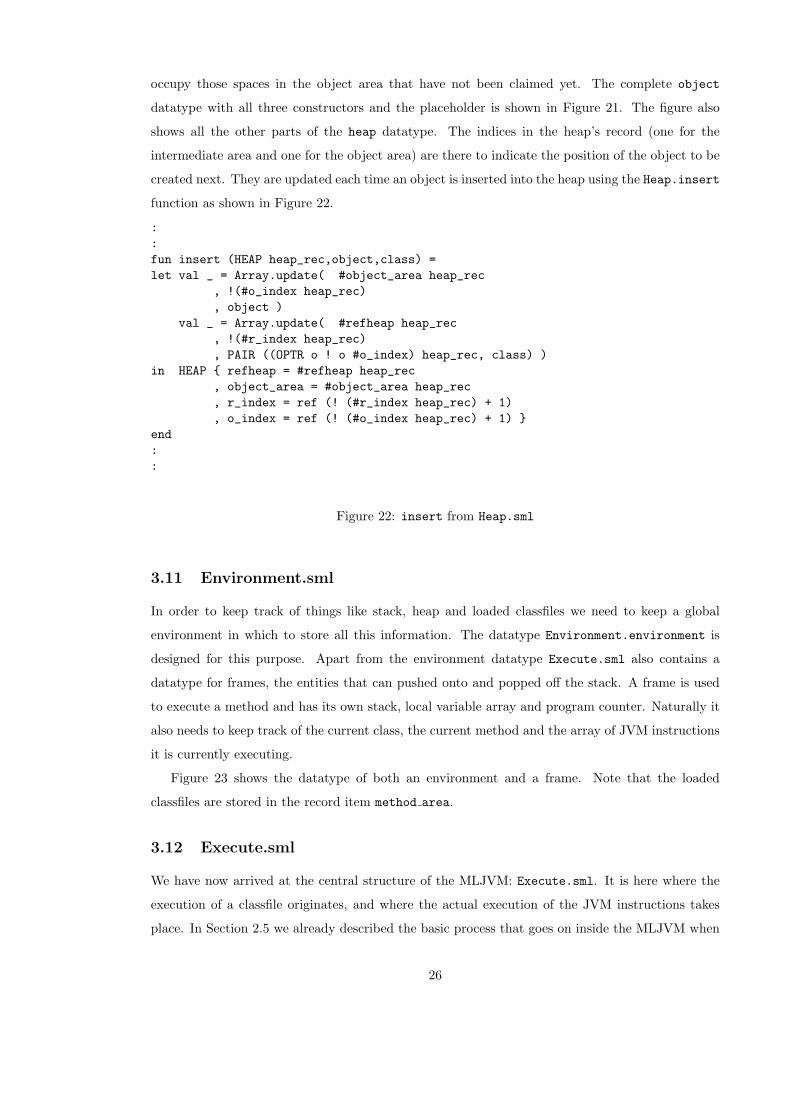
occupy those spaces in the object area that have not been claimed yet. The complete object
datatype with all three constructors and the placeholder is shown in Figure 21. The figure also
shows all the other parts of the heap datatype. The indices in the heap’s record (one for the
intermediate area and one for the object area) are there to indicate the position of the object to be
created next. They are updated each time an object is inserted into the heap using the Heap.insert
function as shown in Figure 22.
:
:
fun insert (HEAP heap_rec,object,class) =
let val _ = Array.update( #object_area heap_rec
, !(#o_index heap_rec)
, object )
val _ = Array.update( #refheap heap_rec
, !(#r_index heap_rec)
, PAIR ((OPTR o ! o #o_index) heap_rec, class) )
in HEAP { refheap = #refheap heap_rec
, object_area = #object_area heap_rec
, r_index = ref (! (#r_index heap_rec) + 1)
, o_index = ref (! (#o_index heap_rec) + 1) }
end
:
:
Figure 22: insert from Heap.sml
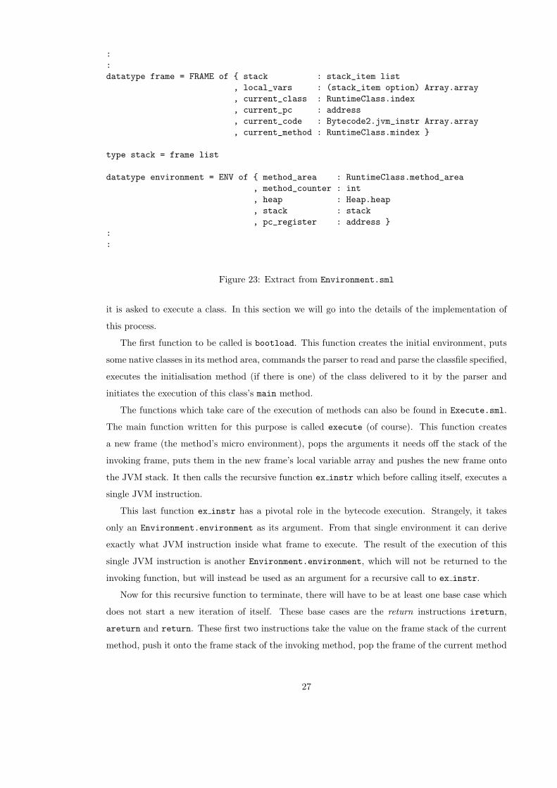
3.11 Environment.sml
In order to keep track of things like stack, heap and loaded classfiles we need to keep a global
environment in which to store all this information. The datatype Environment.environment is
designed for this purpose. Apart from the environment datatype Execute.sml also contains a
datatype for frames, the entities that can pushed onto and popped off the stack. A frame is used
to execute a method and has its own stack, local variable array and program counter. Naturally it
also needs to keep track of the current class, the current method and the array of JVM instructions
it is currently executing.
Figure 23 shows the datatype of both an environment and a frame. Note that the loaded
classfiles are stored in the record item method area.
3.12 Execute.sml
We have now arrived at the central structure of the MLJVM: Execute.sml. It is here where the
execution of a classfile originates, and where the actual execution of the JVM instructions takes
place. In Section 2.5 we already described the basic process that goes on inside the MLJVM when
26
:
:
datatype frame = FRAME of { stack : stack_item list
, local_vars : (stack_item option) Array.array
, current_class : RuntimeClass.index
, current_pc : address
, current_code : Bytecode2.jvm_instr Array.array
, current_method : RuntimeClass.mindex }
type stack = frame list
datatype environment = ENV of { method_area : RuntimeClass.method_area
, method_counter : int
, heap : Heap.heap
, stack : stack
, pc_register : address }
:
:
Figure 23: Extract from Environment.sml
it is asked to execute a class. In this section we will go into the details of the implementation of
this process.
The first function to be called is bootload. This function creates the initial environment, puts
some native classes in its method area, commands the parser to read and parse the classfile specified,
executes the initialisation method (if there is one) of the class delivered to it by the parser and
initiates the execution of this class’s main method.
The functions which take care of the execution of methods can also be found in Execute.sml.
The main function written for this purpose is called execute (of course). This function creates
a new frame (the method’s micro environment), pops the arguments it needs off the stack of the
invoking frame, puts them in the new frame’s local variable array and pushes the new frame onto
the JVM stack. It then calls the recursive function ex instr which before calling itself, executes a
single JVM instruction.
This last function ex instr has a pivotal role in the bytecode execution. Strangely, it takes
only an Environment.environment as its argument. From that single environment it can derive
exactly what JVM instruction inside what frame to execute. The result of the execution of this
single JVM instruction is another Environment.environment, which will not be returned to the
invoking function, but will instead be used as an argument for a recursive call to ex instr.
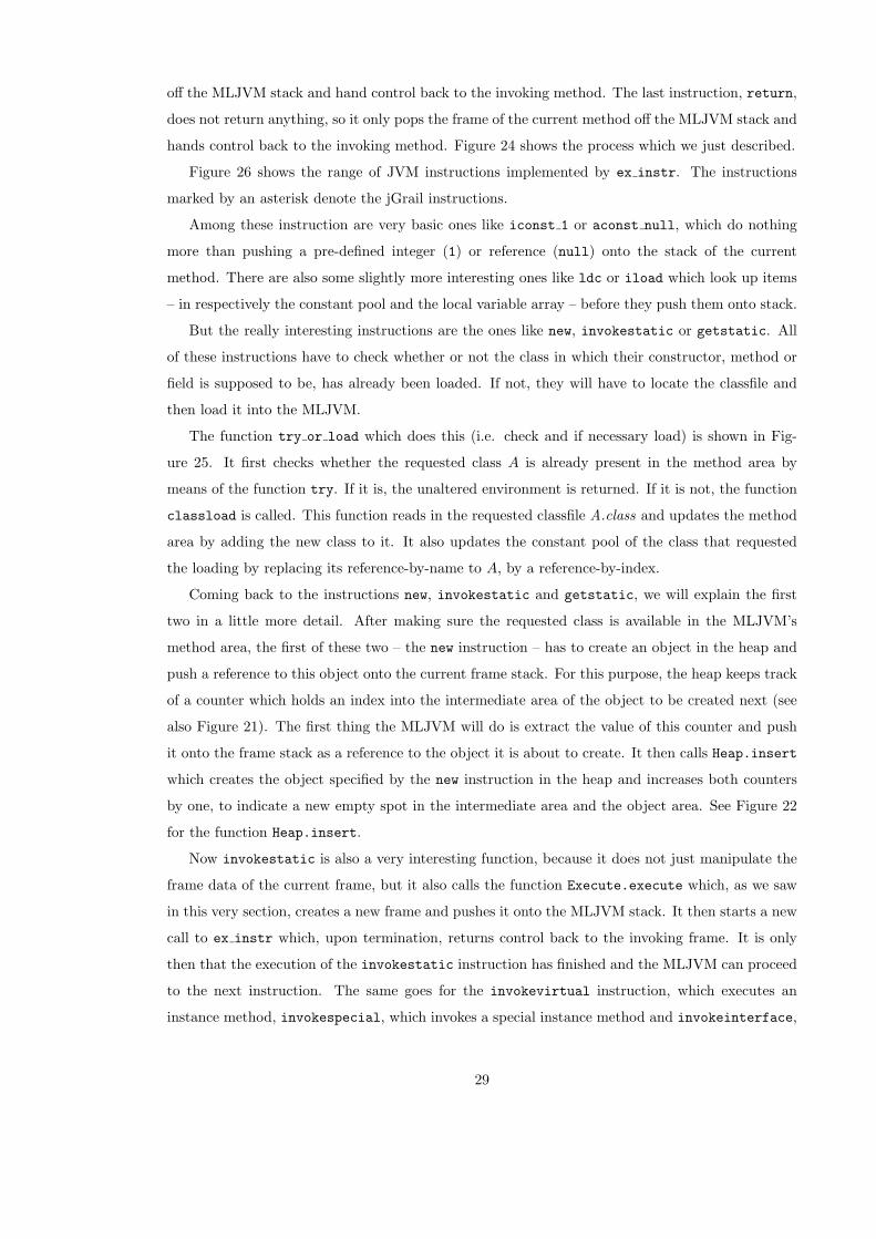
Now for this recursive function to terminate, there will have to be at least one base case which
does not start a new iteration of itself. These base cases are the return instructions ireturn,
areturn and return. These first two instructions take the value on the frame stack of the current
method, push it onto the frame stack of the invoking method, pop the frame of the current method
27

Int
2
0 −
ico
nst
_2
1 −
ico
nst
_3
2 −
in
voke
sta
tic
my_
ad
d(I
I)I
3 −
...
0 −
ilo
ad
_0
1 −
ilo
ad
_1
2 −
ia
dd
3 −
ire
turn
Int
3
Int
2
Int
2
Int
2
Int
3
Int
2
Int
3
Int
5
Int
5
Int
3
Int
2
Int
2
Int
3
FR
AM
EF
RA
ME
FR
AM
EF
RA
ME
FR
AM
E
FR
AM
EF
RA
ME
FR
AM
EF
RA
ME
FR
AM
EF
RA
ME
FR
AM
E
Int
2
Int
3
Figure 24: The MLJVM stack during the invocation of a method
28
off the MLJVM stack and hand control back to the invoking method. The last instruction, return,
does not return anything, so it only pops the frame of the current method off the MLJVM stack and
hands control back to the invoking method. Figure 24 shows the process which we just described.
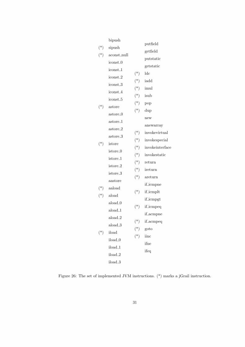
Figure 26 shows the range of JVM instructions implemented by ex instr. The instructions
marked by an asterisk denote the jGrail instructions.
Among these instruction are very basic ones like iconst 1 or aconst null, which do nothing
more than pushing a pre-defined integer (1) or reference (null) onto the stack of the current
method. There are also some slightly more interesting ones like ldc or iload which look up items
– in respectively the constant pool and the local variable array – before they push them onto stack.
But the really interesting instructions are the ones like new, invokestatic or getstatic. All
of these instructions have to check whether or not the class in which their constructor, method or
field is supposed to be, has already been loaded. If not, they will have to locate the classfile and
then load it into the MLJVM.
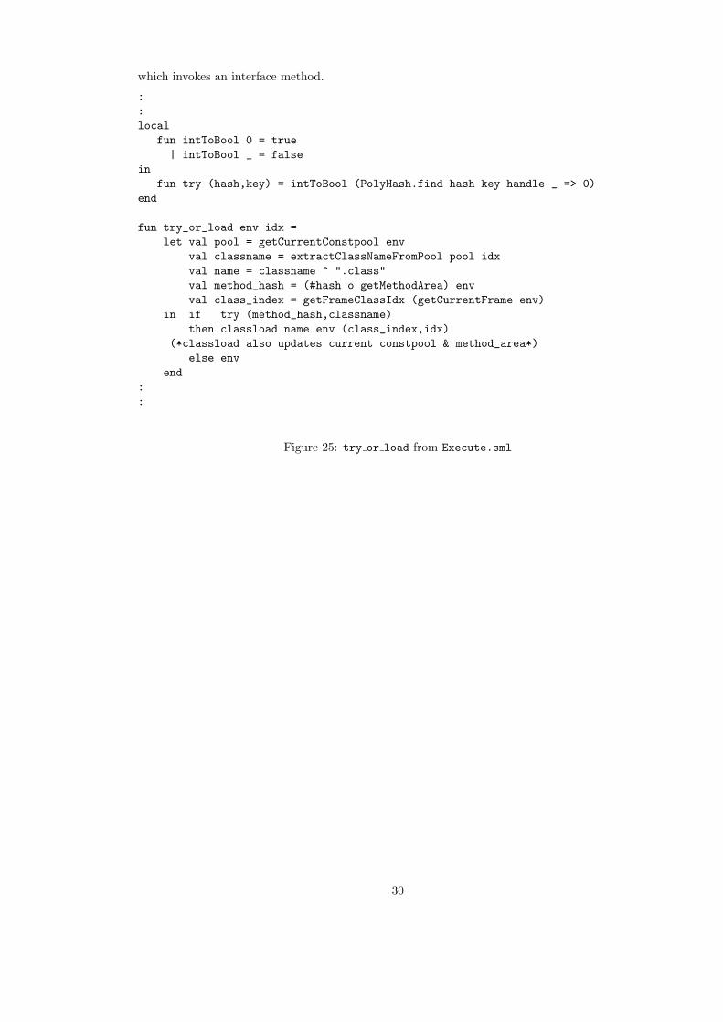
The function try or load which does this (i.e. check and if necessary load) is shown in Fig-
ure 25. It first checks whether the requested class A is already present in the method area by
means of the function try. If it is, the unaltered environment is returned. If it is not, the function
classload is called. This function reads in the requested classfile A.class and updates the method
area by adding the new class to it. It also updates the constant pool of the class that requested
the loading by replacing its reference-by-name to A, by a reference-by-index.
Coming back to the instructions new, invokestatic and getstatic, we will explain the first
two in a little more detail. After making sure the requested class is available in the MLJVM’s
method area, the first of these two – the new instruction – has to create an object in the heap and
push a reference to this object onto the current frame stack. For this purpose, the heap keeps track
of a counter which holds an index into the intermediate area of the object to be created next (see
also Figure 21). The first thing the MLJVM will do is extract the value of this counter and push
it onto the frame stack as a reference to the object it is about to create. It then calls Heap.insert
which creates the object specified by the new instruction in the heap and increases both counters
by one, to indicate a new empty spot in the intermediate area and the object area. See Figure 22
for the function Heap.insert.
Now invokestatic is also a very interesting function, because it does not just manipulate the
frame data of the current frame, but it also calls the function Execute.execute which, as we saw
in this very section, creates a new frame and pushes it onto the MLJVM stack. It then starts a new
call to ex instr which, upon termination, returns control back to the invoking frame. It is only
then that the execution of the invokestatic instruction has finished and the MLJVM can proceed
to the next instruction. The same goes for the invokevirtual instruction, which executes an
instance method, invokespecial, which invokes a special instance method and invokeinterface,
29
which invokes an interface method.
:
:
local
fun intToBool 0 = true
| intToBool _ = false
in
fun try (hash,key) = intToBool (PolyHash.find hash key handle _ => 0)
end
fun try_or_load env idx =
let val pool = getCurrentConstpool env
val classname = extractClassNameFromPool pool idx
val name = classname ^ ".class"
val method_hash = (#hash o getMethodArea) env
val class_index = getFrameClassIdx (getCurrentFrame env)
in if try (method_hash,classname)
then classload name env (class_index,idx)
(*classload also updates current constpool & method_area*)
else env
end
:
:
Figure 25: try or load from Execute.sml
30
bipush
(*) sipush
(*) aconst null
iconst 0
iconst 1
iconst 2
iconst 3
iconst 4
iconst 5
(*) astore
astore 0
astore 1
astore 2
astore 3
(*) istore
istore 0
istore 1
istore 2
istore 3
aastore
(*) aaload
(*) aload
aload 0
aload 1
aload 2
aload 3
(*) iload
iload 0
iload 1
iload 2
iload 3
putfield
getfield
putstatic
getstatic
(*) ldc
(*) iadd
(*) imul
(*) isub
(*) pop
(*) dup
new
anewarray
(*) invokevirtual
(*) invokespecial
(*) invokeinterface
(*) invokestatic
(*) return
(*) ireturn
(*) areturn
if icmpne
(*) if icmplt
if icmpgt
(*) if icmpeq
if acmpne
(*) if acmpeq
(*) goto
(*) iinc
ifne
ifeq
Figure 26: The set of implemented JVM instructions. (*) marks a jGrail instruction.
31
4 Running the MLJVM on some examples
4.1 Example 1 – Parsing a Method Type
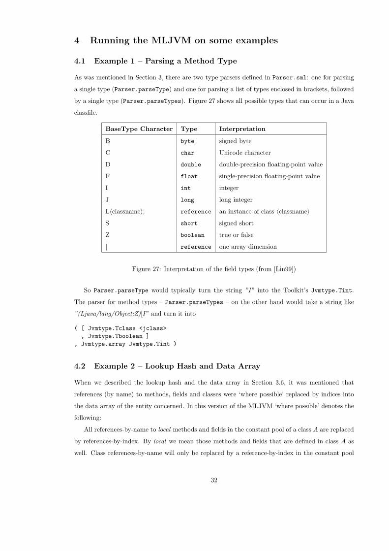
As was mentioned in Section 3, there are two type parsers defined in Parser.sml: one for parsing
a single type (Parser.parseType) and one for parsing a list of types enclosed in brackets, followed
by a single type (Parser.parseTypes). Figure 27 shows all possible types that can occur in a Java
classfile.
BaseType Character Type Interpretation
B byte signed byte
C char Unicode character
D double double-precision floating-point value
F float single-precision floating-point value
I int integer
J long long integer
L〈classname〉; reference an instance of class 〈classname〉
S short signed short
Z boolean true or false
[ reference one array dimension
Figure 27: Interpretation of the field types (from [Lin99])
So Parser.parseType would typically turn the string ”I” into the Toolkit’s Jvmtype.Tint.
The parser for method types – Parser.parseTypes – on the other hand would take a string like
”(Ljava/lang/Object;Z)[I” and turn it into
( [ Jvmtype.Tclass <jclass>
, Jvmtype.Tboolean ]
, Jvmtype.array Jvmtype.Tint )
4.2 Example 2 – Lookup Hash and Data Array
When we described the lookup hash and the data array in Section 3.6, it was mentioned that
references (by name) to methods, fields and classes were ‘where possible’ replaced by indices into
the data array of the entity concerned. In this version of the MLJVM ‘where possible’ denotes the
following:
All references-by-name to local methods and fields in the constant pool of a class A are replaced
by references-by-index. By local we mean those methods and fields that are defined in class A as
well. Class references-by-name will only be replaced by a reference-by-index in the constant pool
32
class SomeClass {
public static void a() {}
public static void b() {}
public static void c() {}
public static void main(String args[]) {
a(); b(); c(); SomeOtherClass.d();
}
}
Figure 28: Java File
of the class that requested the loading of that particular class. However, in the future we would
also like to replace a reference-by-name with a reference-by-index in the constant pool of a class A
whenever a field, method or class is called for the first time by this class A.
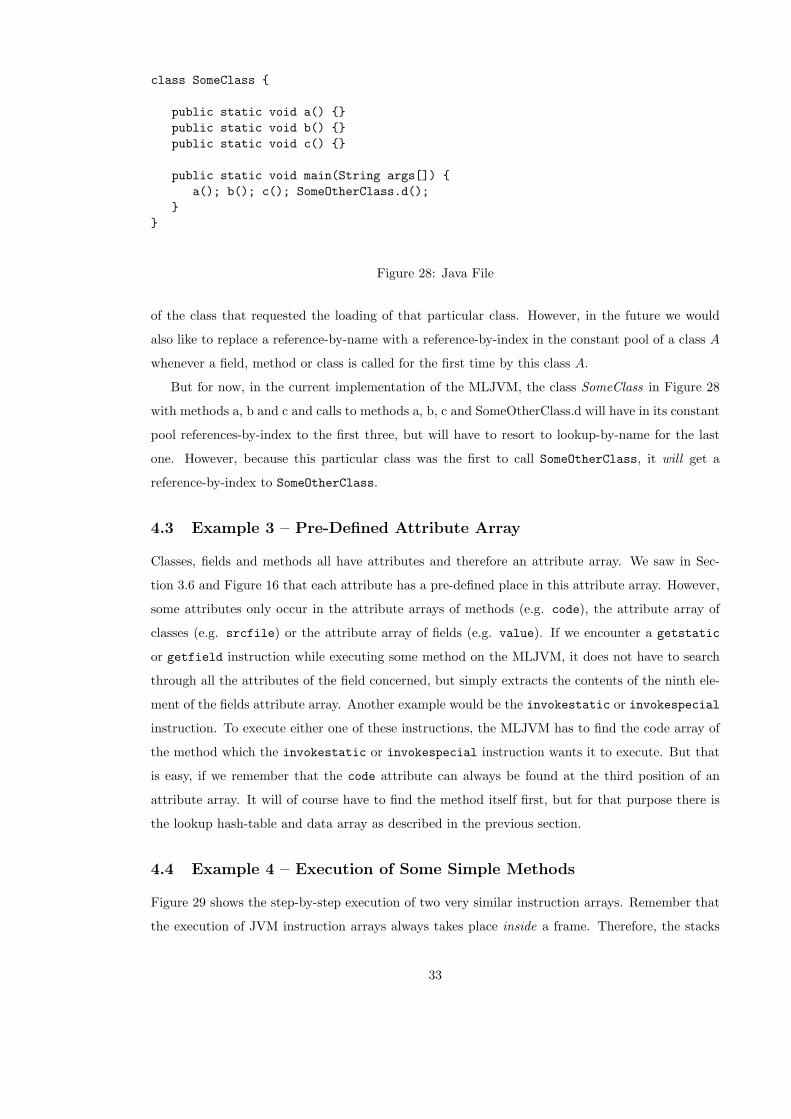
But for now, in the current implementation of the MLJVM, the class SomeClass in Figure 28
with methods a, b and c and calls to methods a, b, c and SomeOtherClass.d will have in its constant
pool references-by-index to the first three, but will have to resort to lookup-by-name for the last
one. However, because this particular class was the first to call SomeOtherClass, it will get a
reference-by-index to SomeOtherClass.
4.3 Example 3 – Pre-Defined Attribute Array
Classes, fields and methods all have attributes and therefore an attribute array. We saw in Sec-
tion 3.6 and Figure 16 that each attribute has a pre-defined place in this attribute array. However,
some attributes only occur in the attribute arrays of methods (e.g. code), the attribute array of
classes (e.g. srcfile) or the attribute array of fields (e.g. value). If we encounter a getstatic
or getfield instruction while executing some method on the MLJVM, it does not have to search
through all the attributes of the field concerned, but simply extracts the contents of the ninth ele-
ment of the fields attribute array. Another example would be the invokestatic or invokespecial
instruction. To execute either one of these instructions, the MLJVM has to find the code array of
the method which the invokestatic or invokespecial instruction wants it to execute. But that
is easy, if we remember that the code attribute can always be found at the third position of an
attribute array. It will of course have to find the method itself first, but for that purpose there is
the lookup hash-table and data array as described in the previous section.
4.4 Example 4 – Execution of Some Simple Methods
Figure 29 shows the step-by-step execution of two very similar instruction arrays. Remember that
the execution of JVM instruction arrays always takes place inside a frame. Therefore, the stacks
33
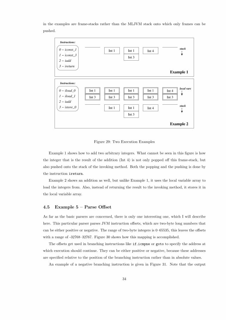
in the examples are frame-stacks rather than the MLJVM stack onto which only frames can be
pushed.
Example 2
Int 1 Int 4
Int 3
Int 1stack0 − iconst_1
1 − iconst_3
2 − iadd
3 − ireturn
Instructions:
Example 1
Int 1
Int 3 Int 3
Int 1
Int 3
Int 1
Int 3
Int 1 Int 4
Int 3
Int 3
Int 1 Int 4Int 1
local vars
stack
0 − iload_0
1 − iload_1
2 − iadd
3 − istore_0
Instructions:
Figure 29: Two Execution Examples
Example 1 shows how to add two arbitrary integers. What cannot be seen in this figure is how
the integer that is the result of the addition (Int 4) is not only popped off this frame-stack, but
also pushed onto the stack of the invoking method. Both the popping and the pushing is done by
the instruction ireturn.
Example 2 shows an addition as well, but unlike Example 1, it uses the local variable array to
load the integers from. Also, instead of returning the result to the invoking method, it stores it in
the local variable array.
4.5 Example 5 – Parse Offset
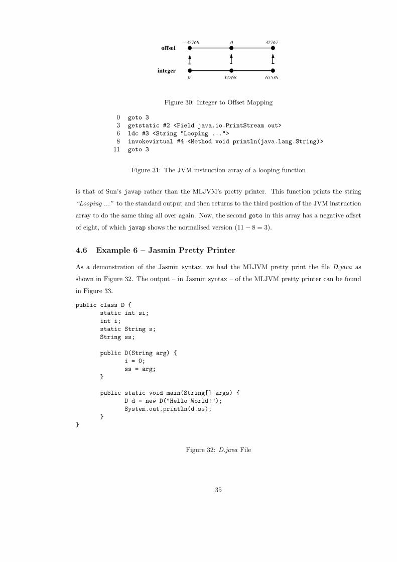
As far as the basic parsers are concerned, there is only one interesting one, which I will describe
here. This particular parser parses JVM instruction offsets, which are two-byte long numbers that
can be either positive or negative. The range of two-byte integers is 0–65535, this leaves the offsets
with a range of -32768–32767. Figure 30 shows how this mapping is accomplished.
The offsets get used in branching instructions like if icmpne or goto to specify the address at
which execution should continue. They can be either positive or negative, because these addresses
are specified relative to the position of the branching instruction rather than in absolute values.
An example of a negative branching instruction is given in Figure 31. Note that the output
34
−32768 32767
offset
integer
0
32768 655360
Figure 30: Integer to Offset Mapping
0 goto 3
3 getstatic #2 <Field java.io.PrintStream out>
6 ldc #3 <String "Looping ...">
8 invokevirtual #4 <Method void println(java.lang.String)>
11 goto 3
Figure 31: The JVM instruction array of a looping function
is that of Sun’s javap rather than the MLJVM’s pretty printer. This function prints the string
“Looping ...” to the standard output and then returns to the third position of the JVM instruction
array to do the same thing all over again. Now, the second goto in this array has a negative offset
of eight, of which javap shows the normalised version (11 − 8 = 3).
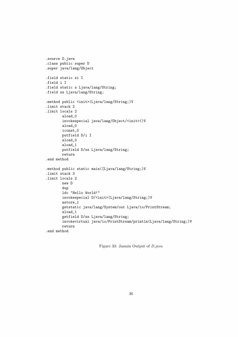
4.6 Example 6 – Jasmin Pretty Printer
As a demonstration of the Jasmin syntax, we had the MLJVM pretty print the file D.java as
shown in Figure 32. The output – in Jasmin syntax – of the MLJVM pretty printer can be found
in Figure 33.
public class D {
static int si;
int i;
static String s;
String ss;
public D(String arg) {
i = 0;
ss = arg;
}
public static void main(String[] args) {
D d = new D("Hello World!");
System.out.println(d.ss);
}
}
Figure 32: D.java File
35
.source D.java
.class public super D
.super java/lang/Object
.field static si I
.field i I
.field static s Ljava/lang/String;
.field ss Ljava/lang/String;
.method public <init>(Ljava/lang/String;)V
.limit stack 2
.limit locals 2
aload_0
invokespecial java/lang/Object/<init>()V
aload_0
iconst_0
putfield D/i I
aload_0
aload_1
putfield D/ss Ljava/lang/String;
return
.end method
.method public static main([Ljava/lang/String;)V
.limit stack 3
.limit locals 2
new D
dup
ldc "Hello World!"
invokespecial D/<init>(Ljava/lang/String;)V
astore_1
getstatic java/lang/System/out Ljava/io/PrintStream;
aload_1
getfield D/ss Ljava/lang/String;
invokevirtual java/io/PrintStream/println(Ljava/lang/String;)V
return
.end method
Figure 33: Jasmin Output of D.java
36
4.7 Example 7 – About Superclasses
Subclasses can be created in a Java program by means of the extends keyword. After compilation
each Java class stores its superclass. The only exception to this rule is the class java/lang/Object,
which is the only class without a superclass. If for any other class no superclass is specified using
the extends keyword, it will be assigned java/lang/Object as its superclass.
In class A all fields, methods and constructors of its superclass B are available, except for the
ones that have been overridden by A. Furthermore, A may specify additional fields, methods and
constructors.
Now if class A would want to call a static method m in B that has not been overridden, it
can simply use the method name m. The compiler will turn this method name into the complete
address B.m before using it in one of the JVM instructions. Something similar happens when class
A would like to call a static field in B.
However, the compiler does not specify the complete address when A wants to call an instance
method i in B. Instead, the compiler uses the regular method name i in its JVM instructions and
leaves the task of locating i to the JVM. In practice this means that the MLJVM will first have to
look for the method i in class where it was called from, A. Should this fail, it will go on to look
for i in the superclass of A: B. If i is not a method in B either, it will go even further up in the
hierarchy. This process only stops when the JVM either finds i, or arrives at java/lang/Object,
which does not have a superclass. In the latter case the MLJVM will throw an exception because
it was unable to locate the instance method.
Calling an instance field is quite different from any of the previous calls, because they were all
searching for entities that could be found inside a class, in the method area. But unlike instance
methods, static methods and static fields, instance fields are part of an instance and will therefore
be found in the heap rather than in the method area. Because the fields of an instance are arranged
in a hierarchy, the MLJVM does not have to know in which class the instance field was specified.
All it needs is the name and type of the field that is called and the heap position of the instance.
That leaves the creation of an instance to be discussed. If class A with superclass B wants to
create an instance of itself, it will have to go through all of its superclasses to extract the instance
fields. Furthermore, it will have to override fields that are defined more than once and set them all
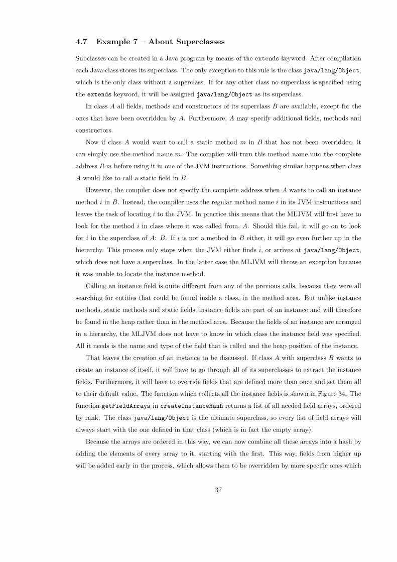
to their default value. The function which collects all the instance fields is shown in Figure 34. The
function getFieldArrays in createInstanceHash returns a list of all needed field arrays, ordered
by rank. The class java/lang/Object is the ultimate superclass, so every list of field arrays will
always start with the one defined in that class (which is in fact the empty array).
Because the arrays are ordered in this way, we can now combine all these arrays into a hash by
adding the elements of every array to it, starting with the first. This way, fields from higher up
will be added early in the process, which allows them to be overridden by more specific ones which
37
:
:
and createInstanceHash env i =
let val instanceHash = Polyhash.mkPolyTable (100, find_error "instance_hash")
fun f x = let val y = valOf x
in Polyhash.insert instanceHash (#name y ^ #desc y, y)
end
fun createInstanceHash’ x = Array.app f x
val (arrays,new_env) = getFieldArrays env (RuntimeClass.IDX i)
val _ = List.app createInstanceHash’ arrays
in (instanceHash,new_env)
end
and getInstanceFields env i =
let val (new_hash,new_env) = createInstanceHash env i
in ( { class = RuntimeClass.IDX i
, hash = new_hash }
, new_env )
end
:
:
Figure 34: getInstanceFields from Execute.sml
are added to the hash at a later stage.
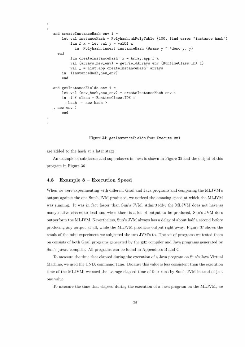
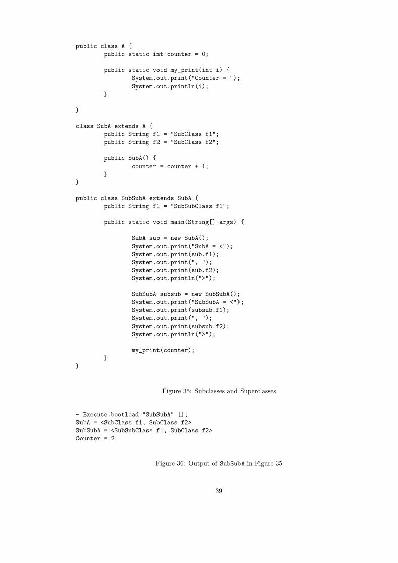
An example of subclasses and superclasses in Java is shown in Figure 35 and the output of this
program in Figure 36
4.8 Example 8 – Execution Speed
When we were experimenting with different Grail and Java programs and comparing the MLJVM’s
output against the one Sun’s JVM produced, we noticed the amazing speed at which the MLJVM
was running. It was in fact faster than Sun’s JVM. Admittedly, the MLJVM does not have as
many native classes to load and when there is a lot of output to be produced, Sun’s JVM does
outperform the MLJVM. Nevertheless, Sun’s JVM always has a delay of about half a second before
producing any output at all, while the MLJVM produces output right away. Figure 37 shows the
result of the mini experiment we subjected the two JVM’s to. The set of programs we tested them
on consists of both Grail programs generated by the gdf compiler and Java programs generated by
Sun’s javac compiler. All programs can be found in Appendices B and C.
To measure the time that elapsed during the execution of a Java program on Sun’s Java Virtual
Machine, we used the UNIX command time. Because this value is less consistent than the execution
time of the MLJVM, we used the average elapsed time of four runs by Sun’s JVM instead of just
one value.
To measure the time that elapsed during the execution of a Java program on the MLJVM, we
38
public class A {
public static int counter = 0;
public static void my_print(int i) {
System.out.print("Counter = ");
System.out.println(i);
}
}
class SubA extends A {
public String f1 = "SubClass f1";
public String f2 = "SubClass f2";
public SubA() {
counter = counter + 1;
}
}
public class SubSubA extends SubA {
public String f1 = "SubSubClass f1";
public static void main(String[] args) {
SubA sub = new SubA();
System.out.print("SubA = <");
System.out.print(sub.f1);
System.out.print(", ");
System.out.print(sub.f2);
System.out.println(">");
SubSubA subsub = new SubSubA();
System.out.print("SubSubA = <");
System.out.print(subsub.f1);
System.out.print(", ");
System.out.print(subsub.f2);
System.out.println(">");
my_print(counter);
}
}
Figure 35: Subclasses and Superclasses
- Execute.bootload "SubSubA" [];
SubA = <SubClass f1, SubClass f2>
SubSubA = <SubSubClass f1, SubClass f2>
Counter = 2
Figure 36: Output of SubSubA in Figure 35
39

Command Sun’s JVM MLJVMHelloWorld 411 1ExThree 45 405 3SumList 123 456 789 422 4SumList 123 456 789 123 456 789 424 5SumList 1 2 3 4 5 6 7 8 9 430 6ExTwo 427 6Q3 436 8Fib 10 420 8Fib 30 425 14ExOne 443 18
Figure 37: Results of the Execution Speed Experiment in Milliseconds
used the ML library structures Timer and Time to create the following function:
fun tex file args =
let val tr = Timer.startRealTimer ()
val env = bootload file args
in Time.toMilliseconds (Timer.checkRealTimer tr)
end
4.9 Example 9 – Generating Exceptions
Of course the MLJVM should not only execute working Java programs correctly, it should also give
a proper response when it is presented with a faulty one. An example of a faulty program is for
example a single class in which no main method is specified:
public class NoMain {}
When the user commands Sun’s JVM to execute this file, it will not be able to find a main method
to execute in the class NoMain or any of its superclasses and therefore fail by writing the following
error message to the standard output:
Shell> java NoMain
Exception in thread "main" java.lang.NoSuchMethodError: main
The MLJVM only has a single thread, so mentioning the thread which produced the error message
would be redundant. It does however give a more specific description of the method that could not
be found, by giving not only the name of the method, but also, the class in which it was supposed
to be present and the type of the method. In the case of main this additional information may
not be very informative, but when confronted with a overloaded method or one that is defined in
more than one class, the information could prove to be very useful for debugging Java class files.
The error message the MLJVM writes to the standard output when it is commanded to execute
the program NoMain is printed below:
- Execute.bootload "NoMain.class" [];
! Uncaught exception:
! NoSuchMethodError "NoMain.main([Ljava/lang/String;)V"
40

Another example of a possible error that may occur when the MLJVM is executing a Java
program, is the absence of a static field. It is true that the validity of every static field is checked
compile-time by the compiler, which certainly reduces the possibility if an error like this occurring
run-time, but it is not impossible to reference a non-existing static field. Figure 38 for example
public class P1 {
public static int counter = 55;
}
public class P2 {
public static void main(String[] args) {
System.out.println(P1.counter);
}
}
Figure 38: Classes P1 and P2
shows two classes P1 and P2. When P2 is compiled after P1, the compiler will succeed when checking
the existence of P1.counter. But if the line specifying the counter would now be removed from the
file containing P1 and P1 would be recompiled, we have made the Java program P2 useless. When
presented with it, Sun’s JVM outputs the following:
Shell> java P2
Exception in thread "main" java.lang.NoSuchFieldError: counter
at P2.main(P2.java:4)
Again, the MLJVM has only one thread, so no need to have it mention it in the error message. It
also does not support linenumber tables, which means it will be unable to produce any statements
about the location of the error in the source file. It does however specify the exact field that is
missing:
- Execute.bootload "P2.class" [];
! Uncaught exception:
! NoSuchFieldError "P1.counterI"
The errors generated by the MLJVM can be found in Error.sml which also includes error datatypes
and functions for debugging the MLJVM itself.
4.10 Example 10 – Debugging the MLJVM
To debug the MLJVM we designed a specific function which will remain part of the code, because the
MLJVM is a work in progress. This way, it will be available for future extensions and improvements
of the MLJVM. The example given in this section concerns the debugging function of Execute.sml.
Other structures have similar debugging functions.
41

The debugging function in Execute.sml takes two arguments: an integer and a string. The
integer indicates which debugging group (e.g. field extraction, method invocation) the debugging
statement belongs to and the string is the output that will be generated by the debugger. The
major advantage of this design is that the user can select exactly what debugging information he
or she needs, without turning the unwanted debug statements into comments. To switch off a
particular debugging group, for example debugging group five, simply add the statement
5 => ()
to the function do debug in Figure 39. To switch the group back on, all the user has to do is remove
the statement or enclose it in comment delimiters. Any integer except ten 4 which is not explicitly
excluded from the debugging process, generates output, so creating a new group only requires the
user to pick such a number which is not yet in use.
As can be seen in Figure 39, the debugging function prints the string which it received as
its second argument and flushes the standard output immediately afterwards. This flushing is
necessary to allow the debugging function to generate output even if the MLJVM should throw
an exception. By default, the output is collected and written to the screen after the execution of
an ML program successfully terminates. Of course no successful termination will ever be reached
when the program throws an exception, which means no output will be written to the screen either.
However, flushing the output stream causes the program to write output to the screen immediately.
To debug the MLJVM we were dependent on this way of debugging, because unlike a language
like Java, the exceptions generated by ML are not very specific. ML only outputs the topmost
exception to the standard output, whereas Java for example generates detailed nested error mes-
sages. That is, the Java compiler does not only tell the user which thread threw the error, but
also which function inside that thread and which instruction inside that function. Furthermore,
the Java compiler also mentions in which Java file and at which line the faulty instruction was
specified. ML on the other hand would only show the error message of the topmost exception.
Standard ML does of course support the possibility of creating specific and even nested excep-
tions yourself, but for the amount of detail we required this was not an option, because the exception
statements would severely obscure our code. The few exceptions and exception generating functions
that we did use to debug the MLJVM can be found in Error.sml.
Furthermore, because nested functions can be defined in ML, there are often a large amount
of variables in scope. If one variable is mistaken for another, ML will usually produce an error
message, except when both variables are of the same type. An example of such an error which
is commonly overlooked is a function with counter inside another function with its own counter.
Because the counters are both integers and both in scope, ML will not produce an error message if
one of the counters is used where the other was expected – the program remains type-correct. We
4Because it is reserved for standard output generated by the Java program running on the MLJVM
42

came across a few of these mix-ups during the creation of the MLJVM. These incidents would be
far more unlikely to happen in languages like C, C++ or Java simply because they do not support
nested functions.
On a more positive note, in Standard ML one can write very large programs without specifying
a single type and still have type-safety that exceeds the type-safety of Java, while in the latter
(almost) every type has to be specified explicitly. So even though the type-error generators of ML
and Java are equally useful, the ML type-checker is more powerful.
Coming back to the debugging function itself, Figure 39 shows that there is a global variable
no debugging which is assigned its final value by the bootload’ function. This boolean reference
indicates whether or not any debugging information should be generated at all. The default function
for executing a Java program bootload calls bootload’ with true as its final argument. This means
it will not generate debugging information. If the user wishes to execute a Java program and output
debugging information from the MLJVM as well, the function bootload’ should be called with
false as its final argument.
Note also that the output generated by the Java program the MLJVM is executing, is handled
by the do debug function as well. The native JVM instructions Nprint and Nprinln both call the
debugging function. The group number they use is 10. The decision to recycle the debugging func-
tion was based on the observation that the JVM’s defined behaviour considering standard output
matches the behaviour of our debugger exactly: it should write output to the screen immediately,
and not wait for successful completion of the program being executed.
One minor implication of having a multi-functional debugging function is that the integer 10
cannot be used for debugging anymore. However, there are 1073741823 other integers to choose
from, so it will not limit the debugging function in any way.
43

:
:
val no_debugging = ref true
fun do_debug n ss = if !no_debugging
then case n of
10 => ((print ss);(TextIO.flushOut TextIO.stdOut))
| _ => ()
else case n of
0 => ()
| 1 => ()
| 2 => ()
| _ => ((print ss);(TextIO.flushOut TextIO.stdOut))
:
:
fun bootload’ cf args debug =
let val _ = no_debugging := debug
val m ....
:
:
fun bootload cf args = bootload’ cf args true
:
:
Figure 39: Extract from Execute.sml
5 Conclusions
In this final section, we will give a quick recap of the material that was presented in this thesis,
discuss the results and present some suggestions for future work and the conclusion.
5.1 Discussion
Looking back on the previous sections, we can compile a number of observations. First there was the
datatype conversion problem, which was solved by using bytevectors to represent numeric values
because this representation was already present in the Toolkit. Even though this solution does
not seriously hinder execution speed it does makes simple arithmetic operations on these values
relatively resource consuming and is therefore not ideal.
We also had some difficulty mapping native classes to Standard ML ones, mainly because of the
complexity of Java’s native objects, which can be cast upwards, or downwards to a more general
or more specific type. We decided to ignore this process and only implement basic functionality
for the native classes which were affected by this casting complexity. Although most basic Java
programs will not be affected by this decision, it does limit the range of Java programs that can be
executed by the MLJVM.
Furthermore, debugging the MLJVM was complicated by the presence of nested functions and
the absence of nested exceptions. We therefore created a debugging function which was also used for
44
the output generated by the Java program being executed by the MLJVM. This debugging function
remains part of the code for the MLJVM, to be used in future extensions or improvements.
On a more positive note, the MLJVM turned out to be quite fast compared to Sun’s JVM. In
our little experiment the worst performance of the MLJVM was still more than 20 times faster than
Sun’s JVM. And even though this speed is most likely due to very limited native class support, it
is still an advantage for the execution of small domain-specific programs. Especially since one can
customize which native classes to use, and which to drop.
Turning to the matter of the functional component of the functional JVM, we notice that the
highly acclaimed higher-order functions were not used as often as we would have liked them to.
However, in a future attempt to optimize the MLJVM, these functions may prove to be useful.
Perhaps these and maybe other features of ML like call/cc could be useful in possible extensions
of the MLJVM.
We did however notice the conciseness of Standard ML. The basic framework of the MLJVM
takes up very few lines and even though we are not able to compare the length of the MLJVM to
one written in another language – because the MLJVM is not complete – it is unlikely that given
the same amount of time, a functionality equal to that of the MLJVM could have been achieved in
a language like C, C++ or Java.
Finally, ML’s modular setup proved to be useful as well. The system of functors, structures
and signatures allows the programmer to split up his software into modules which can easily be
integrated into other ML programs. In this thesis, we were first introduced to this principle when
we took the structure which represents 32-bit integers from the Toolkit and integrated it into the
MLJVM. But one of the structures of the MLJVM has already been integrated into another software
project as well. Its parser as specified in the files Parser.sml and Parser.sig has been integrated
into the compiler OCamelot by the Mobile Resource Guarantees project (see [MRG]). OCamelot
is a compiler for the high-level language Camelot which targets the language Grail as described in
Section 1.5.
5.2 Future Work
Our current implementation of the MLJVM is far from complete, and leaves a whole range of
extensions to be implemented in the future. The most obvious one is of course extending the set
of supported JVM instructions. Some of these will not require much effort, because they are very
similar to other instructions that are already in the MLJVM, other ones may bring about a lot
of work because the MLJVM’s datatypes are not yet equipped to deal with them. An example of
such an instruction is athrow. This JVM instruction deals with exceptions, but since the current
version of the MLJVM does not support them yet, they will first have to be implemented, before
athrow can do anything useful.
45
Another example of an instruction which needs a lot of preparation before it can be implemented,
is dadd. This JVM instruction takes two doubles and adds them, but at present, doubles (and longs)
are not supported. So before implementing dadd, one would have to adapt the frame stacks to deal
with these numerical values which take up not one, but two places on the stack.
However, not all instructions will require that many changes. For example, all the resources
needed to implement an instruction like checkcast are already in place. Only a function to execute
this specific instruction needs to be added to Execute.sml.
Besides extending the set of supported JVM instructions, one could also think of implementing
threads. This would involve changing the environment from having one stack, to having many:
one for each thread. Since many functions in Execute.sml rely on the current datatype for the
environment, large parts of the MLJVM will have to be rewritten for the new environment datatype.
For example, the function getCurrentFrame which takes an environment and returns the frame
that is on the top of the stack, would not need an extra argument of some sort, to know from which
stack the user wants it to take the top frame. Furthermore, support for the JVM instructions
dealing with concurrency would also have to be provided. This extension of the MLJVM could
either be implemented in a concurrent dialect of Standard ML or it could be simulated using for
example the control-flow mechanism unique to functional languages: continuations and call/cc.
Another possible extension would be the addition of a garbage collector. The heap has already
been designed to facilitate one, so all this extension would involve, is the actual programming of the
garbage collector and placing calls to that garbage collector in the MLJVM. No additional changes
should have to be made in the MLJVM.
Furthermore, one could imagine optimizing the MLJVM. In the current version, care has been
taken to avoid redundant calls, but for most functions it is quite likely there is a more efficient
version possible. Further optimisation could also be achieved by extending the use of lookup-by-
index. At the moment, it is not used for methods and fields that are not in the class of the constant
pool itself and only the class that requests the loading of another gets a reference-by-index to
it. However, one could imagine replacing a reference-by-name by a reference-by-index whenever a
class first calls that method, field or class. That way, no resources are being wasted by computing
unnecessary indices, but future calls of the class to the same method, field or class will still be
faster. This optimisation would involve extending the datatype for runtime constant pool items
to deal with references-by-index outside its own class, and adapting the functions which facilitate
calls to fields, methods and classes.
Finally, it may be very useful for specific applications to implement some additional native
classes. The current implementation of the MLJVM has very limited support for these, but ad-
ditional ones are easy to add. In the worst case scenario, some extra native JVM instructions
will have to be added to Bytecode2.sml and implemented in Execute.sml, but sometimes this
46
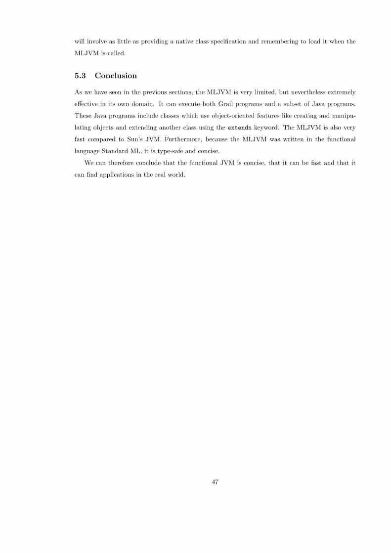
will involve as little as providing a native class specification and remembering to load it when the
MLJVM is called.
5.3 Conclusion
As we have seen in the previous sections, the MLJVM is very limited, but nevertheless extremely
effective in its own domain. It can execute both Grail programs and a subset of Java programs.
These Java programs include classes which use object-oriented features like creating and manipu-
lating objects and extending another class using the extends keyword. The MLJVM is also very
fast compared to Sun’s JVM. Furthermore, because the MLJVM was written in the functional
language Standard ML, it is type-safe and concise.
We can therefore conclude that the functional JVM is concise, that it can be fast and that it
can find applications in the real world.
47

References
[Ben98] N. Benton, A. Kennedy and G. Russell, Compiling Standard ML to Java Bytecodes,
In Proceedings of the 3rd ACM SIGPLAN Conference on Functional Programming,
Baltimore. ACM Press, September 1998.
[Ben99] N. Benton and A. Kennedy, Interlanguage Working Without Tears: Blending SML
with Java, In Proceedings of the 4th ACM SIGPLAN Conference on Functional Pro-
gramming, Paris. ACM Press, September 1999.
[MLj99] N. Benton, A. Kennedy, G. Russell, MLj User Guide,
http://www.dcs.ed.ac.uk/home/mlj/doc/index.html,
Cambridge 1999.
[Ber98] Peter Bertelsen, Compiling SML to Java Bytecode,
http://www.dina.dk/~pmb/publications.html,
Master’s Thesis, Department of Information Technology, Technical University of Den-
mark, January 1998.
[Lea03] C. League, Z. Shao and V. Trifonov, Precision in Practice: A Type-Preserving Java
Compiler, In Proc. 12th International Conference on Compiler Construction (CC’03),
Warsaw, Poland, April 2003. Lecture Notes in Computer Science Vol. 2622. Springer-
Verlag.
[Lin99] Tim Lindholm & Frank Yellin, The Java�
Virual Machine Specification, Second Edi-
tion ,
http://java.sun.com/docs/books/vmspec/,
Addison-Wesley 1999.
[Mac02] Kenneth MacKenzie, A Virtual Machine Platform for Resource-Bounded Computa-
tion,
http://www.dcs.ed.ac.uk/home/mrg/publications/,
MRG 2002.
[Mey97] Jon Meyer & Troy Downing, Java Virtual Machine, O’Reilly 1997.
[Mey98w] Jon Meyer, Jasmin Home Page,
http://mrl.nyu.edu/~meyer/jasmin/,
GNU 1998.
[MRG] Mobile Resource Guarantees, MRG Home Page,
http://www.dcs.ed.ac.uk/home/mrg/publications/,
Edinburgh University 2003.
48

[Pau96] L.C. Paulson, ML for the Working Programmer, Second Edition, Cambridge Univer-
sity Press 1996.
[Ven00] Bill Venners, Inside the Java Virtual Machine, Second Edition, McGraw-Hill 2000.
49

A MLJVM Mini Manual
Both the MLJVM source files and this thesis can be downloaded from:
http://homepages.inf.ed.ac.uk/stg/research/projects/MLJVM/
Once downloaded, extract the files to some directory, specify the MLJVM home directory in
CompileAll.sml and run the file once. For example:
Shell> mosml CompileAll.sml
If the compilation is successful, one can start can using the main functions immediately. For
example:
Mosml> JasminPrint.pretty_print (Parser.parse "MyClassFile.class");
Mosml> Execute.bootload "MyClassFile.class" ["arg1","arg2"];
After the program CompileAll.sml has completed compiling the MLJVM, it creates a file MLJVM.sml
which can be used for future MLJVM sessions:
Shell> mosml MLJVM.sml
50
B Grail Examples
Ian Stark wrote the three Grail example programs printed below. They are available for download-
ing from [MRG]
B.1 HelloWorld.gr
//
// Time-stamp: <Saturday 26 April 2003 / HelloWorld.gr>
//
// Complete Grail program to print "Hello, World."
//
// Ian Stark
class HelloWorld {
method public static void main (java.lang.String[] args) =
let
val o = getstatic <java.io.PrintStream java.lang.System.out>
in
invokevirtual o
<void java.io.PrintStream.println(java.lang.String)> ("Hello, World.")
end
}
// End of file
51
B.2 Fib.gr
//
// Time-stamp: <Wednesday 5 March 2003 / Fib.gr>
//
// Calculate the n’th Fibonacci number in linear time
//
// This is a complete program; compile and run thus:
//
// $ gdf Fib.gr
// Compiled Fib.gr
// $ java Fib 2 3 0
// fib(2) = 1
// fib(3) = 2
// fib(0) = 1
// $
//
// Ian Stark
class Fib {
// Calculate the Fibonacci number, tracking two at once for speed
method static int fib (int n) =
let val a = 0
val b = 1
fun loop (int a, int b, int n) =
let val b = add a b
val a = sub b a
val n = sub n 1
in
test(a,b,n)
end
fun test (int a, int b, int n) =
if n<=1 then b else loop(a,b,n)
in
test(a,b,n)
end
// Main method; scan arguments, convert to integers, act on each
method public static void main (java.lang.String[] args) =
let
val j = 0
val n = 0
fun test (java.lang.String[] args, int j) =
let val l = length args
in
if j >= l then () else print(args,j)
end
fun print (java.lang.String[] args, int j) =
let
val s = get args j
val n = invokestatic
<int java.lang.Integer.parseInt(java.lang.String)> (s)
val m = invokestatic <int Fib.fib(int)> (n)
val () = invokestatic <void Fib.print(int,int)> (n,m)
val j = add j 1
in
52

test(args,j)
end
in
test(args,j)
end
// Output method; take two integers and print a message about them
method public static void print (int n, int m) =
let
val o = getstatic <java.io.PrintStream java.lang.System.out>
val () = invokevirtual o
<void java.io.PrintStream.print(java.lang.String)> ("fib(")
val () = invokevirtual o <void java.io.PrintStream.print(int)> (n)
val () = invokevirtual o
<void java.io.PrintStream.print(java.lang.String)> (") = ")
in
invokevirtual o <void java.io.PrintStream.println(int)> (m)
end
}
// End of file
53

B.3 SumList.gr
// Find the sum of a list of integers given on the command line
// Mostly to demonstrate how to write a standalone program in Grail
class SumList
{
method public static void main (java.lang.String[] args) =
let
val acc = 0
val index = 0
val num_args = length args
fun print_sum (java.lang.String[] args, int index, int acc, int num_args) =
if index >= num_args then print_acc (acc)
else print_sum’ (args, index, acc, num_args)
fun print_sum’(java.lang.String[] args, int index, int acc, int num_args) =
let
val entry = get args index
val numeric_entry =
invokestatic <int java.lang.Integer.parseInt(java.lang.String)> (entry)
val acc = add acc numeric_entry
val index = add index 1
in
print_sum (args, index, acc, num_args)
end
fun print_acc(int acc) =
let
val out = getstatic <java.io.PrintStream java.lang.System.out>
in
invokevirtual out <void java.io.PrintStream.println(int)> (acc)
end
in
print_sum (args, index, acc, num_args)
end
}
54
C Java Examples
C.1 Q1.java, Q2.java and Q3.java
public class Q1 {
public static int counter = 0;
public static void qprint(String s) {
System.out.print("Static method *qprint* called by: *");
System.out.print(s);
System.out.println("*");
}
public void qprinti(String s) {
System.out.print("Instance method *qprinti* called by: *");
System.out.print(s);
System.out.println("*");
}
}
public class Q2 extends Q1 {
public static void main(String[] args) {
qprint("Q2.main");
Q2 q2 = new Q2();
q2.qprinti("Q2.main");
System.out.println(counter);
}
}
public class Q3 extends Q2 {
public static void main(String[] args) {
qprint("Q3.main");
Q3 q3 = new Q3();
q3.qprinti("Q3.main");
System.out.println(counter);
}
}
55
C.2 ExOne.java
public class ExOne {
public static void main(String[] args) {
int j = 0;
while (j < 10) {
System.out.print("Looping with j@");
System.out.println(j);
j++;
}
for (int i=0;i<20;i++) {
System.out.print("Looping with i@");
System.out.println(i);
}
}
}
56
C.3 ExTwo.java
public class ExTwo {
static int counter = 0;
int i1;
int i2;
public ExTwo() {
i1 = 10;
i2 = 10 + counter;
counter = counter + 1;
}
public static int my_add(ExTwo e) {
int z = e.i1 + e.i2;
return z;
}
public static void main(String[] args) {
ExTwo e1 = new ExTwo();
int answer1 = my_add(e1);
System.out.println(answer1);
ExTwo e2 = new ExTwo();
int answer2 = my_add(e2);
System.out.println(answer2);
ExTwo e3 = new ExTwo();
int answer3 = my_add(e3);
System.out.println(answer3);
}
}
57
C.4 ExThree.java
public class ExThree {
public static void main(String[] args) {
int answer = Integer.parseInt(args[0]) + 10;
System.out.print(args[0]);
System.out.print(" + 10 = ");
System.out.println(answer);
}
}
58

![MachineLearningforBrainImagesClassificationofTwo ...2019/12/21 · pletely solved [1, 2]. Several machine learning (ML) tech-niques have been implemented to classify brain activity,](https://img.pdfslide.net/doc/110x75/611c8b8d96b21e73423566f3/machinelearningforbrainimagesclassificationoftwo-20191221-pletely-solved.jpg)


![Home [ddi.cs.uni-potsdam.de]ddi.cs.uni-potsdam.de/HyFISCH/Produzieren/MultimediaA… · Web viewProgramming interface that allows to add custom question types implemented in Java,](https://img.pdfslide.net/doc/110x75/5f24c05e17231e01e64d94b6/home-ddicsuni-ddicsuni-web-view-programming-interface-that-allows-to-add.jpg)