BNL-113457-2017-JA File # 94411

Modal phase measuring deflectometry

Lei Huang, Junpeng Xue, Bo Gao,

Chris McPherson, Jacob Beverage, and Mourag Idir

Submitted to Optics Express

October 17, 2016

Photon Sciences Department

Brookhaven National Laboratory

U.S. Department of EnergyUSDOE Office of Science (SC),

Basic Energy Sciences (BES) (SC-22)

Notice: This manuscript has been authored by employees of Brookhaven Science Associates, LLC under Contract No. DE- SC0012704 with the U.S. Department of Energy. The publisher by accepting the manuscript for publication acknowledges that the United States Government retains a non-exclusive, paid-up, irrevocable, world-wide license to publish or reproduce the published form of this manuscript, or allow others to do so, for United States Government purposes.

DISCLAIMER

This report was prepared as an account of work sponsored by an agency of the United States Government. Neither the United States Government nor any agency thereof, nor any of their employees, nor any of their contractors, subcontractors, or their employees, makes any warranty, express or implied, or assumes any legal liability or responsibility for the accuracy, completeness, or any third party’s use or the results of such use of any information, apparatus, product, or process disclosed, or represents that its use would not infringe privately owned rights. Reference herein to any specific commercial product, process, or service by trade name, trademark, manufacturer, or otherwise, does not necessarily constitute or imply its endorsement, recommendation, or favoring by the United States Government or any agency thereof or its contractors or subcontractors. The views and opinions of authors expressed herein do not necessarily state or reflect those of the United States Government or any agency thereof.

1 

Modal Phase Measuring Deflectometry 1 

LEI HUANG,1,* JUNPENG XUE,1,2 BO GAO,1,3,4 CHRIS MCPHERSON,5 JACOB2 

BEVERAGE,5 AND MOURAD IDIR13 

1Brookhaven National Laboratory - NSLS II, 50 Rutherford Dr. Upton, NY 11973-5000, USA 4 2School of Aeronautics and Astronautics, Sichuan University, Chengdu 610065, China 5 3Shanghai Institute of Applied Physics, Chinese Academy of Sciences, Shanghai 201800, China 6 4University of Chinese Academy of Sciences, Beijing 100049, China 7 5Arizona Optical Systems, Tucson, AZ 85747, USA 8 *huanglei0114@gmail.com 9 

Abstract: In this work, a model based method is applied to phase measuring deflectometry, 10 which is named as modal phase measuring deflectometry. The height and slopes of the 11 surface under test are represented by mathematical models and updated by optimizing the 12 model coefficients to minimize the discrepancy between the reprojection in ray tracing and 13 the actual measurement. The pose of the screen relative to the camera is pre-calibrated and 14 further optimized together with the shape coefficients of the surface under test. Simulations 15 and experiments are conducted to demonstrate the feasibility of the proposed approach. 16 © 2016 Optical Society of America 17 OCIS Codes: (120.0120) Instrumentation, measurement, and metrology; (120.5050) Phase measurement; (120.3940) 18 Metrology.19 

References and Links 20 

1. P. de Groot, "Principles of interference microscopy for the measurement of surface topography," Advances in 21 Optics and Photonics 7, 1-65 (2015). 22 

2. F. Chen, G. M. Brown, and M. Song, "Overview of three-dimensional shape measurement using optical 23 methods," Optical Engineering 39, 10-22 (2000). 24 

3. M. C. Knauer, J. Kaminski, and G. Häusler, "Phase measuring deflectometry: a new approach to measure 25 specular free-form surfaces," in Optical Metrology in Production Engineering, Proc. SPIE (SPIE, 2004), 366-26 376. 27 

4. M. Petz and R. Tutsch, "Reflection grating photogrammetry: a technique for absolute shape measurement of 28 specular free-form surfaces," in Optical Manufacturing and Testing VI, Proc. SPIE (SPIE 2005), 29 58691D58691-58691D58612. 30 

5. T. Bothe, W. Li, C. von Kopylow, and W. P. O. Jüptner, "High-resolution 3D shape measurement on specular 31 surfaces by fringe reflection," in Optical Metrology in Production Engineering, Proc. SPIE (SPIE, 2004), 411-32 422. 33 

6. C. Faber, E. Olesch, R. Krobot, and G. Häusler, "Deflectometry challenges interferometry: the competition gets 34 tougher!," in 2012), 84930R-84930R-84915. 35 

7. Y. Tang, X. Su, Y. Liu, and H. Jing, "3D shape measurement of the aspheric mirror by advanced phase 36 measuring deflectometry," Opt. Express 16, 15090-15096 (2008). 37 

8. L. Huang, C. S. Ng, and A. K. Asundi, "Dynamic three-dimensional sensing for specular surface with 38 monoscopic fringe reflectometry," Opt. Express 19, 12809-12814 (2011). 39 

9. Y. Liu, E. Olesch, Z. Yang, and G. Häusler, "Fast and accurate deflectometry with crossed fringes," Advanced 40 Optical Technologies 3, 441-445 (2014). 41 

10. P. Su, R. E. Parks, L. Wang, R. P. Angel, and J. H. Burge, "Software configurable optical test system: a42 computerized reverse Hartmann test," Applied Optics 49, 4404-4412 (2010). 43 

11. P. Su, Y. Wang, J. H. Burge, K. Kaznatcheev, and M. Idir, "Non-null full field X-ray mirror metrology using 44 SCOTS: a reflection deflectometry approach," Optics Express 20, 12393-12406 (2012). 45 

12. R. Huang, P. Su, J. H. Burge, and M. Idir, "X-ray mirror metrology using SCOTS/deflectometry," in 2013), 46 88480G-88480G-88486. 47 

13. H. Yue, Y. Wu, B. Zhao, Z. Ou, Y. Liu, and Y. Liu, "A carrier removal method in phase measuring48 deflectometry based on the analytical carrier phase description," Optics Express 21, 21756-21765 (2013). 49 

14. T. Su, A. Maldonado, P. Su, and J. H. Burge, "Instrument transfer function of slope measuring deflectometry 50 systems," Applied Optics 54, 2981-2990 (2015). 51 

15. D. Sprenger, C. Faber, M. Seraphim, and G. Häusler, "UV-Deflectometry: No parasitic reflections," in Proc. 52 DGaO, 2010), A19. 53 

2  

16. L. Huang, M. Idir, C. Zuo, K. Kaznatcheev, L. Zhou, and A. Asundi, "Comparison of two-dimensional 54 integration methods for shape reconstruction from gradient data," Optics and Lasers in Engineering 64, 1-11 55 (2015). 56 

17. S. Ettl, J. Kaminski, M. C. Knauer, and G. Häusler, "Shape reconstruction from gradient data," Appl. Opt. 47, 57 2091-2097 (2008). 58 

18. L. Huang, C. S. Ng, and A. K. Asundi, "Fast full-field out-of-plane deformation measurement using fringe 59 reflectometry," Optics and Lasers in Engineering 50, 529-533 (2012). 60 

19. W. Li, M. Sandner, A. Gesierich, and J. Burke, "Absolute optical surface measurement with deflectometry," in 61 2012), 84940G-84940G-84947. 62 

20. E. Olesch, C. Faber, and G. Häusler, "Deflectometric Self-Calibration for arbitrary specular surfaces," in Proc. 63 112th Annual Meeting of the DGaO A. Vol. 3., (DGaO 2011), 64 

21. L. Miaomiao, R. Hartley, and M. Salzmann, "Mirror Surface Reconstruction from a Single Image," Pattern 65 Analysis and Machine Intelligence, IEEE Transactions on 37, 760-773 (2015). 66 

22. L. Miaomiao, R. Hartley, and M. Salzmann, "Mirror Surface Reconstruction from a Single Image," in 67 Computer Vision and Pattern Recognition (CVPR), 2013 IEEE Conference on, 2013), 129-136. 68 

23. Y.-L. Xiao, X. Su, and W. Chen, "Flexible geometrical calibration for fringe-reflection 3D measurement," Opt. 69 Lett. 37, 620-622 (2012). 70 

24. H. Ren, F. Gao, and X. Jiang, "Iterative optimization calibration method for stereo deflectometry," Optics 71 Express 23, 22060-22068 (2015). 72 

25. R. Huang, P. Su, J. H. Burge, L. Huang, and M. Idir, "High-accuracy aspheric x-ray mirror metrology using 73 Software Configurable Optical Test System/deflectometry," Optical Engineering 54, 084103-084103 (2015). 74 

26. I. Mochi and K. A. Goldberg, "Modal wavefront reconstruction from its gradient," Applied Optics 54, 3780-75 3785 (2015). 76 

27. F. Dai, F. Tang, X. Wang, O. Sasaki, and P. Feng, "Modal wavefront reconstruction based on Zernike 77 polynomials for lateral shearing interferometry: comparisons of existing algorithms," Applied Optics 51, 5028-78 5037 (2012). 79 

28. G.-m. Dai, "Modal wave-front reconstruction with Zernike polynomials and Karhunen-Loève functions," 80 Journal of the Optical Society of America A 13, 1218-1225 (1996). 81 

29. P. C. L. Stephenson, "Recurrence relations for the Cartesian derivatives of the Zernike polynomials," Journal of 82 the Optical Society of America A 31, 708-715 (2014). 83 

30. F. Brunet, "Contributions to parametric image registration and 3d surface reconstruction," European Ph. D. in 84 Computer Vision, Université dAuvergne, Clérmont-Ferrand, France, and Technische Universitat Munchen, 85 Germany (2010). 86 

31. J. Tian, X. Peng, and X. Zhao, "A generalized temporal phase unwrapping algorithm for three-dimensional 87 profilometry," Optics and Lasers in Engineering 46, 336-342 (2008). 88 

32. L. Huang and A. K. Asundi, "Phase invalidity identification framework with the temporal phase unwrapping 89 method," Measurement Science and Technology 22, 035304 (2011). 90 

33. C. Zuo, L. Huang, M. Zhang, Q. Chen, and A. Asundi, "Temporal phase unwrapping algorithms for fringe 91 projection profilometry: A comparative review," Optics and Lasers in Engineering 85, 84-103 (2016). 92 

1. Introduction 93 

Three-dimensional (3D) shape information is always placed at the top of the wish list while 94 an object is under investigation. Extensive studies have been conducted to measure 3D shapes 95 of different surfaces in multiple scales [1, 2]. Similar to interferometry, phase measuring 96 deflectometry (PMD) was proposed primarily for specular surfaces [3-5], but different from 97 interferometry, PMD is an incoherent method with a capability of providing full-field 98 topography data for free-form surfaces [6]. During years after its proposal, progress in several 99 aspects has been made: Tang et al. utilized the PMD technique for aspherical mirror 100 measurement [7]. Dynamic 3D shape measurement has been demonstrated with the fringe 101 reflection technique [8]. Liu el al. use cross fringe patterns to implement fast and accurate 102 PMD [9]. Su et al. carried out series of work with their SCOTS on mirror measurement 103 including telescope mirrors and x-ray mirrors [10-12]. Yue et al. addressed the carrier 104 removal in PMD with analytical description [13]. Not limited in visible light, deflectometry 105 has been pushed into fields of infrared [14] and ultraviolet [15]. Via comparison with 106 interferometry, Faber et al. demonstrated PMD is heading towards being a serious competitor 107 for interferometry [6]. 108 

However, as a slope metrology tool, there is an inherent ambiguity in deflectometry about 109 the calculation for the height and slopes of the surface under test (SUT). Classically the 110 surface height is reconstructed from slopes through integration [16, 17], while the slopes are 111 determined with height knowledge in prior. Due to the uncertainty of the prior knowledge on 112 

3  

height, the introduced slope error will propagate into the resultant height via an integration 113 process. The height-slope ambiguity issue was traditionally ignored or partially solved by 114 roughly assuming a prior height distribution [18], a height-known seeding point [19], iterative 115 reconstruction [20], or stereo vision [3]. Recently, Liu et al. proposed several ways to 116 reconstruct the specular surface shape from a single image with no ambiguity [21, 22]. 117 Another issue we will discuss is the system calibration, which is an everlasting topic in 118 metrology. The classical PMD calibration method can be split into three separate steps for the 119 calibration of screen, cameras, and the system geometry [3, 4]. A flexible way to calibrate the 120 PMD system with a markerless flat mirror was proposed by Xiao et al. [23] and a similar idea 121 has been applied to calibrate stereoscopic PMD system by Ren et al. [24]. Laser tracker was. 122 employed to measure the system geometry [12, 25]. In this work, we present a method to 123 simultaneously estimate the height and slopes of the SUT in PMD by using mathematical 124 models (e.g. Chebyshev polynomials, Zernike polynomials, or B-splines), which is called 125 modal phase measuring deflectometry (MPMD). Moreover, a post-optimization for the screen 126 geometry after the pre-calibration of the PMD system is also addressed in MPMD. 127 

Section 2 introduces the principle of the proposed MPMD with its post-optimization. 128 Simulations for both monoscopic PMD (mono-PMD) and stereoscopic PMD (stereo-PMD) 129 configurations are carried out in section 3 to demonstrate the performance of MPMD. The 130 feasibility of the proposed method is verified with experiments in section 4. Some features in 131 using the proposed MPMD are discussed in section 5, and section 6 concludes the work. 132 

2. Principle 133 

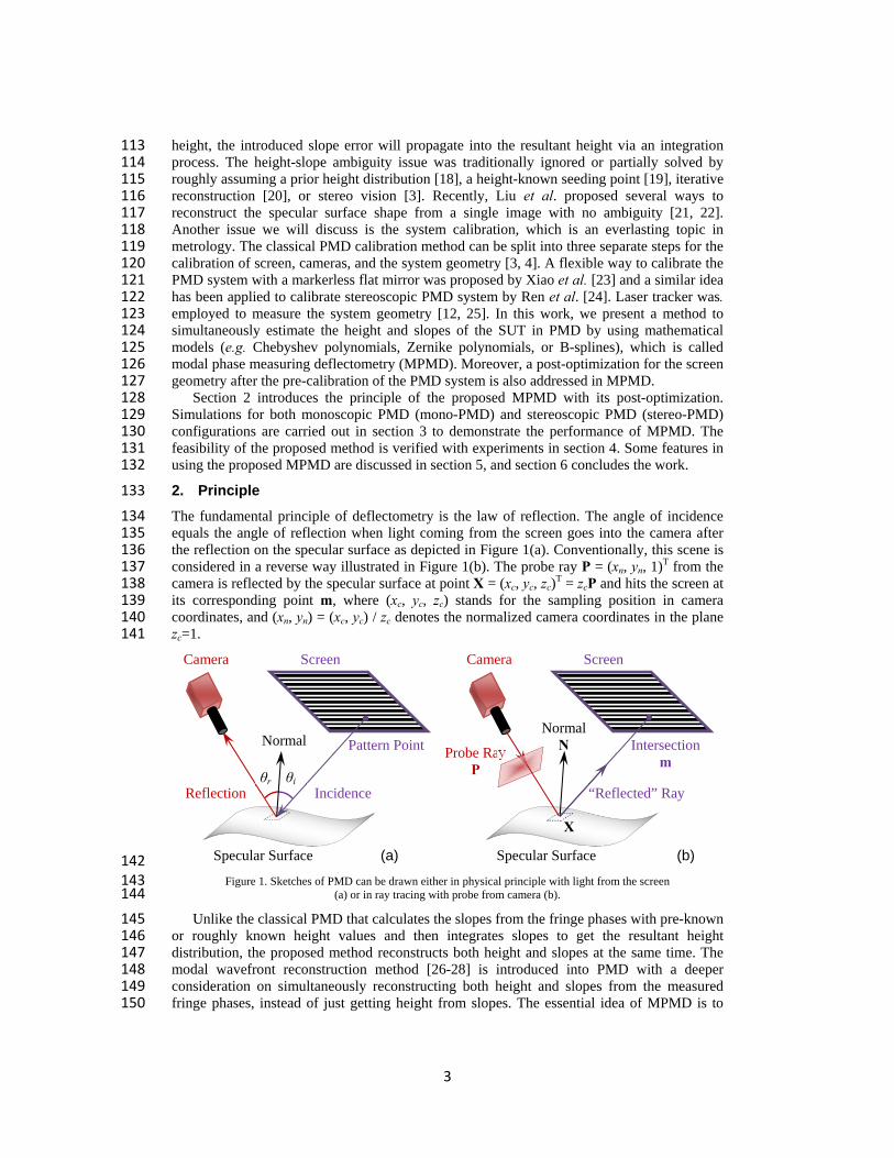
The fundamental principle of deflectometry is the law of reflection. The angle of incidence 134 equals the angle of reflection when light coming from the screen goes into the camera after 135 the reflection on the specular surface as depicted in Figure 1(a). Conventionally, this scene is 136 considered in a reverse way illustrated in Figure 1(b). The probe ray P = (xn, yn, 1)T from the 137 camera is reflected by the specular surface at point X = (xc, yc, zc)T = zcP and hits the screen at 138 its corresponding point m, where (xc, yc, zc) stands for the sampling position in camera 139 coordinates, and (xn, yn) = (xc, yc) / zc denotes the normalized camera coordinates in the plane 140 zc=1. 141 

142 Figure 1. Sketches of PMD can be drawn either in physical principle with light from the screen 143 

(a) or in ray tracing with probe from camera (b). 144 

Unlike the classical PMD that calculates the slopes from the fringe phases with pre-known 145 or roughly known height values and then integrates slopes to get the resultant height 146 distribution, the proposed method reconstructs both height and slopes at the same time. The 147 modal wavefront reconstruction method [26-28] is introduced into PMD with a deeper 148 consideration on simultaneously reconstructing both height and slopes from the measured 149 fringe phases, instead of just getting height from slopes. The essential idea of MPMD is to 150 

Camera Screen

Reflection Incidence

Normal

Specular Surface

θr θi

Pattern Point

(a)

Probe Ray P

Camera Screen

“Reflected” Ray

NormalN

Specular Surface

Intersection m

(b)

X

4  

represent both height and slopes of the SUT with well-established mathematical models w 151 and to optimize the coefficient vector c to best explain the captured fringe patterns in 152 measurement. In order to avoid recalculating basis function during iterations in optimization, 153 which could be time consuming, the shape models are defined in the normalized camera 154 coordinates (xn, yn). 155 

cz w c , (1) 156 

cx

n

z

x

w c , (2) 157 

cy

n

z

y

w c , (3) 158 

where w is the vector of the known basis functions, which can be Chebyshev polynomials, 159 Zernike polynomials, or B-splines. Vectors wx and wy are the known derivatives derived from 160 the corresponding basis function [29, 30]. The unknown vector c contains the coefficients to 161 be optimized for each mode. The length of c is determined by the number of terms in 162 Chebyshev and Zernike polynomials, or the number of control points in B-splines. 163 

Considering the following relations 164 

c c c c c c c c cc n n

n c n c n c n c n

c c c c c c c c cn c n

n c n c n c n c n

z z x z y z z z zz x y

x x x y x x x y x

z z x z y z z z zx z y

y x y y y x y y y

. (4) 165 

The x- and y-slopes in camera coordinates (xc, yc) are represented as 166 

c

c n

c ccc n n

n n

z

z xz zx z x yx y

, (5) 167 

c

c n

c ccc n n

n n

z

z yz zy z x yx y

. (6) 168 

Therefore, the normal of the mirror surface facing towards the camera is 169 

, , 1c c

c c

z z

x y

N . For a probe vector P, its sampling point on the SUT is X and 170 

the vector of the reflected ray from X can be calculated as 171 

2 , r p p n n , (7) 172 

5  

where N

nN

is the normalized normal and P

pP

is the normalized probe vector. 173 

The reflected ray can be determined once its direction (r) and one point on it (X) are 174 

known. If we want to calculate the corresponding intersection m̂ on the screen, it is required 175 to have the pose of the screen relative to the camera (3x1 rotation vector ω, 3x1 translation 176 vector T), which can be obtained through a pre-calibration procedure. The same as the 177 classical calibration [3, 4], the pre-calibration includes the camera calibration, screen 178 calibration, and geometric calibration. Once the pose of the screen is initialized via pre-179 

calibration, the intersection m̂ can be calculated by solving equations of the screen plane 180 and reflected ray. Another purpose of pre-calibration is to initialize coefficient vector c by 181 fitting a camera calibration plane close to where the SUT is going to place. 182 

The coefficient vector c and the pose of the screen (ω, T) in camera coordinates are 183 

optimized by minimizing the differences between the reprojection m̂ and the measurement 184 m on the screen among the N pairs of correspondence in a least squares sense. This 185 nonlinear least squares problem in Eq. (8) can be solved by the Levenberg-Marquardt 186 algorithm. 187 

2

, , 1

ˆˆ ˆ ˆ, , arg min , ,N

n nn

ω T c

ω T c m ω T c m . (8) 188 

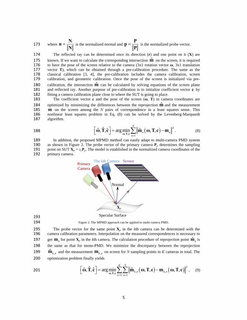
In addition, the proposed MPMD method can easily adapt to multi-camera PMD system 189 as shown in Figure 2. The probe vector of the primary camera Pp determines the sampling 190 point on SUT Xp = zcPp. The model is established in the normalized camera coordinates of the 191 primary camera. 192 

193 Figure 2. The MPMD approach can be applied to multi-camera PMD. 194 

The probe vector for the same point Xp in the kth camera can be determined with the 195 camera calibration parameters. Interpolation on the measured correspondences is necessary to 196 

get km for point Xp in the kth camera. The calculation procedure of reprojection point ˆkm is 197 

the same as that for mono-PMD. We minimize the discrepancy between the reprojection 198 

,ˆ k nm and the measurement ,k nm on screen for N sampling points in K cameras in total. The 199 

optimization problem finally yields 200 

2, ,, , 1 1

ˆˆ ˆ ˆ, , arg min , , , ,K N

k n k nk n

ω T c

ω T c m ω T c m ω T c , (9) 201 

Screen

Normal

Specular Surface

Xp

The kth CameraPrimary Camera

6  

where ,k nm is also a function of parameters (ω, T, c) except the primary camera which 202 

always keeps the same probe ray with no interpolation process. The problem in Eq. (9) can be 203 solved by a nonlinear least squares solver. 204 

3. Simulation 205 

Series of simulations for both mono-PMD and stereo-PMD system are conducted to 206 demonstrate the feasibility of the proposed MPMD approach. In this section, the system 207 configuration in our simulation is described at first, and then the evaluation of the measured 208 shape error is discussed. After the reconstruction under perfect system calibration is 209 addressed, the reconstruction under imperfect pre-calibration will be demonstrated to show 210 the effectiveness of the post-optimization. 211 

System configurations 212 

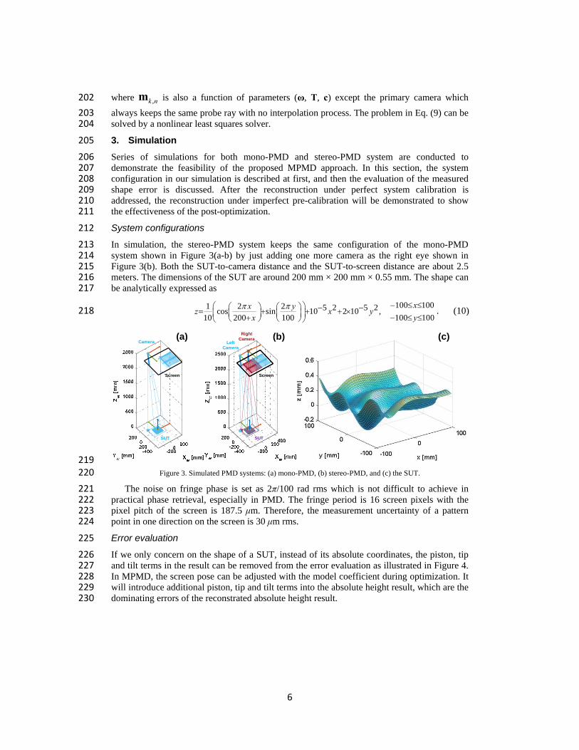
In simulation, the stereo-PMD system keeps the same configuration of the mono-PMD 213 system shown in Figure 3(a-b) by just adding one more camera as the right eye shown in 214 Figure 3(b). Both the SUT-to-camera distance and the SUT-to-screen distance are about 2.5 215 meters. The dimensions of the SUT are around 200 mm × 200 mm × 0.55 mm. The shape can 216 be analytically expressed as 217 

100 1001 2 2 5 5cos sin 10 2 10 , 100 10010 200 10

20

2 xx yz y

xx

y

. (10) 218 

219 Figure 3. Simulated PMD systems: (a) mono-PMD, (b) stereo-PMD, and (c) the SUT. 220 

The noise on fringe phase is set as 2π/100 rad rms which is not difficult to achieve in 221 practical phase retrieval, especially in PMD. The fringe period is 16 screen pixels with the 222 pixel pitch of the screen is 187.5 μm. Therefore, the measurement uncertainty of a pattern 223 point in one direction on the screen is 30 μm rms. 224 

Error evaluation 225 

If we only concern on the shape of a SUT, instead of its absolute coordinates, the piston, tip 226 and tilt terms in the result can be removed from the error evaluation as illustrated in Figure 4. 227 In MPMD, the screen pose can be adjusted with the model coefficient during optimization. It 228 will introduce additional piston, tip and tilt terms into the absolute height result, which are the 229 dominating errors of the reconstrated absolute height result. 230 

Camera

Screen

SUT

LeftCamera

RightCamera

Screen

SUT

(c) (a) (b)

7  

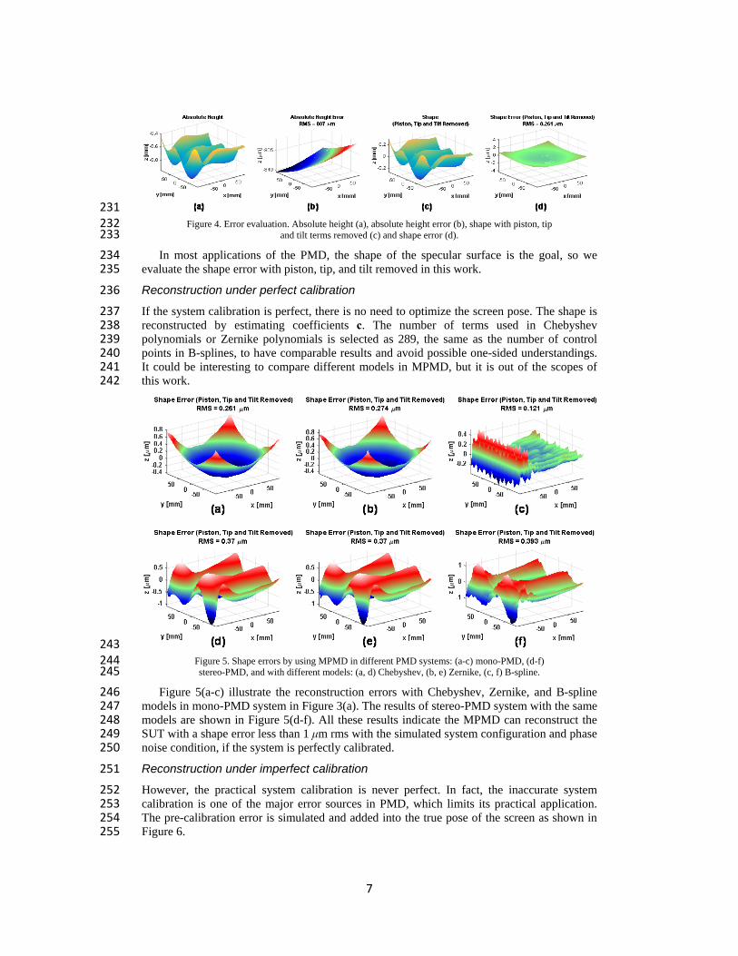
231 Figure 4. Error evaluation. Absolute height (a), absolute height error (b), shape with piston, tip 232 

and tilt terms removed (c) and shape error (d). 233 

In most applications of the PMD, the shape of the specular surface is the goal, so we 234 evaluate the shape error with piston, tip, and tilt removed in this work. 235 

Reconstruction under perfect calibration 236 

If the system calibration is perfect, there is no need to optimize the screen pose. The shape is 237 reconstructed by estimating coefficients c. The number of terms used in Chebyshev 238 polynomials or Zernike polynomials is selected as 289, the same as the number of control 239 points in B-splines, to have comparable results and avoid possible one-sided understandings. 240 It could be interesting to compare different models in MPMD, but it is out of the scopes of 241 this work. 242 

243 Figure 5. Shape errors by using MPMD in different PMD systems: (a-c) mono-PMD, (d-f) 244 stereo-PMD, and with different models: (a, d) Chebyshev, (b, e) Zernike, (c, f) B-spline. 245 

Figure 5(a-c) illustrate the reconstruction errors with Chebyshev, Zernike, and B-spline 246 models in mono-PMD system in Figure 3(a). The results of stereo-PMD system with the same 247 models are shown in Figure 5(d-f). All these results indicate the MPMD can reconstruct the 248 SUT with a shape error less than 1 μm rms with the simulated system configuration and phase 249 noise condition, if the system is perfectly calibrated. 250 

Reconstruction under imperfect calibration 251 

However, the practical system calibration is never perfect. In fact, the inaccurate system 252 calibration is one of the major error sources in PMD, which limits its practical application. 253 The pre-calibration error is simulated and added into the true pose of the screen as shown in 254 Figure 6. 255 

8  

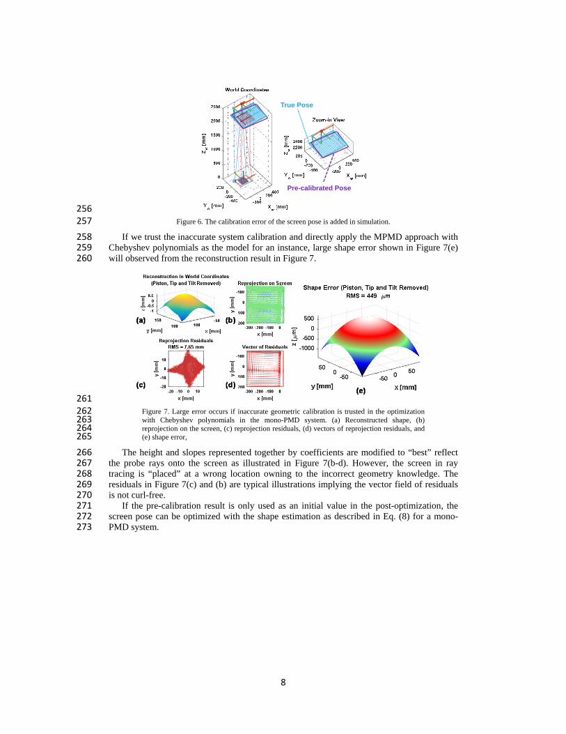
256 Figure 6. The calibration error of the screen pose is added in simulation. 257 

If we trust the inaccurate system calibration and directly apply the MPMD approach with 258 Chebyshev polynomials as the model for an instance, large shape error shown in Figure 7(e) 259 will observed from the reconstruction result in Figure 7. 260 

261 Figure 7. Large error occurs if inaccurate geometric calibration is trusted in the optimization 262 with Chebyshev polynomials in the mono-PMD system. (a) Reconstructed shape, (b) 263 reprojection on the screen, (c) reprojection residuals, (d) vectors of reprojection residuals, and 264 (e) shape error, 265 

The height and slopes represented together by coefficients are modified to “best” reflect 266 the probe rays onto the screen as illustrated in Figure 7(b-d). However, the screen in ray 267 tracing is “placed” at a wrong location owning to the incorrect geometry knowledge. The 268 residuals in Figure 7(c) and (b) are typical illustrations implying the vector field of residuals 269 is not curl-free. 270 

If the pre-calibration result is only used as an initial value in the post-optimization, the 271 screen pose can be optimized with the shape estimation as described in Eq. (8) for a mono-272 PMD system. 273 

True Pose

Pre-calibrated Pose

9  

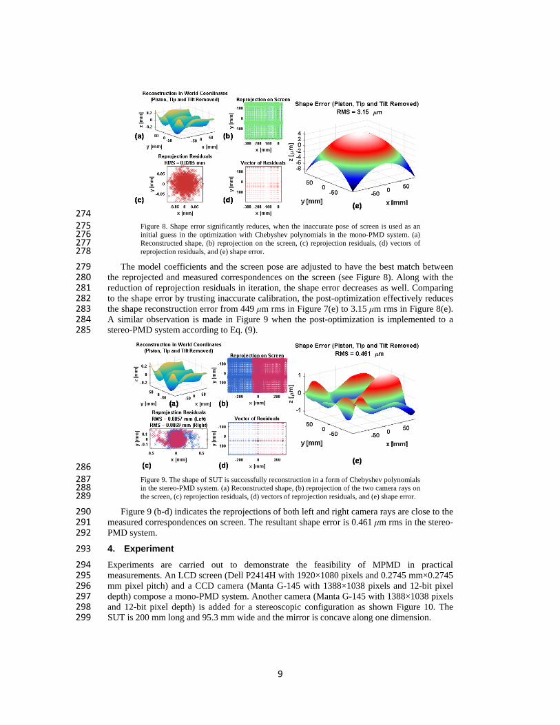
274 Figure 8. Shape error significantly reduces, when the inaccurate pose of screen is used as an 275 initial guess in the optimization with Chebyshev polynomials in the mono-PMD system. (a) 276 Reconstructed shape, (b) reprojection on the screen, (c) reprojection residuals, (d) vectors of 277 reprojection residuals, and (e) shape error. 278 

The model coefficients and the screen pose are adjusted to have the best match between 279 the reprojected and measured correspondences on the screen (see Figure 8). Along with the 280 reduction of reprojection residuals in iteration, the shape error decreases as well. Comparing 281 to the shape error by trusting inaccurate calibration, the post-optimization effectively reduces 282 the shape reconstruction error from 449 μm rms in Figure 7(e) to 3.15 μm rms in Figure 8(e). 283 A similar observation is made in Figure 9 when the post-optimization is implemented to a 284 stereo-PMD system according to Eq. (9). 285 

286 Figure 9. The shape of SUT is successfully reconstruction in a form of Chebyshev polynomials 287 in the stereo-PMD system. (a) Reconstructed shape, (b) reprojection of the two camera rays on 288 the screen, (c) reprojection residuals, (d) vectors of reprojection residuals, and (e) shape error. 289 

Figure 9 (b-d) indicates the reprojections of both left and right camera rays are close to the 290 measured correspondences on screen. The resultant shape error is 0.461 μm rms in the stereo-291 PMD system. 292 

4. Experiment 293 

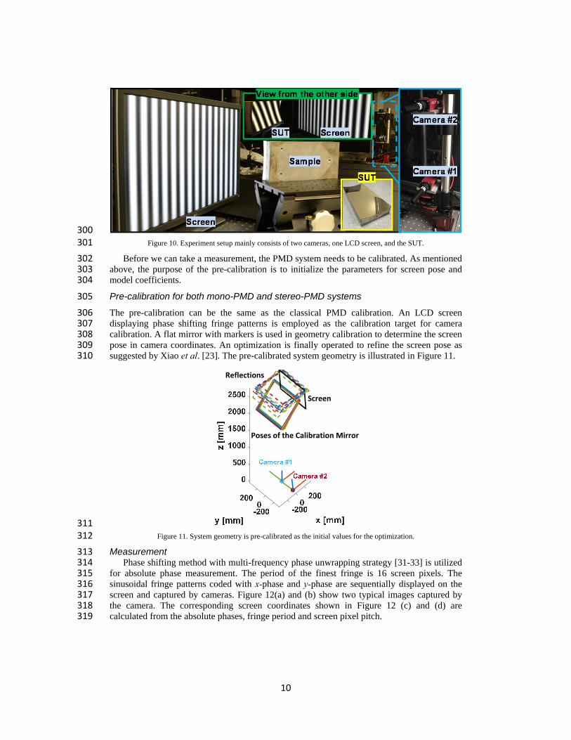
Experiments are carried out to demonstrate the feasibility of MPMD in practical 294 measurements. An LCD screen (Dell P2414H with 1920×1080 pixels and 0.2745 mm×0.2745 295 mm pixel pitch) and a CCD camera (Manta G-145 with 1388×1038 pixels and 12-bit pixel 296 depth) compose a mono-PMD system. Another camera (Manta G-145 with 1388×1038 pixels 297 and 12-bit pixel depth) is added for a stereoscopic configuration as shown Figure 10. The 298 SUT is 200 mm long and 95.3 mm wide and the mirror is concave along one dimension. 299 

10  

300 Figure 10. Experiment setup mainly consists of two cameras, one LCD screen, and the SUT. 301 

Before we can take a measurement, the PMD system needs to be calibrated. As mentioned 302 above, the purpose of the pre-calibration is to initialize the parameters for screen pose and 303 model coefficients. 304 

Pre-calibration for both mono-PMD and stereo-PMD systems 305 

The pre-calibration can be the same as the classical PMD calibration. An LCD screen 306 displaying phase shifting fringe patterns is employed as the calibration target for camera 307 calibration. A flat mirror with markers is used in geometry calibration to determine the screen 308 pose in camera coordinates. An optimization is finally operated to refine the screen pose as 309 suggested by Xiao et al. [23]. The pre-calibrated system geometry is illustrated in Figure 11. 310 

311 Figure 11. System geometry is pre-calibrated as the initial values for the optimization. 312 

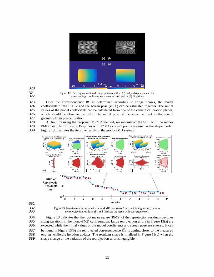
Measurement 313 Phase shifting method with multi-frequency phase unwrapping strategy [31-33] is utilized 314 

for absolute phase measurement. The period of the finest fringe is 16 screen pixels. The 315 sinusoidal fringe patterns coded with x-phase and y-phase are sequentially displayed on the 316 screen and captured by cameras. Figure 12(a) and (b) show two typical images captured by 317 the camera. The corresponding screen coordinates shown in Figure 12 (c) and (d) are 318 calculated from the absolute phases, fringe period and screen pixel pitch. 319 

Screen

Poses of the Calibration Mirror

Reflections

11  

320 Figure 12. Two typical captured fringe patterns with x- (a) and y- (b) phases, and the 321 

corresponding coordinates on screen in x- (c) and y- (d) directions. 322 

Once the correspondence m is determined according to fringe phases, the model 323 coefficients of the SUT c and the screen pose (ω, T) can be estimated together. The initial 324 values of the model coefficients can be calculated from one of the camera calibration planes, 325 which should be close to the SUT. The initial pose of the screen are set as the screen 326 geometry from pre-calibration. 327 

At first, by using the proposed MPMD method, we reconstruct the SUT with the mono-328 PMD data. Uniform cubic B-splines with 17 × 17 control points are used as the shape model. 329 Figure 13 illustrates the iterative results in the mono-PMD system. 330 

331 Figure 13. Iterative optimization with mono-PMD data starts from the initial guess (a), reduces 332 

the reprojection residuals (b), and finalizes the result with convergence (c). 333 

Figure 13 indicates that the root mean square (RMS) of the reprojection residuals declines 334 along iterations in the mono-PMD configuration. Large reprojection errors in Figure 13(a) are 335 expected while the initial values of the model coefficients and screen pose are entered. It can 336 

be found in Figure 13(b) the reprojected correspondence m̂ is getting closer to the measured 337 one m while the iteration updates. The resultant shape is finalized in Figure 13(c) when the 338 shape change or the variation of the reprojection error is negligible. 339 

12  

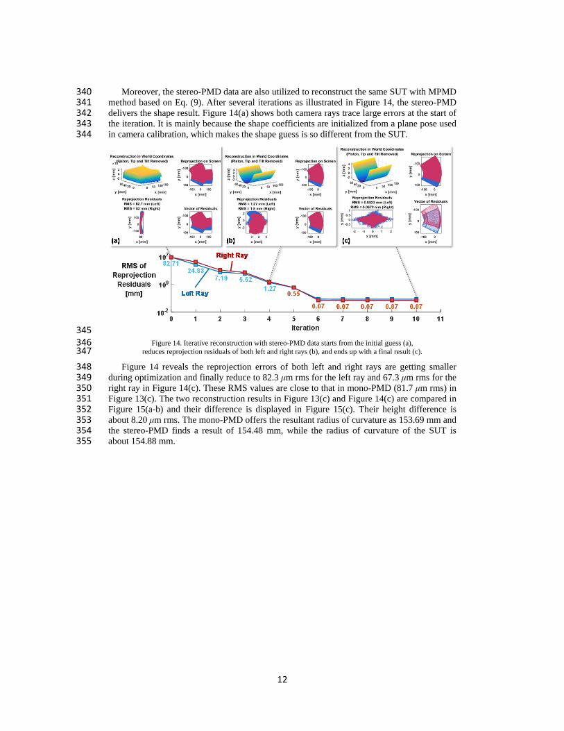
Moreover, the stereo-PMD data are also utilized to reconstruct the same SUT with MPMD 340 method based on Eq. (9). After several iterations as illustrated in Figure 14, the stereo-PMD 341 delivers the shape result. Figure 14(a) shows both camera rays trace large errors at the start of 342 the iteration. It is mainly because the shape coefficients are initialized from a plane pose used 343 in camera calibration, which makes the shape guess is so different from the SUT. 344 

345 Figure 14. Iterative reconstruction with stereo-PMD data starts from the initial guess (a), 346 

reduces reprojection residuals of both left and right rays (b), and ends up with a final result (c). 347 

Figure 14 reveals the reprojection errors of both left and right rays are getting smaller 348 during optimization and finally reduce to 82.3 μm rms for the left ray and 67.3 μm rms for the 349 right ray in Figure 14(c). These RMS values are close to that in mono-PMD (81.7 μm rms) in 350 Figure 13(c). The two reconstruction results in Figure 13(c) and Figure 14(c) are compared in 351 Figure 15(a-b) and their difference is displayed in Figure 15(c). Their height difference is 352 about 8.20 μm rms. The mono-PMD offers the resultant radius of curvature as 153.69 mm and 353 the stereo-PMD finds a result of 154.48 mm, while the radius of curvature of the SUT is 354 about 154.88 mm. 355 

13  

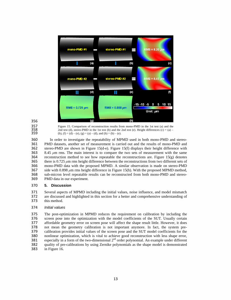
356 Figure 15. Comparison of reconstruction results from mono-PMD in the 1st test (a) and the 357 2nd test (d), stereo-PMD in the 1st test (b) and the 2nd test (e). Height differences (c) = (a) – 358 (b), (f) = (d) – (e), (g) = (a) – (d), and (h) = (b) – (e). 359 

In order to investigate the repeatability of MPMD used in both mono-PMD and stereo-360 PMD datasets, another set of measurement is carried out and the results of mono-PMD and 361 stereo-PMD are shown in Figure 15(d-e). Figure 15(f) displays their height difference with 362 8.45 μm rms. The main interest is to compare the two sets of measurement with the same 363 reconstruction method to see how repeatable the reconstructions are. Figure 15(g) denotes 364 there is 0.725 μm rms height difference between the reconstructions from two different sets of 365 mono-PMD data with the proposed MPMD. A similar observation is made on stereo-PMD 366 side with 0.898 μm rms height difference in Figure 15(h). With the proposed MPMD method, 367 sub-micron level repeatable results can be reconstructed from both mono-PMD and stereo-368 PMD data in our experiment. 369 

5. Discussion 370 

Several aspects of MPMD including the initial values, noise influence, and model mismatch 371 are discussed and highlighted in this section for a better and comprehensive understanding of 372 this method. 373 

Initial values 374 

The post-optimization in MPMD reduces the requirement on calibration by including the 375 screen pose into the optimization with the model coefficients of the SUT. Usually certain 376 affordable geometry error on screen pose will affect the shape result little. However, it does 377 not mean the geometry calibration is not important anymore. In fact, the system pre-378 calibration provides initial values of the screen pose and the SUT model coefficients for the 379 nonlinear optimization, which is vital to achieve good reconstruction with less shape error, 380 especially in a form of the two-dimensional 2nd order polynomial. An example under different 381 quality of pre-calibrations by using Zernike polynomials as the shape model is demonstrated 382 in Figure 16. 383 

14  

384 Figure 16. Pre-calibration is still important although MPMD relaxes the calibration. A good 385 calibration (a) offers better initial values for a better reconstruction with less shape error (b), 386 comparing to a poor calibration (c) with its corresponding large reconstruction error (d) 387 

Figure 16 reveals that MPMD method gets a relatively lower shape error under a good 388 pre-calibration. The reconstruction can be much worse if the pre-calibration is poorly handled 389 with providing an initial guess far from the reality as shown in Figure 16 (c-d). 390 

Noise influence 391 

In classical PMD, the phase noise directly links to the slope noise, so the noise influence 392 occurs at the integration step and depends on the integration algorithm. However, in MPMD, 393 the measurement noise affects the nonlinear optimization and usually it ends up with a global 394 shape error as a result. 395 

Mismatch between the SUT and the model 396 

Another important error source is the mismatch between the SUT and the model with a 397 limited number of polynomial orders or control points. For example, Figure 17(a-d) shows a 398 reconstruction of the SUT by 289 orders of Zernike polynomials. In contrast, if we only use 399 36 orders of Zernike polynomials in reconstruction, the larger reprojection residuals and 400 shape error can be observed in Figure 17(e-h) due to the insufficient Zernike modes to well 401 represent the SUT. 402 

403 Figure 17. Number of model coefficients may influence the reconstruction accuracy. 404 Reprojection residuals (a-b) are smaller and the reconstructed shape (c) is more accurate with 405 less shape error (d) with 289 orders of Zernike polynomials than those (e-h) with 36 orders of 406 Zernike polynomials 407 

15  

The proposed MPMD is not good at reconstructing local waviness on the specular SUT. 408 In some applications, high frequency components are interested and significant. It requires a 409 large number of model coefficients to represent these high frequency terms. However, this 410 will highly increase the computing time and become it impractical. How to better deal with 411 the reprojection residuals and reconstruct the high frequency components in MPMD will be 412 addressed in our future work. 413 

6. Conclusion 414 

Modal phase measuring deflectometry is proposed in this work for mono-PMD, stereo-PMD, 415 and multi-camera PMD configurations. The surface shape is represented by mathematical 416 models (e.g. Chebyshev, Zernike, or B-spline). The model coefficients are adjusted to 417 minimize the reprojection error on the screen. The reconstruction problem becomes a 418 nonlinear optimization problem to match the reprojected correspondences with measured 419 ones. In addition, the screen geometry from calibration is not simply trusted, but used as 420 initial values and optimized with the surface shape optimization. Both simulation and 421 experiment demonstrate the proposed MPMD is effective in 3D shape reconstruction for 422 specular surfaces. 423 

Funding 424 

This work was supported by the US Department of Energy, Office of Science, Office of Basic 425 Energy sciences, under contract No.DE-AC-02-98CH10886. 426 

Acknowledgments 427 

We would like to thank Yuankun Liu in Sichuan University for the extensive discussion on 428 system calibration, Miaomiao Liu in NICTA for the helpful discussion on shape 429 reconstruction, and Dennis Kuhne in the optics and metrology group of NSLS-II for the 430 mechanical machining. 431