Model-Agnostic Counterfactual Reasoning for EliminatingPopularity Bias in Recommender System

Tianxin Wei1, Fuli Feng2∗, Jiawei Chen1, Ziwei Wu1, Jinfeng Yi3 and Xiangnan He1∗1University of Science and Technology of China, 2National University of Singapore, 3JD AI Research

rouseau@mail.ustc.edu.cn,fulifeng93@gmail.com,cjwustc@ustc.edu.cnmaggiewuzw@gmail.com,yijinfeng@jd.com,xiangnanhe@gmail.com

ABSTRACTThe general aim of the recommender system is to provide personal-ized suggestions to users, which is opposed to suggesting popularitems. However, the normal training paradigm, i.e., fitting a recom-mender model to recover the user behavior data with pointwiseor pairwise loss, makes the model biased towards popular items.This results in the terrible Matthew effect, making popular items bemore frequently recommended and become even more popular. Ex-isting work addresses this issue with Inverse Propensity Weighting(IPW), which decreases the impact of popular items on the trainingand increases the impact of long-tail items. Although theoreticallysound, IPW methods are highly sensitive to the weighting strategy,which is notoriously difficult to tune.

In this work, we explore the popularity bias issue from a noveland fundamental perspective — cause-effect. We identify that popu-larity bias lies in the direct effect from the item node to the rankingscore, such that an item’s intrinsic property is the cause of mistak-enly assigning it a higher ranking score. To eliminate popularitybias, it is essential to answer the counterfactual question that whatthe ranking score would be if the model only uses item property. Tothis end, we formulate a causal graph to describe the importantcause-effect relations in the recommendation process. During train-ing, we perform multi-task learning to achieve the contribution ofeach cause; during testing, we perform counterfactual inferenceto remove the effect of item popularity. Remarkably, our solutionamends the learning process of recommendation which is agnos-tic to a wide range of models — it can be easily implemented inexisting methods. We demonstrate it on Matrix Factorization (MF)and LightGCN [20], which are representative of the conventionaland SOTA model for collaborative filtering. Experiments on fivereal-world datasets demonstrate the effectiveness of our method.

CCS CONCEPTS• Information systems→ Recommender systems.

KEYWORDSRecommendation, Popularity Bias, Causal Reasoning

* Fuli Feng and Xiangnan He are Corresponding Authors.

Permission to make digital or hard copies of all or part of this work for personal orclassroom use is granted without fee provided that copies are not made or distributedfor profit or commercial advantage and that copies bear this notice and the full citationon the first page. Copyrights for components of this work owned by others than theauthor(s) must be honored. Abstracting with credit is permitted. To copy otherwise, orrepublish, to post on servers or to redistribute to lists, requires prior specific permissionand/or a fee. Request permissions from permissions@acm.org.KDD ’21, August 14–18, 2021, Virtual Event, Singapore© 2021 Copyright held by the owner/author(s). Publication rights licensed to ACM.ACM ISBN 978-1-4503-8332-5/21/08. . . $15.00https://doi.org/10.1145/3447548.3467289

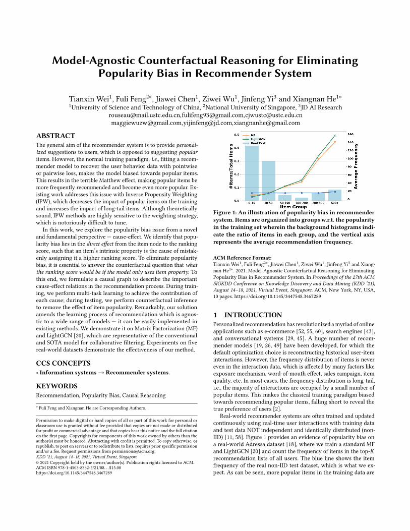
Figure 1: An illustration of popularity bias in recommendersystem. Items are organized into groups w.r.t. the popularityin the training set wherein the background histograms indi-cate the ratio of items in each group, and the vertical axisrepresents the average recommendation frequency.

ACM Reference Format:Tianxin Wei1, Fuli Feng2∗, Jiawei Chen1, Ziwei Wu1, Jinfeng Yi3 and Xiang-nan He1∗. 2021. Model-Agnostic Counterfactual Reasoning for EliminatingPopularity Bias in Recommender System. In Proceedings of the 27th ACMSIGKDD Conference on Knowledge Discovery and Data Mining (KDD ’21),August 14–18, 2021, Virtual Event, Singapore. ACM, New York, NY, USA,10 pages. https://doi.org/10.1145/3447548.3467289

1 INTRODUCTIONPersonalized recommendation has revolutionized amyriad of onlineapplications such as e-commerce [52, 55, 60], search engines [43],and conversational systems [29, 45]. A huge number of recom-mender models [19, 26, 49] have been developed, for which thedefault optimization choice is reconstructing historical user-iteminteractions. However, the frequency distribution of items is nevereven in the interaction data, which is affected by many factors likeexposure mechanism, word-of-mouth effect, sales campaign, itemquality, etc. In most cases, the frequency distribution is long-tail,i.e., the majority of interactions are occupied by a small number ofpopular items. This makes the classical training paradigm biasedtowards recommending popular items, falling short to reveal thetrue preference of users [2].

Real-world recommender systems are often trained and updatedcontinuously using real-time user interactions with training dataand test data NOT independent and identically distributed (non-IID) [11, 58]. Figure 1 provides an evidence of popularity bias ona real-world Adressa dataset [18], where we train a standard MFand LightGCN [20] and count the frequency of items in the top-𝐾recommendation lists of all users. The blue line shows the itemfrequency of the real non-IID test dataset, which is what we ex-pect. As can be seen, more popular items in the training data are

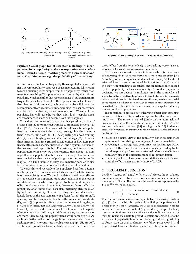
(a) User-item matching (b) Incorporating itempopularity

(c) Incorporating itempopularity and user con-formity

Figure 2: Causal graph for (a) user-item matching; (b) incor-porating item popularity; and (c) incorporating user confor-mity. I: item. U: user. K: matching features between user anditem. Y: ranking score (e.g., the probability of interaction).

recommended much more frequently than expected, demonstrat-ing a severe popularity bias. As a consequence, a model is proneto recommending items simply from their popularity, rather thanuser-item matching. This phenomenon is caused by the trainingparadigm, which identifies that recommending popular items morefrequently can achieve lower loss thus updates parameters towardsthat direction. Unfortunately, such popularity bias will hinder therecommender from accurately understanding the user preferenceand decrease the diversity of recommendations. Worse still, thepopularity bias will cause the Matthew Effect [36] — popular itemsare recommended more and become even more popular.

To address the issues of normal training paradigm, a line ofstudies push the recommender training to emphasize the long-tailitems [7, 31]. The idea is to downweigh the influence from popularitems on recommender training, e.g., re-weighting their interac-tions in the training loss [30, 50], incorporating balanced trainingdata [7] or disentangling user and item embeddings [58]. However,these methods lack fine-grained consideration of how item pop-ularity affects each specific interaction, and a systematic view ofthe mechanism of popularity bias. For instance, the interactions onpopular items will always be downweighted than a long-tail itemregardless of a popular item better matches the preference of theuser. We believe that instead of pushing the recommender to thelong-tail in a blind manner, the key of eliminating popularity biasis to understand how item popularity affects each interaction.

Towards this end, we explore the popularity bias from a funda-mental perspective — cause-effect, which has received little scrutinyin recommender systems. We first formulate a causal graph (Figure2(c)) to describe the important cause-effect relations in the recom-mendation process, which corresponds to the generation processof historical interactions. In our view, three main factors affect theprobability of an interaction: user-item matching, item popular-ity, and user conformity. However, existing recommender modelslargely focus on the user-item matching factor [22, 53] (Figure 2(a)),ignoring how the item popularity affects the interaction probability(Figure 2(b)). Suppose two items have the same matching degreefor a user, the item that has larger popularity is more likely to beknown by the user and thus consumed. Furthermore, such impactsof item popularity could vary for different users, e.g., some usersare more likely to explore popular items while some are not. Assuch, we further add a direct edge from the user node (𝑈 ) to theranking score (𝑌 ) to constitute the final causal graph (Figure 2(c)).To eliminate popularity bias effectively, it is essential to infer the

Figure 3: An example of counterfactual inference.

direct effect from the item node (𝐼 ) to the ranking score (𝑌 ), so asto remove it during recommendation inference.

To this end, we resort to causal inference which is the scienceof analyzing the relationship between a cause and its effect [35].According to the theory of counterfactual inference [35], the directeffect of 𝐼 → 𝑌 can be estimated by imagining a world wherethe user-item matching is discarded, and an interaction is causedby item popularity and user conformity. To conduct popularitydebiasing, we just deduct the ranking score in the counterfactualworld from the overall ranking score. Figure 3 shows a toy examplewhere the training data is biased towards iPhone, making the modelscore higher on iPhone even though the user is more interested inbasketball. Such bias is removed in the inference stage by deductingthe counterfactual prediction.

In our method, to pursue a better learning of user-item matching,we construct two auxiliary tasks to capture the effects of 𝑈 → 𝑌

and 𝐼 → 𝑌 . The model is trained jointly on the main task andtwo auxiliary tasks. Remarkably, our approach is model-agnosticand we implement it on MF [28] and LightGCN [20] to demon-strate effectiveness. To summarize, this work makes the followingcontributions:• Presenting a causal view of the popularity bias in recommendersystems and formulating a causal graph for recommendation.

• Proposing a model-agnostic counterfactual reasoning (MACR)framework that trains the recommender model according to thecausal graph and performs counterfactual inference to eliminatepopularity bias in the inference stage of recommendation.

• Evaluating on five real-world recommendation datasets to demon-strate the effectiveness and rationality of MACR.

2 PROBLEM DEFINITIONLetU = {𝑢1, 𝑢2, ...𝑢𝑛} and I = {𝑖1, 𝑖2, ...𝑖𝑚} denote the set of usersand items, respectively, where 𝑛 is the number of users, and𝑚 isthe number of items. The user-item interactions are represented by𝒀 ∈ R𝑛×𝑚 where each entry,

𝑦𝑢𝑖 =

{1, if user 𝑢 has interacted with item 𝑖 ,0, otherwise.

(1)

The goal of recommender training is to learn a scoring function𝑓 (𝑢, 𝑖 |\ ) from 𝑌 , which is capable of predicting the preference ofa user 𝑢 over item 𝑖 . Typically, the learned recommender modelis evaluated on a set of holdout (e.g., randomly or split by time)interactions in the testing stage. However, the traditional evaluationmay not reflect the ability to predict user true preference due to theexistence of popularity bias in both training and testing. Aimingto focus more on user preference, we follow prior work [7, 30]to perform debiased evaluation where the testing interactions are

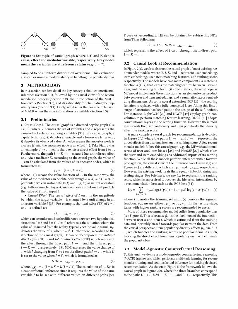
Figure 4: Example of causal graph where I, Y, and K denotecause, effect andmediator variable, respectively. Gray nodesmean the variables are at reference status (e.g., 𝐼 = 𝑖∗).

sampled to be a uniform distribution over items. This evaluationalso can examine a model’s ability in handling the popularity bias.

3 METHODOLOGYIn this section, we first detail the key concepts about counterfactualinference (Section 3.1), followed by the causal view of the recom-mendation process (Section 3.2), the introduction of the MACRframework (Section 3.3), and its rationality for eliminating the pop-ularity bias (Section 3.4). Lastly, we discuss the possible extensionof MACR when the side information is available (Section 3.5).

3.1 Preliminaries• Causal Graph. The causal graph is a directed acyclic graph 𝐺 =

{𝑉 , 𝐸}, where 𝑉 denotes the set of variables and 𝐸 represents thecause-effect relations among variables [35]. In a causal graph, acapital letter (e.g., 𝐼 ) denotes a variable and a lowercase letter (e.g.,𝑖) denotes its observed value. An edge means the ancestor node isa cause (𝐼 ) and the successor node is an effect (𝑌 ). Take Figure 4 asan example, 𝐼 → 𝑌 means there exists a direct effect from 𝐼 to 𝑌 .Furthermore, the path 𝐼 → 𝐾 → 𝑌 means 𝐼 has an indirect effecton 𝑌 via a mediator 𝐾 . According to the causal graph, the value of𝑌 can be calculated from the values of its ancestor nodes, which isformulated as:

𝑌𝑖,𝑘 = 𝑌 (𝐼 = 𝑖, 𝐾 = 𝑘), (2)where 𝑌 (.) means the value function of 𝑌 . In the same way, thevalue of the mediator can be obtained through 𝑘 = 𝐾𝑖 = 𝐾 (𝐼 = 𝑖). Inparticular, we can instantiate 𝐾 (𝐼 ) and 𝑌 (𝐼 , 𝐾) as neural operators(e.g., fully-connected layers), and compose a solution that predictsthe value of Y from input I.

• Causal Effect. The causal effect of 𝐼 on 𝑌 is the magnitudeby which the target variable 𝑌 is changed by a unit change in anancestor variable 𝐼 [35]. For example, the total effect (TE) of 𝐼 = 𝑖on 𝑌 is defined as:

𝑇𝐸 = 𝑌𝑖,𝐾𝑖− 𝑌𝑖∗,𝐾𝑖∗ , (3)

which can be understood as the difference between two hypotheticalsituations 𝐼 = 𝑖 and 𝐼 = 𝑖∗. 𝐼 = 𝑖∗ refers to a the situation where thevalue of 𝐼 is muted from the reality, typically set the value as null.𝐾𝑖∗denotes the value of 𝐾 when 𝐼 = 𝑖∗. Furthermore, according to thestructure of the causal graph, TE can be decomposed into naturaldirect effect (NDE) and total indirect effect (TIE) which representthe effect through the direct path 𝐼 → 𝑌 and the indirect path𝐼 → 𝐾 → 𝑌 , respectively [35]. NDE expresses the value change of𝑌 with 𝐼 changing from 𝑖∗ to 𝑖 on the direct path 𝐼 → 𝑌 , while 𝐾is set to the value when 𝐼 = 𝑖∗, which is formulated as:

𝑁𝐷𝐸 = 𝑌𝑖,𝐾𝑖∗ − 𝑌𝑖∗,𝐾𝑖∗ , (4)where 𝑌𝑖,𝐾𝑖∗ = 𝑌 (𝐼 = 𝑖, 𝐾 = 𝐾 (𝐼 = 𝑖∗)). The calculation of 𝑌𝑖 , 𝐾𝑖∗ isa counterfactual inference since it requires the value of the samevariable 𝐼 to be set with different values on different paths (see

Figure 4). Accordingly, TIE can be obtained by subtracting NDEfrom TE as following:

𝑇 𝐼𝐸 = 𝑇𝐸 − 𝑁𝐷𝐸 = 𝑌𝑖,𝐾𝑖− 𝑌𝑖,𝐾𝑖∗ , (5)

which represents the effect of 𝐼 on 𝑌 through the indirect path𝐼 → 𝐾 → 𝑌 .

3.2 Causal Look at RecommendationIn Figure 2(a), we first abstract the causal graph of most existing rec-ommender models, where𝑈 , 𝐼 , 𝐾 , and 𝑌 represent user embedding,item embedding, user-item matching features, and ranking score,respectively. The models have two main components: a matchingfunction𝐾 (𝑈 , 𝐼 ) that learns thematching features between user anditem; and the scoring function 𝑌 (𝐾). For instance, the most popularMF model implements these functions as an element-wise productbetween user and item embeddings, and a summation across embed-ding dimensions. As to its neural extension NCF [22], the scoringfunction is replaced with a fully-connected layer. Along this line, asurge of attention has been paid to the design of these functions.For instance, LightGCN [20] and NGCF [49] employ graph con-volution to perform matching feature learning, ONCF [21] adoptsconvolutional layers as the scoring function. However, these mod-els discards the user conformity and item popularity that directlyaffect the ranking score.

A more complete causal graph for recommendation is depictedin Figure 2(c) where the paths 𝑈 → 𝑌 and 𝐼 → 𝑌 represent thedirect effects from user and item on the ranking score. A few recom-mender models follow this causal graph, e.g., the MFwith additionalterms of user and item biases [28] and NeuMF [22] which takesthe user and item embeddings as additional inputs of its scoringfunction. While all these models perform inference with a forwardpropagation, the causal view of the inference over Figure 2(a) andFigure 2(c) are different, which are 𝑌𝐾𝑢,𝑖 and 𝑌𝑢,𝑖,𝐾𝑢,𝑖 , respectively.However, the existing work treats them equally in both training andtesting stages. For briefness, we use 𝑦𝑢𝑖 to represent the rankingscore, which is supervised to recover the historical interactions bya recommendation loss such as the BCE loss [54]:𝐿𝑂 =

∑(𝑢,𝑖) ∈𝐷

−𝑦𝑢𝑖 log(𝜎 (𝑦𝑢𝑖 )) − (1 − 𝑦𝑢𝑖 ) log(1 − 𝜎 (𝑦𝑢𝑖 )), (6)

where 𝐷 denotes the training set and 𝜎 (·) denotes the sigmoidfunction. 𝑦𝑢,𝑖 means either 𝑌𝐾𝑢,𝑖 or 𝑌𝑢,𝑖,𝐾𝑢,𝑖 . In the testing stage,items with higher ranking scores are recommended to users.

Most of these recommender model suffer from popularity bias(see Figure 1). This is because𝑦𝑢𝑖 is the likelihood of the interactionbetween user 𝑢 and item 𝑖 , which is estimated from the trainingdata and inevitably biased towards popular items in the data. Fromthe causal perspective, item popularity directly affects 𝑦𝑢𝑖 via 𝐼 →𝑌 , which bubbles the ranking scores of popular items. As such,blocking the direct effect from item popularity on 𝑌 will eliminatethe popularity bias.

3.3 Model-Agnostic Counterfactual ReasoningTo this end, we devise a model-agnostic counterfactual reasoning(MACR) framework, which performs multi-task learning for recom-mender training and counterfactual inference for making debiasedrecommendation. As shown in Figure 5, the framework follows thecausal graph in Figure 2(c), where the three branches correspondto the paths𝑈 → 𝑌 ,𝑈&𝐼 → 𝐾 → 𝑌 , and 𝐼 → 𝑌 , respectively. This

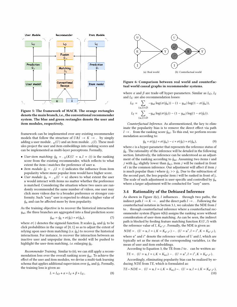
Figure 5: The framework of MACR. The orange rectanglesdenote themain branch, i.e., the conventional recommendersystem. The blue and green rectangles denote the user anditem modules, respectively.

framework can be implemented over any existing recommendermodels that follow the structure of 𝑈&𝐼 → 𝐾 → 𝑌 by simplyadding a user module 𝑌𝑢 (𝑈 ) and an item module 𝑌𝑖 (𝐼 ). These mod-ules project the user and item embeddings into ranking scores andcan be implemented as multi-layer perceptrons. Formally,

• User-item matching: 𝑦𝑘 = 𝑌𝑘 (𝐾 (𝑈 = 𝑢, 𝐼 = 𝑖)) is the rankingscore from the existing recommender, which reflects to whatextent the item 𝑖 matches the preference of user 𝑢.

• Item module: 𝑦𝑖 = 𝑌𝑖 (𝐼 = 𝑖) indicates the influence from itempopularity where more popular item would have higher score.

• User module: 𝑦𝑢 = 𝑌𝑢 (𝑈 = 𝑢) shows to what extent the user𝑢 would interact with items no matter whether the preferenceis matched. Considering the situation where two users are ran-domly recommended the same number of videos, one user mayclick more videos due to a broader preference or stronger con-formity. Such “easy” user is expected to obtain a higher value of𝑦𝑢 and can be affected more by item popularity.

As the training objective is to recover the historical interactions𝑦𝑢𝑖 , the three branches are aggregated into a final prediction score:

𝑦𝑢𝑖 = 𝑦𝑘 ∗ 𝜎 (𝑦𝑖 ) ∗ 𝜎 (𝑦𝑢 ), (7)where 𝜎 (·) denotes the sigmoid function. It scales 𝑦𝑢 and 𝑦𝑖 to beclick probabilities in the range of [0, 1] so as to adjust the extent ofrelying upon user-item matching (i.e. 𝑦𝑘 ) to recover the historicalinteractions. For instance, to recover the interaction between aninactive user and unpopular item, the model will be pushed tohighlight the user-item matching, i.e. enlarging 𝑦𝑘 .

Recommender Training. Similar to (6), we can still apply a recom-mendation loss over the overall ranking score 𝑦𝑢𝑖 . To achieve theeffect of the user and item modules, we devise a multi-task learningschema that applies additional supervision over𝑦𝑢 and𝑦𝑖 . Formally,the training loss is given as:

𝐿 = 𝐿𝑂 + 𝛼 ∗ 𝐿𝐼 + 𝛽 ∗ 𝐿𝑈 , (8)

(a) Real world (b) Conterfactual world

Figure 6: Comparison between real world and counterfac-tual world causal graphs in recommender systems.

where 𝛼 and 𝛽 are trade-off hyper-parameters. Similar as 𝐿𝑂 , 𝐿𝐼and 𝐿𝑈 are also recommendation losses:

𝐿𝑈 =∑

(𝑢,𝑖) ∈𝐷−𝑦𝑢𝑖 log(𝜎 (𝑦𝑢 )) − (1 − 𝑦𝑢𝑖 ) log(1 − 𝜎 (𝑦𝑢 )),

𝐿𝐼 =∑

(𝑢,𝑖) ∈𝐷−𝑦𝑢𝑖 log(𝜎 (𝑦𝑖 )) − (1 − 𝑦𝑢𝑖 ) log(1 − 𝜎 (𝑦𝑖 )).

Counterfactual Inference. As aforementioned, the key to elim-inate the popularity bias is to remove the direct effect via path𝐼 → 𝑌 from the ranking score 𝑦𝑢𝑖 . To this end, we perform recom-mendation according to:

𝑦𝑘 ∗ 𝜎 (𝑦𝑖 ) ∗ 𝜎 (𝑦𝑢 ) − 𝑐 ∗ 𝜎 (𝑦𝑖 ) ∗ 𝜎 (𝑦𝑢 ), (9)where 𝑐 is a hyper-parameter that represents the reference status of𝑦𝑘 . The rationality of the inference will be detailed in the followingsection. Intuitively, the inference can be understood as an adjust-ment of the ranking according to 𝑦𝑢𝑖 . Assuming two items 𝑖 and𝑗 with 𝑦𝑢𝑖 slightly lower than 𝑦𝑢 𝑗 , item 𝑗 will be ranked in frontof 𝑖 in the common inference. Our adjustment will affect if item 𝑗

is much popular than 𝑖 where 𝑦 𝑗 >> 𝑦𝑖 . Due to the subtraction ofthe second part, the less popular item 𝑖 will be ranked in front of j..The scale of such adjustment is user-specific and controlled by 𝑦𝑢where a larger adjustment will be conducted for “easy” users.

3.4 Rationality of the Debiased InferenceAs shown in Figure 2(c), 𝐼 influences 𝑌 through two paths, theindirect path 𝐼 → 𝐾 → 𝑌 and the direct path 𝐼 → 𝑌 . Following thecounterfactual notation in Section 3.1, we calculate the NDE from 𝐼

to 𝑌 through counterfactual inference where a counterfactual rec-ommender system (Figure 6(b)) assigns the ranking score withoutconsideration of user-item matching. As can be seen, the indirectpath is blocked by feeding feature matching function 𝐾 (𝑈 , 𝐼 ) withthe reference value of 𝐼 , 𝐾𝑢∗,𝑖∗ . Formally, the NDE is given as:𝑁𝐷𝐸 = 𝑌 (𝑈 = 𝑢, 𝐼 = 𝑖, 𝐾 = 𝐾𝑢∗,𝑖∗ ) − 𝑌 (𝑈 = 𝑢∗, 𝐼 = 𝑖∗, 𝐾 = 𝐾𝑢∗,𝑖∗ ),where 𝑢∗ and 𝑖∗ denote the reference values of𝑈 and 𝐼 , which aretypically set as the mean of the corresponding variables, i.e. themean of user and item embeddings.

According to Equation 3, the TE from 𝐼 to 𝑌 can be written as:𝑇𝐸 = 𝑌 (𝑈 = 𝑢, 𝐼 = 𝑖, 𝐾 = 𝐾𝑢,𝑖 ) − 𝑌 (𝑈 = 𝑢∗, 𝐼 = 𝑖∗, 𝐾 = 𝐾𝑢∗,𝑖∗ ) .Accordingly, eliminating popularity bias can be realized by re-

ducing 𝑁𝐷𝐸 from 𝑇𝐸, which is formulated as:𝑇𝐸−𝑁𝐷𝐸 = 𝑌 (𝑈 = 𝑢, 𝐼 = 𝑖, 𝐾 = 𝐾𝑢,𝑖 ) −𝑌 (𝑈 = 𝑢, 𝐼 = 𝑖, 𝐾 = 𝐾𝑢∗,𝑖∗ ),

(10)

Table 1: Statistics of five different datasets.

Users Items Interactions SparsityAdressa 13,485 744 116,321 0.011594Globo 158,323 12,005 2,520,171 0.001326ML10M 69,166 8,790 5,000,415 0.008225Yelp 31,668 38,048 1,561,406 0.001300Gowalla 29,858 40,981 1,027,370 0.000840

Recall that the ranking score is calculated according to Equation 7.As such, we have 𝑌 (𝑈 = 𝑢, 𝐼 = 𝑖, 𝐾 = 𝐾𝑢,𝑖 ) = 𝑦𝑘 ∗𝜎 (𝑦𝑖 ) ∗𝜎 (𝑦𝑢 ) and𝑌 (𝑈 = 𝑢, 𝐼 = 𝑖, 𝐾 = 𝐾𝑢∗,𝑖∗ ) = 𝑐 ∗ 𝜎 (𝑦𝑖 ) ∗ 𝜎 (𝑦𝑢 ) where 𝑐 denotes thevalue𝑦𝑘 with𝐾 = 𝐾𝑢∗,𝑖∗ . In this way, we obtain the ranking schemafor the testing stage as Equation 9. Recall that𝑇 𝐼𝐸 = 𝑇𝐸−𝑁𝐷𝐸, thekey difference of the proposed counterfactual inference and normalinference is using TIE to rank items rather than TE. Algorithm inAppendix A describes the procedure of our method.

3.5 DiscussionThere are usually multiple causes for one item click, such as items’popularity, category, and quality. In this work, we focus on the biasrevealed by the interaction frequency. As an initial attempt to solvethe problem from the perspective of cause-effect, we ignoring theeffect of other factors. Due to the unavailability of side informa-tion [39] on such factors or the exposure mechanism to uncoverdifferent causes for the recommendation, it is also non-trivial toaccount for such factors.

As we can access such side information, we can simply extendthe proposed MACR framework by incorporating such informationinto the causal graph as additional nodes. Then we can reveal thereasons that cause specific recommendations and try to furthereliminate the bias, which is left for future exploration.

4 EXPERIMENTSIn this section, we conduct experiments to evaluate the performanceof our proposed MACR. Our experiments are intended to answerthe following research questions:• RQ1: Does MACR outperform existing debiasing methods?• RQ2: How do different hyper-parameter settings (e.g. 𝛼, 𝛽, 𝑐)affect the recommendation performance?

• RQ3:How do different components in our framework contributeto the performance?

• RQ4: How does MACR eliminate the popularity bias?

4.1 Experiment SettingsDatasets. Five real-world benchmark datasets are used in our

experiments: ML10M is the widely-used [6, 40, 59] dataset fromMovieLens with 10M movie ratings. While it is an explicit feed-back dataset, we have intentionally chosen it to investigate theperformance of learning from the implicit signal. To this end, wetransformed it into implicit data, where each entry is marked as 0or 1 indicating whether the user has rated the item; Adressa [18]and Globo [14] are two popular datasets for news recommendation;Also, the datasets Gowalla and Yelp from LightGCN [20] are usedfor a fair comparison. All the datasets above are publicly availableand vary in terms of domain, size, and sparsity. The statistics ofthese datasets are summarized in Table 1.

Evaluation. Note that the conventional evaluation strategy ona set of holdout interactions does not reflect the ability to pre-dict user’s preference, as it still follows the long tail distribution[58]. Consequently, the test model can still perform well even if itonly considers popularity and ignores users’ preference [58]. Thus,the conventional evaluation strategy is not appropriate for test-ing whether the model suffers from popularity bias, and we needto evaluate on the debiased data. To this end, we follow previousworks [7, 30, 58] to simulate debiased recommendation where thetesting interactions are sampled to be a uniform distribution overitems. In particular, we randomly sample 10% interactions withequal probability in terms of items as the test set, another 10% asthe validation set, and leave the others as the biased training data1.We report the all-ranking performance w.r.t. three widely used met-rics: Hit Ratio (HR), Recall, and Normalized Discounted CumulativeGain (NDCG) cut at 𝐾 .

4.1.1 Baselines. We implement our MACR with the classic MF(MACR_MF) and the state-of-the-art LightGCN (MACR_LightGCN)to explore how MACR boosts recommendation performance. Wecompare our methods with the following baselines:• MF [28]: This is a representative collaborative filtering modelas formulated in Section 3.2.

• LightGCN [20]: This is the state-of-the-art collaborative filter-ing recommendation model based on light graph convolution asillustrated in Section 3.2.

• ExpoMF [31]: A probabilistic model that separately estimatesthe user preferences and the exposure.

• CausE_MF, CausE_LightGCN [7]: CausE is a domain adapta-tion algorithm that learns from debiased datasets to benefit thebiased training. In our experiments, we separate the training setinto debiased and biased ones to implement this method. Further,we apply CausE into two recommendation models (i.e. MF andLightGCN) for fair comparisons. Similar treatments are used forthe following debias strategy.

• BS_MF, BS_LightGCN [28]: BS learns a biased score from thetraining stage and then remove the bias in the prediction in thetesting stage. The prediction function is defined as:𝑦𝑢𝑖 = 𝑦𝑘 + 𝑏𝑖 ,where 𝑏𝑖 is the bias term of the item 𝑖 .

• Reg_MF, Reg_LightGCN [2]: Reg is a regularization-basedapproach that intentionally downweights the short tail items,covers more items, and thus improves long tail recommendation.

• IPW_MF, IPW_LightGCN: [30, 42] IPW Adds the standardInverse Propensity Weight to reweight samples to alleviate itempopularity bias.

• DICE_MF, DICE_LightGCN: [58] This is a state-of-the-artmethod for learning causal embedding to cope with popular-ity bias problem. It designs a framework with causal-specific datato disentangle interest and popularity into two sets of embedding.We used the code provided by its authors.

As we aim to model the interactions between users and items, wedo not compare with models that use side information. We leaveout the comparison with other collaborative filtering models, suchas NeuMF [22] and NGCF [49], because LightGCN [20] is the state-of-the-art collaborative filtering method at present. Implementationdetails and detailed parameter settings of the models can be foundin Appendix B.

1We refer to [7, 30, 58] for details on extracting an debiased test set from biased data.

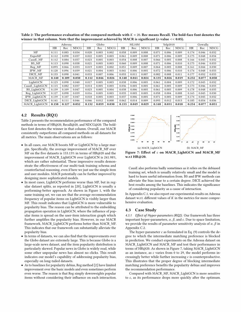
Table 2: The performance evaluation of the compared methods with 𝐾 = 20. Rec means Recall. The bold-face font denotes thewinner in that column. Note that the improvement achieved by MACR is significant (𝑝-value << 0.05).

Adressa Globo ML10M Yelp2018 GowallaHR Rec NDCG HR Rec NDCG HR Rec NDCG HR Rec NDCG HR Rec NDCG

MF 0.111 0.085 0.034 0.020 0.003 0.002 0.058 0.009 0.008 0.071 0.006 0.009 0.174 0.046 0.032ExpoMF 0.112 0.090 0.037 0.022 0.005 0.003 0.061 0.009 0.008 0.071 0.006 0.009 0.175 0.048 0.034CausE_MF 0.112 0.084 0.037 0.023 0.005 0.003 0.054 0.008 0.007 0.066 0.005 0.008 0.166 0.045 0.032BS_MF 0.113 0.090 0.038 0.021 0.005 0.003 0.060 0.009 0.008 0.071 0.006 0.010 0.175 0.046 0.033Reg_MF 0.093 0.066 0.033 0.019 0.003 0.002 0.051 0.009 0.007 0.064 0.005 0.008 0.161 0.044 0.030IPW_MF 0.128 0.096 0.039 0.021 0.004 0.003 0.041 0.006 0.005 0.072 0.006 0.010 0.174 0.048 0.033DICE_MF 0.133 0.098 0.041 0.033 0.007 0.006 0.055 0.011 0.007 0.082 0.008 0.011 0.177 0.052 0.033MACR_MF 0.140 0.109 0.050 0.112 0.046 0.026 0.140 0.041 0.024 0.135 0.026 0.019 0.252 0.077 0.050LightGCN 0.123 0.098 0.040 0.017 0.005 0.003 0.038 0.006 0.005 0.061 0.004 0.009 0.172 0.045 0.032

CausE_LightGCN 0.115 0.082 0.037 0.014 0.005 0.003 0.036 0.005 0.005 0.061 0.005 0.009 0.173 0.046 0.033BS_LightGCN 0.139 0.109 0.047 0.023 0.005 0.004 0.038 0.006 0.005 0.061 0.005 0.009 0.178 0.048 0.035Reg_LightGCN 0.127 0.098 0.039 0.016 0.005 0.003 0.035 0.005 0.005 0.058 0.004 0.008 0.165 0.045 0.030IPW_LightGCN 0.139 0.107 0.047 0.018 0.005 0.003 0.037 0.006 0.005 0.071 0.005 0.009 0.174 0.045 0.032DICE_LightGCN 0.141 0.111 0.046 0.046 0.012 0.008 0.062 0.014 0.009 0.093 0.012 0.013 0.185 0.054 0.036MACR_LightGCN 0.158 0.127 0.052 0.132 0.059 0.030 0.155 0.049 0.029 0.148 0.031 0.018 0.254 0.077 0.051

4.2 Results (RQ1)Table 2 presents the recommendation performance of the comparedmethods in terms of HR@20, Recall@20, and NDCG@20. The bold-face font denotes the winner in that column. Overall, our MACRconsistently outperforms all compared methods on all datasets forall metrics. The main observations are as follows:

• In all cases, our MACR boosts MF or LightGCN by a large mar-gin. Specifically, the average improvement of MACR_MF overMF on the five datasets is 153.13% in terms of HR@20 and theimprovement of MACR_LightGCN over LightGCN is 241.98%,which are rather substantial. These impressive results demon-strate the effectiveness of our multi-task training schema andcounterfactual reasoning, even if here we just use the simple itemand user modules. MACR potentially can be further improved bydesigning more sophisticated models.

• In most cases, LightGCN performs worse than MF, but in reg-ular dataset splits, as reported in [20], LightGCN is usually aperforming-better approach. As shown in Figure 1, with thesame training set, we can see that the average recommendationfrequency of popular items on LightGCN is visibly larger thanMF. This result indicates that LightGCN is more vulnerable topopularity bias. The reason can be attributed to the embeddingpropagation operation in LightGCN, where the influence of pop-ular items is spread on the user-item interaction graph whichfurther amplifies the popularity bias. However, in our MACRframework, MACR_LightGCN performs better than MACR_MF.This indicates that our framework can substantially alleviate thepopularity bias.

• In terms of datasets, we can also find that the improvements overthe Globo dataset are extremely large. This is because Globo is alarge-scale news dataset, and the item popularity distribution isparticularly skewed. Popular news in Globo is widely read, whilesome other unpopular news has almost no clicks. This resultindicates our model’s capability of addressing popularity bias,especially on long-tailed datasets.

• As to baselines for popularity debias, Reg method [2] have limitedimprovement over the basic models and even sometimes performeven worse. The reason is that Reg simply downweights popularitems without considering their influence on each interaction.

(a) MACR_LightGCN (b) MACR_MF

Figure 7: Effect of 𝑐 on MACR_LightGCN and MACR_MFw.r.t HR@20.

CausE also performs badly sometimes as it relies on the debiasedtraining set, which is usually relatively small and the model ishard to learn useful information from. BS and IPW methods canalleviate the bias issue to a certain degree. DICE achieved thebest results among the baselines. This indicates the significanceof considering popularity as a cause of interaction.

In Appendix C.1, we also report our experimental results on Adressadataset w.r.t. different values of 𝐾 in the metrics for more compre-hensive evaluation.

4.3 Case Study4.3.1 Effect of Hyper-parameters (RQ2). Our framework has threeimportant hyper-parameters, 𝛼 , 𝛽 , and 𝑐 . Due to space limitation,we provide the results of parameter sensitivity analysis of 𝛼 , 𝛽 inAppendix C.2.

The hyper-parameter 𝑐 as formulated in Eq. (9) controls the de-gree to which the intermediate matching preference is blockedin prediction. We conduct experiments on the Adressa dataset onMACR_LightGCN and MACR_MF and test their performance interms of HR@20. As shown in Figure 7, taking MACR_LightGCNas an instance, as 𝑐 varies from 0 to 29, the model performs in-creasingly better while further increasing 𝑐 is counterproductive.This illustrates that the proper degree of blocking intermediatematching preference benefits the popularity debias and improvesthe recommendation performance.

Compared with MACR_MF, MACR_LightGCN is more sensitiveto 𝑐 , as its performance drops more quickly after the optimum.

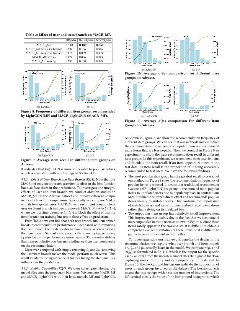
Table 3: Effect of user and item branch on MACR_MF.HR@20 Recall@20 NDCG@20

MACR_MF 0.140 0.109 0.050MACR_MF w/o user branch 0.137 0.106 0.046MACR_MF w/o item branch 0.116 0.089 0.038

MACR_MF w/o 𝐿𝐼 0.124 0.096 0.043MACR_MF w/o 𝐿𝑈 0.138 0.108 0.048

(a) LightGCN (b) MF

Figure 8: Frequency of different item groups recommendedby LightGCN (MF) and MACR_LightGCN (MACR_MF).

(a) LightGCN (b) MF

Figure 9: Average item recall in different item groups onAdressa.It indicates that LightGCN is more vulnerable to popularity bias,which is consistent with our findings in Section 4.2.

4.3.2 Effect of User Branch and Item Branch (RQ3). Note that ourMACR not only incorporates user/item’s effect in the loss functionbut also fuse them in the predictions. To investigate the integraleffects of user and item branch, we conduct ablation studies onMACR_MF on the Adressa dataset and remove different compo-nents at a time for comparisons. Specifically, we compare MACRwith its four special cases: MACR_MFw/o user (item) branch, whereuser (or item) branch has been removed; MACR_MF w/o 𝐿𝐼 (𝐿𝑈 ),where we just simply remove 𝐿𝐼 (𝐿𝑈 ) to block the effect of user (oritem) branch on training but retain their effect on prediction.

From Table 3 we can find that both user branch and item branchboosts recommendation performance. Compared with removingthe user branch, the model performs much worse when removingthe item branch. Similarly, compared with removing 𝐿𝑈 , removing𝐿𝐼 also harms the performance more heavily. This result validatesthat item popularity bias has more influence than user conformityon the recommendation.

Moreover, compared with simply removing 𝐿𝐼 and 𝐿𝑈 , removingthe user/item branch makes the model perform much worse. Thisresult validates the significance of further fusing the item and userinfluence in the prediction.

4.3.3 Debias Capability (RQ4). We then investigate whether ourmodel alleviates the popularity bias issue. We compare MACR_MFand MACR_LightGCN with their basic models, MF and LightGCN.

(a) LightGCN (b) MFFigure 10: Average 𝜎 (𝑦𝑢 ) comparison for different usergroups on Adressa.

(a) LightGCN (b) MF

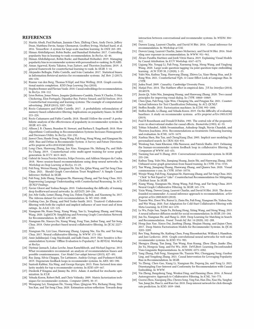
Figure 11: Average 𝜎 (𝑦𝑖 ) comparison for different itemgroups on Adressa.

As shown in Figure 8, we show the recommendation frequency ofdifferent item groups. We can see that our methods indeed reducethe recommendations frequency of popular items and recommendmore items that are less popular. Then we conduct in Figure 9 anexperiment to show the item recommendation recall in differentitem groups. In this experiment, we recommend each user 20 itemsand calculate the item recall. If an item appears 𝑁 times in thetest data, its item recall is the proportion of it being accuratelyrecommended to test users. We have the following findings.• The most popular item group has the greatest recall increase, butour methods in Figure 8 show the recommendations frequency ofpopular items is reduced. It means that traditional recommendersystems (MF, LightGCN) are prone to recommend more popularitems to unrelated users due to popularity bias. In contrast, ourMACR reduces the item’s direct effect and recommends popularitems mainly to suitable users. This confirms the importanceof matching users and items for personalized recommendationsrather than relying on item related bias.

• The unpopular item group has relatively small improvement.This improvement is mainly due to the fact that we recommendmore unpopular items to users as shown in Figure 8. Since theseitems rarely appear in the training set, it is difficult to obtain acomprehensive representation of these items, so it is difficult togain a large improvement in our method.To investigate why our framework benefits the debias in the

recommendation, we explore what user branch and item branch,i.e., 𝑦𝑢 and 𝑦𝑖 , actually learn in the model. We compare 𝜎 (𝑦𝑢 ) and𝜎 (𝑦𝑖 ) as formulated in Eq. (7) , which is the output for the specificuser𝑢 or item 𝑖 from the user/itemmodel after the sigmoid function,capturing user conformity and item popularity in the dataset. InFigure 10, the background histograms indicate the proportion ofusers in each group involved in the dataset. The horizontal axismeans the user groups with a certain number of interactions. Theleft vertical axis is the value of the background histograms, which

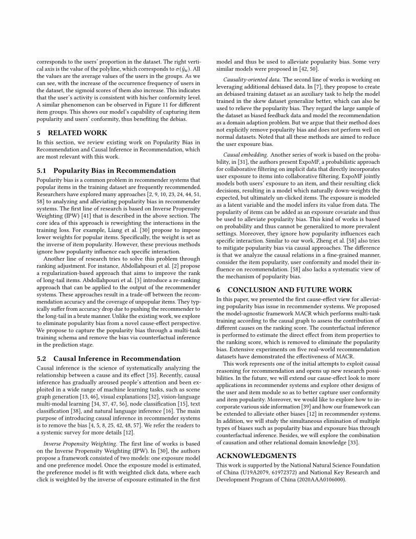
corresponds to the users’ proportion in the dataset. The right verti-cal axis is the value of the polyline, which corresponds to 𝜎 (𝑦𝑢 ). Allthe values are the average values of the users in the groups. As wecan see, with the increase of the occurrence frequency of users inthe dataset, the sigmoid scores of them also increase. This indicatesthat the user’s activity is consistent with his/her conformity level.A similar phenomenon can be observed in Figure 11 for differentitem groups. This shows our model’s capability of capturing itempopularity and users’ conformity, thus benefiting the debias.

5 RELATEDWORKIn this section, we review existing work on Popularity Bias inRecommendation and Causal Inference in Recommendation, whichare most relevant with this work.

5.1 Popularity Bias in RecommendationPopularity bias is a common problem in recommender systems thatpopular items in the training dataset are frequently recommended.Researchers have explored many approaches [2, 9, 10, 23, 24, 44, 51,58] to analyzing and alleviating popularity bias in recommendersystems. The first line of research is based on Inverse PropensityWeighting (IPW) [41] that is described in the above section. Thecore idea of this approach is reweighting the interactions in thetraining loss. For example, Liang et al. [30] propose to imposelower weights for popular items. Specifically, the weight is set asthe inverse of item popularity. However, these previous methodsignore how popularity influence each specific interaction.

Another line of research tries to solve this problem throughranking adjustment. For instance, Abdollahpouri et al. [2] proposea regularization-based approach that aims to improve the rankof long-tail items. Abdollahpouri et al. [3] introduce a re-rankingapproach that can be applied to the output of the recommendersystems. These approaches result in a trade-off between the recom-mendation accuracy and the coverage of unpopular items. They typ-ically suffer from accuracy drop due to pushing the recommender tothe long-tail in a brute manner. Unlike the existing work, we exploreto eliminate popularity bias from a novel cause-effect perspective.We propose to capture the popularity bias through a multi-tasktraining schema and remove the bias via counterfactual inferencein the prediction stage.

5.2 Causal Inference in RecommendationCausal inference is the science of systematically analyzing therelationship between a cause and its effect [35]. Recently, causalinference has gradually aroused people’s attention and been ex-ploited in a wide range of machine learning tasks, such as scenegraph generation [13, 46], visual explanations [32], vision-languagemulti-modal learning [34, 37, 47, 56], node classification [15], textclassification [38], and natural language inference [16]. The mainpurpose of introducing causal inference in recommender systemsis to remove the bias [4, 5, 8, 25, 42, 48, 57]. We refer the readers toa systemic survey for more details [12].

Inverse Propensity Weighting. The first line of works is basedon the Inverse Propensity Weighting (IPW). In [30], the authorspropose a framework consisted of two models: one exposure modeland one preference model. Once the exposure model is estimated,the preference model is fit with weighted click data, where eachclick is weighted by the inverse of exposure estimated in the first

model and thus be used to alleviate popularity bias. Some verysimilar models were proposed in [42, 50].

Causality-oriented data. The second line of works is working onleveraging additional debiased data. In [7], they propose to createan debiased training dataset as an auxiliary task to help the modeltrained in the skew dataset generalize better, which can also beused to relieve the popularity bias. They regard the large sample ofthe dataset as biased feedback data and model the recommendationas a domain adaption problem. But we argue that their method doesnot explicitly remove popularity bias and does not perform well onnormal datasets. Noted that all these methods are aimed to reducethe user exposure bias.

Causal embedding. Another series of work is based on the proba-bility, in [31], the authors present ExpoMF, a probabilistic approachfor collaborative filtering on implicit data that directly incorporatesuser exposure to items into collaborative filtering. ExpoMF jointlymodels both users’ exposure to an item, and their resulting clickdecisions, resulting in a model which naturally down-weights theexpected, but ultimately un-clicked items. The exposure is modeledas a latent variable and the model infers its value from data. Thepopularity of items can be added as an exposure covariate and thusbe used to alleviate popularity bias. This kind of works is basedon probability and thus cannot be generalized to more prevalentsettings. Moreover, they ignore how popularity influences eachspecific interaction. Similar to our work, Zheng et al. [58] also triesto mitigate popularity bias via causal approaches. The differenceis that we analyze the causal relations in a fine-grained manner,consider the item popularity, user conformity and model their in-fluence on recommendation. [58] also lacks a systematic view ofthe mechanism of popularity bias.

6 CONCLUSION AND FUTUREWORKIn this paper, we presented the first cause-effect view for alleviat-ing popularity bias issue in recommender systems. We proposedthe model-agnostic framework MACR which performs multi-tasktraining according to the causal graph to assess the contribution ofdifferent causes on the ranking score. The counterfactual inferenceis performed to estimate the direct effect from item properties tothe ranking score, which is removed to eliminate the popularitybias. Extensive experiments on five real-world recommendationdatasets have demonstrated the effectiveness of MACR.

This work represents one of the initial attempts to exploit causalreasoning for recommendation and opens up new research possi-bilities. In the future, we will extend our cause-effect look to moreapplications in recommender systems and explore other designs ofthe user and item module so as to better capture user conformityand item popularity. Moreover, we would like to explore how to in-corporate various side information [39] and how our framework canbe extended to alleviate other biases [12] in recommender systems.In addition, we will study the simultaneous elimination of multipletypes of biases such as popularity bias and exposure bias throughcounterfactual inference. Besides, we will explore the combinationof causation and other relational domain knowledge [33].

ACKNOWLEDGMENTSThis work is supported by the National Natural Science Foundationof China (U19A2079, 61972372) and National Key Research andDevelopment Program of China (2020AAA0106000).

REFERENCES[1] Martín Abadi, Paul Barham, Jianmin Chen, Zhifeng Chen, Andy Davis, Jeffrey

Dean, Matthieu Devin, Sanjay Ghemawat, Geoffrey Irving, Michael Isard, et al.2016. Tensorflow: A system for large-scale machine learning. In OSDI. 265–283.

[2] Himan Abdollahpouri, Robin Burke, and Bamshad Mobasher. 2017. Controllingpopularity bias in learning-to-rank recommendation. In RecSys. 42–46.

[3] Himan Abdollahpouri, Robin Burke, and Bamshad Mobasher. 2019. Managingpopularity bias in recommender systemswith personalized re-ranking. In FLAIRS.

[4] Aman Agarwal, Kenta Takatsu, Ivan Zaitsev, and Thorsten Joachims. 2019. Ageneral framework for counterfactual learning-to-rank. In SIGIR. 5–14.

[5] Alejandro Bellogín, Pablo Castells, and Iván Cantador. 2017. Statistical biasesin Information Retrieval metrics for recommender systems. Inf. Retr. J. (2017),606–634.

[6] Rianne van den Berg, Thomas N Kipf, and Max Welling. 2018. Graph convolu-tional matrix completion. KDD Deep Learning Day (2018).

[7] Stephen Bonner and Flavian Vasile. 2018. Causal embeddings for recommendation.In RecSys. 104–112.

[8] Léon Bottou, Jonas Peters, Joaquin Quiñonero-Candela, Denis X Charles, D MaxChickering, Elon Portugaly, Dipankar Ray, Patrice Simard, and Ed Snelson. 2013.Counterfactual reasoning and learning systems: The example of computationaladvertising. JMLR (2013), 3207–3260.

[9] Rocío Cañamares and Pablo Castells. 2017. A probabilistic reformulation ofmemory-based collaborative filtering: Implications on popularity biases. In SIGIR.215–224.

[10] Rocío Cañamares and Pablo Castells. 2018. Should I follow the crowd? A proba-bilistic analysis of the effectiveness of popularity in recommender systems. InSIGIR. 415–424.

[11] Allison J. B. Chaney, Brandon M. Stewart, and Barbara E. Engelhardt. 2018. HowAlgorithmic Confounding in Recommendation Systems Increases Homogeneityand Decreases Utility. In RecSys. 224–232.

[12] Jiawei Chen, Hande Dong, XiangWang, Fuli Feng, MengWang, and Xiangnan He.2020. Bias and Debias in Recommender System: A Survey and Future Directions.arXiv preprint arXiv:2010.03240 (2020).

[13] Long Chen, Hanwang Zhang, Jun Xiao, Xiangnan He, Shiliang Pu, and Shih-Fu Chang. 2019. Counterfactual critic multi-agent training for scene graphgeneration. In ICCV. 4613–4623.

[14] Gabriel de Souza Pereira Moreira, Felipe Ferreira, and Adilson Marques da Cunha.2018. News session-based recommendations using deep neural networks. InWorkshop on Deep Learning at RecSys. 15–23.

[15] Fuli Feng, Weiran Huang, Xiangnan He, Xin Xin, QifanWang, and Tat-Seng ChuaChua. 2021. Should Graph Convolution Trust Neighbors? A Simple CausalInference Method. In SIGIR.

[16] Fuli Feng, Jizhi Zhang, Xiangnan He, Hanwang Zhang, and Tat-Seng Chua. 2021.Empowering Language Understanding with Counterfactual Reasoning. In ACL-IJCNLP Findings.

[17] Xavier Glorot and Yoshua Bengio. 2010. Understanding the difficulty of trainingdeep feedforward neural networks. In AISTATS. 249–256.

[18] Jon Atle Gulla, Lemei Zhang, Peng Liu, Özlem Özgöbek, and Xiaomeng Su. 2017.The Adressa dataset for news recommendation. In WI. 1042–1048.

[19] Guibing Guo, Jie Zhang, and Neil Yorke-Smith. 2015. Trustsvd: Collaborativefiltering with both the explicit and implicit influence of user trust and of itemratings.. In AAAI. 123–125.

[20] Xiangnan He, Kuan Deng, Xiang Wang, Yan Li, Yongdong Zhang, and MengWang. 2020. LightGCN: Simplifying and Powering Graph Convolution Networkfor Recommendation. In SIGIR. 639–648.

[21] Xiangnan He, Xiaoyu Du, Xiang Wang, Feng Tian, Jinhui Tang, and Tat-SengChua. 2018. Outer product-based neural collaborative filtering. In IJCAI. 2227–2233.

[22] Xiangnan He, Lizi Liao, Hanwang Zhang, Liqiang Nie, Xia Hu, and Tat-SengChua. 2017. Neural collaborative filtering. In WWW. 173–182.

[23] Amir Jadidinejad, Craig Macdonald, and Iadh Ounis. 2019. How Sensitive is Rec-ommendation Systems’ Offline Evaluation to Popularity?. In REVEAL Workshopat RecSys.

[24] Dietmar Jannach, Lukas Lerche, Iman Kamehkhosh, and Michael Jugovac. 2015.What recommenders recommend: an analysis of recommendation biases andpossible countermeasures. User Model User-adapt Interact (2015), 427–491.

[25] Ray Jiang, Silvia Chiappa, Tor Lattimore, András György, and Pushmeet Kohli.2019. Degenerate feedback loops in recommender systems. In AIES. 383–390.

[26] Santosh Kabbur, Xia Ning, and George Karypis. 2013. Fism: factored item simi-larity models for top-n recommender systems. In KDD. 659–667.

[27] Diederik P Kingma and Jimmy Ba. 2014. Adam: A method for stochastic opti-mization. In ICLR.

[28] Yehuda Koren, Robert Bell, and Chris Volinsky. 2009. Matrix factorization tech-niques for recommender systems. Computer (2009), 30–37.

[29] Wenqiang Lei, Xiangnan He, Yisong Miao, Qingyun Wu, Richang Hong, Min-Yen Kan, and Tat-Seng Chua. 2020. Estimation-action-reflection: Towards deep

interaction between conversational and recommender systems. In WSDM. 304–312.

[30] Dawen Liang, Laurent Charlin, and David M Blei. 2016. Causal inference forrecommendation. In Workshop at UAI.

[31] Dawen Liang, Laurent Charlin, James McInerney, and David M Blei. 2016. Mod-eling user exposure in recommendation. In WWW. 951–961.

[32] Álvaro Parafita Martínez and Jordi Vitrià Marca. 2019. Explaining Visual Modelsby Causal Attribution. In ICCV Workshop. 4167–4175.

[33] Liqiang Nie, Yongqi Li, Fuli Feng, Xuemeng Song, Meng Wang, and YinglongWang. 2020. Large-scale question tagging via joint question-topic embeddinglearning. ACM TOIS 38, 2 (2020), 1–23.

[34] Yulei Niu, Kaihua Tang, Hanwang Zhang, Zhiwu Lu, Xian-Sheng Hua, and Ji-Rong Wen. 2021. Counterfactual VQA: A Cause-Effect Look at Language Bias. InCVPR.

[35] Judea Pearl. 2009. Causality. Cambridge Uiversity Press.[36] Matjaž Perc. 2014. The Matthew effect in empirical data. J R Soc Interface (2014),

20140378.[37] Jiaxin Qi, Yulei Niu, Jianqiang Huang, and Hanwang Zhang. 2020. Two causal

principles for improving visual dialog. In CVPR. 10860–10869.[38] Chen Qian, Fuli Feng, Lijie Wen, Chunping Ma, and Pengjun Xie. 2021. Counter-

factual Inference for Text Classification Debiasing. In ACL-IJCNLP.[39] Steffen Rendle. 2010. Factorization machines. In ICDM. 995–1000.[40] Steffen Rendle, Li Zhang, and Yehuda Koren. 2019. On the difficulty of evaluating

baselines: A study on recommender systems. arXiv preprint arXiv:1905.01395(2019).

[41] Paul R Rosenbaum and Donald B Rubin. 1983. The central role of the propensityscore in observational studies for causal effects. Biometrika (1983), 41–55.

[42] Tobias Schnabel, Adith Swaminathan, Ashudeep Singh, Navin Chandak, andThorsten Joachims. 2016. Recommendations as treatments: Debiasing learningand evaluation. In ICML. 1670–1679.

[43] Xuehua Shen, Bin Tan, and ChengXiang Zhai. 2005. Implicit user modeling forpersonalized search. In CIKM. 824–831.

[44] Wenlong Sun, Sami Khenissi, Olfa Nasraoui, and Patrick Shafto. 2019. Debiasingthe human-recommender system feedback loop in collaborative filtering. InCompanion of WWW. 645–651.

[45] Yueming Sun and Yi Zhang. 2018. Conversational recommender system. In SIGIR.235–244.

[46] Kaihua Tang, Yulei Niu, Jianqiang Huang, Jiaxin Shi, and Hanwang Zhang. 2020.Unbiased scene graph generation from biased training. In CVPR. 3716–3725.

[47] Tan Wang, Jianqiang Huang, Hanwang Zhang, and Qianru Sun. 2020. Visualcommonsense r-cnn. In CVPR. 10760–10770.

[48] WenjieWang, Fuli Feng, XiangnanHe, Hanwang Zhang, and Tat-Seng Chua. 2021." Click" Is Not Equal to" Like": Counterfactual Recommendation for MitigatingClickbait Issue. In SIGIR.

[49] Xiang Wang, Xiangnan He, Meng Wang, Fuli Feng, and Tat-Seng Chua. 2019.Neural Graph Collaborative Filtering. In SIGIR. 165–174.

[50] Yixin Wang, Dawen Liang, Laurent Charlin, and David M Blei. 2018. The decon-founded recommender: A causal inference approach to recommendation. arXivpreprint arXiv:1808.06581 (2018).

[51] Tianxin Wei, Ziwei Wu, Ruirui Li, Ziniu Hu, Fuli Feng, Xiangnan He, Yizhou Sun,and Wei Wang. 2020. Fast Adaptation for Cold-Start Collaborative Filtering withMeta-Learning. In ICDM. 661–670.

[52] Le Wu, Peijie Sun, Yanjie Fu, Richang Hong, Xiting Wang, and Meng Wang. 2019.A neural influence diffusion model for social recommendation. In SIGIR. 235–244.

[53] Jun Xu, Xiangnan He, and Hang Li. 2020. Deep Learning for Matching in Searchand Recommendation. Found. Trends Inf. Ret. 14 (2020), 102–288.

[54] Hong-Jian Xue, Xinyu Dai, Jianbing Zhang, Shujian Huang, and Jiajun Chen.2017. Deep Matrix Factorization Models for Recommender Systems. In IJCAI.3203–3209.

[55] Rex Ying, Ruining He, Kaifeng Chen, Pong Eksombatchai, William L Hamilton,and Jure Leskovec. 2018. Graph convolutional neural networks for web-scalerecommender systems. In KDD. 974–983.

[56] Shengyu Zhang, Tan Jiang, Tan Wang, Kun Kuang, Zhou Zhao, Jianke Zhu,Jin Yu, Hongxia Yang, and Fei Wu. 2020. DeVLBert: Learning DeconfoundedVisio-Linguistic Representations. In ACMMM. 4373–4382.

[57] Yang Zhang, Fuli Feng, Xiangnan He, Tianxin Wei, Chonggang Song, GuohuiLing, and Yongdong Zhang. 2021. Causal Intervention for Leveraging PopularityBias in Recommendation. In SIGIR.

[58] Yu Zheng, Chen Gao, Xiang Li, Xiangnan He, Depeng Jin, and Yong Li. 2021.Disentangling User Interest and Conformity for Recommendation with CausalEmbedding. In WWW.

[59] Yin Zheng, Bangsheng Tang, Wenkui Ding, and Hanning Zhou. 2016. A NeuralAutoregressive Approach to Collaborative Filtering. In ICML. 764–773.

[60] Guorui Zhou, Xiaoqiang Zhu, Chenru Song, Ying Fan, Han Zhu, XiaoMa, YanghuiYan, Junqi Jin, Han Li, and Kun Gai. 2018. Deep interest network for click-throughrate prediction. In KDD. 1059–1068.

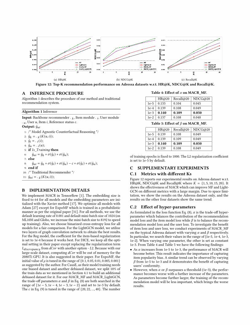
(a) HR@K (b) NDCG@K (c) Recall@K

Figure 12: Top-K recommendation performance on Adressa datasets w.r.t. HR@K, NDCG@K and Recall@K.

A INFERENCE PROCEDUREAlgorithm 1 describes the procedure of our method and traditionalrecommendation system.

Algorithm 1 InferenceInput: Backbone recommender 𝑌𝑘 , Item module 𝑌𝑖 , User module𝑌𝑢 , User 𝑢, Item 𝑖 , Reference status 𝑐 .Output: 𝑦𝑢𝑖1: /* Model Agnostic Counterfactual Reasoning */2: 𝑦𝑘 = 𝑌𝑘 (𝐾 (𝑢, 𝑖));3: 𝑦𝑖 = 𝑌𝑖 (𝑖);4: 𝑦𝑢 = 𝑌𝑖 (𝑢);5: if 𝐼𝑠_𝑇𝑟𝑎𝑖𝑛𝑖𝑛𝑔 then6: 𝑦𝑢𝑖 = 𝑦𝑘 ∗ 𝜎 (𝑦𝑖 ) ∗ 𝜎 (𝑦𝑢 );7: else8: 𝑦𝑢𝑖 = 𝑦𝑘 ∗ 𝜎 (𝑦𝑖 ) ∗ 𝜎 (𝑦𝑢 ) − 𝑐 ∗ 𝜎 (𝑦𝑖 ) ∗ 𝜎 (𝑦𝑢 );9: end if10: /* Traditional Recommender */11: 𝑦𝑢𝑖 = 𝑌𝑘 (𝐾 (𝑢, 𝑖));

B IMPLEMENTATION DETAILSWe implement MACR in Tensorflow [1]. The embedding size isfixed to 64 for all models and the embedding parameters are ini-tialized with the Xavier method [17]. We optimize all models withAdam [27] except for ExpoMF which is trained in a probabilisticmanner as per the original paper [31]. For all methods, we use thedefault learning rate of 0.001 and default mini-batch size of 1024 (onML10M and Globo, we increase the mini-batch size to 8192 to speedup training). Also, we choose binarized cross-entropy loss for allmodels for a fair comparison. For the LightGCN model, we utilizetwo layers of graph convolution network to obtain the best results.For the Reg model, the coefficient for the item-based regularizationis set to 1e-4 because it works best. For DICE, we keep all the opti-mal setting in their paper except replacing the regularization term𝐿𝑑𝑖𝑠𝑐𝑟𝑒𝑝𝑎𝑛𝑐𝑦 from 𝑑𝐶𝑜𝑟 with another option - 𝐿2. Because with ourlarge-scale dataset, computing 𝑑𝐶𝑜𝑟 will be out of memory for the2080Ti GPU. It is also suggested in their paper. For ExpoMF, theinitial value of ` is tuned in the range of {0.1, 0.05, 0.01, 0.005, 0.001}as suggested by the author. For CausE, as their model training needsone biased dataset and another debiased dataset, we split 10% ofthe train data as we mentioned in Section 4.1 to build an additionaldebiased dataset for it. For our MACR_MF and MACR_LightGCN,the trade-off parameters 𝛼 and 𝛽 in Eq. (8) are both searched in therange of {1𝑒 − 5, 1𝑒 − 4, 1𝑒 − 3, 1𝑒 − 2} and set to 1e-3 by default.The 𝑐 in Eq. (9) is tuned in the range of {20, 22, ..., 40}. The number

Table 4: Effect of 𝛼 on MACR_MF.

HR@20 Recall@20 NDCG@201e-5 0.133 0.104 0.0451e-4 0.139 0.108 0.0491e-3 0.140 0.109 0.0501e-2 0.137 0.108 0.048

Table 5: Effect of 𝛽 on MACR_MF.

HR@20 Recall@20 NDCG@201e-5 0.139 0.108 0.0491e-4 0.139 0.109 0.0491e-3 0.140 0.109 0.0501e-2 0.139 0.108 0.049

of training epochs is fixed to 1000. The L2 regularization coefficientis set to 1e-5 by default.

C SUPPLEMENTARY EXPERIMENTSC.1 Metrics with different KsFigure 12 reports our experimental results on Adressa dataset w.r.t.HR@K, NDCG@K and Recall@K where 𝐾 = {1, 5, 10, 15, 20}. Itshows the effectiveness of MACR which can improve MF and Light-GCN on different metrics with a large margin. Due to space limi-tation, we show the results on the Adressa dataset only, and theresults on the other four datasets show the same trend.

C.2 Effect of hyper-parametersAs formulated in the loss function Eq. (8), 𝛼 is the trade-off hyper-parameter which balances the contribution of the recommendationmodel loss and the item model loss while 𝛽 is to balance the recom-mendation model loss and the user loss. To investigate the benefitof item loss and user loss, we conduct experiments of MACR_MFon the typical Adressa dataset with varying 𝛼 and 𝛽 respectively.In particular, we search their values in the range of {1e-5, 1e-4, 1e-3,1e-2}. When varying one parameter, the other is set as constant1e-3. From Table 4 and Table 5 we have the following findings:• As 𝛼 increases from 1e-5 to 1e-3, the performance of MACR willbecome better. This result indicates the importance of capturingitem popularity bias. A similar trend can be observed by varying𝛽 from 1e-5 to 1e-3 and it demonstrates the benefit of capturingusers’ conformity.

• However, when 𝛼 or 𝛽 surpasses a threshold (1e-3), the perfor-mance becomes worse with a further increase of the parameters.As parameters become further larger, the training of the recom-mendation model will be less important, which brings the worseresults.