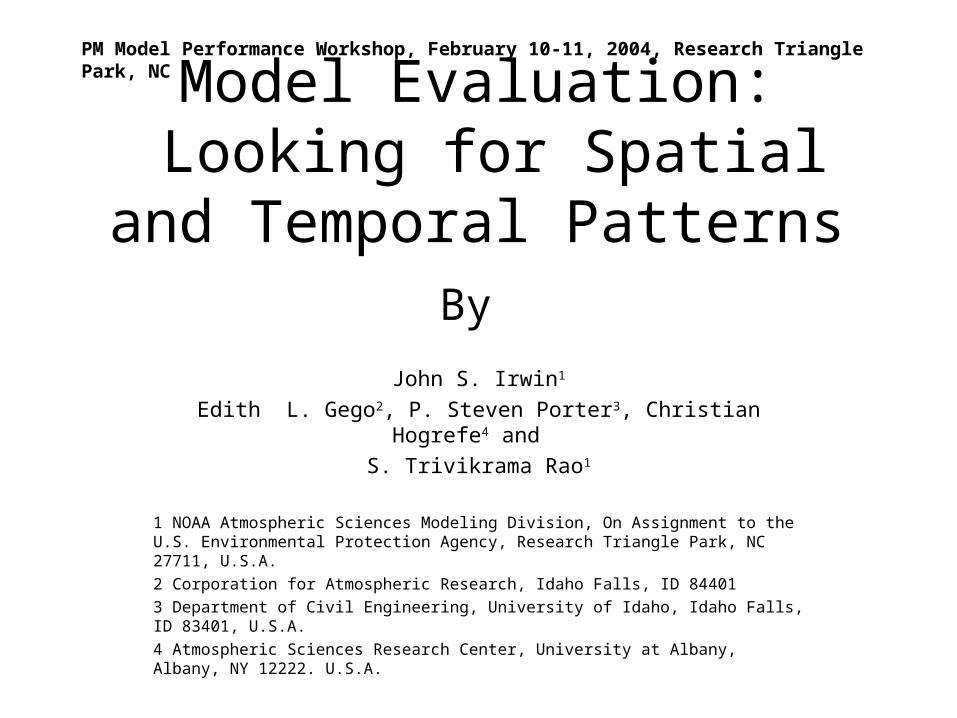
Model Evaluation: Looking for Spatial and Temporal Patterns

By

John S. Irwin1

Edith L. Gego2, P. Steven Porter3, Christian Hogrefe4 and

S. Trivikrama Rao1

1 NOAA Atmospheric Sciences Modeling Division, On Assignment to the U.S. Environmental Protection Agency, Research Triangle Park, NC 27711, U.S.A.

2 Corporation for Atmospheric Research, Idaho Falls, ID 84401

3 Department of Civil Engineering, University of Idaho, Idaho Falls, ID 83401, U.S.A.

4 Atmospheric Sciences Research Center, University at Albany, Albany, NY 12222. U.S.A.

PM Model Performance Workshop, February 10-11, 2004, Research Triangle Park, NC

a) b)

c)

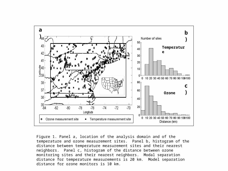
Figure 1. Panel a, location of the analysis domain and of the temperature and ozone measurement sites. Panel b, histogram of the distance between temperature measurement sites and their nearest neighbors. Panel c, histogram of the distance between ozone monitoring sites and their nearest neighbors. Modal separation distance for temperature measurements is 20 km. Model separation distance for ozone monitors is 10 km.

Temperature

Ozone

a)

b)

c)

Temper. (o C.)

Difference between the 12 km and the 4 km predictions ( 0C)

Frac

tion

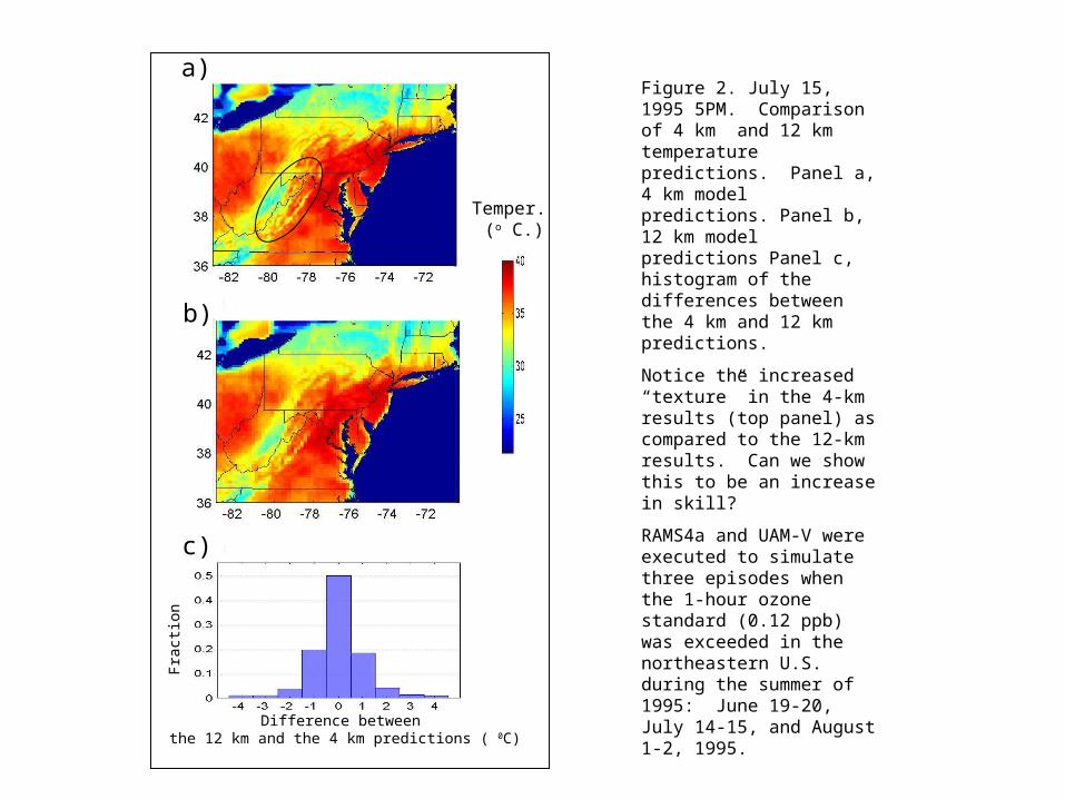
Figure 2. July 15, 1995 5PM. Comparison of 4 km and 12 km temperature predictions. Panel a, 4 km model predictions. Panel b, 12 km model predictions Panel c, histogram of the differences between the 4 km and 12 km predictions.

Notice the increased “texture” in the 4-km results (top panel) as compared to the 12-km results. Can we show this to be an increase in skill?

RAMS4a and UAM-V were executed to simulate three episodes when the 1-hour ozone standard (0.12 ppb) was exceeded in the northeastern U.S. during the summer of 1995: June 19-20, July 14-15, and August 1-2, 1995.

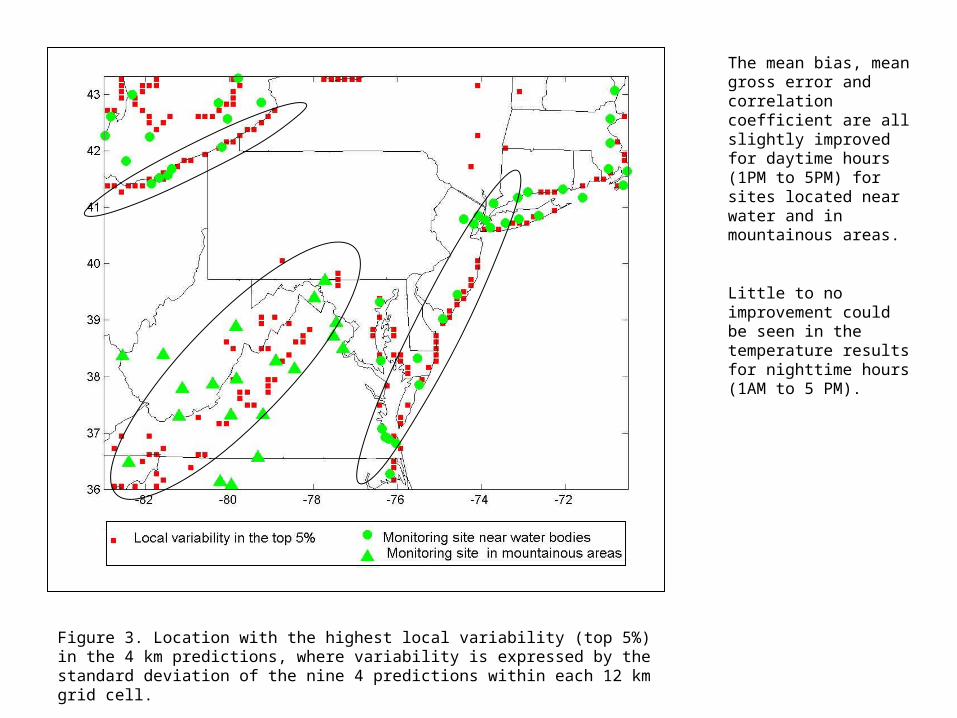
Figure 3. Location with the highest local variability (top 5%) in the 4 km predictions, where variability is expressed by the standard deviation of the nine 4 predictions within each 12 km grid cell.

The mean bias, mean gross error and correlation coefficient are all slightly improved for daytime hours (1PM to 5PM) for sites located near water and in mountainous areas.

Little to no improvement could be seen in the temperature results for nighttime hours (1AM to 5 PM).

Ozone (ppb)

a)

b)

c)

Difference between the 12 km and the 4 km predictions (ppb)

Frac

tion

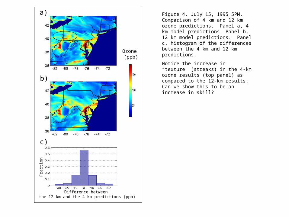
Figure 4. July 15, 1995 5PM. Comparison of 4 km and 12 km ozone predictions. Panel a, 4 km model predictions. Panel b, 12 km model predictions. Panel c, histogram of the differences between the 4 km and 12 km predictions.

Notice the increase in “texture” (streaks) in the 4-km ozone results (top panel) as compared to the 12-km results. Can we show this to be an increase in skill?

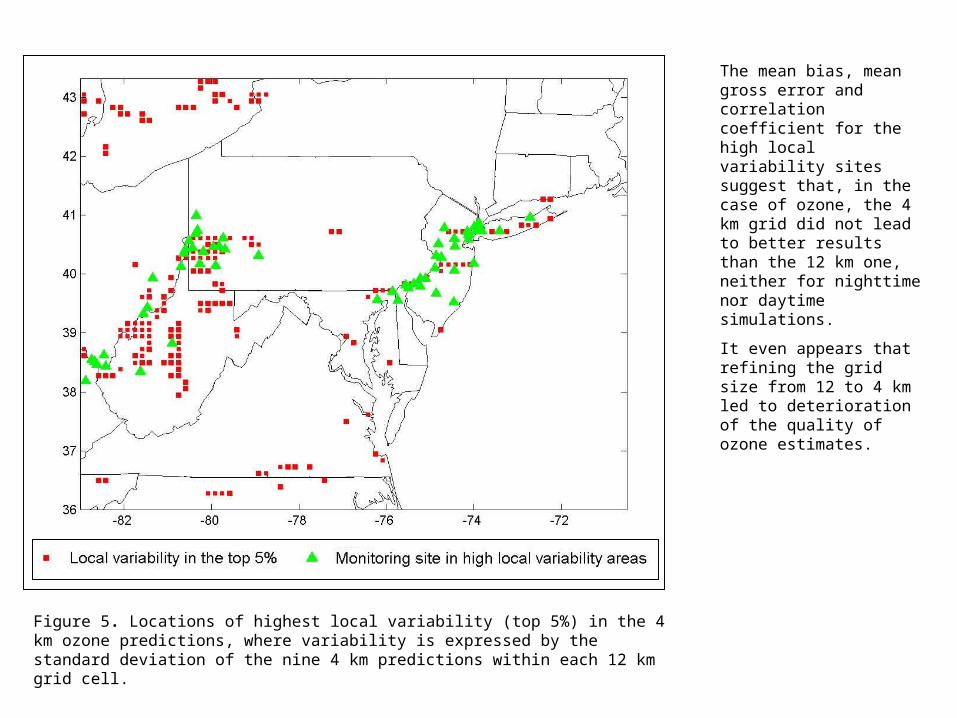
Figure 5. Locations of highest local variability (top 5%) in the 4 km ozone predictions, where variability is expressed by the standard deviation of the nine 4 km predictions within each 12 km grid cell.

The mean bias, mean gross error and correlation coefficient for the high local variability sites suggest that, in the case of ozone, the 4 km grid did not lead to better results than the 12 km one, neither for nighttime nor daytime simulations.

It even appears that refining the grid size from 12 to 4 km led to deterioration of the quality of ozone estimates.

c) d)

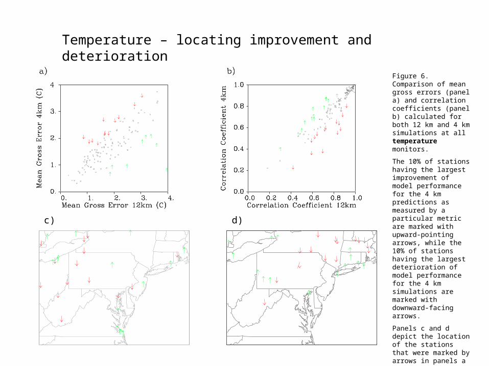
Figure 6. Comparison of mean gross errors (panel a) and correlation coefficients (panel b) calculated for both 12 km and 4 km simulations at all temperature monitors.

The 10% of stations having the largest improvement of model performance for the 4 km predictions as measured by a particular metric are marked with upward-pointing arrows, while the 10% of stations having the largest deterioration of model performance for the 4 km simulations are marked with downward-facing arrows.

Panels c and d depict the location of the stations that were marked by arrows in panels a and b, respectively.

Improvements look to be for grids near water.

Temperature – locating improvement and deterioration

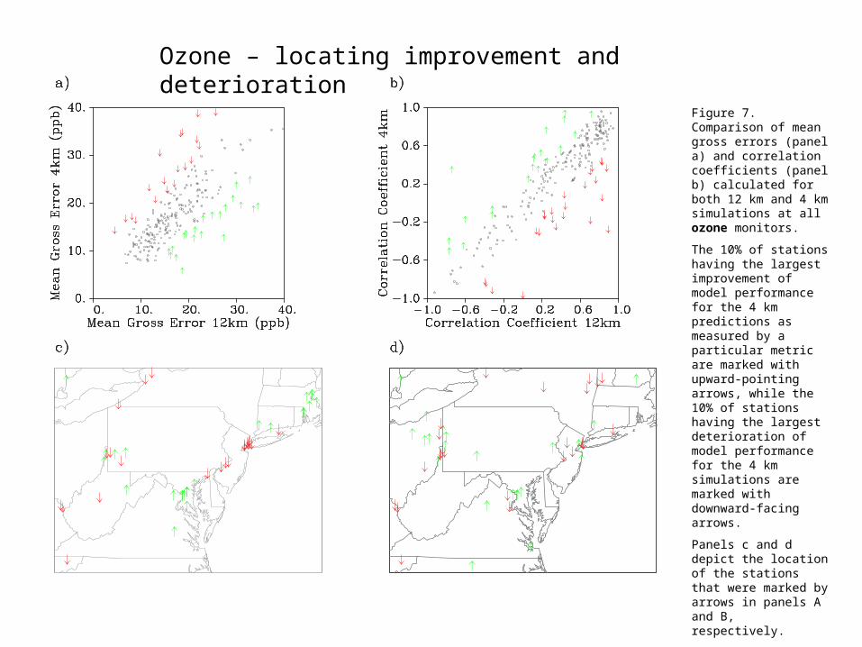
Figure 7. Comparison of mean gross errors (panel a) and correlation coefficients (panel b) calculated for both 12 km and 4 km simulations at all ozone monitors.

The 10% of stations having the largest improvement of model performance for the 4 km predictions as measured by a particular metric are marked with upward-pointing arrows, while the 10% of stations having the largest deterioration of model performance for the 4 km simulations are marked with downward-facing arrows.

Panels c and d depict the location of the stations that were marked by arrows in panels A and B, respectively.

It is difficult to see any obvious clustering or patterns.

Ozone – locating improvement and deterioration

1999 2000 2001 1999 2000 2001

Sulfateg/m3 CASTNet IMPROVE

Sulfateg/m3

A

B

C

A

B

C

1999 2000 2001 1999 2000 2001

Nitrateg/m3 CASTNet IMPROVE

Nitrateg/m3

A

B

C

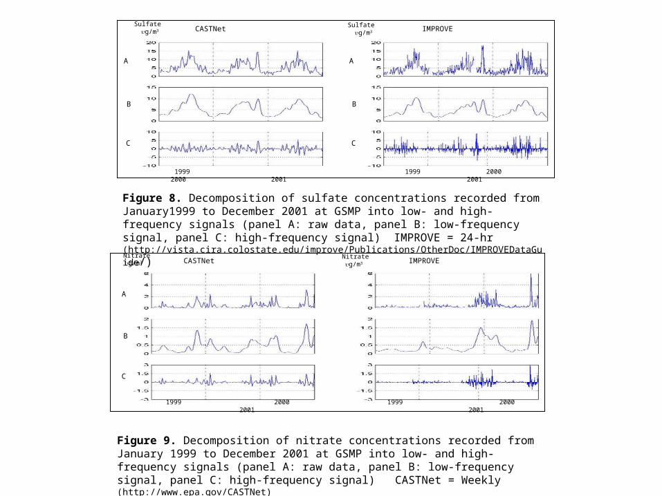
Figure 8. Decomposition of sulfate concentrations recorded from January1999 to December 2001 at GSMP into low- and high-frequency signals (panel A: raw data, panel B: low-frequency signal, panel C: high-frequency signal) IMPROVE = 24-hr (http://vista.cira.colostate.edu/improve/Publications/OtherDoc/IMPROVEDataGuide/)

Figure 9. Decomposition of nitrate concentrations recorded from January 1999 to December 2001 at GSMP into low- and high-frequency signals (panel A: raw data, panel B: low-frequency signal, panel C: high-frequency signal) CASTNet = Weekly (http://www.epa.gov/CASTNet)

Sulfate

Ammonium

Nitrate

A BConcentration

(ug/m3)

Castnet Improve STN

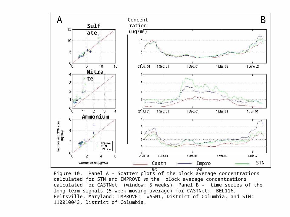
Figure 10. Panel A - Scatter plots of the block average concentrations calculated for STN and IMPROVE vs the block average concentrations calculated for CASTNet (window: 5 weeks), Panel B - time series of the long-term signals (5-week moving average) for CASTNet: BEL116, Beltsville, Maryland; IMPROVE: WASN1, District of Columbia, and STN: 110010043, District of Columbia.

CASTNet IMPROVE STN

Mid-Atlantic States

Kentucky area

Southeastern States

CASTNet IMPROVE STN

Western Great Lakes States

New England States

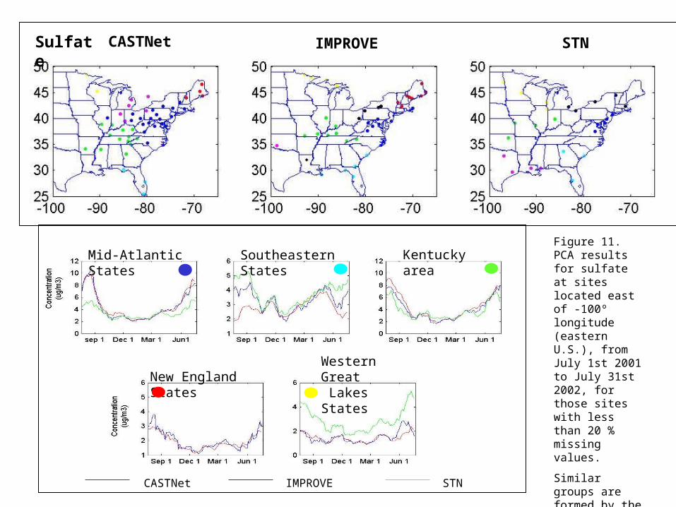
Figure 11. PCA results for sulfate at sites located east of -100º longitude (eastern U.S.), from July 1st 2001 to July 31st 2002, for those sites with less than 20 % missing values.

Similar groups are formed by the three networks, although some differences are evident in the time series within the groups.

Sulfate

CASTNet IMPROVE STN

Mid-Atlantic States Southeastern States

New England States Mid-West States

CASTNet IMPROVE STN

Kentucky area

Western Great Lakes States

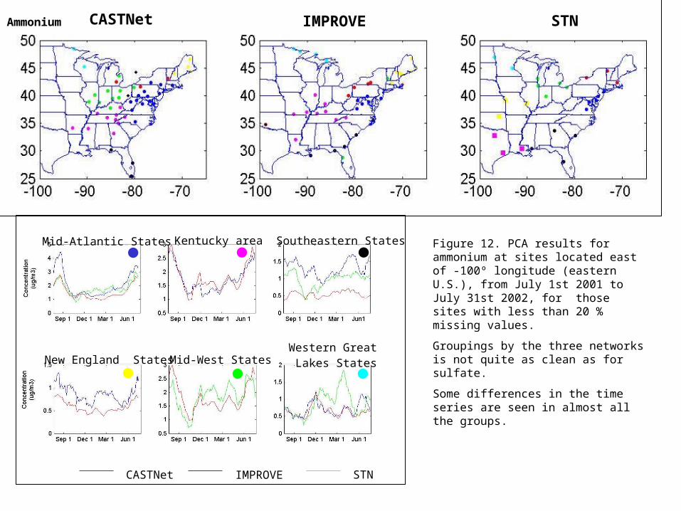
Figure 12. PCA results for ammonium at sites located east of -100º longitude (eastern U.S.), from July 1st 2001 to July 31st 2002, for those sites with less than 20 % missing values.

Groupings by the three networks is not quite as clean as for sulfate.

Some differences in the time series are seen in almost all the groups.

Ammonium

CASTNet IMPROVE STN

CASTNet IMPROVE STNSulfate

Nitrate

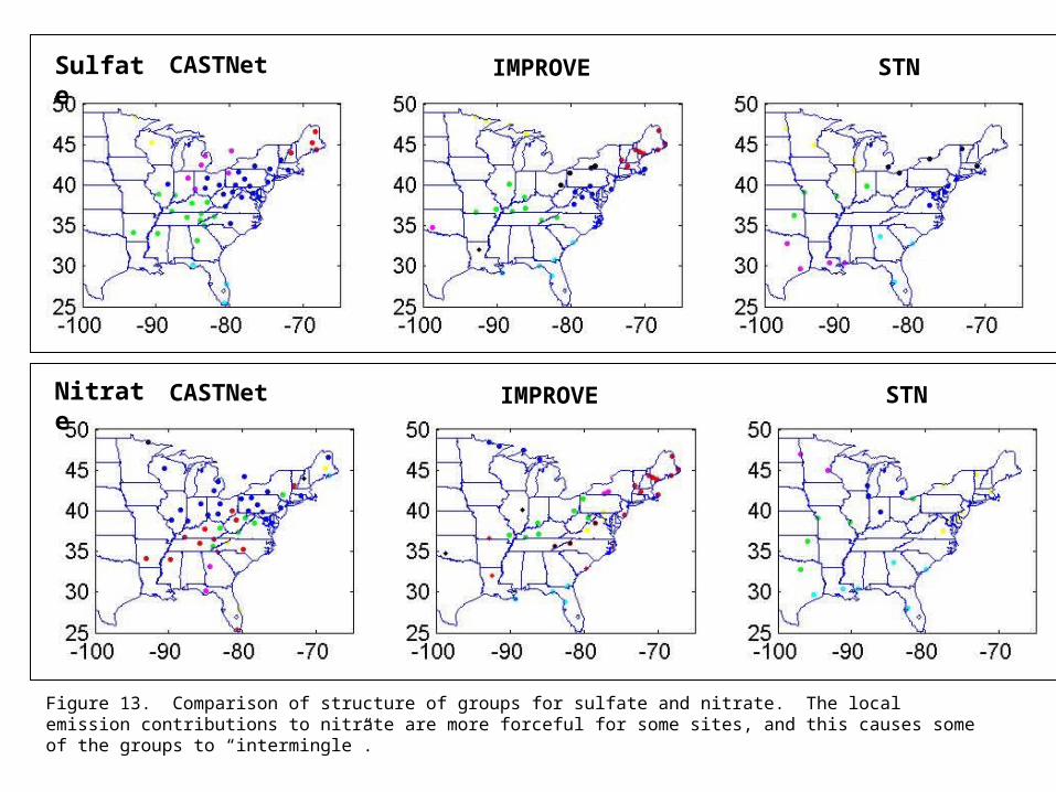
Figure 13. Comparison of structure of groups for sulfate and nitrate. The local emission contributions to nitrate are more forceful for some sites, and this causes some of the groups to “intermingle”.

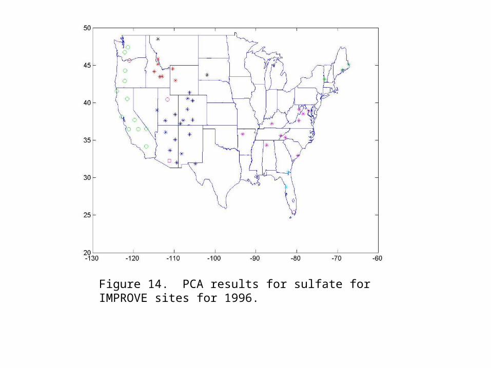
Figure 14. PCA results for sulfate for IMPROVE sites for 1996.

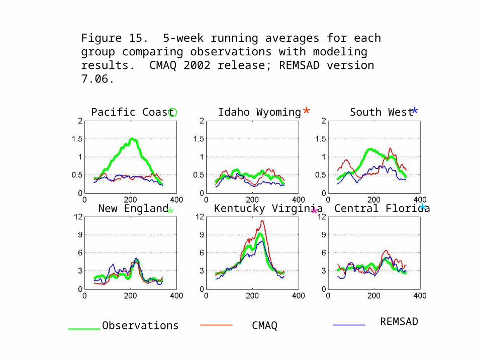
Figure 15. 5-week running averages for each group comparing observations with modeling results. CMAQ 2002 release; REMSAD version 7.06.

Pacific Coast Idaho Wyoming South West

New England Kentucky Virginia Central Florida

* *

* * *

Observations CMAQ REMSAD

6 0 1 2 0 1 8 0 2 4 0 3 0 0 3 6 0D a y N u m b e r

1x100

1x101

Su

lfat

e C

on

cen

trat

ion

O bservedC M AQR EM SAD

W ashington D .C . W ASH 1 -77.03330 East longitude 38.88330 North la titude

C M AQ N M SE = 0 .12 STD = 0 .0206 R EM SAD N M SE = 0 .07 STD = 0 .0133 t-Value = 1 .608

6 0 1 2 0 1 8 0 2 4 0 3 0 0 3 6 0D a y N u m b e r

1x10 - 1

1x100

Su

lfat

e C

on

cen

trat

ion

O bservedC M AQR EM SAD

B ryce C anyon BR C A1 -112.16670 East longitude 37.60000 North latitude

C M AQ N M SE = 0 .49 STD = 0 .0301 R EM SAD N M SE = 0 .50 STD = 0 .0126 t-Va lue = -0 .530

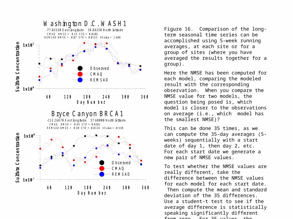
Figure 16. Comparison of the long-term seasonal time series can be accomplished using 5-week running averages, at each site or for a group of sites (where you have averaged the results together for a group).

Here the NMSE has been computed for each model, comparing the modeled result with the corresponding observation. When you compare the NMSE value for two models, the question being posed is, which model is closer to the observations on average (i.e., which model has the smallest NMSE)?

This can be done 35 times, as we can compute the 35-day averages (5-weeks) sequentially with a start date of day 1, then day 2, etc. For each start date we generate a new pair of NMSE values.

To test whether the NMSE values are really different, take the difference between the NMSE values for each model for each start date. Then compute the mean and standard deviation of the 35 differences. Use a student-t test to see if the average difference is statistically speaking significantly different from zero. For 35 values, the computed t-test (Mean/SD) must be greater than 1.96 to have 95% confidence that the mean of the 35 differences is different from zero. ASTM Standard Guide D 6589.

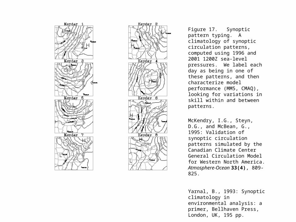
Figure 17. Synoptic pattern typing. A climatology of synoptic circulation patterns, computed using 1996 and 2001 1200Z sea-level pressures. We label each day as being in one of these patterns, and then characterize model performance (MM5, CMAQ), looking for variations in skill within and between patterns.

McKendry, I.G., Steyn, D.G., and McBean, G., 1995: Validation of synoptic circulation patterns simulated by the Canadian Climate Center General Circulation Model for Western North America. Atmosphere-Ocean 33(4), 809-825.

Yarnal, B., 1993: Synoptic climatology in environmental analysis: a primer, Bellhaven Press, London, UK, 195 pp.

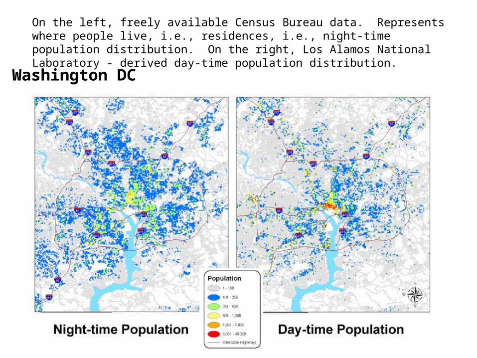
Washington DC

On the left, freely available Census Bureau data. Represents where people live, i.e., residences, i.e., night-time population distribution. On the right, Los Alamos National Laboratory - derived day-time population distribution.

The presentation is broken into three parts.

1) Available monitors are too far apart for spatial interpolation for assessment of whether fine-scale photochemical models are adding valid information (Is the increased "texture" seen in such simulations an increase in model skill?), so we attempted to assess performance by other means (see Figures 2-7, Tables 1 and 2) - we concluded that for temperature, going from 12km to 4km may have improved the temperature estimates ever so slightly along the coastlines, but we could not confirm an increase in skill for the ozone predictions in going from 12km to 4km.

2) We compared measurements from the three aerosol networks for sulfate, nitrate and ammonium. PCA analysis and comparison of long-term temporal time series suggest that the three networks have similar spatial patterns and similar (long-term) temporal patterns (within the subregions) for sulfate and ammonium; nitrate measurements appear somewhat different and will require further work to fully understand.

3) We used our understanding of PCA on sulfate to see if we could devise a way to assess model performance. It appears that when we look and the long-term temporal patterns predicted and observed in the PCA subregions, we can detect where the model is performing well and where it is failing (e.g., failure of sulfate predictions over most of western states, and especially along west coast). We plan to explore how we can adapt this evaluation method for ammonium and nitrate. We plan to extend this work to assess model performance within the subregions based on the synoptic situation We provide an example of how differences in model performance in simulating the 5-week average sulfate concentrations can be objectively determined.

The last slide in the presentation is there (if I have time) to alert people to start thinking of population as a function of time of day, which will possibly affect emission inventories and most definitely will affect exposure assessments. This slide is from a presentation I heard up in DC as part of the homeland defense meetings I am going to. One of the other "comments" mentioned at this meeting was that it was estimated that "urban" as a land-use description was likely underestimated in the US by about 50%.....food for thought....