Embed Size (px)
Citation preview

Simulation, Analysis, andModel Order Reduction for
Dynamic Power Network Models
A master thesis submitted by
Frances Weiß
to theFaculty of Mathematics
Otto-von-Guericke University Magdeburgin partial fulfillement of the requirements
for the degree of
Master of Science
in
Mathematics
Dr. Sara GrundelAdvisor and 1st reviewer,Max Planck Institute for Dynamics of Complex Technical Systems, Magdeburg
Jun.-Prof. Dr. Jan Heiland2nd reviewer,Otto-von-Guericke University MagdeburgMax Planck Institute for Dynamics of Complex Technical Systems, Magdeburg
Dr. Manuel BaumannCo-advisor,Max Planck Institute for Dynamics of Complex Technical Systems, Magdeburg
Submitted: August 30, 2019


AcknowledgmentsFirst of all, I would like to thank my supervisor, Sara Grundel, and my co-advisor,Manuel Baumann, for their support, time, andpatience. With their guidance, I learned alot ofmeans and tricks to overcomemathematical challenges, and I extendedmy skill setgreatly during the work on this thesis. I would also like to thank Jan Heiland for agree-ing to be my second reviewer. There are many other people at the Max-Planck-InstituteMagdeburg who deserve credit for giving useful input. Especially Martin Köhler spenta lot of time trying to get me server and MATLAB access.
A thank you to the team at the Very Large Business Applications Lab, too, for beingsuch endearing colleagues. They provided me with with a place to work and even aplace to sleep when I needed it.
Finally, I want to express my deepest gratitude to my entire family. Without myextraordinary wife, her love, her encouragement and her belief in me, I would neverhave been able to accomplish this. Ein unendlich großer Dank geht an meine phänom-enalen Eltern. Ihre Liebe, Geduld und Unterstützung haben mir so viel Kraft und Aus-dauer geschenkt – unter anderem. Es gibt keine Worte für all das, was sie mir gegebenhaben. Ich danke auch meiner Schwester, meinem Bruder, meinem Schwager, meinerSchwägerin, meinen Neffen, meiner Nichte, meiner Omi und Tante für ablenkendeGespräche und Besuche, und Verständnis für verpasste Familienfeiern. Ich habe euchso lieb!
Danke. Thank you.
iii

iv

List of Tables
2.1 Known and Unknown Parameter Values . . . . . . . . . . . . . . . . . . . 12
4.1 Coupled Oscillator Model Parameters . . . . . . . . . . . . . . . . . . . . 494.2 Attributes of MOR Methods . . . . . . . . . . . . . . . . . . . . . . . . . . 61
5.1 Model-Independent MOR Parameters for case57 . . . . . . . . . . . . . . 655.2 Model-Dependent MOR Parameters for case57 . . . . . . . . . . . . . . . 66
v

vi

List of Figures
2.1 Power Network Modeling Process of the EN Model . . . . . . . . . . . . 162.2 Power Network Modeling Process of the SMModel . . . . . . . . . . . . 19
3.1 Graphical Depiction of Model Order Reduction (MOR) Process for Lin-ear Systems . . . . . . . . . . . . . . . . . . . . . . . . . . . . . . . . . . . 25
3.2 Graphical Depiction of MOR Process for Quadratic Systems . . . . . . . 35
4.1 Sparsity Pattern of A (EffectiveNetwork (EN)model, 3-generator/9-nodessystem, nco = 3) . . . . . . . . . . . . . . . . . . . . . . . . . . . . . . . . . 53
4.2 Sparsity Pattern of H (EN model, 3-generator/9-nodes system, nco = 3) 564.3 Sparsity pattern of A (EN model, 3-generator/9-nodes system, nco = 3) . 58
5.1 IEEE case57 power flow system . . . . . . . . . . . . . . . . . . . . . . . . 645.2 Output of Full-Order Model for case57 . . . . . . . . . . . . . . . . . . . . 645.3 Output of BT3 . . . . . . . . . . . . . . . . . . . . . . . . . . . . . . . . . . 695.4 Output of BT3 for 10s Interval . . . . . . . . . . . . . . . . . . . . . . . . . 705.5 Output of POD for 10s Interval . . . . . . . . . . . . . . . . . . . . . . . . 725.6 L∞ Output Error for BT1, BT3, BT5, and POD . . . . . . . . . . . . . . . . 735.7 L∞ Output Error for BT1, BT3, BT5, and POD for 10s Interval . . . . . . . 745.8 L∞ Pythagorean Trigonometric Identity (PTI) Error for BT1, BT3, BT5,
and POD . . . . . . . . . . . . . . . . . . . . . . . . . . . . . . . . . . . . . 765.9 Hankel singular values (SVs), and SVs of Gramians P ,Q . . . . . . . . . 795.10 Singular Values of POD Snapshot Matrices for Lifted Quadratic and Un-
lifted Nonlinear System . . . . . . . . . . . . . . . . . . . . . . . . . . . . 805.11 L∞ Output Error for (δ0, C) pairs of Initial Values and Output Matrices . 815.12 Impact of Different Aα on L∞ Output Error . . . . . . . . . . . . . . . . . 82
B.1 Sparsity Pattern of H(2) (EN model, 3-generator/9-nodes system, nco = 3) 97
vii

viii

List of Algorithms
2.1 Kron Reduction (cf. [BV00]) . . . . . . . . . . . . . . . . . . . . . . . . . . 14
3.1 Lyapunov-Cholesky Routine . . . . . . . . . . . . . . . . . . . . . . . . . . 453.2 Iterative Scheme to Compute Truncated Gramian PT . . . . . . . . . . . . 463.3 Balanced Truncation Algorithm for Quadratic Systems . . . . . . . . . . . 473.4 Proper Orthogonal Decomposition for Quadratic Systems . . . . . . . . . 48
C.1 Iterative Scheme to Compute Truncated Gramian QT . . . . . . . . . . . . 101
ix

x

Contents
Acknowledgments iii
List of Tables v
List of Figures vii
List of Algorithms ix
Glossary and Acronyms xiii
1 Introduction 1
2 Dynamic Power Network Modeling 52.1 Basic Concepts of Power System Analysis . . . . . . . . . . . . . . . . . . 62.2 The Basic Power Network Model for Generator Nodes . . . . . . . . . . . 82.3 The Basic Power Network Model for Load Nodes . . . . . . . . . . . . . . 13
2.3.1 Effective Network Model . . . . . . . . . . . . . . . . . . . . . . . 152.3.2 Synchronous Motor Model . . . . . . . . . . . . . . . . . . . . . . 182.3.3 Model-Dependent Parameters: Characterization and Comparison 20
3 Model Order Reduction Methods for Dynamic Systems 233.1 Model Order Reduction . . . . . . . . . . . . . . . . . . . . . . . . . . . . 233.2 Balanced Truncation for (Linear) Dynamic Models . . . . . . . . . . . . . 273.3 Balanced Truncation for (Quadratic) Dynamic Models . . . . . . . . . . 333.4 Proper Orthogonal Decomposition . . . . . . . . . . . . . . . . . . . . . . 47
4 Mathematical Modeling 494.1 Transformation to Nonlinear Dynamic 1st-Order ODE System . . . . . . 504.2 Transformation to Quadratic Dynamic ODE System . . . . . . . . . . . . 50
4.2.1 Quadratic Dynamic ODE System - Equation version . . . . . . . . 504.2.2 Quadratic Dynamic ODE System - Matrix version . . . . . . . . . 52
4.3 Nonzero Initial Values . . . . . . . . . . . . . . . . . . . . . . . . . . . . . 574.4 Application of MOR to the Quadratic Dynamic Power Network System . 59
xi

5 Numerical Experiments for a Power Network Test Case 635.1 Test Setup and Parameters . . . . . . . . . . . . . . . . . . . . . . . . . . . 635.2 Proof-of-Concept: Output-over-Time Behavior . . . . . . . . . . . . . . . 685.3 Cross-Method-Comparison of Output Error . . . . . . . . . . . . . . . . . 735.4 Cross-Method-Comparison of Pythagorean Trigonometric Identity Error 765.5 Evolution of the Singular Values . . . . . . . . . . . . . . . . . . . . . . . 785.6 Influence of Initial Value & Output Matrix on Output Error . . . . . . . . 805.7 Influence of α-Shift on Output Error . . . . . . . . . . . . . . . . . . . . . 81
6 Summary and Conclusion 85
A More on Gramians, Stability and Energy Functionals for Balanced Truncation 87
B Multi-Linear Algebra Operations 95
C Notes on Codes 99
Bibliography 100
xii

Glossary and Acronyms
Glossary
A matrix describing linear part of quadratic systemα shift parameter to stabilize the A matrixB input matrix of quadratic systemC output matrix of quadratic systemc cosine values of angles: c = cos(δ)
coupled oscillator representation PN represented as a system of coupled oscillatorswith arbitrary coupling structure; exact coupling struc-ture defined by power network (PN) models, , seeoscillator
D damping coefficient characterizing the oscillatorsδ phase angle relating to the internal voltage magni-
tude |E| at an internal nodeelectric circuit representation PN represented as a system of electric components
characterized by electric power lawsE voltage at an internal node with magnitude |E|ε absolute L∞ errorF one of the parameters determining the inherent fre-
quencyg used as a super- or subscript indicating values con-
cerning generator nodesγ phase shift involved in oscillator couplingγc cosine values of phase shifts: γc = cos(γ)
γs sine values of phase shifts: γs = sin(γ)
generator node an element in the PN system which transforms me-chanical into electric power
H matrix describing quadratic part of quadratic systemi imaginary unitinternal node an element in the PN system between the constant-
magnitude voltage source (with time-dependent phase)
xiii

and the transient reactance x′rI electric current, the flow of electric chargeJ inertia coefficient characterizing the oscillatorsK strength of dynamic coupling between two oscilla-
tors` used as a super- or subscript indicating values con-
cerning load nodesλ eigenvaluelink an electric connection between two nodes, either a
transmission line or a transformerload node an element in the PN system which consumes elec-
tric powern number of nodes in the physical representation of
the PNnco number of nodes in the coupled oscillator represen-
tation of the PN, equals the number of equations inthe ODE system after application of one of the PNmodels
nec number of nodes in the electric circuit representationof the PN
ng number of generator nodes in the PNn` number of load nodes in the PNnmin singular valuenode an element in the PN system at which power is in-
jected by a generator or extracted by consumers or abranchingpoint throughwhichpower is redistributed
nρ number of equations in the reduced-order modelν number ofVolterra kernels in the computation ofP ,Qϕ? inherent frequency of an oscillator in a PN systemϕR reference frequency for a PN systemoscillator can represent either a generator or a load nodeP active power in the power flow equationP reachability Gramian matrixPe electric power consumed by the nongenerator com-
ponents of the networkφ phase angle relating to the complex voltage magni-
tude |V|physical representation PN represented with the actual hardware compo-
nents used to built the network
xiv

Pm net mechanical power input to the generator rotorpower network generic term for different types of power grid repre-
sentationsQ observability Gramian matrixQ reactive power in the power flow equationreference node an element in the PN system to account for the un-
known power losses in the systemR Cholesky factor of the reachability Gramian Pnρ reduction order of the MORs sine values of angles: s = sin(δ)
S Cholesky factor of the observability Gramian Qσ singular valuet used as a superscript indicating values concerning
terminal nodesterminal node an element in the PN system allowing the circuit to
interconnectwith its environment and connecting thegenerator to the rest of the network
ϑ phase angle of the PN model’s admittance matrixtransmission line an electric coupling between two nodes, see linku input vector of quadratic systemV projectionmatrix of theMORcontaining the left-singular
vectorsV complex voltage with magnitude |V|W projection matrix of the MOR containing the right-
singular vectorsx state vector with phase angles, their first derivatives,
their sin and cos substitutions: x = [δ, ω, s, c]∗
x′r transient reactance, opposition to a change in electriccurrent effective after the damper winding currentshave diminished
y output vector of quadratic systemY admittance matrixY complex admittance
Acronyms
BT Balanced TruncationCO coupled oscillator, see also glossary entryEC electric circuit, see also glossary entry
xv

EN Effective NetworkEV eigenvalueEVD Eigenvalue DecompositionFOM full-order modelIVP initial value problemLHS left hand sideMOR Model Order ReductionODE Ordinary Differential EquationPN power network, see also glossary entryPOD Proper Orthogonal DecompositionPTI Pythagorean Trigonometric IdentityRHS right hand sideROM reduced-order modelSM Synchronous MotorSPD symmetric positive definiteSV singular valueSVD Singular Value Decomposition
Symbols
I identity matrix⊗ Kronecker product1 matrix of all ones? value of a state variable for a power flow solutionM∗ transpose if M ∈ Rn×k, complex conjugate transpose
if M ∈ Cn×k,0 matrix of all zeros
xvi

CHAPTER 1
Introduction
Motivation
Dynamic systems are used in a multitude of applications. A lot of them have an in-creasingly complex structure, e.g., control problems like heating and cooling processesor chemical reactions, or prediction problems like weather forecasts or biological pro-cesses. The numerical simulation of these problems attempts to predict or control thesystem behavior in order to test features or ascertain its conduct over time [Ant05;AS01].
In this thesis, we engage in a particular aspect of PNmodeling as an example simula-tion problem, namely, the synchronization stability of power generators. If a single generatorruns at a different frequency, the PN will fail to operate properly. A capable PN modelmust therefore incorporate the dynamics between coupled power generators as part ofthe network structure. Due to the advent of better computational capabilities and dataprocessingmethods researchers have been enabled to study large-scale features like thenetwork structure.
Reasons for asynchronicity might be fluctuations in power demand or the malfunc-tion of system components [NM15a]. The implementation of smart-grids and the in-sertion of less reliable renewable energy sources, e.g., wind and solar power, will makethe networks even more vulnerable to instability [DB12]. Due to these developments,the overall importance of synchronization stability, and a research gap regarding theinfluence of the network structure on the interconnected system dynamics have madethis an area of active research in recent years [DB12; NM15a]. [NM15a] compare threeleadingmodels in their paper on power network synchronization, two ofwhich are con-sidered in this thesis. They are all based on a common design, representing the PN’sstructure as an interlinked 2nd-order system of Ordinary Differential Equations (ODEs)with nonlinear dynamics. In their paper, [NM15a] derive the model-dependent param-eters which are necessary to find a solution to the ODE systems. However, they do notactually solve these systems. This is the first motivation of this thesis.
Faithfullymodeling such large-scale systems requires a considerable number of statevariables. The model is therefore often highly complex and its full simulation faces anumber of difficulties: Its complexity might be too large to meet storage limitations.
1

CHAPTER 1. Introduction
Also, computation resultsmust be produced in reasonable time. Using large-scalemod-els might therefore be infeasible due to limited computational speed. Furthermore, ac-curacy suffers from the finite precision representation of numbers in computers and theill-conditioning of large-scale systems [Ant05; AS01]. Although these problems haveindeed been mitigated by the rise of computational capabilities in the last years, high-complexity models of dimension up to 106 present a challenge, nonetheless.
MOR offers to overcome this dilemma by providing a reduced-order model (ROM)of the original system. AROMmustmanage the balancing act of being of low-dimensionby downsizing the number of state variables on the one hand, while simultaneously ap-proximating the full-order model (FOM)’s input-output-behavior with an acceptableerror and maintain significant system properties on the other hand [BG17].
While MOR theory and methods have been thoroughly studied and used in prac-tice regarding linear systems, the development and adaptation of MOR techniques inthe nonlinear context is a work in progress. In general, nonlinear MOR presents chal-lenges which make it more difficult than reducing linear systems. One of the problemsis the possibly costly computation, even after the reduction. Solving the nonlinear ROMcan be just as costly as the original system, rendering the MOR ineffective. Another is-sue is the unpredictable behavior of the reduced system. A priory, it is often unclearwhich (global) properties the ROM will retain from the FOM. Also, nonlinear systemsdo not provide a canonical form for the ROM. This makes it hard to find an adequaterepresentation and construct useful algorithms [Gu11].
To remedy these challenges, several approaches have been taken. One is to linearizethe nonlinear system around an expansion point and subsequently apply linear MOR.This represents the systemdynamicswell in the vicinity of the expansion point, but failsas the distance grows larger. For this reason, nonlinear dynamics should be reflectedin the MOR process. The Proper Orthogonal Decomposition (POD) method in its var-ious incarnations is a popular example which has been successfully applied to generalnonlinear systems [BG17; KW19; Pin08; RP03; Vol13]. For several years, there has alsobeen a focus on extending techniques originally designed for linear systems to nonlin-ear systems with a specific structure. Especially bilinear systems have received muchattention, because a lot of biological, physical and physiological processes can be mod-eled in the form of such systems [BBF14; BGR17; BPK71; Fla12; VG18]. More recently,quadratic-bilinear systems have been studied with regard to MOR. Lifting a nonlinearto a quadratic-bilinear system by adding auxiliary variables to the state vector mightnot result in a unique representation, but it is an exact process, i.e., there is no addedapproximation error [BBF14; BG17; Gu11; KW19].
In contrast, transforming nonlinear systems to give them a quadratic structure hasbeen largely disregarded in MOR research so far [BBF14; Che99]. The second motiva-tion of this thesis is thus to lift the nonlinear PN ODE systems to quadratic form, and
2

explore the application of the Balanced Truncation (BT) MOR method to these trans-formed systems. The method is adapted to the quadratic context beforehand, based onthe work by [BG17].
The overall goal of this thesis is to examine the performance of BT applied to thequadratic version of the PN ODE systems. To that end, we solve the systems for theFOM and ROM and vary different reduction parameters to study their influence.
Outline
We approximate our overall goal by first exploring our twomainmotivations separatelyin stand-alone chapters.
We begin Chapter 2 by introducing some concepts and terminology of power systemanalysis. Building on this basis, we derive the dynamic power network models. Thisincludes a characterization and comparison of themodel-dependent parameters. At theend, we have two similar nonlinear 2nd-order ODE systems of different sizes.
In Chapter 3, we present the problem setup and idea of MOR in general, and BTin particular, in their linear and nonlinear setting. We introduce the key concepts ofreachability and observability, the respective Gramians and how they facilitate the ac-tual process of balancing and truncating, highlighting distinct features of the quadraticcase. In addition, we establish the basics of Proper Orthogonal Decomposition (POD),a method we use to compare the performance of quadratic BT.
While Chapters 2 and 3 are independent of each other, we link their topics in Chap-ter 4. Since the derived PN models lack structure, we bring them into the appropriatequadratic form in a multi-step process. We also look at the necessary assumptions forthe application of BT and take care of their satisfaction.
In Chapter 5, we consider a PN test case to evaluate the performance of quadratic BT.We apply the method to the two PN models generated from the test case and compareit to the POD method.
In the last chapter, Chapter 6, we conclude with summarizing and assessing thefindings.
3

CHAPTER 1. Introduction
4

CHAPTER 2
Dynamic Power Network Modeling
As mentioned in the introduction, a power network can only operate if all of its gen-erators run at the same frequency. The coupling dynamics between the generators de-termine their state and therefore the synchronization stability of the system. In conse-quence, a good networkmodel must properly describe the coupling dynamics of powergenerators. There are various ways to do this, here we focus on two leadingmodels: theEN model and the Synchronous Motor (SM) model.1 These models express a PN sys-tem containing generator and load nodes as a network of coupled phase oscillators.Therefore, we refer to the EN and SM models as types of coupled oscillator (CO) models.
The state of each PN node i is characterized by δi, its phase angle, and δi, its fre-quency [NM15a] or velocity [WT12]. With δi = δi(t) and i = 1, . . . , nco, the couplingdynamics between oscillators is described by a system of Ordinary Differential Equa-tions (ODEs), the so-called swing equations:
2Ji
ϕRδi +
Di
ϕRδi = Fi − ∑
j=1, j 6=iKij sin(δi − δj − γij), (2.1)
where the inertia J and damping D constants as well as the reference frequency ϕR
are model-independent coefficients determined by the physical structure of the system.The parameters F, K and γ, on the other hand, dependent on the modeling of the sys-tem’s nodes. While [NM15a] provide the derivation and a comparison of these model-dependent quantities, they do not solve the PN ODE system (2.1). This is one of ourmain objectives.
The purpose of this chapter is to retrace [NM15a]’s derivation of the parametersF, K, and γ, which are necessary to solve the equations in the ODE system (2.1) foreach generator and load node. These two types of nodes differ in their modeling, how-ever. While power generation can be regulated and is predictable to a certain extent,power consumption is affected by a number of different, time-dependent factors likethe load type, size and quantity of nodes as well as human activity. The two COmodelsvary mostly in their description of load nodes, and contingent on this, in the number
1In their paper, [NM15a] also discuss a third option, the Structure-Preserving model. It representsloads as first- and generators as second-order ODEs. Because it deviates in its derivation and structurefrom the other two models, it is disregarded in this work.
5

CHAPTER 2. Dynamic Power Network Modeling
of equations nco [NM15a]. We characterize the model-dependent parameters in Sec-tion 2.3.3. First, we introduce some power systems terminology and notation in thefollowing Section 2.1, which we use in the context of power network modeling. Then,we address generator node modeling in Section 2.2, before we focus on the load nodesin Section 2.3.
2.1 Basic Concepts of Power System Analysis
A power network is a system consisting of a number of nodes and links, operating todistribute power from generators to consumers. Power network is the generic term fordifferent types of power grid representations. First, there is the physical representa-tion, i.e., the actual hardware used to engineer the network. Second, the electric circuitrepresentation describes the network in terms of electric components and electric powerlaws. Third, the coupled oscillator representation characterizes the PN as a pure systemof coupled oscillators, where an oscillator can serve as either a generator or a load nodewith mathematical identical modeling [NM15a]. An oscillator is an electronic circuitwhich produces a periodic output, e.g., a sine or square wave [Sne].
A node is the generic term for a point in the network, where power is either injectedby a generator or extracted by a consumer or redistributed along branched off transmis-sion lines. We distinguish different kinds of nodes. The simplest distinction is betweengenerator nodes and load nodes. Both are elements in the power network system withthe former injecting power into the network by transforming mechanical into electricpower and the latter consuming said electric power. A terminal node allows the circuitto interconnect with its environment, and in our case specifically connects the genera-tor to the rest of the network [NM15a; Wil10]. An internal node is a point between theconstant-magnitude voltage source and the transient reactance x′r. [NM15a].
We also operate with two types of complex voltage: When we talk about the voltageat an internal node, we denote it by the internal voltage E. The symbol V indicates thegeneric complex voltage, but also the terminal voltage at a terminal node if explicitlymentioned.
The links are transmission lines and serve to electrically couple the nodes. Transmis-sion lines have complex-valued impedances. Admittances are the inverse of impedances.Due to this connection, the admittance matrix Y encodes the structure of the respec-tive network representation [NM15a]. The construction of an admittance matrix needsmuch less effort than the construction of an impedancematrix. Thematrix itself is oftensparse for large-scale PN, because each node typically has only a few links to neighbor-ing nodes. Therefore, it is a common approach in power system analysis to use equiva-lent admittances to express the parameters characterizing the transmission lines [GS94;NM15a]. An admittance matrix denoted by Y0, i.e., with an additional subscripted 0,represents the physical network structure [MMA+13; NM15a].
6

2.1. Basic Concepts of Power System Analysis
Reactance x is the imaginary part of the impedance and quantifies the opposition toa change in electric current I, the flow of electric charge [IL14]. The transient reactancex′r is the reactance effective after the damperwinding2 currents have diminished [GS94].
We encounter different concepts of power. The active power P makes up the realand the reactive power Q the imaginary parts of the complex power S, which adheresto the formulae
S = VI = P+ iQ = |V||I| cos(φ) + i|V||I| sin(φ), (2.2)
where V denotes the voltage, I the complex conjugate of the electric current, φ the phaseangle, and i is the imaginary unit [GS94; IL14; NM15a]. Furthermore, Pm is the netmechanical power input to the generator’s rotor. The electric power Pe is the requestedpower by the nongenerator components of the network [NM15a].
Another context-dependent term we use is the phase angle. While δ describes thephase angle at an internal node and always appears in conjunction with the internalvoltage magnitude |E|, φ represents the phase angle at a terminal or load node and con-sistently occurs with the voltage magnitude |V|. Which phase angle and voltage (mag-nitude) representation is used depends on the network component. The phase anglematrix ϑ is calculated from the respective CO model’s admittance matrix Y. The termγ denotes the phase angle shift in the oscillator coupling [NM15a].
Closely connected to angles are frequencies. The first derivative of a phase angle δ isthe node’s frequency δ. We make a distinction between the term ϕR, which is the refer-ence frequency for the PN system and an oscillator’s inherent frequency ϕ?, which is theequilibrium frequency of an oscillator in case there is no coupling to another oscillator[NM15a].
The oscillators are also characterized by the inertia J and damping D coefficients.Just like the reference frequency ϕR, the inertia and damping parameters are given bythe physical structure of the system [NM15a].
We refer to two important electric circuit laws. First, Kirchhoff’s current law says thatfor any node in a circuit the sum of currents which flow towards that node is identicalto the sum of currents which flow away from that node, i.e.,
∑jIj = 0, (2.3)
with I being the electric current. Second, we state Ohm’s law in the following way,
I =E− V
ix′r, (2.4)
where x′r is the transient reactance, and E and V stand for the internal and terminalvoltage, respectively. Using the admittance matrix Y, we can restate Ohm’s law in the
2The damper winding in a machine is responsible for the decrease of the mechanical oscillations of therotor approximately around synchronous speed.
7

CHAPTER 2. Dynamic Power Network Modeling
entire network as a matrix-vector product,
I = YV, (2.5)
with current vector I and voltage vector V, respectively [IL14; NM15a].We attempt to avoid confusion and use sans serif letters for those variables and pa-
rameters which primarily occur in the power systems context and serif or other specialfont types for those which primarily occur in the mathematical parts of this thesis. Forexample, the “P” for the active power P is not the same as the “P” for the matrix P .
In the context of power system analysis, we use bold letters whenever we mean ma-trices or vectors, e.g.,Y is the admittance matrix whereas Y is a scalar admittance value,and V is the voltage vector whereas V is a scalar voltage value. Whenever g, ` are usedas a super- or subscript they indicate values concerning generator or load nodes, re-spectively. A minuscule i used as a superscript, e.g., in gi, `i, refers to generator internaland load internal nodes, respectively, and a minuscule t used as a superscript, as in gt,refers to terminal nodes. The superscripted star ?marks the value of a state variable fora power flow solution, and a bar q above a variable q indicates the complex conjugate.
For quick reference, you can also find a concise explanation of these terms in theGlossary and Acronyms chapter, and a list of symbols, beginning on page xiii.
2.2 The Basic Power Network Model for Generator Nodes
The goal is to find computable expression of the model-dependent parameters F, K andγ in the dynamic system (2.1). To that end, we want to identify the quantities neces-sary to describe the state of a node. In this section, we focus on generator modeling andlook at two different representations of a generator to derive two important equations:the mechanical representation leads to the so-called swing equation and the electric circuitrepresentation introduces the classical model. On these grounds, we discover the char-acterizing quantities of a node’s state and how to compute them for generators at theend of this section.
The Swing Equation The Mechanical Representation of a Generator
Mechanically, a power generator often consists of a rotor (among other parts), i.e., arotating mass. Its motions are affected by a mechanical and an electric torque. Fromthese torques, the mechanical and electric power (Pm and Pe, respectively) working onthe rotor can be calculated by multiplication with the angular velocity of the rotor, ω
(frequently, the approximation ω ≈ ϕR is assumed). Usually, both types of torque arepositive, so that the mechanical torque corresponds to the generator’s power input, andthe electric torque corresponds to the power output or to the electric power demandedby the rest of the network. The mechanical power and torque are assumed to be con-stant, so the electric power and torque determine the rotation’s change in velocity, i.e., if
8

2.2. The Basic Power Network Model for Generator Nodes
the rotor is accelerated (Pm > Pe), decelerated (Pm < Pe), or steady (Pm = Pe) [GS94;NM15a]. This relative motion is expressed in the swing equation:
2JϕR
δ +DϕR
δ = Pm − Pe, (2.6)
the fundamental equation of motion for a generator. The inertia constant J is the ki-netic energy of the rotor divided by the rated power. The damping constant D is thecombined damping coefficient which - simply put - merges several quantities whichdecrease or impede the rotor’s oscillations. The angle δ is the rotor angle relative to aframe rotating at the reference frequency ϕR [NM15a]. The first and second deriva-tive of δ thus correspond to the velocity (or frequency) and acceleration of the rotor,respectively [GS94]. The systems (2.1) and (2.6) represent a dynamic system for δ.
The swing equation constitutes the linchpin of our further examination. The lefthand side (LHS) of the swing equation (2.6) is already in the form of the LHS of theODE system (2.1). The constants J, D and ϕR are determined by the underlying physicalpower network. The right hand side (RHS), in contrast, depends on time and themodelrepresentation which is employed. The classical model in the next subsection furnishesus with alternative expressions for Pm and Pe.
The Classical Model The Electric Circuit Representation of a Generator
Under realistic conditions, both the mechanical and electric power show nonlinear be-havior. The classical model incorporates these dynamics and is still relatively simple bymaking a few very important assumptions concerning the electric circuit3:
1. Each generator node is represented as a voltage source.
2. Each voltage source is linked to a terminal by a transient reactance x′r > 0.
3. Each voltage source has a constant voltage magnitude |E|.
4. Each load node is represented as an impedance.
5. The mechanical power input to each rotor is constant.
6. The phase angle of the voltage source coincides with the mechanical rotor angle.
Constant voltage and mechanical power are sustainable for short time periods. Theseassumptions limit the complexity and computational costs of the PN system while atthe same time depicting the network dynamics authentically [GS94; NM15a]. They areessential to find and compute themodel-dependent parameters F, K, and γ, and remainvalid throughout this thesis.
3In some descriptions of the classical model, damping D is neglected. In [NM15a] however, it is recog-nized as a parameter which can have conceivable effects on the steady-state stability and can be adjustedto optimize the stability.
9

CHAPTER 2. Dynamic Power Network Modeling
An additional assumption in stability studies is the initial synchronization of all gen-erators at the reference frequency ϕR in a steady state. This is legitimate since the systemfrequency is rigorously supervised and regulated to approximate ϕR in real life understeady-state conditions. This frequency management is done by balancing the mechan-ical power input to the generators. We then have δ = δ = 0 and Pm = Pe = P?
g, with P?g
being the active power which a generator is transferring through its terminal. With Pm
thus remaining constant, the swing equation and the classical model can be applied instability analysis.
Under steady and unsteady conditions, the power-angle equation
Pe =|E?V|x′r
sin(δ − φ) (2.7)
describes the electric power output. Here, we differentiate between the complex volt-ages Vi = |Vi| exp(iφi) at a terminal, and Ei = |E?
i | exp(iδi) at an internal node i, whichare both time-dependent. Substituting the new expressions for themechanical and elec-tric power in equation (2.6), we get
2JϕR
δ +DϕR
δ = P?g︸︷︷︸
Pm
− |E?V|x′r
sin(δ − φ)︸ ︷︷ ︸Pe
, (2.8)
which effectually models the dynamic behavior of a generator. The classical model in-corporates the nonlinear dynamics by expressing the RHS of (2.6) with a sine term(among others) which we also find on the RHS of the ODE system (2.1).
As already mentioned, the constants J, D and x′r are known as distinct physical andelectrical features of a generator. The parameters P?
g and |E?|, however, are contingenton the power flow distribution in a steady-state network. In order to calculate the in-ternal voltage magnitude, we take the complex power equation, (2.2), P?
g + iQ?g = VI,
substitute I using Ohm’s law (2.4), ix′rI = E− V, and properties of the complex conju-gate:
|E?|2 =
(P?
gx′r
|V?|
)2
+
(|V?|+
Q?gx
′r
|V?|
)2
, (2.9)
where |V?| is the steady-state terminal voltage and Q?g is the reactive power which the
generator infuses to the terminal. The values of P?g,Q?
g and |V?| yield the state of the ter-minal node. In consequence, equations (2.8) and (2.9) establish a connection betweenthe terminal and internal nodes as well as the dynamic behavior of the system’s gener-ator [NM15a]. From these equations, we can also deduce the characterizing quantitiesof the dynamic state of a node i: the powers Pi and Qi, the voltage magnitude |Vi| or|Ei|, respectively, and the phase angle φi or δi, respectively.
If the classical model is applied in stability analysis, P?g and |V?| are usually given
as input data. Because |V| is connected to |E| by the transient reactance x′r, we already
10

2.2. The Basic Power Network Model for Generator Nodes
have two of the necessary four defining quantities with respect to generators. In thenext subsection, we turn to the question of how to obtain the steady-state values for Q?
g
as well as δ? and φ?. The steady-state phase angles can serve as initial conditions for(2.8), and in consequence as input data for system (2.1) [NM15a].
Getting the Necessary Input The Power Flow Equations
In a network with alternating current, power is a complex number with real (active)and complex (reactive) parts. There are severalmeans to uniquely determine the steadystate of an operating PN, the objective of power system analysis. One way is to inspectthe power flow distribution through the links of the physical network. Another wayis to focus on the nodes of the network. Employing Kirchhoff’s laws (2.3), and therestatement of Ohm’s law (2.5), the power flow state can be characterized by the powerflow equations:
(active power) Pi =n
∑j=1
|ViVjY0ij| sin(φi − φj − γ0ij), i = 1 . . . n, (2.10)
(reactive power) Qi = −n
∑j=1
|ViVjY0ij| cos(φi − φj − γ0ij), i = 1 . . . n, (2.11)
where n is the number of nodes, and γ0ij = ϑ0ij − π2 (more on ϑ below). With (2.10)
and (2.11), the steady state of a power flow is likewise dictated by four parameters foreach node i: Pi and Qi, whose sum Pi + iQi is the complex power injection at node i,and complex voltage Vi = |Vi| exp(iφi) with magnitude |Vi| and phase angle φi. The(complex-valued) admittance Y0ij is the most interesting quantity in these equationswith regard to the two CO models we focus on. It plays a decisive role in each of themodel-dependent parameters. The construction of the admittance matrix is where theydiffer most. In general, the admittances of the physical network are assembled in theadmittance matrix
Y0 = (Y0ij) =
Ygg0 Y
g`0
Y`g0 Y``
0
, (2.12)
where the first ng rows (columns) are separated from the last n` rows (columns). Thenumber of generator nodes is denoted by ng and the number of load nodes is denotedby n`. The entries are represented in polar form Y0ij = |Y0ij| exp(iϑ0ij), where ϑ isthe matrix containing the phase angles of the respective admittances. An off-diagonalelement Y0ij is the negative of the admittance between nodes i and j 6= i. A diagonalelement Y0ii is the sum of all admittances connected to node i. As noted in Section 2.1,two nodes in a PN are connected by a transmission line. It has an impedance, whichis represented by an equivalent admittance, the inverse of impedance. The structure ofthe physical network is thus inscribed in Y0.
11

CHAPTER 2. Dynamic Power Network Modeling
To solve the power flow system (2.10) and (2.11) of 2n equations, two real param-eters per node are necessary. There are common assumptions made in power systemanalysis concerning generator and load nodes on which quantities are given. In case i
is a generator node, the active power is provided as Pi = P?g,i, and the complex voltage
magnitude as |Vi| = |V?i | (or as |Ei| = |E?
i |, if i is a generator internal node). Both val-ues are assumed to be constant. It is common practice to define one generator node as areference node. For this type of node, the phase angle φi is set to zero, and the value ofthe active power Pi is left unspecified. This is done to account for the unknown powerlosses in the system, e.g., in the transmission lines.
In case i is a load node, the active power is given asPi = −P?`,i and the reactive power
as Qi = −Q?`,i. Supplied with these parameter values and in addition with the admit-
tance matrix Y0, the power flow equations (2.10) and (2.11) can be solved numerically,e.g., by adequate software tools.
To recap, the dynamic state of a network is identified by the four time-dependentparameters Pi,Qi, |Vi| and φi, for each node i. Hence, we need four equations per nodeto describe its dynamics. Table 2.1 shows the node type and the respective known andunknown parameter values.
Table 2.1: Known and Unknown Parameter Values
type of node known unknown
load P, Q |V|, φ
reference generator φ, |V| P, Q
generator (terminal) P, |V| Q, φ
generator (internal) P, |E| Q, δ
The power flow equations (2.10) and (2.11) are valid at each point in time for time-dependent variables, but they only suffice to contribute two equations. This is accuratefor both generator and load nodes. Regarding generators, we can replace one of the twogiven parameters, i.e., the constant power injection and the constant voltagemagnitude,with a differential equation, namely the adapted swing equation (2.8) in conjunctionwith (2.9). Thus, we move from the steady-state power flow equations to a dynamicmodel, and account for the time-variation of a node’s state. The last parameter is fixedby the commonly-made assumption that the reactive powerQg is identical to its steady-state value Q?
g for short time periods. It can therefore be determined by the power flowequations. We justify this by assuming that the generator’s reactive power injection intoits terminal is invariant for short time intervals. In this manner, the four state variables4
4The internal voltage E = |E| exp(iδ) is linked to the terminal voltage V = |V| exp(iφ) by the transientreactance x′r via Ohm’s law (2.4).
12

2.3. The Basic Power Network Model for Load Nodes
Pg,Qg, |E| and δ can be formulated as functions of time, provided we have an initialcondition and know the state variables for all times t at the other nodes [NM15a].
2.3 The Basic Power Network Model for Load Nodes
Finding two additional equations per load node is more difficult, due to the more un-predictable character of loads asmentioned at the beginning of this chapter. We presenttwo approaches addressing the challenge of load modeling in this thesis. But before wefocus on their individual concepts, we first make ourselves familiar with the so-calledKron reduction, a power engineering technique. Both the EN and SM model use it toremove specific “unnecessary” nodes.
Kron Reduction
If there is no external load or generator connected to a network node, its current injectionI is always zero. Nodes of this kind can be removed by Kron reduction. The method issimilar to Gaussian elimination, but deletes a redundant row and column completelyrather than just making it all zero.
First, we cast Kirchhoff’s current law (2.3) into the form of the following nodal-admittance-equations, which is an (n × n) system,
Y11 · · · Y1(i−1) Y1i Y1(i+1) · · · Y1n
... · · · · · · . . . · · · · · ·...
Y(i−1)1 · · · Y(i−1)(i−1) Y(i−1)i Y(i−1)(i+1) · · · Y(i−1)n
Yi1 · · · · · · Yii · · · · · · Yin
Y(i+1)1 · · · Y(i+1)(i−1) Y(i+1)i Y(i+1)(i+1) · · · Y(i+1)n
... · · · · · · . . . · · · · · ·...
Yn1 · · · Yn(i−1) Yni Yn(i+1) · · · Ynn
V1
...
Vi−1
Vi
Vi+1
...
Vn
=
I1...
Ii−1
0
Ii+1
...
In
. (2.13)
Node i has zero current injection and is thus eliminated resulting in the (n − 1 × n − 1)
system,
Y(new)11 · · · Y(new)
1(i−1) Y(new)1(i+1) · · · Y(new)
1n... · · · · · · · · · · · ·
...
Y(new)(i−1)1 · · · Y(new)
(i−1)(i−1) Y(new)(i−1)(i+1) · · · Y(new)
(i−1)n
Y(new)(i+1)1 · · · Y(new)
(i+1)(i−1) Y(new)(i+1)(i+1) · · · Y(new)
(i+1)n... · · · · · · · · · · · ·
...
Y(new)n1 · · · Y(new)
n(i−1) Yn(i+1) · · · Ynn
V1
...
Vi−1
Vi+1
...
Vn
=
I1...
Ii−1
Ii+1
...
In
. (2.14)
13

CHAPTER 2. Dynamic Power Network Modeling
The voltage and admittance information of the nodes with zero current injection doesnot get lost during the elimination procedure. In fact, it is incorporated in the remainingnodes. The values for Y(new)
jk are obtained by Algorithm 2.1 [BV00; GS94].
Algorithm 2.1: Kron Reduction (cf. [BV00])Input: nodal-admittance-system as in (2.13) where node i has zero current
injection.Output: reduced admittance-nodal-system as in (2.14).
1 Express Vi in terms of the other voltages:
Vi = −n
∑k=1, k 6=i
Yik
YiiVk.
2 Substitute Vi in all equations for Ij, for all j 6= i:
Ij =n
∑k=1, k 6=i
YjkVk + Yji
(−
n
∑k=1, k 6=i
Yik
YiiVk
)
=n
∑k=1, k 6=i
(Yjk −
YjiYik
Yii︸ ︷︷ ︸Y(new)jk
)Vk.
3 Arrange the terms such that the matrix and vectors in (2.14) are generated andreplace the admittance term with
Y(new)jk = Yjk −
YjiYik
Yiij, k = 1, . . . , n j, k 6= i (2.15)
Algorithm 2.1 has some noteworthy features [BV00; DB13; GS94]:
• It can be repeated iteratively for all Ii = 0.
• It can destroy sparsity.
• The reduced admittance matrix can be computed directly with equation (2.15).
• Kron reduction and node elimination of a system are interchangeable notions.
• The connectivity of the network is preserved.
• Two nodes j and k are connected in the Kron reduced network if and only if therewas a path of intermediate nodes between j and k in the original network and allthese intermediate nodes have been eliminated.
We will refer to this procedure in the subsequent sections on the individual model’sconception of load nodes.
14

2.3. The Basic Power Network Model for Load Nodes
Preliminaries on the Construction of the Coupled Oscillator Representation
The EN and SM models are indeed very similar. They are mathematically equivalentand take the same substantial steps in load node construction. The assumptions forthe classical model on page 9 hold for both models; assumptions 1. − 5. are especiallyimportant to keep in mind during the construction. We outline the general procedurehere and expand on the details in the subsequent sections on the EN and SM models.
Given a PN system in its physical representation, they first transform the networkinto its electric circuit representation. During this step, they substitute the load nodeswith some other type of network component. The EN and SM models differ most intheir choice of the electric circuit (EC) component into which each load node should berecast.
In the process, they expand the network by adding generator internal nodes. Theload nodes in the created electric circuit representation of the network are reconstructedas constant impedances to the ground (or equivalent admittances). This implies thatthese nodes have zero current injection and they are removed via Kron reduction. Afterthe elimination, only the internal nodes are left in the coupled oscillator representationof the network. They all have equivalent mathematical modeling, and depict the gen-erator dynamics as coupled phase oscillators.
2.3.1 Effective Network Model
Assuming constant power demand, the ENmodel redefines the load nodes in the phys-ical network as constant impedances to the ground, i.e., nodes with zero current injec-tion. All nodes except generator internal nodes are then eliminated through Kron re-duction. This can be interpreted as treating the load nodes as transmission lines (whichalso have impedance), so that the generators are directly linked. The idea is motivatedby the observation that the dynamic behavior between two generator nodes nonlinearlydepends on the terminal voltage phase in the adapted swing equation (2.8). The equa-tion is merely the mathematical expression of the physical path of transmission linesconnecting the generators. The EN model reconstructs this path in such a manner thatthe coupling between generators can be expressed in a single term depending solely onthe generators’ state variables [MMA+13; NM15a].
Figure 2.1 depicts an example modeling process for two generator (G1, G2) and oneload node (L) in the network representation. References to the figure are in parenthesesduring the following description of the modeling.
Recall that ng is the number of generator terminal nodes and n` is the number ofload nodes with n = ng + n` in the physical representation. We start by first enlargingthe network. In the electric circuit representation, we add one generator internal node(Gi
1, Gi2) for each generator terminal node (Gt
1, Gt2) existing in the physical network. This
new kind of node is defined as a point between the internal transient reactance (ix′r)
15

CHAPTER 2. Dynamic Power Network Modeling
LG1 G2
Network representation
P?`,1 P?
`,2
P?`,3
Electric Circuit representation
L
i2g
Y`,3 = const.,
I = 0
Gt1ix′r,1Gi
1
VS i2g
E1 = const.,
I 6= 0 Yg,1 = const.,
I = 0
Gt2 ix′r,2 Gi
2
VSi2g
E2 = const.,
I 6= 0Yg,2 = const.,
I = 0
Coupled Oscillator representation
O1
F1
O2
F2KEN
12 , γEN12
G: generator node P: powerL: load node ix′r: transient reactanceO: oscillator node E: internal voltageVS: voltage source Y: equivalent admittancei2g: impedance to the ground I: current injection
Figure 2.1: Power Network Modeling Process of the EN Model
and the constant voltage source (VS with |E| = const.). The total number of nodesin the electric circuit representation network has now increased to nec = 2ng + n`. Byreordering, the indices i = 1, . . . , ng account for the newly created generator internalnodes, i = ng + 1, . . . , 2ng for the generator terminal nodes, and i = 2ng + 1, . . . , nec forthe load nodes.
We now return to the admittance matrix Y0 in (2.12) of the physical network,
Y0 = (Y0ij) =
Ygg0 Y
g`0
Y`g0 Y``
0
,
and reconstruct it to fit the electric circuit representation.
16

2.3. The Basic Power Network Model for Load Nodes
In steady state, a load node (L) (and generator terminal nodes (Gt1, Gt
2) are treatedin the same way) uses active and reactive powers P?
`,i and Q?`,i. The node is redefined as
a constant impedance to the ground (i2g) and has equivalent admittance
Y`,i =P?`,i − iQ?
`,i
|V?i |2
.
Remember, that constant admittance implies zero current injection (I = 0). A node’svoltage magnitude |V?
i |2 can be calculated from the power flow equations (2.10) and(2.11) with P?
`,i and Q?`,i as input data. Assuming constant power demand, the constant
admittance Y`,i can thus be determined. We add these values to the respective diagonalelements of the matrix blocks Ygg
0 and Y``0 to get Ygg
0 and Y``0 .
Another admittance matrix we need is the (ng × ng) diagonal matrix YENd with the
generator transient reactances (ix′d,1)−1, . . . , (ix′d,ng
)−1 as its diagonal elements. The pur-pose of YEN
d is to link the new generator internal (Gi1, Gi
2) to the preexisting generatorterminal nodes (Gt
1, Gt2).
The admittance matrix YEC′= YEC′
ij of size (2ng + n` × 2ng + n`) is composed ofthese different kinds of admittancematrices. It comprises the transient reactances alongwith the equivalent impedances for the generator terminal and load nodes. Therefore,it represents the network structure of the electric circuit representation:
YEC′=
YEN
d −YENd 0
−YENd Y
gg0 +YEN
d Yg`0
0 Y`g0 Y
``0
, (2.16)
where 0 is the matrix of all zeros of appropriate size.The last major step in the construction of the EN admittance matrix is to use Kron
reduction to eliminate all nodes with zero current injection. Since we just redefined thegenerator terminal and load nodes as constant impedances to the ground with equiva-lent constant admittances, all nodes (Gt
1, Gt2 and L) have zero current injection except the
generator internal nodes (Gi1, Gi
2). LetVgi
,Vg andV` be the voltage vectors correspond-ing to the generator internal nodes, generator terminal and load nodes, respectively, andconcatenate them to form the voltage vectorV. We assume the voltage vector is unique.Similar to the nodal-admittance-equations in (2.13), we write Kirchhoff’s current law(2.3) as
YENd −YEN
d 0
−YENd Y
gg0 +YEN
d Yg`0
0 Y`g0 Y
``0
Vgi
Vg
V`
=
Igi
0
0
. (2.17)
After applying Kron reduction and thereby deleting all nodes relating to Vg,V`, thesystem is transformed to YVg = Igi . Employing the Kron reduction formula (2.15), theEffective Network admittance matrix YEN = (YEN
ij ) is defined by
YEN = Y′(I + (YENd )−1Y′)−1) with Y′ = Y
gg0 − Y
g`0 (Y
``0 )−1Y
`g0 , (2.18)
17
CHAPTER 2. Dynamic Power Network Modeling
where I is the (ng × ng) identity matrix. The existence of matrix (I+ (YENd )−1Y′)−1 and
Y``0 hinges on sufficiently small transient reactances x′d,i. The assumption of uniqueness
of the voltage vectors guarantees the existence of the inverse of (Y``0 )−1. The inverse of
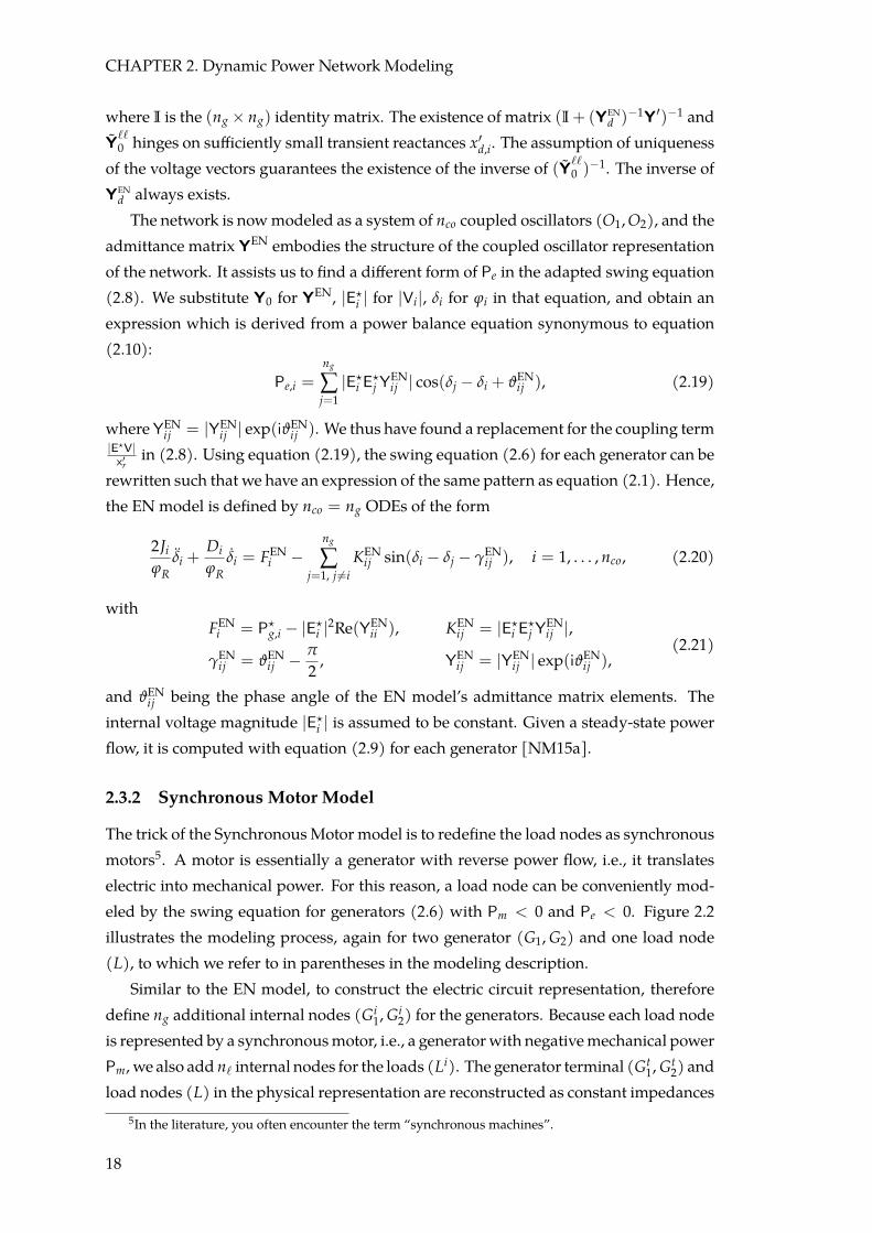
YENd always exists.The network is nowmodeled as a system of nco coupled oscillators (O1, O2), and the
admittance matrix YEN embodies the structure of the coupled oscillator representationof the network. It assists us to find a different form of Pe in the adapted swing equation(2.8). We substitute Y0 for YEN, |E?
i | for |Vi|, δi for ϕi in that equation, and obtain anexpression which is derived from a power balance equation synonymous to equation(2.10):
Pe,i =ng
∑j=1
|E?i E
?j Y
ENij | cos(δj − δi + ϑEN
ij ), (2.19)
whereYENij = |YEN
ij | exp(iϑENij ). We thus have found a replacement for the coupling term
|E?V|x′r
in (2.8). Using equation (2.19), the swing equation (2.6) for each generator can berewritten such that we have an expression of the same pattern as equation (2.1). Hence,the EN model is defined by nco = ng ODEs of the form
2Ji
ϕRδi +
Di
ϕRδi = FEN
i −ng
∑j=1, j 6=i
KENij sin(δi − δj − γEN
ij ), i = 1, . . . , nco, (2.20)
withFEN
i = P?g,i − |E?
i |2Re(YENii ), KEN
ij = |E?i E
?j Y
ENij |,
γENij = ϑEN
ij − π
2, YEN
ij = |YENij | exp(iϑEN
ij ),(2.21)
and ϑENij being the phase angle of the EN model’s admittance matrix elements. The
internal voltage magnitude |E?i | is assumed to be constant. Given a steady-state power
flow, it is computed with equation (2.9) for each generator [NM15a].
2.3.2 Synchronous Motor Model
The trick of the SynchronousMotor model is to redefine the load nodes as synchronousmotors5. A motor is essentially a generator with reverse power flow, i.e., it translateselectric into mechanical power. For this reason, a load node can be conveniently mod-eled by the swing equation for generators (2.6) with Pm < 0 and Pe < 0. Figure 2.2illustrates the modeling process, again for two generator (G1, G2) and one load node(L), to which we refer to in parentheses in the modeling description.
Similar to the EN model, to construct the electric circuit representation, thereforedefine ng additional internal nodes (Gi
1, Gi2) for the generators. Because each load node
is represented by a synchronousmotor, i.e., a generatorwith negativemechanical powerPm, we also add n` internal nodes for the loads (Li). The generator terminal (Gt
1, Gt2) and
load nodes (L) in the physical representation are reconstructed as constant impedances5In the literature, you often encounter the term “synchronous machines”.
18

2.3. The Basic Power Network Model for Load Nodes
LG1 G2
Network representation
P?`,1 P?
`,2
P?`,3
Electric Circuit representation
ix′r,3Li L
VS i2g
E3 = const.,
I 6= 0 Y`,3 = const.,
I = 0
Gt1ix′r,1Gi
1
VS i2g
E1 = const.,
I 6= 0 Yg,1 = const.,
I = 0
Gt2 ix′r,2 Gi
2
VSi2g
E2 = const.,
I 6= 0Yg,2 = const.,
I = 0
Coupled Oscillator representation
O3
F3
O1
F1
O2
F2
K13, γ13 K23, γ23
K12, γ12
G: generator node P: powerL: load node ix′r: transient reactanceO: oscillator node E: internal voltageVS: voltage source Y: equivalent admittancei2g: impedance to the ground I: current injection
Figure 2.2: Power Network Modeling Process of the SMModel
to the ground (i2g) with zero current injection. They are oncemore equatedwith trans-mission lines connecting the new generator and load internal nodes. In consequence,the mathematical formulation of the SM model is identical to the EN model and thederivation of the SM model’s admittance matrix is analogous. The SM model’s electriccircuit representation of the network has a total number of nec = 2ng + 2n` = 2n nodes.
Again, we change the node order such that indices i = 1, . . . , ng indicate the gener-ator internal nodes, i = ng + 1, . . . , n the load internal nodes, i = n + 1, . . . , n + ng gen-erator terminal nodes, and i = n + ng + 1, . . . , 2n load nodes. The diagonal admittancematrix YSM
d is now an (n × n) matrix with the generator and load transient reactances(ix′d,1)
−1, . . . , (ix′d,n)−1 on its diagonal. Parallel to the EN model, YSM
d is responsible forlinking the added generator internal and load internal nodes to the generator terminal
19

CHAPTER 2. Dynamic Power Network Modeling
and load nodes in the underlying physical network.The admittancematrixYEC′′
= YEC′′ij of size (2n× 2n) encodes the network structure
in the SM model’s electric circuit representation. Just like YEC′ above, it includes thetransient reactances of the internal and the equivalent impedances of the terminal andload nodes:
YEC′′=
[YSM
d −YSMd
−YSMd Y0 +YSM
d
]. (2.22)
Once more, we perform Kron reduction to delete all generator terminal and loadnodes (Gt
1, Gt2 and L) since these have zero current injection. To this end, let Vgi+`i be
the voltage vector corresponding to the internal nodes and Vg+` be the voltage vectorcorresponding to the generator terminal and load nodes. Kirchhoff’s current law (2.3)is then written as [
YSMd −YSM
d
−YSMd Y0 +YSM
d
] [Vgi+`i
Vg+`
]=
[Igi+`i
0
]. (2.23)
Kron reduction cuts the system size to (n × n). We get the Synchronous Motor admit-tance matrix YSM = (YSM
ij ) by using the Kron reduction formula (2.15):
YSM = YSMd (I −YSM
d (Y0 +YSMd )−1), (2.24)
where I is the (n × n) identity matrix. The structure of the coupled oscillator represen-tation is now inscribed in the entries of YSM, and all nodes are expressed as coupledoscillators (O1, O2, O3). By again replacing Y0 for YSM, |E?
i | for |Vi|, δi for ϕi in theadapted swing equation (2.9), we obtain a new statement for the active power identicalto (2.19). With nco = n, the SM model is given by the ODE system
2Ji
ϕRδi +
Di
ϕRδi = FSM
i −n
∑j=1, j 6=i
KSMij sin(δi − δj − γSM
ij ), i = 1, . . . , n, (2.25)
with
FSMi = P?
g,i − |E?i |2Re(YSM
ii ), i = 1, . . . , ng for generators,
FSMi = −P?
g,i − |E?i |2Re(YSM
ii ), i = ng + 1, . . . , n for loads/motors,
KSMij = |E?
i E?j YSM
ij |, γSMij = ϑSM
ij − π
2, YSM
ij = |YSMij | exp(iϑSM
ij ),
(2.26)
and ϑSMij being the phase angle of the SM model’s admittance matrix elements. The
constant internal voltage magnitude |E?i | is likewise computed with equation (2.9) for
each generator [NM15a].
2.3.3 Model-Dependent Parameters: Characterization and Comparison
From the derivation above, we see that the CO model equations are ODE systems ofswings equations with modeled parameters for the RHSs. The objective of this sectionis to characterize the model-dependent parameters F, K and γ.
20
2.3. The Basic Power Network Model for Load Nodes
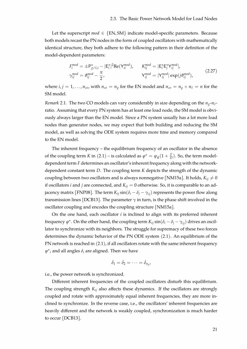
Let the superscript mod ∈ {EN, SM} indicate model-specific parameters. Becausebothmodels recast the PN nodes in the form of coupled oscillators withmathematicallyidentical structure, they both adhere to the following pattern in their definition of themodel-dependent parameters:
Fmodi = ±P?
g/`,i − |E?i |2Re(Ymod
ii ), Kmodij = |E?
i E?j Y
modij |,
γmodij = ϑmod
ij − π
2, Ymod
ij = |Ymodij | exp(jϑmod
ij ),(2.27)
where i, j = 1, . . . , nco, with nco = ng for the EN model and nco = ng + n` = n for theSM model.
Remark 2.1. The two CO models can vary considerably in size depending on the ng-n`-ratio. Assuming that every PN system has at least one load node, the SMmodel is obvi-ously always larger than the EN model. Since a PN system usually has a lot more loadnodes than generator nodes, we may expect that both building and reducing the SMmodel, as well as solving the ODE system requires more time and memory comparedto the EN model.
The inherent frequency – the equilibrium frequency of an oscillator in the absenceof the coupling term K in (2.1) – is calculated as ϕ? = ϕR(1 +
FD ). So, the term model-
dependent term F determines an oscillator’s inherent frequency alongwith the network-dependent constant term D. The coupling term K depicts the strength of the dynamiccoupling between two oscillators and is always nonnegative [NM15a]. It holds, Kij 6= 0
if oscillators i and j are connected, and Kij = 0 otherwise. So, it is comparable to an ad-jacency matrix [FNP08]. The term Kij sin(δi − δj − γij) represents the power flow alongtransmission lines [DCB13]. The parameter γ in turn, is the phase shift involved in theoscillator coupling and encodes the coupling structure [NM15a].
On the one hand, each oscillator i is inclined to align with its preferred inherentfrequency ϕ?. On the other hand, the coupling term Kij sin(δi − δj − γij) drives an oscil-lator to synchronize with its neighbors. The struggle for supremacy of these two forcesdetermines the dynamic behavior of the PN ODE system (2.1). An equilibrium of thePN network is reached in (2.1), if all oscillators rotate with the same inherent frequencyϕ?
i and all angles δi are aligned. Then we have
δ1 = δ2 = · · · = δng ,
i.e., the power network is synchronized.Different inherent frequencies of the coupled oscillators disturb this equilibrium.
The coupling strength Kij also affects these dynamics. If the oscillators are stronglycoupled and rotate with approximately equal inherent frequencies, they are more in-clined to synchronize. In the reverse case, i.e., the oscillators’ inherent frequencies areheavily different and the network is weakly coupled, synchronization is much harderto occur [DCB13].
21

CHAPTER 2. Dynamic Power Network Modeling
Based on their research, [NM15a] have implemented an open-sourceMATLAB tool-box called pg_sync_models [NM15b] which computes the model-dependent parametersF, K and γ in the ODE system of swing equations (2.1). It uses another package, MAT-POWER [ZM16], to solve the power flow equations and includes a routine to estimatethe parameters J, D and x′r which are not always provided in a power system dataset.By using these toolboxes, we have all the necessary quantities to solve system (2.1).
While the two COmodels share the same computational roots, i.e., the swing equa-tion, the classical model, and the power flow equations, it is still interesting to look atboth models. In their paper, [NM15a] demonstrate that despite their application to thesame network case, their respective CO model representations can feature utterly dif-ferent parameters F, K, γ. Likewise, applying one model on different datasets exposesdissimilar characteristics of the model parameters. In conclusion, the valid applicationof these models depends heavily on the intended goal, further assumptions, and powersystem selection [NM15a].
22

CHAPTER 3
Model Order Reduction Methods for DynamicSystems
We begin by introducing the overall problem-setup and idea of Model Order Reduc-tion, before turning our attention to the specifics of the Balanced Truncation and ProperOrthogonal Decomposition. First, we unfold the theory for linear systems, which hasbeen well studied andMORmethods have been fully fleshed out for this case (see, e.g.,[Ant05]). Because of the difficulties arising from nonlinear systems, the MOR theory isnot as evolved for this type of systems, although important nonlinear-specific conceptshave been developed, especially since the ’90s (see, e.g., [GM96; Sch93]). So, whileprimarily looking at the linear case, we point out the relevant differences particular tononlinear systems.
Throughout this thesis, we only consider continuous (i.e., time t is a real number),time-invariant systems of finite dimension.
3.1 Model Order Reduction
Problem Setup
Consider a dynamic system of (explicit) 1st-order differential equations with the statespace X ⊆ Rn, the input space U ⊆ Rm and the output/observation space Y ⊆ Rp. Itis described by state equations of the form
x(t) = f (x(t)) + g(x(t), u(t)),
y(t) = h(x(t), u(t)), (3.1)
x(0) = x0,
with variables
x(t) ∈ X state vector,
u(t) ∈ U input or excitation vector,
y(t) ∈ Y output or observation vector.
The (linear or nonlinear) functions f : Rn → Rn and g : Rn × Rm → Rn model the dy-namic behavior of the system, whereas h : Rn × Rm → Rp specifies the transformation
23

CHAPTER 3. Model Order Reduction Methods for Dynamic Systems
from the state and input to the output [Ant05; BG17]. In case, (3.1) is a linear system,it can be represented using matrices in the following way:
Definition 3.1 (State Space Description of (Linear) Dynamic System, [Ant05]). Thestate space description of a linear system is composed ofmatrices1 A ∈ Rn×n, B ∈ Rn×m
and C ∈ Rp×n, such that
x(t) = Ax(t) + Bu(t),
y(t) = Cx(t), (3.2)
x(0) = x0,
with x(t) ∈ Rn, u(t) ∈ Rm, and y(t) ∈ Rp, and a given initial value x0. We conciselydenote this system by
Σ =
(A B
C
)∈ R(n+p)×(n+m). (3.3)
Corresponding to the respective functions, A and B are the state dynamics and inputmatrices, respectively, and C is the output matrix.
Definition 3.2 (Complexity, Order, [Ant05; AS01]). The complexity, or order of a system(3.1) is defined as the number n of state variables included, i.e., the size of the statevector x = (x1, · · · , xn)∗, or the number of state equations, respectively.
Using the matrix exponential defined by
eMt = In +t1!
M +t2
2!M2 + · · ·+ tk
k!Mk + · · · , (3.4)
for a matrix M ∈ Rn×n and a scalar t ∈ R, the solution of the state equations in system(3.2) at time t > t0 is
ψ(u; x0; t) = eA(t−t0)x0 +∫ t
t0
eAt−τBu(τ)dτ, (3.5)
provided an input u, and an initial condition x(0) = x0 at time t0. The output is accord-ingly,
y(t) = Cψ(u; x(t0); t) = Cψ(0; x(t0); t) + Cψ(u; 0; t) (3.6)
accordingly, [Ant05].
Idea of Model Order Reduction
In the introduction in Chapter 1, we mentioned some of the challenges posed by large-scale system, e.g., constraints on computation time, storage and accuracy. To circumvent
1The output equations can have an additional term D : Rm → Rp mapping u, but since this map isirrelevant in this thesis, we omit it.
24

3.1. Model Order Reduction
these impairments, a simplified model is needed which can be used instead of the orig-inal system for simulation or control purposes.
The objective of Model Order Reduction is to find a dynamic system of lower or-der nρ � n that can be used instead of the FOM. This reduced-order model can berepresented in form of a system of equations relating to system (3.1),
˙x(t) = f (x(t)) + g(x(t), u(t)),
y(t) = h(x(t), u(t)), (3.7)
x(0) = x0,
with
f : Rnρ → Rnρ , g : Rnρ × Rm → Rnρ , h : Rnρ × Rm → Rp,
or, corresponding to (3.2), a system of matrices,
˙x(t) = Ax(t) + Bu(t),
y(t) = Cx(t), (3.8)
x(0) = x0,
with matrices A ∈ Rnρ×nρ , B ∈ Rnρ×m and C ∈ Rp×nρ .
Definition 3.3 ((Linear) reduced-order model, [Ant05]). We denote the reduced-ordermodel of the full-order model Σ in (3.3) by
Σ =
(A B
C
)∈ R(nρ+p)×(nρ+m), (3.9)
with reduction order nρ � n.
Figure 3.1 illustrates the MOR process for linear systems.
A
C
B A
C
B
Figure 3.1: Graphical Depiction of MOR Process for Linear Systems
The ROM should approximate the original FOM (3.3) such that it meets certain re-quirements, for example:2: (1) The foremost is, of course, that the ROM is of lowercomplexity, i.e., nρ � n. (2) The error between the full- and the reduced-order systemis small. The existence of a global error bound is also desirable. (3) System properties
2A more elaborate list can be found in [Ant05; AS01].
25

CHAPTER 3. Model Order Reduction Methods for Dynamic Systems
like stability are maintained. (4) The computation itself is stable and efficient [Ant05;AS01; BG17].
The first two requirements considered together imply that the MORmethod shouldprovide some decision-making tool or measure to determine which states to discardand which ones to preserve, i.e., which states are either too “important” to cut and/orwhich states are “not important enough” to keep in order to achieve a small reductionerror.
Essential Methods
Themost fundamental technique needed inMOR is the state transformation. The inten-tion is to bring the system into a new form such that the MOR method can take advan-tage of certain structural properties. We require a nonsingular matrix T transformingthe state variable
x = Tx, (3.10)
and applied to the system matrices accordingly, system (3.2) is transformed into
˙x = TAT−1︸ ︷︷ ︸A
x + TB︸︷︷︸B
u,
y = CT−1︸ ︷︷ ︸C
x.
So, by means of T, we can transform system Σ in (3.3) into an equivalent system Σ,(3.9), i.e., (
TIp
)(A B
C
)︸ ︷︷ ︸
Σ
=
(A B
C
)︸ ︷︷ ︸
Σ
(T
Im.
)(3.11)
In this thesis, we test the Balanced Truncation (BT) method to reduce the COmodelsystems. It is a Singular Value Decomposition (SVD)-basedMOR approach. Because ofthe SVD’s importance, we briefly revisit it here alongwith the Cholesky decomposition,another significant decomposition used in BT.
Theorem 3.4 (Singular Value Decomposition, [Ant05]). Let M ∈ Cn×k with n 6 k andσi =
√λi > 0, where λi the i-th eigenvalue (EV) of M∗M. Then, there exists a decomposition
M = VΣW∗, (3.12)
where V = (v1 · · · vn) ∈ Cn×n and W = (w1 · · ·wk) ∈ Ck×k are unitary matrices andΣ = diag(σ1, . . . , σn) is a diagonal matrix with the singular values (SVs) σi arranged in de-creasing order σ1 > σ2 > · · · > σn > 0. The vi’s and wj’s are the left and right singular vectorsof M, respectively.
26

3.2. Balanced Truncation for (Linear) Dynamic Models
Theorem3.5 (CholeskyDecomposition, [Hig96]). Let M ∈ Rn×n be a symmetric positivedefinite matrix. Then, there exists a unique decomposition
M = R∗R, (3.13)
where the Cholesky factor R ∈ Rn×n is an upper triangular matrix with positive elements onits diagonal.
3.2 Balanced Truncation for (Linear) Dynamic Models
In this section, we introduce the concepts of reachability and observability. They give us ameasure to determinewhich states are important in a system. Balanced Truncation usesthese concepts as the aforementioned “cut-or-keep” decision-making tool. A number ofstates in a dynamic systemmight be difficult to reachwhile the states which are difficultto observemight be different ones. This difficulty ismeasured by the degree of reachabilityand degree of observability, respectively. BT balances the system first such that the statesto truncate are simultaneously hard to reach and observe.
Let X ⊆ Rn be the state space throughout this section.
The Reachability Concept
In this subsection, we only consider systems of the form Σ =
(A B
), since the output
matrix C is of no consequence regarding reachability. The concept estimates howmuchthe system’s state x can be influenced by the input u.
Definition 3.6 (Reachability Terminology, [Ant05]).
• A point x ∈ X is reachable from the zero state, if there is an input function u(t) offinite energy and a time T < ∞, such that
x = ψ(u; 0; T)
is fulfilled.
• All the reachable states in Σ make up the reachable subspace Xreach ⊆ X. The systemΣ is (completely) reachable if Xreach = X.
• The reachability matrix of Σ is defined as
R(A, B) =[
B AB A2B · · · An−1B · · ·]
. (3.14)
Due to the Cayley-Hamilton theorem, the first n terms of the reachability matrix aresufficient to determine its rank and span. This allows us to use the finite reachabilitymatrix Rn(A, B) =
[B AB A2B · · · An−1B
]in computational settings3.
3For properties of the reachability matrix and its connection to the reachability Gramian, see Ap-pendix A.1.
27

CHAPTER 3. Model Order Reduction Methods for Dynamic Systems
We now introduce the first stepping-stone towards measuring the reachability of astate.
Definition 3.7 (Finite Reachability Gramian, [Ant05]). For a time t < ∞, the finitereachability Gramian is given by
P(t) =∫ t
0eAτBB∗eA∗τdτ. (3.15)
From the definition follows that the finite reachability Gramian is positive semidef-inite, i.e., P(t) = P∗(t) > 0.
Theorem3.8 (ReachabilityConditions, [Ant05]). The following statements are equivalent:
1. The system Σ containing (A, B) is reachable.
2. The reachability matrix R(A, B) has full rank.
3. The reachability Gramian P(t) is positive definite for some t > 0.
The concept of controllability is equivalent to the reachability concept, which in awayreverses the latter: Controllability considers how an input u can direct the system froma given nonzero state to the zero state rather thanmoving the system from the zero stateto a specific state.
Definition 3.9 (Controllable state; controllable subspace, [Ant05]).
• A(nonzero) point x ∈ X is controllable to the zero state, if there is an input functionu(t) with finite energy and a time T < ∞, such that
ψ(u; x; T) = 0
is fulfilled.
• All the reachable states in Σ make up the controllable subspace Xcontr ⊆ X. IfXcontr = X, the system Σ is (completely) controllable.
The equivalence of the reachability and controllability concepts is established by
Theorem 3.10 (Reachability-Controllability Equivalence, [Ant05]). Xreach = Xcontr.
The Observability Concept
In order to steer and evaluate the dynamics of a system, knowledge of the state vari-ables is necessary. As these data frequently cannot be measured, the state observationproblem is concerned with the inference of the state variables x(T) from outputs (orobservations) y(τ), where τ ∈ [T, T + t].
Without loss of generality, the observation problem can be simplified by assumingthat T = 0. We can also assume, that u(·) = 0. As we know the input u, for t > 0 the last
28

3.2. Balanced Truncation for (Linear) Dynamic Models
term in (3.6) is known, too. Thus, the task at hand is to find x(0), given Cψ(0, x(0), t)
for t > 0. These assumptions hold throughout this subsection and render input matrix
B redundant. Hence, we consider the system Σ =
(A
C
).
Definition 3.11 (Observability Terminology, [Ant05]).
• A point x ∈ X is unobservable if y(t) = Cψ(0, x, t) = 0 for all t > 0.
• All the unobservable states in Σ make up the unobservable subspace Xunobs ⊆ X.
• If Xunobs = 0, the system Σ is (completely) observable.
• The observability matrix of Σ is defined as
O(C, A) =[C∗ A∗C∗ (A∗)2C∗ · · · (A∗)n−1C∗ · · ·
]∗. (3.16)
Once more, the Cayley-Hamilton theorem permits us to work with the finite ob-servability matrix On(C, A, ) =
[C∗ A∗C∗ (A∗)2C∗ · · · (A∗)n−1C∗]∗ in computational
contexts4.We presently define the second stepping-stone towards computing the observability
of a system.
Definition 3.12 (Finite Observability Gramian, [Ant05]). For a time t < ∞, the finiteobservability Gramian is given by
Q(t) =∫ t
0eA∗τC∗CeAτdτ. (3.17)
Theorem 3.13 (Observability Conditions, [Ant05]). The following statements are equiv-alent:
1. The system Σ containing (C, A) is observable.
2. The observability matrix O(C, A) has full rank.
3. The observability Gramian Q(t) is positive definite for some t > 0.
Infinite Gramians and Energy Functionals
In this subsection, we derive an important feature of the Gramians which provides thewanted state importance measure. We first introduce one more necessary assumption.To this purpose, we assume u ≡ 0 and consider the autonomous system
x(t) = Ax(t). (3.18)4For properties of the observabilitymatrix and its link to the observability Gramian, see Appendix A.1.
29

CHAPTER 3. Model Order Reduction Methods for Dynamic Systems
Definition 3.14 (Stable Matrix, [Ant05; Zha13]). A matrix is stable if its eigenvalues λ
are in the left half of the complex plane, or put differently, Re(λ) < 0 for all eigenvaluesλ.
A matrix is called semi-stable if the real part of every eigenvalue λ is nonpositive, i.e.,Re(λ) 6 0 for all eigenvalues λ.
Theorem 3.15 relates a stable linear dynamics matrix A to an (asymptotically) stablesystem Σ.
Theorem 3.15 (Matrix-based System Stability, [Ant05]). The system x(t) = Ax(t) is
(1) stable if and only if for all eigenvalues λ of A it holds Re(λ) 6 0 and the multiplicity ofthose eigenvalues with Re(λ) = 0 is one.
(2) asymptotically stable if and only if the matrix A is stable.
Remark 3.16. We equate stability with asymptotic stability from now on [Ant05]. For amore in-depth treatment of stability, we refer to Appendix A.2.
We now consider a stable system Σ =
(A B
C
). LetLn
p(I) be the space of Lebesgue-
integrable functions equipped with a p-norm over some finite or infinite interval I , i.e.,
Lnp(I) = { f : I → Rn, || f ||p < ∞}, 1 6 p 6 ∞. (3.19)
The 2-norm of a function f defines its energy
|| f ||2 = 〈 f , f 〉 =∫ T
0f ∗(t) f (t)dt.
Our objective is to compute the energy functionals of the system.
Definition 3.17 (Controllability andObservability Energy Functionals, [Sch93]). Thecontrollability energy functional of a system is defined as
Lc(x0) = minu∈L2(−∞,0)x(−∞)=0, x(0)=0
=12
∫ 0
−∞||u(t)||2dt. (3.20)
It is the minimum amount of energy needed to steer the system from the zero state attime t = −∞ to x(0) = x0.
Likewise, the observability energy functional of a system is defined as
Lo(x0) =12
∫ ∞
0||y(t)||2dt, (3.21)
where x(0) = x0 and u(t) = 0 for 0 6 t < ∞. It is the amount of energy generated bythe initial state x0 with no input present.
30
3.2. Balanced Truncation for (Linear) Dynamic Models
Comparing these functionals with Theorems 3.9 and 3.11, it is apparent, they giveus a measure of the degree of controllability (or equivalently the degree of reachability) anddegree of observability, respectively [Ant05]. Intuitively, we would like to minimize theenergy it takes to control the system andmaximize the produced energywe can observefrom the system.
We can compute time-dependent values for the energy functionalswith finiteGrami-ans, see Proposition A.12 in Appendix A.3. However, it is desirable to have a time-independent measure. Since we assume a stable system with a stable matrix A, theintegrals of both types of finite Gramians are bound as we let t → ∞. Thus, we candefine infinite versions of the reachability Gramian 3.7 and observability Gramian 3.12.That is for t = ∞, we have the following definition.
Definition 3.18 (Infinite Gramians, [Ant05]).
P =∫ ∞
0eAτBB∗eA∗τdτ, (3.22)
Q =∫ ∞
0eA∗τC∗CeAτdτ. (3.23)
To compute them, we solve the so-called Lyapunov equations.
Theorem 3.19 (Lyapunov Equations, [Ant05]). The infinite Gramians are the unique so-lutions to the Lyapunov equations
AP + PA∗ + BB∗ = 0, (3.24)
A∗Q+QA + C∗C = 0. (3.25)
Remark 3.20. In Appendix A.2, we present a nice connection between Lyapunov equa-tions and another type of stability based on a special kind of scalar functions, the so-called Lyapunov functions.
If we additionally assume (complete) reachability and observability of the system,the Gramians are positive definite and by the properties of the integral, we have
P > P(t), and Q > Q(t), for all t.
Keeping this observation in mind, we can compute optimized values of the energyfunctionals with the infinite Gramians as the following Theorem 3.21 states.
Theorem 3.21 (Computation of Energy Functionals, [Ant05; Sch93]). Let the infiniteGramians P and Q be the unique solutions to the Lyapunov equations in Theorem 3.19. Then,
Lc(x0) =12
x∗0P−1x0, (3.26)
which is the minimal control energy needed to arrive at the state x0, and
Lo(x0) =12
x∗0Qx0, (3.27)
which is the maximal observation energy generated by the initial state x0.
31

CHAPTER 3. Model Order Reduction Methods for Dynamic Systems
Nowweknowhow to optimize the energy functionals. Ifwe therefore look at the im-portance of state variables from an energetic point of view, this theorem helps us to dis-tinguish the significant from the insignificant states. In terms of energy, the stateswhichrequire the most energy to control lie in the span of eigenvectors of P relating to smalleigenvalues. Likewise, the states which cause the least observation energy lie in theeigenvector span of Q relating to small eigenvalues. The size of these sub-eigenspacesprovide the degree of controllability/reachability and degree of observability [Ant05].
Balancing and Truncating
These degrees guide the decision which states to cut and which to keep. However, asthesemeasures are basis-dependent, it might occur that states which are hard to controlare not hard to observe or the other way around. Balanced Truncation makes sure toonly omit those states for which the difficulty to control and observe coincide.
Mathematically, this amounts to express P and Q in a common basis. It requires asuitable similarity transformation which warrants that
P = TPT∗, Q = T−∗QT−1 ⇒ PQ = T(PQ)T−1. (3.28)
The transformationmatrix T is then called a balancing transformation and its columnsare the eigenvectors of the product PQ. It follows that the product of the Gramians ofequivalent systems have the same eigenvalues. This in turn guarantees that the stateswhich are difficult to control are identical to the states which are difficult to observe.
Definition 3.22 (Balanced System, [Ant05]). The stable, reachable and observable sys-tem Σ is balanced if P = Q. If in addition
P = Q = Σ = diag (σ1, . . . , σn) ,
the system is principal-axis balanced.
The values on the diagonal are special system invariants, called the Hankel singularvalues [Ant05]:
Lemma 3.23 (Hankel Singular Values, [Ant05]). TheHankel singular values of the bal-anced system Σ are equal to the positive square roots of the eigenvalues (EVs) of the product ofthe infinite Gramians, that is
σi(Σ) =√
λi(PQ), i = 1, . . . , n, (3.29)
with σi > σi+1.
Evidently, in a balanced system large eigenvalues of the product PQ correspondto large Hankel singular values. The decay rate of these SVs indicates an appropriatereduction order nρ.
32

3.3. Balanced Truncation for (Quadratic) Dynamic Models
There are several ways to determine a balancing transformation. One approach usesthe eigenvalue decomposition. But since this requires the computation of two matrixinverses, we present the square root method here.
First, we decompose both P and Q into their respective Cholesky factors,
P = R∗R and Q = S∗S . (3.30)
The SVs of the product of the Cholesky factors R and S∗ are precisely the HankelSVs. So, we compute the SVD
RS∗ = VΣW∗, (3.31)
and get the orthogonal matrices V and W. The balancing matrix is then
T = Σ−1/2W∗S with T−1 = R∗VΣ−1/2. (3.32)
We apply T to system (3.3) as in (3.11) and receive the balanced, equivalent system(TAT−1 TB
CT−1
). (3.33)
Now for the reduction, we partition V =(
Vnρ Vn−nρ
)and W =
(Wnρ Wn−nρ
),
Vnρ , Wnρ ∈ Rn×nρ , where nρ is the number of the nρ largest SVs of Σ, such that
RS∗ = VΣW∗ ≈ Vnρ ΣnρW∗nρ
. (3.34)
The nρ leading columns of V span a low-dimensional space in which the state vectorx(t) can be approximated by another vector x(t). We set the transformation matrices
W∗ = Tnρ = Σ− 12
nρW∗
nρS , V = T−1
nρ= R∗Vnρ Σ− 1
2nρ
, (3.35)
where Σnρ is the upper left nρ × nρ-block of Σ. The state vector can then be approxi-mated by x ≈ V x with x(t) ∈ Rnρ , which relates the ROM to the FOM, and we obtainthe ROM
Σ =
(W∗AV W∗B
CV
)(3.36)
of reduction order nρ � n.
3.3 Balanced Truncation for (Quadratic) Dynamic Models
A lot of concepts and ideas of MOR and BT remain valid under nonlinear conditions,still there are some important peculiarities. Because we lack a holistic nonlinear MORtheory, we focus on those which arise in the context of quadratic systems.
33

CHAPTER 3. Model Order Reduction Methods for Dynamic Systems
Structural Adaptations to Problem Setup and Balancing Measurement
The problem setup for nonlinear MOR is almost the same, except that at least one of thefunctions in system (3.1) and one of themaps in system (3.3) is explicitly nonlinear. Thesystemmight also have additional functions and corresponding matrix representationswhich model the nonlinear behavior of the system.
In the following considerations, we assume that the state of the system is the zerostate at time t = 0, i.e., the initial condition is x(0) = x0 = 0. If x(0) = x0 6= 0 wecan define suitable state variables x = x − x0 and transform the system accordingly, seesection 4.3 for the treatment of our specific case, or [BBF14] for linear time-invariantsystems.
We base our MOR efforts on nonlinear systems with a quadratic5 structure6 Theirstate space description is analogous to Definition 3.1:
Definition 3.24 (State Space Description of Quadratic Dynamic System). Given ma-trices A ∈ Rn×n, H ∈ Rn×n2
, B ∈ Rn×m and C ∈ Rp×n, the state space description of aquadratic dynamic system is
x(t) = Ax(t) + H(x(t)⊗ x(t)
)+ Bu(t),
y(t) = Cx(t),
x(0) = 0,
(3.37)
with x(t) ∈ Rn, u(t) ∈ Rm, and y(t) ∈ Rp. The compact notation is
Σ =
(A H B
C
)∈ R(n+p)×(n+n2+m). (3.38)
Matrices A and H model the linear and quadratic state dynamics, respectively, B is theinput matrix, and C is the output matrix.
Remark 3.25. The symbol ⊗ depicts the Kronecker product. For the definition and prop-erties, we refer to Appendix B.1
The objective of the quadratic MOR is to find a reduced dynamic system complexitynρ � n (compare to (3.8)),
˙x(t) = Ax(t) + H(x(t)⊗ x(t)
)+ Bu(t),
y(t) = Cx(t),
x(0) = 0,
(3.39)
with
A ∈ Rnρ×nρ , H ∈ Rnρ×n2ρ , B ∈ Rnρ×m, C ∈ Rp×nρ ,
5This involves the use of the Kronecker product. For its definition and properties, see Appendix B.1.6Our BT approach is based on the paper [BG17]. The authors actually deal with quadratic-bilinear
systems, but since the bilinear term is irrelevant in our case, we omit it.
34

3.3. Balanced Truncation for (Quadratic) Dynamic Models
which approximates the quadratic system (3.37) such that it satisfies the aforemen-tioned requirements on Page 26. Figure 3.2 illustrates the MOR process for quadraticsystems.
A H
C
B A H
C
B
Figure 3.2: Graphical Depiction of MOR Process for Quadratic Systems
Definition 3.26 (Quadratic Reduced-Order Model). We denote the quadratic reduced-order model of system (3.38) by
Σ =
(A H B
C
)∈ R(nρ+p)×(nρ+n2
ρ+m) (3.40)
with reduction order nρ � n (compare to Definition 3.3).
The basic idea and procedure of Balanced Truncation are identical to the linear case.But just like the problem setup, the key BT-specific concepts need to be modified to thequadratic case. We begin this adaptation process with the energy functionals whichprovide the measures of where and how much to truncate the system.
The definition of the controllability energy functional in Definition 3.17 holds for thenonlinear case. However, the definition given for the observability energy functionalassumes that the system is zero-state observable, i.e., if both input and output variablesare zero for t > 0, the state variable must remain at zero for all t > 0. This assumptionis too strong for nonlinear systems. In [BG17], the authors overcome this restriction byrequiring the input to be L2- and L∞-bounded.
Definition 3.27 (Relaxed Observability Energy Functional, [BG17]). The observabil-ity energy functional of a nonlinear system is defined as
Lo(x0) = maxu∈K(κ,β)
x(0)=x0, x(∞)=0
=12
∫ ∞
0||y(t)||2dt, (3.41)
where K(κ,β) = {u ∈ Lm2 [0, ∞) : ||u||L2 6 κ, ||u||L∞ 6 β}.
This definition evaluates the state variables from a state-to-output perspective. Astate component would be deemed irrelevant if it has the least share in the observabilityenergy for every conceivable input within the L2- and L∞-bounded ball [BG17; GM96].
In the linear context, the controllability and observability energy functionals can bestated in terms of a plain quadratic formula, as seen in Theorem 3.21. For nonlinear
35

CHAPTER 3. Model Order Reduction Methods for Dynamic Systems
systems, this is not possible, not even with the limitation to quadratic systems. Nev-ertheless, [BG17] contribute bounds on the energy functionals. The goal of the nextsubsections of this thesis is to derive and compute the truncated quadratic Gramianswhich provide the following bounds:
Theorem 3.28 (Energy Functional Bounds with Truncated Gramians, [BG17]7). Con-sider system (3.37) with a stable matrix A. Assume the system to be locally reachable andobservable. Let the truncated reachability Gramian PT > 0 and the observability GramianQT > 0 satisfy their respective Lyapunov equation (3.48) and (3.54). Then,
(1) there is a neighborhood Kc of 0, such that for x ∈ Kc
Lc(x) >12
x∗P−1T x. (3.42)
(2) Likewise, there is a neighborhood Ko of 0, such that for x ∈ Ko
Lo(x) 612
x∗QT x. (3.43)
In their paper, [BG17] give an example which shows that close to the origin theenergy functionals based on the truncated Gramians do not only present a good ap-proximate to the actual energy functionals computed by solving the partial differentialequations (see TheoremA.14 ), but indeed outperform the energy functionals based onthe infinite Gramians.
Reachability Gramians
To find an expression for the reachability Gramian, [BG17] make use of the Volterra se-ries, a well-established method for bilinear systems (see, e.g., [BGR17; BPK71; Rug81]).They treat the quadratic-bilinear case similarly to this type of nonlinear systems.
The Volterra series restates a nonlinear system in terms of cascaded linear (sub-)systems by a functional series expansion8 [BPK71; VG18]. There are various ways toconstruct a Volterra Series representation of a system (see, e.g., [Rug81; VG18]). Wemerely illustrate the first few steps in the derivation of the series for quadratic systemsto give an idea of the procedure and stick to the straightforward approach taken by[BG17] for simplicity.
We start by defining the notation
xτ1,...,τ`(t) := x(t − τ1 − · · · − τ`), uτ1,...,τ`(t) := u(t − τ1 − · · · − τ`),
7See Theorem A.15 for the version with infinite Gramians.8In particular, a Volterra series expansion is often used to formulate an input-output representation of a
nonlinear system in order to linearize the systemor to derive transfer functions [BPK71; Fla12; Isi85; Rug81;VG18]. As a we do not seek a different output representation, we focus exclusively on the restatement ofthe state equation, just like [BG17].
36
3.3. Balanced Truncation for (Quadratic) Dynamic Models
and integrate both sides of the state equation of system (3.37) in the state variables withrespect to time. Thus, we get
x(t) =∫ t
0eAτ1 Buτ1(t)dτ1 +
∫ t
0eAτ1 H
(xτ1(t)⊗ xτ1(t)
)dτ1. (3.44)
As we need the value of xτ1(t), we proceed analogously to (3.44), and obtain the sameintegral solution, but with adapted integration limits and differential, i.e.,
xτ1(t) =∫ t−τ1
0eAτ2 Buτ1,τ2(t)dτ2 +
∫ t−τ1
0eAτ2 H
(xτ1,τ2(t)⊗ xτ1,τ2(t)
)dτ2.
So, xτ1(t) computes part of the time interval of x(t). Now, we substitute xτ1(t) in (3.44),but switch the differential of the second quadratic term from τ2 to τ3. Since the inte-gration limit remains unchanged this is of no consequence for the computation of theintegral. With this trick, we create a pseudo-linear equation and acquire
x(t) =∫ t
0eAτ1 Buτ1(t)dτ1
+∫ t
0eAτ1 H
( [∫ t−τ1
0eAτ2 Buτ1,τ2(t)dτ2 +
∫ t−τ1
0eAτ2 H
(xτ1,τ2(t)⊗ xτ1,τ2(t)
)dτ2
]⊗[∫ t−τ1
0eAτ3 Buτ1,τ3(t)dτ3 +
∫ t−τ1
0eAτ3 H
(xτ1,τ3(t)⊗ xτ1,τ3(t)
)dτ3
] )dτ1
(/)=∫ t
0eAτ1 Buτ1(t)dτ1
+∫ t
0eAτ1 H
( [∫ t−τ1
0eAτ2 Buτ1,τ2(t)dτ2 ⊗
∫ t−τ1
0eAτ2 Buτ1,τ3(t)dτ3
]+
[∫ t−τ1
0eAτ2 H
(xτ1,τ2(t)⊗ xτ1,τ2(t)
)dτ2 ⊗
∫ t−τ1
0eAτ3 Buτ1,τ3(t)dτ3
]+
[∫ t−τ1
0eAτ2 Buτ1,τ2(t)dτ2 ⊗
∫ t−τ1
0eAτ3 H
(xτ1,τ3(t)⊗ xτ1,τ3(t)
)dτ3
]+
[∫ t−τ1
0eAτ2 H
(xτ1,τ2(t)⊗ xτ1,τ2(t)
)dτ2 ⊗
∫ t−τ1
0eAτ3 H
(xτ1,τ3(t)⊗ xτ1,τ3(t)
)dτ3
] )dτ1,
wherewe used the distributivity property of the Kronecker product in (/) (3rd propertyin Theorem B.2). Pulling out the integral and switching the order of integration using
37

CHAPTER 3. Model Order Reduction Methods for Dynamic Systems
Fubini’s theorem, this equals
x(t) =∫ t
0eAτ1 Buτ1(t)dτ1
+∫ t
0
∫ t−τ1
0
∫ t−τ1
0eAτ1 H
( [eAτ2 Buτ1,τ2(t)⊗ eAτ3 Buτ1,τ3(t)
]+[eAτ2 H
(xτ1,τ2(t)⊗ xτ1,τ2(t)
)⊗ eAτ3 Buτ1,τ3(t)
]+[eAτ2 Buτ1,τ2(t)⊗ eAτ3 H
(xτ1,τ3(t)⊗ xτ1,τ3(t)
)]+[eAτ2 H
(xτ1,τ2(t)⊗ xτ1,τ2(t)
)⊗ eAτ3 H
(xτ1,τ3(t)⊗ xτ1,τ3(t)
)] )dτ1dτ2dτ3
(O)=
∫ t
0eAτ1 Buτ1(t)dτ1
+∫ t
0
∫ t−τ1
0
∫ t−τ1
0eAτ1 H
( [(eAτ2 B ⊗ eAτ3 B)(uτ1,τ2(t)⊗ uτ1,τ3(t))
]+[eAτ2 Buτ1,τ2(t)⊗ eAτ3 H
(xτ1,τ3(t)⊗ xτ1,τ3(t)
)]+[eAτ2 H
(xτ1,τ2(t)⊗ xτ1,τ2(t)
)⊗ eAτ3 Buτ1,τ3(t)
]+[eAτ2 H
(xτ1,τ2(t)⊗ xτ1,τ2(t)
)⊗ eAτ3 H
(xτ1,τ3(t)⊗ xτ1,τ3(t)
)] )dτ1dτ2dτ3,
where we used the mixed product property in (O) (5th property in Theorem B.2). Con-tinuing to substitute for the state variables generates the Volterra series for the quadraticsystem. From this, the so-called Volterra kernels can be identified.
Definition 3.29 (Reachability Mapping, Volterra Kernels, [BG17]). We define thereachability mapping P = [P1, P2, P3, . . .]9 with the Pi’s being the Volterra kernels deducedfrom the Volterra series:
P1(t1) = eAt1 B,
P3(t1, t2, t3) = eAt3[H[P1(t1)⊗ P1(t2)]
]= eAt3
[H[(eAt1 B)⊗ (eAt2 B)]
]P5(t1, . . . , t5) = eAt5
[H[P1(t1)⊗ P3(t2, t3, t4), P3(t1, t2, t3)⊗ P1(t4)]
],
= eAt5[H[(eAt1 B)⊗ (eAt4 [H(eAt2 B ⊗ eAt3 B)]),
(eAt3 [H(eAt1 B ⊗ eAt2 B)])⊗ (eAt4 B)],...
Pi(t1, . . . , ti) = eAti[H[P1(t1)⊗ Pi−2(t2, . . . , ti−1),
P2(t1, t2)⊗ Pi−3(t3, . . . , ti−1),
. . . , Pi−2(t1, . . . , ti−2)⊗ P1(ti−1)]], for all i > 3, i ≡ 1 mod 2,
and Pi(t1, . . . , ti) = 0 for all i ≡ 0 mod 2.
9To avoid confusion concerning the indices used in [BG17], we adhere to the numbering given in thatpaper. So, all the even numbered kernels are 0 here, because the bilinear term is N = 0.
38

3.3. Balanced Truncation for (Quadratic) Dynamic Models
Definition 3.30 (Reachability Gramian, [BG17]). The reachability Gramian P is definedby means of P as
P =∞
∑i=1
Pi with Pi =∫ ∞
0· · ·
∫ ∞
0Pi(t1, . . . , ti)P∗
i (t1, . . . , ti)dt1 · · ·dti. (3.45)
The summands of the reachability Gramian satisfy a sequence of a special type ofquadratic Lyapunov equations. Consider the first summand in Definition 3.30,
P1 =∫ ∞
0P1P∗
1 dt1 =∫ ∞
0eAt1 BB∗eA∗t1dt1.
This is just the linear infinite Gramian of Definition 3.18. As stated in Theorem 3.19,under the assumption that A is stable, it is the solution of the Lyapunov equation
AP1 + P1A∗ + BB∗ = 0. (3.46)
For P3, we have
P3 =∫ ∞
0
∫ ∞
0
∫ ∞
0P3P∗
3 dt1dt2dt3
=∫ ∞
0
∫ ∞
0
∫ ∞
0eAt3
[H[P1(t1)⊗ P1(t2)][P1(t1)⊗ P1(t2)]
]∗H∗eA∗t3dt1dt2dt3
=∫ ∞
0
∫ ∞
0
∫ ∞
0eAt3
[H[(eAt1 B)⊗ (eAt2 B)][(eAt1 B)⊗ (eAt2 B)]∗H∗]eA∗t3dt1dt2dt3
(.)=∫ ∞
0
∫ ∞
0
∫ ∞
0eAt3
[H[(eAt1 B)⊗ (eAt2 B)][(eAt1 B)∗ ⊗ (eAt2 B)∗]H∗]eA∗t3dt1dt2dt3
(O)=∫ ∞
0
∫ ∞
0
∫ ∞
0eAt3
[H[(eAt1 B)(eAt1 B)∗]⊗ [(eAt2 B)(eAt2 B)∗]H∗]eA∗t3dt1dt2dt3
=∫ ∞
0
∫ ∞
0
∫ ∞
0eAt3
[H[(eAt1 BB∗eA∗t1)]⊗ [(eAt2 BB∗eA∗t2)]H∗]eA∗t3dt1dt2dt3
=∫ ∞
0eAt3
[H[∫ ∞
0(eAt1 BB∗eA∗t1)dt1]︸ ︷︷ ︸
P1
⊗ [∫ ∞
0(eAt2 BB∗eA∗t2)dt2]︸ ︷︷ ︸
P1
H∗]eA∗t3dt3
=∫ ∞
0eAt3
[H(P1 ⊗ P1)H∗]eA∗t3dt3,
whereweused the distributivity of (conjugate) transposition in (.) and themixedprod-uct property of the Kronecker product in (O) (the 4th and 5th property in Theorem B.2).So, the term P3 can be expressed as a function of the preceding term P1 and is the solu-tion to the Lyapunov equation [BG17],
AP3 + P3A∗ + H(P1 ⊗ P1)H∗ = 0. (3.47)
Carrying on in the same manner with the succeeding Pi’s, we see that each of these
39

CHAPTER 3. Model Order Reduction Methods for Dynamic Systems
multiple integrals can be broken down into parts consisting of its predecessors, i.e.,
Pi =∫ ∞
0· · ·
∫ ∞
0Pi P∗
i dt1 · · ·dti
=∫ ∞
0eAti
[H[( ∫ ∞
0P1(t1)P∗
1 (t1)dt1
)⊗( ∫ ∞
0· · ·
∫ ∞
0Pi−2(t2, . . . , ti−1)P∗
i−2(t2, . . . , ti−1)dt2 · · ·dti−1
)+ · · ·+
( ∫ ∞
0· · ·
∫ ∞
0Pi−2(t1, . . . , ti−2)P∗
i−2(t1, . . . , ti−2)dt1 · · ·dti−2
)⊗( ∫ ∞
0P1(ti−1)P∗
1 (ti−1)dti−1
)]H∗]
eA∗tidti
and solve the Lyapunov equation
APi + Pi A∗ + H(P1 ⊗ Pi−2 + P3 ⊗ Pi−3 + · · ·+ Pi−3 ⊗ P3 + Pi−2 ⊗ P1)H∗ = 0. (3.48)
When we sum up equations (3.46), (3.47) and (3.48), we have
A∞
∑i=1
Pi︸ ︷︷ ︸P
+∞
∑i=1
Pi︸ ︷︷ ︸P
A∗ + H( ∞
∑i=1
Pi︸ ︷︷ ︸P
⊗∞
∑i=1
Pi︸ ︷︷ ︸P
)H∗ + BB∗ = 0, (3.49)
which implies the following theorem,
Theorem 3.31 (Reachability Gramian Lyapunov Equation, [BG17]). Consider system(3.37) and let A be stable. Assuming that the reachability Gramian P as defined in 3.30 exists,it is the solution of the generalized quadratic Lyapunov equation
AP + PA∗ + H(P ⊗P)H∗ + BB∗ = 0. (3.50)
Observability Gramians
The derivation and results for the reachability Gramian are parallel to those which canbe obtained for the observability Gramian. We simply state the definitions and conclu-sions for this Gramian here.
Definition 3.32 (ObservabilityMapping, Volterra Kernels, [BG17]). Let the Pi’s be asin Definition 3.29, and let H(2) be the mode-2 unfolding of a tensor constructed fromH10. Furthermore, let the Qi’s be the Volterra kernels deduced from the Volterra series,
10For details, see Appendix B.2.
40

3.3. Balanced Truncation for (Quadratic) Dynamic Models
and let Q = [Q1, Q2, Q3, . . .]11 be the observability mapping made up of these kernels:
Q1(t1) = eA∗t1 C∗,
Q3(t1, t2, t3) = eA∗t3[H(2)[P1(t1)⊗ Q1(t2)]
],
= eA∗t3[H(2)[(eAt1 B)⊗ (eA∗t2 C∗)]
]Q5(t1, . . . , t5) = eAt5
[H(2)[P1(t1)⊗ Q3(t2, t3, t4), P3(t1, t2, t3)⊗ Q1(t4)]
],
= eAt5[H(2)[(eAt1 B)⊗ (eAt4 [H(2)(eA∗t2 C∗ ⊗ eA∗t3 C∗)]),
(eAt3 [H(eAt1 B ⊗ eAt2 B)])⊗ (eA∗t4 C∗)],...
Qi(t1, . . . , ti) = eAti[H(2)[P1(t1)⊗ Qi−2(t2, . . . , ti−1),
P2(t1, t2)⊗ Qi−3(t3, . . . , ti−1),
. . . , Pi−2(t1, . . . , ti−2)⊗ Q1(ti−1)]], for all i > 3, i ≡ 1 mod 2,
and Qi(t1, . . . , ti) = 0 for all i ≡ 0 mod 2.
Definition 3.33 (Observability Gramian, [BG17]). We define the observability GramianQ by means of Q as
Q =∞
∑i=1
Qi with Qi =∫ ∞
0· · ·
∫ ∞
0Qi(t1, . . . , ti)Q∗
i (t1, . . . , ti)dt1 · · ·dti. (3.51)
These infinitely many summands also satisfy a series of a special kind of Lyapunovequation. The first term
Q1 =∫ ∞
0Q1Q∗
1dt1 =∫ ∞
0eA∗t1 C∗CeAt1dt1
is the linear infinite Gramian as given in Definition 3.18, which solves the Lyapunovequation
A∗Q1 + Q1A + C∗C = 0, (3.52)
as stated in Theorem 3.19, assuming that A is stable. For the second nonzero term, wefind that
Q3 =∫ ∞
0
∫ ∞
0
∫ ∞
0Q3Q∗
3dt1dt2dt3
=∫ ∞
0
∫ ∞
0
∫ ∞
0eA∗t3
[H(2)[P1(t1)⊗ Q1(t2)][P1(t1)⊗ Q1(t2)]
]∗(H(2))∗eAt3dt1dt2dt3
=∫ ∞
0eA∗t3
[H(2)[
∫ ∞
0(eAt1 BB∗eA∗t1)dt1]︸ ︷︷ ︸
P1
⊗ [∫ ∞
0(eA∗t2 C∗CeAt2)dt2]︸ ︷︷ ︸
Q1
(H(2))∗]eAt3dt3
=∫ ∞
0eA∗t3
[H(2)(P1 ⊗ Q1)(H(2))∗
]eAt3dt3.
So, the term Q3 is composed of the preceding term Q1 and P1 from the reachability part.It is the solution of the Lyapunov equation [BG17],
A∗Q3 + Q3A +H(2)(P1 ⊗ Q1)(H(2))∗ = 0. (3.53)11The same reasoning for the kernel numbering applies as given in footnote 9 on page 38.
41

CHAPTER 3. Model Order Reduction Methods for Dynamic Systems
The succeeding Qi’s take the form
Qi =∫ ∞
0· · ·
∫ ∞
0QiQ∗
i dt1 · · ·dti
=∫ ∞
0eA∗ti
[H(2)
[( ∫ ∞
0P1(t1)P∗
1 (t1)dt1
)⊗( ∫ ∞
0· · ·
∫ ∞
0Qi−2(t2, . . . , ti−1)Q∗
i−2(t2, . . . , ti−1)dt2 · · ·dti−1
)+ · · ·+
( ∫ ∞
0· · ·
∫ ∞
0Pi−2(t1, . . . , ti−2)P∗
i−2(t1, . . . , ti−2)dt1 · · ·dti−2
)⊗( ∫ ∞
0Q1(ti−1)Q∗
1(ti−1)dti−1
)](H(2))∗
]eAtidti
and satisfy the Lyapunov equation
A∗Qi + Qi A +H(2)(P1 ⊗ Qi−2 + · · ·+ Pi−2 ⊗ Q1)(H(2))∗ = 0. (3.54)
Summing up equations (3.52)-(3.54), we have12
A∗∞
∑i=1
Qi︸ ︷︷ ︸Q
+∞
∑i=1
Qi︸ ︷︷ ︸Q
A +H(2)( ∞
∑i=1
Pi︸ ︷︷ ︸P
⊗∞
∑i=1
Qi︸ ︷︷ ︸Q
)(H(2))∗ + C∗C = 0, (3.55)
from which we infer the following
Theorem 3.34 (Observability Gramian Lyapunov Equation, [BG17]). Consider system(3.37) and let A be stable. Assuming that the observability Gramian Q exists as in Definition3.33, it is the solution of the generalized quadratic Lyapunov equation
A∗Q+QA +H(2)(P ⊗Q)(H(2))∗ + C∗C = 0. (3.56)
Balancing and Truncating
The MOR via Balanced Truncation of system (3.37) consists of three major steps:
1. the computation of the reachability and observability Gramians,
2. the computation of the balancing transformation matrices,
3. the projection of the reduced system.
The computationally and mathematically most intricate step is the first one. As wehave seen in the preceding sections, it involves the solution of two generalizedLyapunovequations, (3.50) and (3.56). Due to their quadratic nature, they are both hard andcostly to solve. Their efficient computation is still an ongoing research question [BG17].Therefore, we resort to truncating the infinite summation in Definitions 3.30 and 3.33:
PT =ν
∑i=1
Pi, QT =ν
∑i=1
Qi, (3.57)
12Observe that the equation is actually linear in the Q-terms.
42

3.3. Balanced Truncation for (Quadratic) Dynamic Models
where ν is the number of consecutive Volterra kernels used. For ν = 1 and ν = 3,we have already explicitly demonstrated that these truncated Gramians satisfy the Lya-punov equations (3.47) and (3.53).13
While [BG17] propose a scheme based on fixed-point iterations which determineslow-rank Cholesky factors of the Gramians, our approach stays very close to the deriva-tion of the Gramians. We compute the Volterra kernels directly, add them up to get theGramians and then determine their respective Cholesky factors.
Before we state the actual algorithm used to compute the Gramians, we investigatethe key subroutine responsible for solving the Lyapunov equation
AP + PA∗ + BB∗ = 0,
with A ∈ Rn×n stable, B ∈ Rn×m, P = P∗ ∈ Rn×n symmetric, and (A, B) reachable,i.e., P > 0 and A, B are nonsingular.
The method developed by Hammarling [Ham82] computes the Cholesky factor F
of P instead of P. This has some advantages, e.g., because the Cholesky factor is thedesired objective anyway, or because it has a better condition number than P [Ham82].
The first step is to bring A into Schur form, i.e., into upper triangular form. Since A
is nonsingular, there exists a unitary matrix Q such that
A = QAQ∗,
where A is in Schur form. We apply Q to the other equation matrices
P = Q∗PQ, B = Q∗BQ,
and transform the system into an equivalent system in the Schur basis [Ant05; Ham82].For convenience, we omit the hašek symbol from now on. For the remainder of thissubsection, we assume that A is upper triangular and the Lyapunov equation matricesare in the Schur basis.
The next step is to partition A, P and B such that
A =
(A11 A12
0 A22
), B =
(B1
B2
), P =
(P11 P12
P∗12 P22
), (3.58)
where A11 ∈ Rk×k and A22 ∈ R(n−k)×(n−k) are upper triangular, and the other matrixblocks of A, P and B have matching dimensions [Ant05].
SinceP is positive definite, it can be decomposed asP = FF∗ with an upper triangu-larmatrixF. To compute theCholesky factorF, we first perform another transformation
AP + PA∗ + BB∗ = 0, (3.59)13In our numerical experiments, we have also run tests with ν = 5, for which we have stated the respec-
tive Volterra kernels in Definitions 3.29 and 3.32
43

CHAPTER 3. Model Order Reduction Methods for Dynamic Systems
where A = TAT−1, B = TB, P = TPT∗, and
T =
(I −P12P−1
22
0 I
), A =
(A11 A12
0 A22
), B =
(B1
B2
), P =
(P11 0
0 P22
),
(3.60)with
A12 = A12 − P12P−122 A22 + A11P12P−1
22 ,
B1 = B1 − P12P−122 B2, (3.61)
P11 = P11 − P12P−122 P∗
12.
With the help of these equations, we can compute the Cholesky factors of P:
P =
(P1/2
11 P12P−1/222
0 P1/222
)︸ ︷︷ ︸
F
(P1/2
11 0
P−1/222 P∗
12 P1/222
)︸ ︷︷ ︸
F∗
= FF∗, (3.62)
where P11 ∈ Rk×k, P12 ∈ Rk×(n−k), and P22 ∈ R(n−k)×(n−k) for k < n. We can succes-sively compute the individual blocks of P and simultaneously determine F by exploit-ing triangularity [Ant05].
By comparing equations (3.59), (3.60) and (3.61), we get the equations
A22P22 + P22A∗22 + B2B∗
2 = 0,
A12P22 − P12[P−122 A22P22 + P−1
22 B2B∗2 ] + A11P12 + B1B∗
2 = 0, (3.63)
A11P11 + P11A∗11 + B1B∗
1 = 0.
We go backwards in our computations and set k = n − 1 in order to compute thelast row, or respectively column, of the Cholesky factors. The first equation in (3.63) isa Lyapunov equation which we solve for P22 and get
P22 = − B2B∗2
A22 + A∗22
∈ R. (3.64)
We plug this into the second equation in (3.63) and thus obtain
P12 = (A11 + A∗22In−1)
−1(
B2
A22 + A∗22
A12 − B1
)B∗
2 ∈ Rn−1. (3.65)
These two steps already suffice to calculate the last column of F in (3.62). To deter-mine the remaining block P1/2
11 , we observe that B1 = B1 − P12P−122 B2 from (3.61), and
that the last equation in (3.63) is also a Lyapunov equation but of dimension n − 1. Wecan now iterate these steps and determine the entire Cholesky factor F [Ant05; Ham82].
Algorithm 3.1 depicts the computation of the Cholesky factor F following Ham-marling’s method as implemented in the MATLAB function lyapchol and in SLICOT[Ham82; iST].
44

3.3. Balanced Truncation for (Quadratic) Dynamic Models
Algorithm 3.1: Lyapunov-Cholesky RoutineInput: square matrix A, matrix B.Output: Cholesky factor F, where F∗F = P is a solution of the Lyapunov
equation AP + PA∗ + BB∗ = 0.1 Compute Schur factorization of A:2 QAQ∗ := A.3 Compute QR factorization of B:
4 L
[M
0
]:= B,
5 where L is an n × n unitary matrix and M is a square upper triangular matrix.6 Compute B := MQ and perform QR factorization:7 LM := B.8 Solve the Lyapunov equation A(U∗U) + (U∗U)A∗ = MM∗ for U, where U is
upper triangular.9 Compute QR factorization of QU to obtain Cholesky factor F:10 QF := UQ∗.
We now turn to the algorithm to determine the truncated Gramians. The procedurefor the reachability Gramian is given in Algorithm 3.2. It is an immediate implementa-tion of its derivation, but with two amendments: The first is the illustrated computationof the Cholesky factors of the Volterra kernels instead of the kernels themselves in lines2 and 14-15. The second is the shift of matrix A by a small parameter α > 0 in line1. Due to the system lifting described in Section 4.2.2, the matrix is very sparse withEVs equaling 0, and is therefore not stable. This property is of great significance, e.g.,to derive the Gramians, solve the Lyapunov equations in Theorems 3.19, 3.31 and 3.34,and apply the Lyapunov-Cholesky routine in Algorithm 3.1. Therefore, we shift A inAlgorithm 3.2 to make it stable.14
Remark 3.35. While H = H is sparse, forming the quadratic product in line 12, andespecially the Kronecker product of Pk ⊗ Pj in line 9 is not. This causes a substantialcomputational burden.
We omit stating the algorithm for the observability Gramian here15 on account of theparallels to the computation of the reachability Gramian. Aside from the exchange ofmatrix B with matrix C, and the supplementary input of the Volterra kernels P1, . . . , Pν,there is only the additional construction of the mode-2 unfolding to obtain matrixH(2).This is necessary to compute the Volterra kernels for ν > 3 as indicated in Definition3.32, and is demonstrated in Appendix B.2.
This concludes the first major step of reducing system (3.37) by Balanced Trunca-14We go into greater detail on making A stable in Section 4.4.15You can find the Algorithm C.1 in Appendix C.
45

CHAPTER 3. Model Order Reduction Methods for Dynamic Systems
Algorithm 3.2: Iterative Scheme to Compute Truncated Gramian PTInput: quadratic system matrices A, H, B, shift parameter α > 0, number of
Volterra kernels ν
Output: Cholesky factor R (upper triangular matrix) of the truncatedreachability Gramian PT , Volterra kernels P1, . . . .Pν
1 Shift matrix A with α to make the matrix stable: Aα := A − αI.
2 Determine Cholesky factor R1 of Volterra kernel P1 by calling Algorithm 3.1with A := Aα, B := B, and compute P1 := R∗
1 R1.3 Set P2 := 0.4 Compute Cholesky factors R3, . . . , Rν to determine Volterra kernels P3, . . . Pν:5 for i = 3 : ν do6 Initiate Pkron
i := 0; j := i − 2.7 Sum up Kronecker products of previously computed Pk.8 for k = 1 : i − 2 do9 Pkron
i := Pkroni + Pk ⊗ Pj;
10 j := j − 1;11 end for12 Set Hkron
i := H Pkroni H∗.
13 Determine Cholesky factor Bi of Hkroni , i.e., compute B∗
i Bi := Hkroni .
14 Update Cholesky factor Ri by calling Algorithm 3.1 with15 A := Aα, B := Bi.16 Compute Volterra kernel Pi := R∗
i Ri.17 end for18 Determine PT by summing up Volterra kernels:19 PT = 0;20 for i = 1 : ν do21 PT = PT + Pi.22 end for23 Determine Cholesky factor R of PT , i.e., compute R∗R := PT .
tion. The other two, namely, the construction of the balancing transformation matricesand the projection of the reduced-order system in (3.30)–(3.35), are almost exactly thesame as in the linear case - onlymatrix H has to be projected in addition. The state vectorapproximation, x ≈ V x, relates the ROM to the FOM again, and we get the ROM,
Σ =
(W∗AV W∗H(V ⊗ V) W∗B
CV
)∈ R(nρ+p)×(nρ+n2
ρ+m), (3.66)
the quadratic version of the reduced linear system in (3.36). All computation steps areput together in Algorithm 3.3. Note that the procedure requires the reduction order nρ
as an input parameter rather than determining this quantity as part of the procedure.
46

3.4. Proper Orthogonal Decomposition
We have done this to test different values of nρ.
Algorithm 3.3: Balanced Truncation Algorithm for Quadratic SystemsInput: quadratic system matrices A, H, B, C, reduction order nρ, shift
parameter α > 0, number of Volterra kernels ν.Output: reduced matrices A, H, B, C, projection matrices V ,W .
1 Compute Cholesky factor R of reachability Gramian P with Algorithm 3.2 andCholesky factor S of observability Gramian Q with the correspondingalgorithm, respectively.
2 Compute the Singular Value Decomposition of RS∗:3 VΣW∗ = RS∗,4 where Σ = diag(σ1, . . . , σn) contains the singular values in decreasing order.5 Construct projection matrices V ,W :
6 V = R∗Vnρ Σ− 12
nρand W∗ = Σ− 1
2nρ
W∗nρ
S,7 where Σnρ contains the nρ largest singular values of Σ, and Vnρ , Wnρ contain
the corresponding left- and right-singular vectors, respectively.8 Compute reduced-order system:9 A = W∗AV , H = W∗H(V ⊗ V), B = W∗B, C = CV .
3.4 Proper Orthogonal Decomposition
Weuse thewell-established Proper Orthogonal Decomposition (POD)method in orderto evaluate the validity of our numerical tests with BT. Like BT, it is an SVD-basedmethod. It can be applied to highly complex systems. The method is frequently usedin MOR, not only for the reduction of linear but also explicitly for general nonlinearsystems [AS01].
To compute the POD of the quadratic system (3.37), we start by fixing the input u
and calculate the state trajectory at certain time instances tk. These are stored in thesnapshot matrix X [AS01], i.e.,
X = [x(t1) x(t2) · · · x(tζ)] ∈ Rn×ζ , (3.67)
where ζ is the number of snapshots. There is no general rule how large ζ should be.Essentially, it holds that, the larger n, the larger ζ as well, usually ζ � n. We thendetermine the SVD of X and look at the behavior of the SVs. If they fall off sharply, wecan compute a low-order version of the original system, because
X = VΣW∗ ≈ Vnρ ΣnρW∗nρ
, (3.68)
where nρ is the number of the largest SVDs and the corresponding left singular vectorsof X , respectively, and nρ � n as before. Once more, these nρ leading columns of V
47

CHAPTER 3. Model Order Reduction Methods for Dynamic Systems
span a low-dimensional space in which the state vector x(t) can be approximated byanother vector x(t). We partition V =
(Vnρ Vn−nρ
)and set the projection matrix
V = Vnρ . (3.69)
Because of (3.68), we have x(t) ≈ V x(t) with x(t) ∈ Rnρ . Using this, we can relate theFOM (3.37) to the ROM (3.39). Putting this in terms of the state-space descriptions ofquadratic systems (3.38), we set T = V to acquire the quadratic ROM (3.40) [Ant05],
Σ =
(V∗AV V∗H(V ⊗ V) V∗B
CV
)∈ R(nρ+p)×(nρ+n2
ρ+m). (3.70)
From the derivation of the PODmethod one large drawback is apparent: We receiveSVs which are not system-invariant, because the constructed reduction is profoundlycontingent on the initial fixation of the input function, as well as the number of snap-shots and the time instances at which snapshots are taken [AS01].
Algorithm 3.4 illustrates how we implemented the method to reduce the quadraticdynamic system (3.37) to the ROM (3.39). There are more elaborate and/or efficientways to obtain the projection matrices (e.g., by optimization of the initial input, thecollection of snapshots, the automatic determination of an adequate reduction order orerror estimation, see, e.g., [Pin08; RP03; Vol13]), but since we only use this method toevaluate the results of Balanced Truncation, we nevertheless adopt a naive approach tocompute the POD.
Algorithm 3.4: Proper Orthogonal Decomposition for Quadratic SystemsInput: quadratic system matrices A, H, B, C, reduction order nρ, number of
snapshots ζ, time interval T.Output: reduced matrices A, H, B, C, projection matrix V .
1 Create the snapshot matrix X by solving the state equation in the ODE system(3.37) at ζ different instances with T
ζ distance.2 Compute the Singular Value Decomposition of X :3 VΣW∗ = X ,4 where Σ = diag(σ1, . . . , σn) contains the singular values in decreasing order,
and V, W contain the corresponding left-singular and right-singularvectors, respectively.
5 Truncate and set the projection matrix V = Vnρ , which contains the nρ singularvectors corresponding to the nρ largest singular values of Σ.
6 Compute reduced-order system:7 A = V∗AV , H = V∗H(V ⊗ V), B = V∗B, C = CV .
48

CHAPTER 4
Mathematical Modeling
So far, we have pursued two independent matters: We have derived the Effective Net-work and Synchronous Motor approaches modeling the basic network equations (2.1)which govern the nonlinear dynamics of coupled phase oscillators in Chapter 2. InChapter 3, we have introduced the basics of MOR and Proper Orthogonal Decomposi-tion, and in particular presented the quadratic version of Balanced Truncation in moredetail. In this chapter, we connect the CO models with MOR by BT and POD.
As we have seen in the EN ODE system (2.20) and in the SM ODE system (2.25),both CO approaches model the nonlinear system dynamics using ODEs of the form
2Ji
ϕRδi(t) +
Di
ϕRδi(t) = Fi − ∑
j=1, j 6=iKij sin
(δi(t)− δj(t)− γij
), (4.1)
with i = 1, . . . , nco, and nco depending on the CO model’s coupled oscillator represen-tation. For convenience, we restate the meaning of the parameters in Table 4.1.
Table 4.1: Coupled Oscillator Model Parameters
model-independent model-dependent
ϕR referencefrequency
Fi determines the i-th oscillator’s inherent frequencyϕ∗
i := ϕR(1 +FiDi) along with Di
Ji inertia Kij coupling strength between oscillators i and j
Di damping γij phase shift involved in oscillator couplingnco number of nodes in coupled oscillator representation:
nco = ng for EN modelnco = ng + n` for SM model
By adding the initial conditions
δ(0) = δ0, δ(0) = δ0, (4.2)
we turn the ODE system into an initial value problem (IVP). Because the RHS of theODEs is smooth and bounded, it has a unique solution.
Before we can apply quadratic BT, wemust first make sure the system (4.1) satisfiesthe necessary assumptions and requirements stipulated in Section 3.3, i.e, it must have a
49

CHAPTER 4. Mathematical Modeling
quadratic structure, itmust be an IVPwith initial condition x0 = 0, and itmust be stable.The application of POD only demands that the system must have quadratic structureand be an IVP.
First, we give the system the appropriate quadratic structure. This is a two-step pro-cess. In Section 4.1, we convert the 2nd-order ODE system into a 1st-order ODE systemby substituting the state variable δ with an auxiliary variable. The next step is to bringthe system into quadratic form and is divided into two parts: In Section 4.2.1, we trans-form each nonlinear equation into a quadratic equation, again by substitution, and inSection 4.2.2, we aggregate the equations into matrices. Although strictly speaking, thefirst part of step 2 is redundant for the further considerations of this thesis, it assistsin making the transformation of the ODEs into a quadratic system more comprehensi-ble. The process of structuring a system by inserting auxiliary variables and variabletransformations is called lifting [KW19]. In Section 4.3, we come back to the initial con-dition (4.2) and discuss its lifting to agree with the quadratic system. At the end of thischapter, in Section 4.4, we lay out the algorithmic application of BT and POD to the COmodels.
4.1 Transformation to Nonlinear Dynamic 1st-Order ODE Sys-tem
This step is necessary not only en route to the quadratic formulation, but also to solvethe ODEs with the help of software like MATLAB, which can only handle 1st-orderdifferential equations.
We transform system (4.1) by substituting each 1st-order state variable with an aux-iliary variable and add each substitution to the system of equations. Accordingly, defin-ing ωi(t) := δi(t), we obtain[
δi(t)
ωi(t)
]=
ωi(t)ϕR2Ji
Fi −ϕR2Ji
∑j 6=i Kij sin(
δi(t)− δj(t)− γij
)− Di
2Jiωi(t)
, (4.3)
with i = 1, . . . , nco.So, merely by bringing the equations into computable form, the system size doubles.
As mentioned in Remark 2.1, due to the construction of the CO models, this affects theSM model more than the EN model.
4.2 Transformation to Quadratic Dynamic ODE System
4.2.1 Quadratic Dynamic ODE System - Equation version
The nonlinear component of system (4.1) is the sin-function acting on the differenceof the state variables δi, δj and the phase shift γij. Turning the nonlinear system with-
50
4.2. Transformation to Quadratic Dynamic ODE System
out special structure into a system in quadratic form requires another substitution withauxiliary variables. Before we can replace variables, however, we must first break upthe sin-term such that each part only depends on one variable or parameter. To achievethis, we make use of the trigonometric addition formulae
sin(a ± b) = sin(a) cos(b)± cos(a) sin(b),
cos(a ± b) = cos(a) cos(b)∓ sin(a) sin(b).
Setting a := δi − δj and b := γij, and employing the sine addition formula, we get
sin((δi − δj)− γij
)= sin(δi − δj) cos(γij)− cos(δi − δj) sin(γij). (4.4)
Now, setting a := δi and b := δj, and then applying the sine and cosine addition formu-lae simultaneously to the respective parts in equation (4.4), we obtain
sin(δi − δj) = sin(δi) cos(δj)− cos(δi) sin(δj), (4.5)
cos(δi − δj) = cos(δi) cos(δj) + sin(δi) sin(δj). (4.6)
Putting (4.4), (4.5) and (4.6) together, we acquire
sin(δi − δj − γij
)= sin(δi) cos(δj) cos(γij)− cos(δi) sin(δj) cos(γij)
− cos(δi) cos(δj) sin(γij)− sin(δi) sin(δj) sin(γij). (4.7)
Replacing the sin(δi − δj − γij) term in the 1st-order system (4.3) with equation (4.7),substituting si(t) := sin(δi(t)), ci(t) := cos(δi(t)), γs
ij := sin(γij), γcij := cos(γij), and
adding the new variables to the system, we get
δi(t)
ωi(t)
si(t)
ci(t)
=
ωi(t)ϕR2Ji
Fi −ϕR2Ji
∑j 6=i Kij
(si(t)cj(t)γc
ij − ci(t)sj(t)γcij
− ci(t)cj(t)γsij − si(t)sj(t)γs
ij
)− Di
2Jiωi(t)
ci(t)ωi(t)
−si(t)ωi(t)
,
(4.8)with i = 1, . . . , nco. So, the system complexity has doubled once more. We must nowwork with 4nco state equations, having started with nco. Again, the lifting has a largereffect on the SM model than on the EN model.
51

CHAPTER 4. Mathematical Modeling
4.2.2 Quadratic Dynamic ODE System - Matrix version
Finally, we want to reassemble the separate equations such that we receive a matrixsystem of the form similar to the one given in (3.37)1 with n = 4nco,
x(t) = Ax(t) + H(x(t)⊗ x(t)
)+ Bu(t),
y(t) = Cx(t),
x(0) = x0,
(4.9)
where A ∈ R4nco×4nco , H ∈ R4nco×(4nco)2 , B ∈ R4nco×m, C ∈ Rp×4nco and x(t) ∈ R4nco ,u(t) ∈ Rm, and y(t) ∈ Rp.
In order to achieve this, we split up the equations into their linear, quadratic andinput parts, and use them as building blocks for the system matrices. At the end, wespecify an output matrix C, which is also necessary to evaluate the MOR performancein Chapter 5.
The Linear Part
The starting point of the construction is the state vector which we define as2
x =
δ
ω
s
c
, where
δ = [δ1, . . . , δnco ]∗,
ω = [ω1, . . . , ωnco ]∗,
s = [s1, . . . , snco ]∗,
c = [c1, . . . , cnco ]∗.
(4.10)
The linear terms of the equation system (4.8) are those which are linear in ωi. Thiscorresponds to the first nco equations and those terms in the next nco equations witha damping/inertia coefficient. Hence, we define − D
2J := diag( D12J1
, . . . , Dnco2Jnco
) and formmatrix A describing the linear dynamics of the system as
A =
0 Inco 0 0
0 − D2J 0 0
0 0 0 0
0 0 0 0
.
Figure 4.1 depicts the sparsity pattern of A for an exemplary small PN test system[NM15b; ZM16] modeled by the EN approach. As mentioned at the end of Section 3.3,this matrix is by construction very sparse, has eigenvalues equaling zero and is there-fore never stable. This holds independent of the CO model and PN test system. In fact,A in the SM model is usually even sparser than A in the EN model. For example, ifwe take the same 3-generator/9-nodes system of Figure 4.1, but model it using the SMapproach instead, then nco = 9 and A is of size (36× 36)with only 18 nonzero elements.
1The only difference is that we do not (yet) require the system to have a zero initial value. We dealwith this requirement for BT in Section 4.3. POD can be applied directly to system (4.9).
2For the sake of clarity, we omit the parameter t for the rest of this chapter.
52

4.2. Transformation to Quadratic Dynamic ODE System
0 2 4 6 8 10 12
02468
1012
number of nonzero elements: 6
Figure 4.1: Sparsity Pattern of A (EN model, 3-generator/9-nodes system, nco = 3)
The Quadratic Part
The quadratic expression of the state vector contains the products of every combina-tion of the state vector elements as they were defined in (4.10), i.e., it is the Kroneckerproduct3 with itself:
x ⊗ x =
[δ ⊗ x ω ⊗ x s ⊗ x c ⊗ x
(4.11)
]∗.
We take a closer look at the last component, c ⊗ x, to get a better understanding of thisvector’s architecture. The other three components have a similar structure. Fixing x forthe moment, we have
c ⊗ x =
[c1 ⊗ x , . . . , ci ⊗ x
(4.12)
, . . . , cnco ⊗ x]∗
. (4.11)
Now fixing index i of c and unfixing x, we get
ci ⊗ x =[ciδ1, . . . , ciδnco , ciω1, . . . , ciωnco , cis1, . . . , cisnco , cic1, . . . , cicnco
]∗, (4.12)
which is just a 4nco-sized building block of the entire vector. Doing this with all the 4nco
elements of the state vector yields a Kronecker product x ⊗ x of size (4nco)2 × 1. Forconvenience, we refer to x ⊗ x as the Kronecker state vector.
The matrix H models the nonlinear behavior of the system. We find quadratic com-ponents in all except the first nco equations of (4.8). As defined by the Kronecker statevector, these are all the terms containing products of the auxiliary variables ωi, si and ci
with each other. We include their coefficients in H.Before defining H, we explain some notation. Looking at H in (4.13) below, you
can see labels above and on the left side of the matrix. Components or elements ofthe Kronecker state vector written above (blocks of) the matrix indicate that the associ-ated coefficients are contained in these matrix columns. Components or elements of thestate vector derivative found left of the matrix denote to which parts of the derivativeH maps to. In this manner, the notation H(ω, s ⊗ x) is used to focus on the block of H
3For the definition of the Kronecker product, see Appendix B.1.
53

CHAPTER 4. Mathematical Modeling
whose columns contain the coefficients of s ⊗ x and whose rows map to the ω part ofthe state vector derivative. Furthermore, let ∓ ϕR
2J Kγs/c assemble the coefficients corre-sponding to the sisjγ
sij and sicjγ
cij products in system (4.8), and let − ϕR
2J Kγc/s likewisecollect the cisjγ
cij and cicjγ
sij products. The exponents “s/c” and “c/s” symbolize the or-
der in which the sine and cosine of γ are multiplied with the products. In like manner,“∓” indicates that the term −sisjγ
sij comes before sicjγ
cij. The quadratic part of system
(4.8) is then represented by matrix H as follows
H =
δ⊗x ω⊗x s⊗x c⊗x
δ 0 · · · 0 0 · · · 0 0 · · · 0 0 · · · 0
ω 0 · · · 0 0 · · · 0 · · · ∓ ϕR2J Kγs/c · · · · · · − ϕR
2J Kγc/s · · ·s 0 · · · 0 0 · · · 0 0 · · · 0 · · · 1 · · ·c 0 · · · 0 0 · · · 0 · · · −1 · · · 0 · · · 0
,
(4.13)
where±1 symbolizes that “certain” entries in the respectivematrix blocks are±1. In or-der to clarify, we first inspect the blue box, i.e., the H(c, s ⊗ x)-block of size (nco × 4n2
co)
you see in (4.14) below. It corresponds to the H(3nco + 1 : 4nco, 8n2co + 1 : 12n2
co) coor-dinates of H using MATLAB notation. The values under the braces denote the relativecolumn index of the associated siωi entry with respect to s ⊗ x. To know the entry’s ab-solute column index in H, you just have to add 8n2
co to the relative index. This numbercomes from skipping the first δ ⊗ x and ω ⊗ x elements in x ⊗ x to arrive at the firstentry of s ⊗ x. Just like c ⊗ x in (4.11), each of these components has length 4n2
co.The only nonzero elements in H(c, s ⊗ x) mapping to c are the siωi products with
the same index in system (4.8). We can therefore skip the first nco columns in the s ⊗ x
part of H corresponding to s1 ⊗ δ. So, the first −1 entry in the block, that assigns s1ω1
to c1 has the relative column index nco + 1. As we move along the Kronecker statevector entries and at the same time along the rows and columns of H(c, s ⊗ x) to matchthe corresponding elements, we always have to add the shift of nco. Furthermore, toget from element siωi to si+1ωi in the Kronecker state vector, we have an offset of 4nco
which can be inferred from (4.12). So, moving from row i in H(c, s ⊗ x) to row i + 1, wehave to add a shift of 4nco to the column index. Plus, we need to add i to hit the rightelement in the Kronecker state vector. The H(c, s ⊗ x)-block is then
H(c, s ⊗ x) :=
··· s1ω1 siωi snco ωnco ···
c1 · · · -1︸︷︷︸nco+1
· · ·
ci · · · -1︸︷︷︸nco+(i−1)4nco+i
· · ·
cnco · · · -1︸︷︷︸4n2
co+nco
· · ·
, (4.14)
where i = 1, . . . , nco, and the zero entries are omitted. The H(s, c ⊗ x)-block is analo-
54

4.2. Transformation to Quadratic Dynamic ODE System
gously constructed.Next, we address the i-th row of the green-framed box in (4.13), the H(ωi, s ⊗ x)-
block of size (1 × 4n2co). The block matches the H(nco + i, 8n2
co + 1 : 12n2co) coordinates
of H in MATLAB notation. It maps the sisj and sicj products to ωi. Like above, thevalues under the braces indicate the relative column index of the associated sisj or sicj
entry with respect to s ⊗ x. The absolute column index in H is again attained by adding8n2
co to the relative index.The nonzero elements in H(ωi, s ⊗ x) mapping to ωi are the sisj and sicj products,
where i 6= j in system (4.8). With the same reasoning as above, we can pass over thefirst 2nco columns in the s ⊗ x part of H, skipping the s ⊗ ω component, too. Thus, thefirst entry in the block (a zero coefficient), whichmaps s1s1 in the Kronecker state vectorto ω1, has the relative column index 2nco + 1. This time, the shift of 2nco has to be addedto the column index as we advance along the elements in the Kronecker state vector andthe columns of H(ωi, s ⊗ x), always passing the δi and ωi elements in s ⊗ x. To get fromentry sisj to si+1sj, we add another shift of 4nco as for the H(c, s ⊗ x)-block. To go fromsisj to sicj, we have an additional offset of nco.
Defining the shorthand notation ∓Γs/ci,j = ∓ ϕR
2JiKi,jγ
s/ci,j , for i = 1, . . . , nco, we have
H(ωi, s ⊗ x) :=
sis1 sisi sisj[· · · −Γs
i,1︸︷︷︸2nco+(i−1)4nco+1
· · · 0︸︷︷︸2nco+(i−1)4nco+i,
⇔j=i
· · · −Γsi,j︸︷︷︸
2nco+(i−1)4nco+j
sic1 sici sicj
· · · Γci,1︸︷︷︸
3nco+(i−1)4nco+1
· · · 0︸︷︷︸3nco+(i−1)4nco+i,
⇔j=i
· · · Γci,j︸︷︷︸
3nco+(i−1)4nco+j
· · ·],
where j = 1, . . . , nco. The block of H corresponding to the c ⊗ x components of theKronecker vector mapping to ω is similarly composed.
The 4nco × (4nco)2-sized matrix H is sparse, it only has the coefficients of the sineand cosine substitutes and corresponding±1’s as nonzero entries. Figure 4.2 shows thesparsity pattern of H for the same small PN test case modeled by the EN approach asin Figure 4.1. Again, for every CO model and test system, H features the same sparsitypattern.
Remark 4.1. The matrix H gets large very fast which adds to the computational costsmentioned in Remark 3.35 in connection with the computation of the Volterra kernels.
The Input and Output Parts
Only the constant terms ϕR2Ji
Fi have not been dealt with in the equation version of thelifted system (4.8). As the quadratic system (4.9) does not provide for constant terms,we assign these values to the input part of the systemwhich would otherwise be empty.
55

CHAPTER 4. Mathematical Modeling
0 20 40 60 80 100 120 140
02468
1012
number of nonzero elements: 30
Figure 4.2: Sparsity Pattern of H (EN model, 3-generator/9-nodes system, nco = 3)
So, both the input vector u and “matrix” B are almost zero vectors of length 4nco withvalues only in the positions corresponding to ω:
u =
0
ω 1
0
0
∈ R4nco , B∗ =
0
ωϕR2J F
0
0
∈ R4nco×1,
where ϕR2J F :=
[ϕR2J1
F1, . . . , ϕR2Jnco
Fnco
]∗. Note that u is time-invariant here.
Since the coupled oscillator representation does not include an output of any kind,we propose two alternatives to test if the choice makes a difference with respect to theerror. Both versions are vectors of size (1 × 4nco).
The first option simply puts out the first oscillator’s phase angles as they were com-puted by solving the ODE system, i.e.,
C1st =[ δ1 δ2 ··· δnco ω s c
y 1 0 · · · 0 0 0 0]
∈ R1×4nco . (4.15)
The second option calculates the arithmetic mean of all the phase angles:
Cam =[ δ1 ··· δnco ω1 ··· ωnco s1 ··· snco c1 ··· cnco
y 1nco
· · · 1nco
0 · · · 0 0 · · · 0 0 · · · 0]
∈ R1×4nco . (4.16)
Remark 4.2. Observe that the constructed quadratic representation of the nonlinear PNODE system (4.1) is not unique, even if we disregard the arbitrary construction of C.To give only one example, since the individual elements in the Kronecker state vectorcommute, we could have assigned the coefficients corresponding to factor sicj in theH(x, s⊗ x)-block also to cjsi in the H(x, c⊗ x)-block in the composition of H. The criticalpoint is to only assign every coefficient only once.
Remark 4.3. We implemented all derived representations of the nonlinear PN system(4.1) such that it can be solved inMATLAB. Once you have generated the necessary CO
56

4.3. Nonzero Initial Values
model parameters with the pg_sync_models toolbox [NM15b], the respective functionsautomatically restructure the model into a general 1st-order nonlinear ODE system, ora quadratic ODE system in equation or matrix representation, respectively. The systemcan then be solved by built-inMATLAB or self-built ODE solvers, and the quadraticma-trix implementation can be reduced by Algorithms 3.3 and 3.4 presented in Section 3.3.You can find the codes in Appendix C.
4.3 Nonzero Initial Values
At the beginning of this chapter, we created the initial value problemby adding δ(0) = δ0
and δ(0) = δ0 in (4.2) to the ODE system (4.1). One of the assumptions of BalancedTruncation is an initial value of zero. The state variable x, which we defined in (4.10)in the matrix version of the quadratic system, is a concatenation of vectors constructedfrom the auxiliary variables in Section 4.2.1. These substitution variables are all func-tions of δ. So, choosing δ0 in (4.2) automatically determines the other components ofx0. We set
δi(0) = δ0i, ω0i = ˙δ0i, s0i = sin(δ0i), c0i = cos(δ0i),
for i = 1, . . . , nco. The initial value of the quadratic system (4.9) is thus
x0 =
δ0
ω0
s0
c0
, where
δ0 = [δ01, . . . , δ0nco ]∗,
ω0 = [ω01, . . . , ω0nco ]∗,
s0 = [s01, . . . , s0nco ]∗,
c0 = [c01, . . . , c0nco ]∗.
As sin(δ0i) and cos(δ0i) can never simultaneously be zero for the same δ0i, it holds
x0 6= 0. (4.17)
For this reason, we have to adjust the system, so BT can be applied.
Remark 4.4. Not preparing for a nonzero initial value can have unexpected consequencesand the result quality can suffer remarkably.
We introduce a new variable x which is zero by definition, i.e., for x(0) = x0 6= 0,we set
x = x − x0, and x(0) = 0.
Using this vector, we transform the entire system in order to obtain an equivalent repre-sentation [FKR+04]. We apply the distributivity and associativity as well as the mixedproduct properties of the Kronecker product (see the 3rd and 6th properties in Theo-rem B.2), it holds:
(x + x0)⊗ (x + x0) = (x + x0)⊗ x + (x + x0)⊗ x0
= x ⊗ x + x0 ⊗ x + x ⊗ x0 + x0 ⊗ x0
(4.18)
57

CHAPTER 4. Mathematical Modeling
and,(x ⊗ x0) + (x0 ⊗ x) =
((I ⊗ x0) + (x0 ⊗ I)
)x. (4.19)
Using the definition of x to obtain the new representation, we first transform the stateequations for which we get
˙x = Ax + H(x ⊗ x) + Bu
= A(x + x0) + H((x + x0)⊗ (x + x0)
)+ Bu.
Exploiting the relations (4.18) and (4.19) yields
˙x(4.18)= Ax + Ax0 + H
((I ⊗ x0) + (x0 ⊗ I)
)x + H(x ⊗ x) + H(x0 ⊗ x0) + Bu
(4.19)=
(A + H
((I ⊗ x0) + (x0 ⊗ I)
))x + H(x ⊗ x) +
[B Ax0 + H(x0 ⊗ x0)
] [u 1
]∗.
Then, we transform the output equations of the quadratic system,
y = Cx = C(x + x0) = Cx + Cx0. (4.20)
Now, we can redefine the matrices and vectors of the transformed quadratic system:
A = A + H((I ⊗ x0) + (x0 ⊗ I)
),
B = [B Ax0 + H(x0 ⊗ x0)],
H = H, (4.21)
C = C,
u = [u 1]∗.
Once more, Figure 4.3 exemplifies on a small scale what holds for both CO modelsand all PN test systems: This transformation makes A less sparse, but the matrix isnonetheless not stable. As the sparsity pattern shows, A must have EVs equaling 0, i.e.,A is only semi-stable.
0 2 4 6 8 10 12
02468
1012
number of nonzero elements: 30
Figure 4.3: Sparsity pattern of A (EN model, 3-generator/9-nodes system, nco = 3)
Remark 4.5. We also use the transformed system (4.21) to solve the FOM, when wecompare solutions of ROMs obtained by BT.
58

4.4. Application of MOR to the Quadratic Dynamic Power Network System
4.4 Application of MOR to the Quadratic Dynamic Power Net-work System
With the transformedmatrices (4.21), the COmodels are in the required quadratic form(3.37) with zero initial value. However, a basic prerequisite for the application of BT isa stable system as it is necessary in the derivation of the reachability and observabilityGramians, the computation of the Lyapunov equations in Theorems 3.19, 3.31 and 3.34,and the Lyapunov-Cholesky routine inAlgorithm3.1. By Theorem3.15, system stabilitydemands a stable matrix A. But even after the transformation in Section 4.3, A is onlysemi-stable and therefore does not satisfy the necessary condition for system stability.
To make A stable, we subtract a small positive parameter α from its diagonal, i.e.,we shift the matrix with Aα = A − αI. This step is independent of the nonzero trans-formation and we only apply it to A and no other system matrices or vectors. Also,the shift is restricted to the balancing part of BT, i.e., the computation of the Gramians(which subsequently influences the construction of the projectionmatrices). The actualtruncation is applied to the unshifted matrix A. The thus reduced A is used to solve theODE. Furthermore, POD does not assume a stable system, so there is no need to shiftA.
The system is now ready for Model Order Reduction. We apply BT to the system
Σ =
(A H B
C
), (4.22)
with transformed zero initial value, x(0) = 0. The subsequent balancing computationsdepend on the shift α. We therefore mark the respective matrices with a subscripted α.The basis of the BT projection matrices are the Cholesky factors Rα and Sα of the trun-cated reachability and observability Gramians,Pα,T andQα,T , respectively. To computethe Gramians, we determine their Volterra kernels by solving the Lyapunov equationsin (3.48) and (3.54) for the transformed system with a stable matrix Aα with Algo-rithm 3.24 which uses the Lyapunov-Cholesky Algorithm 3.1 as a subroutine.
The parameter ν, i.e., number of Volterra kernels, determines where the infinitesums in Definitions 3.30 and 3.33 are cut off. We then compute the Cholesky factorsPα,T = R∗
αRα and Qα,T = S∗αSα, as in (3.30). The SVD (3.31) of the product of the
Cholesky factors VαΣαW∗α = RαS∗
α provide the matrices Vα and Wα consisting of theleft- and right-singular vector corresponding to the SVs in Σα in decreasing order. Withthese matrices, we construct the BT projection matrices as in (3.35), Vα = R∗
αVα,nρ Σ− 12
α,nρ
and W∗α = Σ− 1
2α,nρ
W∗α,nρ
Sα.If the decline of the SVs is fast, we can approximate the FOM by the ROM via the
projectionmatrices. Specifically, the state vector x is related to the reduced state vector x
by x ≈ V x, i.e., x is an approximation of x that lives in a low-dimensional space spanned4Plus, we use the counterpart of the Pα,T algorithm to compute Qα,T , see Algorithm C.1.
59

CHAPTER 4. Mathematical Modeling
by the columns of Vα. The ROM is then˙x(t) = W∗
α AVα x(t) +W∗α H(Vα ⊗ Vα)
(x(t)⊗ x(t)
)+W∗
α Bu(t),
y(t) = CVα x(t), x(0) = W∗α x(0).
(4.23)
As POD is not as demanding as BT, we apply the method to the system
Σ =
(A H B
C
), (4.24)
with a given initial value x(0) = x0. The POD projection matrices are based on thesnapshot matrix X , (3.67). Its size is determined by the parameter ζ, the number ofsnapshots taken of the state trajectory. The SVD (3.68) of the snapshot matrix VΣW∗ =
X , likewise, provides the left- and right-singular vector corresponding to the SVs in Σ
in decreasing order. We get the projection matrix V = W = Vnρ , as in (3.69).In analog to BT, the projection of the state vector, x ≈ V x, relates the FOM to the
ROM. Should the SVs fall off rapidly, we can approximate the FOM by the ROM via theprojection matrices, i.e.,
˙x(t) = W∗AV x(t) +W∗H(V ⊗ V)(x(t)⊗ x(t)
)+W∗Bu(t),
y(t) = CV x(t), x(0) = W∗x(0).(4.25)
The size of the projectionmatrices (and by extension the size of the reduced system)depends on the reduction order nρ. The value of this parameter is in turn determinedby the decline of the respective SVs. The steeper they fall, the smaller nρ can be chosen.
The reduced ODE systems (4.23) and (4.25) can now be solved.The state x has the structure as in (4.10), with sin- and cos-auxiliary variables in the
third and fourth component. We want to check, among other things, if the sum of thesquares of the respective state elements satisfy the PTI. Before we can measure this, weneed to pull the reduced vector back into the high-dimensional lifted space by applyingthe projection matrix Vα from the left, x = Vα x for BT and x = V x for POD. The ODEsolution determined with the help of POD is now ready for the error analysis. Beforewe can start the analysis for BT, however, we require to undo the transformation dueto the nonzero initial value. To that end, we add Cx0 to output y (see equation (4.20)),and the nonzero initial value x0 to the pulled-back state vector (see equation (4.17)),i.e., the ODE solution state vector aided by BT is x = Vα x + x0.
Table 4.2 summarizes the features of the two MOR methods.
60

4.4. Application of MOR to the Quadratic Dynamic Power Network System
Table 4.2: Attributes of MOR Methods
BT POD
key matrix reach. Gram. Pα,T , Def. 3.30, snapshot matrix X (3.67)obs. Gram. Qα,T , Def. 3.33
decomposition Cholesky (3.30), SVD (3.31) SVD (3.68)nonzero transformation yes noα-shift of A yes noreduction order nρ nρ
projection matrices Vα,Wα (3.35) V = W (3.69)state approximation x ≈ Vα x x ≈ V x
parameters # Volterra kernels ν, # snapshots ζ
shift α
61

CHAPTER 4. Mathematical Modeling
62

CHAPTER 5
Numerical Experiments for a Power Network TestCase
We now want to look at the results from the numerical testing1. This chapter is di-vided into two parts. In the first section, we present the test setup and parameters. Thisincludes the choice of the power network test case, the ODE solver, the BT and PODparameters and the evaluation metrics. In the second part, we analyze the results fromthe numerical computations according to the selected metrics.
5.1 Test Setup and Parameters
Selection of Power Network System
The main test PN system is the IEEE case57 power flow system which is included inthe MATPOWER software toolbox [ZM16; ZMT11]. It consists of 57 nodes, thereof 7
generator nodes and 50 load nodes. We select this test case for two reasons: First, it isthe largest which is still computable2 for both the EN and SM model. Second, the ratioof load nodes to generator nodes is high compared to other available test cases. Sincewe reduce from the electric circuit representation of the power network, it is interestingto see how the reduction methods perform for the two models, considering that thenumber of oscillators is nco = 7 for the EN and nco = 57 for the SM model.
Figure 5.1 shows two illustrations of case57. In Figure 5.1a, made with the Pythontoolbox pandapower3 [TSS+18], you can see the power flow solution of case57, where thecolors indicate the node voltage4 and the gray squared-in node is the reference generatornode. On the right, in Figure 5.1b, is a so-called one-line diagram of the test system[GRA14]. The generators are consecutively numbered 1 − 7 and represented by thevoltage source symbol (the tilde within a circle). All other nodes and numbers depict
1You can find the functions and scripts which generated the data and figures as well as the data them-selves in Appendix C
2As mentioned in Remark 3.35, forming the Kronecker product of the Volterra kernels, and thequadratic product of H = H and a factor of the Volterra kernel in Algorithm 3.2 results in large nonsparsematrices which are computationally costly.
3The figure was generated by Dr. Manuel Baumann.4Because these values are irrelevant to our analysis, we disregard them here.
63
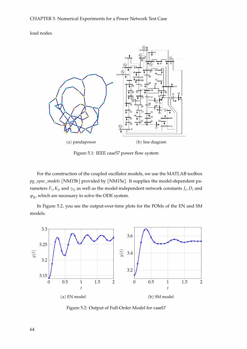
CHAPTER 5. Numerical Experiments for a Power Network Test Case
load nodes.
(a) pandapower (b) line diagram
Figure 5.1: IEEE case57 power flow system
For the construction of the coupled oscillator models, we use the MATLAB toolboxpg_sync_models [NM15b] provided by [NM15a]. It supplies the model-dependent pa-rameters Fi, Kij and γij as well as the model-independent network constants Ji, Di andϕR, which are necessary to solve the ODE system.
In Figure 5.2, you see the output-over-time plots for the FOMs of the EN and SMmodels.
0 0.5 1 1.5 23.15
3.2
3.25
3.3
t
y(t)
(a) EN model
0 0.5 1 1.5 2
3.2
3.4
3.6
t
y(t)
(b) SM model
Figure 5.2: Output of Full-Order Model for case57
64

5.1. Test Setup and Parameters
Standard Test Parameters5
We solve the ODE systemwith a Runge-Kutta-4 scheme using step size h = 0.001 as thestandard for the BT tests, and ode45 as the standard for the POD tests6.
The standard time interval is T = [0; 2], because the assumptions for the COmodelsare only valid for short time scales7 [NM15a]. To illustrate the convergence behavior ofthe ROM output, we also look at a longer time interval of T = [0; 10].
The standard choice for the mathematical CO ODE system representation is thequadratic system in matrix version (4.9).
We test two initial values, where δ0 ∈ {0, π}, and two output matrices: C1st , (4.15),the output of the first oscillator’s phase angles, and Cam, (4.16), the arithmetic mean ofthe phase angles. This makes four (δ0, C) testing pairs. The standard choice is (π, C1st).
Table 5.1 provides an overview of those tested parameters that are not influencedby the choice of the CO model.
Table 5.1: Model-Independent MOR Parameters for case57
standard also tested
test case PN case57 –# generators ng 7 –# nodes n 57 –ODE solver Runge-Kutta-4 ode45 for PODtime interval T [0; 2] [0; 10]
shift α 0.05 [0, 0.5] with step size 0.01
(δ0, C) (π, C1st) (π, Cam), (0, C1st), (0, Cam)
The start and step values of the reduction order nρ depend on the COmodel. Thereis no standard choice for the latter parameter. Throughout the numerical experiments,we vary nρ.
Concerning the BT-specific parameters, there are three main values which can bemodified: the number of Volterra kernels ν, and the α shift of matrix A, i.e., Aα. In someinstances, the method is tested with different numbers of Volterra kernels, ν ∈ {1, 3, 5},with the standard choice of ν = 3. We abbreviate BTwith 1, 3 and 5Volterra kernelswithBT1, BT3 and BT5, respectively. We examine α-shifts ranging between 0 and 0.05 witha step size of 0.01, selecting α = 0.05 as the standard. As mentioned in Section 4.4, the
5When not otherwise mentioned, we tested with the parameters denoted as standard.6When we started, we also used the Runge-Kutta-4 scheme for the POD tests. When during testing
some re-programming was necessary for the POD method, it was more convenient to switch to ode45.Since the Runge-Kutta-4 scheme is just as accurate as the ode45 solver for the BT method, this has noinfluence on the results.
7See, e.g., the assumptions for the classical model on Page 9.
65

CHAPTER 5. Numerical Experiments for a Power Network Test Case
shift only affects the computation of the projection matrices. The actual ODEs systemis solved with the unshifted matrix A.
For our naive implementation of the POD method, there is only one adjustable pa-rameter: the number of snapshots ζ. As discussed in Section 3.4, there is no rule whatsize ζ should be in general. The goal is to use as few snapshots as possible but as manyas necessary8. Sample experiments showed that once a certain threshold of snapshotsis reached, increasing the number of snapshots does not improve the performance.
In Table 5.2 you can find the test parameters which depend on the the selected COmodel.
Table 5.2: Model-Dependent MOR Parameters for case57
EN model SM model
red. order nρ start 4 8red. order nρ step 4 10red. order nρ end 24 218size FOM (4nco) 28 228size 1st-ord. sys. nmin 14 114# snapshots ζ 981 4333
Evaluation Measures
We examine three measures overall:
(i) output behavior y(t),
(ii) singular values σ,
(iii) L∞ error.
Considering the first item, this is simply an output-over-time plot. As we statedin Remark 4.5, we used the nonzero transformed system (4.21) to solve the ROM aswell as the FOM. So, we plot y(t) = Cx(t) + Cx0 and y(t) = Cx(t) + Cx0 for t ∈ T.This direct comparison of the outputs for the FOM and ROM provides an intuition ofthe approximation quality and helps to assess the L∞ approximation error, the thirdevaluation measure.
8We employed the formula ζ = βn2co + 1, where β = 20 for the ENmodel, and β = 4
3 for the SMmodel.This model-dependent factor is doubled, if the POD should fail due to too few snapshots. The snapshotfactor β made it easier during programming to scale the number of snapshots ζ. Computing the time stepdistances T
ζ , then starting to the build the snapshot matrix at t0 = 0 and ending at tζ = T adds 1 to thenumber of snapshots
66

5.1. Test Setup and Parameters
Specifically, in Section 5.2, we look at the output-over-time for BT3 with time inter-vals T = [0; 2] in Figure 5.3, and T = [0; 10] in Figure 5.4, as well as for PODwith a timeinterval of T = [0; 10] in Figure 5.5.
Concerning the second measure, in Section 5.5, we look at the SVs of the Grami-ans, the Hankel SVs (computed with Algorithm 3.3) in Figure 5.9, and the SVs of thesnapshot matrix X (computed with Algorithm 3.4). We actually examine the X -SVs’behavior not only for the snapshot matrix of the quadratic system (4.9), but in additionthe SVs for the snapshot matrix of the 1st-order nonlinear system (4.3)9 in Figure 5.10.
In our evaluation, the SVs are normalized such that the largest SV is 1, i.e.,
σ =σ
||σ|| .
We evaluate two features by measuring the third item, the absolute L∞ error. First,we examine the distance between the FOM output y(t) and the ROM output y(t), thatis,
ε∞ = ||y(t)− y(t)||L∞ = maxt∈T
|y(t)− y(t)|, (5.1)
for which we use the MATLAB norm function. We look at this measure in our cross-method comparison of the output error in Section 5.3, for the time interval T = [0; 2] inFigure 5.6 and for the time interval T = [0; 10] in Figure 5.7. We also evaluate the mea-sure for BT3 when we compare the combinations of different initial values and outputmatrices in Section 5.6 in Figure 5.11. It is used, too, to investigate the influence of the α
shift value in Section 5.7, again for BT3 in Figure 5.12.
Second, we also look at the L∞ error of the PTI, i.e., we check if
s2(t) + c2(t) = 1,
holds, where s, c ∈ R4nco are the sine and cosine components (4.10) of the pulled backand back-transformed state vector x = Vα x + x0 as described at the end of Section 4.4on Page 61. Using MATLAB’s max function, we first compute
ε./∞ = ||(s2(t) + c2(t))− 1||L∞ = maxt∈T
((s2(t) + c2(t))− 1), (5.2)
which gives us an absolute L∞ error estimate for each oscillator. If ε./∞ > 103, the erroris considered to be ε./∞ = ∞. We then select the best and worst performing oscillatorbased on the mean ε./∞ value across reduction orders nρ. If there are Inf or NaN values,we set them to 107, but only for the computation of the mean, such that if there are Infor NaN values, you can “spot” them by their absence in the plots without distorting the
9The unlifted system is only half as large as the quadratic system. However, because this system lacksstructure, the nonlinear terms must be estimated by other techniques, termed “hyper-reduction”. Thisprovokes a second approximation of the system and can become costly, depending on the degree of non-linearity in the system. As [KW19] note, the lifted system representation is not unique but exact, i.e., thereis no extra approximation necessary. POD can be directly applied to the lifted system and exploit the addedstructure.
67

CHAPTER 5. Numerical Experiments for a Power Network Test Case
curve. We choose the two oscillators per MOR method with maximum and minimummean. Investigating the PTI is another means to evaluate the quality of the MOR. Anadvantage is the identity’s independence of the choice of the outputmatrix. We examinethis measure in Section 5.4 for BT1, BT3, BT5 and POD in Figure 5.8.
To improve interpretability, all SVs σ and both L∞ errors, ε∞ and ε./∞ , are plotted ona logarithmic scale.
Before we evaluate the test results, we need to keep two things in mind: First, wequadruple the size of the CO models by lifting them to quadratic form. However, sincewe want to solve the ODE system by numerical software, we would have to doublethe original size of nco anyway to transform the 2nd-order ODE systems of size nco to a1st-order ODE systems. We therefore define
nmin = 2nco, with nENmin = 14, and nSM
min = 114, (5.3)
the minimum size of the system such that it can be solved by numerical software. Sec-ond, we simultaneously want a low reduction order nρ and a small L∞ error. Relatingthis to the first reminder, we may consider a MOR a success, if we have an acceptableL∞ error and nρ < nmin is valid for the associated reduction order.
Furthermore, we point out that the balancing and truncating parts of BT in principleworked in all tests10. When we declare that a BT method “failed” or did “not work”or the like in the following sections, we do not mean that the method itself could notbe performed, but that the subsequent solution of the ODE system based on the BTreduction failed to produce a computable error, i.e., an error that did not result in Inf orNaN. The only exception is the examination of the α-shift influence, which we discussin Section 5.7.
In our analysis of the evaluation items, we always start by examining Balanced Trun-cation (and its versions, where applicable), first for the EN, second for the SM model,then we make a cross-model comparison, and eventually contrast the findings with theperformance of Proper Orthogonal Decomposition (POD).
5.2 Proof-of-Concept: Output-over-Time Behavior
We begin our evaluation by examining the output-over-time for different reduction or-ders nρ in Figures 5.3 and 5.4 for BT3, and Figure 5.5 for POD.
EN Model: We see in Figure 5.3a that the output for the first three reduction or-der values nρ ∈ {4, 8, 12} diverges from the FOM output already in the 2 seconds in-terval. As we move to the 10 seconds interval in Figure 5.4a, we omit these reduction
10However, whenever the Cholesky factors of the Volterra kernels and/or Gramians were computedwith Algorithm 3.2 (and Algorithm C.1), it was almost always necessary to approximate the respectivematrix with an symmetric positive definite (SPD) matrix (see Appendix C).
68

5.2. Proof-of-Concept: Output-over-Time Behavior
× full nρ = 4 nρ = 8 nρ = 12
nρ = 16 nρ = 20 nρ = 24
0 0.2 0.4 0.6 0.8 1 1.2 1.4 1.6 1.8 2−8
−6
−4
−2
0
2
4
t
y(t)
(a) EN model
× full nρ = 8 nρ = 18 nρ = 28
nρ = 38 nρ = 48 nρ = 58 nρ = 68
nρ = 78 nρ = 88 nρ = 98 nρ = 108
nρ = 118 nρ = 128 nρ = 138 nρ = 148
nρ = 158 nρ = 168 nρ = 178 nρ = 188
nρ = 198 nρ = 208 nρ = 218
0 0.2 0.4 0.6 0.8 1 1.2 1.4 1.6 1.8 23.1
3.2
3.3
3.4
3.5
3.6
3.7
t
y(t)
(b) SM model
Figure 5.3: Output of BT3
69

CHAPTER 5. Numerical Experiments for a Power Network Test Case
× full nρ = 20 nρ = 24 nρ = 24
0 2 4 6 8 103.1
3.15
3.2
3.25
3.3
3.35
3.4
t
y(t)
(a) EN model
× full nρ = 68 nρ = 78 nρ = 88
nρ = 98 nρ = 108 nρ = 118 nρ = 128
nρ = 138 nρ = 148 nρ = 158 nρ = 168
nρ = 178 nρ = 188 nρ = 198 nρ = 208
nρ = 218
0 2 4 6 8 103.1
3.2
3.3
3.4
3.5
3.6
3.7
t
y(t)
(b) SM model
Figure 5.4: Output of BT3 for 10s Interval
70

5.2. Proof-of-Concept: Output-over-Time Behavior
orders and in addition nρ = 16 to avoid distortion. For almost 3 seconds, the output forthe remaining orders stays relatively close to the FOM output. Nonetheless, after thattime instance, the output of the EN model for the remaining two reduction orders alsobranches out.
SM Model: The SM model in Figure 5.3b looks a little more promising. A higherproportion of reduction orders seems to produce output which stays within a shortdistance of the FOM output. However, some of the lower reduction orders generatedinteresting output behavior. The output for nρ = 8 looks linear. The lines relating tonρ ∈ {18, 28, 38, 48, 58} demonstrate an almost inverse development between 0.6 and 1.4
seconds, after staying close to the FOM output for the first 0.3 seconds. The latter is alsotrue for the output line of nρ = 68. Subsequently, it mimics an upwards shifted FOMoutput.
Analogously to the EN model, we eliminate these worst reduction orders to get aclearer picture in Figure 5.4b. After the omission only the outputs relating to nρ > 68
are left. In the first 3 seconds the output for these orders keep close to the FOM output;except the output for nρ = 68, which retains its shifted progression during this time.Until the end of the 10 seconds interval, however, output for nρ = 68 diverges almost asmuch as the one for nρ = 78. In contrast, the output for nρ = 88 seems to approximatethe FOM well, while the output related to nρ ∈ {98, 108, 118, 128, 138, 148, 158, 168} de-viates noticeably. This leaves only output produced by reduction orders nρ > 178withinimperceptible distance of the FOM output.
ENvs. SMModel: FromFigure 5.3, we discern that BT3 does not accomplish a goodapproximation of the FOM for low- to mid-range reduction orders regarding both COmodels. In the standard time interval of 2 seconds, the EN model output only stayedclose to the FOM for reductions orders nρ > 16 > nEN
min = 14. The reduction perfor-mance of SM is better, considering nSM
min = 114 in the same interval. The four outputlines relating to reduction orders between 78 6 nρ 6 108 satisfy nρ 6 nSM
min = 114 andseem to progress near the FOM output.
We compare the observations concerning the output with the L∞ output error inSection 5.3, before we draw more conclusions on the performance of BT3.
BT3 vs. POD: We focus immediately on the plot with a time interval of T = [0; 10]
in Figure 5.5 and compare the findings thus far to the output approximations achievedby POD. Evidently, this MORmethod’s output aligns with the FOM output already forreduction orders of nρ > 12 for the EN model in Figure 5.5a, with nρ = 8 also seemingwithin reasonable distance. POD performs even better for the SMmodel in Figure 5.5b.Merely for nρ = 8, the reduced output oscillates with larger distance around the actualoutput values. All other reduction orders seem to immediately align with the full-orderoutput11. So, judging by the output behavior, the POD performance is more accurate
11One aspect to point out is that the produced output for nρ = 8 does not start at y(0) = π which
71

CHAPTER 5. Numerical Experiments for a Power Network Test Case
× full nρ = 4 nρ = 8 nρ = 12
nρ = 16 nρ = 20 nρ = 24
0 2 4 6 8 103.14
3.16
3.18
3.2
3.22
3.24
3.26
3.28
3.3
t
y(t)
(a) EN model
× full nρ = 8 nρ = 18 nρ = 28
nρ = 38 nρ = 48 nρ = 58 nρ = 68
nρ = 78 nρ = 88 nρ = 98 nρ = 108
nρ = 118 nρ = 128 nρ = 138 nρ = 148
nρ = 158 nρ = 168 nρ = 178 nρ = 188
nρ = 198 nρ = 208 nρ = 218
0 2 4 6 8 103.1
3.2
3.3
3.4
3.5
3.6
3.7
t
y(t)
(b) SM model
Figure 5.5: Output of POD for 10s Interval
72
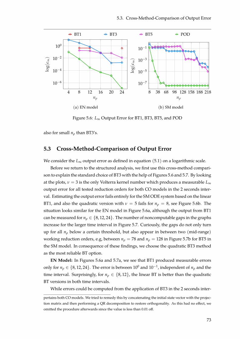
5.3. Cross-Method-Comparison of Output Error
◦ BT1 ◦ BT3 ◦ BT5 ◦ POD
4 8 12 16 20 24
10−6
10−4
10−2
100
nρ
log(
ε ∞)
(a) EN model
8 38 68 98 128 158 188 218
10−7
10−5
10−3
10−1
nρ
log(
ε ∞)
(b) SM model
Figure 5.6: L∞ Output Error for BT1, BT3, BT5, and POD
also for small nρ than BT3’s.
5.3 Cross-Method-Comparison of Output Error
We consider the L∞ output error as defined in equation (5.1) on a logarithmic scale.Before we return to the structured analysis, we first use this cross-method compari-
son to explain the standard choice of BT3with the help of Figures 5.6 and 5.7. By lookingat the plots, ν = 3 is the only Volterra kernel number which produces a measurable L∞
output error for all tested reduction orders for both CO models in the 2 seconds inter-val. Estimating the output error fails entirely for the SMODE system based on the linearBT1, and also the quadratic version with ν = 5 fails for nρ = 8, see Figure 5.6b. Thesituation looks similar for the EN model in Figure 5.6a, although the output from BT1can bemeasured for nρ ∈ {8, 12, 24}. The number of noncomputable gaps in the graphsincrease for the larger time interval in Figure 5.7. Curiously, the gaps do not only turnup for all nρ below a certain threshold, but also appear in between two (mid-range)working reduction orders, e.g, between nρ = 78 and nρ = 128 in Figure 5.7b for BT5 inthe SM model. In consequence of these findings, we choose the quadratic BT3 methodas the most reliable BT option.
EN Model: In Figures 5.6a and 5.7a, we see that BT1 produced measurable errorsonly for nρ ∈ {8, 12, 24}. The error is between 100 and 10−1, independent of nρ and thetime interval. Surprisingly, for nρ ∈ {8, 12}, the linear BT is better than the quadraticBT versions in both time intervals.
While errors could be computed from the application of BT3 in the 2 seconds inter-
pertains both COmodels. We tried to remedy this by concatenating the initial state vector with the projec-tion matrix and then performing a QR decomposition to restore orthogonality. As this had no effect, weomitted the procedure afterwards since the value is less than 0.01 off.
73
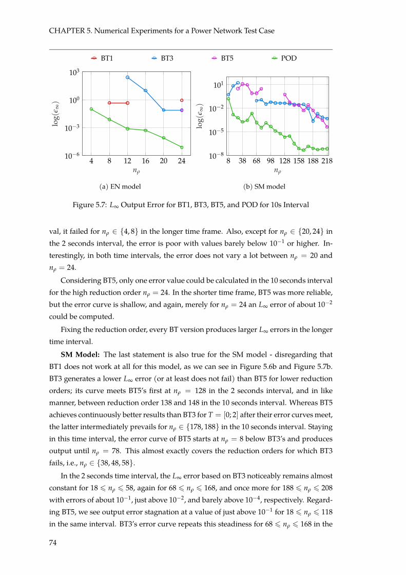
CHAPTER 5. Numerical Experiments for a Power Network Test Case
◦ BT1 ◦ BT3 ◦ BT5 ◦ POD
4 8 12 16 20 2410−6
10−3
100
103
nρ
log(
ε ∞)
(a) EN model
8 38 68 98 128 158 188 21810−8
10−5
10−2
101
nρ
log(
ε ∞)
(b) SM model
Figure 5.7: L∞ Output Error for BT1, BT3, BT5, and POD for 10s Interval
val, it failed for nρ ∈ {4, 8} in the longer time frame. Also, except for nρ ∈ {20, 24} inthe 2 seconds interval, the error is poor with values barely below 10−1 or higher. In-terestingly, in both time intervals, the error does not vary a lot between nρ = 20 andnρ = 24.
Considering BT5, only one error value could be calculated in the 10 seconds intervalfor the high reduction order nρ = 24. In the shorter time frame, BT5 was more reliable,but the error curve is shallow, and again, merely for nρ = 24 an L∞ error of about 10−2
could be computed.
Fixing the reduction order, every BT version produces larger L∞ errors in the longertime interval.
SM Model: The last statement is also true for the SM model - disregarding thatBT1 does not work at all for this model, as we can see in Figure 5.6b and Figure 5.7b.BT3 generates a lower L∞ error (or at least does not fail) than BT5 for lower reductionorders; its curve meets BT5’s first at nρ = 128 in the 2 seconds interval, and in likemanner, between reduction order 138 and 148 in the 10 seconds interval. Whereas BT5achieves continuously better results than BT3 for T = [0; 2] after their error curvesmeet,the latter intermediately prevails for nρ ∈ {178, 188} in the 10 seconds interval. Stayingin this time interval, the error curve of BT5 starts at nρ = 8 below BT3’s and producesoutput until nρ = 78. This almost exactly covers the reduction orders for which BT3fails, i.e., nρ ∈ {38, 48, 58}.
In the 2 seconds time interval, the L∞ error based on BT3 noticeably remains almostconstant for 18 6 nρ 6 58, again for 68 6 nρ 6 168, and once more for 188 6 nρ 6 208
with errors of about 10−1, just above 10−2, and barely above 10−4, respectively. Regard-ing BT5, we see output error stagnation at a value of just above 10−1 for 18 6 nρ 6 118
in the same interval. BT3’s error curve repeats this steadiness for 68 6 nρ 6 168 in the
74

5.3. Cross-Method-Comparison of Output Error
10 seconds time frame with error values a little larger than in the shorter time interval.
EN vs. SMModel: With BT3 and BT5, the reduction accomplishes lower L∞ errorsin the SM model than in the EN model. Even though BT1 worked for some reduc-tion orders in the latter model, the error is so large that the application of this linearversion still seems pointless. Taking only the reduction orders into account for whichnρ 6 nSM
min = 114 holds, at least BT3 produces acceptable results in both time frames forthe SM model assuming an L∞ output error of just above 10−2 is tolerable.
Output-over-Time vs. Output Error regarding BT3: We interpret the findings ofSection 5.2 concerning the output-over-time plots based on the application of BT3 inFigures 5.3 and 5.4 with regard to what we have learned from the L∞ error plots inFigures 5.6 and 5.7.
Considering the EN model first, the blue L∞ error curves confirm the diverging be-havior for nρ ∈ {4, 8, 12} in Figure 5.3awith an L∞ error above or close to 1 in Figure 5.6afor the 2 seconds time interval. For the two smallest reduction orders regarding thelonger time interval, BT3-based ODE solutions failed completely to compute an error< ∞ in Figure 5.7a. The outputs for nρ ∈ {16, 20, 24} look close to the FOM one andthe error curves with values below 10−1 for nρ = 16 and 10−3 for the higher reductionorders support this for the 2 seconds time interval. The L∞ error value of well above101 for nρ = 16 in the 10 seconds time interval also attests that this reduction orderwas rightfully omitted in the longer output-over-time plot to prevent distortions. Theerrors corresponding to nρ ∈ {20, 24} in the longer time intervals likewise corroboratethe growing deviation of the respective output curves with values approximating 10−1.
The findings for the output-over-time plots match those for the L∞ error concerningthe SM model, too. Considering the 2 seconds time interval in Figure 5.6b, the errorfor nρ = 8 borders on 1 and the corresponding output “curve’s” straight progressionmatches this large error in Figure 5.3b. We identified three sets of reduction ordersfor which the L∞ output error stagnated in the same time interval. The first set withreduction orders between 18 and 58 result in an L∞ error of about 10−1. Comparing thiswith the output-over-time, we see their behavior differs a lot from the FOM curve. For68 6 nρ 6 168 the error remains almost stationary just above 10−2. This agrees with theoutput-over-time plot in Figure 5.3b, in which corresponding lines are close together.Reduction order nρ = 68 produces the aforementioned slightly upwards shifted curve,reflecting the comparatively slightly larger output error. The lines corresponding tothe third set of stagnating reduction orders, 188 6 nρ 6 208 can hardly be told apartfrom the FOM output mirroring the small output error of approximately 10−4. Thelarge error values for the first three reduction orders of above 100 and the altogethermissing error values in the 10 seconds time frame match the deleted output-over-timelines in Figure 5.4b. The stagnating output error curve corresponding to 68 6 nρ 6 168
agrees with the slowly growing distance between the related output-over-time lines
75

CHAPTER 5. Numerical Experiments for a Power Network Test Case
4 best, BT1 5 worst, BT1 4 best, BT3 5 worst, BT34 best, BT5 5 worst, BT5 4 best, POD 5 worst, POD
4 8 12 16 20 2410−10
10−6
10−2
102
nρ
log(
ε./ ∞)
(a) EN model
8 38 68 98 128 158 188 21810−12
10−8
10−4
100
nρ
log(
ε./ ∞)
(b) SM model
Figure 5.8: L∞ PTI Error for BT1, BT3, BT5, and POD
and the FOM line. The increase is a little faster for nρ ∈ {68, 78, 98}, reflecting theirslightly larger L∞ error. A surprise is the absolute minimum error value of about 10−4
for nρ = 188.In Figure 5.4, we could already see the progressing divergence of the output-over-
time lines, especially for the EN model. This indication that reduction by BT3 might beuseful for short time intervals, but grows more unreliable with time, is substantiatedby the L∞ output error. In both CO models, the error is either high or not computablefor low reduction orders. For mid-range to high reduction orders, we observe the errorgrows larger in time. Comparing the output error in the 2 seconds intervalwith the errorin the 10 seconds interval for fixed nρ value, we notice a greater difference between theerrors in the EN than in the SM model.
BT vs. POD: Regardless of CO model and time frame, POD always outperformsthe BT approaches. Its green error curves have a much steeper development, especiallyfor the SM model, the method achieves much lower errors, and works for all reductionerror in all time intervals. These findings coincide with the findings in Section 5.2.
5.4 Cross-Method-Comparison of Pythagorean TrigonometricIdentity Error
In Figure 5.8, we look at the L∞ PTI errors of the best and worst oscillators as derived inSection 5.1 on Page 67 and the error defined there in equation (5.2). We also examinehow this error compares with L∞ output error of the respective model and MOR ap-proach. Note, that we only consider the standard time interval of T = [0; 2] from nowon.
76

5.4. Cross-Method-Comparison of Pythagorean Trigonometric Identity Error
EN Model: First addressing BT1 in Figure 5.8a, determining the L∞ PTI error wasnot successful. Theworst oscillator offers only twousable errors for the reduction ordersof 8, 12 with a large value of above 10. They are higher than the respective L∞ outputerrors in Figure 5.6a. There is also only a single error with a value just below 10−1, atnρ = 24, belonging to the best oscillator. It is, however, smaller than the correspondingL∞ output error. BT1 performs worst of the tested MOR methods.
Next considering BT3, this is a good illustration that small differences in values canappear large on a logarithmic scale. We observe that the curves of the best and worstoscillator are nearly identical for the lowest three reduction orders, nρ ∈ {4, 8, 12}, andwithin short distance for the next two, nρ ∈ {16, 20}. That the worst oscillator’s errorcurve does not only steeply decrease in contrast to the best oscillator’s curve for nρ = 24,but it also undercuts the L∞ output error for the same reduction order. In general, how-ever, the L∞ PTI error of both curves is worse than the L∞ output error.
Looking at BT5, its curves of the L∞ PTI error show a more shallow progressioncompared to BT3. Nevertheless, the error values are about the same or even lower thanBT3’s – exempting the missing values for nρ = 4 (best and worst), and nρ ∈ {20, 24}(best only). We observe that BT5’s worst and best oscillator error curves are very closefor nρ ∈ {8, 12, 16} with error values falling from around 10−1 to 10−3 for the best andfrom 10−1 to 10−2 for the worst oscillator. With this reduction order set, the L∞ PTIerrors are smaller than the L∞ output errors. There are no best values for the two re-maining reduction orders, but the L∞ PTI error values belonging to the worst oscillatorremain between 10−1 and 10−2, with the one corresponding to nρ = 20 smaller and theone corresponding to nρ = 24 larger than the respective L∞ output error.
SM Model: In Figure 5.8b, we notice that BT1 again does not work at all for thismodel.
At just about every point, the BT3’s worst L∞ PTI error curve is above the L∞ outputerror curve. With the few exceptions of nρ = 8 and nρ > 188, this line almost mimicsthe L∞ output error curve in Figure 5.6b with a slight upwards shift. We recognize twoof the stationary segments, 18 6 nρ 6 58 and 68 6 nρ 6 168, before a rapid decreasein error. Even the minimum at nρ = 188 exists. With an error value of about 10−6, it ismuch lower than its output error counterpart. The L∞ PTI error curve created by thebest oscillator remains close to the worst one until nρ = 68 and then rapidly falls off,before likewise steadying for 98 6 nρ 6 158 with error values between 10−5 and 10−4.Following a slow decrease in error, this curve reaches its minimum at nρ = 188, too.Afterwards, it approximates the line belonging to the worst oscillator.
While BT5 only failed for nρ = 8 concerning the L∞ output error in Figure 5.6b, theL∞ PTI curves have gaps for higher reduction orders. Considering the purple curve ofthe worst oscillator, its L∞ PTI errors are much larger than the corresponding L∞ outputerrors until the first break in the curve. Yet, after the break, the L∞ PTI error values are
77

CHAPTER 5. Numerical Experiments for a Power Network Test Case
much lower compared to the respective L∞ output errors. They are also better thanthe best oscillator’s values. Except for the break, the best oscillator’s PTI performance,however, offers error values well below those of the related parts of the L∞ output errorcurve.
EN vs. SM Model: In parallel to the L∞ output error, the EN model admits L∞ PTIerror values computedwith BT1 in contrast to the SMmodel, but they are still scarce andlarge. The reduction by BT3 and BT5 in the SM model results in smaller L∞ PTI errorsfor the best oscillators, too, compared to the other COmodel. Their best andworst errorcurves have a greater distance than in the ENmodel, especially for mid-range reductionorders.
Again, solely allowing for reduction orders with nρ 6 nENmin = 14 for the EN model,
and nρ 6 nSMmin = 114 for the SM model, respectively, BT5 alone might be considered to
provide a tolerable L∞ PTI error with values between 10−1 and 10−2 for both best andworst oscillator. Regarding the SM model, only the best oscillators’ error curves havesmaller error values than 10−1. BT5’s best oscillator curve satisfies this error thresholdfor all reduction orders 18 6 nρ 6 108 6 nSM
min = 114, while BT3’s error values complywithin the range 78 6 nρ 6 108 6 nSM
min = 114
BT vs. POD:Once again, POD outperforms BT. For most of the reduction orders inboth CO models, there is a huge distance between the L∞ PTI errors produced by theMOR reduction and the BT approaches. In addition, all of POD errors are small, evenfor nρ = 4 in the ENmodel, and nρ = 8 for the SMmodel, the values are comparativelylow.
5.5 Evolution of the Singular Values
In this section, we first look at the BT3-related SVs in Figure 5.9. We then comparethe SVs of POD’s snapshot matrices for the lifted quadratic system (4.9) and the trans-formed 1st-order ODE system (4.3) in Figure 5.10. Afterwards, we contrast BT3 andPOD.
EN vs. SM Model: As characterized in Definition 3.22 and stipulated in Lemma3.23, the Hankel SVs and the SVs of the reachability and observability Gramians, Pand Q, should be equal in a (principal-axis) balanced system. Figure 5.9 depicts thatthis does not hold for both CO models in our case. In contrast, the three SV curvesin each plot show a pronounced difference. A common trait is the sharp decrease forthe first SVs, and the subsequent preliminary stagnation. This first stationary segment(although on different levels for the different SV types) sets in before our first testedreduction order value nρ = 4 for EN, and nρ = 8 for SM model. So, testing even lowerorders would probably not have been successful.
Focusing on theHankel SV curve, we observe that the first stagnation ends at aroundthe 12th Hankel SV in the EN model, and shortly before the 68th Hankel SV in the SM
78

5.5. Evolution of the Singular Values
◦ log(σHankel) log(σP ) log(σQ) nρ = 24
4 8 12 16 20 24 2810−12
10−8
10−4
100
number of σ
log(
σ)
(a) EN model
8 38 68 98 128 158 188 21810−10
10−7
10−4
10−1
number of σ
log(
σ)
(b) SM model
Figure 5.9: Hankel SVs, and SVs of Gramians P ,Q
model. The former CO model has two additional stationary phases between the 16th
and 20th, and the 21st and 26th Hankel SV. The SM model has only one additional stag-nant segment starting around the 68th and ending at circa the 158th Hankel SV. Theremainder of the Hankel SV curve slowly decreases until Hankel SV 218, and then fallsof sharply. If we highlighted the Hankel SV numbers which are also in our set of testedreduction orders, the evolution of the Hankel SVs mimics the progress of the L∞ out-put error in Figure 5.6 for both CO models. Especially, the L∞ output error stagnationintervals for the SM model are retraceable.
Taking also the SVs of the Gramians into consideration, we see that for the mostpart, the Hankel SVs are larger than or equal to the SVs of the Gramians and they do notdecrease as much. Whereas the SV curves of the Gramians cross several times in the ENmodel, the line belonging to the observability Gramian is always above the reachabilityone in the SM model. In general, the SVs in the EN model are smaller compared to theother model.
Lifted vs. Unlifted ODE System: Figure 5.10 depicts the decline of the SVs of thesnapshot matrices for the lifted quadratic ODE system (4.9) and the unlifted 1st-ordernonlinear ODE system (4.3). The two respective curves in the EN and SM model plotsfall off fast, even more so for first SVs in the latter model. The lines are actually alignedfor the prime 10 SVs, and the 25 SVs, respectively. After that, the curves belongingto the unlifted system accelerates its decrease. Nonetheless, the SVs belonging to thelifted quadratic system decay rapidly, too. This implies that the projection matricescomputed from the SVD of the unlifted and lifted snapshot matrix, respectively, spanthe same or at least a very similar low-dimensional subspace in which the state vectorcan be approximated. So, POD does not suffer from the system lifting.
We can also spot the parallel progression of the quadratic system’s snapshot SV
79

CHAPTER 5. Numerical Experiments for a Power Network Test Case
lifted unlifted
0 10 20 3010−10
10−7
10−4
10−1
number of σX
log(
σX)
(a) EN model
0 50 100 150 200 25010−18
10−12
10−6
100
number of σX
log(
σX)
(b) SM model
Figure 5.10: Singular Values of POD Snapshot Matrices for Lifted Quadratic and Un-lifted Nonlinear System
curve and the L∞ output error as well as the L∞ PTI error curves in Figure 5.6 andFigure 5.8, respectively.
BT3 vs. POD: Focusing on the X -SVs of the quadratic system, we see that their de-scent ismuchmore rapid and lower compared to the fall-off of the BT3-related SVs. Thisexplains the better performance of POD across reduction orders, CO models, and timeframes. Especially juxtaposing the Hankel SVs with the X -SVs illustrates the former’scomparatively shallow decrease
5.6 Influence of Initial Value &OutputMatrix on Output Error
In Figure 5.11, we inspect the L∞ output error for four combinations, i.e., four pairs(δ0, C) of two initial values and two output matrices as mentioned in Section 5.1 andsummarized in Table 5.1 on Page 65.
EN Model: For nρ = 4, the BT reduction does not work at all for the pair (0, C1st),but the L∞ output errors for the other combinations are comparatively close. The pair(0, C1st) negatively diverges, and the pair (0, C1st) starts with a large error value of 102
at nρ = 8, while having a very similar (large) error. The error curves of all pairs arealmost aligned for reduction orders nρ > 12.
SM Model: Regarding the SM model, two features stand out: First, both pairs in-cluding output matrix Cam almost always perform better than the other two. Second,there is almost no improvement in the output error in the reduction order sets we iden-tified in Section 5.3 for all combinations.
EN vs. SM Model: Although the curves develop a little erratically for nρ < 12 inthe EN model, and the two curves relating to the (δ0, Cam) pairs have a negative shift,the L∞ output error behavior is very similar in both COmodels in general. Considering
80

5.7. Influence of α-Shift on Output Error
(0, C1st) (0, Cam) (π, C1st) (π, Cam)
4 8 12 16 20 24
10−2
100
102
nρ
log(
ε ∞)
(a) EN model
8 38 68 98 128 158 188 21810−5
10−4
10−3
10−2
10−1
100
nρ
(b) SM model
Figure 5.11: L∞ Output Error for (δ0, C) pairs of Initial Values and Output Matrices
our previous findings, this supports the assertion that the evolution of the Hankel SVsis more important to the BT reduction result than the decision on a particular initialvalue or output matrix.
We chose the pair (π, C1st) as standard, because the output of one oscillator is easierto interprete than the average of all, and we wanted an initial value that is also nonzerofor the 1st-order ODE system.
5.7 Influence of α-Shift on Output Error
In this section, we examine to what extent the choice of the α-shift to makematrix A sta-ble affects the L∞ output error performance of BT. To that end, we examine the heatmapsin Figure 5.12, depicting the error value on a color scale for α values between 0 and 0.5
with a step size of 0.01 and the usual reduction orders.EN Model: For α = 0, BT3 itself does not work. Without a shift, A violated the
requirement for a stable matrix in Definition 3.14, and therefore the assumption for astable system in Theorem 3.15, that all its EVs must be in the left half of the complexplane. In consequence, neither the Lyapunov-Cholesky routine in Algorithm 3.1 northe Gramians in Algorithm 3.2 and Algorithm C.1 could be computed.
This was not the reason for the other white cells in the heatmap for reduction ordersnρ = 8 and especially nρ = 4. Here, the error computation resulted in NaN.
An evident finding is that for high reduction orders nρ ∈ {20, 24}, all tested α valuesresulted in output errors of 10−2.5 or smaller. In contrast, discovering a pattern betweenα value and output error for the other reduction orders is more difficult. There is nonρ for which the output error progresses downwards on the color scale along with in-
81

CHAPTER 5. Numerical Experiments for a Power Network Test Case
4 8 12 16 20 24 n
0
0.1
0.2
0.3
0.4
0.5
log( )
-3
-2.5
-2
-1.5
-1
-0.5
0
0.5
(a) EN model
8 18 28 38 48 58 68 78 88 98 108
118
128
138
148
158
168
178
188
198
208
218
n
0
0.1
0.2
0.3
0.4
0.5
log( )
-4
-3
-2
-1
0
(b) SM model
Figure 5.12: Impact of Different Aα on L∞ Output Error
creasing alpha, or vice versa. There are also merely a few α values for which the outputerror improves with increasing the reduction order. Order nρ = 16 is especially inter-esting, because it is more sensitive to the shift values than reduction orders nρ = 8 andnρ = 12. It results in worse L∞ output errors for many of the α values compared to thelower reduction orders. It actually works best with α = 0.01, a value which producesthe worst error for nρ = 12. Disregarding the two highest and the lowest reductionorders nρ ∈ {4, 20, 24}, nρ = 12 shows the most coherent behavior, moving from redto light blue with increasing α. But here, too, there are output error values disturbingthe color flow, e.g., for α = 0.05. These anomalies occur for all reduction orders withdifferent frequency, quantity, and significance.
SM Model: Shifting A is likewise absolutely necessary to perform the balancingpart of BT3 concerning this model, for the same reason and reasoning as above. Incontrast to the other CO model, L∞ output errors can be computed for all other shiftand reduction order values.
The error progression appears a little more comprehensible. While for this COmodel, too, color distribution follows no stringent pattern, moving from left to rightalong reduction orders, there is a general tendency to encounter lower output errors.Going from top to bottom along α values, however, it is harder to spot a pattern. Forreduction orders nρ > 68, very low α shifts work better than larger ones, especiallyfor nρ > 178, where the output error seems to be inversely proportional to the shiftvalue. It looks as if the exact shift value does not significantly affect the output error for78 6 nρ 6 198 after passing a certain α threshold. In between 128 6 nρ 6 198, thereis a second threshold as we can see a yellow area squeezed in between very small andmid-range α values.
For lower reduction orders nρ 6 58, the L∞ output error is for the most part worse,and the error pattern is also more inconsistent than for higher orders. Both findings can
82

5.7. Influence of α-Shift on Output Error
be inferred from the color distribution.EN vs. SM Model: Both models need a minimum α shift to make BT work. They
also have in common that for a number of reduction orders, very small shifts producebetter results than larger ones. An interpretation is that, depending on the system sizeand the reduction order, on the one hand, α must be large enough to make A stable,and on the other hand, it must not be too large such that the matrix is not shifted toofar from the original.
However, this does not explain the unclear relation between the value of α and theL∞ output error, which ismore pronounced in the ENmodel. Tomake out somepattern,we have to factor in the reduction order. This indicates that the success of BT3 dependsmore on the reduction order than on the shift.
Due to this arbitrary behavior of the shift, we picked the standard value of α = 0.05
for the numerical experiments, reasoning that it was large enough tomake A stable, butsmall enough to keep it close to the original.
83

CHAPTER 5. Numerical Experiments for a Power Network Test Case
84
CHAPTER 6
Summary and Conclusion
The main contribution of this thesis is the application and examination of an only re-cently proposed MOR method – Balanced Truncation adapted from the linear to thequadratic(-bilinear) case – to a problem of practical, real-world importance – the solu-tion of a nonlinear ODE system which models PN dynamics.
We used quadratic lifting of the system, an approach lacking research especially inthe context of MOR. We contributed implementations of the PN ODEmodels given themodel-dependent parameters, such that they can be solved viaMATLAB. This includesthe transformed lifted quadraticmatrix ODE representation towhich quadratic BT (andPOD) can be applied. We derived and implemented the adapted quadratic version ofBT. Its performance was examined by testing the influence of specific, selectable reduc-tion parameters, like the reduction order or the stabilizing shift, and pitched it againstthe well-established POD method.
From these numerical experiments, we draw these main conclusions and proposesome conjectures from our analysis of the CO model MOR by BT:
The application of BT1, i.e., linear BT, to a quadratic system does not give good ap-proximations. While this is probably foreseeable, it might come as a surprise that BT5overall does not perform as good and is not as reliable as BT3, especially for lower reduc-tion orders. Considering that the computation of the Volterra kernels is very costly, it isvaluable to know that adding more kernels does not necessarily help the performance.
The output from the reduced solutions grows unstable for longer time intervals; themagnitude of divergence seems to depend on the underlying CO model or the systemsize. The output divergence and error is greater for the smaller EN model than forthe SM model in any case. Since some of the necessary assumptions to derive the COmodels’ parameters are only valid for short time periods, anyway, this might not be anissue in the reduction of power networks.
In general, the reduction worked better for the latter CO model. This raises thequestion whether BT is better suited for larger systems, or whether the CO model rep-resentation is the crucial factor. It would be interesting to represent other power flowcases as EN and SM models in quadratic structure, and study if the reduction by BTreproduces the findings in a cross-CO-model-test-case comparison. The implementedfunctions and scripts are ready to test different, small power flow cases. The code to
85

CHAPTER 6. Summary and Conclusion
determine the Gramians could also be optimized to study larger systems, e.g., by par-allelization of the bottle-neck Kronecker product, or better memory allocation.
Experiments with varying initial value, output matrix, and shift indicate that thereduction performance depends more on the reduction order and Hankel SV evolutionthan on the specific values of x0, C and α. At all events, the decrease of the Hankel SVsprovides the most reliable measure to predict how successful the BT reduction will be.The comparison of output error andHankel SVs also reveals the link between these SVsand the reduction order.
Overall, the reduction performance of BT is not very satisfactory. This is especiallyevident whenever we measure it against POD. However, POD has the disadvantage ofdepending on a fixed input and the snapshot instances. So, BT might have its advan-tages here, because once the projection matrices are computed, we can just reuse them.Testing modified static or time-dependent inputs would give some insights.
In conclusion, it is too soon for a final verdict on quadratic Balanced Truncation. Thisthesis provides some preliminary results and lays the ground for further experiments.
86

APPENDIX A
More on Gramians, Stability and Energy Functionalsfor Balanced Truncation
A.1 Linear Reachability and Observability Concepts
We consider the system Σ =
(A B
)with A ∈ Rn×n, B ∈ Rn×m.
Theorem A.1 (Reachability properties, [Ant05]).
(1) The reachability space Xreach ⊆ X is a linear space. It holds
Xreach = im(R(A, B)).
(2) AXreach ⊆ Xreach, i.e., the reachable subspace is A-invariant.
(3) Σ is (completely) reachable if and only if rank(R(A, B)) = n.
(4) Reachability is independent of the system basis.
PropositionA.2 (Relation of ReachabilityMatrix andGramian, [Ant05]). For all timest > 0, the column space of the reachability Gramian generates the whole reachability subspace,i.e.,
im(P(t)) = im(R(A, B)).
With respect to the observability concept, we consider the system Σ =
(A
C
)with
A ∈ Rn×n, C ∈ Rp×n.
Theorem A.3 (Observability properties, [Ant05]).
(1) The unobservability subspace Xunobs ⊆ X is a linear space. It holds
Xunobs = ker(O(C, A)) = {x ∈ X |CAi−1x = 0, i > 0}.
(2) AXunobs ⊆ Xunobs, i.e., the unobservable subspace is A-invariant.
(3) Σ is (completely) observable if and only if rank(O(C, A)) = n.
(4) Observability is independent of the system basis.
87

CHAPTER A. More on Gramians, Stability and Energy Functionals for BalancedTruncation
Proposition A.4 (Relation of Observability Matrix and Gramian, [Ant05]). For alltimes t > 0, it holds
ker(Q(t)) = ker(O(C, A)). (A.1)
Employing the duality principle in linear systems, we can show a link between thereachable subspace of a system Σ and the unobservable subspace of its dual system Σ∗.
To that end, we now consider the system (3.3), Σ =
(A B
C
), and define its dual system
as
Σ∗ =
(−A∗ −C∗
B∗
)∈ R(n+m)×(n+p),
with A∗, B∗ and C∗ being the respective dual maps of A, B and C. Their correspondingmatrix representations are the complex transposed matrices A, B and C. The dual sys-tem switches the parts of input and output variables, i.e., −C∗ determines the input, B∗
the output and−A∗ the dynamics of the system. The dual system Σ∗ is also the adjointof Σ with respect to the usual inner product L2(R).
Theorem A.5 (Duality Principle, [Ant05]). It holds:
(XreachΣ )⊥ = Xunobs
Σ∗ .
The system Σ is reachable if and only if its dual Σ∗ is observable.
A.2 Stability
In this section, we consider the autonomous system
x(t) = Ax(t). (A.2)
We present additional definitions and properties concerning stability in order toprovide further information on energy functionals below in Appendices A.3 and A.4.
Definition A.6 (Equilibrium point, [Lue79]). We say x is an equilibrium point of system(A.2) if Ax(t) = 0 for all t > t0. In other words, after the state vector has reached thepoint x, it will stay in that position for all time.
DefinitionA.7 ((Asymptotically) Stable EquilibriumPoint, [Lue79]). LetKx,R be theball of radius R with equilibrium point x at its center.
(i) An equilibrium point x is called stable if for every R > 0 there is an 0 < r < R
such that if x(0) ∈ Kx,r then x(t) ∈ Kx,R for all t > 0.
(ii) An equilibrium point x is called asymptotically stable if in addition to being stablethere is an R > 0 such that if x(0) ∈ Kx,R then x(t) → x for t → ∞.
Aside from the matrix-based system stability in Theorem 3.15, there is also the so-called Lyapunov-based stability, based on a special kind of scalar functions:
88

A.2. Stability
Definition A.8 (Lyapunov Functions, [BG17; Lue79]). A Lyapunov function over a ballK0,r is a continuous function F : Rn → R with continuous first partial derivatives if itholds
(i) F (0) = 0 and F (x) > 0 for x ∈ K0,r \ {0},
(ii) ddtF (x) 6 0 for all x ∈ K0,r.
The first condition attests that, withinK0,r, the functionF (x) is positive definite andhas a unique minimum at x = 0; the second condition means that the gradient of thefunction is negative semidefinite and ensures that the function values are nonincreasingalong all state trajectories within the ball.
Theorem A.9 (Lyapunov Function Stability, [BG17; Lue79]). If there exists a Lyapunovfunction over a ballK0,r, then x = 0 is a stable equilibrium point. If the gradient of the Lyapunovfunction is negative definite for every state vector in K0,r \ {0}, then x = 0 is an asymptoticallystable equilibrium point.
Usually, it is challenging to construct a Lyapunov function, especially for generalnonlinear systems [Lue79], but under linear, autonomous conditions as in system (A.2),we have the well-established quadratic function at our disposal [Ant05]:
F (x) = x∗Px, P = P∗ ∈ Rn×n,
and differentiate the equation to see which properties the function terms must have tomeet the conditions of Definition A.8:
ddtF (x) = x∗Px + x∗Px
= x∗A∗Px + x∗PAx
= x∗ (A∗P + PA)︸ ︷︷ ︸=Z
x
= x∗Zx.
So, to find a suitable P, we need to solve the quadratic Lyapunov function
A∗P + PA = Z. (A.3)
The following theorem establishes the necessary properties of A and Z to ensure theexistence of a unique solution P and the desired system stability behavior.
Theorem A.10 (Lyapunov Equation Stability for Linear Systems, [Ant05]).
(1) If A is stable, then there exists a unique solution P ∈ Rn×n of (A.3) for all Z ∈ Rn×n.
(2) If Z = Z∗, then also P = P∗.
(3) If Z is negative semidefinite and the pair (A, Z) is observable, then P is positive definite.
89

CHAPTER A. More on Gramians, Stability and Energy Functionals for BalancedTruncation
(4) If Z is negative semidefinite and P is positive definite and in addition Z and P satisfy (A.3),then the system (A.2) is stable.
(5) If (4) holds and furthermore (A, Z) is observable, then the system (A.2) is asymptoticallystable.
Considering quadratic systems, the previously givenDefinitionsA.6 andA.8 remainvalid except that we replace the linear autonomous system (A.2) with the quadraticautonomous system
x(t) = Ax(t) + H(x(t)⊗ x(t)
), (A.4)
where x = 0 is a stable equilibrium point [BG17].The Lyapunov method of determining stability is so powerful that we can apply
it to the nonlinear case as well. Even though the analysis of equilibrium points andthe construction of Lyapunov functions is more difficult for nonlinear systems, [BG17]provide the following results (adapted by us for the quadratic case):
Theorem A.11 (Lyapunov Function Stability for Quadratic Systems, [BG17]). Con-sider the quadratic system (3.38) and let A be stable. Furthermore, let the reduced-order system(3.40) be obtained by performing Algorithm 3.3, where low-rank approximations of the trun-cated Gramians are determined by an iterative scheme. Let P1 and Q1 be the solutions to theirrespective linear Lyapunov equations (3.46) and (3.52). We define
r =σmin(V∗GV)
2||Σnρ ||||H||and G = H(2)(P1 ⊗ Q1)(H(2))∗ + C∗C.
Then it holds for the Lyapunov function F (x) = x∗Σx that
F (x) > 0 and ddtF (x) < 0, for all x ∈ K0,r \ {0}, (A.5)
i.e., x = 0 is an asymptotically stable equilibrium point.
A.3 Energy Functionals for Linear Balanced Truncation
In this section, we consider a stable system Σ =
(A B
C
)with A ∈ Rn×n, B ∈ Rn×m and
C ∈ Rp×n.
PropositionA.12 (Computation of Energy FunctionalswithfiniteGramians, [Ant05]).Let the system Σ be reachable and observable and let the finite Gramians P(t),Q(t) be as de-fined in 3.7 and 3.12, respectively. Also, let x =
∫ t0 eA∗(t−τ)Bu dτ and v ∈ im(P(t)) (see
Theorem A.2). Then,||u||2 = x∗P−1(t)x, (A.6)
where u(t) = −B∗eA∗(t−τ)v is the minimal input energy necessary to move the system to thestate x. Furthermore,
||y||2 = x∗0Q(t)x0 (A.7)is the output energy generated by the initial state x0 at time t.
90

A.4. Energy Functionals for Quadratic Balanced Truncation
From the definition of the Gramians, it is clear that
P(t2) > P(t1) and Q(t2) > Q(t1) for t2 > t1,
i.e., the finite Gramians grow larger in time [Ant05]. This also means, using them todetermine the energy functionals is time-dependent.
Remark A.13. The existence, or respectively finiteness, of the energy functionals in Def-inition 3.17 is not always clear. If the system is not stable, Lo can be infinite. By conven-tion, Lc(x0) is infinite if x0 cannot be reached from 0. We therefore assume that bothenergy functionals are finite from now on [Sch93].
A.4 Energy Functionals for Quadratic Balanced Truncation
Wepresent theoremswhich are based on the relaxedDefinition 3.27 of the observabilityenergy functional.
Theorem A.14 (Computation of Energy Functionals of General Nonlinear Systems,[BG17; GM96]). Consider the nonlinear version of system (3.1) with x = 0 as an asymptoti-cally stable equilibrium in two neighborhoodsKo andKc of 0. Assume the system is controllableand observable, and Lo and Lc are smooth functions of x.
(1) For all x ∈ Kc, the controllability energy functional Lc(x) can be uniquely determined bythe partial differential equation
∂Lc
∂xf (x) + f (x)
∂Lc
∂x+
∂Lc
∂xg(x)g∗(x)
∂∗Lc
∂x= 0, Lo(0) = 0, (A.8)
under the assumption there exists a smooth solution Lc on Kc and 0 is an asymptoticallystable equilibrium of −( f (x) + g(x)g∗(x) ∂∗Lc
∂x ) on Kc.
(2) Likewise, for all x ∈ Ko, the observability energy functional Lo(x) can be uniquely deter-mined by the partial differential equation
∂Lo
∂xf (x) +
12
h∗(x)h(x)− 12
µ−1 ∂Lo
∂xg(x)g∗(x)
∂∗Lo
∂x= 0, Lo(0) = −1
2µ, (A.9)
under the assumption there exists a smooth solution Lo onKo and 0 is an asymptotically sta-ble equilibrium of f (x) := ( f (x)− µ−1g(x)g∗(x) ∂∗Lo
∂x ) on Ko with ψ = f (ψ), ψ(0) = x
and µ := −||g∗(ψ) ∂∗ Lo∂x (ψ)||L2 ∈ R.
For the rest of this section, we look at the quadratic system Σ =
(A H B
C
), with
matrices A ∈ Rn×n, H ∈ Rn×n2, B ∈ Rn×m and C ∈ Rp×n.
With the next theorem, [BG17] contribute bounds on the energy functionals usingthe quadratic form of the constructed infinite Gramians. They derive the bounds com-puted with truncated Gramians in Theorem 3.28 from it.
91

CHAPTER A. More on Gramians, Stability and Energy Functionals for BalancedTruncation
Theorem A.15 (Energy Functional Bounds with infinite Gramians, [BG17]).
(1) Let the system be controllable and A be stable. Furthermore, let the reachability GramianP > 0 uniquely satisfy the generalized Lyapunov equation (3.50). Also, using TheoremA.14, let the controllability energy functional Lc(x) be the solution of
∂Lc
∂x(Ax + H(x ⊗ x)) + (Ax + H(x ⊗ x))∗
∂∗Lc
∂x+
∂Lc
∂xBB∗ ∂∗Lc
∂x= 0. (A.10)
Then, there is a neighborhood Kc of 0, such that for x ∈ Kc
Lc(x) >12
x∗P−1x. (A.11)
(2) Let B ≡ 0 and x0 be an initial condition. Let the reachability Gramian P > 0 and the ob-servability GramianQ > 0 uniquely satisfy their respective generalized Lyapunov equation(3.50) or (3.56). Let Lo(x) be the observability energy functional as defined in Definition3.27. Then, there is a neighborhood Ko of 0, such that for x ∈ Ko
Lo(x) 612
x∗Qx. (A.12)
It follows, that the proposed Gramians provide local estimates of the energy func-tionals near the origin.
A strong assumption in Theorems A.15 and 3.28 is the positive definiteness of P .Since this condition often cannot be guaranteed, [BG17] offer a direct connection of theinfinite and truncated Gramians to the reachability and observability of the system. Inconsequence, this ties the proposed Gramians to the classical idea of balanced trunca-tion.
TheoremA.16 (Reachability andObservabilitywith infiniteGramians, [BG17]). Con-sider the system (3.37).
(1) Let the reachability Gramian P > 0 satisfy the generalized Lyapunov equation (3.50). Letthe system be driven from the zero state to x0. If x0 6∈ im(P), then Lc(x) = ∞ for allinputs u.
(2) Let B ≡ 0 and x(0) = x0 be an initial condition. Let the reachability Gramian P > 0 andthe observability Gramian Q > 0 satisfy their respective generalized Lyapunov equation(3.50) or (3.56). If x0 ∈ ker(Q), then the observability energy functional Lo(x0) = 0.
It follows from the first part of the theorem, that a state variable x0 which is not inthe image of P cannot be reached from 0. Conversely, all the states which lie in ker(P)
are uncontrollable. Likewise, the second part asserts that after the elimination of theuncontrollable states (by assuming positive definiteness ofP), the states which are con-tained in ker(Q) are unobservable. Accordingly, states that are in one of the Gramians’kernels are judged unimportant regarding the system’s dynamics. This coupled withthe bounds given in Theorem A.15 correspond with the idea of linear balanced trunca-tion of removing those states with low degrees of reachability and observability, againmeasured by the SVs of the proposed Gramians.
92

A.4. Energy Functionals for Quadratic Balanced Truncation
Corollary A.17 (Reachability and Observability with truncated Gramians, [BG17]).Consider the system (3.37).
(1) Let the truncated reachability Gramian PT and the truncated observability Gramian QT
satisfy the respective Lyapunov equation (3.48) and (3.54). Let the system be driven fromthe zero state to x0 6∈ im(PT ). Then, Lc(x) = ∞ for all inputs u.
(2) Let the quadratic system be locally controllable around 0, and assume that the pair (A, B)
is controllable. Then for B ≡ 0 and x(0) = x0, it holds that if x0 ∈ ker(QT ), thenLo(x0) = 0.
93

CHAPTER A. More on Gramians, Stability and Energy Functionals for BalancedTruncation
94

APPENDIX B
Multi-Linear Algebra Operations
B.1 The Kronecker Product
Let K be either R or C. For a more in depth treatment of the Kronecker product, see[Pol14; ZD13].
Definition B.1 (Kronecker Product, [ZD13]). Let M = [mij] ∈ Kk×` and N ∈ Km×n bematrices. The Kronecker product of M and N is the (km × `n) matrix:
M ⊗ N =[mijN
]
=
m1,1N m1,2N · · · m1,`N
m2,1N m2,2N · · · m2,`N...
... . . . ...mk,1N mk,2N · · · mk,`N
.
Theorem B.2 (Kronecker Product Properties, [ZD13]). Let M ∈ Kk×`, K ∈ K`×p andN ∈ Km×n, L ∈ Kn×r be matrices, and µ a scalar. The following properties hold for theKronecker product:
(1) In general, noncommutativity:
M ⊗ N 6= N ⊗ M.
(2) Linearity in both terms:
M ⊗ (µN) = µ(M ⊗ N) = (µM)⊗ N.
(3) Distributivity and associativity:
(M + N)⊗ K = (M ⊗ K) + (N ⊗ K),
M ⊗ (N + K) = (M ⊗ N) + (M ⊗ K),
(M ⊗ N)⊗ K = M ⊗ (N ⊗ K).
(4) Distributivity of (conjugate) transposition:
(M ⊗ N)∗ = M∗ ⊗ N∗.
95
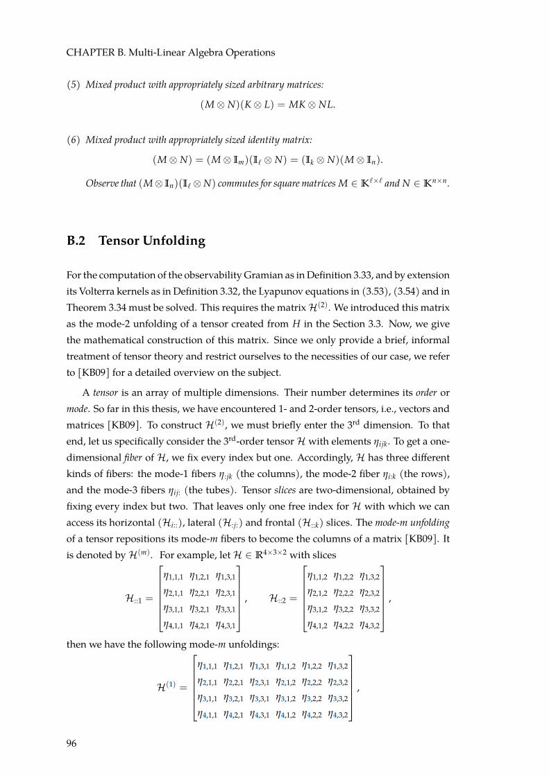
CHAPTER B. Multi-Linear Algebra Operations
(5) Mixed product with appropriately sized arbitrary matrices:
(M ⊗ N)(K ⊗ L) = MK ⊗ NL.
(6) Mixed product with appropriately sized identity matrix:
(M ⊗ N) = (M ⊗ Im)(I` ⊗ N) = (Ik ⊗ N)(M ⊗ In).
Observe that (M⊗ In)(I`⊗ N) commutes for square matrices M ∈ K`×` and N ∈ Kn×n.
B.2 Tensor Unfolding
For the computation of the observability Gramian as inDefinition 3.33, and by extensionits Volterra kernels as in Definition 3.32, the Lyapunov equations in (3.53), (3.54) and inTheorem 3.34 must be solved. This requires the matrixH(2). We introduced this matrixas the mode-2 unfolding of a tensor created from H in the Section 3.3. Now, we givethe mathematical construction of this matrix. Since we only provide a brief, informaltreatment of tensor theory and restrict ourselves to the necessities of our case, we referto [KB09] for a detailed overview on the subject.
A tensor is an array of multiple dimensions. Their number determines its order ormode. So far in this thesis, we have encountered 1- and 2-order tensors, i.e., vectors andmatrices [KB09]. To construct H(2), we must briefly enter the 3rd dimension. To thatend, let us specifically consider the 3rd-order tensor H with elements ηijk. To get a one-dimensional fiber of H, we fix every index but one. Accordingly, H has three differentkinds of fibers: the mode-1 fibers η:jk (the columns), the mode-2 fiber ηi:k (the rows),and the mode-3 fibers ηij: (the tubes). Tensor slices are two-dimensional, obtained byfixing every index but two. That leaves only one free index for H with which we canaccess its horizontal (Hi::), lateral (H:j:) and frontal (H::k) slices. The mode-m unfoldingof a tensor repositions its mode-m fibers to become the columns of a matrix [KB09]. Itis denoted by H(m). For example, let H ∈ R4×3×2 with slices
H::1 =
η1,1,1 η1,2,1 η1,3,1
η2,1,1 η2,2,1 η2,3,1
η3,1,1 η3,2,1 η3,3,1
η4,1,1 η4,2,1 η4,3,1
, H::2 =
η1,1,2 η1,2,2 η1,3,2
η2,1,2 η2,2,2 η2,3,2
η3,1,2 η3,2,2 η3,3,2
η4,1,2 η4,2,2 η4,3,2
,
then we have the following mode-m unfoldings:
H(1) =
η1,1,1 η1,2,1 η1,3,1 η1,1,2 η1,2,2 η1,3,2
η2,1,1 η2,2,1 η2,3,1 η2,1,2 η2,2,2 η2,3,2
η3,1,1 η3,2,1 η3,3,1 η3,1,2 η3,2,2 η3,3,2
η4,1,1 η4,2,1 η4,3,1 η4,1,2 η4,2,2 η4,3,2
,
96

B.2. Tensor Unfolding
H(2) =
η1,1,1 η2,1,1 η3,1,1 η4,1,1 η1,1,2 η2,1,2 η3,1,2 η4,1,2
η1,2,1 η2,2,1 η3,2,1 η4,2,1 η1,2,2 η2,2,2 η3,2,2 η4,2,2
η1,3,1 η2,3,1 η3,3,1 η4,3,1 η1,3,2 η2,3,2 η3,3,2 η4,3,2
,
and
H(3) =
[η1,1,1 η2,1,1 η3,1,1 η4,1,1 η1,2,1 η2,2,1 η3,2,1 η4,2,1 η1,3,1 η2,3,1 η3,3,1 η4,3,1
η1,1,2 η2,1,2 η3,1,2 η4,1,2 η1,2,2 η2,2,2 η3,2,2 η4,2,2 η1,3,2 η2,3,2 η3,3,2 η4,3,2
].
Matrix H in system (3.37) is a Hessian of size (n2 × n). It can be interpreted as themode-1 unfolding of the 3rd-order tensor H of size (n × n × n) [BG17], i.e., H = H(1).The matrix H(2) is the mode-2 unfolding of H. In practice, the tensor H is not formedin order to construct its mode-2 unfolding. Instead, H(2) is composed by rearrangingand concatenating the columns of H (orH(1) respectively), into rows as implied by theexample above.
[BG17] derive H(2) in the process of determining of the observability Gramian Q.They take advantage of the duality principle between reachable and observable sub-space, similar to the linear case in Appendix A.1, to acquire the dual quadratic-bilinearODE system to system (3.37) (including the bilinear term). Then, they exploit prop-erties of the tensor product and unfolding to simplify the quadratic term in the dualsystem. This leads them to the creation of H(2).
Figure B.1 shows sparsity pattern of H(2).
0 20 40 60 80 100 120 140
02468
1012
number of nonzero elements: 30
Figure B.1: Sparsity Pattern of H(2) (EN model, 3-generator/9-nodes system, nco = 3)
97

CHAPTER B. Multi-Linear Algebra Operations
98

APPENDIX C
Notes on Codes
Codes & Data
At the moment, this section is yet incomplete. In the printed version of the thesis, you will alsofind the readme document from the git repository. It includes a guide and instructions of howto handle the files, and a table listing the script which generated the data and the script whichcreated the plot for each figure in Chapter 5.
Under the following link, you can find the code used for the numerical experimentsinChapter 5. This encompasses the scripts to generate the data for case57, the data them-selves, and the main and auxiliary functions to .
https://gitlab.mpi-magdeburg.mpg.de/grundel/Strommodelle/tree/master
Remarks on Algorithms&Algorithm to Compute the TruncatedObservability Gramian
In our description of the algorithms in Sections 3.3 and 3.4, and Appendix C, we usethe MATLAB functions [V, Σ, W] = svd(M), and R = chol(M), or [R, flag] = chol(M),respectively.
It is imperative to mention that the function chol is very sensitive concerning thepositive definiteness of M. If the EVs are too close to zero, MATLAB will not computethe Cholesky decomposition and return with an error. As this happened very oftenduring the computations, we employ the following strategy whenever we have to findthe Cholesky factor of a matrix:
1. We run [R, flag] = chol(M).
2. If flag equals zero, the algorithm just continues with the next major step.
3. If flag does not equal zero, we apply the auxiliary function makeSPD(.) to M inorder to find a positive definite matrix M that is close to M.
This function is adapted from [Mar12] and based on the iterative spectral method.[Mar12] tested different algorithms with the aim to approximate a nonpositivedefinitematrixwith a positive definite one. We choose the iterative spectralmethod,
99

CHAPTER C. Notes on Codes
because it was deemed almost as good as the most accurate algorithm (in theFrobenius norm), but is considerably faster. We changed one significant aspectof the algorithm, though. Instead of basing the decision if a matrix is positivedefinite on the eigenvalues of the matrix, we instead run the chol function andevaluated the flag value in each iteration. This resulted in a much more reliableperformance.
4. Finally, we run R = chol(M) and the algorithm continues the next step with theCholesky factor of this approximate matrix.
100

Algorithm C.1: Iterative Scheme to Compute Truncated Gramian QTInput: quadratic system matrices A, H, C, Volterra kernels P1, . . . , Pν, shift
α > 0, number of Volterra kernels ν
Output: Cholesky factor S (upper triangular matrix) of the truncatedobservability Gramian QT .
1 Compute the matrix H(2).2 for j = 1 : 4nco : 16n2
co do3 H(2)(:, j : j + 4nco − 1) := H(:, j : j + 4nco − 1).4 end for5 Shift matrix A with α to make the matrix stable: Aα := A − αI.6 Determine Cholesky factor S1 of first Volterra kernel Q1 by calling Algorithm
3.1 with A := Aα, B := C and compute Q1 := S∗1S1.
7 Set second Volterra kernel Q2 := 0.8 Compute Cholesky factors S3, . . . , Sν to determine Volterra kernels Q3, . . . Qν:9 for i = 3 : ν do10 Qkron
i := 0 j := i − 2;11 Sum up Kronecker products of previously computed Pk and Qj.12 for k = 1 : i − 2 do13 Qkron
i := Qkroni + Pk ⊗ Qj;
14 j := j − 1;15 end for16 Set Hkron
i := H(2)Qkroni (H(2))∗.
17 Compute Cholesky factor Bi of Hkroni .
18 Update Cholesky factor Si by calling Algorithm 3.1 with19 A := Aα, B := Bi.20 Compute Volterra kernel Qi := S∗
i Si.21 end for22 Determine QT by summing up Volterra kernels:23 QT = 0;24 for i = 1 : ν do25 QT = QT + Qi.26 end for27 Compute Cholesky factor S of QT .
101

CHAPTER C. Notes on Codes
102

Bibliography
[Ant05] A. C. Antoulas. Approximation of Large-Scale Dynamical Systems. Advancesin Design and Control Series. Society for Industrial and Applied Mathe-matics, Philadelphia, 2005.
[AS01] A. C. Antoulas and D. C. Sorensen. Approximation of large-scale dynam-ical systems: an overview. International Journal of Applied Mathematics andComputer Science, 11(5):1093–1121, 2001.
[BBF14] U. Baur, P. Benner, and L. Feng.Model order reduction for linear and non-linear systems: a system-theoretic perspective. Archives of ComputationalMethods in Engineering, 21:331–358, 2014.
[BG17] P. Benner and P. Goyal. Balanced truncation model order reduction forquadratic-bilinear control systems, 2017. arXiv: 1705.00160.
[BGR17] P. Benner, P. Goyal, and M. Redman. Truncated gramians for bilinearsystems and their advantages in model order reduction. In Model Reductionof Parametrized Systems. P. Benner, M. Ohlberger, A.T. Patera, G. Rozza,and K. Urban, editors. Volume 17. MS & A Modeling, Simulation andApplications. Springer International Publishing, 2017. Chapter 18,pages 285–300.
[BPK71] C. Bruni, G. Di Pillo, andG. Koch. On themathematicalmodels of bilinearsystems. Ricerche Di Automatica, 2(1):11–26, January 1971.
[BV00] A. R. Bergen and V. Vittal. Power Systems Analysis. Prentice Hall, New Jer-sey, 2000.
[Che99] Y. Chen. Model Order Reduction for Nonlinear Systems. Master’s Thesis inMathematics, Massachusetts Institute of Technology, 1999.
[DB12] F. Dörfler and F. Bullo. Synchronization and transient stability in powernetworks and non-uniform kuramoto oscillators. IEEE Transactions on Cir-cuits and Systems I: Regular Papers, 60(1):150–163, 2012.
[DB13] F. Dörfler and F. Bullo. Kron reduction of graphswith applications to elec-trical networks. IEEE Transactions on Circuits and Systems I: Regular Papers,60(1):150–163, 2013.
103

BIBLIOGRAPHY
[DCB13] F. Dörer, M. Chertkov, and F. Bullo. Synchronization in complex oscillatornetworks and smart grids. Proceedings of the National Academy of Sciences,110(6):2005–2010, 2013.
[FKR+04] L. Feng, D. Koziol, E. B. Rudnyi, and J. G. Korvink. Model order reductionfor scanning electrochemical microscope: the treatment of nonzero initialcondition. In volume 3, pages 1236–1239, Piscataway, NJ. IEEE, October2004.
[Fla12] G. M. Flagg. Interpolation Methods for the Model Reduction of Bilinear Sys-tems. Dissertation inMathematics, Virginia Polytechnic Institute and StateUniversity, 2012.
[FNP08] G. Filatrella, A. H. Nielsen, and N. F. Pedersen. Analysis of a power gridusing a kuramoto-like model. The European Physical Journal B, 61(4):485–491, 2008.
[GM96] W. S. Gray and J. Mesko. Controllability and observability functions formodel reduction of nonlinear systems. Proceedings of the Conference on In-formation Science and Systems:1244–1249, 1996.
[GRA14] O. Gomez, M. A. Rios, and G. Anders. Reliability-based phasor measure-ment unit placement in power systems considering transmission line out-ages and channel limits. IETGeneration, Transmission&Distribution, 8:121–130(9), 1, January 2014.
[GS94] J. J. Grainger andW. D. Stevenson Jr. Power System Analysis. Series in Elec-trical and Computer Engineering. McGraw-Hill Co., Singapore, 1994.
[Gu11] C. Gu.Model Order Reduction of Nonlinear Dynamical Systems. Dissertationin Electrical Engineering and Computer Science, University of California,Berkeley, 2011.
[Ham82] S. J. Hammarling. Numerical solution of the stable, non-negative definitelyapunov equation. IMA Journal of Numerical Analysis, 2:303–323, 1982.
[Hig96] N. J. Higham. Accuracy and Stability of Numerical Algorithms. Society forIndustrial and Applied Mathematics, Philadelphia, 1996.
[IL14] R. Idema and D. J.P. Lahaye. Computational Methods in Power System Analy-sis. Atlantis Studies in Scientific Computing in Electromagnetics. AtlantisPress, Paris, 2014.
[Isi85] A. Isidori. Nonlinear Control Systems: An Introduction. M. Thoma, editor,volume 72 of Lecture Notes in Control and Information Sciences. Springer-Verlag, Berlin, Heidelberg, New York, Tokyo, 1985.
104
Bibliography
[iST] SLICOTSubroutine Library in Systems andControl Theory. Sb03od. Solu-tion of stable continuous- or discrete-time Lyapunov equations (Choleskyfactor). Niconet e.V. url: http : / / slicot . org / objects / software /
shared/doc/SB03OD.html (visited on 09/03/2018).
[KB09] T. G. Kolda and B. W. Bader. Tensor decompositions and applications.SIAM Review, 51(3):455–500, 2009.
[KW19] B. Kramer and K. E. Willcox. Nonlinear model order reduction via lift-ing transformations and proper orthogonal decomposition.AIAA Journal,57(6):2297–2307, 2019.
[Lue79] D. G. Luenberger. Introduction to Dynamic Systems: Theory, Models, and Ap-plications. J. Wiley & Sons, New York, Chichester, Brisbane, Toronto, 1979.
[Mar12] S. Marée. Correcting Non Positive Denite Correlation Matrices. Bachelor’sThesis in Applied Mathematics, TU Delft, 2012.
[MMA+13] A. E.Motter, S. A.Myers,M. Anghel, and T. Nishikawa. Spontaneous syn-chrony in power-grid networks. Nature Physics, 9:2005–2010, 2013.
[NM15a] T. Nishikawa and A. E. Motter. Comparative analysis of existing modelsfor power-grid synchronization. New Journal of Physics, 17, January 2015.
[NM15b] T. Nishikawa and A. E. Motter. Power-grid synchronization models.Computing parameters for network dynamics models. January 2015.url: https://sourceforge.net/projects/pg-sync-models/ (visitedon 01/23/2018).
[Pin08] R. Pinnau.Model reduction via proper orthogonal decomposition. InModel Or-der Reduction: Theory, Research Aspects and Applications. W. H. A. Schildersand H. A. van der Vorst and J. Rommes, editors. Springer Berlin Heidel-berg, Berlin, Heidelberg, 2008, pages 95–109.
[Pol14] D. Pollock. On Kronecker Products, Tensor Products and Matrix Differ-ential Calculus. Discussion Papers in Economics 14/02, Division of Eco-nomics, School of Business, University of Leicester, 2014.
[RP03] M. Rathinam and L. Petzold. A new look at proper orthogonal decompo-sition. SIAM Journal on Numerical Analysis, 41(5):1893–1925, 2003.
[Rug81] W. J. Rugh.Nonlinear Systems Theory. JohnsHopkins University Press, Bal-timore, 1981. web version prepared in 2002.
[Sch93] J.M.A. Scherpen. Balancing for nonlinear systems. Systems & Control Let-ters, 21(2):143–153, 1993.
[Sne] M. Snelgrove. Oscillator. McGraw-Hill Education. url: https : / / doi .
org/10.1036/1097-8542.477900 (visited on 02/15/2019).
105

BIBLIOGRAPHY
[TSS+18] L. Thurner, A. Scheidler, F. Schäfer, J. Menke, J. Dollichon, F.Meier, S.Mei-necke, and M. Braun. Pandapower an open-source python tool for con-venient modeling, analysis, and optimization of electric power systems.IEEE Transactions on Power Systems, 33(6):6510–6521, November 2018. url:http://www.pandapower.org/ (visited on 08/12/2019).
[VG18] M. Cruz Varona and R. Gebhart. Impulse response of bilinear systemsbased on volterra series representation, 2018. arXiv: 1812.05360.
[Vol13] S. Volkwein. Proper orthogonal decomposition: theory andreduced-order modelling, Lecture Notes, 2013.
[Wil10] J. C.Willems.Ports and terminals. InPerspectives inMathematical SystemThe-ory, Control, and Signal Processing: A Festschrift in Honor of Yutaka Yamamotoon the Occasion of his 60th Birthday. J. C. Willems, S. Hara, Y. Ohta, andH. Fujioka, editors. Springer Berlin Heidelberg, Berlin, Heidelberg, 2010,pages 27–36.
[WT12] D. Witthaut and M. Timme. Braess’s paradox in oscillator networks,desynchronization and power outage. New Journal of Physics,14(8):083036, 2012.
[ZD13] H. Zhang and F. Ding. On the kronecker products and their applications.Journal of Applied Mathematics, 2013:Article ID 296185, 2013.
[Zha13] X. Zhan. Matrix Theory, volume 2013 of Graduate Studies in MathematicsSeries. American Mathematical Society, Providence, Rhode Island, 2013.
[ZM16] R. D. Zimmerman and C. E. Murillo-Sanchez. Matpower. Version 6.0. Jan-uary 2016. url: https://matpower.org (visited on 01/23/2018).
[ZMT11] R. D. Zimmerman, C. E. Murillo-Sanchez, and R. J. Thomas. Matpowersteady-state operations, planning, and analysis tools for power systemsresearch and education. IEEE Transactions on Power Systems, 26(1):12–19,February 2011.
106

Statutory Declarations
I, Frances Weiß, declare that I have developed and written the enclosed Master Thesiscompletely by myself, and have not used sources or means without declaration in thetext. Any thoughts from others or literal quotations are clearly marked. The MasterThesis was not used in the same or in a similar version to achieve an academic grading.
Magdeburg, August 30, 2019