Model Order Reduction in Hyperelasticity: A Proper

Generalized Decomposition Approach

Siamak Niroomandi, Iciar Alfaro, David Gonzalez, Elias Cueto, Francisco

Chinesta

To cite this version:

Siamak Niroomandi, Iciar Alfaro, David Gonzalez, Elias Cueto, Francisco Chinesta. ModelOrder Reduction in Hyperelasticity: A Proper Generalized Decomposition Approach. In-ternantional Journal for Numerical Methods in Engineering, 2013, 96 (3), pp.129-149.<10.1002/nme.4531>. <hal-01007060>

HAL Id: hal-01007060

https://hal.archives-ouvertes.fr/hal-01007060

Submitted on 11 Dec 2016

HAL is a multi-disciplinary open accessarchive for the deposit and dissemination of sci-entific research documents, whether they are pub-lished or not. The documents may come fromteaching and research institutions in France orabroad, or from public or private research centers.

L’archive ouverte pluridisciplinaire HAL, estdestinee au depot et a la diffusion de documentsscientifiques de niveau recherche, publies ou non,emanant des etablissements d’enseignement et derecherche francais ou etrangers, des laboratoirespublics ou prives.

Distributed under a Creative Commons Attribution 4.0 International License

Model order reduction in hyperelasticity: a proper generalizeddecomposition approach

Siamak Niroomandi1, Icíar Alfaro1, David González1,Elías Cueto1,*,† and Francisco Chinesta2

1Aragón Institute of Engineering Research (I3A), Universidad de Zaragoza, Edificio Betancourt,María de Luna, s.n. 50018 Zaragoza, Spain

2EADS Corporate Foundation International Chair, École Centrale de Nantes, 1, Rue de la Noë, 44300 Nantes, France

This paper deals with the extension of proper generalized decomposition methods to non-linear problems, in particular, to hyperelasticity. Among the different approaches that can be considered for the linearization of the doubly weak form of the problem, we have implemented a new one that uses asymptotic numerical methods in conjunction with proper generalized decomposition to avoid complex consistent linearization schemes necessary in Newton strategies. This approach results in an approximation of the problem solution in the form of a series expansion. Each term of the series is expressed as a finite sum of separated functions. The advantage of this approach is the presence of only one tangent operator, identical for every term in the series. The resulting approach has proved to render very accurate results that can be stored in the form of a meta-model in a very compact format. This opens the possibility to use these results in real-time, reaching kHz feedback rates, or to be used in deployed, handheld devices such as smartphones and tablets.

KEY WORDS: proper generalized decomposition; separated representations; asymptotic numericalmethods; model order reduction; real time simulation; hyperelasticity

1. INTRODUCTION

Proper orthogonal decomposition (POD) methods have had a tremendous importance in manybranches of applied sciences and engineering, where they are known under a variety of names.Starting from the pioneer works by Karhunen [1] and Loève [2] (also Lorenz [3]), POD methods,also known as principal component analysis and subspace tracking, among other names, have beenapplied to a wide range of problems, from chemical engineering [4] to real time visualization,possibly with haptic response [5], structural mechanics [6, 7], or virtual surgery [8–10].

Proper orthogonal decomposition rely upon the computation of the solution to surrogate prob-lems, the so-called snapshots. The most typical structure of these snapshots, obtained as an eigen-value problem through a minimization process, is then used as a basis for subsequent problemsolving. Among the problems related to this approach, one can cite the need for an important num-ber of snapshots. These snapshots should be generated by solving problems somewhat similar tothe one at hand, but maybe for slight changes in geometry or boundary conditions. The so-called apriori POD [11–13] constitutes one of the first attempts to avoid the costly generation of snapshotsby starting from scratch and adding Krylov subspaces to the basis of the reduced model.

1

Another difficulty on the use of POD-based model order reduction is related to the need of recom-puting the original system of equations in non-linear problems (even if it will not be solved) toupdate tangent stiffness matrices. This prevents the method to provide as competitive costs as onewould expect from the limited size of the resulting systems of equations. This problem has gener-ated recently quite an active area of research. As notable contributions, one can cite the empiricalinterpolation method [14] or its discrete counterpart [15]. A somewhat related approach can befound in [16].

On the other hand, non-linear POD methods (those designed for data lying on a manifold) arealways difficult to develop. See [5, 17–19] to name a few. Interpolation among reduced modelscontinues to be an issue too [18, 20].

Proper generalized decomposition (PGD) methods, on the contrary, arose recently as a gener-alization of POD techniques. PGD roots can be traced back to the pioneer work by P. Ladevezeon the LATIN method [21] and, particularly, the so-called radial loading approximation scheme,in which a separated space–time approximation of the displacement in structural mechanics prob-lems was used. Independently, the method was re-invented in the framework of problems definedin high dimensional state spaces [22, 23]. It was then soon realized that PGD methods can be con-sidered as a generalization of POD, in which the basis are computed on the fly without no previoussnapshot. Instead, the essential field is approximated as a finite sum of separable functions, verymuch similar to the space–time structure of the radial approximation within the LATIN method. Forrecent surveys on PGD methods, the reader is referred to [24–26]. Some of the nice properties ofPOD are lost, however. For instance, optimality of the POD basis is no more guaranteed, althoughconvergence properties have been demonstrated recently [27], and error estimators have also beenproposed [28, 29].

When compared with the existing model order reduction techniques, such as the ones based onPOD, for instance, PGD provides the modes a priori, that is, without the need to compute snapshotsof the complete model. These snapshots would be extremely costly to generate for a problem definedin high dimensional phase spaces, where the sampling of the space is not obvious. With respect tothe technique introduced in [5], on the contrary, it is stated that ‘deformation basis generation is ahard open problem in solid mechanics, and there exist no algorithms for automatic proven-qualityglobal deformation basis generation under general forcing’. This is precisely where PGD comes intoplay. The method here proposed provides with a suitable set of reduced basis a priori, without theneed to compute costly snapshots. In [5], two different methods were chosen to generate the basis;one based upon standard modal analysis that includes derivatives of the eigenmodes. The secondone is basically a POD procedure in which the modes are extracted from a linear simulation andsuccessively enriched off-line. However, although in this reference, it is stated that the method isgeneral and can be applied to constitutive models other than Kirchhoff–Saint Venant (which is oflow practical interest because of its well-known instabilities in compression due to lack of convex-ity of the strain energy functional), we believe that it is difficult to generalize for state-of-the-artconstitutive hyperelastic models. Up to our knowledge, it has not been generalized yet.

One key aspect in the rapid development of PGD methods is related to the fact that PGD can beseen as both an efficient technique for high dimensional problems and as an a priori model orderreduction technique. This opened the door to re-interpreting parametric problems as high dimen-sional ones, just by considering parameters as new dimensions of the state space of the model[30–32].

This new point of view offered new and interesting insights in many branches of applied scienceand engineering. It is now envisaged how by looking at a parametric problem from a multidi-mensional framework gives rise to important savings in simulation time. Furthermore, it has beenobserved how important advantages could be obtained by formulating standard problems as highdimensional ones. For instance, formulating plate and shell problems as 3D ones but with 2D com-putational complexity [33] has revealed very interesting insights on a general finite element (FE)formulation beyond Kirchhoff and Reissner–Mindlin plates.

In this work, we explore the possibilities of PGD methods applied to fast (real time) simula-tion of hyperelastic solids. For a related reference, the interested reader can also consult [34]. Itwill be shown how a multidimensional formulation of the problem, in which the displacement is

2

expressed as to be dependent on both the physical coordinates and the position and orientation ofthe applied loads (thus, defined in R9), opens the door to simulations with feedback rates on theorder of 1 kHz. The developed strategy comprises an off-line computation strategy, in which a high-dimensional problem is solved. This solution provides in fact a sort of metamodel that can be storedin a very compact form. Then, an online simulation strategy is developed that solves the metamodelat impressive feedback rates, even on handheld devices.

But the price to pay in this case is the complex non-linear structure of the weak form of theproblem, as will be shown in Section 2. Consistent linearization of PGD weak forms continues tobe an issue in our community. Previous works include explicit linearizations [35]. In this work, weintroduce a new approach by combining a PGD formulation of the problem with an asymptoticexpansion of the displacement. The use of asymptotic expansions in the search of complex non-linear equilibrium paths of structures is due to Potier-Ferry and coworkers [36–39]. This gives riseto a formulation in which only one tangent operator is present, the same for all the terms of theexpansion, and where the non-linearities are translated to the right-hand-side (force) term of thematrix form of the problem. The resulting technique provides results, as will be shown, at kHz feed-back rates for general hyperelastic models. This constitutes, in our opinion, a major advancementin the state of the art of reduced order models. Up to our knowledge, only techniques working withKirchhoff–Saint Venant model were able to obtain such performance rates.

In Section 3, we review the basics of asymptotic numerical methods (ANM) in their standardform, whereas in Section 4, we develop the combined PGD–ANM formalism and study how it pro-vides a very convenient form for non-linear path following of hyperelastic solids and structures.In Section 5, we study the performance of the proposed technique by employing some classicalbenchmark tests and show how the resulting formalism can be employed advantageously to performreal-time simulation.

2. FORMULATION OF THE PROBLEM UNDER THE PGD POINT OF VIEW

As mentioned before, one of the main advantages of using PGD for model order reduction pur-poses relies in the possibility of rewriting the model in a multidimensional framework. Consider,for simplicity, the static equilibrium equations of a general solid under small strain assumptions,

r � � C bD 0 in �, (1)

where b represents the volumetric forces applied to the body, subjected to the following boundaryconditions:

uD Nu on �u (2)

�nD Nt on �t . (3)

The standard weak form of the problem is obtained after multiplying both sides of Equation (1)by an admissible variation of the displacement, u�, and integrating over the domain �. To fullyexploit the characteristics of PGD methods, following [32], we convert the equilibrium problemgiven by Equations (1)–(3) into a parametric one, by considering, again for the sake of simplicity inthe exposition, that the load Nt is punctual, unitary, vertical, and is applied at a position s 2 �t thatacts as a parameter in the formulation. Note that this alternative formulation of the problem givesrise to a new one defined in R6, because uD u.x, s/ 2�� N� , where N� � �t represents the portionof the boundary where the load can be applied.

If inertia terms in Equation (1) were non-negligible, a possible approach that considers initialconditions as additional parameters has also been explored in [40].

In this spirit, an alternative (doubly) weak form of problem (1)–(3) consists in finding thedisplacement u 2H1.�/�L2. N�/ such that for all u� 2H1

0.�/�L2.N�/ Siamak5,Z

N�

Z�

.r su�/T �d�d N� D

ZN�

Z�t2

.u�/T td�d N� , (4)

3

where � D �u [ �t represents the boundary of the solid, divided into essential and natural regions,and where �t D �t1 [ �t2, that is, regions of homogeneous and non-homogeneous, respectively,natural boundary conditions. In turn, we assume t D e´ı.x� s/, where ı represents the Dirac deltafunction and e´ represents the unit vector along the ´ direction, in this case. Note that a general-formload term does not include further complexity into this formulation.This Dirac delta term should beregularized for computation purposes and approximated by

tj �

nXiD1

f ij .x/gij .s/ (5)

by simply performing a singular value decomposition of the load, for instance.As explained before, PGD methods assume a separated representation of the unknown field (here,

the displacement). This is the key ingredient of the method that allows solving efficiently highdimensional problems. The so-called curse of dimensionality associated to mesh-based solution ofhigh dimensional problems is thus avoided by solving a sequence of low-dimensional problems inseparated form. This was in fact the key ingredient in the space–time separated representation of thedisplacement in the LATIN method [21]. The PGD approach to the problem is characterized by theconstruction, in an iterative way, of an approximation to the solution in the form of a finite sum ofseparable functions. Assume that we have converged to a solution, at iteration n, of this procedure,

unj .x, s/DnXkD1

Xkj .x/ � Ykj .s/, (6)

where the term uj refers to the j th component of the displacement vector, j D 1, 2, 3.The following term of this approximation, the (nC 1)th one, will be similar to

unC1j .x, s/D unj .x, s/CRj .x/ � Sj .s/, (7)

where R.x/ and S .s/ are the sought functions that improve the approximation. In this same way,the admissible variation of the displacement will be given by

u�j .x, s/DR�j .x/ � Sj .s/CRj .x/ � S�j .s/. (8)

At this point, several options are at hand so as to determine the new pair of functions Rj and Sj .The most frequently used, due to both its ease of implementation and good convergence properties,in general, is a fixed-point alternating directions algorithm in which functions Rj and Sj are soughtiteratively. We describe briefly the implementation of this algorithm.

2.1. Computation of S.s/ assuming R.x/ is known

In this case, following standard assumptions of variational calculus, we have

u�j .x, s/DRj .x/ � S�j .s/, (9)

or, equivalently, u�.x, s/ D R ı S �, where the symbol ‘ı’ denotes the so-called entry-wiseHadamard or Schur multiplication for vectors. Once substituted into Equation (4), givesZ

N�

Z�

r s.R ı S�/ W C W r s

nXkD1

Xk ı Y k CR ı S

!d�d N�

D

ZN�

Z�t2

.R ı S �/ �

mXkD1

f k ı gk

!d�d N� ,

(10)

or equivalently (we omit obvious functional dependencies)ZN�

Z�

r s.R ıS�/ W C W r s.R ıS /d�d N�

D

ZN�

Z�t2

.R ı S �/ �

mXkD1

f k ı gk

!d�d N� �

ZN�

Z�

r s�R ı S �

��Rnd�d N� ,

(11)

4

where Rn represents

Rn D C W r sun. (12)

All the terms depending on x are known, and hence we can compute all integrals over � and �t2(support of the regularization of the initially punctual load) to derive an equation to compute S .s/.

2.2. Computation of R.x/ assuming S.s/ is known

Equivalently, in this case, we have

u�j .x, s/DR�j .x/ � Sj .s/, (13)

which, once substituted into Equation (4), givesZN�

Z�

r s.R� ı S / W C W r s

nXkD1

Xk ı Y k CR ı S

!d�d N�

D

ZN�

Z�t2

.R� ı S / �

mXkD1

f k ı gk

!d�d N� .

(14)

In this case, all the terms depending on s (load position) can be integrated over N� , leading to ageneralized elastic problem to compute function R.x/.

This simple algorithm renders generally excellent convergence properties (see [25] and referencestherein).

While fixed-point approaches (see [25] and references therein) render generally excellent results,it is generally very difficult to perform consistent linearizations on Equations (11) and (14). In [35],some explicit algorithms have been tested to overcome this problem that generally work well. Bythis, we mean that they provide errors, for reasonable pseudo-time step sizes, of the same orderof those obtained by existing POD-based approaches such as [17, 18]. This level of error is gener-ally higher than that of common engineering practice but is nevertheless acceptable in the real-timesimulation community [41].

In what follows, a method that combines asymptotic expansions of the displacement and thesecond Piola–Kirchhoff stress tensor to avoid complex stiffness matrix update procedures isreviewed. The method, due to Potier-Ferry and coworkers [36–39, 42], has been used in a variety ofstructural mechanics problems to follow complex equilibrium paths of solids and structures.

3. A BRIEF REVIEW OF THE ANM

For completeness and following closely [42], we review here the basics of the ANM applied to thesimplest non-linear case, namely, Kirchhoff–Saint Venant solids (i.e., linear elastic solids under-going large strains). Under a Lagrangian frame of reference, we consider the displacement asgiven by

x DX C u. (15)

Following the notation in [39], we consider a linear and a non-linear term for the Green-Lagrangestrain tensor, E , in the form

E D1

2

�F TF � 1

�D �l.u/C �nl.u,u/, (16)

where F D ruC I is the gradient of deformation tensor and

�l.u/D1

2

�r�uT�Cr .u/

�, (17a)

�nl.u,u/D1

2r�uT�r .u/. (17b)

5

Hyperelastic materials are based on the assumption of a particular strain-energy function,‰. Thenthe second Piola–Kirchhoff stress tensor S can thus be obtained by

S D@‰

@E, (18)

that is a symmetric tensor and is related to the first Piola–Kirchhoff stress tensor, P , by P D FS .The equilibrium equation stated in the reference configuration is

rP CB D 0 in�0, (19)

in which B is the body force. The boundary conditions of the body are defined by (we do notconsider the case of follower loads for simplicity)

u.X/D Nu on �u,

PN D �t on �t ,(20)

whereN is the unit vector normal to � D @�0, Nt is an applied traction, and � is a loading parameter,equivalent to a pseudo-time and ranging from 0 to 1. The weak form of the problem is then given byZ

�0

S WE� d�D �

Z�t

Nt � u�d� 8u� 2H 1.�/, (21)

where in the aforementioned equation, E� is expressed by

E� D1

2

hF Tr.u�/Cr .u�/TF

iD �l.u

�/C �nlS .u,u�/, (22)

where, in turn, �nlS .u,u�/ is defined by

�nlS .u,u�/D �nl.u,u�/C �nl.u�,u/. (23)

The Kirchhoff–Saint Venant model is characterized by the energy function given by

‰ D�

2.tr.E//2C�E WE , (24)

where � and � are Lame’s constants. The second Piola–Kirchhoff stress tensor can be obtained by

S D@‰.E/

@ED C WE (25)

in which C is the fourth order constitutive (elastic) tensor.Although it is well known that the Kirchhoff–Saint Venant model is unstable under compression,

and thus of limited importance in engineering applications, we have considered it here for the sakeof simplicity in the formulation and because it is still in use in fields such as real-time simulation ofsurgery and rendering in general, where it is among the state of the art models [5, 17, 18].

Under these assumptions, the ANM is based upon expanding the displacement in the neighbor-hood of each material point in terms of a control parameter ‘a’. This expansion is developed in the

neighborhood of a known equilibrium point�umISmI�

m�

at step m, and the series is truncated at

orderN . To simplify the resulting expressions, also the second Piola–Kirchhoff stress tensor and theload parameter � are expanded in series prior to their introduction in the weak form of the problem,8<

:umC1.a/

SmC1.a/

�mC1

.a/

9>=>;D

8<:um.a/

Sm.a/

�m.a/

9>=>;C

NXpD1

ap

8<:up

Sp

�p

9>=>; , (26)

where�up ,Sp ,�p

�are unknowns. Previously,

�umC1.a/,SmC1.a/,�

mC1.a/�

represents the

solution along a portion of the loading curve. Noteworthy, the behavior of the solid is described con-tinuously with respect to ‘a’. The introduction of Equation (26) into Equations (21) and (25) leads

6

to a series of linear problems with the same tangent operator, thus avoiding the burden associatedwith stiffness matrix updating in the Newton–Raphson scheme.

In general, any variable can be expanded in terms of a, so, for instance, the series expansion ofE�.u/ gives

E�mC1

.a/D �l.u�/C �nlS .u

�,um/CNXpD1

ap�nlS .u�,up/. (27)

As can be noticed, E�mC1

includes terms in both u and u�. This is not surprising, because we arecomputing a correction to um. The series expansions of S gives in turn

SmC1.a/D C WEmC1.a/

D C W

24�nl.um,um/C �l.u

m/C

NXpD1

ap �l.up/C �nlS .um,up/C

p�1XiD1

�nl.ui ,up�i /

!35,

(28)

and at order p, we obtain

Sp D C W

´�l.up/C �nlS .u

m,up/Cp�1XiD1

�nl.ui ,up�i /

μ. (29)

Introducing the asymptotic expansion into Equation (25) results in

Z�0

8<:0@SmC NX

pD1

apSp

1A W

0@�l.u�/C �nlS .um,u�/C

NXpD1

ap�nlS .up ,u�/

1A9=; d�

D

0@�mC NX

pD1

ap�p

1A‰ext.u

�/,

(30)

with ‰ext.u�/D

R�tt � u�d� . Introducing Equation (29) into Equation (30) and identifying terms

with the same power of ‘a’ results in a successive series of linear problems, which at order p,.p D 1, : : : ,N/ takes the form

L.u�,umC1/D �p‰ext.u�/CF nlp .u

�/ (31)

with

L.u�,umC1/DZ�

®Sm W�nlS .u

m,u�/C Œ�l.u�/C �nlS .up ,u�/� WCW Œ�l.up/C �nlS .u

m,up/�¯d�

(32)and where F nlp .u

�/ is equal to zero at order one, and at order p, it can be calculated as

F nlp .u�/D�

Z�

´p�1XiD1

S i W �nlS .up�i ,u�/C

p�1XiD1

Œ�nl.ui ,up�i /� WC WŒ�l.u�/C �nlS .u

m,u�/�

μd�

(33)Discretization of Equation (31) by using FEs leads to a sequence of linear problems in the

form [39]

Order 1

´K tu1 D �1f

uT1 u1C �2

1 D 1,(34)

Order p

´K tup D �pf C f

nlp .ui / i < p

uTpu1C �p�1 D 0,(35)

7

where K t denotes the tangent stiffness matrix associated with Equation (32), common to the prob-lems at different orders p. It is the same as the one applied in a classical iterative algorithm suchas Newton–Raphson (in the first iteration). In the aforementioned equation, up is the discretizedform of the displacement field at order p, f is the loading vector, and f nlp represents the dis-

cretized form associated with F nlp .u�/ in Equation (33), which at order p only depends on the

values of ui , i < p.

4. A COMBINED PGD–ANM APPROACH TO HYPERELASTICITY

The combination of the two previously introduced tools, namely the PGD approach to parametrizedproblems (in this case the position of the load is the parameter) and the ANM for a consistent lin-earization of the weak form of the problem gives rise to a particularly useful formulation. In it,

−0.2 −0.15 −0.1 −0.05 00

0.2

0.4

0.6

0.8

1

u

λ p=1ANM−PGD

p=2ANM−PGD

p=3ANM−PGD

p=4ANM−PGD

p=5ANM−PGD

pfem

nl

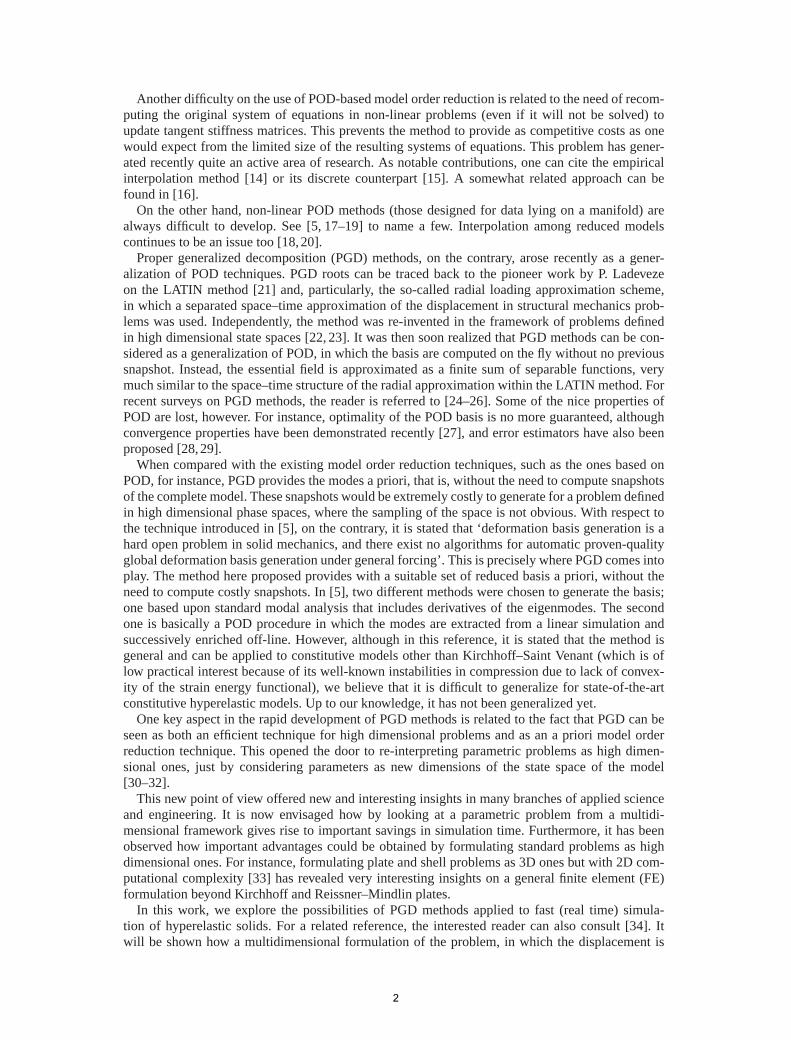
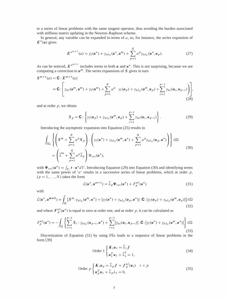
Figure 1. Load-displacement curve (in terms of the load parameter �) for one particular load position of thepinched cube problem. Different solutions for different orders of expansion (p D 1, : : : , 5) compared with

the FE solution by employing Newton–Raphson algorithms.

X

Y

Z

Uz

-0.01-0.02-0.03-0.04-0.05-0.06-0.07-0.08-0.09-0.1-0.11-0.12-0.13-0.14-0.15-0.16-0.17-0.18

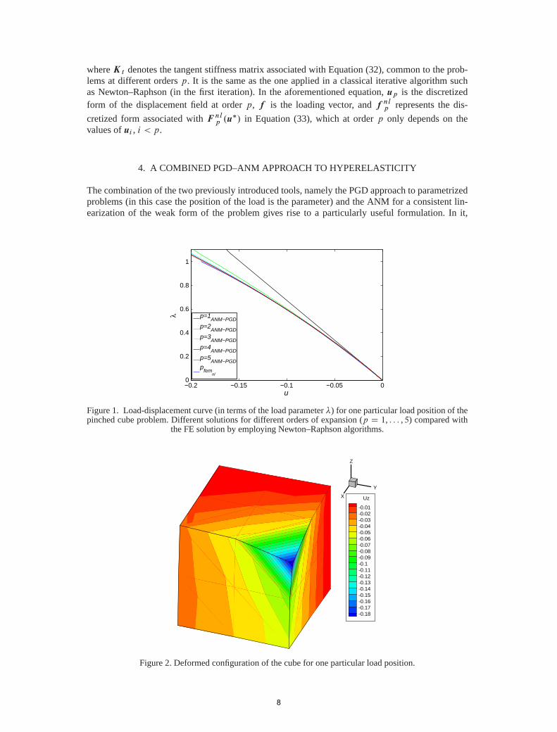
Figure 2. Deformed configuration of the cube for one particular load position.

8

the displacement field is approximated as a series expansion around the last equilibrium point,whereas each term of the series is considered to be approximated by a finite sum of separatedfunctions,

umC1 D umC a

n1XiD1

�F 1i ıG

1i

�C a2

n2XjD1

�F 2j ıG

2j

�C : : :C ap

npXlD1

�Fp

lıG

p

l

�. (36)

This gives rise to a series of problems of the form (34)–(35), within which a traditional PGD problemis solved for functions F ji .x/ and G j

i .s/ at each order of the expansion j . No further modificationof the method is necessary, resulting in a series of standard PGD problems that can be solved byemploying any of the available non-linear solvers. Here, as in many of our previous works, we haveemployed a fixed point algorithm, similar to the one sketched in Sections 2.1–2.2 before.

We study the behavior of the proposed technique by means of a series of benchmark problems inSection 5.

Y

X

Z

Uz

-20-40-60-80-100-120-140-160-180-200

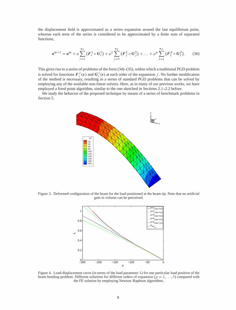
Figure 3. Deformed configuration of the beam for the load positioned at the beam tip. Note that no artificialgain in volume can be perceived.

−250 −200 −150 −100 −50 00

0.2

0.4

0.6

0.8

1

u

λ

p=1ANM−PGD

p=2ANM−PGD

p=3ANM−PGD

p=4ANM−PGD

p=5ANM−PGD

pfem

nl

Figure 4. Load-displacement curve (in terms of the load parameter �) for one particular load position of thebeam bending problem. Different solutions for different orders of expansion (p D 1, : : : , 5) compared with

the FE solution by employing Newton–Raphson algorithms.

9

5. NUMERICAL EXAMPLES

5.1. Kirchhoff–Saint Venant material

We will consider two sets of examples. The first one is composed by three different benchmarktests over Kirchhoff–Saint Venant materials. Despite its simplicity and well-known limitations,Kirchhoff–Saint Venant approaches are very useful in the field of real-time simulation, because theyprovide a good compromise between realism in the deformation and computational cost [5, 10].

5.1.1. Pinched cube. A unit cube modeled by 3 � 3 � 3 nodes and a tetrahedral mesh is con-sidered. Young’s modulus of 1 MPa and Poisson’s coefficient of 0.25 are assumed. The cube isloaded by a vertical force (0.01 N) acting at any point of the top face. Results obtained with thebefore presented PGD–ANM approach are compared with traditional FE approaches, solved bystandard Newton–Raphson linearization strategies. For one particular position of the load (one cor-ner), the load-displacement curve is shown in Figure 1, whereas its deformed configuration is shownin Figure 2.

In general, as was the case in previous references such as [18], expansions up to order six areenough to obtain a reasonable accuracy, despite the fact that in the ANM community, much higherorder expansions are usually employed on the order of 15 [38]. The number of modes (separated

X

Y

Z ZX

Y

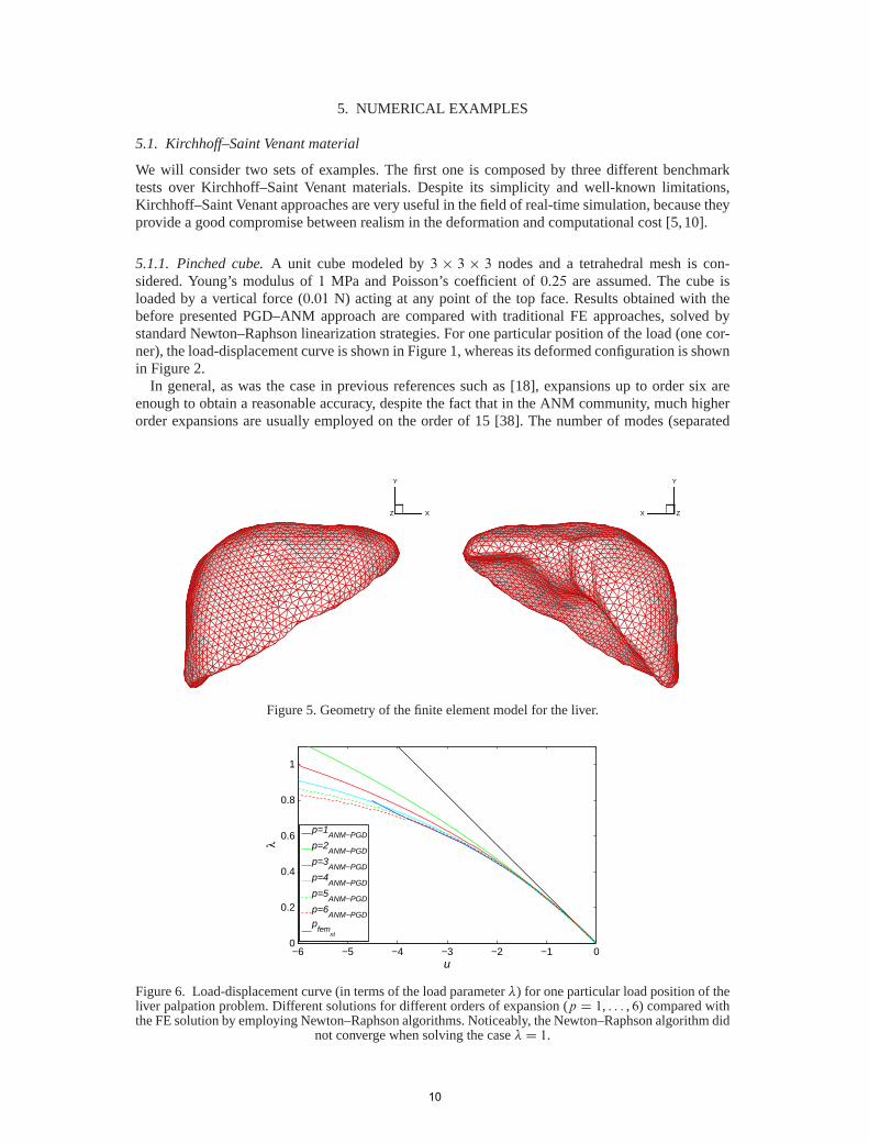
Figure 5. Geometry of the finite element model for the liver.

−6 −5 −4 −3 −2 −1 00

0.2

0.4

0.6

0.8

1

u

λ

p=1ANM−PGD

p=2ANM−PGD

p=3ANM−PGD

p=4ANM−PGD

p=5ANM−PGD

p=6ANM−PGD

pfem

nl

Figure 6. Load-displacement curve (in terms of the load parameter �) for one particular load position of theliver palpation problem. Different solutions for different orders of expansion (p D 1, : : : , 6) compared withthe FE solution by employing Newton–Raphson algorithms. Noticeably, the Newton–Raphson algorithm did

not converge when solving the case �D 1.

10

functions) employed at each expansion term in this example was 17, 17, 11, 2, 1 and 1, respectively,for terms of orders one to six. The accuracy of the approach is noteworthy, despite the fact thatterms 5 and 6 of the expansion (solution for the sixth order expansion is not depicted in Figure 1,because it is practically indistinguishable from that of order five) are obtained with only one coupleF .x/ ıG .s/, that is, n5 D n6 D 1 in Equation (36).

X

Y

Z

Uy

-0.1-0.2-0.3-0.4-0.5-0.6-0.7-0.8-0.9-1-1.1-1.2

Figure 7. Vertical displacement field of the Kirchhoff–Saint Venant liver for one particular position ofthe load.

X

Y

Z

Uy

0.0150.010.0050

-0.005-0.01-0.015-0.02-0.025-0.03-0.035-0.04-0.045-0.05-0.055-0.06-0.065

(a)

X

Y

Z

Uy

0.0150.010.0050

-0.005-0.01-0.015-0.02-0.025-0.03-0.035-0.04-0.045-0.05-0.055-0.06-0.065

(b)

X

Y

Z

Uy

0.0350.030.0250.020.0150.010.0050

-0.005-0.01-0.015-0.02-0.025-0.03

(c)

X

Y

Z

Uy

0.0220.020.0180.0160.0140.0120.010.0080.0060.0040.0020

-0.002-0.004-0.006-0.008-0.01-0.012

(d)

Figure 8. Functions F 1i .x/, for i D 1, 2, 3, and 20, respectively, for the first order expansion, in thesimulation of the Kirchhoff–Saint Venant liver.

11

5.1.2. Beam bending. In this case, we consider the problem of beam bending. This simple test isamong the most popular ones in the field of real-time simulation, because it readily shows a greatdivergence from physical results if a poor formulation is used [43]. In fact, if linear elasticity formu-lations are employed, a great gain of volume is observed, leading the observer to perceive a clearlynon-physical result, see Figure 3.

In this case, we consider a squared cross-section beam, with 40�40�400mm. Young’s moduluswas assumed to be 209, 000 MPa, whereas Poisson coefficient was set to 0.3. A load of 106 N canbe applied at any point of the upper face of the beam. Under these conditions, a comparison wasestablished between the tip displacement obtained for the load position at the beam rightmost sidewith the value obtained by using standard FE analysis and Newton–Raphson iterations to solve thenon-linear equations.

Results for different expansion order are shown in Figure 4. For a fifth order expansion, almostno difference can be perceived between the FE result and the reduced PGD–ANM result. For thisexample, the number of separated functions necessary at each expansion order was 162, 102, 79,161, 24, and 8, respectively. As stopping criterion, we employed a relative one, which stops thefixed point algorithm if the new functional pair contributes less than 10�4 times the initial pair offunctions, and a general one in which the algorithm is stopped if the modulus of the new functionalpair is less than 10�15.

In general, results are below 5% error with respect to the target FE solution of the problem. In anycase, a higher number of modes for each term, or a higher number of terms in the expansion, hasbeen shown to converge to the right solution. It is true, in general, that the number of off-line com-puted modes depends on the error estimator considered (see the works by Huerta [28] or Chamoin

X

Y

Z

Uy

3E-062E-061E-060

-1E-06-2E-06-3E-06-4E-06-5E-06-6E-06-7E-06-8E-06

(a)

X

Y

Z

Uy

2E-051.8E-051.6E-051.4E-051.2E-051E-058E-066E-064E-062E-060

(b)

X

Y

Z

Uy

2.5E-062E-061.5E-061E-065E-070

-5E-07-1E-06-1.5E-06-2E-06-2.5E-06-3E-06-3.5E-06-4E-06-4.5E-06-5E-06-5.5E-06

(c)

X

Y

Z

Uy

0

(d)

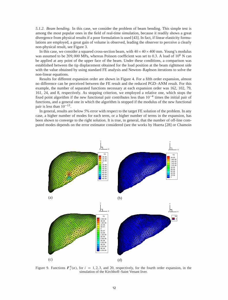
Figure 9. Functions F 4i .x/, for i D 1, 2, 3, and 20, respectively, for the fourth order expansion, in thesimulation of the Kirchhoff–Saint Venant liver.

12

and Ladeveze [29]). At present, there are no efficient and robust error estimators applicable to gen-eral multiparametric non-linear models. For this reason, we computed many terms (remember thatthis calculation is carried out off-line and only once) and then we compared the solution for someparticular choices of the parameters with the one obtained with FEs to check the convergence andsolution accuracy.

5.1.3. Palpation of the liver. One of the most typical examples in real-time applications is that ofliver palpation in a laparoscopic virtual surgery procedure. The liver is the biggest gland in thehuman body, after the skin. Liver geometry has been obtained from the SOFA project [43] andpost-processed to obtain a mesh composed by 2853 nodes and 10,519 tetrahedra, whose geometryis shown in Figure 5. The anterior surface of the liver is considered free, whereas the posterior onewas assumed to be supported over different organs (it is connected to the diaphragm by the coro-nary ligament, for instance). The inferior vena cava travels along the posterior surface, and the liveris frequently assumed clamped a that location. Although the assumed boundary conditions are notstrictly correct from a physiological point of view, our main interest is to show that the model canbe solved under real-time constraints with reasonable accuracy.

Here, the human liver is considered as a Kirchhoff–Saint Venant material with E D 0.17 MPaand � D 0.48 [44]. A vertical load of 5 N is considered at any point of the anterior surface of theliver. Again, for comparison purposes, results are evaluated at a particular position of the load andcompared with those obtained with a traditional FE analysis and standard Newton–Raphson iterativeschemes. It can be noticed how the sixth order expansion gives very reasonable results if comparedwith that of the FE model (Figure 6).

ZX

Y

F

43.532.521.510.50

(a)

ZX

Y

F

4.543.532.521.510.50

-0.5-1-1.5-2-2.5-3

(b)

ZX

Y

F

3.532.521.510.50

-0.5-1-1.5-2-2.5-3-3.5-4-4.5

(c)

ZX

Y

F

9876543210

-1-2-3-4-5-6-7-8

(d)

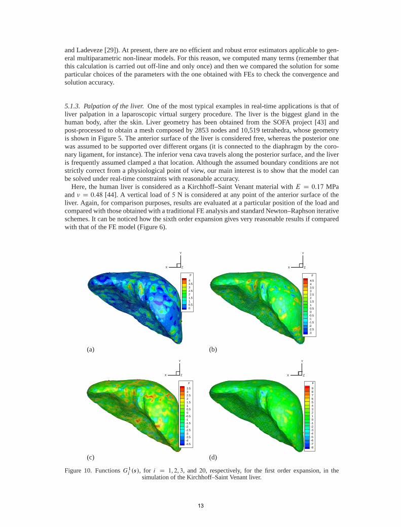
Figure 10. Functions G1i.s/, for i D 1, 2, 3, and 20, respectively, for the first order expansion, in the

simulation of the Kirchhoff–Saint Venant liver.

13

The vertical displacement field for that particular position of the load is depicted in Figure 7. Tocheck the overall behavior of the technique, functions F i and G i (Equation (36)) for i D 1, 2, 3,and 20 (terms of first and fourth order expansions) are shown in Figures 8–11.

5.2. Neo-Hookean behavior

Extension of the before presented technique to neo-Hookean materials [45] is in principle straight-forward, although lengthy (this is not important, in fact, because the parametric calculation iscarried out off-line). The major difference with the Kirchhoff–Saint Venant model is the presenceof material non-linearities, in addition to the geometrical ones. A POD–ANM approach has beensuggested in a previous work of the authors, see [18], and is here extended to the before presentedPGD framework.

The compressible neo-Hookean model is characterized by a strain energy function given by

‰ D�

2.tr.C /� 3/�� lnJ C

�

2.lnJ /2, (37)

where � and � are Lame’s constants and C D I C 2E is the right Cauchy-Green strain tensor. Thesecond Piola–Kirchhoff stress tensor can be obtained by

S D@‰.E/

@ED �.I �C�1/C �.lnJ /C�1. (38)

ZX

Y

F

160150140130120110100908070605040302010

(a)

ZX

Y

F

170160150140130120110100908070605040302010

(b)

ZX

Y

F

150140130120110100908070605040302010

(c)

ZX

Y

F

120110100908070605040302010

(d)

Figure 11. Functions G4i.s/, for i D 1, 2, 3, and 20, respectively, for the fourth order expansion, in the

simulation of the Kirchhoff–Saint Venant liver.

14

In this case, the intricate expansion procedure becomes easier if we identify, as in [37], the asymp-totic expansion with a Taylor series of the variables of interest, denoted by U .a/, in the vicinity ofaD 0. Truncating at order N .

U .a/D U 0C

NXpD1

U pap , (39)

where U 0 D U .0/ and

U p D1

pŠ

dpU

dap

�aD0

. (40)

XY

Z

Uz

-20-40-60-80-100-120-140-160-180-200-220-240-260-280

Order 1

Order 2

Order 3

Order 4

Figure 12. Solution for the neo-Hookean beam bending problem at different expansion orders.

−350 −300 −250 −200 −150 −100 −50 00

0.2

0.4

0.6

0.8

1

u

λ

p=1ANM−PGD

p=2ANM−PGD

p=3ANM−PGD

p=4ANM−PGD

pfem

nl

Figure 13. Solution for the neo-Hookean beam bending problem at different expansion orders.

15

In this case, as in [17], we have selected the following variables to perform the expansion,

U .a/D

0BBBBBBBB@

u.a/

S .a/

J 2C�1.a/

lnpJ 2.a/1J 2.a/

�.a/

1CCCCCCCCA

. (41)

By performing the substitution of the aforementioned variables into the weak form of the problem(Equation (21)), we arrive to a problem entirely similar to that in Equations (34) and (35). The entiredetails are provided, for completeness, in Appendix 1.

5.2.1. Neo-Hookean beam under bending. We reproduce here the problem in Section 5.1.2 butconsidering a neo-Hookean constitutive model. The deformed configuration of the beam at expan-sion orders one to four is depicted in Figure 12. Note how the first order expansion (linear approach)shows a tremendous gain in volume that renders the simulations clearly non-physical. Again, expan-sions up to orders four to six were judged sufficient to obtain a good approximation to the referencesolution (Figure 13). Obviously, higher accuracy can be obtained by increasing even more theexpansion order. Up to p D 15 is a typical value of the expansion order in the ANM literature.

5.2.2. Palpation of a neo-Hookean liver. The same procedure has been applied to the problem inSection 5.1.3 but now considering neo-Hookean behavior. The neo-Hookean law in Equation (37)has been now particularized toE D 0.17MPa and � D 0.48. As in previous examples, a PGD–ANMsolution has been obtained and compared with a standard FE solution at a particular node. To thisend, standard Newton–Raphson procedures have been employed for the solution of the resultingnon-linear system of equations. The load-displacement curve for this particular node is shown inFigure 14.

In this case, the observed agreement between the PGD–ANM solution and that of the FE modelis even higher than in the previous example. For the fourth order expansion, the agreement betweenthe predicted load-displacement curves is almost exact.

Remember that our approach is based upon an off-line/online procedure such that, once the off-line computation has been carried out, its solution is stored in the form of a series of 1D vectors thatare evaluated in real time very efficiently. The solution thus computed is a multidimensional one,that is particularized online. This procedure is sketched in Figure 15.

−6 −5 −4 −3 −2 −1 00

0.2

0.4

0.6

0.8

1

uy

λ

p=1ANM−PGD

p=2ANM−PGD

p=3ANM−PGD

p=4ANM−PGD

pfem

nl

Figure 14. Comparison between the PGD–ANM solution, at different expansion orders, and that for astandard finite element solution for a load at a particularized position. Neo-Hookean behavior.

16

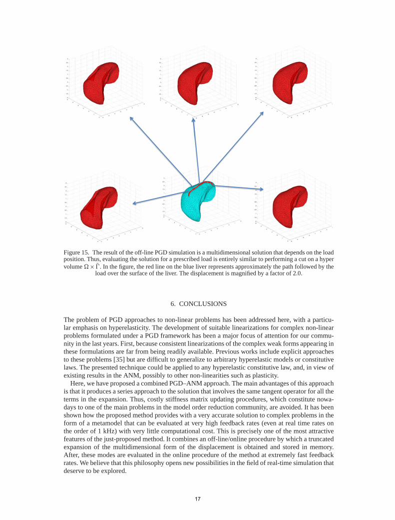
Figure 15. The result of the off-line PGD simulation is a multidimensional solution that depends on the loadposition. Thus, evaluating the solution for a prescribed load is entirely similar to performing a cut on a hypervolume �� N� . In the figure, the red line on the blue liver represents approximately the path followed by the

load over the surface of the liver. The displacement is magnified by a factor of 2.0.

6. CONCLUSIONS

The problem of PGD approaches to non-linear problems has been addressed here, with a particu-lar emphasis on hyperelasticity. The development of suitable linearizations for complex non-linearproblems formulated under a PGD framework has been a major focus of attention for our commu-nity in the last years. First, because consistent linearizations of the complex weak forms appearing inthese formulations are far from being readily available. Previous works include explicit approachesto these problems [35] but are difficult to generalize to arbitrary hyperelastic models or constitutivelaws. The presented technique could be applied to any hyperelastic constitutive law, and, in view ofexisting results in the ANM, possibly to other non-linearities such as plasticity.

Here, we have proposed a combined PGD–ANM approach. The main advantages of this approachis that it produces a series approach to the solution that involves the same tangent operator for all theterms in the expansion. Thus, costly stiffness matrix updating procedures, which constitute nowa-days to one of the main problems in the model order reduction community, are avoided. It has beenshown how the proposed method provides with a very accurate solution to complex problems in theform of a metamodel that can be evaluated at very high feedback rates (even at real time rates onthe order of 1 kHz) with very little computational cost. This is precisely one of the most attractivefeatures of the just-proposed method. It combines an off-line/online procedure by which a truncatedexpansion of the multidimensional form of the displacement is obtained and stored in memory.After, these modes are evaluated in the online procedure of the method at extremely fast feedbackrates. We believe that this philosophy opens new possibilities in the field of real-time simulation thatdeserve to be explored.

17

Other problems remain open, however. Notably, optimality of PGD approaches (i.e., under whatcircumstances a priori PGD modes are equivalent to a posteriori POD or SVD modes) is not wellunderstood. It has been noticed in the examples throughout this work that, unlike those in previousexplicit approaches, PGD–ANM modes seem not to be optimal. They are highly oscillating andnumerous for a prescribed tolerance. The solution is simple, however. It suffices to obtain the SVDmodes that show most of the energy of the system to obtain a very compact representation of thesolution (the so-called projected PGD, see [46]). But in any case, it seems pertinent to work in dis-cerning what are the key ingredients of optimality in a PGD approach. This constitutes one of ourcurrent efforts of research.

In any case, although not optimal, the proposed method provides with a very competitive solu-tion to highly demanding problems in applied sciences and engineering such as dynamic data-driven problems, real-time response even under very restrictive scenarios (haptic peripherals, forinstance), simulation-driven control of structures and processes, and many others, where non-linearsimulations are nowadays standard in industrial practice.

APPENDIX A: DERIVATION OF THE TANGENT STIFFNESS MATRIX FOR THENEO-HOOKEAN CASE

For the neo-Hookean case explained in Section 5.2, the tangent stiffness matrix takes the followingform:

K t D

Z�0

�BTDB CGT QS 0G

�d�, (A.1)

where

D D �

�1

J 20C�10 M

T0

�C 2.�� � lnJ0/

�1

J 20

�C�10 M

T0

�� QC 0

�(A.2)

now takes into account the material non-linearity and has a somewhat similar appearance tothe Lagrangian elastic tensor at the initial state. J0 and C 0 represent the Jacobian and rightCauchy-Green strain tensor of the initial solution. M0 is obtained from the series expansion ofthe Jacobian, and contains minors of C 0. Finally, QC 0 is obtained from the series expansion of C�1

and contains components of C 0, arranged in a particular way.The geometrical non-linearities are included in the matricesB,G , and QS 0.B represents the usual

strain-displacement matrix, G relates the nodal displacements u and the gradient of displacementsvector, and, finally, QS 0 represents a matrix that contains the initial stresses (we have chosen thesame notation as in [39]).

In the right-hand side of Equation (35), the non linear load vector f nlp is a vector containinginformation of material and geometrical non-linearities of all order problems ranging from orderone to p � 1. It can be written as

f nlp D

Z�0

�BT

�S nlmatp C S nlgeom

p

�CGTS �p

�d� (A.3)

As in the stiffness matrix, S nlgeomp and S �p represent the standard matrices found in literature

when ANM is used to solve geometrical non-linear problems with linear materials. S nlmatp takes

into account the material behavior,

S nlmatp D .� lnJ0 ��/

�CC 0

�RZp �

RJp

J 40

�CRCC p

J 20CRC�1p

�

C �

�CC 0

J 20

�RYp C

RJp

2J 20

�CRSp

�. (A.4)

18

In this equation, CC 0 represents the cofactor matrix of C 0, and RCC p is a vector containingvalues of Cij of all problems from order one to p � 1, obtained when the cofactor matrix of C isexpanded in Taylor series,

CC p D QC 0C p CRCC p , (A.5)

RCC p D

p�1XrD1

0BBBBBBBBBB@

C r22Cp�r33 �C r23C

p�r23

C r11Cp�r33 �C r13C

p�r13

C r11Cp�r22 �C r12C

p�r12

C r13Cp�r23 �C r12C

p�r33

C r13Cp�r12 �C r11C

p�r23

C r12Cp�r23 �C r13C

p�r22

1CCCCCCCCCCA

. (A.6)

Here, RJp is a summation of products of different components of C p and is obtained when thesquared Jacobian is expanded in Taylor series,

.J 2/p DMT0 C p CRJp . (A.7)

RSp collects terms concerning the expansion of Y D lnJ and C�1,

RSp D

p�1XrD1

YrC�1p�r . (A.8)

RC�1p collects terms concerning Z D J�2 and cofactor matrix of C expansions,

RC�1p D

p�1XrD1

ZrCC p�r . (A.9)

Finally, it is necessary to expand Y D lnJ and Z D J�2 by using Taylor series and the chainrule generalized to higher derivatives,

Yp D1

2J 20.J 2/p CRYp , and Zp D

�1

J 40.J 2/p CRZp , (A.10)

where

RY1 D 0,

RY2 D�1

4J 40.J 2/21

�,

RY3 D1

6J 60.J 2/31C 2

�1

4J 40.J 2/1.J

2/2,

RZ1 D 0,

RZ2 D1

J 60.J 2/21,

RZ3 D�1

J 80.J 2/31C 2

1

J 60.J 2/1.J

2/2,

: : :

At this point, a procedure entirely similar to that of Equation (36) is performed, leading to anequivalent expression of the displacement in terms of a power series in parameter a, where eachterm is composed by a finite sum of separable functions.

19

ACKNOWLEDGEMENT

The authors would wish to thank the Spanish Ministry of Economy and Innovation (grant number,CICYT-DPI2011-27778-C02-01) for their support.

REFERENCES

1. Karhunen K. Über lineare methoden in der wahrscheinlichkeitsrechnung. Annales Academiae Scientiarum FennicaeSeries A1 Mathematical Physics 1946; 37:1–79.

2. Loève MM. Probability Theory, 3rd ed., The University Series in Higher Mathematics. Van Nostrand: Princeton, NJ,1963.

3. Lorenz EN. Empirical Orthogonal Functions and Statistical Weather Prediction. Scientific Report Number 1,Statistical Forecasting Project, MIT, Departement of Meteorology, 1956.

4. Park HM, Cho DH. The use of the Karhunen–Loève decomposition for the modeling of distributed parametersystems. Chemical Engineering Science 1996; 51(1):81–98.

5. Barbic J, James DL. Real-time subspace integration for St. Venant–Kirchhoff deformable models. ACM Transactionson Graphics (SIGGRAPH 2005) 2005; 24(3):982–990.

6. Idelsohn SR, Cardona R. A reduction method for nonlinear structural dynamics analysis. Computer Methods inApplied Mechanics and Engineering 1985; 49:253–279.

7. Krysl P, Lall S, Marsden JE. Dimensional model reduction in non-linear finite element dynamics of solids andstructures. International Journal for Numerical Methods in Engineering 2001; 51:479–504.

8. Niroomandi S, Alfaro I, Cueto E, Chinesta F. Real-time deformable models of non-linear tissues by model reductiontechniques. Computer Methods and Programs in Biomedicine 2008; 91(3):223–231.

9. Taylor ZA, Crozier S, Ourselin S. A reduced order explicit dynamic finite element algorithm for surgical simulation.IEEE Transactions on Medical Imaging 2011; 30(9):1713–1721.

10. Taylor ZA, Ourselin S, Crozier S. A reduced order finite element algorithm for surgical simulation. In Engineer-ing in Medicine and Biology Society (EMBC), 2010 Annual International Conference of the IEEE, Buenos Aires,Argentina, September 4–31, 2010; 239–242.

11. Ryckelynck D. A priori model reduction method for the optimization of complex problems. In Workshop on OptimalDesign of Materials and Structures, Ecole Polytechnique, Palaiseau, Paris (France), 2003.

12. Ryckelynck D. A priori hyperreduction method: an adaptive approach. Journal of Computational Physics 2005;202(1):346–366.

13. Ryckelynck D, Chinesta F, Cueto E, Ammar A. On the a priori model reduction: overview and recent developments.Archives of Computational Methods in Engineering 2006; 12(1):91–128.

14. Barrault M, Maday Y, Nguyen NC, Patera AT. An ‘empirical interpolation’ method: application to efficientreduced-basis discretization of partial differential equations. Comptes Rendus Mathematique 2004; 339(9):667–672.

15. Chaturantabut S, Sorensen DC. Nonlinear model reduction via discrete empirical interpolation. SIAM Journal ofScientific Computing 2010; 32:2737–2764.

16. Nguyen NC, Patera AT, Peraire J. A ‘best points’ interpolation method for efficient approximation of parametrizedfunctions. International Journal for Numerical Methods in Engineering 2008; 73(4):521–543.

17. Niroomandi S, Alfaro I, Cueto E, Chinesta F. Accounting for large deformations in real-time simulations of softtissues based on reduced-order models. Computer Methods and Programs in Biomedicine 2012; 105(1):1–12.

18. Niroomandi S, Alfaro I, Cueto E, Chinesta F. Model order reduction for hyperelastic materials. International Journalfor Numerical Methods in Engineering 2010; 81(9):1180–1206.

19. Tenenbaum JB, de Silva V, Langford JC. A global framework for nonlinear dimensionality reduction. Science 2000;290:2319–2323.

20. Amsallem D, Farhat Ch. An interpolation method for adapting reduced-order models and application to aeroelasticity.AIAA Journal 2008; 46:1803–1813.

21. Ladeveze P. Nonlinear Computational Structural Mechanics. Springer: N.Y., 1999.22. Ammar A, Mokdad B, Chinesta F, Keunings R. A new family of solvers for some classes of multidimensional partial

differential equations encountered in kinetic theory modeling of complex fluids. Part II: transient simulation usingspace-time separated representations. Journal of Non-Newtonian Fluid Mechanics 2007; 144:98–121.

23. Ammar A, Mokdad B, Chinesta F, Keunings R. A new family of solvers for some classes of multidimensional partialdifferential equations encountered in kinetic theory modeling of complex fluids. Journal of Non-Newtonian FluidMechanics 2006; 139:153–176.

24. Chinesta F, Ammar A, Cueto E. Recent advances in the use of the proper generalized decomposition for solvingmultidimensional models. Archives of Computational Methods in Engineering 2010; 17(4):327–350.

25. Chinesta F, Ladeveze P, Cueto E. A short review on model order reduction based on proper generalizeddecomposition. Archives of Computational Methods in Engineering 2011; 18:395–404.

26. Ladeveze P, Passieux J-C, Neron D. The Latin multiscale computational method and the proper generalizeddecomposition. Computer Methods in Applied Mechanics and Engineering 2010; 199(21-22):1287–1296.

27. Le Bris C, Lelièvre T, Maday Y. Results and questions on a nonlinear approximation approach for solving high-dimensional partial differential equations. Constructive Approximation 2009; 30:621–651. 10.1007/s00365-009-9071-1.

20

28. Ammar A, Chinesta F, Diez P, Huerta A. An error estimator for separated representations of highly multidimensionalmodels. Computer Methods in Applied Mechanics and Engineering 2010; 199(25-28):1872–1880.

29. Ladeveze P, Chamoin L. On the verification of model reduction methods based on the proper generalizeddecomposition. Computer Methods in Applied Mechanics and Engineering 2011; 200(23-24):2032–2047.

30. Ghnatios Ch, Chinesta F, Cueto E, Leygue A, Poitou A, Breitkopf P, Villon P. Methodological approach to efficientmodeling and optimization of thermal processes taking place in a die: application to pultrusion. Composites Part A:Applied Science and Manufacturing 2011; 42(9):1169–1178.

31. Ghnatios Ch, Masson F, Huerta A, Leygue A, Cueto E, Chinesta F. Proper generalized decomposition-baseddynamic data-driven control of thermal processes. Computer Methods in Applied Mechanics and Engineering 2012;213-216(0):29–41.

32. Pruliere E, Chinesta F, Ammar A. On the deterministic solution of multidimensional parametric models using theProper generalized decomposition. Mathematics and Computers in Simulation 2010; 81(4):791–810.

33. Bognet B, Bordeu F, Chinesta F, Leygue A, Poitou A. Advanced simulation of models defined in plate geometries:3D solutions with 2D computational complexity. Computer Methods in Applied Mechanics and Engineering 2012;201-204(0):1–12.

34. Relun N, Neron D, Boucard P-A. A model reduction technique based on the PGD for elastic-viscoplasticcomputational analysis. Computational Mechanics 2013; 51:83–92.

35. Niroomandi S, Gonzalez D, Alfaro I, Bordeu F, Leygue A, Cueto E, Chinesta F. Real time simulation of biolog-ical soft tissues: a PGD approach. International Journal for Numerical Methods in Biomedical Engineering 2013;29(5):586–600.

36. Abichou H, Zahrouni H, Potier-Ferry M. Asymptotic numerical method for problems coupling several nonlinearities.Computer Methods in Applied Mechanics and Engineering 2002; 191(51-52):5795–5810.

37. Cao H-L, Potier-Ferry M. An improved iterative method for large strain viscoplastic problems. International Journalfor Numerical Methods in Engineering 1999; 44:155–176.

38. Cochelin B, Damil N, Potier-Ferry M. Asymptotic-numerical methods and Padé approximants for non-linear elasticstructures. International Journal for Numerical Methods in Engineering 1994; 37:1187–1213.

39. Cochelin B, Damil N, Potier-Ferry M. The asymptotic numerical method: an efficient perturbation technique fornonlinear structural mechanics. Revue Europeenne des Elements Finis 1994; 3:281–297.

40. Gonzalez D, Masson F, Poulhaon F, Cueto E, Chinesta F. Proper generalized decomposition based dynamic datadriven inverse identification. Mathematics and Computers in Simulation 2012; 82:1677–1695.

41. Bro-Nielsen M, Cotin S. Real-time volumetric deformable models for surgery simulation using finite elements andcondensation. Computer Graphics Forum 1996; 15(3):57–66.

42. Yvonnet J, Zahrouni H, Potier-Ferry M. A model reduction method for the post-buckling analysis of cellularmicrostructures. Computer Methods in Applied Mechanics and Engineering 2007; 197:265–280.

43. Allard J, Cotin S, Faure F, Bensoussan P-J, Poyer F, Duriez C, Delingette H, Grisoni L. SOFA – an open sourceframework for medical simulation. In Medicine Meets Virtual Reality (MMVR’15), Long Beach, USA, February2007; 13–18.

44. Delingette H, Ayache N. Soft tissue modeling for surgery simulation. In Computational Models for the Human Body,Ayache N (ed.), Handbook of Numerical Analysis (Ph. Ciarlet, Ed.) Elsevier: Juan-les-Pins, France, 2004; 453–550.

45. Bonet J, Wood RD. Nonlinear Continuum Mechanics for Finite Element Analysis. Cambridge University Press: NewYork, 2008.

46. Nouy A. A priori model reduction through proper generalized decomposition for solving time-dependent partialdifferential equations. Computer Methods in Applied Mechanics and Engineering 2010; 199(23-24):1603–1626.

21