Model Order Reduction using SPICE Simulation Traces

Paul Winkler, Henda Aridhi, and Sofiene Tahar

Department of Electrical and Computer Engineering,Concordia University, Montreal, Canada

pauwink@web.de, h aridh@ece.concordia.ca, tahar@ece.concordia.ca

Technical Report

December 1, 2013

Abstract

The generation of fast models for device level circuit descriptions is a very active area of research. Model

order reduction is an attractive technique for reducing the computational cost of dynamical models

simulation. In this work, we propose an approach based on clustering, curve-fitting, linearization and

Krylov space projection to build reduced models for nonlinear analog circuits. We demonstrate our

model order reduction method for three nonlinear circuits: a voltage controlled oscillator, an operational

amplifier and a digital frequency divider. Our experimental results show that the reduced models lead

to an improvement in simulation speed while providing the same behavior of the original circuit design.

1

1 Introduction

Large electronic circuits are very complicated systems. Due to their usual large size andstrong nonlinear characteristics, the only way to analyse them is a computer simulation.Simulation programs with integrated circuit emphasis (SPICE) are used widely to analyseor design electronic circuits. The elements of these circuits are usually integrated on a singlesemiconductor layer of an integrated circuit (IC) or as single devices on a printed circuitboard (PCB). The continuously improving technology enables the production of smaller andsmaller devices and their implementation on a single IC. Following the Moores law, thenumber of elements per IC grows exponentially and can reach today 109 and more. Thistrend is predicted to continue in the next decades [1]. Also the numerical solvers, which areused to compute the behaviour of circuits, e.g., in SPICE programs, are very advanced, thehigh number of elements in a large circuit forces the simulation to slow down. This increasesdevelopment time and costs for the design of new circuits.

Model order reduction (MOR) techniques, which are able to reduce the size of a dynam-ical system description, were recently applied to find smaller and faster models of electroniccircuits [2, 3]. The most promising MOR approaches for nonlinear circuits use the timetraces, resulting from a circuit transient simulation, to find linearization points of an alreadyelaborated mathematical model of the circuit [4, 5, 6]. This report investigates, whetherthe time traces of a former transient simulation of an electronic circuit can be used to findthe mathematical description of the circuit, by using curve-fitting. The elaborated mathe-matical model can be used, if the parameters of the original system are partially unknownor the device models are to complex to elaborate their mathematical model analytically.The new model, which is elaborated by curve-fitting, is a simplified approximation of theoriginal circuit model in its original state space. It will contain less details than the originaldescription of the circuit, which is enclosed in a SPICE netlist. For the reduction of thesystem, a Krylov algorithm is used. The simulation of the generated, reduced models shouldbe faster than the simulation of the original models. Also this models are a modification,it is essentially, that they accurately show the behaviour of the original model. It has tobe explored, whether the generation of reduced analog circuit models can be automated, byusing their time traces, and whether these models are an alternative to conventional circuitmodels.

Section 3 explains briefly the main techniques to model an electronic circuit mathemati-cally and to compute the time traces of its signals. It also introduces the basics of MOR andexplains the projection based MOR technique of nonlinear ODE-systems, which is equal tothe methods discussed in [4, 5]. Section 4 shows, how to use simulation time traces to findthe mathematical description of linear and nonlinear circuits. The challenges of curve-fittingthe simulation results and required additional information to find a proper mathematicalmodel are discussed. Different curve-fitting methods for the curve-fitting are shown. Thetechniques introduced in Section 3 and 4 are connected together to the final model generationmethodology, which is presented in Section 5. In this Section the requirements of a reducedmodel are discussed. The usefulness of the model generation approach is demonstrated onthree applications in Section 6.

The work is concluded and aspects of future work are given in Section 7.

2 Related Work

In the last two decades many researchers realized the possibilities offered by MOR for dy-namic systems and tried to improve and apply these methods in practice [2, 3].

2

Many approaches for linear circuits work on the approximation of the transfer function.Truncation methods as shown in [7] and [8] cut and simplify the transfer function of linearcircuits, ensuring the difference between the original and reduced transfer function to stayin a specified range. Therefore the transfer function is developed in polynomial form, usingpade approximation [9] or similar techniques, and cut after the most significant terms.

Proper Orthogonal Decomposition (POD) is a method which replaces a correlation ma-trix, characterizing the system, by a smaller matrix, holding the the same significant eigen-values [10]. POD can be interpreted as a mean to compute a Krylov subspace. Other waysto find a smaller subspace are iterative methods like Arnoldi and Lanczos algorithm, whichare discussed as MOR techniques, e.g., in [4, 5, 11, 12]. These iterative techniques have theadvantage of a low computation effort. Working on the reduction of square matrices, theycompute the significant eigenvalues and eigenvectors. This most significant vectors build aprojection matrix to transform the model to a subspace.

All of these methods work fine for linear systems [3, 7, 8]. They can, for example, describelarge RLC-networks, which occur especially in models of wire interconnection in every elec-tronic network. To apply MOR techniques to nonlinear systems, they have to be modified.

A simple approach, which can be used for circuits with only a few nonlinear elements, isintroduced in [13]. Dividing a circuit in linear and nonlinear subcircuits, the mathematicalmodel of the linear part of the circuit is decoupled from the nonlinear part, reduced andagain linked to the nonlinear part.

A technique to include the nonlinear part into the reduction is the trajectory piecewiseMOR introduced in [4, 5]. This approaches transforms the strong nonlinear system to apiecewise linear system and applies a Krylov algorithm on them. A similar technique, whichis introdued in [6], uses piecewise polynomial instead of piecewise linear systems, to replacethe nonlinear system. Also for this approach Krylov methods are used, as the reductionworks on square matrices of the system state space description. All approaches for the re-duction of a nonlinear system need a first simulation of the original dynamic system witha training input. This simulation is used to explore the system state space and find properpoints for the development of a piecewise system.

System Modelling using Curve-Fitting

Curve-fitting techniques are used in many different scientific disciplines. Mostly experi-mental data is used to determine some parameters of well known functions, which describethe underlying physical process, e.g., the type and portion of a radio active element in anobject can be found by curve-fitting the function of the decay per time.

Also in the field of electrical engineering, curve-fitting is used. A general approachto describe the I-V-characteristic of semiconductor devices is to measure this curves in alaboratory experiment and use this curves to find typical parameters of the devices. Thistop-down modelling is very efficient and simple, as it uses the physical behaviour of a de-vice to describe it, instead of calculating its parameters from material and geometrical values[14]. Also SPICE programs themselves offer the possibility to calculate device parameters bycurve-fitting a set of data [15]. Nevertheless, in all these approaches curve-fitting is used todescribe the behaviour of a single device, using a set of data, which may includes around fouror five different physical quantities [14]. In this work we investigate to find the mathematicalmodel of a whole circuit, by curve-fitting a high number of different signals.

3

3 Preliminaries

3.1 Mathematical Modelling and Numerical Simulation

In many disciplines simulation is accepted as the third pillar of science, beside theory andexperiment [16]. Especially in the analysis and design of analog electronic circuits simulationit is a required method. It is the most exact and often the only possible way to analysethe dynamical system, which results from the connection of thousands and more nonlineardevices.

SPICE programs, which are the state of the art for analog circuit computation, havetwo main functionalities. At first they find a mathematical description of a circuit, which isdescribed by a netlist. Therefore, they use very detailed device models and the technique ofModified Nodal Analysis (MNA) [17]. For the transient analysis, the mathematical modelcan be a pure algebraic equation system (for a pure resistive circuit), a linear ODE or DAEsystem (circuit just consisting of linear resistances R, capacitances C and inductances L) or anonlinear ODE or DAE system (circuit includes active devices or nonlinear R, C or L). Thesecond functionality is to solve the generated equation system numerically. Therefore SPICEuses modified Trapezoidal or Backward Euler Algorithm [17, 18], which are introduced inSection 3.1.3.

In Section 3.1.1 is shown, how the three most common active devices, diode, bipolarjunction transistor (BJT) and field-effect transistor (FET), are replaced by their equivalentcircuit for a transient analysis. In Section 3.1.2 the theory and a practical example of theMNA are explained. The knowledge of this techniques are the basis for the curve-fitting ofthe time traces. They are required to select the signals, which are the state space variablesof the system, and are especially important to generate a function guess for the curve-fittingof the nonlinear systems, described in Chapter 4.

3.1.1 Equivalent Circuits

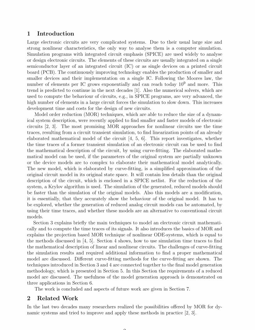
To prepare the circuit for the MNA, all active devices have to be replaced by their transientequivalent circuit. This will transform the electronic circuit to a network, which is completelydrawn by two-port elements. After the replacement, the circuit will just consist of theelements shown in Figure 1.

Fig. 1: Two-port Elements for Complete Circuit Modeling at the Device Level

Where the symbols show a capacitance (C), a resistance (R), an inductance (L), an in-dependent voltage source (V), an independent current source (I) and a voltage controlledcurrent source (G). In the following the transient equivalent circuits of the three most com-mon active devices of diode, BJT and FET are shown. The capacitances in the equivalentcircuits are junction or diffusion capacitances, depending on the state of the pn-junction.Resistances model the parasitic effect of nonideal conductors.

Diode

4

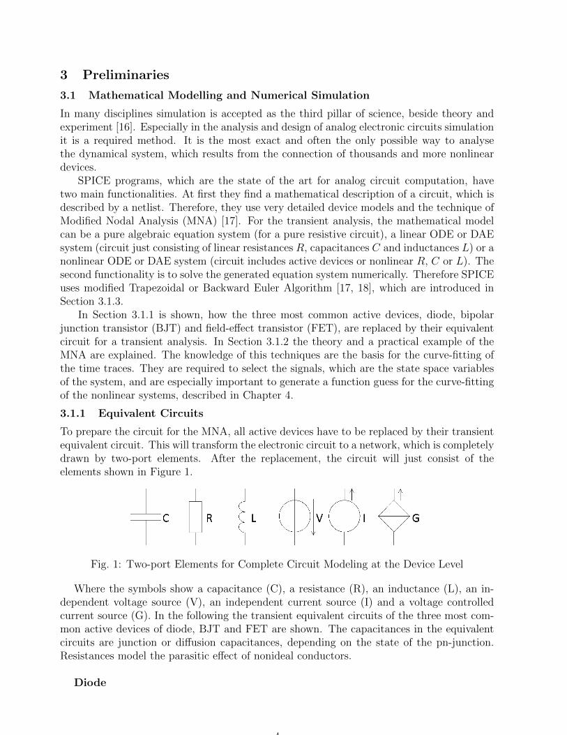
The diode semiconductor structure and its transient equivalent circuit are shown in Figure2, where Rs is the series resistance, Cd the junction capacitance and Gd a VCCS, whichfollows the I-V-characteristic of the pn-junction shown in Equation (1).

Fig. 2: Diode - Semiconductor Structure, Symbol and Transient Equivalent Circuit

Id = Is ·(e

VDn·VT

)(1)

Bipolar Junction Transistor

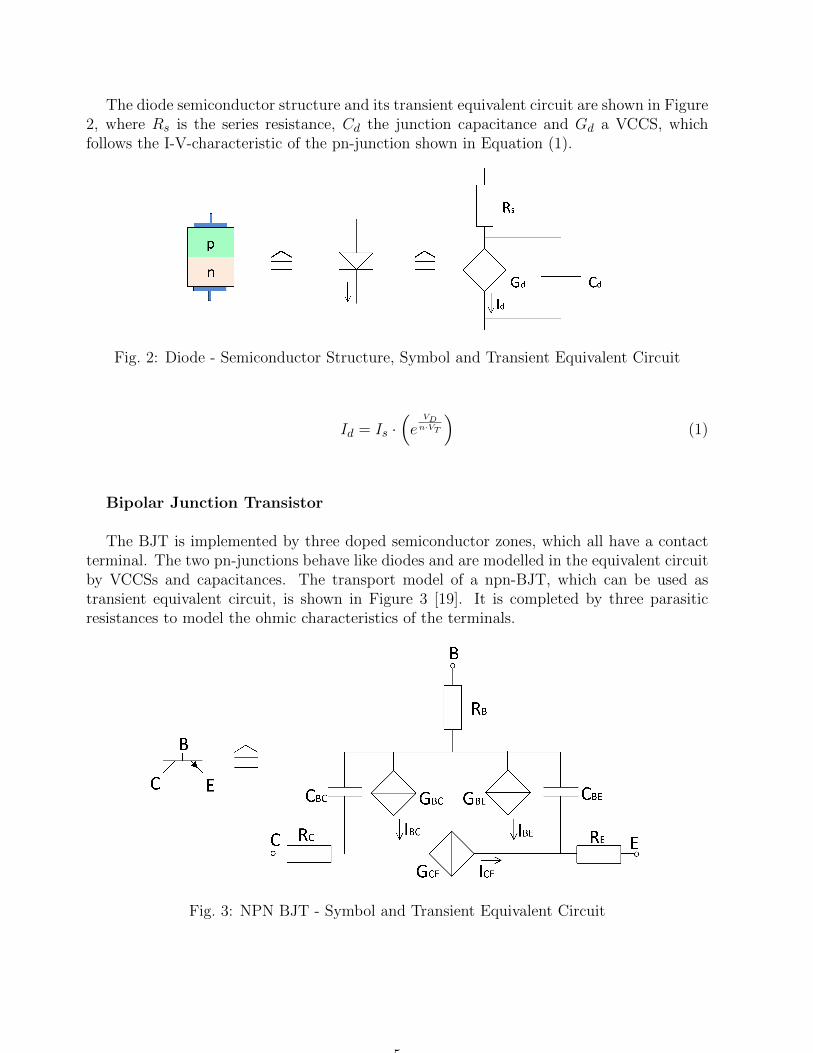
The BJT is implemented by three doped semiconductor zones, which all have a contactterminal. The two pn-junctions behave like diodes and are modelled in the equivalent circuitby VCCSs and capacitances. The transport model of a npn-BJT, which can be used astransient equivalent circuit, is shown in Figure 3 [19]. It is completed by three parasiticresistances to model the ohmic characteristics of the terminals.

Fig. 3: NPN BJT - Symbol and Transient Equivalent Circuit

5

The functions of the VCCSs of the equivalent circuit are the shown in the following.

IBC =IsBR· e

VBCVT

IBE =IsBN· e

VBEVT

ICE = Is ·(e

VBEVT − e

VBCVT

) (2)

Because of the very small gap between the two pn-junctions, they influence each otherand the base-current can control the collector current. The current IBC is close to zero forforward operation. For a pnp-transistor the current direction and the controlling voltages inthe VCCS functions are inverted.

Field-Effect Transistor

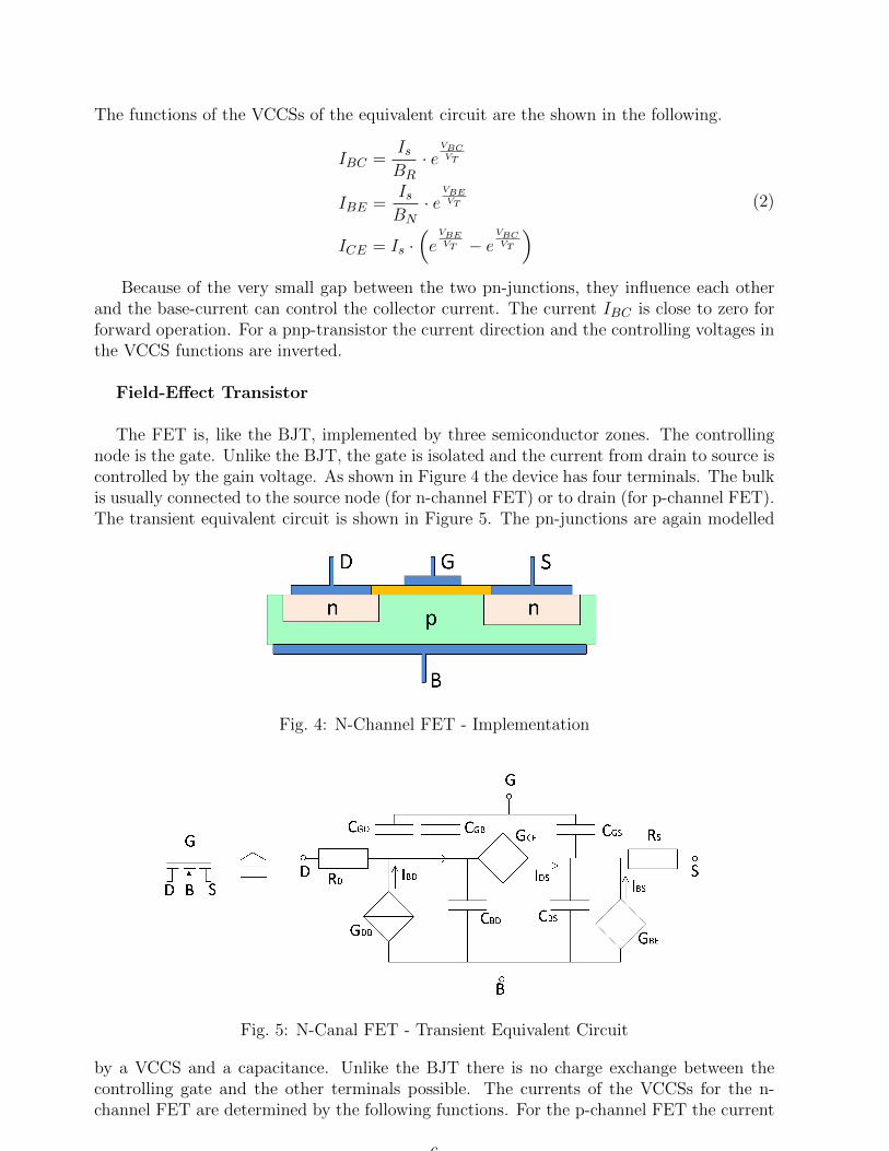
The FET is, like the BJT, implemented by three semiconductor zones. The controllingnode is the gate. Unlike the BJT, the gate is isolated and the current from drain to source iscontrolled by the gain voltage. As shown in Figure 4 the device has four terminals. The bulkis usually connected to the source node (for n-channel FET) or to drain (for p-channel FET).The transient equivalent circuit is shown in Figure 5. The pn-junctions are again modelled

Fig. 4: N-Channel FET - Implementation

Fig. 5: N-Canal FET - Transient Equivalent Circuit

by a VCCS and a capacitance. Unlike the BJT there is no charge exchange between thecontrolling gate and the other terminals possible. The currents of the VCCSs for the n-channel FET are determined by the following functions. For the p-channel FET the current

6

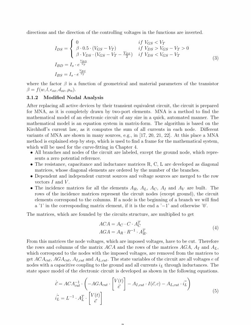
directions and the direction of the controlling voltages in the functions are inverted.

IDS =

0 if VGS < VTβ · 0.5 · (VGS − VT ) if VDS > VGS − VT > 0

β · VDS · (VGS − VT − VDS

2 ) if VDS < VGS − VT

IBD = Is · eVBDVT

IBS = Is · eVBSVT

(3)

where the factor β is a function of geometrical and material parameters of the transistorβ = f(w, l, εox, dox, µn).

3.1.2 Modified Nodal Analysis

After replacing all active devices by their transient equivalent circuit, the circuit is preparedfor MNA, as it is completely drawn by two-port elements. MNA is a method to find themathematical model of an electronic circuit of any size in a quick, automated manner. Themathematical model is an equation system in matrix-form. The algorithm is based on theKirchhoff’s current law, as it computes the sum of all currents in each node. Differentvariants of MNA are shown in many sources, e.g., in [17, 20, 21, 22]. At this place a MNAmethod is explained step by step, which is used to find a frame for the mathematical system,which will be used for the curve-fitting in Chapter 4.• All branches and nodes of the circuit are labeled, except the ground node, which repre-

sents a zero potential reference.• The resistance, capacitance and inductance matrices R, C, L are developed as diagonal

matrices, whose diagonal elements are ordered by the number of the branches.• Dependent and independent current sources and voltage sources are merged to the row

vectors I and V .• The incidence matrices for all the elements AR, AL, AC , AI and AV are built. The

rows of the incidence matrices represent the circuit nodes (except ground), the circuitelements correspond to the columns. If a node is the beginning of a branch we will finda ’1’ in the corresponding matrix element, if it is the end a ’−1’ and otherwise ’0’.

The matrices, which are founded by the circuits structure, are multiplied to get

ACA = AC · C · ATC

AGA = AR ·R−1 · ATR.

(4)

From this matrices the node voltages, which are imposed voltages, have to be cut. Thereforethe rows and columns of the matrix ACA and the rows of the matrices AGA, AI and AL,which correspond to the nodes with the imposed voltages, are removed from the matrices toget ACAcut, AGAcut, AI,cut and AL,cut. The state variables of the circuit are all voltages e ofnodes with a capacitive coupling to the ground and all currents iL through inductances. Thestate space model of the electronic circuit is developed as shown in the following equations.

~e = ACA−1cut ·

(−AGAcut ·

[V (t)~e

]− AI,cut · I(~e, c)− AL,cut · ~iL

)~iL = L−1 · AT

L ·[V (t)~e

] (5)

7

ODE-System Modelling Using Parasitic Elements

The shown MNA method will result in an ODE or DAE-system, depending on the circuititself. To ensure the resulting system to be easily manageable with numerical methods, thesystem should be an ODE-system. A DAE system is not solvable in every case. The circuitcan be transformed to a ODE-system, without changing its function or behaviour, by addingvery small parasitic elements to it. This is shown in the following example.

Example

At a simple one-transistor amplifier circuit the MNA method is demonstrated. Figure 6shows its circuit before and after the BJT is replaced by its equivalent circuit.

Fig. 6: Simple BJT Amplifier Circuit Before and After Equivalent Circuit Replacement

The branches of the circuit in Figure 6 are labeled with a current direction. Its element andincidence matrices are shown in the following. To illustrate the construction of the incidencematrices AR, AI and AC , the rows and columns are labeled with the corresponding nodesand branches, respectively.

R =

R1 0 00 R2 00 0 R3

I =

I1

I2

I3

V =

[VvddVin

]C =

C1 0 00 C2 00 0 C3

AR =

R1 R2 R3

N1 1 0 0

N2 0 1 0

N3 −1 0 0

N4 0 −1 0

N5 0 0 1

AI =

G1 G2 G3

N1 0 0 0

N2 0 0 0

N3 1 −1 0

N4 0 1 1

N5 −1 0 −1

AC =

C1 C2 C3

N1 0 0 0

N2 0 0 0

N3 0 −1 0

N4 1 1 0

N5 −1 0 1

8

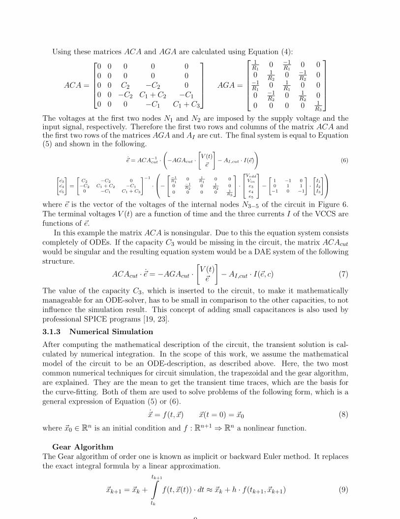
Using these matrices ACA and AGA are calculated using Equation (4):

ACA =

0 0 0 0 00 0 0 0 00 0 C2 −C2 00 0 −C2 C1 + C2 −C1

0 0 0 −C1 C1 + C3

AGA =

1R1

0 −1R1

0 0

0 1R2

0 −1R2

0−1R1

0 1R1

0 0

0 −1R2

0 1R2

0

0 0 0 0 1R3

The voltages at the first two nodes N1 and N2 are imposed by the supply voltage and theinput signal, respectively. Therefore the first two rows and columns of the matrix ACA andthe first two rows of the matrices AGA and AI are cut. The final system is equal to Equation(5) and shown in the following.

~e = ACA−1cut ·

(−AGAcut ·

[V (t)

~e

]−AI,cut · I(~e)

)(6)

[e3e4e5

]=

[C2 −C2 0−C2 C1 + C2 −C1

0 −C1 C1 + C3

]−1

·

−−1

R10 1

R10 0

0 −1R2

0 1R2

0

0 0 0 0 1R3

·Vvdd

Vin

e3e4e5

− [ 1 −1 00 1 1−1 0 −1

]·

[I1I2I3

]where ~e is the vector of the voltages of the internal nodes N3−5 of the circuit in Figure 6.The terminal voltages V (t) are a function of time and the three currents I of the VCCS arefunctions of ~e.

In this example the matrix ACA is nonsingular. Due to this the equation system consistscompletely of ODEs. If the capacity C3 would be missing in the circuit, the matrix ACAcut

would be singular and the resulting equation system would be a DAE system of the followingstructure.

ACAcut · ~e = −AGAcut ·[V (t)~e

]− AI,cut · I(~e, c) (7)

The value of the capacity C3, which is inserted to the circuit, to make it mathematicallymanageable for an ODE-solver, has to be small in comparison to the other capacities, to notinfluence the simulation result. This concept of adding small capacitances is also used byprofessional SPICE programs [19, 23].

3.1.3 Numerical Simulation

After computing the mathematical description of the circuit, the transient solution is cal-culated by numerical integration. In the scope of this work, we assume the mathematicalmodel of the circuit to be an ODE-description, as described above. Here, the two mostcommon numerical techniques for circuit simulation, the trapezoidal and the gear algorithm,are explained. They are the mean to get the transient time traces, which are the basis forthe curve-fitting. Both of them are used to solve problems of the following form, which is ageneral expression of Equation (5) or (6).

~x = f(t, ~x) ~x(t = 0) = ~x0 (8)

where ~x0 ∈ Rn is an initial condition and f : Rn+1 ⇒ Rn a nonlinear function.

Gear AlgorithmThe Gear algorithm of order one is known as implicit or backward Euler method. It replacesthe exact integral formula by a linear approximation.

~xk+1 = ~xk +

tk+1∫tk

f(t, ~x(t)) · dt ≈ ~xk + h · f(tk+1, ~xk+1) (9)

9

where k is the index of the current time step and h is the time step size. As the solution atthe next time step ~xk+1 is implicit, it has to be calculated iteratively. Therefore an initialguess for the solution at the next time step ~x 0

k+1 is used. The formula

~x o+1k+1 = ~xk + h · f(tk+1, ~x

ok+1), (10)

where o is the index of the current number of iteration, is calculated multiple times, untilthe change

4~xk+1 = ~x o+1k+1 − ~x

ok+1 (11)

is smaller than a specified bound. Then the procedure repeats for the next time step k. Afterthe calculation of the second and third time step, some solvers use higher order formulas ofthe Gear algorithm. In difference to the backward Euler method, shown in Equation (9) and(10), this algorithms considers also the states of former time points. These techniques areexplained in detail in [17, 18].

Trapezoidal AlgorithmThe Trapezoidal algorithm is the default algorithm used in SPICE [18, 19]. It is also animplicit algorithm. Instead of assuming a rectangle to approximate the integral, it uses atrapezoid, as shown in the following formula.

~xk+1 = ~xk +

tk+1∫tk

f(t, ~x(t)) · dt ≈ ~xk +h

2· (f(tk, ~xk) + f(tk+1, ~xk+1)) = ~xk +

h

2· (~xk + ~xk+1)

(12)To get the solution for ~xk+1, also for the Trapezoidal algorithm an iterative method is used.The formula to repeat, to find the solution at the next time step, is shown in the following.

~x o+1k+1 = ~xk +

h

2· (f(tk, ~xk) + f(tk+1, ~x

ok+1)) (13)

where o and k are the indices of the current iteration and the current time step, respectively.The initial guess in each time step is usually calculated by the forward Euler method.

~x 0k+1 = ~xk + h · f(tk, ~xk) (14)

This combination of forward Euler and Trapezoidal method is known as Heun’s method.Advanced numerical ODE-solver, as they are used in SPICE or MATLAB, work with avariable time step h. The control of the time step is explained in detail in [17, 18].

3.2 Model Order Reduction

This section briefly explains Krylov MOR techniques. First, the MOR for linear systems isexplained. Then, an approach for the MOR for nonlinear systems, which combines singularvalue decomposition (SVD) and a Krylov algorithm to elaborate a projection matrix, isshown. This is the approach, which also will be used in the presented model generationmethodology in Chapter 5 and for the applications in Chapter 6.

3.2.1 Subspace Methods for Linear Systems

For linear systems, like RC, RL or RLC-circuits, the system description in form of the statespace is shown in the following.

x = A · x+B · uy = C · x

(15)

10

where y ∈ Ro, x ∈ Rn, u ∈ Rp, A ∈ Rn×n, B ∈ Rn×p, and C ∈ Ro×n. MOR will replacethis dynamical system by a system with less state variables, as shown in the following.

˙x = A · x+ B · uy = C ∗ x

(16)

where y ∈ Ro, x ∈ Rq, u ∈ Rp, A ∈ Rq×q, B ∈ Rq×p, C ∈ Ro×q and q < n.Also the reduced system is smaller, it must keep the properties of the original system.

The input-output behaviour of both systems must be similar, which means that the transferfunction of both systems are alike. The system is reduced using its state space matrices.The transfer function can be developed from the state space model, by using Laplace trans-formation, as shown in the following.

1. x = A · x+B · u2. y = C · x

Laplace Transformation ↓3. s ·X(s) = A ·X(s) +B · U(s)

4. Y (s) = C ·X(s)

from 3. s ·X(s)− A ·X(s) = B · U(s)

(s · I − A) ·X(s) = B · U(s)

5. X(s) = (s · I − A)−1 · (B · U(s))

from 4. and 5. Y (s) = C · (s · I − A)−1 · (B · U(s))

G(s) = Y (s) · U(s)−1 = C · (s · I − A)−1 ·B

(17)

where I is the identity matrix. If the system is a single input single output (SISO) sys-tem, the transfer function can be transformed to a fraction of two polynomials using Padeapproximation [9].

G(s) =Y (s)

U(s)=a0 + a1 · s+ a2 · s2 + ...+ an · sn

1 + b1 · s+ b2 · s2 + ...+ bm · sm(18)

Around an expansion point s0 ∈ C this polynomials can be replaced by an infinite powerseries [3] of its moments m, as shown in Equation (19). To find a reduced description of thetransfer function, its most significant moments have to be computed. The transfer functionof the reduced system G(s) just consists of the q most significant moments of the originaltransfer function G(s).

G(s) = m0 +m1 · (s− s0) +m2 · (s− s0)2 +m3 · (s− s0)3 + ...

G(s) = m0 +m1 · (s− s0) +m2 · (s− s0)2 + ...+mq · (s− s0)q(19)

One method, to find the moments, is the Arnoldi algorithm. It will compute a matrixV ∈ Rn×q, where q is the number of the moments, and V · V T = I. The matrix V consistsof the moment vectors:

V (B, A) = spanB, A ·B, ..., Aq−1 ·B = [V1, V2, ..., Vq].

The Arnoldi algorithm, shown in the following, is an iterative algorithm. It computes theeigenvalues and eigenvectors of a matrix, to get an orthogonal basis for a Krylov subspace.

11

Algorithm Arnoldi: [A, B, q]→ V

V1 = b||b||

for i = 1 to q dov = 〈A, Vi〉for j = 1 to q doHj,i = 〈V, v〉v = v −Hj,i · Vj

end forHi+1,i = ||v||Vi+1 = v

Hi+1,i

end for

The matrix of interest is the system matrix A. The start vector for the iteration is thevector B. q is the number of iterations, which is equal to the number of the columns of thematrix V , which the algorithm will compute. It is proven, e.g., in [24], that the momentmatching using Arnoldi algorithm, will keep the q most significant moments of the transferfunction, as long as it does not break down. This would be the case, if q reaches the rank ofmatrix A. That means, that the transfer function of the reduced model, which is calculatedas shown in the following, has the same first q moments as the original system. To computethe reduced model in the subspace, the matrix V is used, which is the output of the Arnoldialgorithm.

A = V T · A , B = V T ·B , C = C · V

Another well known algorithm to find a Krylov subspace, by computing the eigenvaluesand eigenvectors of the matrix A, is the Lanczos algorithm [3]. An approach to makethe Arnoldi algorithm working for multi input multi output (MIMO) systems is the globalArnoldi algorithm, which is shown as an extension of the standard Arnoldi algorithm in [25].

3.2.2 Nonlinear Systems

Also, there are a lot of parts in electronic circuits, which can be modelled by a linear system,the most circuits are nonlinear. For those systems a reduction is not as straightforward asfor linear systems. A method to find a projection basis for a nonlinear state space model,using Arnoldi algorithm and SVD, is presented in the following. It is similar to the trajectorypiecewise MOR, which is presented in [4, 5, 26, 27]. It is shown, how the reduced nonlinearsystem is simulated, using piecewise linear models.A nonlinear model has the general description

x = f(x, u(t))

y = g(x),(20)

where x ∈ Rn are the state variables of the system, u ∈ Rp and y ∈ Ro the input and outputvector of the system and f : Rn+p → Rn and g : Rn → Ro are nonlinear functions.This model is transformed to a piecewise model of k linear systems, using the simulationtraces of a former simulation of the system. For the linearisation of the system around thek linearisation points xL, the Jacobian matrices Jx and Ju of f at these points are used.

12

Jx contains all first derivatives of f regarding to the state variables, while Ju contains thederivatives to the input signals. A method to find the linearization points is shown in detailin Chapter 5.

The function f of Equation (20) is replaced by the following linear expression, which isequal to the Taylor polynomial of order 1 of f .

x = xL,i + Jx,i · (x− xL,i) + Ju,i · uxL,i = min

xL,i

(||xL,1 − x||, ||xL,2 − x||, ..., ||xL,k − x||) (21)

where Jx ∈ Rn×n, Ju ∈ Rn×p and i is the index to identify the corresponding linear system,which is the system, whose development point xL,i is the closest to the current state x.To find a projection matrix, the Arnoldi algorithm is applied to all system matrices Ai tofind the k eigenvector-matrices Vi. Again, each matrix Vi contains the q most significanteigenvectors of the corresponding matrix A. The final projection matrix U is a product ofthe SVD of the combination of all the matrices Vi. The SVD is already implemented inMATLAB. The other two matrices resulting from the SVD are not used.

(U, P,O) = SV D (V1 ∪ V2 ∪ ... ∪ Vk)

Matrix U is used as projection matrix. It transforms the model, shown in Equation (21), tothe reduced state space model shown in the following.

z = zi + Ai · (z − zi) +Bi · uzi = min

zi(||z1 − z||, ||z2 − z||, ..., ||zk − z||) (22)

whereA = UT · Jx · UB = UT · Juzi = UT · xL,i

(23)

For a numerical simulation of the dynamical system, the initial condition is projected tothe reduced state space. Then, at each time step tk of the numerical solution of the reducedsystem, the current linear system is selected by searching for the closest linearization point zito the current state z(t). Once the simulation is finished, the time traces of the reduced statespace variables are transformed back to the original state space and provide an approximationof the solution in the original state space.

x(t) = U · z(t) (24)

4 Curve-Fitting of Analog Circuit Simulation Traces

The focus of this chapter is to identify successful methods for the curve-fitting of analogcircuits. The function system, which is the desired output of the curve-fitting procedure isan ODE-system. It can be used instead of the original system, to describe the behaviour ofthe analog circuit. At this point it is necessary to differentiate between linear and nonlinearsystems, as the effort for the curve-fitting and the additionally required information are quitedifferent. In case of a linear system the procedure shown in Section 4.1 can be used to findthe system description, if the parameters of the original circuit are unknown. For nonlinearsystems, the procedure shown in Section 4.2 is helpful if the active device models, which

13

are used by the original simulation, are to complicated and should be replaced by simplermodels.

For both linear and nonlinear systems, the curves, which are under the focus of thecurve-fitting, are the time derivatives of the circuits state variables. An approximation ofthese time derivatives is calculated using the time traces themselves.

~x ≈(4~x4t

)sampl

(25)

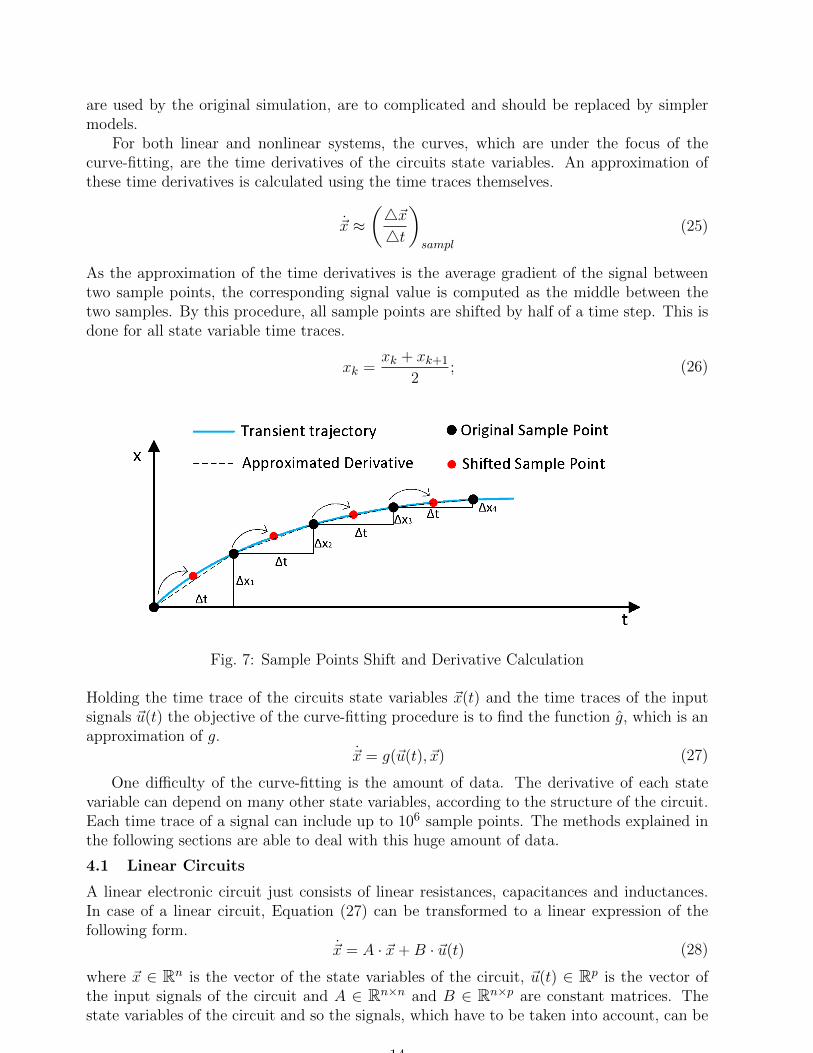
As the approximation of the time derivatives is the average gradient of the signal betweentwo sample points, the corresponding signal value is computed as the middle between thetwo samples. By this procedure, all sample points are shifted by half of a time step. This isdone for all state variable time traces.

xk =xk + xk+1

2; (26)

Fig. 7: Sample Points Shift and Derivative Calculation

Holding the time trace of the circuits state variables ~x(t) and the time traces of the inputsignals ~u(t) the objective of the curve-fitting procedure is to find the function g, which is anapproximation of g.

~x = g(~u(t), ~x) (27)

One difficulty of the curve-fitting is the amount of data. The derivative of each statevariable can depend on many other state variables, according to the structure of the circuit.Each time trace of a signal can include up to 106 sample points. The methods explained inthe following sections are able to deal with this huge amount of data.

4.1 Linear Circuits

A linear electronic circuit just consists of linear resistances, capacitances and inductances.In case of a linear circuit, Equation (27) can be transformed to a linear expression of thefollowing form.

~x = A · ~x+B · ~u(t) (28)

where ~x ∈ Rn is the vector of the state variables of the circuit, ~u(t) ∈ Rp is the vector ofthe input signals of the circuit and A ∈ Rn×n and B ∈ Rn×p are constant matrices. Thestate variables of the circuit and so the signals, which have to be taken into account, can be

14

identified using the MNA method, shown in Section 3.1.2. To prepare the curve-fitting forthe identification of the matrices A and B, Equation (28) is transcribed to:

~x =[B A

]·[~u(t)~x

]= J ·

[~u(t)~x

](29)

where J ∈ Rn×(n+p) is the Jacobian matrix of the system. This matrix contains all firstderivatives of the state variables to each other and to the input signals.

J =

∂x1

∂u1

∂x1

∂u2... ∂x1

∂up

∂x1

∂x1

∂x1

∂x2... ∂x1

∂xn∂x2

∂u1

∂x2

∂u2... ∂x2

∂up

∂x2

∂x1

∂x2

∂x2... ∂x2

∂xn

......

......

......

∂xn

∂u1

∂xn

∂u2... ∂xn

∂up

∂xn

∂x1

∂xn

∂x2... ∂xn

∂xn

(30)

For a linear system, the Jacobian is constant and independent from the state variables. Itis a complete description of the dynamical system. To calculate all elements of J with themean of the time simulation traces, n linear systems are developed, which each correspondsto one line of the Jacobian matrix and one derivative of a state variable. Using this approach,the elements of J are calculated row by row. The equation system for the nth state variableconsists of equations of the following form.

xn,k = Jn,1 · u1,k + ...+ Jn,p · up,k + Jn,p+1 · x1,k + ...+ Jn,p+n · xn,k (31)

where k is the number of sample points. Every sample point will add an equation to thelinear system. As the number of sample points of a numerical simulation is normally muchlarger than the number of state variables, the equation system is overdetermined. Herean overdetermined system is necessary for a proper solution, as all equations are just anapproximation (Equation 25).

Developing equations (31) for all sample points, the complete system is found.

b = A · c (32)

where b =

xn,1xn,2

...xn,k

, A =

~uT1 ~xT1~uT2 ~xT2...

...~uTk ~xTk

and c =

Jn,1Jn,2

...Jn,p+n

.

The best solution of this overdetermined system is expressed as a least squares prob-lem. The values copt which minimize the square of residuals between the samples and thelinear function for all time steps, must be calculated.

copt = minc

k∑a=1

(resa)2 = minc

(A · c− b)2 (33)

Two techniques to solve (33) are shown in the following.

4.1.1 Normal Equations

To find the minimum of the least squares, the scalar product is expanded

(A · c− b)2 = (A · c− b)T · (A · c− b)= cT · AT · A · c− 2 · cT · AT · b− bT · b

(34)

15

and its derivative regarding c is set to zero, to calculate the values of c, which minimize thesum of the squares of the residuals.

0 = 2 · AT · A · c− 2 · AT · bc = (AT · A)−1 · AT · b

(35)

Using the original symbols again, for each line n of the matrix J the following equation willcalculate its parameters, by using the k sample points of a former transient simulation.

Jn,1Jn,2

...Jn,p+n

=

[~u1 ~u2 ... ~uk~x1 ~x2 ... ~xk

]·

~uT1 ~xT1~uT2 ~xT2...

...~uTk ~xTk

−1

·[~u1 ~u2 ... ~uk~x1 ~x2 ... ~xk

]·

xn,1xn,2

...xn,k

(36)

4.1.2 QR Decomposition

Another technique, to solve Equation (33), is to use the QR decomposition of the matrix A.QR decomposition will replace the matrix A by an orthogonal matrix Q and a square, uppertriangular matrix R.

A = Q ·RQT ·Q = I

(37)

where I is the identity matrix and A ∈ Rk×(n+p) , Q ∈ Rk×(n+p) and R ∈ R(n+p)×(n+p).Using this decomposition we can rewrite Equation (32) to find c.

b = Q ·R · cQT · b = R · c

c = R−1 ·QT · b(38)

The QR decomposition algorithm is available as a function in MATLAB with the followingcommand.

[Q,R]=qr(A);

4.1.3 Example

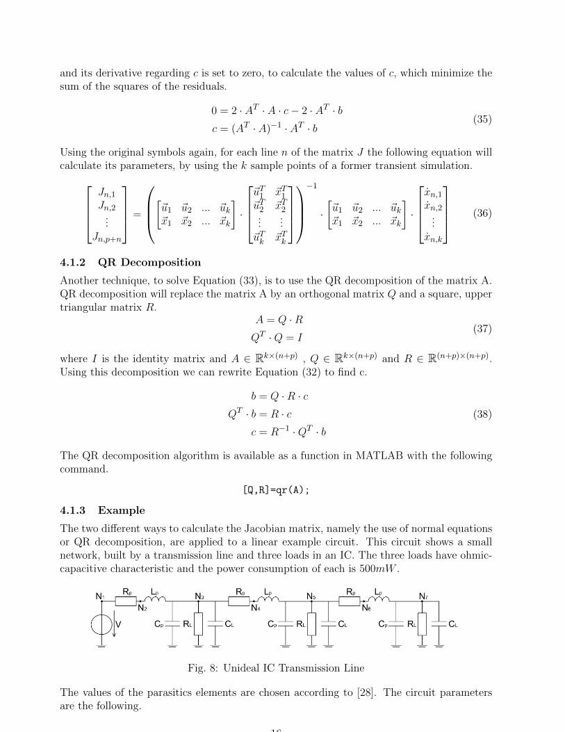
The two different ways to calculate the Jacobian matrix, namely the use of normal equationsor QR decomposition, are applied to a linear example circuit. This circuit shows a smallnetwork, built by a transmission line and three loads in an IC. The three loads have ohmic-capacitive characteristic and the power consumption of each is 500mW .

Fig. 8: Unideal IC Transmission Line

The values of the parasitics elements are chosen according to [28]. The circuit parametersare the following.

16

RP = 1Ω , LP = 25fH , CP = 1pF , RL = 50Ω , CL = 0.5nF

The state variables vector of this circuit is built by the node voltages with capacitive couplingand the currents through inductances. The only input signal is the supply voltage.

~xT =[e3 e5 e7 iL1 iL2 iL3

], u(t) = V (t)

Using the MNA approach provided in Section 3.1.2 the circuit equation system is shown bythe following linear system.

~x =

0 −1RL·(CP +CL)

0 0 1CP +CL

−1CP +CL

0

0 0 −1RL·(CP +CL)

0 0 1CP +CL

−1CP +CL

0 0 0 −1RL·(CP +CL)

0 0 1CP +CL

1Lp

−1LP

0 0 −Rp

LP0 0

0 1Lp

−1LP

0 0 −Rp

LP0

0 0 1Lp

−1LP

0 0 −Rp

LP

·[~u(t)~x

]

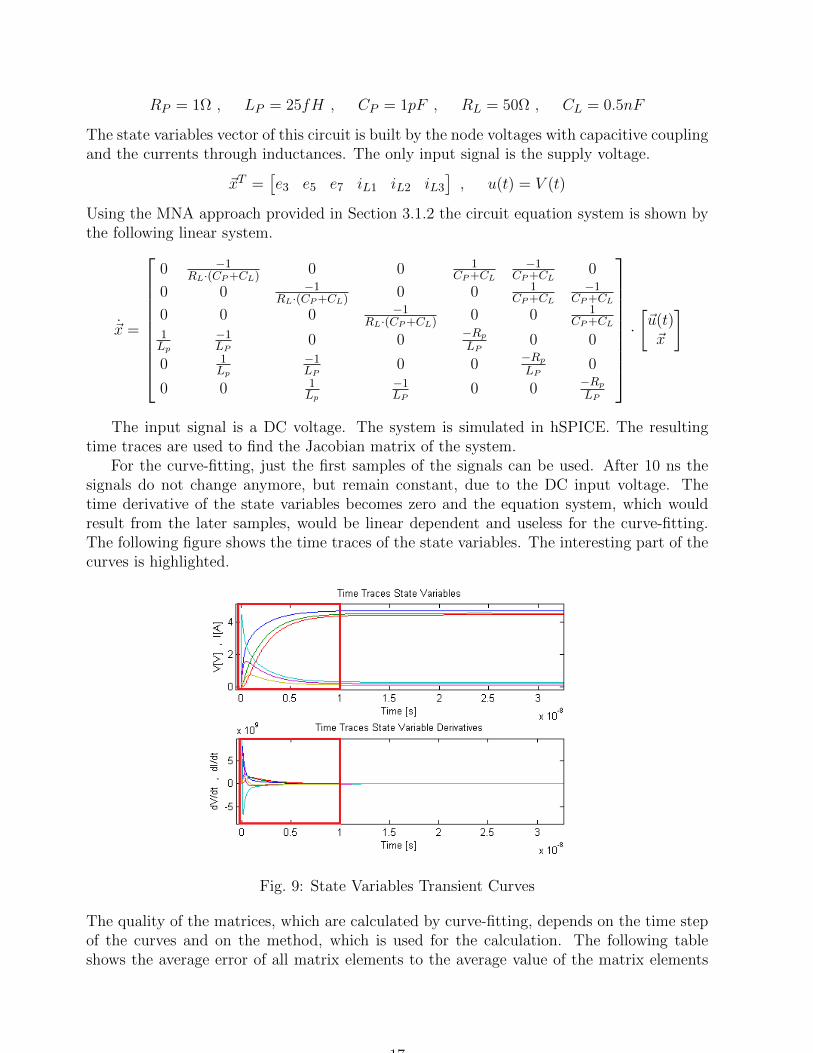
The input signal is a DC voltage. The system is simulated in hSPICE. The resultingtime traces are used to find the Jacobian matrix of the system.

For the curve-fitting, just the first samples of the signals can be used. After 10 ns thesignals do not change anymore, but remain constant, due to the DC input voltage. Thetime derivative of the state variables becomes zero and the equation system, which wouldresult from the later samples, would be linear dependent and useless for the curve-fitting.The following figure shows the time traces of the state variables. The interesting part of thecurves is highlighted.

Fig. 9: State Variables Transient Curves

The quality of the matrices, which are calculated by curve-fitting, depends on the time stepof the curves and on the method, which is used for the calculation. The following tableshows the average error of all matrix elements to the average value of the matrix elements

17

and the maximum error of all elements.

Erroraverage =

n∑i=1

n+p∑j=1

(4Ji,j

Jmean

)size(J)

(39)

Errormax = max

(4Ji,jJmean

)(40)

where size(J) is the total number of elements in the matrix.

Table 1: Jacobian Matrix Quality for Different Methods and Traces

Method Normal Equation QR Decomposition

Traces Time StepSize [s]

1e-14 1e-13 1e-12 1e-11 1e-14 1e-13 1e-12 1e-11

Erroraverage 1.1e-4 1.7e-3 2.1e-3 0.15 4.3e-8 1.6e-3 2.1e-2 0.15

Errormax 1.0e-3 2.0e-2 0.25 1.4 1.8e-7 2.0e-2 0.25 1.4

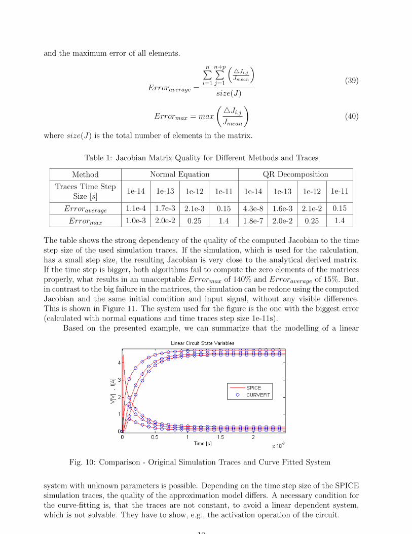
The table shows the strong dependency of the quality of the computed Jacobian to the timestep size of the used simulation traces. If the simulation, which is used for the calculation,has a small step size, the resulting Jacobian is very close to the analytical derived matrix.If the time step is bigger, both algorithms fail to compute the zero elements of the matricesproperly, what results in an unacceptable Errormax of 140% and Erroraverage of 15%. But,in contrast to the big failure in the matrices, the simulation can be redone using the computedJacobian and the same initial condition and input signal, without any visible difference.This is shown in Figure 11. The system used for the figure is the one with the biggest error(calculated with normal equations and time traces step size 1e-11s).

Based on the presented example, we can summarize that the modelling of a linear

Fig. 10: Comparison - Original Simulation Traces and Curve Fitted System

system with unknown parameters is possible. Depending on the time step size of the SPICEsimulation traces, the quality of the approximation model differs. A necessary condition forthe curve-fitting is, that the traces are not constant, to avoid a linear dependent system,which is not solvable. They have to show, e.g., the activation operation of the circuit.

18

4.2 Nonlinear Circuits

After presenting, how a linear system model can be derived, by the use of the transient timetraces, the focus of this section is on nonlinear circuits. In the following, two techniquesare shown, which approximate the mathematical description of a nonlinear circuit by curve-fitting. The first technique, the Vandermode Interpolation Method, tries to fit a curve witha polynomial function, while the second method, the LevenbergMarquardt algorithm, is aleast-squares algorithm, which identifies a set of parameters to minimize the failure betweena guess function and a curve.

4.2.1 Vandermode Interpolation Method

The Vandermode Interpolation method used here is described in [29]. It can approximatecurves of signals, which depend on more than one other signal, what is required in the caseof circuits.

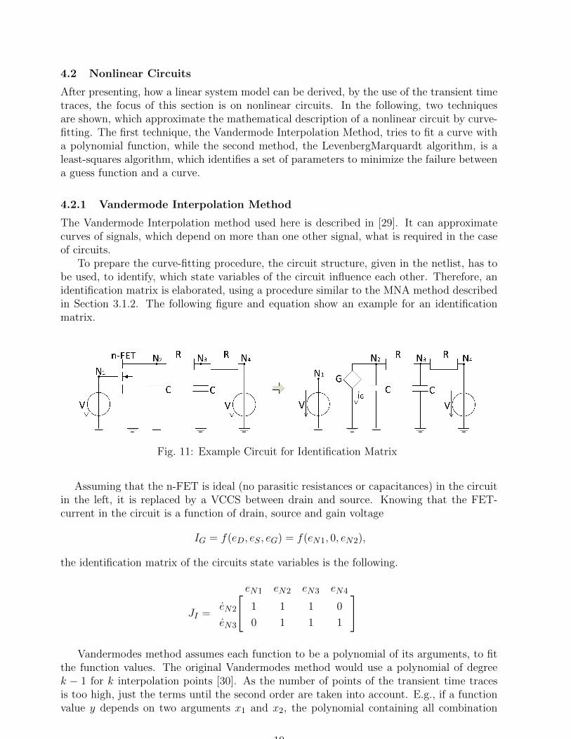
To prepare the curve-fitting procedure, the circuit structure, given in the netlist, has tobe used, to identify, which state variables of the circuit influence each other. Therefore, anidentification matrix is elaborated, using a procedure similar to the MNA method describedin Section 3.1.2. The following figure and equation show an example for an identificationmatrix.

Fig. 11: Example Circuit for Identification Matrix

Assuming that the n-FET is ideal (no parasitic resistances or capacitances) in the circuitin the left, it is replaced by a VCCS between drain and source. Knowing that the FET-current in the circuit is a function of drain, source and gain voltage

IG = f(eD, eS , eG) = f(eN1, 0, eN2),

the identification matrix of the circuits state variables is the following.

JI =

[ eN1 eN2 eN3 eN4

eN2 1 1 1 0

eN3 0 1 1 1

]

Vandermodes method assumes each function to be a polynomial of its arguments, to fitthe function values. The original Vandermodes method would use a polynomial of degreek − 1 for k interpolation points [30]. As the number of points of the transient time tracesis too high, just the terms until the second order are taken into account. E.g., if a functionvalue y depends on two arguments x1 and x2, the polynomial containing all combination

19

until the second order, would look like the following.

y = c1 + c2 · x1 + c3 · x2 + c4 · x21 + c5 · x2

2 + c6 · x1 · x2 + c7 · x21 · x2 + c8 · x1 · x2

2 (41)

At this point the linear equation system is developed using the k sample points of thetransient time traces. The function value y would be the derivative of the state variables,using Equation (25).

y1 = c1 + c2 · x1,1 + c3 · x2,1 + c4 · x21,1 + c5 · x2

2,1 + ...+ c8 · x1,1 · x22,1

y2 = c1 + c2 · x1,2 + c3 · x2,2 + c4 · x21,2 + c5 · x2

2,2 + ...+ c8 · x1,2 · x22,2

...

yk = c1 + c2 · x1,k + c3 · x2,k + c4 · x21,k + c5 · x2

2,k + ...+ c8 · x1,k · x22,k

The linear coefficients c in this polynomial are determined by solving the linear equationsystem, e.g., using the methods explained in the previous section.

This technique has two main drawbacks and is therefore not practical for the curve-fittingof nonlinear circuits. The first reason is that the derivative of all state variables usually de-pend on more than three other signals. The linear systems derived by the Vandermodesmethod will become too large and contain too many coefficients c, even, if just the secondorder polynomial of the arguments is used. The second drawback is the violation of Kirch-hoff’s current law, which results, if this method is applied to complete circuits. If the methodis used as described, the sum of currents in every node would not be zero.

4.2.2 LevenbergMarquardt Algorithm

The Levenberg-Marquardt algorithm is the state of the art for nonlinear curve-fitting tasks[31, 32]. It is implemented in many standard tools like MATLAB, GNU Octave or Mathe-matica. The algorithm is used to identify a set of parameters c = (c1, c2, ..., cn) of a nonlin-ear function y = f(x1, x2, ..., xm, c1, c2, ..., cn) for a given set of points (yi, x1,i, x2,i, ..., xm,i),where i = 1, 2, ..., k [32, 33]. In this section, the algorithm itself is explained and then it isshown, how to get the function guess f , by using the nonlinear electronic circuits netlist.

The problem is to minimize the sum of squares of the residuals between the nonlinearfunction f(xi, c) and the set of points yi.

copt = minc

k∑i=1

(resi)2 = min

c

k∑i=1

(yi − f(xi, c))2 (42)

where xi = (x1,i, x2,i, ..., xm,i).

To find the set copt, the sum of squares of all k points is elaborated in vector form

S(c) = ||Y − f(x, c)||2 (43)

and starting from an initial set of parameters c0 the problem is solved iteratively. At eachiteration it is tried to find a better set of parameters cnew = c+ d. The parameters in d aredetermined in each iteration, as it will lead to a new estimation of the parameters set c. Thesum of squares for the new parameters is calculated as an approximation, as follows.

S(c+ d) ≈ ||Y − f(x, c)− J · d||2 (44)

20

where J is the composition of all Jacobian vectors Ji. The Jacobian vectors Ji contain allderivatives of y = f(x, c) to all parameters c = (c1, c2, ..., cn) at the points (yi, xi, c). Thenthe vector d, which minimizes the sum of squares, is calculated by setting the derivative ofthe sum of squares to d equal to zero.

0 =∂S(c+ d)

∂d=

∂

∂d||Y − f(x, c)− J · d||2

0 =∂

∂d[(Y − f(x, c)− J · d)T · (Y − f(x, c)− J · d)]

0 =∂

∂d[(Y − f(x, c))T · (Y − f(x, c))− 2 · (J · d)T · (Y − f(x, c)) + dT · JT · J · d]

0 = −2 · JT · (Y − f(x, c)) + 2 · JT · J · dJT · J · d = JT · (Y − f(x, c))

(45)

At this point the vector d could be calculated, by solving the linear system, which is reached.This would have the drawback that the parameters d would be too big, if the initial set ofparameters c0 is too far from the optimal solution copt [32]. Due to this the iterative algo-rithm would not converge. The damping factor λ is used to make the algorithm more robustagainst a bad initial guess. It is calculated depending on the change of the sum of squaresS using a trust region method, as explained in detail in [32].

(JT · J + λ · I) · d = JT · (Y − f(x, c)) (46)

The vector of the change of parameters d is in addition modified, using a scaling matrixdiag(JTJ), what again has a positive effect on the convergence and the speed of the algo-rithm [32].

(JT · J + λ · diag(JTJ)) · d = JT · (Y − f(x, c)) (47)

Using this equation, the change of the parameters d is calculated iteratively, until the sizeof d or the change in sum of squares of the residuals is smaller than a defined bound. Thelast set of parameters is a local minimum of the sum of squares.

To elaborate the function f , which will be used as a function guess for the Levenberg-Marquardt algorithm, the MNA method is used, which was presented in Section 3.1.2. Activedevices are replaced by simplified equivalent circuits, which include VCCS with some unde-fined parameters c. The functions of the VCCS will be exponential functions for the VCCSfor diodes and BJTs, while for FETs a piecewise function is used, which contains the linearand quadratic terms of the terminal values. This is shown in detail in Section 5.1.

Using the Levenberg-Marquardt algorithm to curve-fit the transient simulation traces ofthe original circuit, its parameters c are determined. This approach has the advantage thatthe elaborated function guess is close to the analytical function, as all the passive elementvalues are taken from the netlist, while the active devices are simplified, but still contain agood function guess. The number of parameters to determine is small, compared to the oneof the Vandermodes interpolation approach.

5 Reduced Model Generation

This Chapter shows how to combine the techniques introduced in Chapters 3 and 4 togenerate reduced circuit models, using the time traces of their SPICE simulation. The

21

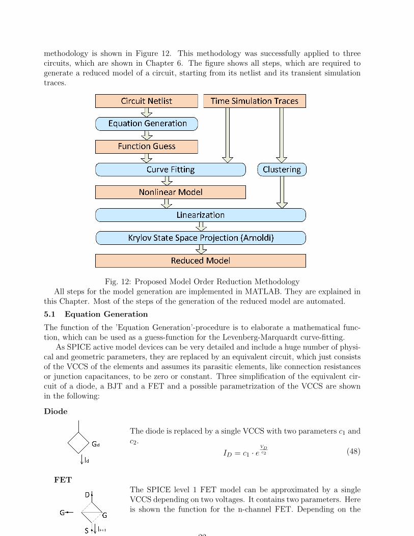
methodology is shown in Figure 12. This methodology was successfully applied to threecircuits, which are shown in Chapter 6. The figure shows all steps, which are required togenerate a reduced model of a circuit, starting from its netlist and its transient simulationtraces.

Fig. 12: Proposed Model Order Reduction MethodologyAll steps for the model generation are implemented in MATLAB. They are explained in

this Chapter. Most of the steps of the generation of the reduced model are automated.

5.1 Equation Generation

The function of the ’Equation Generation’-procedure is to elaborate a mathematical func-tion, which can be used as a guess-function for the Levenberg-Marquardt curve-fitting.

As SPICE active model devices can be very detailed and include a huge number of physi-cal and geometric parameters, they are replaced by an equivalent circuit, which just consistsof the VCCS of the elements and assumes its parasitic elements, like connection resistancesor junction capacitances, to be zero or constant. Three simplification of the equivalent cir-cuit of a diode, a BJT and a FET and a possible parametrization of the VCCS are shownin the following:

Diode

The diode is replaced by a single VCCS with two parameters c1 andc2.

ID = c1 · eVDc2 (48)

FETThe SPICE level 1 FET model can be approximated by a singleVCCS depending on two voltages. It contains two parameters. Hereis shown the function for the n-channel FET. Depending on the

22

operating frequency, the parasitic capacitances have to be added.

IDS =

0 if VGS < c1c2 · 0.5 · (VGS − c1) if VDS > VGS − c1 > 0

c2 · VDS · (VGS − c1 − VDS

2 ) if VDS < VGS − c1(49)

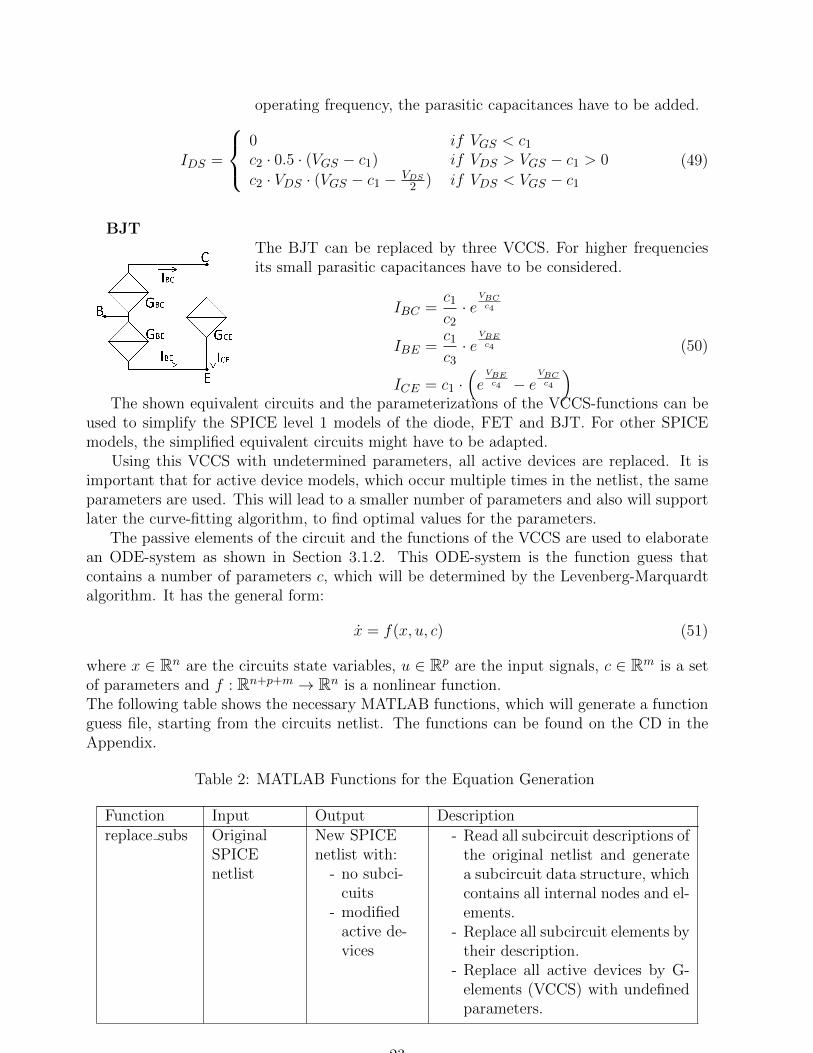
BJTThe BJT can be replaced by three VCCS. For higher frequenciesits small parasitic capacitances have to be considered.

IBC =c1c2· e

VBCc4

IBE =c1c3· e

VBEc4

ICE = c1 ·(e

VBEc4 − e

VBCc4

) (50)

The shown equivalent circuits and the parameterizations of the VCCS-functions can beused to simplify the SPICE level 1 models of the diode, FET and BJT. For other SPICEmodels, the simplified equivalent circuits might have to be adapted.

Using this VCCS with undetermined parameters, all active devices are replaced. It isimportant that for active device models, which occur multiple times in the netlist, the sameparameters are used. This will lead to a smaller number of parameters and also will supportlater the curve-fitting algorithm, to find optimal values for the parameters.

The passive elements of the circuit and the functions of the VCCS are used to elaboratean ODE-system as shown in Section 3.1.2. This ODE-system is the function guess thatcontains a number of parameters c, which will be determined by the Levenberg-Marquardtalgorithm. It has the general form:

x = f(x, u, c) (51)

where x ∈ Rn are the circuits state variables, u ∈ Rp are the input signals, c ∈ Rm is a setof parameters and f : Rn+p+m → Rn is a nonlinear function.The following table shows the necessary MATLAB functions, which will generate a functionguess file, starting from the circuits netlist. The functions can be found on the CD in theAppendix.

Table 2: MATLAB Functions for the Equation Generation

Function Input Output Descriptionreplace subs Original

SPICEnetlist

New SPICEnetlist with:

- no subci-cuits

- modifiedactive de-vices

- Read all subcircuit descriptions ofthe original netlist and generatea subcircuit data structure, whichcontains all internal nodes and el-ements.

- Replace all subcircuit elements bytheir description.

- Replace all active devices by G-elements (VCCS) with undefinedparameters.

23

read netlist New SPICEnetlist with:

- no subci-cuits

- modifiedactivedevices

ElementsStructure inMATLAB

- Read the SPICE netlist and addeach element to a structure inMATLAB.

- For the linear elements (R,L,C)save their values (in Ω, H, F ) andnodes.

- For the G-elements save the func-tion, the controlling nodes andthe connected nodes.

develop MNAmatrices

ElementsStructure

Nodes List,MNA Matri-ces:AGA, ACA,AI

- Elaborate the numerical matrices,by using the information aboutthe linear elements and the con-nection nodes.

- Elaborate a nodes list.

develop I ElementsStructure

String Array I - Development of a string array,which consists of the functions ofthe VCCSs.

develop parafile

MNA Matri-ces, NodesList, StringArray I

Function GuessFile

- Development of a MATLAB file,which contains the function guessfor the whole circuit and whichcan be called from the curve-fitting algorithm.

5.2 Curve-Fitting

For the curve-fitting, the Levenberg-Marquard algorithm described in Section 4.2.2 is used.This algorithm is available in MATLAB as an option of the function

lsqcurvefit.

The SPICE simulation traces of the state space signals are read form the SPICE output fileby a MATLAB function. They are arranged, to correspond to the state variables of the guessfunction. For a successful curve-fitting, the time traces have to show the transient behaviourof the circuit, which means, they have to change over time. If a signal stays constant, itsderivative will be zero and these sample points cannot be used for the curve-fitting. Toprepare a good curve-fitting, regions in the time traces, where a signal has a high gain ordecline, have to be chosen instead of regions, where the signal stays constant.

The Levenberg-Marquard algorithm will return the set of parameters c, which is theclosest minimum of the sum of the residuals to the initial guess c0. To find the best set ofparameters copt, it can be necessary to try systematically different sets of input parameters.As the curve-fitting algorithm will also return the sum of the residuals, which remains forthe calculated set copt, it is easy to identify the best set of parameters.

The output of the curve-fitting is a set of parameters, which will give an approximatedODE-description of the circuits state variables. It will transform Equation (51) to thenonlinear model of the circuit.

x = f(x, u) (52)

where x ∈ Rn are the circuits state variables, u ∈ Rp are the input signals and f : Rn+p →Rn is a nonlinear function.

24

5.3 Linearization and State Space Transformation

This section explains how the MOR technique for nonlinear dynamical systems, which wasshown in Section 3.2.2, is applied in the generation of reduced analog circuit models, withinthe methodology.

The time traces of the SPICE transient simulation are not only used to find a simplifiedODE-function, but also for the piecewise linearization of the nonlinear system. The samplepoints of the trajectories are clustered by the kmeans algorithm into a predefined number kof clusters. For n state variables the algorithm will start from an initial set of k points inRn, which can be random or user-defined and which are used as initial cluster center points.Iteratively the algorithm will combine all points, which are close to each other in one cluster.Therefore, in each iteration the points are assigned to the cluster, whose center is the closestto them and the new cluster center points are calculated from all points into the particularcluster. The algorithm stops, when there is no change in the clusters anymore, or when adefined maximum number of iterations is done [34].

The determination of the number of linearization points is one important issue for theautomation of the MOR of nonlinear systems. It is known, that a main factor for the numberof linearization points is the number of state variables. Nevertheless, until now the numberof necessary linearization points cannot be determined automatically, as it also depends onfactors like the operation area of the circuit, the existence of sharp flanks in the input signaland the structure of the circuit. To get a fast reduced model, it is necessary to determinethe number of clusters, which is high enough to transform it from a nonlinear to a piecewiselinear system as shown in Section 3.2.2. But also the number has to be small enough, tonot slow down the simulation, as with a high number of piecewise systems the estimationof the proper system, in each time step of the numerical simulation, would be more timeconsuming.

After the k linearization points xL are determined by using the sample points, the non-linear ODE-system is linearized using a numerical differentiation function in MATLAB [35].This function will elaborate the Jacobean matrix of the ODE-system at each linearizationpoint.

Holding the piecewise linear approximation, the system state space is reduced using theArnoldi algorithm and SVD, as described in Sections 3.2.1 and 3.2.2. The number of statevariables in the reduced state space is chosen as low as possible, to get a high speedup, butguarantee a good model quality.

5.4 Reduced Model Quality

In this section the requirements on a reduced model are discussed. There are two mainexpectations on the reduced model.

It is required essentially that the reduced model approximates the input-output behaviourof the original model precisely. The reduced model must keep the input sensitivity of theoriginal model for all possible input signals, or at least for a big range of input signals, tomake it useable in practice. To validate the input-output behaviour, both the original andthe reduced model, have to be simulated with the same input signals. The error of theoutput signal, which is given in the next chapter for three example circuit simulations, is

25

calculated, using the following equation.

error =

no∑i=1

Tsim∫0

xo,i(t) dt−Tsim∫0

xo,i(t) dt

Tsim∫0

xo,i(t) dt

(53)

where Tsim is the simulation time, no is the number of output signals, xo,i(t) are the timetraces of the output signals of the original model simulation and xo(t) are the output signaltime traces of the simulation of the reduced model transformed back to the original statespace.

The second criteria is the speedup, which is reached, if the reduced model is used insteadof the original model. The speed of the simulation is mainly influenced by the followingeffects. The first factor is the numerical algorithm itself. To have comparable results, thesame backward differentiation algorithm in MATLAB is used for both, the original and thereduced model simulation. The second factor is the number of calculations per timestep.The reduced model requires less steps than the original, as the number of variables to cal-culate is smaller. But the determination of the closest linearization point, which is donein every time step in the simulation of the reduced model, is time consuming. The thirdimportant factor is the number of timesteps. As all advanced solvers control their internalstep size independently from the user, by ensuring, that the local error is in a defined range,the user does not influence the number of steps. For both simulations the same local errorbound is used, also this might force the reduced model simulation to slow down, becauseof a smaller time step size. To measure the speedup in the following section, we comparethe computation time of the original model to the one of the reduced model, when they aresimulated in MATLAB. The duration is not compared to the SPICE simulation time, asit does not use the same integration algorithm and time step control. The original modelin MATLAB is an MNA model, where the VCCSs of the active devices are using detailedparameters, similar to the level 1 models in SPICE.

The speedup given for the applications in Chapter 6 is gained through model simplifica-tion, linearization and reduction.

6 Applications

In this Chapter the proposed methodology is applied to three circuits, namely a voltagecontrolled oscillator (VCO), a two stage operational amplifier (OA) and a frequency divider.It is shown, that the generated reduced models are simulated much faster than the originalmodels, while the error due to the reduction stays small. The speedup, shown for eachcircuit, compares the simulation time in MATLAB for a circuit model, using a transistormodel similar to SPICE level 1 model, and the reduced model, which was generated, usingcurve-fitting of the SPICE simulation traces, and state space transformation.

The simulations were executed on a machine with an ’Intel core i7’ CPU, 2.8 GHz and24 GB of RAM.

6.1 Voltage Controlled Oscillator

The VCO is a widely used device, which provides a rectangle output voltage, whose fre-quency is controlled by its analog input voltage. VCOs are utilized wherever an adaptiveclock-signal is required, e.g., in PLLs. The shown VCO is realized as a ring oscillator of anuneven number of inverters. The delay time of the inverters and so the oscillating frequency

26

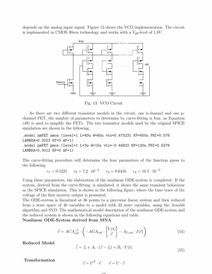
depends on the analog input signal. Figure 13 shows the VCO implementation. The circuitis implemented in CMOS 90nm technology and works with a Vdd-level of 1.8V .

Fig. 13: VCO Circuit

As there are two different transistor models in the circuit, one n-channel and one p-channel FET, the number of parameters to determine by curve-fitting is four, as Equation(49) is used to simplify the FETs. The two transistor models used by the original SPICEsimulation are shown in the following.

.model nmFET nmos (level=1 L=40u W=80u vto=0.475231 KP=450u PHI=0.576

LAMBDA=0.0023 KF=0 AF=1)

.model pmFET pmos (level=1 L=3u W=15u vto=-0.44922 KP=120u PHI=0.5276

LAMBDA=0.0012 KF=0 AF=1)

The curve-fitting procedure will determine the four parameters of the function guess tothe following.

c1 = 0.5225 c2 = 7.2 · 10−4 c3 = 0.6416 c4 = 10.5 · 10−4

Using these parameters, the elaboration of the nonlinear ODE-system is completed. If thesystem, derived from the curve-fitting, is simulated, it shows the same transient behaviouras the SPICE simulation. This is shown in the following figure, where the time trace of thevoltage of the first inverter output is presented.The ODE-system is linearized at 36 points to a piecewise linear system and then reducedfrom a state space of 46 variables to a model with 33 state variables, using the Arnoldialgorithm and SVD. The mathematical model description of the nonlinear ODE-system andthe reduced system is shown in the following equations and table.Nonlinear ODE-System derived from MNA

~e = ACA−1cut ·

(−AGAcut ·

[V (t)~e

]− AI,cut · I(~e)

)(54)

Reduced Model~z = ~zi + Ai · (~z − ~zi) +Bi · V (t)

(55)

Transformation~z = UT · ~e ~e = U · ~z

27

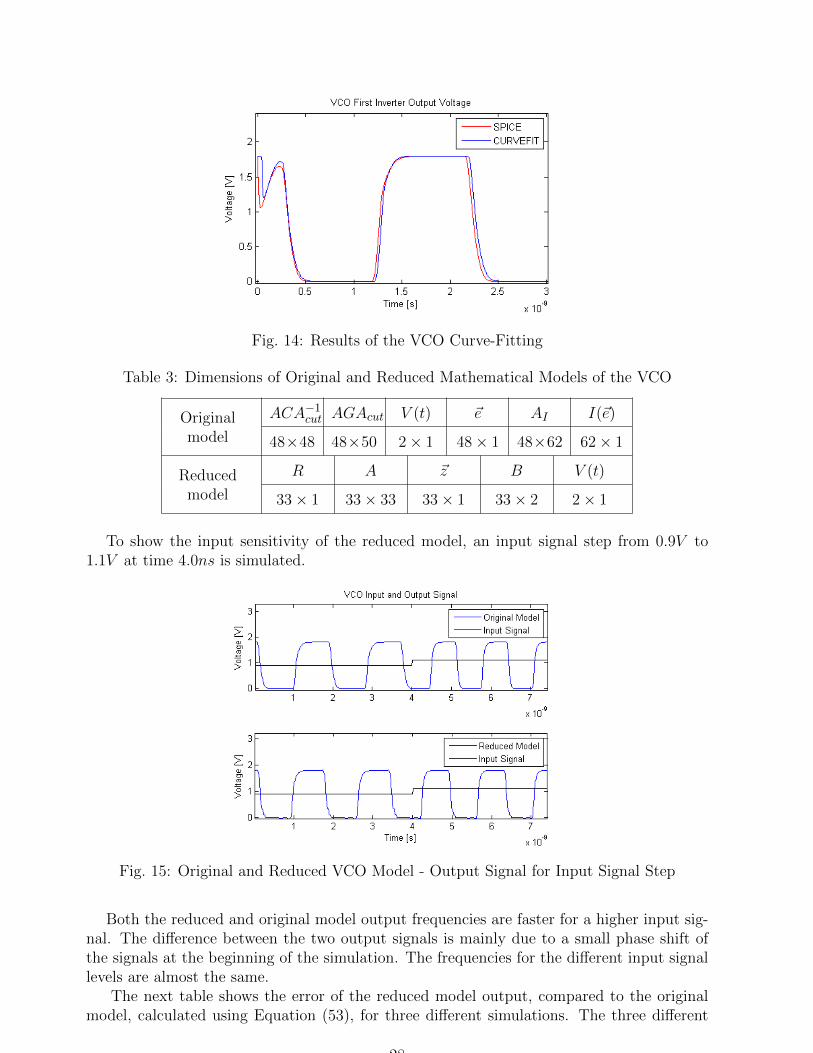
Fig. 14: Results of the VCO Curve-Fitting

Table 3: Dimensions of Original and Reduced Mathematical Models of the VCO

Originalmodel

ACA−1cut AGAcut V (t) ~e AI I(~e)

48×48 48×50 2× 1 48× 1 48×62 62× 1

Reducedmodel

R A ~z B V (t)

33× 1 33× 33 33× 1 33× 2 2× 1

To show the input sensitivity of the reduced model, an input signal step from 0.9V to1.1V at time 4.0ns is simulated.

Fig. 15: Original and Reduced VCO Model - Output Signal for Input Signal Step

Both the reduced and original model output frequencies are faster for a higher input sig-nal. The difference between the two output signals is mainly due to a small phase shift ofthe signals at the beginning of the simulation. The frequencies for the different input signallevels are almost the same.

The next table shows the error of the reduced model output, compared to the originalmodel, calculated using Equation (53), for three different simulations. The three different

28

simulations are using different reduced models.

Table 4: VCO Simulation Results

Input SignalSimulated

TimeSimulation Time [s] Speedup Error

[V ] [ns] Org. Red. [10−2]

const. 1.2 3.00 5.57 1.60 3.47 0.97

const. 0.9 3.00 4.05 1.91 2.12 0.75

step 0.9 to 1.1 7.50 11.4 3.78 3.01 0.64

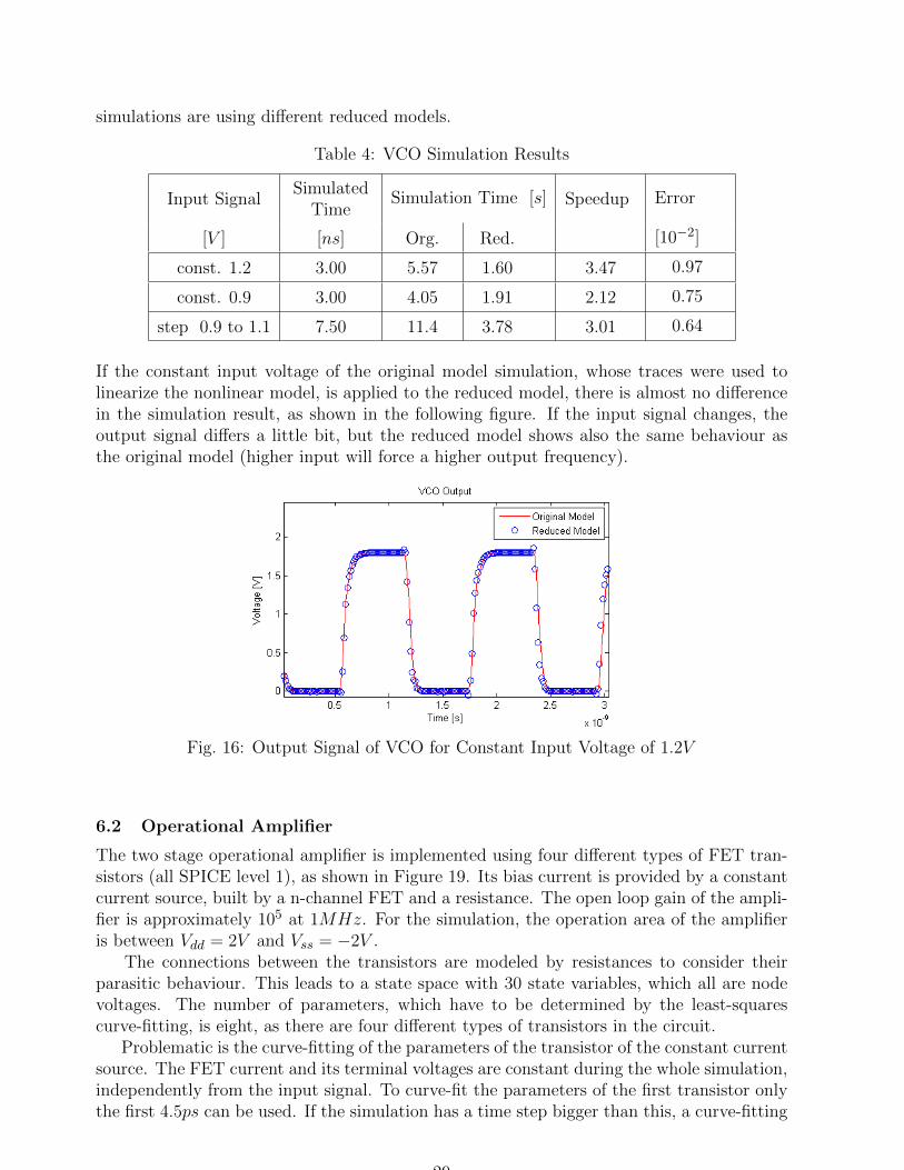
If the constant input voltage of the original model simulation, whose traces were used tolinearize the nonlinear model, is applied to the reduced model, there is almost no differencein the simulation result, as shown in the following figure. If the input signal changes, theoutput signal differs a little bit, but the reduced model shows also the same behaviour asthe original model (higher input will force a higher output frequency).

Fig. 16: Output Signal of VCO for Constant Input Voltage of 1.2V

6.2 Operational Amplifier

The two stage operational amplifier is implemented using four different types of FET tran-sistors (all SPICE level 1), as shown in Figure 19. Its bias current is provided by a constantcurrent source, built by a n-channel FET and a resistance. The open loop gain of the ampli-fier is approximately 105 at 1MHz. For the simulation, the operation area of the amplifieris between Vdd = 2V and Vss = −2V .

The connections between the transistors are modeled by resistances to consider theirparasitic behaviour. This leads to a state space with 30 state variables, which all are nodevoltages. The number of parameters, which have to be determined by the least-squarescurve-fitting, is eight, as there are four different types of transistors in the circuit.

Problematic is the curve-fitting of the parameters of the transistor of the constant currentsource. The FET current and its terminal voltages are constant during the whole simulation,independently from the input signal. To curve-fit the parameters of the first transistor onlythe first 4.5ps can be used. If the simulation has a time step bigger than this, a curve-fitting

29

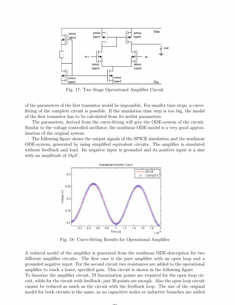
Fig. 17: Two Stage Operational Amplifier Circuit

of the parameters of the first transistor would be impossible. For smaller time steps, a curve-fitting of the complete circuit is possible. If the simulation time step is too big, the modelof the first transistor has to be calculated from its netlist parameters.

The parameters, derived from the curve-fitting will give the ODE-system of the circuit.Similar to the voltage controlled oscillator, the nonlinear ODE-model is a very good approx-imation of the original system.

The following figure shows the output signals of the SPICE simulation and the nonlinearODE-system, generated by using simplified equivalent circuits. The amplifier is simulatedwithout feedback and load. Its negative input is grounded and its positive input is a sinewith an amplitude of 18µV .

Fig. 18: Curve-fitting Results for Operational Amplifier

A reduced model of the amplifier is generated from the nonlinear ODE-description for twodifferent amplifier circuits. The first case is the pure amplifier with an open loop and agrounded negative input. For the second circuit two resistances are added to the operationalamplifier to reach a lower, specified gain. This circuit is shown in the following figure.To linearize the amplifier circuit, 79 linearization points are required for the open loop cir-cuit, while for the circuit with feedback, just 30 points are enough. Also the open loop circuitcannot be reduced as much as the circuit with the feedback loop. The size of the originalmodel for both circuits is the same, as no capacitive nodes or inductive branches are added

30

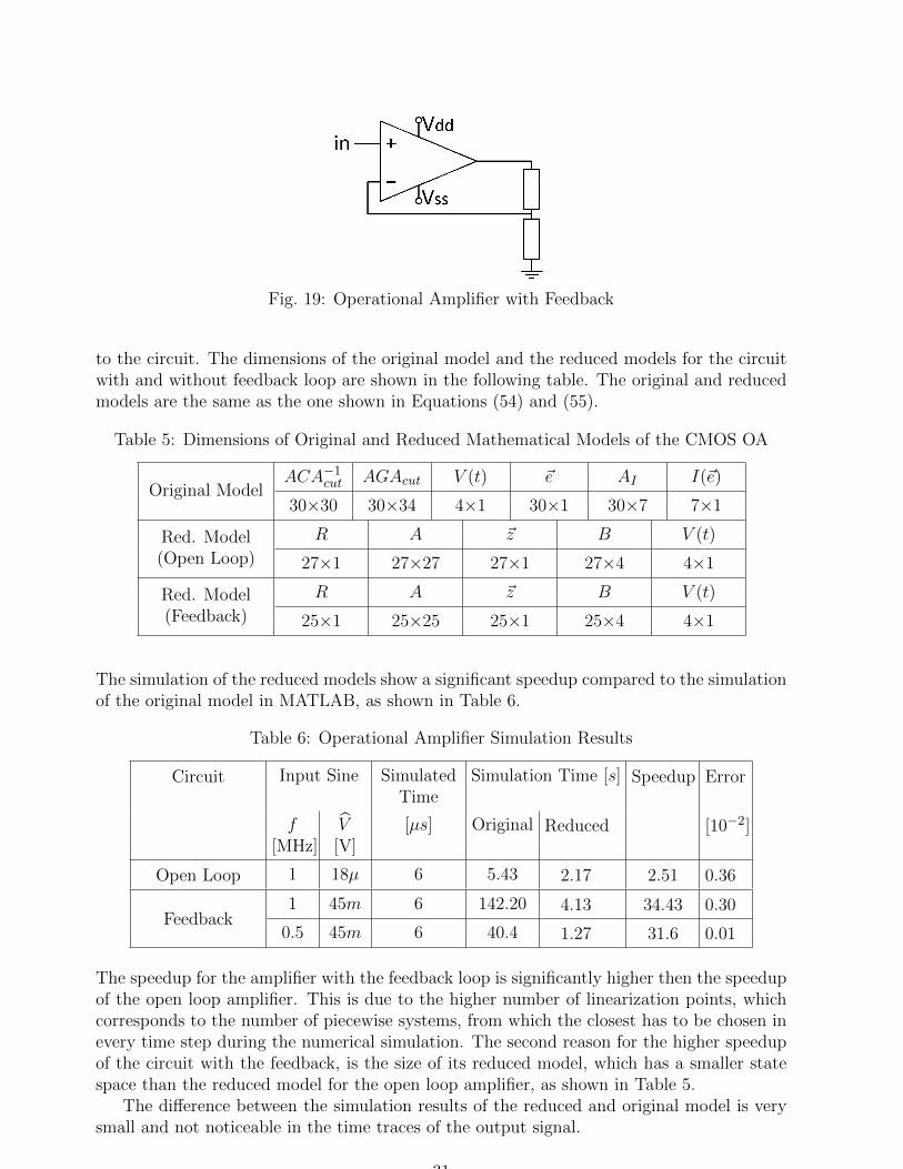
Fig. 19: Operational Amplifier with Feedback

to the circuit. The dimensions of the original model and the reduced models for the circuitwith and without feedback loop are shown in the following table. The original and reducedmodels are the same as the one shown in Equations (54) and (55).

Table 5: Dimensions of Original and Reduced Mathematical Models of the CMOS OA

Original ModelACA−1

cut AGAcut V (t) ~e AI I(~e)

30×30 30×34 4×1 30×1 30×7 7×1

Red. Model(Open Loop)

R A ~z B V (t)

27×1 27×27 27×1 27×4 4×1

Red. Model(Feedback)

R A ~z B V (t)

25×1 25×25 25×1 25×4 4×1

The simulation of the reduced models show a significant speedup compared to the simulationof the original model in MATLAB, as shown in Table 6.

Table 6: Operational Amplifier Simulation Results

Circuit Input Sine SimulatedTime

Simulation Time [s] Speedup Error

f[MHz]

V[V]

[µs] Original Reduced [10−2]

Open Loop 1 18µ 6 5.43 2.17 2.51 0.36

Feedback1 45m 6 142.20 4.13 34.43 0.30

0.5 45m 6 40.4 1.27 31.6 0.01

The speedup for the amplifier with the feedback loop is significantly higher then the speedupof the open loop amplifier. This is due to the higher number of linearization points, whichcorresponds to the number of piecewise systems, from which the closest has to be chosen inevery time step during the numerical simulation. The second reason for the higher speedupof the circuit with the feedback, is the size of its reduced model, which has a smaller statespace than the reduced model for the open loop amplifier, as shown in Table 5.

The difference between the simulation results of the reduced and original model is verysmall and not noticeable in the time traces of the output signal.

31

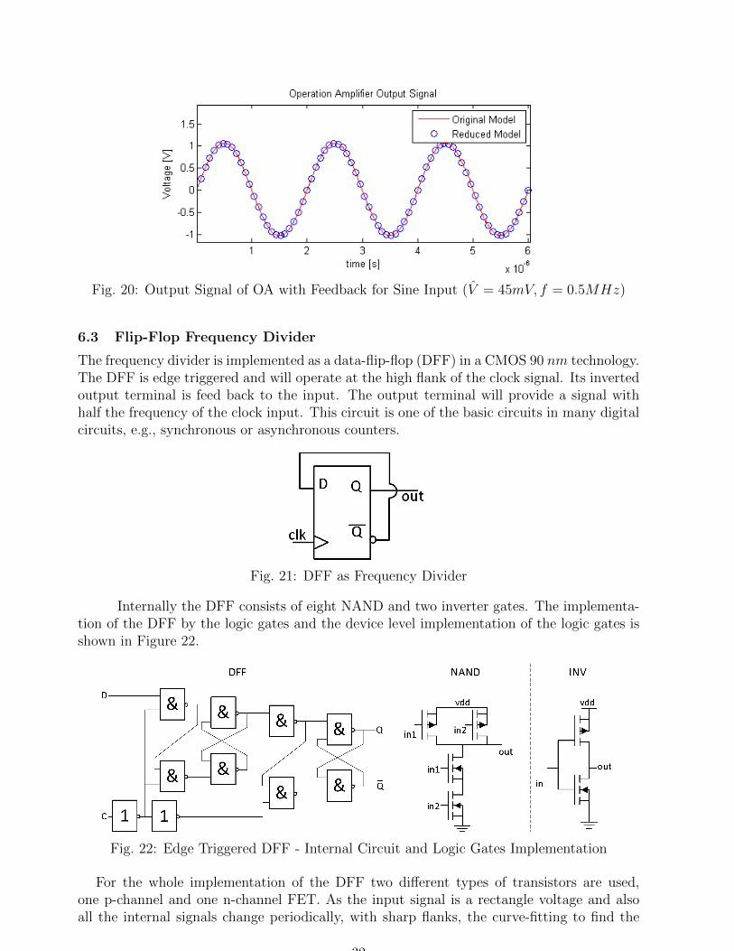
Fig. 20: Output Signal of OA with Feedback for Sine Input (V = 45mV, f = 0.5MHz)

6.3 Flip-Flop Frequency Divider

The frequency divider is implemented as a data-flip-flop (DFF) in a CMOS 90 nm technology.The DFF is edge triggered and will operate at the high flank of the clock signal. Its invertedoutput terminal is feed back to the input. The output terminal will provide a signal withhalf the frequency of the clock input. This circuit is one of the basic circuits in many digitalcircuits, e.g., synchronous or asynchronous counters.

Fig. 21: DFF as Frequency Divider

Internally the DFF consists of eight NAND and two inverter gates. The implementa-tion of the DFF by the logic gates and the device level implementation of the logic gates isshown in Figure 22.

Fig. 22: Edge Triggered DFF - Internal Circuit and Logic Gates Implementation

For the whole implementation of the DFF two different types of transistors are used,one p-channel and one n-channel FET. As the input signal is a rectangle voltage and alsoall the internal signals change periodically, with sharp flanks, the curve-fitting to find the

32

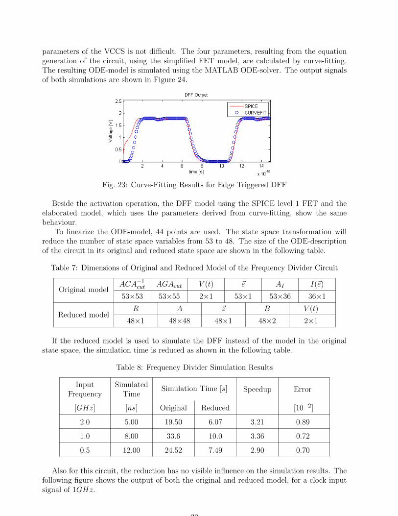
parameters of the VCCS is not difficult. The four parameters, resulting from the equationgeneration of the circuit, using the simplified FET model, are calculated by curve-fitting.The resulting ODE-model is simulated using the MATLAB ODE-solver. The output signalsof both simulations are shown in Figure 24.

Fig. 23: Curve-Fitting Results for Edge Triggered DFF

Beside the activation operation, the DFF model using the SPICE level 1 FET and theelaborated model, which uses the parameters derived from curve-fitting, show the samebehaviour.

To linearize the ODE-model, 44 points are used. The state space transformation willreduce the number of state space variables from 53 to 48. The size of the ODE-descriptionof the circuit in its original and reduced state space are shown in the following table.

Table 7: Dimensions of Original and Reduced Model of the Frequency Divider Circuit

Original modelACA−1

cut AGAcut V (t) ~e AI I(~e)

53×53 53×55 2×1 53×1 53×36 36×1

Reduced modelR A ~z B V (t)

48×1 48×48 48×1 48×2 2×1

If the reduced model is used to simulate the DFF instead of the model in the originalstate space, the simulation time is reduced as shown in the following table.

Table 8: Frequency Divider Simulation Results

InputFrequency

SimulatedTime

Simulation Time [s] Speedup Error

[GHz] [ns] Original Reduced [10−2]

2.0 5.00 19.50 6.07 3.21 0.89

1.0 8.00 33.6 10.0 3.36 0.72

0.5 12.00 24.52 7.49 2.90 0.70

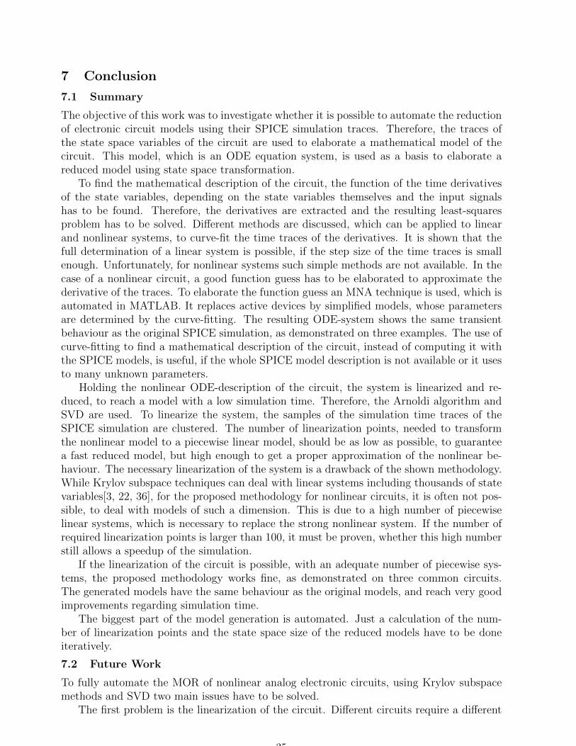
Also for this circuit, the reduction has no visible influence on the simulation results. Thefollowing figure shows the output of both the original and reduced model, for a clock inputsignal of 1GHz.

33

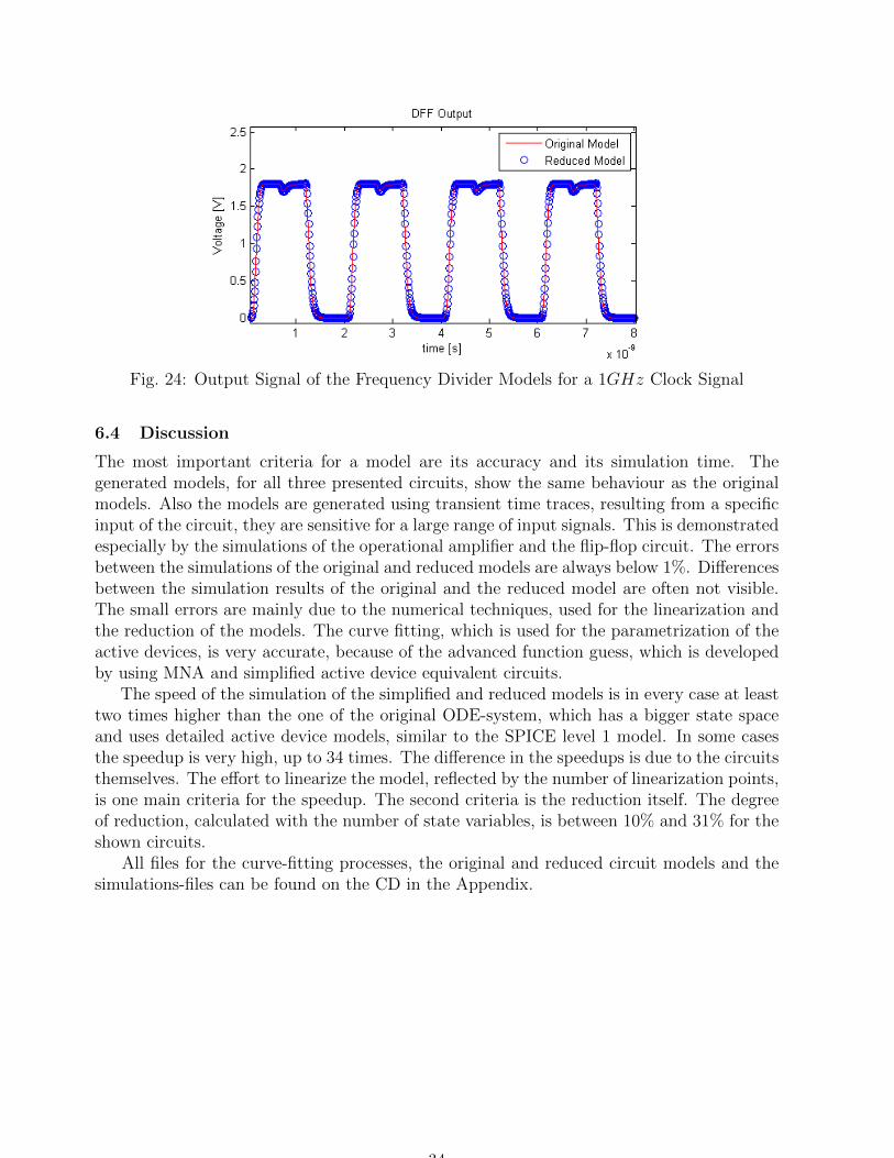
Fig. 24: Output Signal of the Frequency Divider Models for a 1GHz Clock Signal

6.4 Discussion

The most important criteria for a model are its accuracy and its simulation time. Thegenerated models, for all three presented circuits, show the same behaviour as the originalmodels. Also the models are generated using transient time traces, resulting from a specificinput of the circuit, they are sensitive for a large range of input signals. This is demonstratedespecially by the simulations of the operational amplifier and the flip-flop circuit. The errorsbetween the simulations of the original and reduced models are always below 1%. Differencesbetween the simulation results of the original and the reduced model are often not visible.The small errors are mainly due to the numerical techniques, used for the linearization andthe reduction of the models. The curve fitting, which is used for the parametrization of theactive devices, is very accurate, because of the advanced function guess, which is developedby using MNA and simplified active device equivalent circuits.

The speed of the simulation of the simplified and reduced models is in every case at leasttwo times higher than the one of the original ODE-system, which has a bigger state spaceand uses detailed active device models, similar to the SPICE level 1 model. In some casesthe speedup is very high, up to 34 times. The difference in the speedups is due to the circuitsthemselves. The effort to linearize the model, reflected by the number of linearization points,is one main criteria for the speedup. The second criteria is the reduction itself. The degreeof reduction, calculated with the number of state variables, is between 10% and 31% for theshown circuits.

All files for the curve-fitting processes, the original and reduced circuit models and thesimulations-files can be found on the CD in the Appendix.

34

7 Conclusion

7.1 Summary

The objective of this work was to investigate whether it is possible to automate the reductionof electronic circuit models using their SPICE simulation traces. Therefore, the traces ofthe state space variables of the circuit are used to elaborate a mathematical model of thecircuit. This model, which is an ODE equation system, is used as a basis to elaborate areduced model using state space transformation.

To find the mathematical description of the circuit, the function of the time derivativesof the state variables, depending on the state variables themselves and the input signalshas to be found. Therefore, the derivatives are extracted and the resulting least-squaresproblem has to be solved. Different methods are discussed, which can be applied to linearand nonlinear systems, to curve-fit the time traces of the derivatives. It is shown that thefull determination of a linear system is possible, if the step size of the time traces is smallenough. Unfortunately, for nonlinear systems such simple methods are not available. In thecase of a nonlinear circuit, a good function guess has to be elaborated to approximate thederivative of the traces. To elaborate the function guess an MNA technique is used, which isautomated in MATLAB. It replaces active devices by simplified models, whose parametersare determined by the curve-fitting. The resulting ODE-system shows the same transientbehaviour as the original SPICE simulation, as demonstrated on three examples. The use ofcurve-fitting to find a mathematical description of the circuit, instead of computing it withthe SPICE models, is useful, if the whole SPICE model description is not available or it usesto many unknown parameters.

Holding the nonlinear ODE-description of the circuit, the system is linearized and re-duced, to reach a model with a low simulation time. Therefore, the Arnoldi algorithm andSVD are used. To linearize the system, the samples of the simulation time traces of theSPICE simulation are clustered. The number of linearization points, needed to transformthe nonlinear model to a piecewise linear model, should be as low as possible, to guaranteea fast reduced model, but high enough to get a proper approximation of the nonlinear be-haviour. The necessary linearization of the system is a drawback of the shown methodology.While Krylov subspace techniques can deal with linear systems including thousands of statevariables[3, 22, 36], for the proposed methodology for nonlinear circuits, it is often not pos-sible, to deal with models of such a dimension. This is due to a high number of piecewiselinear systems, which is necessary to replace the strong nonlinear system. If the number ofrequired linearization points is larger than 100, it must be proven, whether this high numberstill allows a speedup of the simulation.

If the linearization of the circuit is possible, with an adequate number of piecewise sys-tems, the proposed methodology works fine, as demonstrated on three common circuits.The generated models have the same behaviour as the original models, and reach very goodimprovements regarding simulation time.

The biggest part of the model generation is automated. Just a calculation of the num-ber of linearization points and the state space size of the reduced models have to be doneiteratively.

7.2 Future Work

To fully automate the MOR of nonlinear analog electronic circuits, using Krylov subspacemethods and SVD two main issues have to be solved.

The first problem is the linearization of the circuit. Different circuits require a different

35

number linearization points. An analytical calculation of this number or at least an estima-tion of the number, based on the size of the circuit, its simulation traces and maybe the ratioof linear to nonlinear devices, is required essentially. Without the knowledge of the numberof piecewise systems a full automation is not possible.

The second weak point of the proposed methodology is the determination of the size ofthe subspace. This means that the Arnoldi algorithm has to be modified, to automaticallystop if a moment matching of the most important moments is finished. It would be a bigstep towards the automation of reduced systems, if such a break condition could be appliedsuccessfully.

To gain a faster speedup of the reduced models, the determination of the closest modelin each time step of the simulation has to be calculated faster. This can be done for exampleby limiting the systems taken into account, for the calculation of the closest linear system,by grouping them into subgroups, or using weight functions. This means, that not only theclosest linearization point, but maybe the closest two or three are used for the derivativecalculation. This technique should also reduce the number of necessary linearization points.

References

[1] R. Myslewski, “Moore’s law ’alive and well’,” The Register, 2013.

[2] P. Benner, H. M., and E. J. W. ter Maten, Model Reduction for Circuit Simulation.Springer, 2011.

[3] W. Schilders, H. van der Horst, and J. Rommes, Model Order Reduction: Theory,Research Aspects and Applications. Springer, 2008.

[4] M. Rewienski and J. White, “A Trajectory Piecewise-Linear Approach to Model OrderReduction and Fast Simulation of Nonlinear Circuits and Micromachined Devices,”Computer-Aided Design of Integrated Circuits and Systems, IEEE Transactions on,vol. 22, no. 2, pp. 155–170, 2003.

[5] H. Aridhi, M. H. Zaki, and S. Tahar, “Towards Improving Simulation of Analog CircuitsUsing Model Order Reduction,” IEEE/ACM Design Automation and Test in Europe,pp. 1337–1342, Mar 2012.

[6] N. Dongi and J. Roychowdhury, “General-Purpose Nonlinear Model-Order ReductionUsing Piecewise-Polynomial Representations,” IEEE Transactions on Computer AidedDesign of Integrated Circuits and Systems, vol. 27, no. 2, pp. 649 – 654, 2008.

[7] J. Phillips, L. Daniel, and L. Silveira, “Guaranteed Passive Balancing Transformationsfor Model Order Reduction,” IEEE Transactions on Computer-Aided Design of Inte-grated Circuits and Systems, vol. 22, no. 8, pp. 1027–1041, 2003.

[8] P. Heydari and M. Pedram, “Model-Order Reduction Using Variational Balanced Trun-cation with Spectral Shaping,” IEEE Transactions on Circuits and Systems I: RegularPapers, vol. 53, no. 4, pp. 879–891, 2006.

[9] R. Prasad, “Pade Type Model Order Reduction for Multivariable Systems Using RouthApproximation,” Computers and Electrical Engineering, vol. 26, no. 6, pp. 445 – 459,2000.

[10] Y. C. L. et al., “Proper Orthogonal Decomposition and its Applications,” Journal ofSound and Vibration, 2002.

36

[11] M. Ahmadloo and A. Dounavis, “Parameterized Model Order Reduction of Electromag-netic Systems Using Multiorder Arnoldi,” IEEE Transactions on Advanced Packaging,vol. 33, no. 4, pp. 1012–1020, 2010.

[12] R. W. Freund, “Krylov-Subspace Methods for Reduced-Order Modeling in Circuit Sim-ulation,” Journal of Computational and Applied Mathematics, vol. 123, no. 1-2, pp. 395– 421, 2000.

[13] A. Steinbrecher and T. Stykel, “Model Order Reduction of Electrical Circuits with Non-linear Elements,” in Progress in Industrial Mathematics at ECMI 2010 (M. Gunther,A. Bartel, M. Brunk, S. Schops, and M. Striebel, eds.), Mathematics in Industry,pp. 169–177, Springer, 2012.

[14] I. Aris, L. Hulley, N. Mariun, and R. Sahbudin, “Using Curve-Fitting OptimisationTechnique to Estimate Power MOSFET Model Parameters for PECT II System,” in1998. Proceedings. ICSE ’98. 1998 IEEE International Conference on SemiconductorElectronics, pp. 157–161, 1998.

[15] SPICE Model Generator. Agilent Technologies, 395 Page Mill Road, Palo Alto, CA94304 USA, 2013.

[16] R. Duraiswami, “Computational Methods, Lecture Notes,” tech. rep., Univer-sity of Maryland, Jan 2013. http : //www.umiacs.umd.edu/ ramani/cmsc460/Lecture1 Introduction 2013.pdf .

[17] L. Nagel, SPICE2: A Computer Program to Simulate Semiconductor Circuits. Mem-orandum, Electronics Research Laboratory, College of Engineering, University of Cali-fornia, USA, 1975.

[18] T. Tuma and A. Burmen, Circuit Simulation with SPICE OPUS: Theory and Practice.Birkhauser, 1st ed., 2009.

[19] Avant! Star-Hspice Manual. 46871 Bayside Parkway Fremont, CA 94538, 1998.

[20] C. Desoer and E. Kuh, Basic Circuit Theory. McGraw-Hill Education (India), 2009.

[21] F. N. Najm, Circuit Simulation. Wiley, 2010.

[22] T. Reis and T. Stykel, “Modellreduktion von RC Schaltungen,” tech. rep., ElgersburgWorkshop Mathematische Systemtheorie, Elgersburg, 2013.

[23] C. Hymowitz, “Step-by-Step Procedures Help you Solve Spice Convergence Problems,”EDN, 1994.

[24] L. Trefethen and D. Bau, Numerical Linear Algebra. Society for Industrial and AppliedMathematics, 1997.

[25] M.-H. Lai, C.-C. Chu, and W.-S. Feng, “MIMO Interconnects Order Reductions byUsing the Global Arnoldi Algorithm,” in IEEE International Symposium on Circuitsand Systems, pp. 4 pp.–1110, 2006.

[26] Z. Yacine, A. Benfdila, and S. Djennoune, “Model Order Reduction of Nonlinear Sys-tems via the Trajectory Piecewise Linear Approach Application to Transmission LinesCircuit,” in New aspects of applied informatics and communications Part II, pp. 369–375, 1998.

37

[27] A. C. Antoulas and D. C. Sorensen, “Approximation of Large-Scale Dynamical Systems:An Overview,” Applied Mathematics and Computer Science, vol. 11, no. 5, pp. 1093–1122, 2001.

[28] P. Sen and G. I. of Technology, Estimation and Optimization of Layout Parasitics forSilicon-based Millimeter-Wave Integrated Circuits. Georgia Institute of Technology,2007.

[29] D. W. Harder, “Numerical Analysis, 5.1 Vandermonde,” tech. rep., University of Wa-terloo, 2013.

[30] E. W. Weisstein, “Vandermonde Matrix,” tech. rep., MathWorld, 2013.http://mathworld.wolfram.com/VandermondeMatrix.html.

[31] H. Gavin, “The Levenberg-Marquardt Method for Nonlinear Least Squares Curve-Fitting Problems,” Sept. 2013.

[32] M. K. Transtrum and J. P. Sethna, “Improvements to the Levenberg-Marquardt Al-gorithm for Nonlinear Least-Squares Minimization,” arXiv preprint arXiv:1201.5885,2012.

[33] D. W. Marquardt, “An Algorithm for Least-Squares Estimation of Nonlinear Param-eters,” Journal of the Society for Industrial & Applied Mathematics, vol. 11, no. 2,pp. 431–441, 1963.

[34] E. W. Weisstein, K-Means Clustering Algorithm. MathWorld-A Wolfram Web Resource,http://mathworld.wolfram.com/K-MeansClusteringAlgorithm.html, 2013.

[35] J. DErrico, “Adaptive Robust Numerical Differentiation,” tech. rep., MATLAB Central,2013.

[36] P. Miettinen, M. Honkala, J. Roos, and M. Valtonen, “PartMOR: Partitioning-BasedRealizable Model-Order Reduction Method for RLC Circuits,” IEEE Transactions onComputer-Aided Design of Integrated Circuits and Systems, vol. 30, no. 3, pp. 374–387,2011.

38