Model Selection and Bootstrapping

� So you’ve made a model

� What’s Next? ◦ How to choose the appropriate model for your

data? ◦ Which Criteria should you use? ◦ Avoiding the overfit

Model Selection

Model Selection Techniques � Akaike Information Criteria

� Bayesian Information Criteria

� Mallow’s Cp

� Stepwise Regression

� Cross validation

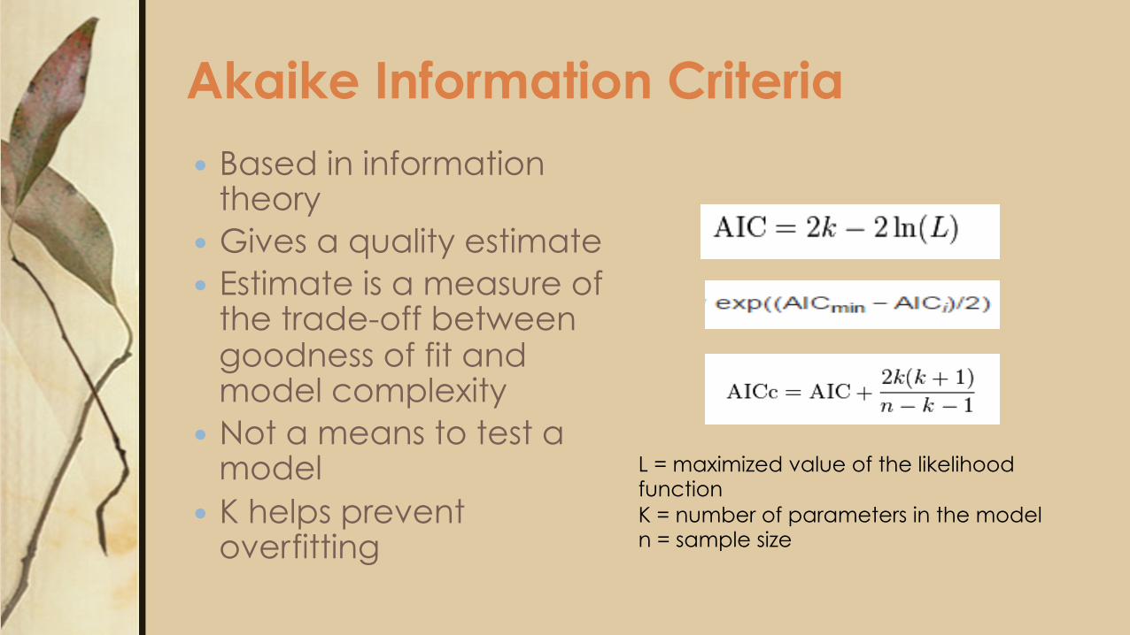
Akaike Information Criteria �  Based in information

theory �  Gives a quality estimate �  Estimate is a measure of

the trade-off between goodness of fit and model complexity

�  Not a means to test a model

�  K helps prevent overfitting

L = maximized value of the likelihood function K = number of parameters in the model n = sample size

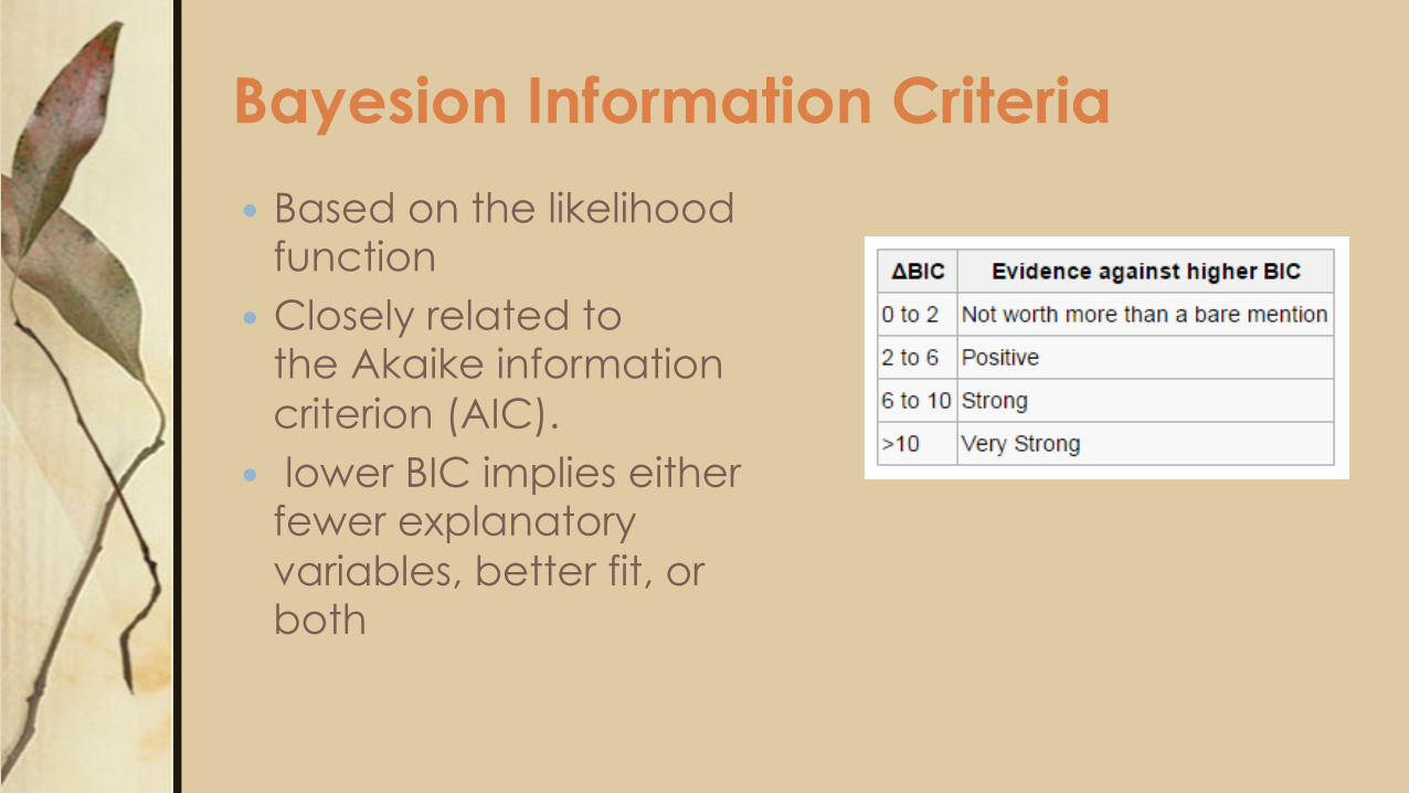
Bayesion Information Criteria

�  Based on the likelihood function 

�  Closely related to the Akaike information criterion (AIC).

�   lower BIC implies either fewer explanatory variables, better fit, or both

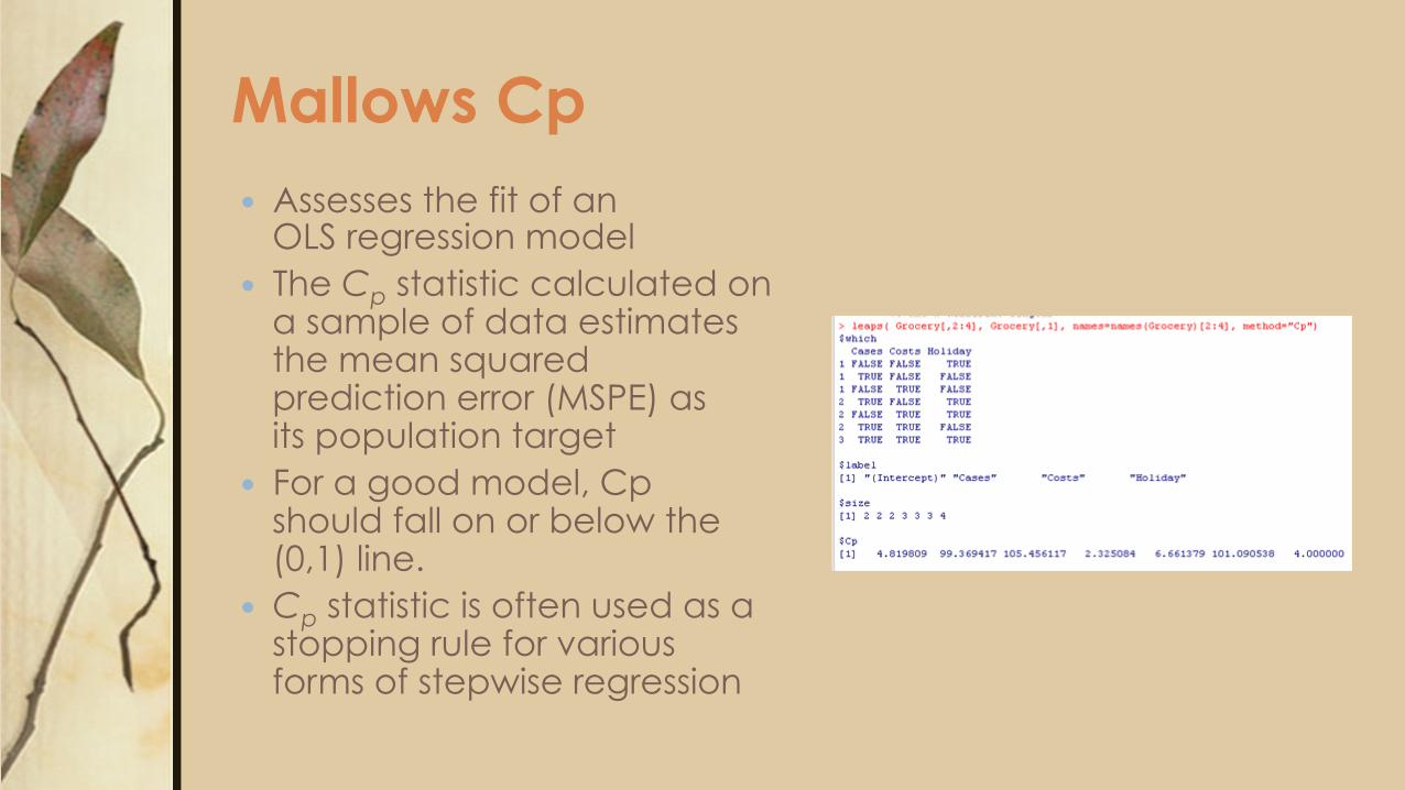
Mallows Cp �  Assesses the fit of an

OLS regression model  �  The Cp statistic calculated on

a sample of data estimates the mean squared prediction error (MSPE) as its population target

�  For a good model, Cp should fall on or below the (0,1) line.

�  Cp statistic is often used as a stopping rule for various forms of stepwise regression

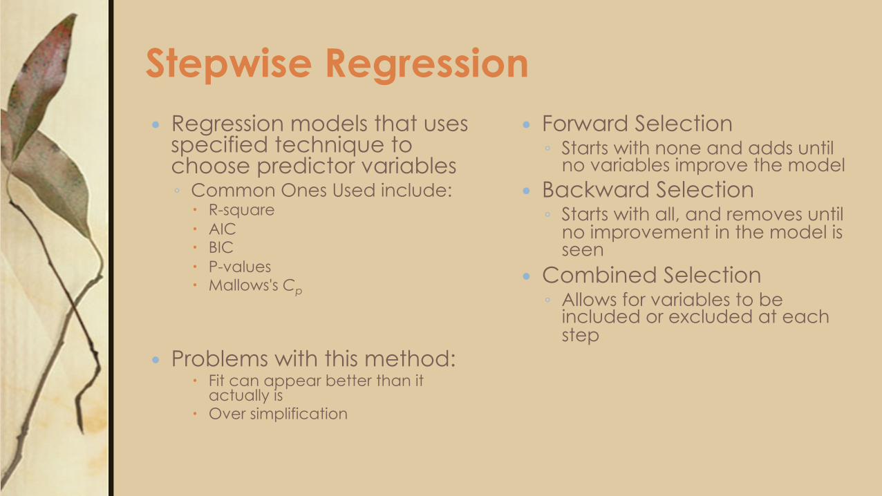
Stepwise Regression �  Regression models that uses

specified technique to choose predictor variables ◦  Common Ones Used include:

�  R-square �  AIC �  BIC �  P-values �  Mallows's Cp

�  Problems with this method: �  Fit can appear better than it

actually is �  Over simplification

�  Forward Selection ◦  Starts with none and adds until

no variables improve the model �  Backward Selection ◦  Starts with all, and removes until

no improvement in the model is seen

�  Combined Selection ◦  Allows for variables to be

included or excluded at each step

Cross Validation

�  Assesses how the results of a statistical analysis will fit to an independent data set

�  Start with a training data to develop model

�  Model is tested using test data �  Can subset original data into training

and test data �  Useful for data that is difficult or costly

to collect

Bootstrapping

Get to Liftin’

Traditional inference �  From any sample, we can figure only one of each

statistic (e.g. mean, var, F, AIC, etc.) � What we don’t know is information on the

distribution of that statistic (e.g., shape, variance, skewness, etc.)

�  traditional inference infers the distribution of a statistic given that certain assumptions are met; typically: Ø Independence of residuals Ø  Normality of residuals Ø  Equality of variance of residuals

Limitations to traditional inference �  p-values and confidence intervals are suspect when

assumptions are violated �  The sampling distribution of a statistic is often unknown and

prohibitively difficult to derive

�  Seeks to find the distribution of any possible statistic or function ◦  without assumptions about the population distribution ◦  without deriving the sampling distribution explicitly ◦  only from knowledge of the sample itself; i.e., the sample

pulls itself up by its bootstraps

The bootstrap…

Bootstrapping is a method for estimating the sampling distribution of an estimator by resampling with replacement from the original sample.

�  means of estimating the statistical accuracy from the data in a single sample.

�  Mimics the process of selecting many samples when the population is

too small to do otherwise �  The samples are generated from the data in the original sample by

copying it many number of times (Monte Carlo Simulation) �  Samples can then be selected at random and descriptive statistics

calculated or regressions run for each sample �  The results generated from the bootstrap samples can be treated as if

it they were the result of actual sampling from the original population

The Idea: Try to do what can’t do in real life – take lots and lots of independent samples. �  Perform desired function on multiple*subsamples* ◦  Subsamples: same size as original sample, but chosen *with

replacement* �  With Replacement: if a number has already been picked to

be in the subsample, it is still eligible to be picked a second time, third time, etc. This is called resampling your data.

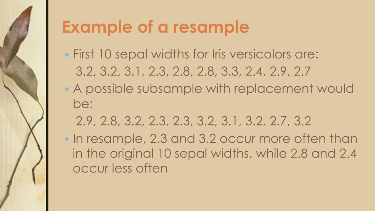
Example of a resample

� First 10 sepal widths for Iris versicolors are: 3.2, 3.2, 3.1, 2.3, 2.8, 2.8, 3.3, 2.4, 2.9, 2.7 � A possible subsample with replacement would

be: 2.9, 2.8, 3.2, 2.3, 2.3, 3.2, 3.1, 3.2, 2.7, 3.2 �  In resample, 2.3 and 3.2 occur more often than

in the original 10 sepal widths, while 2.8 and 2.4 occur less often

Results – bootstrapped confidence interval

�  The distribution of the resample results are centered around the results of the original sample.

�  To test for significance, form a 100(1-α)% confidence interval then check to see if that interval contains 0.

Virtually assumption free, except…

�  That the distribution of your sample is a close approximation to the population distribution. ◦  Tends to be true as # samples (n) becomes large ◦  But if n is small, this is precisely when violations of assumptions for

traditional statistics matters most ◦  The bootstrap has been criticized on these grounds: it can’t help

us precisely when we need it most! ◦  Inference will always be suspect for small samples. However, it

allows us to estimate heretofore unknowable sampling distributions.

Ecological Applications �  Ecologists often use cluster analysis as a tool in the classification

and mapping of entities such as communities or landscapes �  However, the researcher has to choose an adequate group

partition level �  Use bootstrap to test statistically for fuzziness of the partitions in

cluster analysis �  Partitions found in bootstrap samples are compared to the

observed partition by the similarity of the sampling units that form the groups.

Example: Iris data – is there a difference in mean sepal widths between the Iris versicolor and I. virginica?

� Using first 10 samples from each species � Difference in mean sepal widths is -0.07. Is this large

or small?? Ho: There is no difference in mean sepal width between these two species Ha: There is a difference in mean sepal width between these two species

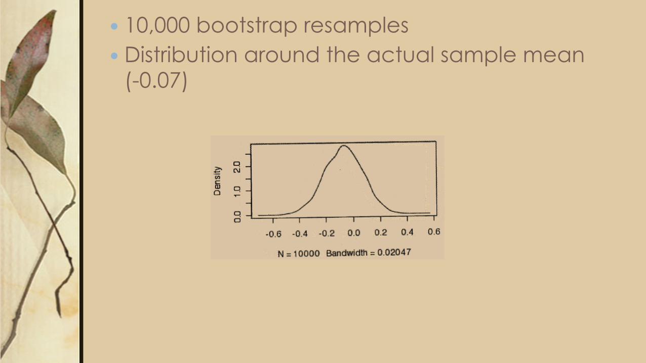
� 10,000 bootstrap resamples � Distribution around the actual sample mean

(-0.07)

� A 95% confidence interval for the population mean difference can be found by taking the middle 9,500 mean differences from the 10,000 in our bootstrap distribution

�  This results in an interval of (-0.36, 0.20) � A population mean difference of 0 is plausible,

and there is not significant evidence to reject the null hypothesis (no difference in sepal length)