Embed Size (px)
Citation preview
Modeling and Analysis of Dynamic Systems
by Dr. Guillaume Ducard c©
Fall 2017
Institute for Dynamic Systems and Control
ETH Zurich, Switzerland
G. Ducard c© 1 / 33
Outline
1 Introduction
2 System Modeling for Control
G. Ducard c© 2 / 33
IntroductionSystem Modeling for Control
Definitions: Modeling and Analysis of Dynamic Systems
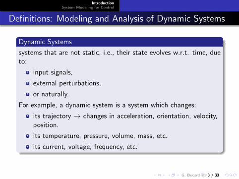
Dynamic Systems
systems that are not static, i.e., their state evolves w.r.t. time, dueto:
input signals,
external perturbations,
or naturally.
For example, a dynamic system is a system which changes:
its trajectory → changes in acceleration, orientation, velocity,position.
its temperature, pressure, volume, mass, etc.
its current, voltage, frequency, etc.
G. Ducard c© 3 / 33
IntroductionSystem Modeling for Control
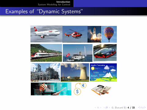
Examples of “Dynamic Systems”
G. Ducard c© 4 / 33
IntroductionSystem Modeling for Control
Definition: “Modeling and Analysis”
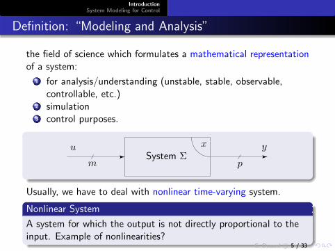
the field of science which formulates a mathematical representationof a system:
1 for analysis/understanding (unstable, stable, observable,controllable, etc.)
2 simulation3 control purposes.
u
mSystem Σ
x
p
y
Usually, we have to deal with nonlinear time-varying system.
Nonlinear System
A system for which the output is not directly proportional to theinput. Example of nonlinearities?
G. Ducard c© 5 / 33
IntroductionSystem Modeling for Control
Definition: “Modeling and Analysis”
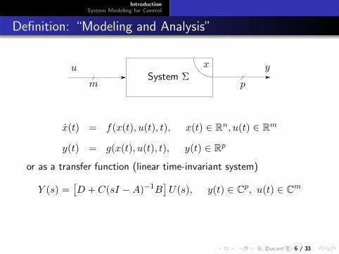
u
mSystem Σ
x
p
y
x(t) = f(x(t), u(t), t), x(t) ∈ Rn, u(t) ∈ R
m
y(t) = g(x(t), u(t), t), y(t) ∈ Rp
or as a transfer function (linear time-invariant system)
Y (s) =[
D + C(sI −A)−1B]
U(s), y(t) ∈ Cp, u(t) ∈ C
m
G. Ducard c© 6 / 33
IntroductionSystem Modeling for Control
Model Synthesis
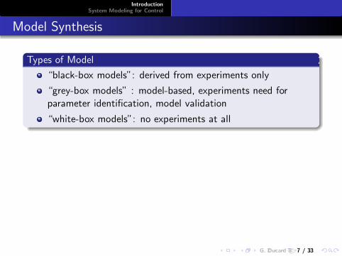
Types of Model
“black-box models”: derived from experiments only
“grey-box models” : model-based, experiments need forparameter identification, model validation
“white-box models”: no experiments at all
G. Ducard c© 7 / 33
IntroductionSystem Modeling for Control
Model Synthesis
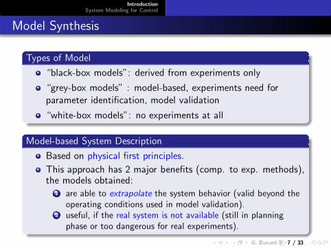
Types of Model
“black-box models”: derived from experiments only
“grey-box models” : model-based, experiments need forparameter identification, model validation
“white-box models”: no experiments at all
Model-based System Description
Based on physical first principles.
This approach has 2 major benefits (comp. to exp. methods),the models obtained:
1 are able to extrapolate the system behavior (valid beyond theoperating conditions used in model validation).
2 useful, if the real system is not available (still in planningphase or too dangerous for real experiments).
G. Ducard c© 7 / 33
IntroductionSystem Modeling for Control
Why Use Models?
1 System analysis and synthesis
2 Feedforward control systems
3 Feedback control systems
G. Ducard c© 8 / 33
IntroductionSystem Modeling for Control
Why Use Models?
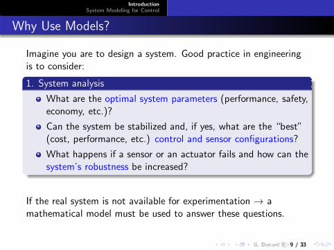
Imagine you are to design a system. Good practice in engineeringis to consider:
1. System analysis
What are the optimal system parameters (performance, safety,economy, etc.)?
Can the system be stabilized and, if yes, what are the “best”(cost, performance, etc.) control and sensor configurations?
What happens if a sensor or an actuator fails and how can thesystem’s robustness be increased?
If the real system is not available for experimentation → amathematical model must be used to answer these questions.
G. Ducard c© 9 / 33
IntroductionSystem Modeling for Control
Why Use Models?
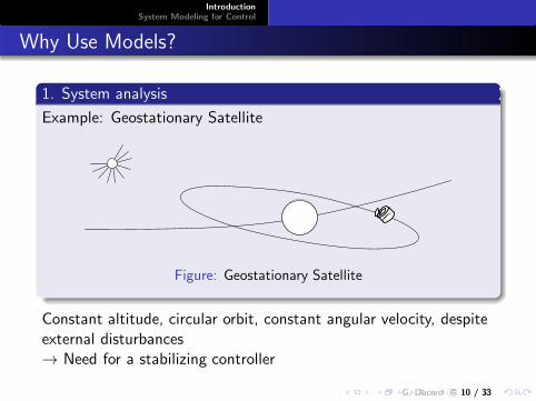
1. System analysis
Example: Geostationary Satellite
Figure: Geostationary Satellite
Constant altitude, circular orbit, constant angular velocity, despiteexternal disturbances→ Need for a stabilizing controller
G. Ducard c© 10 / 33
IntroductionSystem Modeling for Control
Why Use Models?
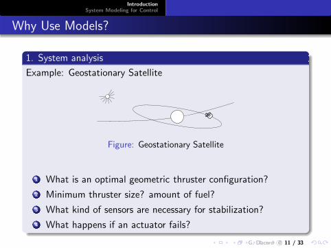
1. System analysis
Example: Geostationary Satellite
Figure: Geostationary Satellite
1 What is an optimal geometric thruster configuration?
2 Minimum thruster size? amount of fuel?
3 What kind of sensors are necessary for stabilization?
4 What happens if an actuator fails?
G. Ducard c© 11 / 33
IntroductionSystem Modeling for Control
Why Use Models?
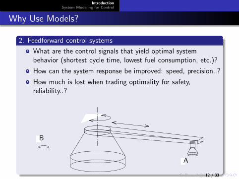
2. Feedforward control systems
What are the control signals that yield optimal systembehavior (shortest cycle time, lowest fuel consumption, etc.)?
How can the system response be improved: speed, precision..?
How much is lost when trading optimality for safety,reliability..?
A
B
G. Ducard c© 12 / 33
IntroductionSystem Modeling for Control
Why Use Models?
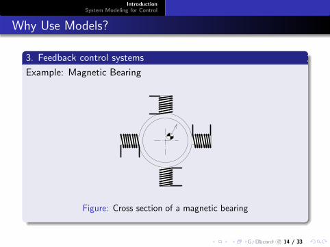
3. Feedback control systems
How can system stability be maintained for a given set ofexpected modeling errors?
How can a specified disturbance rejection (robustness) beguaranteed for disturbances acting in specific frequencybands?
What are the minimum and maximum bandwidths that acontroller must attain for a specific system in order forstability and performance requirements to be guaranteed?
G. Ducard c© 13 / 33
IntroductionSystem Modeling for Control
Why Use Models?
3. Feedback control systems
Example: Magnetic Bearing
Figure: Cross section of a magnetic bearing
G. Ducard c© 14 / 33
IntroductionSystem Modeling for Control
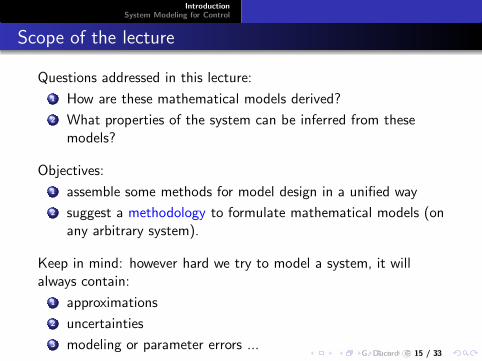
Scope of the lecture
Questions addressed in this lecture:
1 How are these mathematical models derived?
2 What properties of the system can be inferred from thesemodels?
Objectives:
1 assemble some methods for model design in a unified way
2 suggest a methodology to formulate mathematical models (onany arbitrary system).
Keep in mind: however hard we try to model a system, it willalways contain:
1 approximations
2 uncertainties
3 modeling or parameter errors ...G. Ducard c© 15 / 33
IntroductionSystem Modeling for Control
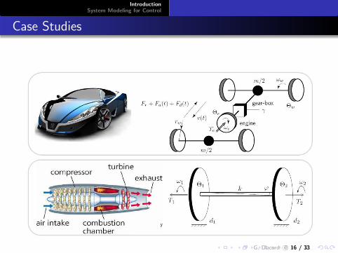
Case Studies
G. Ducard c© 16 / 33
IntroductionSystem Modeling for Control
Case Studies
G. Ducard c© 17 / 33
IntroductionSystem Modeling for Control
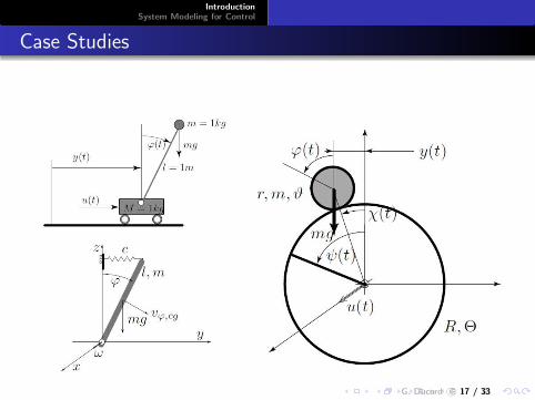
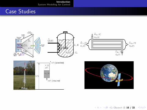
Case Studies
G. Ducard c© 18 / 33
IntroductionSystem Modeling for Control
2. System Modeling for Control
G. Ducard c© 19 / 33
IntroductionSystem Modeling for Control
Types of Modeling: Definitions
u
mSystem Σ
x
p
y
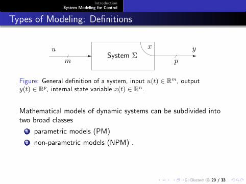
Figure: General definition of a system, input u(t) ∈ Rm, outputy(t) ∈ Rp, internal state variable x(t) ∈ Rn.
Mathematical models of dynamic systems can be subdivided intotwo broad classes
1 parametric models (PM)
2 non-parametric models (NPM) .
G. Ducard c© 20 / 33
IntroductionSystem Modeling for Control
Types of Modeling: Definitions
u
mSystem Σ
x
p
y
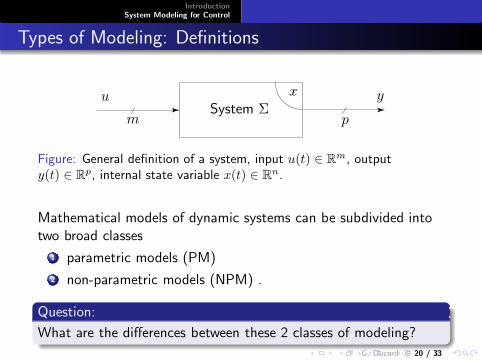
Figure: General definition of a system, input u(t) ∈ Rm, outputy(t) ∈ Rp, internal state variable x(t) ∈ Rn.
Mathematical models of dynamic systems can be subdivided intotwo broad classes
1 parametric models (PM)
2 non-parametric models (NPM) .
Question:
What are the differences between these 2 classes of modeling?
G. Ducard c© 20 / 33
IntroductionSystem Modeling for Control
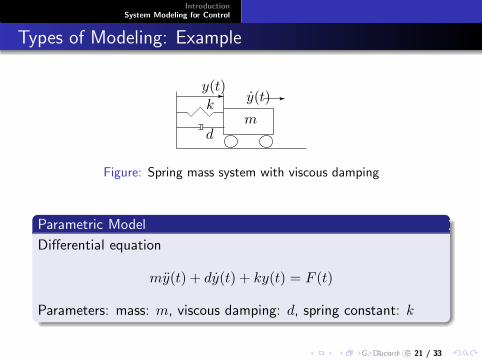
Types of Modeling: Example
y(t)
k
dm
y(t)
Figure: Spring mass system with viscous damping
Parametric Model
Differential equation
my(t) + dy(t) + ky(t) = F (t)
Parameters: mass: m, viscous damping: d, spring constant: k
G. Ducard c© 21 / 33
IntroductionSystem Modeling for Control
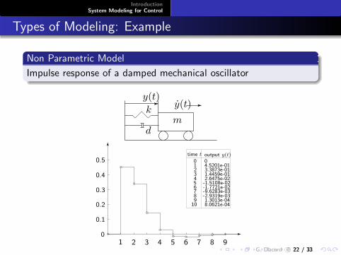
Types of Modeling: Example
Non Parametric Model
Impulse response of a damped mechanical oscillatorPSfrag
y(t)
k
dm
y(t)
time t output y(t)
0
0.1
0.2
0.3
0.4
0.5
1 2 3 4 5 6 7 8 9
012345678910
04.5201e-013.3873e-011.4459e-012.6475e-02-1.5108e-02-1.7721e-02-9.6283e-03-2.9319e-031.3013e-048.0621e-04
G. Ducard c© 22 / 33
IntroductionSystem Modeling for Control
Types of Modeling: Discussion
Non parametric models have several drawbacks
1 they require the system to be accessible for experiments
2 they cannot predict the behavior of the system if modified
3 not useful for systematic design optimization
During this lecture, we will only consider parametric modeling.
G. Ducard c© 23 / 33
IntroductionSystem Modeling for Control
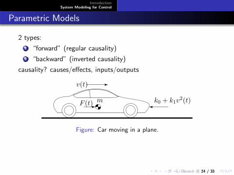
Parametric Models
2 types:
1 “forward” (regular causality)
2 “backward” (inverted causality)
causality? causes/effects, inputs/outputs
v(t)
F (t) m k0 + k1v2(t)
Figure: Car moving in a plane.
G. Ducard c© 24 / 33
IntroductionSystem Modeling for Control
Parametric Models
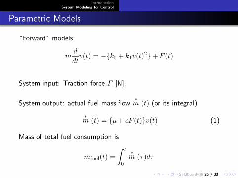
“Forward” models
md
dtv(t) = −{k0 + k1v(t)
2}+ F (t)
System input: Traction force F [N].
System output: actual fuel mass flow∗
m (t) (or its integral)
∗
m (t) = {µ+ ǫF (t)}v(t) (1)
Mass of total fuel consumption is
mfuel(t) =
∫ t
0
∗
m (τ)dτ
G. Ducard c© 25 / 33
IntroductionSystem Modeling for Control
Parametric Models
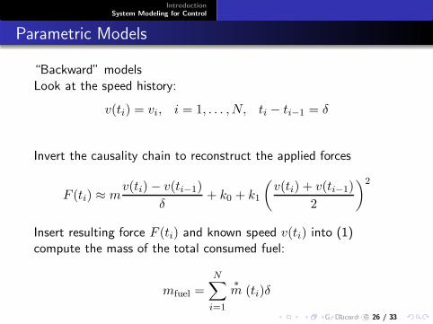
“Backward” modelsLook at the speed history:
v(ti) = vi, i = 1, . . . , N, ti − ti−1 = δ
Invert the causality chain to reconstruct the applied forces
F (ti) ≈ mv(ti)− v(ti−1)
δ+ k0 + k1
(
v(ti) + v(ti−1)
2
)2
Insert resulting force F (ti) and known speed v(ti) into (1)compute the mass of the total consumed fuel:
mfuel =
N∑
i=1
∗
m (ti)δ
G. Ducard c© 26 / 33
IntroductionSystem Modeling for Control
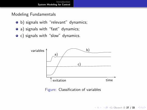
Modeling Fundamentals
b) signals with “relevant” dynamics;
a) signals with “fast” dynamics;
c) signals with “slow” dynamics.
variablesa)
b)
c)
exitation time
Figure: Classification of variables
G. Ducard c© 27 / 33
IntroductionSystem Modeling for Control
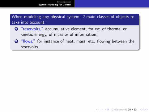
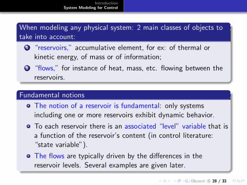
When modeling any physical system: 2 main classes of objects totake into account:
1 “reservoirs,” accumulative element, for ex: of thermal orkinetic energy, of mass or of information;
2 “flows,” for instance of heat, mass, etc. flowing between thereservoirs.
G. Ducard c© 28 / 33
IntroductionSystem Modeling for Control
When modeling any physical system: 2 main classes of objects totake into account:
1 “reservoirs,” accumulative element, for ex: of thermal orkinetic energy, of mass or of information;
2 “flows,” for instance of heat, mass, etc. flowing between thereservoirs.
Fundamental notions
The notion of a reservoir is fundamental: only systemsincluding one or more reservoirs exhibit dynamic behavior.
To each reservoir there is an associated “level” variable that isa function of the reservoir’s content (in control literature:“state variable”).
The flows are typically driven by the differences in thereservoir levels. Several examples are given later.
G. Ducard c© 28 / 33
IntroductionSystem Modeling for Control
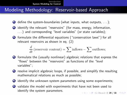
Modeling Methodology: Reservoir-based Approach
1 define the system-boundaries (what inputs, what outputs, . . . );
2 identify the relevant “reservoirs” (for mass, energy, information,. . . ) and corresponding “level variables” (or state variables);
3 formulate the differential equations (“conservation laws”) for allrelevant reservoirs as shown in eq. (2)
d
dt(reservoir content) =
∑
inflows−∑
outflows;
4 formulate the (usually nonlinear) algebraic relations that express the“flows” between the “reservoirs” as functions of the “levelvariables”;
5 resolve implicit algebraic loops, if possible, and simplify the resultingmathematical relations as much as possible;
6 identify the unknown system parameters using some experiments;
7 validate the model with experiments that have not been used toidentify the system parameters.
G. Ducard c© 29 / 33
IntroductionSystem Modeling for Control
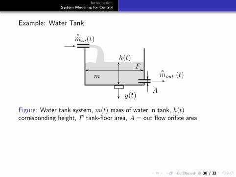
Example: Water Tank
∗
min(t)
∗
mout (t)F
Ay(t)
h(t)
m
Figure: Water tank system, m(t) mass of water in tank, h(t)corresponding height, F tank-floor area, A = out flow orifice area
G. Ducard c© 30 / 33
IntroductionSystem Modeling for Control
Modeling the water tank
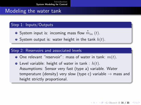
Step 1: Inputs/Outputs
System input is: incoming mass flow∗
min (t).
System output is: water height in the tank h(t).
G. Ducard c© 31 / 33
IntroductionSystem Modeling for Control
Modeling the water tank
Step 1: Inputs/Outputs
System input is: incoming mass flow∗
min (t).
System output is: water height in the tank h(t).
Step 2: Reservoirs and associated levels
One relevant “reservoir”: mass of water in tank: m(t).
Level variable: height of water in tank : h(t).Assumptions: Sensor very fast (type a) variable. Watertemperature (density) very slow (type c) variable → mass andheight strictly proportional.
G. Ducard c© 31 / 33
IntroductionSystem Modeling for Control
Modeling the water tank
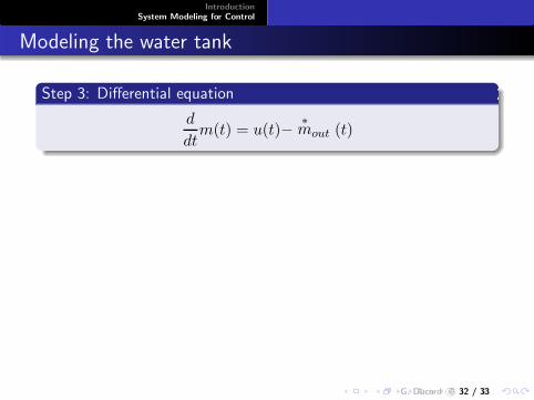
Step 3: Differential equation
d
dtm(t) = u(t)−
∗
mout (t)
G. Ducard c© 32 / 33
IntroductionSystem Modeling for Control
Modeling the water tank
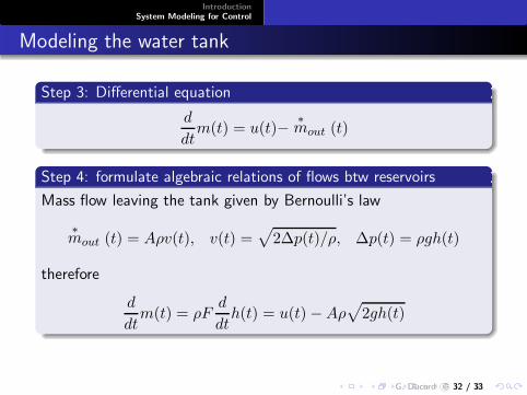
Step 3: Differential equation
d
dtm(t) = u(t)−
∗
mout (t)
Step 4: formulate algebraic relations of flows btw reservoirs
Mass flow leaving the tank given by Bernoulli’s law
∗
mout (t) = Aρv(t), v(t) =√
2∆p(t)/ρ, ∆p(t) = ρgh(t)
therefore
d
dtm(t) = ρF
d
dth(t) = u(t)−Aρ
√
2gh(t)
G. Ducard c© 32 / 33

IntroductionSystem Modeling for Control
Modeling the water tank
Causality Diagramsreplacements
∗
min(t) = u(t)
∗
mout (t)
mass reservoir
orifice
y(t)h(t)
-
+
Figure: Causality diagram of the water tank system, shaded blocksrepresent dynamical subsystems (containing reservoirs), plain blocksrepresent static subsystems.
G. Ducard c© 33 / 33