MODELING AND ANALYSIS OF TWO ALTERNATIVES FOR …

Carlos Eduardo Silva de Souza

MODELING AND ANALYSIS OF TWO

ALTERNATIVES FOR UNDERWAY SHIP-TO-

SHIP TRANSFER OF OIL IN OPEN SEA

São Paulo – 2012

Carlos Eduardo Silva de Souza

MODELING AND ANALYSIS OF TWO

ALTERNATIVES FOR UNDERWAY SHIP-TO-

SHIP TRANSFER OF OIL IN OPEN SEA

Dissertation presented to Escola

Politécnica da Universidade de São Paulo

for achievement of the degree of Master of

Science in Engineering.

Area of concentration: Naval Architecture

and Ocean Engineering

Supervisor: Prof. Dr. Helio Mitio

Morishita

São Paulo – 2012

This work is dedicated in memoriam

to my grandfather, vô Zé.

ACKNOWLEDGEMENTS

I am sincerely grateful to my supervisor, Prof. Dr. Helio Mitio Morishita, for the

long discussions throughout my Master’s and the opportunity of working in his

research group since the 3rd year of my Bachelor’s course.

Also fundamental for the development of this work were the support of Prof. Dr.

Alexandre Nicolaos Simos and Prof. Dr. Eduardo Aoun Tannuri, who provided

me valuable light in specific topics of my research.

Other specialists outside USP are acknowledged for have kindly shared their

experience on different topics of this work. They are Prof. Dr. Alexandros Glykas

(NTUA, Greece), Prof. Dr. Hiroyuki Oda (TUMSAT, Japan), Prof. Dr. Thor

Fossen and Dr. Xu Xiang (NTNU, Norway) and Prof. Dr. Tristan Perez (Univ. of

Newcastle, Australia).

My routine in the university allowed me to grow friendships that by no means

could be disregarded in this space. Thank you Anderson, João, Kevin, Massa,

Montanha, Sophie and Yuba for the fellowship and moments of amusement.

Besides, I could never fail to express how privileged I have been along this

journey to have people like Caio, 16, Eduardo, Itajubá, Larissa, Lázaro, Lu, Luís,

Natália, Pará, Rafael and Rubens as friends. Thank you, guys, for the stimulus,

the companionship, the comfort, the discussions, the jazz, the chess, the

tapiocas, the soccer and the beers.

Two people deserve my highest considerations, for they certainly are the most

responsible for the accomplishment of this work. I fondly thank my parents,

Elisa and Gilson, for so many years of patience, support and renunciations in

behalf of my education and growing. I also thank to my sister, Lívia, for teaching

me that life is not to be taken seriously. And to the rest of my (big) family,

specially my grandparents, for the indispensable incentives along all of my life.

And thank you, God, for having blessed me with this family and for giving me

strength to face my daily challenges.

Finally, I would like to manifest genuine gratitude to Transpetro, for supporting

this research. And to CAPES, for the granted scholarship.

ABSTRACT

Shuttle tankers with dynamic positioning (DP) systems are expensive ships.

Therefore, it is desirable to optimize their usage by, e.g., eliminating the travels

between offshore platforms and the terminals in the coast. When the oil is

intended to exportation, an attractive idea is to transfer it between the shuttle

tanker and the exporter ship (usually a VLCC) in open sea, close to the oil fields.

However, since a VLCC is rarely provided with a DP system, it is necessary to

develop alternative ways of attaining controllability of both vessels while the

transfer operation is performed. In this sense, two configurations for the so-

called ship-to-ship operations are proposed. One of them consists in performing

the transfer with underway ships, arranged side-by-side. The vessels are moored

together and the VLCC develops power ahead, towing the idle shuttle tanker.

Another alternative is to transfer the oil while the ships maintain a convoy

formation, with the VLCC trailing a given trajectory and being followed by the

shuttle tanker, which keeps a constant relative position by means of an

appropriate autopilot strategy. Dynamic models are developed for both

operations and implemented in numerical simulators. The simulations results

are discussed and used to outline the operational viability under different

combinations of environment and loading conditions.

TABLE OF CONTENTS

LIST OF FIGURES

LIST OF TABLES

LIST OF SYMBOLS

1. INTRODUCTION ...................................................................................... 22

1.1 OPERATIONS DESCRIPTION ............................................................... 25

1.1.1 Side-by-side...................................................................................... 25

1.1.2 Convoy .............................................................................................. 27

1.2 LITERATURE REVIEW ......................................................................... 28

1.3 OBJECTIVES .......................................................................................... 31

1.4 TEXT ORGANIZATION ......................................................................... 33

2. DYNAMIC MODELING ........................................................................... 34

2.1 NOTATION ............................................................................................. 34

2.2 COORDINATE SYSTEMS ...................................................................... 36

2.3 KINEMATIC TRANSFORMATIONS ..................................................... 37

2.3.1 Rotation matrices ............................................................................. 37

2.3.2 Transformation from b-frame to h-frame ....................................... 39

2.3.3 Transformation from b-frame to n-frame ....................................... 43

2.4 SHIP DYNAMICS ................................................................................... 43

2.4.1 Inertia matrix ................................................................................... 43

2.4.2 Rigid-body dynamics ....................................................................... 44

2.5 HYDRODYNAMICS AND HYDROSTATICS ......................................... 46

2.5.1 Radiation-induced components ...................................................... 47

2.5.2 Viscous components ........................................................................ 49

2.5.3 Hydrostatic restoration .................................................................... 50

2.6 ENVIRONMENT MODELS .................................................................... 50

2.6.1 Waves ............................................................................................... 51

2.6.2 Wind ................................................................................................. 56

2.6.3 Current ............................................................................................. 58

2.7 THE EQUATIONS OF MOTIONS .......................................................... 59

2.7.1 Maneuvering ................................................................................... 60

2.7.2 Seakeeping ....................................................................................... 62

2.7.3 Unified model for maneuvering and seakeeping ............................ 63

3. CONTROL ................................................................................................... 69

3.1 CONTROL APPROACHES ..................................................................... 69

3.1.1 PID controller .................................................................................. 70

3.1.2 Backstepping controller ................................................................... 71

3.2 NONLINEAR PASSIVE OBSERVER ..................................................... 74

3.2.1 Observer model ................................................................................ 75

3.2.2 Observer design ............................................................................... 77

3.2.3 Gains determination ........................................................................ 77

3.3 THE LINE-OF-SIGHT GUIDANCE SYSTEM ........................................ 79

4. UNDERWAY SIDE-BY-SIDE OPERATION ........................................ 81

4.1 HYDRODYNAMIC INTERACTIONS ..................................................... 84

4.1.1 Suction loads .................................................................................... 84

4.1.2 Wave interaction .............................................................................. 85

4.2 HYDRODYNAMIC CALCULATIONS .................................................... 86

4.2.1 Calculation of modal periods ........................................................... 86

4.2.2 The lid method ................................................................................ 88

4.2.3 Loading conditions .......................................................................... 89

4.3 DYNAMICS ............................................................................................ 90

4.3.1 Equations of motions ...................................................................... 90

4.3.2 Hydrodynamic suction loads .................................................................. 91

4.3.3 Fenders loads ................................................................................... 92

4.3.4 Mooring loads .................................................................................. 94

4.3.5 Environmental loads ........................................................................ 96

5. CONVOY OPERATION ............................................................................ 98

5.1 DYNAMICS ............................................................................................. 99

5.2 CONTROL ............................................................................................. 100

5.2.1 References generator (shuttle tanker) ........................................... 100

5.2.2 Controllers...................................................................................... 101

5.3 ACTUATORS DYNAMICS................................................................. 105

6. SIMULATIONS AND RESULTS .......................................................... 107

6.1 SIDE-BY-SIDE ...................................................................................... 109

6.1.1 Fenders properties ......................................................................... 109

6.1.2 Mooring system.............................................................................. 109

6.1.3 Hydrodynamic data ....................................................................... 110

6.1.4 Environmental action ..................................................................... 117

6.1.5 Simulations results ........................................................................ 118

6.2 CONVOY ............................................................................................... 126

6.2.1 Shuttle tanker actuators properties ............................................... 127

6.2.2 Environmental action .................................................................... 129

6.2.3 Simulations results ........................................................................ 129

7. CONCLUSIONS ....................................................................................... 138

7.1 SIDE-BY-SIDE ...................................................................................... 138

7.2 CONVOY ............................................................................................... 139

7.3 FINAL CONSIDERATIONS AND RECOMMENDATIONS FOR

FUTURE WORK ............................................................................................. 140

REFERENCES ................................................................................................. 142

APPENDIX A – The Lyapunov Direct Method ....................................... 149

A.1 DEFINITION OF STABILITY ACCORDING TO LYAPUNOV ............ 149

A.2 LYAPUNOV’S DIRECT METHOD ....................................................... 149

LIST OF FIGURES

Figure 1.1 - Offloading operation with a DP-shuttle tanker. ............................... 23

Figure 1.2 - Side-by-side operation. ..................................................................... 24

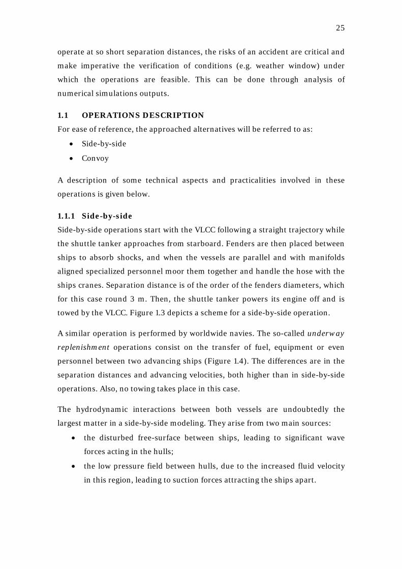
Figure 1.3 - Side-by-side operation scheme. ........................................................ 26

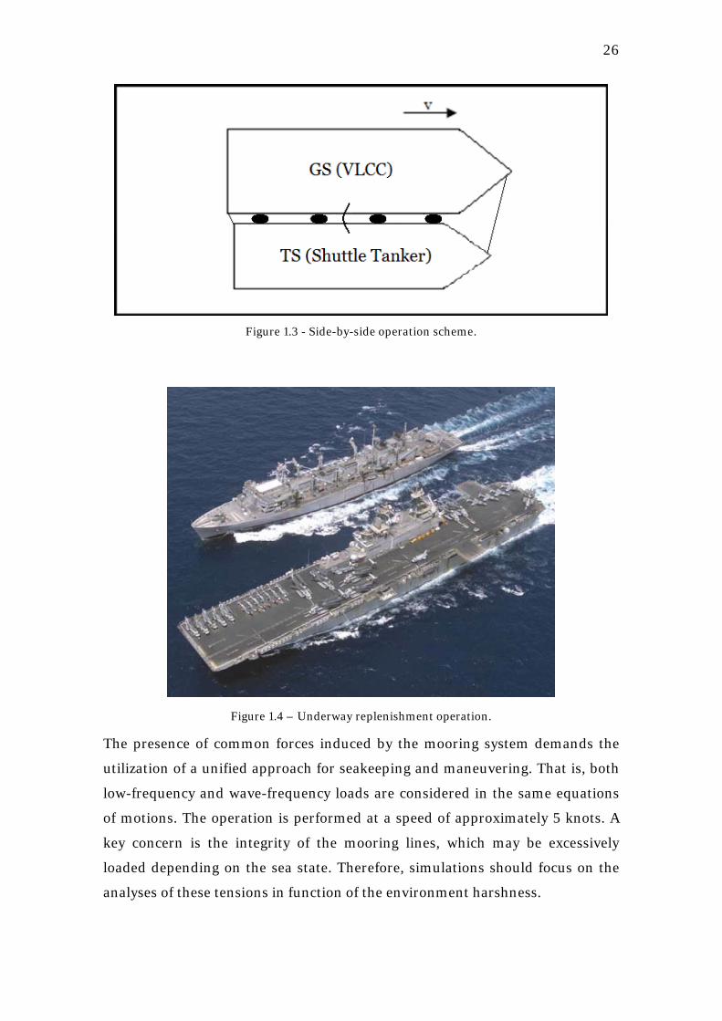
Figure 1.4 – Underway replenishment operation. ............................................... 26

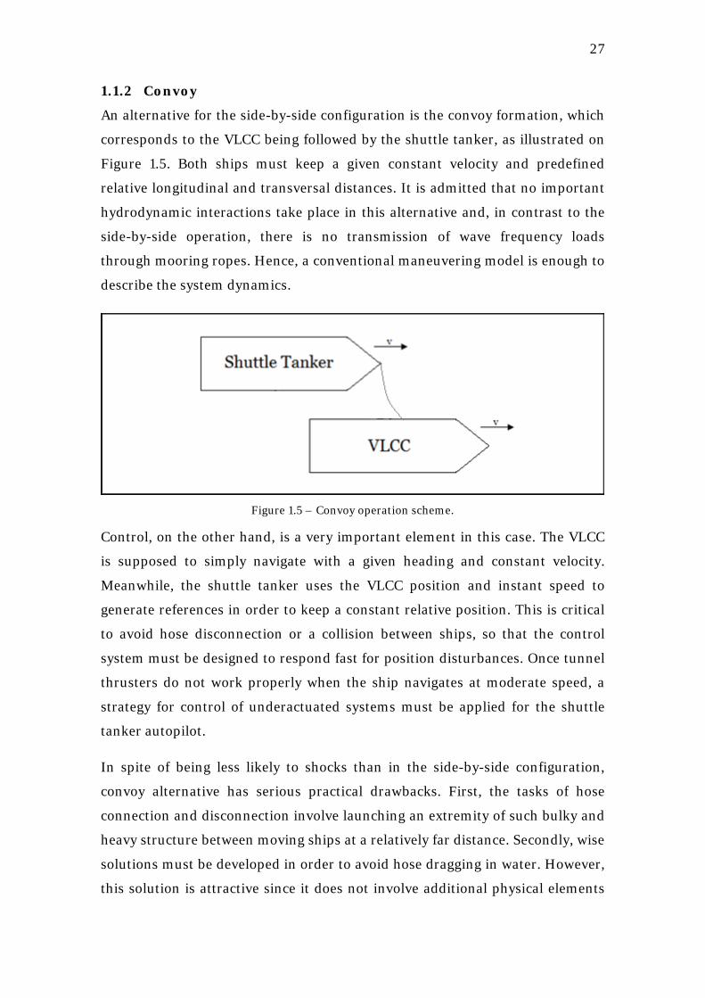
Figure 1.5 – Convoy operation scheme. ............................................................... 27

Figure 2.1 – Coordinate systems .......................................................................... 37

Figure 2.2 – Added mass (surge) for a tanker versus frequency of encounter. .. 48

Figure 2.3 – Comparison between JONSWAP and Pierson-Moskowitz spectra.

................................................................................................................. 53

Figure 2.4 – RAOs for sway (left) and yaw (right) motions for a pipelaying barge

and for a 100% loaded VLCC .................................................................. 53

Figure 2.5 – Illustration of the process of transforming wave elevation in ship

motions .................................................................................................... 54

Figure 2.6 – Wind coefficients (surge) versus incidence direction. .................... 57

Figure 2.7 – Wind coefficients (sway) versus incidence direction. ..................... 58

Figure 2.8 – Wind coefficients (yaw) versus incidence direction. ...................... 58

Figure 2.9 – Usual approach of superposing LF and WF motions ..................... 64

Figure 2.10 – Unified model for maneuvering and seakeeping .......................... 68

Figure 3.1 – PID controller structure. .................................................................. 70

Figure 3.2 – Integrator windup phenomenon, where 𝑦 is the process output, 𝑦𝑠𝑑

is the setpoint, 𝑢 is the control signal and 𝐼 is the integral part.

Extracted from ........................................................................................ 71

Figure 3.3 – Line-of-sight procedure for calculation of 𝜓𝑟𝑒𝑓. ........................... 80

Figure 4.1 – Side-by-side operation ..................................................................... 81

Figure 4.2 – Maneuvering and berthing. ............................................................. 82

Figure 4.3 - Typical mooring scheme................................................................... 83

Figure 4.4 – Wave field between two approaching ships .................................... 85

Figure 4.5 – Ships advancing in waves. ............................................................... 87

Figure 4.6 – A lid (red) is placed between hulls for attenuation of the free-

surface elevation...................................................................................... 89

Figure 4.7 – Fenders avoid steel-steel contact between ships hulls.................... 92

Figure 4.8 – Fender model................................................................................... 93

Figure 4.9 – Fenders reaction forces X deflection percentage (top) and

displacement (bottom). ........................................................................... 94

Figure 5.1 - Convoy operation. ............................................................................. 98

Figure 6.1 – Mooring scheme. ............................................................................. 111

Figure 6.2 – Damped free surface elevation – for a unitary incident wave

amplitude – for loading condition 1. The x-axis corresponds to points

distributed along the lid length, with 0 and 38 corresponding to the aft-

and fore-most extremities, respectively. ............................................... 112

Figure 6.3 – Parametric approximation for the retardation function (VLCC –

surge-surge). .......................................................................................... 114

Figure 6.4 – Connection between the equations of motions and the state-space

system for approximation of the memory functions vector 𝛍. .............. 114

Figure 6.5 – Sway-sway hydrodynamic coefficients referent to the VLCC (A11,

B11), to the coupled effects on the VLCC due to the shuttle tanker

motions (A12, B12), to the coupled effects on the shuttle tanker due to

the VLCC motions (A21, B21) and to the shuttle tanker (A22, B22). .... 116

Figure 6.6 – Sway-sway added masses calculated for both isolated and

interacting ships. .................................................................................... 116

Figure 6.7 – XY positions for side-by-side operation under loading condition 1,

Hs = 3.5 m, Tp = 15.0s, wave incidence of 195º and mooring

arrangement 8-4-6. ............................................................................... 118

Figure 6.8 – Fender loads for side-by-side operation under loading condition 1,

Hs = 3.5 m, Tp = 15.0s, wave incidence of 195º and mooring

arrangement 8-4-6. ................................................................................ 119

Figure 6.9 – Traction in mooring lines for side-by-side operation under loading

condition 1, Hs = 3.5 m, Tp = 15.0s, wave incidence of 195º and mooring

arrangement 8-4-6. ............................................................................... 120

Figure 6.10 – Roll, pitch and yaw motions for side-by-side operation under

loading condition 1, Hs = 3.5 m, Tp = 15.0s, wave incidence of 195º and

mooring arrangement 8-4-6. ................................................................ 120

Figure 6.11 – Mooring system conditions for side-by-side operation under

loading condition 1, wave incidence of 195º and mooring arrangement

8-4-6. ...................................................................................................... 121



8-4-6. ..................................................................................................... 122



8-4-4. ..................................................................................................... 122



8-4-4. ..................................................................................................... 122

Figure 6.15 – Roll, pitch and yaw motions for side-by-side operation under

loading condition 1, Hs = 3.5 m, Tp = 15.0s, wave incidence of 195º and

mooring arrangement 8-4-4. ................................................................ 123



6-4-4. ..................................................................................................... 123



6-4-4. ..................................................................................................... 123



8-4-6. ..................................................................................................... 123



8-4-6. ..................................................................................................... 124



8-4-4. ..................................................................................................... 124



8-4-4. ..................................................................................................... 124



6-4-4. ..................................................................................................... 124



6-4-4. ..................................................................................................... 125



8-4-6. ..................................................................................................... 125

Figure 6.25 – Mooring system for side-by-side operation under loading

condition 3, wave incidence of 315º and mooring arrangement 8-4-6.

............................................................................................................... 125



8-4-4. ..................................................................................................... 125



8-4-4. ..................................................................................................... 126



6-4-4. ..................................................................................................... 126



6-4-4. ..................................................................................................... 126

Figure 6.30 – Rudder lift coefficient for the shuttle tanker. ............................. 128

Figure 6.31 – Distance between manifolds 𝐷𝑚𝑓. .............................................. 130

Figure 6.32 – XY positions for convoy operation under loading condition 1, Hs =

1.5m, Tp = 8.0s, wave incidence 195º and no wind loads. ..................... 131

Figure 6.33 – Distance between manifolds for convoy operation under loading

condition 1, Hs = 1.5m, Tp = 8.0s, wave incidence 195º and no wind

loads. ...................................................................................................... 131

Figure 6.34 – Low-frequency estimates for convoy operation under loading

condition 1, Hs = 1.5m, Tp = 8.0s, wave incidence 195º and no wind

loads. ..................................................................................................... 132

Figure 6.35 - Rudder commanded and effective deflection for convoy operation

under loading condition 1, Hs = 1.5m, Tp = 8.0s, wave incidence 195º

and no wind loads. ................................................................................ 132

Figure 6.36 – Results for convoy operation under loading condition 1, wave

incidence of 120º and in presence of wind. .......................................... 133


incidence of 120º and in absence of wind. ........................................... 133

Figure 6. 38 – Results for convoy operation under loading condition 1, wave



incidence of 195º and in absence of wind. ............................................ 134

























LIST OF TABLES

Table 2.1 – Notation for generalized positions, velocities and forces. ................ 35

Table 6.1 – VLCC main dimensions. .................................................................. 107

Table 6.2 – Shuttle tanker main dimensions. .................................................... 108

Table 6.3 –Compression X induced force relation for fenders. ........................ 110

Table 6.4 – Mooring lines properties. ................................................................ 111

Table 6.6 – Main properties of the shuttle tanker rudder. ................................ 127

Table 6.7 – Waves parameters for the convoy simulations. .............................. 129

LIST OF SYMBOLS

Vectors and matrices are written in bold characters, while scalars are generally

in italic. When the same symbol is assigned to two or more distinct meanings, a

subscript is placed in at least one of them for sake of distinction. Following, the

most relevant adopted in this symbols are presented as to ease consultation

throughout the text reading.

Roman alphabet

𝐀 Added mass and inertia matrix

𝐀(∞) Asymptotic infinite-frequency added mass matrix

𝐀0 Zero-frequency added mass matrix

𝐴𝐿 Lateral ship projected area above water surface

𝐴𝑟 Rudder area

𝐴𝑇 Transverse ship projected area above water surface

𝐀𝐫 State matrix for the memory effects state-space

approximation

𝐴𝑤𝑝 Water plane area

𝐛 Bias forces and moments vector

𝐁 Potential damping matrix

𝐁𝐫 Input matrix for the memory effects state-space

approximation

𝐵𝑠 Ship beam

𝐂𝐴 Added mass Coriolis and centripetal matrix

𝐶𝐵 Block coefficient

𝐶ℎ,𝑖 Coefficient for calculation of hydrodynamic suction loads

(𝑖 = 𝑋,𝑌,𝑁)

𝐶𝑖,𝑐𝑢𝑟𝑟 Coefficient for calculation of current loads (𝑖 = 𝑋,𝑌,𝑁)

𝐶𝑖,𝑤𝑖𝑛𝑑 Coefficient for calculation of wind loads (𝑖 = 𝑋,𝑌,𝑁)

𝐶𝐿 Rudder lift coefficient

𝑐𝑚 Rudder mean chord

𝐂𝐫 Output matrix for the memory effects state-space

approximation

𝐂𝑅𝐵 Rigid-body Coriolis and centripetal matrix

𝐝 Vector of damping loads

𝑑𝐿 Longitudinal distance assigned for the convoy operation

𝑑𝑇 Transversal distance assigned for the convoy operation

𝐷𝑖 Drift coefficient (𝑖 = 1,2,6)

𝐷𝑚𝑓 Distance between manifolds

𝐷𝑝 Propeller diameter

𝐷𝑟𝑜𝑝𝑒 Mooring rope diameter

𝐷𝑠 Ship depth

𝐷𝑤𝑑𝑑,𝑖 Wave drift damping coefficient (𝑖 = 1,2,6)

𝐃 Damping matrix

𝐃𝐫 Feedthrough matrix for the memory effects state-space

approximation

𝑓 Ship freeboard

𝐹𝑖𝑀𝐷 Waves mean drift forces (𝑖 = 1,2,6)

𝐹𝑛 Froud number

𝑔 Acceleration of gravity

𝐠 Vector of restoration loads

𝐆 Restoration matrix

𝐺𝑀��𝐿 Longitudinal metacentric height

𝐺𝑀��𝑇 Transversal metacentric height

𝐺𝑃𝐼𝐷 PID controller transfer function

ℎ𝑟 Rudder height

𝐻𝑠 Significant wave height

𝐼𝑖 Ship moment of inertia relative to i-axis (𝑖 = 𝑥,𝑦, 𝑧)

𝐼𝑖𝑗 Ship product of inertia (𝑖, 𝑗 = 𝑥,𝑦, 𝑧, 𝑖 ≠ 𝑗)

𝐉𝐛𝐧 Coordinates rotation matrix from body- to Earth-fixed

systems

𝑘 Wave number

K Moment in roll direction

𝐊 Matrix of retardation functions

𝐊1 Gain matrix for the observer wave-frequency model

𝐊2 Gain matrix for the observer kinematics model

𝐾𝑟𝑜𝑝𝑒 Mooring rope stiffness

𝑙ℎ Hose length

𝑙𝛿 Moment arm from the ship center of gravity to the rudder

center of pressure

𝐿𝑜𝑎 Length overall

𝐿𝑝𝑝 Length between perpendiculars

𝐿𝑟𝑜𝑝𝑒 Mooring rope length

𝑚 Ship mass

M Moment on pitch direction

𝐌 Inertia matrix

𝐌𝑅𝐵 Rigid-body inertia matrix

N Moment on yaw direction

𝑁𝑐𝑢𝑟𝑟 Current moment in yaw

𝑁𝑤𝑖𝑛𝑑 Wind moment in yaw

ob Origin of the body-fixed coordinate system

on Origin of the Earth-fixed coordinate system

0s Origin of the seakeeping coordinate system

p Angular velocity in roll

𝑝𝑙𝑜𝑠 Line-of-sight position

q Angular velocity in pitch

r Angular velocity in yaw

𝐑𝑎𝑏 Matrix for rotation of a vector in frame a to a frame b

𝑅𝑒 Reynolds number

𝑆𝑠 Ship wetted hull area

𝑆𝑤 Wave spectrum

𝐓 Matrix with time constants for the bias model

𝐓𝑎 Euler angles attitude matrix

𝑇𝑚𝑎𝑥 Main propeller maximum thrust

𝑇𝑚𝑖𝑛 Main propeller minimum thrust

𝑇𝑝 Wave peak period

𝑇𝑟𝑜𝑝𝑒 Mooring rope traction

𝑇𝑠 Ship draft

u Linear velocity in surge

Greek alphabet

𝑢𝑟𝑒𝑓 Surge velocity reference

𝑈𝑐𝑢𝑟𝑟 Current speed

𝑈𝑠 Service speed

𝑈𝑤𝑖𝑛𝑑 Wind speed

v Linear velocity in sway

w Linear velocity in heave

𝐰 Vector of zero-mean gaussian white noise

x Position in surge direction

y Position in sway direction

z Position in heave direction

X Force in surge direction

𝑋𝑐𝑢𝑟𝑟 Current force in surge

𝑋𝑖𝑊𝐹 1st –order wave load (𝑖 = 1,2,6)

𝑋𝑤𝑖𝑛𝑑 Wind force in surge

Y Force in sway direction

𝑦𝑚𝑖𝑛 Minimum safe separation distance assigned for the

convoy operation

𝑦𝑠𝑒𝑝 Separation distance assigned for the convoy operation

𝑌𝑐𝑢𝑟𝑟 Current force in sway

𝑌𝑤𝑖𝑛𝑑 Wind force in sway

Z Force in heave direction

𝛼𝑟 Current relative incidence direction

𝛽𝑟 Wave relative incidence direction

𝛾𝑟 Wind relative incidence direction

𝛿𝑟 Rudder deflection

Δ Ship displacement

𝚪 Output matrix for the observer wave-frequency model

𝜁𝑖 Damping for the observer wave model (𝑖 = 1,2,3)

𝜁𝑛𝑖 Notch filter damping for the observer wave model

(𝑖 = 1,2,3)

𝛈 Vector with 6 DOF coordinates in the Earth-fixed system

𝛈1 Vector of positions in the Earth-fixed system

𝛈2 Vector of Euler angles in the Earth-fixed system

𝛈ℎ Vector with horizontal 3 DOF coordinates in the Earth-

fixed system

𝛈𝑆𝐵𝑆 Coupled vector of coordinates for the side-by-side model

𝜼𝑤𝑓 Vector of wave-frequency positions

θ Euler angle respective to pitch

𝛋 Gain matrix for the observer low-frequency model

𝜆𝑒 Wave-length of encounter

𝜆𝑝𝑟𝑜𝑗 Projection of the wave-length in the ship advance

direction

𝚲 Gain matrix for the observer bias model

Λ𝑔 Rudder effective aspect ratio

𝛍 Vector of memory effects

𝛎 Vector with 6 DOF velocities in the body-fixed system

𝛎1 Vector of linear velocities in the body-fixed system

𝛎2 Vector of angular velocities in the body-fixed system

𝛎ℎ Vector with horizontal 3 DOF velocities in the body-fixed

system

𝛎𝑆𝐵𝑆 Coupled vector of velocities for the side-by-side model

𝛏 Vector with 6 DOF coordinates in the seakeeping system

ξi Coordinate in i-direction (𝑖 = 1, … ,6) of the seakeeping

system

𝜌𝐴𝑖𝑟 Density of air

𝜌𝑤 Density of water

𝜎𝑖 Parameter for adjustment of the observer wave model

(𝑖 = 1,2,3)

𝜎𝑟𝑜𝑝𝑒 Mooring rope tension

𝚺 Input matrix for the observer wave-frequency model

𝛕 Vector with 6 DOF loads in the body-fixed system

𝛕1 Vector of forces in the body-fixed system

𝛕2 Vector of moments in the body-fixed system

Other symbols and notation

𝛕𝑐𝑡𝑟 Vector of control loads

𝛕𝑏𝑎𝑐𝑘𝑠 Vector of control loads determined by the backstepping

controller

𝛕𝑒𝑛𝑣 Vector of environmental loads

𝝉𝑓𝑛𝑑 Vector of fender loads

𝝉ℎ𝑑𝑙 Vector of hydrodynamic suction loads

𝛕ℎ𝑦𝑑 Vector of hydrodynamic loads

𝝉𝑚𝑟𝑛 Vector of mooring system loads

𝜏𝑃𝐼𝐷 PID controller load

𝝉𝑊𝐹 Vector of first-order wave loads

φ Euler angle respective to roll

𝛘 State vector for the memory effects approximation

ψ Euler angle respective to yaw

𝜓𝑟𝑒𝑓 Heading reference

𝜔 Wave frequency

𝜔0𝑖 Modal frequency for the observer wave model (𝑖 = 1,2,3)

𝜔𝑐𝑖 Cut frequency for the observer wave model (𝑖 = 1,2,3)

𝜔𝑒 Frequency of encounter

𝜔𝑝 Wave peak frequency

𝛀 State matrix for the observer wave-frequency model

∇ Ship volumetric displacement

∙ (over the symbol) Time derivation

T (superscript) Transposed matrix

∧ (over the symbol) Estimated value

~ (over the symbol) Offset between real and desired values

− (over the symbol) Offset between real and estimated

values

Quem bater primeiro a dobra do mar

Dá de lá bandeira qualquer

Aponta pra fé e rema

“Dois Barcos”, Marcelo Camelo

22

1. INTRODUCTION Oil production in Brazil is expected to increase considerably in the next decades.

In a moment characterized by increase in consumption and depletion of many

of the current proven reserves, exploration of the Pre-salt fields is supposed to

put the country among prominent oil exporters. In fact, world oil demand is

presumed to increase from 94 mb/d1

The important role Brazil is going to play in the oil industry makes it

indispensable to start the development of solutions for a wide spectrum of

challenges. Pre-salt oil fields lie at high depths and up to 300 km far from the

coast. Thus, optimal usage of resources is imperative to ensure economic

viability in the exploitation process. Advanced technology will be required in

many operations, leading to high costs in virtually every stage of the production.

In this sense, any solution that may lead to a more efficient utilization of the

exploitation equipment, oil rigs and ships is very welcome.

in 2015 to 106 mb/d in 2030, while the

output at the current producing fields is going to drop from 51 mb/d in 2015 to

27 mb/d in 2030 (IEA, 2008). Thus, production in new fields will be vital to

supply world demand for energy in the next decades.

The present work focuses on alternatives to improve the utilization of shuttle

tankers. These ships, usually provided with dynamic positioning systems, are

broadly used in offloading operations, which consist in the transfer of oil from a

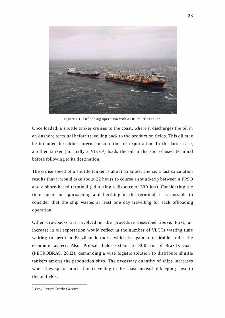
FPSO2 Figure 1.1 to a tanker ( ).

Dynamic positioning (DP) systems are intended to control a ship in surge, sway

and yaw motions exclusively by means of thrusters (FOSSEN, 2002). They are

important during an offloading operation in order to keep the shuttle tanker –

subjected to environment action – with a safe position relative to the FPSO,

avoiding incidents like shocks and hose disconnections. However, a DP system

considerably increases the costs of a ship, such that a so-called DP shuttle

tanker should be used in a very rational way in order to diminish the total

expenses involved in the supply chain.

1 Million barrels per day. 2 Acronym for Floating, Production, Storage and Offloading unity. Roughly speaking, this is a kind of platform capable of both explore and keep oil until it is offloaded to the shuttle tanker.

23

Figure 1.1 - Offloading operation with a DP-shuttle tanker.

Once loaded, a shuttle tanker cruises to the coast, where it discharges the oil in

an onshore terminal before travelling back to the production fields. This oil may

be intended for either intern consumption or exportation. In the latter case,

another tanker (normally a VLCC3

The cruise speed of a shuttle tanker is about 15 knots. Hence, a fast calculation

results that it would take about 22 hours to course a round-trip between a FPSO

and a shore-based terminal (admitting a distance of 300 km). Considering the

time spent for approaching and berthing in the terminal, it is possible to

consider that the ship wastes at least one day travelling for each offloading

operation.

) loads the oil in the shore-based terminal

before following to its destination.

Other drawbacks are involved in the procedure described above. First, an

increase in oil exportation would reflect in the number of VLCCs wasting time

waiting to berth in Brazilian harbors, which is again undesirable under the

economic aspect. Also, Pre-salt fields extend to 800 km of Brazil’s coast

(PETROBRAS, 2012), demanding a wise logistic solution to distribute shuttle

tankers among the production sites. The necessary quantity of ships increases

when they spend much time travelling to the coast instead of keeping close to

the oil fields.

3 Very Large Crude Carrier.

24

A worthy alternative to overcome these disadvantages would be to avoid the

time-consuming trips, by transferring the oil intended to exportation from the

shuttle tanker directly to the VLCC. This could be performed around the

exploration fields, so that at the end of the transfer process the shuttle tanker

would already be close to the production units.

Obviously, the proposed solution is not free of caveats. In fact, as in any

conventional offloading operation, it is imperative to assure a safe relative

distance between ships, even under harsh environmental conditions. However,

in general a VLCC is not provided with a station keeping system like dynamic

positioning. Anchoring is also impracticable, considering that Pre-salt fields

may lie at up to 2000 m water depth. The risks involved in the transfer of oil

between two vessels in open sea make it indispensable to ensure controllability

for both of them.

Course controllability may be attained if ships advance at moderate speed. This

motivates the proposal of two different configurations for underway transfer of

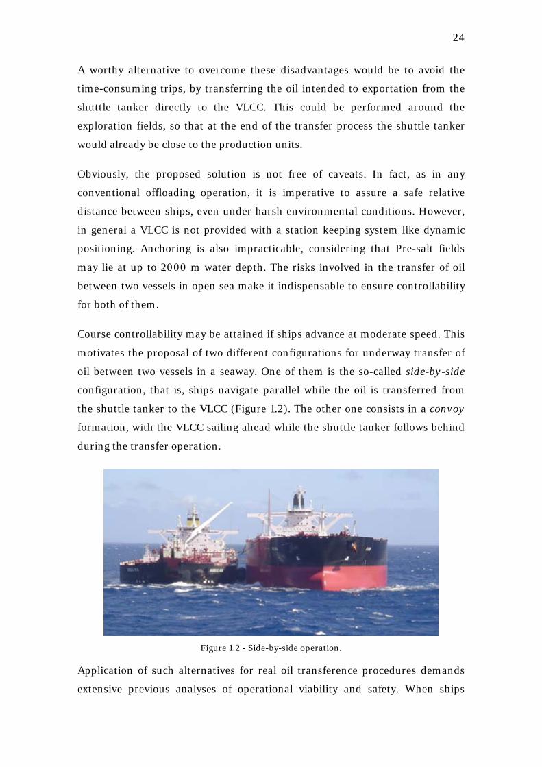
oil between two vessels in a seaway. One of them is the so-called side-by-side

configuration, that is, ships navigate parallel while the oil is transferred from

the shuttle tanker to the VLCC (Figure 1.2). The other one consists in a convoy

formation, with the VLCC sailing ahead while the shuttle tanker follows behind

during the transfer operation.

Figure 1.2 - Side-by-side operation.

Application of such alternatives for real oil transference procedures demands

extensive previous analyses of operational viability and safety. When ships

25

operate at so short separation distances, the risks of an accident are critical and

make imperative the verification of conditions (e.g. weather window) under

which the operations are feasible. This can be done through analysis of

numerical simulations outputs.

1.1 OPERATIONS DESCRIPTION

For ease of reference, the approached alternatives will be referred to as:

• Side-by-side

• Convoy

A description of some technical aspects and practicalities involved in these

operations is given below.

1.1.1 Side-by-side

Side-by-side operations start with the VLCC following a straight trajectory while

the shuttle tanker approaches from starboard. Fenders are then placed between

ships to absorb shocks, and when the vessels are parallel and with manifolds

aligned specialized personnel moor them together and handle the hose with the

ships cranes. Separation distance is of the order of the fenders diameters, which

for this case round 3 m. Then, the shuttle tanker powers its engine off and is

towed by the VLCC. Figure 1.3 depicts a scheme for a side-by-side operation.

A similar operation is performed by worldwide navies. The so-called underway

replenishment operations consist on the transfer of fuel, equipment or even

personnel between two advancing ships (Figure 1.4). The differences are in the

separation distances and advancing velocities, both higher than in side-by-side

operations. Also, no towing takes place in this case.

The hydrodynamic interactions between both vessels are undoubtedly the

largest matter in a side-by-side modeling. They arise from two main sources:

• the disturbed free-surface between ships, leading to significant wave

forces acting in the hulls;

• the low pressure field between hulls, due to the increased fluid velocity

in this region, leading to suction forces attracting the ships apart.

26

Figure 1.3 - Side-by-side operation scheme.

Figure 1.4 – Underway replenishment operation.

The presence of common forces induced by the mooring system demands the

utilization of a unified approach for seakeeping and maneuvering. That is, both

low-frequency and wave-frequency loads are considered in the same equations

of motions. The operation is performed at a speed of approximately 5 knots. A

key concern is the integrity of the mooring lines, which may be excessively

loaded depending on the sea state. Therefore, simulations should focus on the

analyses of these tensions in function of the environment harshness.

27

1.1.2 Convoy

An alternative for the side-by-side configuration is the convoy formation, which

corresponds to the VLCC being followed by the shuttle tanker, as illustrated on

Figure 1.5. Both ships must keep a given constant velocity and predefined

relative longitudinal and transversal distances. It is admitted that no important

hydrodynamic interactions take place in this alternative and, in contrast to the

side-by-side operation, there is no transmission of wave frequency loads

through mooring ropes. Hence, a conventional maneuvering model is enough to

describe the system dynamics.

Figure 1.5 – Convoy operation scheme.

Control, on the other hand, is a very important element in this case. The VLCC

is supposed to simply navigate with a given heading and constant velocity.

Meanwhile, the shuttle tanker uses the VLCC position and instant speed to

generate references in order to keep a constant relative position. This is critical

to avoid hose disconnection or a collision between ships, so that the control

system must be designed to respond fast for position disturbances. Once tunnel

thrusters do not work properly when the ship navigates at moderate speed, a

strategy for control of underactuated systems must be applied for the shuttle

tanker autopilot.

In spite of being less likely to shocks than in the side-by-side configuration,

convoy alternative has serious practical drawbacks. First, the tasks of hose

connection and disconnection involve launching an extremity of such bulky and

heavy structure between moving ships at a relatively far distance. Secondly, wise

solutions must be developed in order to avoid hose dragging in water. However,

this solution is attractive since it does not involve additional physical elements

28

for controllability – the only demand is the implementation of the proper

control algorithm for the shuttle tanker autopilot system.

1.2 LITERATURE REVIEW

The deduction and understanding of the ship equations of motions demand a

mature treatment of rigid-body dynamics. This is properly presented in

(FOSSEN, 1994, 2002), where a vectorial approach is used to describe the ship

kinematics and dynamics, leading to the equations of motion in 6 DOF. A

rigorous kinematics treatment involving three coordinate frames is given in

(PEREZ and FOSSEN, 2007). A basis on dynamics of linear systems is provided

in (MEIROVITCH, 1970).

Another key topic for a proper comprehension of ship motions is

hydrodynamics. A theoretical treatment devoted to marine systems is

extensively covered in (NEWMAN, 1977), and (FALTINSEN, 1990) is a valuable

reference on the effects of sea loads in floating structures.

The choice of proper environmental models is essential for ship dynamics

modeling. A quasi-explicit4

Wave loads are calculated by means of coefficients and transfer functions

provided by potential theory software based on the panels method, as explained

on (WAMIT, 2006). A method for calculation of wave drift loads with influence

of wave-current interaction is presented in (ARANHA, 1996), but this approach

is not adequate for the case of two close ships advancing parallelly.

heuristic model for estimating current loads on

static ships is presented in (LEITE, ARANHA, et al., 1998), and is extended in

(SIMOS, TANNURI and ARANHA, 2001) to incorporate yaw damping terms.

For both wind and current loads in tankers, (OCIMF, 1977) is considered to be a

standard method due to its simplicity and coherent estimates. However, when

two ships operate close from each other it is important to consider wind

shadowing effects. Some investigations are available for the tandem

configuration, like (BUCHNER and BUNNIK, 2002) and (TANNURI, FUCATU,

et al., 2010), but no works were found for the specific case of the side-by-side

configuration.

4 That is, dependent on the ship’s main dimensions and only a few hydrodynamic coefficients.

29

Ship dynamics are usually divided in maneuvering and seakeeping theories.

Both topics are overviewed on (PEREZ, FOSSEN and SøRENSEN, 2004) and

more extensively on (LEWIS, 1998). Maneuvering is specifically considered in

(SKJETNE, 2005) and (SKJETNE, SMOGELI and FOSSEN, 2004), where it is

treated in a control-oriented point-of-view. Models based on hydrodynamic

derivatives are widely used for maneuvering simulations. Descriptions of this

approach are given in (NORRBIN, 1970), (INOUE, HIRANO and KIJIMA,

1981), (BERTRAM, 2000), (VAN BERLEKOM and GODDARD, 1972) and

(PEREZ and BLANKE, 2008).

Some situations, however, demand the use a unified model for both

maneuvering and seakeeping (BAILEY, PRICE and TEMAREL, 1997). This is

the case when common forces are present in a multibody system, so that wave

frequency loads are transmitted between ships. This leads to consideration of

fluid memory effects on the equations of motions, represented by convolution

integrals of retardation functions (CUMMINS, 1962), (OGILVIE, 1964). A

formulation for the complete set of nonlinear equations of motions formulated

for the unified model is presented in (FOSSEN, 2005).

At first sight, the unified model may be considered unviable for time-domain

simulations due to the convolution integral to be evaluated at every time-step.

This problem may be overcome by replacing the integral by a linear state-space

model, with matrices determined by identification of a parametric

representation of the convolution term (KRISTIANSEN and EGELAND, 2003),

(HJUSTAD, KRISTIANSEN and EGELAND, 2004) and (KAASEN and MO,

2005). Several publications explain how to deal with this task in practice,

(PEREZ and FOSSEN, 2009), (PEREZ and FOSSEN, 2009) and (TAGHIPUR,

PEREZ and MOAN, 2008).

An alternative method for considering a unified model for maneuvering and

seakeeping is the two-time scale model proposed in (SKEJIC, 2008) and

(SKEJIC and FALTINSEN, 2008). This approach consists in considering the

linear wave-induced motions to occur in a faster time-scale than the

maneuvering dynamics, allowing the equations of motion for both seakeeping

and maneuvering to be solved separately but without disregarding their

interdependence.

30

A basis on linear control systems theory is provided in (DORF and BISHOP,

2001). It covers a wide range of subjects from frequency domain analysis to

state-space systems, including classical control approaches and the most

commonly used methods to determine stability. Nonlinear control is treated in a

somewhat applied point of view in (MÁRQUEZ, 2003), while a deeper

understanding on nonlinear systems theory for control purposes may be found

in (KHALIL, 2001). (KRSTIC, KANELLAKOPOULOS and KOKOTOVIC, 1995)

presents the backstepping methodology for nonlinear control. (FOSSEN, 1994),

(FOSSEN, 2002) and (SøRENSEN, 2005) are first references on application of

control methods to marine systems. Application of nonlinear controllers to

ships is covered in (FOSSEN and STRAND, 1998), and in (FOSSEN and

STRAND, 1999) nonlinear observers design based on passivity theory is

explored. A survey on industrial systems for guidance and control of ships is

presented in (GOLDING, 2004).

Underway side-by-side operations are for some extent becoming popular in the

oil industry. Safety procedures in such operations are provided in a guideline

published by OCIMF5

The behavior of the wave field between two ships in underway replenishment is

modeled by means of potential theory in (CHEN and FANG, 2001). The

influence of a ship motions due to the presence of a second one, also in

underway replenishment, is investigated in (MCTAGGART, CUMMING, et al.,

2003). QUADVLIEG et al. (2011) describe the side-by-side case, where the very

short clearance influences even more on the free-surface between ships than in

the underway replenishment case.

(OCIMF, 2005). An overview of side-by-side operations is

presented in (BERG and BAKKE, 2008), and a dynamic model is proposed in

(SOUZA and MORISHITA, 2011). Criteria for fenders selection and mooring

arrangements are described in (SAKAKIBARA and YAMADA, 2008). Obviously,

the hydrodynamic interactions comprise a main source of worries for this

configuration. The number of publications and conferences approaching this

area is increasing, but there is still a lack of conclusive answers and methods

concerning the phenomenon.

5 Oil Companies International Marine Forum.

31

Potential theory-based software overestimate the wave elevation between close

ships, since they disregard important viscous effects and thus lead to undamped

resonant modes on the calculated wave elevation between the vessels. This

problem may be overcame through modeling of a “lid” over the gap between the

ships hulls, that is, an additional structure considered in the hydrodynamic

calculations whose motions emulate the free surface elevation (BUCHNER,

VAN DIJK and DE WILDE, 2001).

Models for the suction and repulsion forces that appear when two ships navigate

parallel in calm water are available, but almost always refer to the case of

maneuvering in channels, corresponding thus to shallow water. Some of them

are (VARYANI, THAVALINGAM and KRISHNANKUTTY, 2004), where a

model for calculating interaction loads is proposed and (VANTORRE,

VERZHBITSKAYA and LAFORCE, 2002), which presents formulations based

on model tests. (DE DECKER, 2006) used experimental shallow water data to

develop a model for the side-by-side case, that is, with zero-relative speed.

Analytical solutions are proposed in (WANG, 2007) and (XIANG and

FALTINSEN, 2011).

The main concern for the convoy formation relates to the control of an

underactuated system. Therefore, control of lateral motions is done indirectly by

the shuttle tanker autopilot, whose heading references are generated through

the line-of-sight guidance method. This is described in (BREIVIK, 2003) and

(FOSSEN, BREIVIK and SKJETNE, 2003). Since the trajectory of the shuttle

tanker is defined by the VLCC motions, the problem is one of way-point

tracking, which is treated in (BREIVIK, HOVSTEIN and FOSSEN, 2008). These

references also propose control strategies for both surge velocity and yaw

moment. A problem involving path-following and maintenance of a given

formation pattern is treated in (SOUZA, OSHIRO and MORISHITA, 2010).

However, it relates to a very low-speed situation, so that all ships may control

their horizontal positions by means of tunnel thrusters.

1.3 OBJECTIVES

The purpose of the present work is to analyze the viability of two different

alternatives of oil transfer between two ships in open sea, viz, side-by-side and

convoy configurations. The task is divided into three main stages:

32

a. Development of dynamic models and control approaches for two

different configurations of ship-to-ship oil transfer operations in a

seaway, viz.: side-by-side and convoy formation.

b. Implementation of numerical simulators based on the resultant models.

c. Analysis of the results and conclusions about the feasibility of each

configuration, based on environmental conditions and operational

aspects (e.g. mooring arrangements, thrusters’ capacity, etc).

Once each situation demands a different approach for dynamics and control, it

may be more convenient to list the objectives for each operation individually:

Side-by-side

• Formulation of the nonlinear equations of motions in 6 degrees of

freedom correspondent to a unified approach for both maneuvering and

seakeeping.

• Development of models for the loads involved in the operation, viz.,

hydrodynamic interaction loads, fenders, mooring system and

environment.

• Discussion about the calculation of hydrodynamic data for ships in

interaction.

• Design of a control law for surge and yaw motions of the guide ship.

• Time-domain simulations for different environmental conditions,

mooring arrangements and loading conditions. Analysis of the mooring

lines tractions during the operation and determination of the suitable

mooring arrangements for a given environmental condition.

Convoy

• Development of a maneuvering model based on hydrodynamic

derivatives, including environmental action.

• Design of an autopilot for the shuttle tanker, based on the line-of-sight

strategy, a backstepping controller and nonlinear controller observer.

• Simulations for test of the LOS-based autopilot, considering different

incidence and harshness of the environmental agents, in order to verify if

the shuttle tanker autopilot is able to properly follow the VLCC without

hose disconnection or collisions.

33

1.4 TEXT ORGANIZATION

The necessary theoretical background for the development of dynamic modeling

is considered in Chapter 2. It starts presenting the adopted notation, following

with coordinate systems, kinematics and rigid-body dynamics. Then, basic

hydrodynamics are discussed, followed by a review on environmental loads and

models for their consideration in the ship dynamics. Finally, the 6 DOF

equations of motions for maneuvering and seakeeping are derived, followed by a

unified model for both approaches.

Chapter 3 introduces notions of control systems design. The PID controller is

presented, followed by the nonlinear backstepping control strategy. Then, a

nonlinear observer based on passivity theory is presented, and the chapter ends

with a description of the line-of-sight method for guidance, which is used in the

convoy formation operation.

Underway side-by-side operations are particularly considered in Chapter 4. An

overview of a complete operation is briefly presented, followed by a discussion

on the hydrodynamics interactions and the introduction of methods for

calculating the hydrodynamic data. Then, the operation modeling is developed.

The coupled equations of motions for the unified maneuvering and seakeeping

approach are written, and models for hydrodynamic interaction, fenders,

mooring system and environment are proposed.

The convoy operation is detailed in Chapter 5. First, the maneuvering model

introduced in Chapter 4 is adapted to be applied with a model of hydrodynamic

derivatives. Then, the algorithm for references generation is proposed, and the

control approaches presented on Chapter 3 are utilized for development of the

shuttle tanker autopilot system. The chapter ends with models for the actuators

dynamics.

Simulations procedures and their respective results are exposed on Chapter 6.

The ships dimensions for all loading cases are presented, and the combinations

of drafts – and, consequently, freeboards – are listed for each loading condition.

Following, simulations results for the side-by-side operation are presented, and

all the same is done for the convoy operation. Final considerations and

suggestions for future works are presented on Chapter 7.

34

2. DYNAMIC MODELING

Modeling of ship dynamics involves an elaborate combination of rigid-body

theory and hydrodynamics. In fact, ship motions are intrinsically complex due

to their highly coupled character and to the complicated response of a vessel to

its interaction with the surrounding fluid. Thus, a reasonable comprehension on

the physical origins of the forces and moments acting on the system is

imperative for a clear understanding and mathematical description of the

motions.

Ship motions may hardly be analyzed by means of a single system of

coordinates. It is convenient to approach each sort of problem with an

appropriate frame, such that distinct systems are usually utilized. Therefore, it

is necessary to establish a clear relation between the coordinates of different

frames, allowing the solutions obtained for one of them to be straightforwardly

related to the other one.

Environment plays an important role in ship dynamics and must be considered

in the dynamics formulation through the usage of reliable models available in

the literature. Furthermore, it is also interesting to have some comprehension

on the way such environment agents disturb the system, such that these models

may be properly applied to the model.

Usually, ship dynamics are divided into two main areas of study, viz.,

maneuvering and seakeeping. The first of them comprises the analysis of a

vessel response to its control surfaces (like rudders and similar), propulsion

system and low-frequency environment loads. Water is admitted to be calm,

that is, no 1st order wave loads are considered. Seakeeping, on the other hand,

refers to the behavior of a ship when excited by waves. Sometimes, however, the

practice of separating maneuvering from seakeeping does not comply with the

requirements of the problem, such that a unified approach should be used.

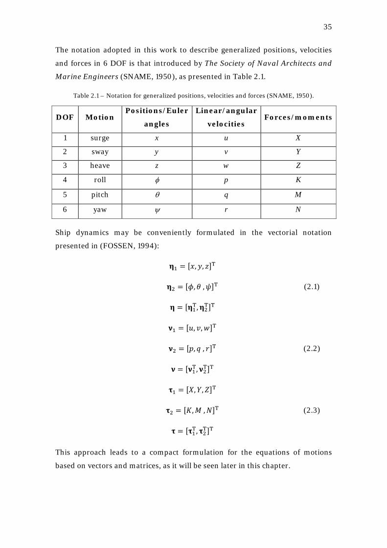
2.1 NOTATION

The position and motion of a rigid-body in space are described in 6 degrees of

freedom (DOF). Therefore, 6 independent variables are necessary to model a

ship moving in the ocean. Three of them are used to assign the position, while

the other three define the ship angles of orientation.

35

The notation adopted in this work to describe generalized positions, velocities

and forces in 6 DOF is that introduced by The Society of Naval Architects and

Marine Engineers (SNAME, 1950), as presented in Table 2.1.

Table 2.1 – Notation for generalized positions, velocities and forces (SNAME, 1950).

DOF Motion Positions/Euler

angles

Linear/angular

velocities Forces/moments

1 surge x u X

2 sway y v Y

3 heave z w Z

4 roll φ p K

5 pitch θ q M

6 yaw ψ r N

Ship dynamics may be conveniently formulated in the vectorial notation

presented in (FOSSEN, 1994):

𝛈1 = [𝑥,𝑦, 𝑧]T

𝛈2 = [𝜙,𝜃 ,𝜓]T

𝛈 = [𝛈1T,𝛈2T]T

(2.1)

𝛎1 = [𝑢, 𝑣,𝑤]T

𝛎2 = [𝑝, 𝑞 , 𝑟]T

𝛎 = [𝛎1T, 𝛎2T]T

(2.2)

𝛕1 = [𝑋,𝑌,𝑍]T

𝛕2 = [𝐾,𝑀 ,𝑁]T

𝛕 = [𝛕1T, 𝛕2T]T

(2.3)

This approach leads to a compact formulation for the equations of motions

based on vectors and matrices, as it will be seen later in this chapter.

36

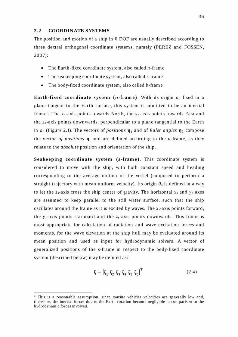
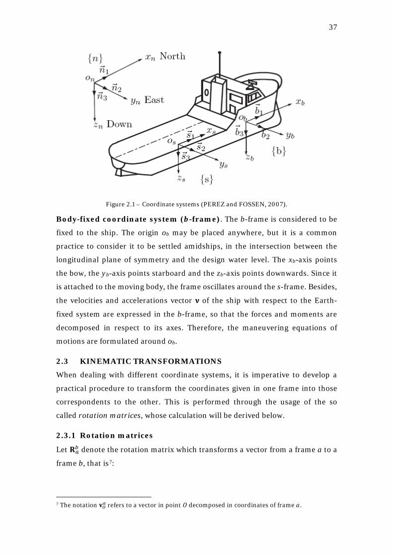
2.2 COORDINATE SYSTEMS

The position and motion of a ship in 6 DOF are usually described according to

three dextral orthogonal coordinate systems, namely (PEREZ and FOSSEN,

2007):

• The Earth-fixed coordinate system, also called n-frame

• The seakeeping coordinate system, also called s-frame

• The body-fixed coordinate system, also called b-frame

Earth-fixed coordinate system (n-frame). With its origin on fixed in a

plane tangent to the Earth surface, this system is admitted to be an inertial

frame6

Figure 2.1

. The xn-axis points towards North, the yn-axis points towards East and

the zn-axis points downwards, perpendicular to a plane tangential to the Earth

in on ( ). The vectors of positions 𝛈1 and of Euler angles 𝛈2 compose

the vector of positions 𝛈, and are defined according to the n-frame, as they

relate to the absolute position and orientation of the ship.

Seakeeping coordinate system (s-frame). This coordinate system is

considered to move with the ship, with both constant speed and heading

corresponding to the average motion of the vessel (supposed to perform a

straight trajectory with mean uniform velocity). Its origin 0s is defined in a way

to let the zs-axis cross the ship center of gravity. The horizontal xs and ys axes

are assumed to keep parallel to the still water surface, such that the ship

oscillates around the frame as it is excited by waves. The xs-axis points forward,

the ys-axis points starboard and the zs-axis points downwards. This frame is

most appropriate for calculation of radiation and wave excitation forces and

moments, for the wave elevation at the ship hull may be evaluated around its

mean position and used as input for hydrodynamic solvers. A vector of

generalized positions of the s-frame in respect to the body-fixed coordinate

system (described below) may be defined as:

𝛏 = �ξ1, ξ2, ξ3, ξ4, ξ5, ξ6�T

(2.4)

6 This is a reasonable assumption, since marine vehicles velocities are generally low and, therefore, the inertial forces due to the Earth rotation become negligible in comparison to the hydrodynamic forces involved.

37

Figure 2.1 – Coordinate systems (PEREZ and FOSSEN, 2007).

Body-fixed coordinate system (b-frame). The b-frame is considered to be

fixed to the ship. The origin ob may be placed anywhere, but it is a common

practice to consider it to be settled amidships, in the intersection between the

longitudinal plane of symmetry and the design water level. The xb-axis points

the bow, the yb-axis points starboard and the zb-axis points downwards. Since it

is attached to the moving body, the frame oscillates around the s-frame. Besides,

the velocities and accelerations vector 𝛎 of the ship with respect to the Earth-

fixed system are expressed in the b-frame, so that the forces and moments are

decomposed in respect to its axes. Therefore, the maneuvering equations of

motions are formulated around ob.

2.3 KINEMATIC TRANSFORMATIONS

When dealing with different coordinate systems, it is imperative to develop a

practical procedure to transform the coordinates given in one frame into those

correspondents to the other. This is performed through the usage of the so

called rotation matrices, whose calculation will be derived below.

2.3.1 Rotation matrices

Let 𝐑𝑎𝑏 denote the rotation matrix which transforms a vector from a frame a to a

frame b, that is7

7 The notation 𝐯𝑂𝑎 refers to a vector in point 𝑂 decomposed in coordinates of frame a.

:

38

𝐯o𝑏 = 𝐑𝑎𝑏𝐯o𝑎 (2.5)

The matrix 𝐑𝑎𝑏 is an element of 𝑆𝑂(3), that is, the set of special orthogonal

matrices of order 3:

𝑆𝑂(3) = {𝐀|𝐀 ∈ ℝ3X3,𝐀−1 = 𝐀T, det(𝐀) = 1} (2.6)

A rotation of frame b relative to frame a is called simple when it is performed

about a single axis. According to Euler’s theorem of rotation, it is possible to

describe any change in the relative orientation of two reference frames a and b

by means of a simple rotation of b about a. Therefore, if the rotation is

performed about an axis parallel to the unit vector 𝛌 = [𝜆1,𝜆2, 𝜆3] and by an

angle 𝛼, the rotation matrix 𝐑𝑎𝑏 may also be denoted as 𝐑𝜆,𝛼 and is calculated

according to (FOSSEN, 2002):

𝐑𝜆,𝛼 = 𝐈3X3 + sin(𝛼)𝐒(𝛌) + [1 − cos(α)]𝐒2(𝛌) (2.7)

where 𝐈3X3 is an identity matrix of order 3 and 𝐒(𝛌) is a skew-symmetric8

matrix

defined as:

𝐒(𝛌) = �0 −λ3 λ2λ3 0 −λ1−λ2 λ1 0

� (2.8)

Using formula (2.7), the simple rotations 𝜙, 𝜃 and 𝜓 about the n-frame axes xn,

yn and zn, respectively, may be performed through the following rotation

matrices:

𝐑𝑥𝑛,𝜙 = �1 0 00 c𝜙 −s𝜙0 s𝜙 c𝜙

� (2.9)

𝐑𝑦𝑛,𝜃 = �c𝜃 0 s𝜃0 1 0−s𝜃 0 c𝜃

� (2.10)

8 A matrix 𝐒 is said to be skew-symmetric if it verifies 𝐒 = −𝐒T. The skew-symmetric matrix can be used to perform the cross-product of two vectors 𝐮 and 𝐯, once it may be verified that 𝐮 × 𝐯 = 𝐒(𝐯)T𝐮.

39

𝐑𝑧𝑛,𝜓 = �c𝜓 −s𝜓 0s𝜓 c𝜓 00 0 1

� (2.11)

where “c ⋅” denotes “cos(⋅)”, “s ⋅” denotes “sin(⋅)” and 𝜙, 𝜃 and 𝜓, presented in

Table 2.1, are called Euler angles.

2.3.2 Transformation from b-frame to h-frame

As stated in (2.6), the b-frame oscillates in respect to the h-frame by the angles

𝜉4, 𝜉5 and 𝜉6, which relate to the Euler angles according to (FOSSEN, 2005):

𝜉4 = 𝜙 (2.12)

𝜉5 = 𝜃 (2.13)

𝜉6 = 𝜓 −1𝑇� 𝜓(𝜏)𝑑𝜏𝑡+𝑇

𝑡 (2.14)

Equation (2.14) states that 𝜉6 is taken as the time average of the yaw oscillation

in a period 𝑇. Denoting 𝚯𝑠 = [𝜉4, 𝜉5, 𝜉6]T, the rotation matrix 𝐑𝑏𝑠 (𝚯𝑠) is then

given by:

𝐑𝑏𝑠 (𝚯𝑠) = 𝐑𝑧𝑏,𝜉6𝐑𝑦𝑏,𝜉5𝐑𝑥𝑏,𝜉4 (2.15)

with (assuming small angle9

rotations):

𝐑𝑥𝑏,𝜉4 = �1 0 00 1 −ξ40 ξ4 1

� (2.16)

𝐑𝑦𝑏,𝜉5 = �1 0 ξ50 1 0−ξ5 0 1

� (2.17)

𝐑𝑧𝑏,𝜉6 = �1 −ξ6 0ξ6 1 00 0 1

� (2.18)

Hence, 𝐑𝑏𝑠 (𝚯𝑠) assumes the following form:

9 Such that the approximations sin(𝛼) ≈ 𝛼 and cos(𝛼) ≈ 1 hold.

40

𝐑𝑏𝑠 (𝚯𝑠) = �

1 −ξ6 ξ5ξ6 1 −ξ4−ξ5 ξ4 1

� (2.19)

It is easy to notice that the angular velocities of both the Earth-fixed and the

seakeeping coordinate systems in respect to the body-fixed frame are equal, i.e.:

𝝎𝑏𝑛𝑏 = 𝝎𝑏𝑠

𝑏 (2.20)

Therefore, the velocity of the s-frame origin in respect to the b-frame 𝐯𝑜𝑠𝑏 may be

obtained from vectorial kinematics:

𝐯𝑜𝑠𝑏 = 𝐯𝑜𝑛

𝑏 + 𝝎𝑏𝑛𝑏 × 𝐫𝑜𝑠

𝑏 (2.21)

𝐫𝑜𝑠𝑏 being the vector from on to os. Thus, the following relationship holds:

�𝐯𝑜𝑠𝑏

𝛚𝑏𝑠𝑏 � = 𝐇(𝐫𝑜𝑠

𝑏 ) �𝐯𝑜𝑛𝑏

𝛚𝑏𝑛𝑏 � (2.22)

with the matrix 𝐇(𝐫𝑜𝑠𝑏 ) given by:

𝐇�𝐫𝑜𝑠𝑏 � = � 𝐈3𝑋3 𝐒(𝐫𝑜𝑠

𝑏 )𝟎3𝑋3 𝐈3𝑋3

� (2.23)

From (2.19) and (2.23) one obtains:

�𝐑𝑠𝑏(𝚯𝑠) 𝟎3𝑋3𝟎3𝑋3 𝐑𝑠

𝑏(𝚯𝑠)� �𝐯𝑜𝑠𝑠

𝛚𝑏𝑠𝑠 � = 𝐇(𝐫𝑜𝑠

𝑏 ) �𝐯𝑜𝑛𝑏

𝛚𝑏𝑠𝑏 � (2.24)

Noticing that 𝐑𝑠𝑏(𝚯𝑠) = 𝐑𝑏

𝑠 (𝚯𝑠)−𝟏, it comes from (2.24):

𝐯𝑜𝑠𝑠 = 𝐑𝑏

𝑠 (𝚯𝑠) �𝐯𝑜𝑠𝑠 + 𝐒�𝐫𝑜𝑠

𝑏 �T𝛚𝑏𝑠𝑏 � (2.25)

𝛚𝑏𝑠𝑠 = 𝐑𝑏

𝑠 (𝚯𝑠)𝛚𝑏𝑠𝑏 (2.26)

Considering that the s-frame moves with constant speed U and that 𝜉6 is small,

the velocities of the b-frame are given by:

41

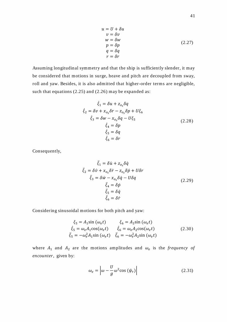
𝑢 = 𝑈 + 𝛿𝑢𝑣 = 𝛿𝑣𝑤 = 𝛿𝑤𝑝 = 𝛿𝑝𝑞 = 𝛿𝑞𝑟 = 𝛿𝑟

(2.27)

Assuming longitudinal symmetry and that the ship is sufficiently slender, it may

be considered that motions in surge, heave and pitch are decoupled from sway,

roll and yaw. Besides, it is also admitted that higher-order terms are negligible,

such that equations (2.25) and (2.26) may be expanded as:

�̇�1 = 𝛿𝑢 + 𝑧𝑜𝑠𝛿𝑞�̇�2 = 𝛿𝑣 + 𝑥𝑜𝑠𝛿𝑟 − 𝑧𝑜𝑠𝛿𝑝 + 𝑈𝜉6

�̇�3 = 𝛿𝑤 − 𝑥𝑜𝑠𝛿𝑞 − 𝑈𝜉5�̇�4 = 𝛿𝑝�̇�5 = 𝛿𝑞�̇�6 = 𝛿𝑟

(2.28)

Consequently,

�̈�1 = 𝛿�̇� + 𝑧𝑜𝑠𝛿�̇��̈�2 = 𝛿�̇� + 𝑥𝑜𝑠𝛿�̇� − 𝑧𝑜𝑠𝛿�̇� + 𝑈𝛿𝑟

�̈�3 = 𝛿�̇� − 𝑥𝑜𝑠𝛿�̇� − 𝑈𝛿𝑞�̈�4 = 𝛿�̇��̈�5 = 𝛿�̇��̈�6 = 𝛿�̇�

(2.29)

Considering sinusoidal motions for both pitch and yaw:

𝜉5 = 𝐴1sin (𝜔𝑒𝑡) 𝜉6 = 𝐴2sin (𝜔𝑒𝑡)�̇�5 = 𝜔𝑒𝐴1cos(𝜔𝑒𝑡) �̇�6 = 𝜔𝑒𝐴2cos(𝜔𝑒𝑡)�̈�5 = −𝜔𝑒2𝐴1sin (𝜔𝑒𝑡) �̈�6 = −𝜔𝑒2𝐴2sin (𝜔𝑒𝑡)

(2.30)

where 𝐴1 and 𝐴2 are the motions amplitudes and 𝜔𝑒 is the frequency of

encounter, given by:

𝜔𝑒 = �𝜔 −𝑈𝑔𝜔2cos (𝜓𝑟)� (2.31)

42

with 𝑔 being the acceleration of gravity and 𝜓𝑟 the relative wave incidence.

From (2.30), it is easy to notice that:

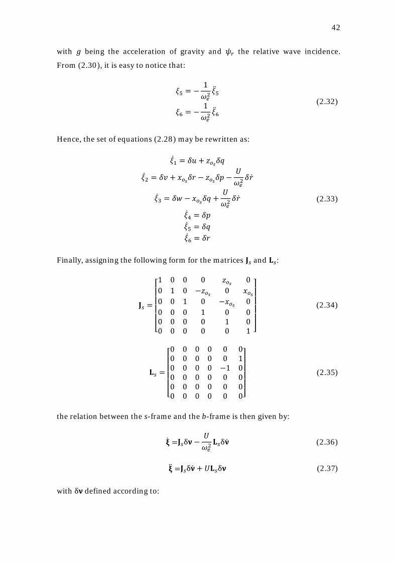
𝜉5 = −

1𝜔𝑒2

�̈�5

𝜉6 = −1𝜔𝑒2

�̈�6 (2.32)

Hence, the set of equations (2.28) may be rewritten as:

�̇�1 = 𝛿𝑢 + 𝑧𝑜𝑠𝛿𝑞

�̇�2 = 𝛿𝑣 + 𝑥𝑜𝑠𝛿𝑟 − 𝑧𝑜𝑠𝛿𝑝 −𝑈𝜔𝑒2

𝛿�̇�

�̇�3 = 𝛿𝑤 − 𝑥𝑜𝑠𝛿𝑞 +𝑈𝜔𝑒2

𝛿�̇�

�̇�4 = 𝛿𝑝�̇�5 = 𝛿𝑞�̇�6 = 𝛿𝑟

(2.33)

Finally, assigning the following form for the matrices 𝐉𝑠 and 𝐋𝑠:

𝐉𝑠 =

⎣⎢⎢⎢⎢⎡1 0 0 0 𝑧𝑜𝑠 00 1 0 −𝑧𝑜𝑠 0 𝑥𝑜𝑠0 0 1 0 −𝑥𝑜𝑠 00 0 0 1 0 00 0 0 0 1 00 0 0 0 0 1 ⎦

⎥⎥⎥⎥⎤

(2.34)

𝐋𝑠 =

⎣⎢⎢⎢⎢⎡0 0 0 0 0 00 0 0 0 0 10 0 0 0 −1 00 0 0 0 0 00 0 0 0 0 00 0 0 0 0 0⎦

⎥⎥⎥⎥⎤

(2.35)

the relation between the s-frame and the b-frame is then given by:

�̇� =𝐉𝑠δ𝛎 −𝑈𝜔𝑒2

𝐋𝑠δ�̇� (2.36)

�̈� =𝐉𝑠δ�̇� + 𝑈𝐋𝑠δ𝛎 (2.37)

with δ𝛎 defined according to:

43

δ𝛎 = [𝛿𝑢, 𝛿𝑣, 𝛿𝑤, 𝛿𝑝, 𝛿𝑞, 𝛿𝑟]T (2.38)

2.3.3 Transformation from b-frame to n-frame

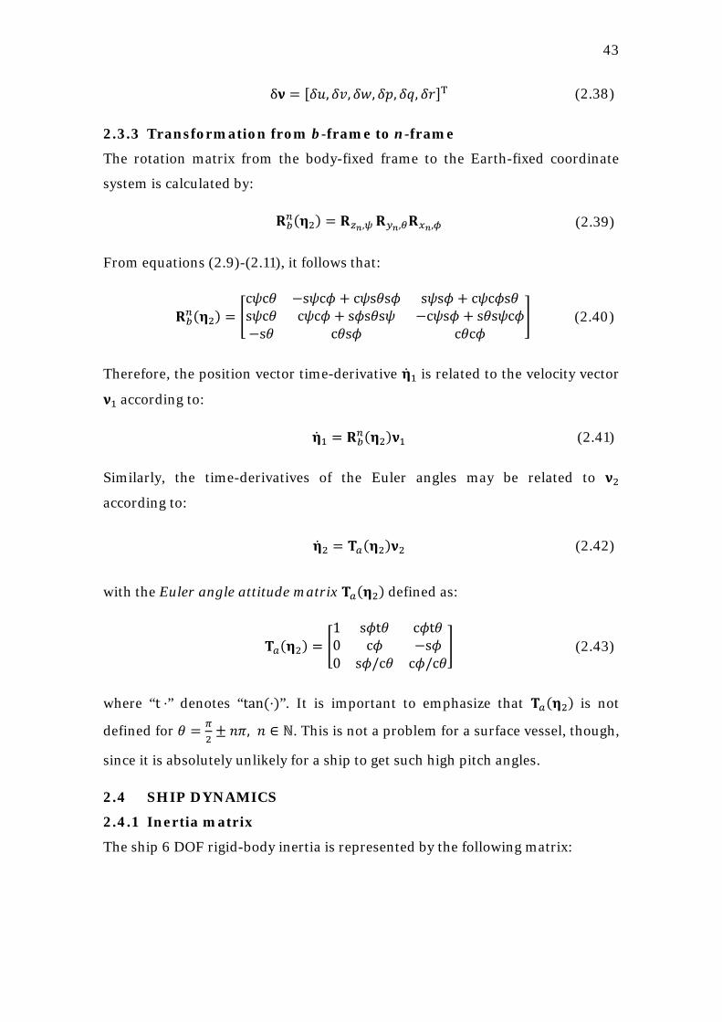
The rotation matrix from the body-fixed frame to the Earth-fixed coordinate

system is calculated by:

𝐑𝑏𝑛(𝛈2) = 𝐑𝑧𝑛,𝜓 𝐑𝑦𝑛,𝜃𝐑𝑥𝑛,𝜙 (2.39)

From equations (2.9)-(2.11), it follows that:

𝐑𝑏𝑛(𝛈2) = �

c𝜓c𝜃 −s𝜓c𝜙 + c𝜓s𝜃s𝜙 s𝜓s𝜙 + c𝜓c𝜙s𝜃s𝜓c𝜃 c𝜓c𝜙 + s𝜙s𝜃s𝜓 −c𝜓s𝜙 + s𝜃s𝜓c𝜙−s𝜃 c𝜃s𝜙 c𝜃c𝜙

� (2.40)

Therefore, the position vector time-derivative �̇�1 is related to the velocity vector

𝛎1 according to:

�̇�1 = 𝐑𝑏𝑛(𝛈2)𝛎1 (2.41)

Similarly, the time-derivatives of the Euler angles may be related to 𝛎2

according to:

�̇�2 = 𝐓𝑎(𝛈2)𝛎2 (2.42)

with the Euler angle attitude matrix 𝐓𝑎(𝛈2) defined as:

𝐓𝑎(𝛈2) = �1 s𝜙t𝜃 c𝜙t𝜃0 c𝜙 −s𝜙0 s𝜙/c𝜃 c𝜙/c𝜃

� (2.43)

where “t ⋅” denotes “tan(⋅)”. It is important to emphasize that 𝐓𝑎(𝛈2) is not

defined for 𝜃 = 𝜋2

± 𝑛𝜋, 𝑛 ∈ ℕ. This is not a problem for a surface vessel, though,

since it is absolutely unlikely for a ship to get such high pitch angles.

2.4 SHIP DYNAMICS

2.4.1 Inertia matrix

The ship 6 DOF rigid-body inertia is represented by the following matrix:

44

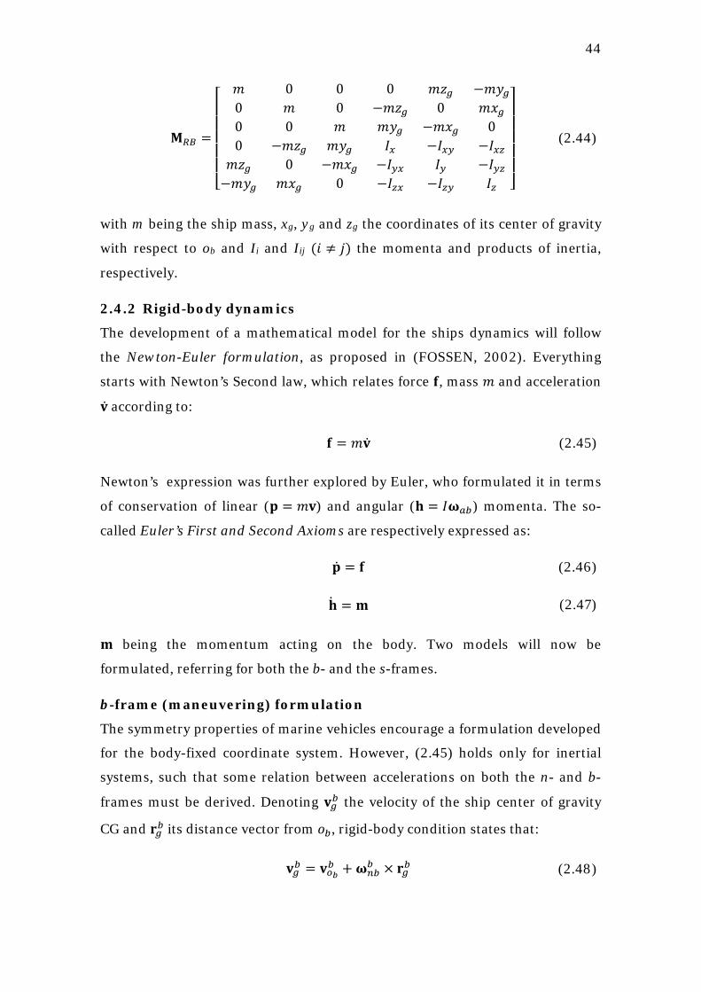
𝐌𝑅𝐵 =

⎣⎢⎢⎢⎢⎢⎡𝑚 0 0 0 𝑚𝑧𝑔 −𝑚𝑦𝑔0 𝑚 0 −𝑚𝑧𝑔 0 𝑚𝑥𝑔0 0 𝑚 𝑚𝑦𝑔 −𝑚𝑥𝑔 00 −𝑚𝑧𝑔 𝑚𝑦𝑔 𝐼𝑥 −𝐼𝑥𝑦 −𝐼𝑥𝑧𝑚𝑧𝑔 0 −𝑚𝑥𝑔 −𝐼𝑦𝑥 𝐼𝑦 −𝐼𝑦𝑧−𝑚𝑦𝑔 𝑚𝑥𝑔 0 −𝐼𝑧𝑥 −𝐼𝑧𝑦 𝐼𝑧 ⎦

⎥⎥⎥⎥⎥⎤

(2.44)

with m being the ship mass, xg, yg and zg the coordinates of its center of gravity

with respect to ob and Ii and Iij (𝑖 ≠ 𝑗) the momenta and products of inertia,

respectively.

2.4.2 Rigid-body dynamics

The development of a mathematical model for the ships dynamics will follow

the Newton-Euler formulation, as proposed in (FOSSEN, 2002). Everything

starts with Newton’s Second law, which relates force 𝐟, mass 𝑚 and acceleration

�̇� according to:

𝐟 = 𝑚�̇� (2.45)

Newton’s expression was further explored by Euler, who formulated it in terms

of conservation of linear (𝐩 = 𝑚𝐯) and angular (𝐡 = 𝐼𝛚𝑎𝑏) momenta. The so-

called Euler’s First and Second Axioms are respectively expressed as:

�̇� = 𝐟 (2.46)

�̇� = 𝐦 (2.47)

𝐦 being the momentum acting on the body. Two models will now be

formulated, referring for both the b- and the s-frames.

b-frame (maneuvering) formulation

The symmetry properties of marine vehicles encourage a formulation developed

for the body-fixed coordinate system. However, (2.45) holds only for inertial

systems, such that some relation between accelerations on both the n- and b-

frames must be derived. Denoting 𝐯𝑔𝑏 the velocity of the ship center of gravity

CG and 𝐫𝑔𝑏 its distance vector from 𝑜𝑏, rigid-body condition states that:

𝐯𝑔𝑏 = 𝐯𝑜𝑏𝑏 + 𝛚𝑛𝑏

𝑏 × 𝐫𝑔𝑏 (2.48)

45

where 𝛚𝑛𝑏𝑏 = 𝛎2. Therefore,

𝐯𝑔𝑛 = 𝐑𝑏𝑛𝐯𝑔𝑏 = 𝐑𝑏

𝑛�𝐯𝑜𝑏𝑏 + 𝛚𝑛𝑏

𝑏 × 𝐫𝑔𝑏� (2.49)

Time differentiating 𝐯𝑔𝑛 and substituting in Euler’s first axiom (2.46) yields:

𝑚��̇�𝑜𝑏𝑏 + 𝐒��̇�𝑛𝑏

𝑏 �𝐫𝑔𝑏 + 𝐒�𝛚𝑛𝑏𝑏 �𝐯𝑜𝑏

𝑏 + 𝐒𝟐�𝛚𝑛𝑏𝑏 �𝐫𝑔𝑏� = 𝐟𝑜𝑏 (2.50)

For the rotational motion, it is first necessary to write the expressions for the

angular momenta in 𝑜𝑏 and CG with respect to the b-frame, 𝐡𝑜𝑏𝑏 and 𝐡𝑔𝑏 :

𝐡𝑜𝑏𝑏 = 𝐈𝑜𝑏𝛚𝑛𝑏

𝑏 + 𝑚𝐫𝑔𝑏 × 𝐯𝑜𝑏𝑏 (2.51)

𝐡𝑔𝑏 = 𝐡𝑜𝑏𝑏 − 𝑚𝐫𝑔𝑏 × 𝐯𝑔𝑏 (2.52)

where 𝐈𝑜𝑏 is a partition from 𝐌𝑅𝐵:

𝐈𝑜𝑏 = �𝐼𝑥 −𝐼𝑥𝑦 −𝐼𝑥𝑧−𝐼𝑦𝑥 𝐼𝑦 −𝐼𝑦𝑧−𝐼𝑧𝑥 −𝐼𝑧𝑦 𝐼𝑧

� (2.53)

Differentiating (2.52) and applying Euler’s second axiom (2.47) yields:

𝐈𝑜𝑏�̇�𝑛𝑏𝑏 + 𝐒�𝛚𝑛𝑏

𝑏 �𝐈𝑜𝑏𝛚𝑛𝑏𝑏 + 𝑚𝐒�𝐫𝑔𝑏��̇�𝑜𝑏

𝑏 + 𝑚𝐒�𝐫𝑔𝑏�𝐒�𝛚𝑛𝑏𝑏 �𝐯𝑜𝑏

𝑏 = 𝐦𝑜𝑏 (2.54)

The total set of maneuvering 6 DOF equations of motion comes from (2.50) and

(2.54):

𝑚��̇� − 𝑣𝑟 + 𝑤𝑞 − 𝑥𝑔(𝑞2 + 𝑟2) + 𝑦𝑔(𝑝𝑞 − �̇�) + 𝑧𝑔(𝑝𝑟 + �̇�)� = 𝑋

𝑚��̇� − 𝑤𝑝 + 𝑢𝑟 − 𝑦𝑔(𝑟2 + 𝑝2) + 𝑧𝑔(𝑞𝑟 − �̇�) + 𝑧𝑔(𝑞𝑝 + �̇�)� = 𝑌

𝑚��̇� − 𝑢𝑞 + 𝑣𝑝 − 𝑧𝑔(𝑝2 + 𝑞2) + 𝑥𝑔(𝑟𝑝 − �̇�) + 𝑦𝑔(𝑟𝑞 + �̇�)� = 𝑍

𝐼𝑥�̇� + �𝐼𝑧 − 𝐼𝑦�𝑞𝑟 − (�̇� + 𝑝𝑞)𝐼𝑥𝑧 + (𝑟2 − 𝑞2)𝐼𝑦𝑧 + (𝑝𝑟 − �̇�)𝐼𝑥𝑦

+ 𝑚�𝑦𝑔(�̇� − 𝑢𝑞 + 𝑣𝑝) − 𝑧𝑔(�̇� − 𝑤𝑝 + 𝑢𝑟)� = 𝐾

𝐼𝑦�̇� + (𝐼𝑥 − 𝐼𝑧)𝑟𝑝 − (�̇� + 𝑞𝑟)𝐼𝑥𝑦 + (𝑝2 − 𝑟2)𝐼𝑧𝑥 + (𝑞𝑝 − �̇�)𝐼𝑦𝑧

+ 𝑚�𝑧𝑔(�̇� − 𝑣𝑟 + 𝑤𝑞) − 𝑥𝑔(�̇� − 𝑢𝑞 + 𝑣𝑝)� = 𝑀

𝐼𝑧�̇� + �𝐼𝑦 − 𝐼𝑥�𝑝𝑞 − (�̇� + 𝑟𝑝)𝐼𝑦𝑧 + (𝑞2 − 𝑝2)𝐼𝑥𝑦 + (𝑟𝑞 − �̇�)𝐼𝑧𝑥

+ 𝑚�𝑥𝑔(�̇� − 𝑤𝑝 + 𝑢𝑟) − 𝑦𝑔(�̇� − 𝑣𝑟 + 𝑤𝑞)� = 𝑁

(2.55)

46

A more compact representation for (2.55) may be obtained using the vectorial

formulation introduced in (FOSSEN, 1991):

𝐌𝑅𝐵�̇� + 𝐂𝑅𝐵(𝛎)𝛎 = 𝛕 (2.56)

with the Coriolis and centripetal matrix 𝐂𝑅𝐵(𝛎) = −𝐂𝑅𝐵T (𝛎) given by:

𝐂𝑅𝐵(𝛎) = �𝟎3X3 −𝑚𝐒(𝛎1) −𝑚𝐒(𝛎2)𝐒�𝐫𝑔𝑏�

−𝑚𝐒(𝛎1) + 𝑚𝐒�𝐫𝑔𝑏�𝐒(𝛎2) −𝐒(𝐈o𝛎2)� (2.57)

The generalized forces vector 𝛕 is composed by a parcel due to hydrodynamic

and hydrostatic loads 𝛕ℎ𝑦𝑑, an environment term 𝛕𝑒𝑛𝑣 and a control loads vector

𝛕𝑐𝑜𝑛, composed of forces/moments due to control, mooring, fenders and any

other positioning element. Hence:

𝛕 = 𝛕ℎ𝑦𝑑 + 𝛕𝑒𝑛𝑣 + 𝛕𝑐𝑜𝑛 (2.58)

s-frame (seakeeping) formulation

Once the seakeeping coordinate system moves with constant speed and

direction with respect to the Earth-fixed frame, it is also considered to be

inertial. Therefore, Newton’s Second Law may be directly applied:

𝐌𝑅𝐵,𝑠�̈� = 𝛿𝛕 (2.59)

Where 𝐌𝑅𝐵,𝑠 is the inertia matrix calculated in terms of the s-frame, related to

𝐌𝑅𝐵 according to:

𝐌𝑅𝐵 = 𝐉𝑠T𝐌𝑅𝐵,𝑠𝐉𝑠 (2.60)

Again, the generalized forces vector δ𝛕 is a superposition of hydrodynamic (and

hydrostatic), environmental and control loads:

𝛿𝛕 = 𝛿𝛕ℎ𝑦𝑑 + 𝛿𝛕𝑊𝐹 + 𝛿𝛕𝑐𝑜𝑛 (2.61)

Where 𝛿𝛕𝑊𝐹 corresponds to first-order wave loads, whose origin will be further

explained in section 2.6. Environmental action other than 1st order wave loads

are not in scope of seakeeping analysis.

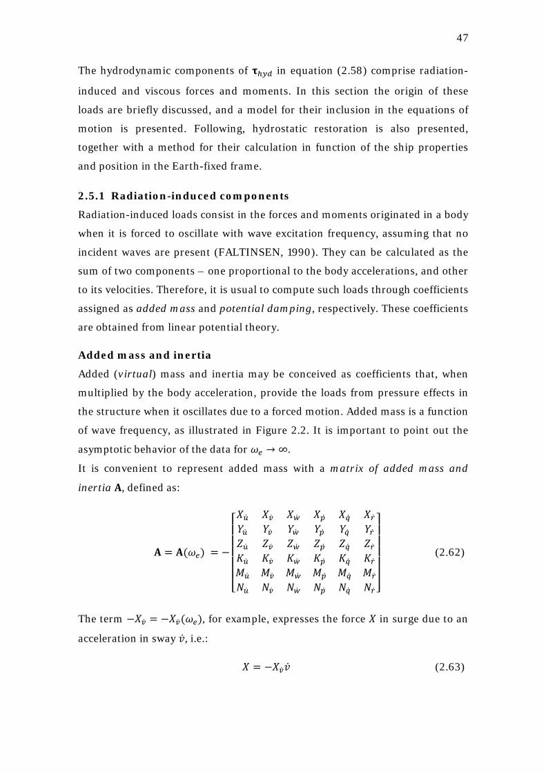
2.5 HYDRODYNAMICS AND HYDROSTATICS

47

The hydrodynamic components of 𝛕ℎ𝑦𝑑 in equation (2.58) comprise radiation-

induced and viscous forces and moments. In this section the origin of these

loads are briefly discussed, and a model for their inclusion in the equations of

motion is presented. Following, hydrostatic restoration is also presented,

together with a method for their calculation in function of the ship properties

and position in the Earth-fixed frame.

2.5.1 Radiation-induced components

Radiation-induced loads consist in the forces and moments originated in a body

when it is forced to oscillate with wave excitation frequency, assuming that no

incident waves are present (FALTINSEN, 1990). They can be calculated as the

sum of two components – one proportional to the body accelerations, and other

to its velocities. Therefore, it is usual to compute such loads through coefficients

assigned as added mass and potential damping, respectively. These coefficients

are obtained from linear potential theory.

Added mass and inertia

Added (virtual) mass and inertia may be conceived as coefficients that, when

multiplied by the body acceleration, provide the loads from pressure effects in

the structure when it oscillates due to a forced motion. Added mass is a function

of wave frequency, as illustrated in Figure 2.2. It is important to point out the

asymptotic behavior of the data for 𝜔𝑒 → ∞.

It is convenient to represent added mass with a matrix of added mass and

inertia 𝐀, defined as:

𝐀 = 𝐀(𝜔𝑒) = −

⎣⎢⎢⎢⎢⎢⎡𝑋�̇� 𝑋�̇� 𝑋�̇� 𝑋�̇� 𝑋�̇� 𝑋�̇�𝑌�̇� 𝑌�̇� 𝑌�̇� 𝑌�̇� 𝑌�̇� 𝑌�̇�𝑍�̇� 𝑍�̇� 𝑍�̇� 𝑍�̇� 𝑍�̇� 𝑍�̇�𝐾�̇� 𝐾�̇� 𝐾�̇� 𝐾�̇� 𝐾�̇� 𝐾�̇�𝑀�̇� 𝑀�̇� 𝑀�̇� 𝑀�̇� 𝑀�̇� 𝑀�̇�𝑁�̇� 𝑁�̇� 𝑁�̇� 𝑁�̇� 𝑁�̇� 𝑁�̇� ⎦

⎥⎥⎥⎥⎥⎤

(2.62)

The term −𝑋�̇� = −𝑋�̇�(𝜔𝑒), for example, expresses the force 𝑋 in surge due to an

acceleration in sway �̇�, i.e.:

𝑋 = −𝑋�̇��̇� (2.63)

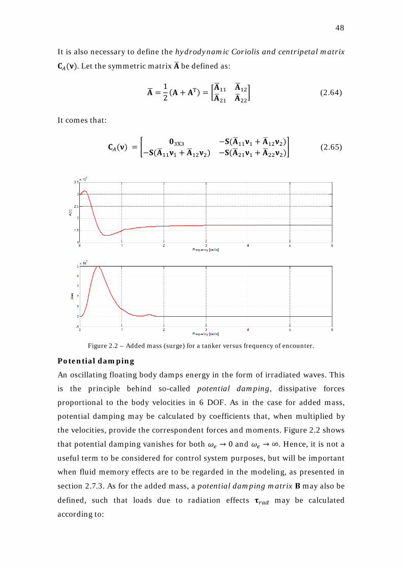
48

It is also necessary to define the hydrodynamic Coriolis and centripetal matrix

𝐂𝐴(𝛎). Let the symmetric matrix 𝐀� be defined as:

𝐀� =12

(𝐀 + 𝐀T) = �𝐀�11 𝐀�12𝐀�21 𝐀�22

� (2.64)

It comes that:

𝐂𝐴(𝛎) = �𝟎3X3 −𝐒(𝐀�11𝛎1 + 𝐀�12𝛎2)

−𝐒(𝐀�11𝛎1 + 𝐀�12𝛎2) −𝐒(𝐀�21𝛎1 + 𝐀�22𝛎2)� (2.65)

Figure 2.2 – Added mass (surge) for a tanker versus frequency of encounter.

Potential damping

An oscillating floating body damps energy in the form of irradiated waves. This

is the principle behind so-called potential damping, dissipative forces

proportional to the body velocities in 6 DOF. As in the case for added mass,

potential damping may be calculated by coefficients that, when multiplied by

the velocities, provide the correspondent forces and moments. Figure 2.2 shows

that potential damping vanishes for both 𝜔𝑒 → 0 and 𝜔𝑒 → ∞. Hence, it is not a

useful term to be considered for control system purposes, but will be important

when fluid memory effects are to be regarded in the modeling, as presented in

section 2.7.3. As for the added mass, a potential damping matrix 𝐁 may also be

defined, such that loads due to radiation effects 𝛕𝑟𝑎𝑑 may be calculated

according to:

49

𝛕𝑟𝑎𝑑 = 𝐀�̇� + 𝐁𝛎 + 𝐂𝐴(𝛎) 𝛎 (2.66)

Both added mass and potential damping coefficients may be obtained from

hydrodynamic software. These solvers may be based on both the panels-method

(like WAMIT and ANSYS AQWA) or on the strip theory (like VERES and

Octopus Seaway).

2.5.2 Viscous components

Viscous loads arise from viscid effects like skin friction and vortex shedding

(FOSSEN, 2002). Skin friction forces may be considered as the sum of both a

linear and a nonlinear component. The linear is based on laminar boundary

layer theory, being very important in the low-frequency motion of a body (and,

consequently, for the control system design). The nonlinear parcel originates

from the turbulent boundary layer, and corresponds to a high-frequency

contribution. Finally, by vortex-shedding one refers to the energy damped in

form of vortices originated from the ship motion.

As observed in (SKJETNE, SMOGELI and FOSSEN, 2004), the damping

component is the most uncertain among the parcels that compose the

hydrodynamic loads. Let the damping loads vector 𝐝(𝛎) be defined as:

𝐝(𝛎) = [𝑋𝑑(𝛎),𝑌𝑑(𝛎),𝑍𝑑(𝛎),𝐾𝑑(𝛎),𝑀𝑑(𝛎),𝑁𝑑(𝛎)]T (2.67)

It is convenient to assign 𝐝(𝛎) as a sum of linear and nonlinear components:

𝐝(𝛎) = 𝐃𝑙𝛎 + 𝐃𝑛(𝛎)𝛎 = 𝐃(𝛎)𝛎 (2.68)

The terms inside 𝐃𝑙 and 𝐃𝑛 may be calculated according to truncated Taylor

series expansions, as the widely used models proposed in (ABKOWITZ, 1964)

and (NORRBIN, 1970). A representation for 𝑌𝑑(𝛎) may be given, e.g., by:

𝑌𝑑(𝛎) = −𝑌𝑣𝑣 − 𝑌𝑟𝑟 − 𝑌|𝑣|𝑣|𝑣|𝑣 − 𝑌|𝑣|𝑟|𝑣|𝑟… (2.69)

where the coefficients 𝑌𝑣,𝑌|𝑣|𝑣, … may be obtained through PMM10

10 Planar motion mechanism.

model tests.

Some publications provide such coefficients, but they rarely relate to motions

other than surge, sway, yaw and, sometimes, roll.

50

2.5.3 Hydrostatic restoration

Restoration forces and moments arise from the balance between weight and

buoyancy, as stated by Archimedes’ principle. According to (FOSSEN, 2002),

the vector of restoration loads for box-shaped vessels 𝐠(𝛈) may be approximated

by a linear model, assuming yz-symmetry and small roll and pitch angles and

heave displacement:

𝐠(𝛈) ≈

⎣⎢⎢⎢⎢⎡

0 0

𝜌𝑤𝑔𝐴𝑤𝑝(0)𝑧𝜌𝑤𝑔∇𝐺𝑀��𝑇𝜙𝜌𝑤𝑔∇𝐺𝑀��𝐿𝜃

0 ⎦⎥⎥⎥⎥⎤

(2.70)

where 𝜌𝑤 is the water density, 𝐴𝑤𝑝(0) is the equilibrium water plane area,

∇= 𝑚/𝜌𝑤 is the volumetric displacement and 𝐺𝑀��𝑇 and 𝐺𝑀��𝐿 are the transversal

and longitudinal metacentric heights, respectively. This approximation

procedure is such that the vector 𝐠(𝛈) is already projected on the body-fixed

coordinate system. Let the restoration matrix 𝐆 be defined as:

𝐆 = −

⎣⎢⎢⎢⎢⎡0 0 0 0 0 00 0 0 0 0 00 0 𝜌𝑔𝐴𝑤𝑝(0) 0 0 00 0 0 𝜌𝑔∇ 𝐺𝑀��𝑇 0 00 0 0 0 𝜌𝑔∇ 𝐺𝑀��𝐿 00 0 0 0 0 0⎦

⎥⎥⎥⎥⎤

(2.71)

The vector 𝐠(𝛈) may then be calculated according to:

𝐠(𝛈) = 𝐆𝛈 (2.72)

Finally, the vector of hydrodynamic and hydrostatic forces and moments may be

defined:

𝛕ℎ𝑦𝑑 = −𝛕𝐚𝐝𝐝 − 𝐝(𝛎) − 𝐠(𝛈) = −𝐀�̇� − 𝐁𝛎 − 𝐂𝐴(𝛎) − 𝐃(𝛎)𝛎 − 𝐆𝛈 (2.73)

2.6 ENVIRONMENT MODELS

Environmental loads in ocean vehicles and structures originate from three main

agents, viz.

• Waves

51

• Wind

• Current

Thus, for simulation purposes it is necessary to adopt reliable models for both

describing such phenomena and estimating their loads in ships. This topic will

be approached in the present section.

2.6.1 Waves

Friction between wind and the ocean surface causes the appearance of small

perturbations in the water. Persistent wind action makes such perturbations to

grow until small waves begin to arise. These waves brake when they reach a

certain height, and their associated energy is damped. Therefore, when an ocean

storm begins a developing sea – characterized by short length 𝜆 waves – is

observed. Thus, the wave energy spectrum of a developing sea presents high-

frequency peak and narrow form. If the storm is long enough, a fully developed

sea takes place and the energy is distributed along wave components with

different associated frequencies. When the intense winds finally stop blowing,

the predominant frequency starts to decay, such that long waves – known as

swells – are then originated. From the dispersion relation for infinite water

depth, the wave velocity is given by (FALTINSEN, 1990):

𝑐 =𝜔𝑘

=𝑔𝜔

(2.74)

where 𝑘 = 2𝜋/𝜆 is the wave number. It may be concluded that low-frequency

swells have higher velocities, such that they propagate for longer distances and

may be observed very far from the place where they were originated.

The variation of wave elevation along the ship produces changes in the

distribution of the pressure field acting in the hull, inducing forces and

moments on it. Loads proportional to the wave height are called first order

wave loads and have the same frequency as the exciting waves. Components

proportional to the square of the wave height, on the other hand, are called

second order wave loads, which may be divided in slow drift (very small

frequency) and mean drift (zero frequency) forces.

1st order wave loads

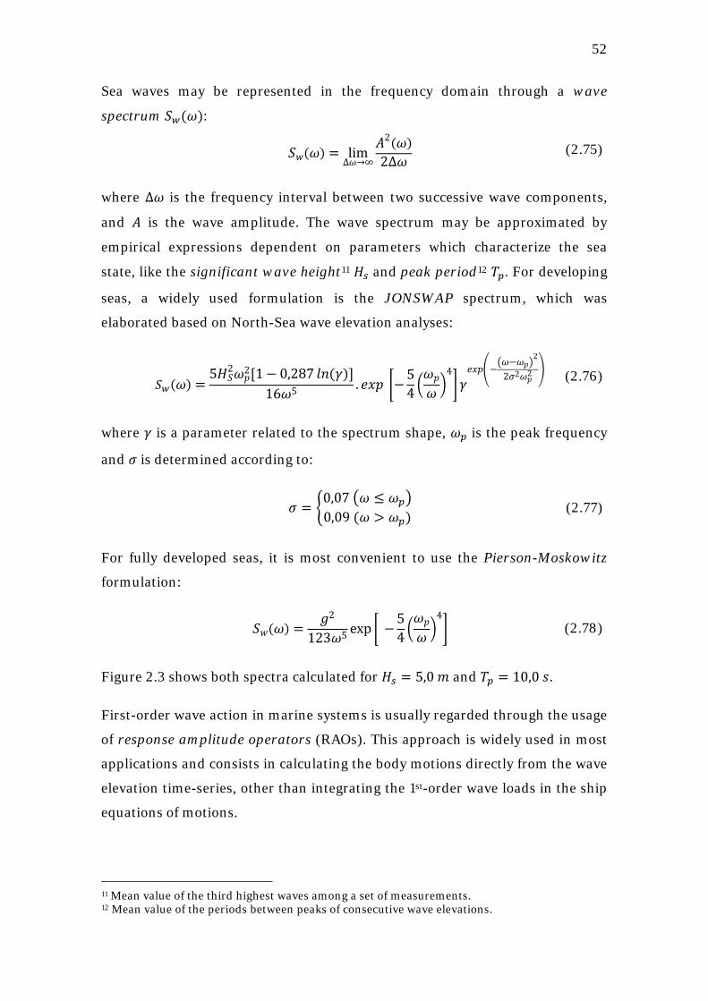
52

Sea waves may be represented in the frequency domain through a wave

spectrum 𝑆𝑤(𝜔):

𝑆𝑤(𝜔) = limΔ𝜔→∞

𝐴2(𝜔)2Δ𝜔 (2.75)

where ∆𝜔 is the frequency interval between two successive wave components,

and 𝐴 is the wave amplitude. The wave spectrum may be approximated by

empirical expressions dependent on parameters which characterize the sea

state, like the significant wave height11 𝐻𝑠 and peak period12

𝑇𝑝. For developing

seas, a widely used formulation is the JONSWAP spectrum, which was

elaborated based on North-Sea wave elevation analyses:

𝑆𝑤(𝜔) =5𝐻𝑆

2𝜔𝑝2[1− 0,287 𝑙𝑛(𝛾)]

16𝜔5 . 𝑒𝑥𝑝 �−54 �𝜔𝑝𝜔 �

4� 𝛾

𝑒𝑥𝑝�−�𝜔−𝜔𝑝�

2

2𝜎2𝜔𝑝2�

(2.76)

where 𝛾 is a parameter related to the spectrum shape, 𝜔𝑝 is the peak frequency

and 𝜎 is determined according to:

𝜎 = �0,07 �𝜔 ≤ 𝜔𝑝�0,09 (𝜔 > 𝜔𝑝)

� (2.77)

For fully developed seas, it is most convenient to use the Pierson-Moskowitz

formulation:

𝑆𝑤(𝜔) =𝑔2

123𝜔5 exp � −54 �𝜔𝑝𝜔 �

4� (2.78)

Figure 2.3 shows both spectra calculated for 𝐻𝑠 = 5,0 𝑚 and 𝑇𝑝 = 10,0 𝑠.

First-order wave action in marine systems is usually regarded through the usage

of response amplitude operators (RAOs). This approach is widely used in most

applications and consists in calculating the body motions directly from the wave

elevation time-series, other than integrating the 1st-order wave loads in the ship

equations of motions.

11 Mean value of the third highest waves among a set of measurements. 12 Mean value of the periods between peaks of consecutive wave elevations.

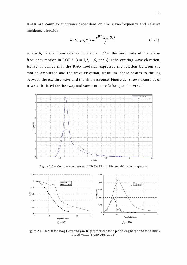
53

RAOs are complex functions dependent on the wave-frequency and relative

incidence direction:

𝑅𝐴𝑂𝑖(𝑗𝜔,𝛽𝑟) =𝑦𝑖𝑊𝐹(𝑗𝜔,𝛽𝑟)

𝜁 (2.79)

where 𝛽𝑟 is the wave relative incidence, 𝑦𝑖𝑊𝐹is the amplitude of the wave-

frequency motion in DOF i (𝑖 = 1,2, … ,6) and 𝜁 is the exciting wave elevation.

Hence, it comes that the RAO modulus expresses the relation between the

motion amplitude and the wave elevation, while the phase relates to the lag

between the exciting wave and the ship response. Figure 2.4 shows examples of

RAOs calculated for the sway and yaw motions of a barge and a VLCC.

Figure 2.3 – Comparison between JONSWAP and Pierson-Moskowitz spectra.

Figure 2.4 – RAOs for sway (left) and yaw (right) motions for a pipelaying barge and for a 100%

loaded VLCC (TANNURI, 2002).

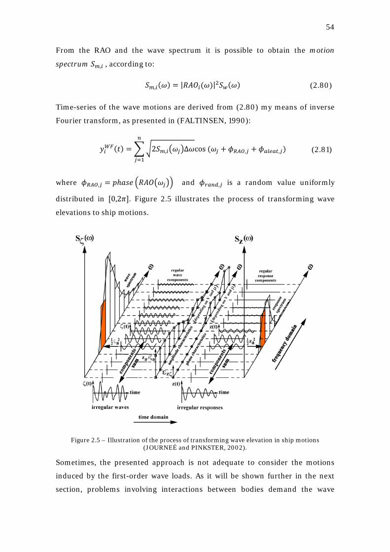
54

From the RAO and the wave spectrum it is possible to obtain the motion

spectrum 𝑆𝑚,𝑖 , according to:

𝑆𝑚,𝑖(𝜔) = |𝑅𝐴𝑂𝑖(𝜔)|2𝑆𝑤(𝜔) (2.80)

Time-series of the wave motions are derived from (2.80) my means of inverse

Fourier transform, as presented in (FALTINSEN, 1990):

𝑦𝑖𝑊𝐹(𝑡) = ��2𝑆𝑚,𝑖�𝜔𝑗�Δ𝜔cos (𝜔𝑗 + 𝜙𝑅𝐴𝑂,𝑗 + 𝜙𝑎𝑙𝑒𝑎𝑡,𝑗)𝑛

𝑗=1

(2.81)

where 𝜙𝑅𝐴𝑂,𝑗 = 𝑝ℎ𝑎𝑠𝑒 �𝑅𝐴𝑂�𝜔𝑗�� and 𝜙𝑟𝑎𝑛𝑑,𝑗 is a random value uniformly

distributed in [0,2𝜋]. Figure 2.5 illustrates the process of transforming wave

elevations to ship motions.

Figure 2.5 – Illustration of the process of transforming wave elevation in ship motions

(JOURNEÉ and PINKSTER, 2002).

Sometimes, the presented approach is not adequate to consider the motions

induced by the first-order wave loads. As it will be shown further in the next

section, problems involving interactions between bodies demand the wave

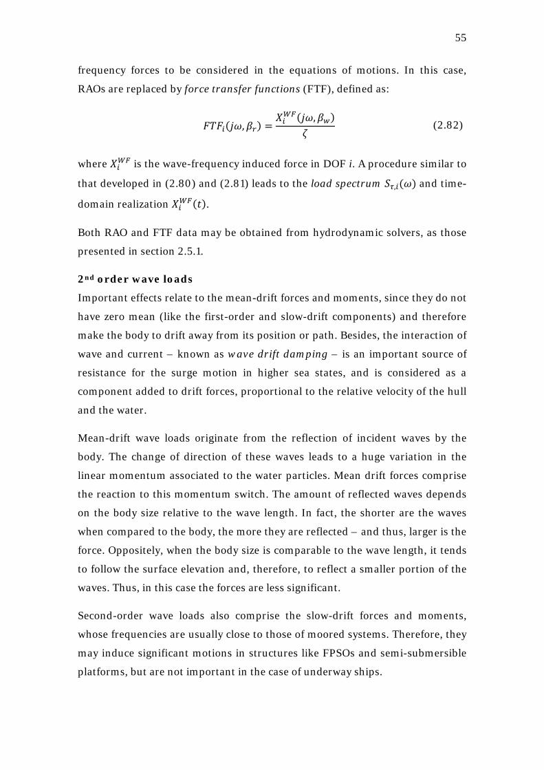
55

frequency forces to be considered in the equations of motions. In this case,

RAOs are replaced by force transfer functions (FTF), defined as:

𝐹𝑇𝐹𝑖(𝑗𝜔,𝛽𝑟) =𝑋𝑖𝑊𝐹(𝑗𝜔,𝛽𝑤)

𝜁 (2.82)

where 𝑋𝑖𝑊𝐹 is the wave-frequency induced force in DOF i. A procedure similar to

that developed in (2.80) and (2.81) leads to the load spectrum 𝑆𝜏,𝑖(𝜔) and time-

domain realization 𝑋𝑖𝑊𝐹(𝑡).

Both RAO and FTF data may be obtained from hydrodynamic solvers, as those

presented in section 2.5.1.

2nd order wave loads

Important effects relate to the mean-drift forces and moments, since they do not

have zero mean (like the first-order and slow-drift components) and therefore

make the body to drift away from its position or path. Besides, the interaction of

wave and current – known as wave drift damping – is an important source of

resistance for the surge motion in higher sea states, and is considered as a

component added to drift forces, proportional to the relative velocity of the hull

and the water.

Mean-drift wave loads originate from the reflection of incident waves by the

body. The change of direction of these waves leads to a huge variation in the

linear momentum associated to the water particles. Mean drift forces comprise

the reaction to this momentum switch. The amount of reflected waves depends

on the body size relative to the wave length. In fact, the shorter are the waves

when compared to the body, the more they are reflected – and thus, larger is the

force. Oppositely, when the body size is comparable to the wave length, it tends

to follow the surface elevation and, therefore, to reflect a smaller portion of the

waves. Thus, in this case the forces are less significant.

Second-order wave loads also comprise the slow-drift forces and moments,

whose frequencies are usually close to those of moored systems. Therefore, they

may induce significant motions in structures like FPSOs and semi-submersible

platforms, but are not important in the case of underway ships.

56

Calculation of mean-drift loads in irregular seas demands the use of drift

coefficients 𝐷(𝜔,𝛽𝑟), weighted by the wave spectrum. Such coefficients

correspond to the mean-drift forces evaluated for a given frequency and

incidence direction, normalized by the square of the wave amplitude. For the

scope of this work, only loads in surge, sway and yaw are of importance. The

generalized mean-drift forces are then calculated according to:

𝐹𝑖𝑀𝐷(𝑡) = 2� 𝑆(𝜔)𝐷𝑖(𝜔,𝛽𝑟)𝑑𝜔∞

0, 𝑖 = 1,2,6 (2.83)

Wave-drift damping evaluation will follow the procedure proposed in

(ARANHA, 1996), where the effect is regarded through alteration of the drift

coefficients. Let 𝑈𝑐𝑢𝑟𝑟 and 𝛼𝑟 be the current velocity (relative to the hull) and

relative incidence direction, respectively. The new coefficients are calculated

according to:

𝐷𝑤𝑑𝑑,𝑖(𝜔,𝛽𝑟) = 𝐷𝑖(𝜔,𝛽𝑟)

+𝑈𝑐𝑢𝑟𝑟𝑐

{cos(𝛼𝑟) [𝑏𝑤𝑖 cos(𝛽𝑟) + 𝑏𝑟𝑖 sin(𝛽𝑟)]

+ sin(𝛼𝑟) [𝑏𝑤𝑖 sin(𝛽𝑟) + 𝑏𝑟𝑖 cos(𝛽𝑟)]}

(2.84)

where the coefficients 𝑏𝑟𝑖 and 𝑏𝑤𝑖 are determined by:

𝑏𝑟𝑖 = −2𝜕𝐷𝑖(𝜔,𝛽𝑟)

𝜕𝛽𝑟 (2.85)

𝑏𝑤𝑖 = 4𝐷𝑖(𝜔,𝛽𝑟) + 𝜔𝜕𝐷𝑖(𝜔,𝛽𝑟)

𝜕𝜔 (2.86)

Then, in order to consider the wave-drift damping effect the original drift

coefficients 𝐷𝑖(𝜔,𝛽𝑟) in (2.83) must be replaced by the new coefficients

𝐷𝑤𝑑𝑑,𝑖(𝜔,𝛽𝑟) calculated in (2.84). (TANNURI, 2002) shows that for a static

VLCC under current of 1.2 m/s and 5.5 m height waves, with peak period of

11.4s, this correction may lead to a variation of 100% over the original value

(i.e., without wave-drift damping). It is important to emphasize, however, that

the formulation above was developed for a single body, and therefore is not

adequate for application on the side-by-side case.

2.6.2 Wind

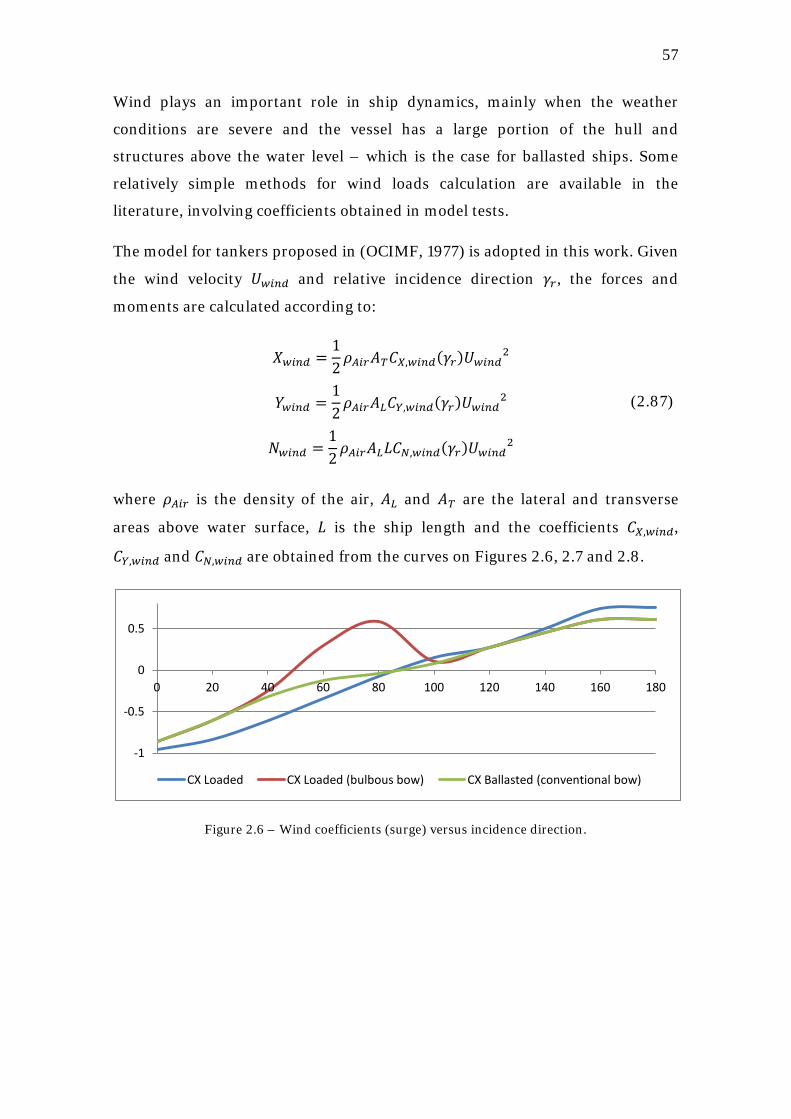
57

Wind plays an important role in ship dynamics, mainly when the weather

conditions are severe and the vessel has a large portion of the hull and

structures above the water level – which is the case for ballasted ships. Some

relatively simple methods for wind loads calculation are available in the

literature, involving coefficients obtained in model tests.

The model for tankers proposed in (OCIMF, 1977) is adopted in this work. Given

the wind velocity 𝑈𝑤𝑖𝑛𝑑 and relative incidence direction 𝛾𝑟, the forces and

moments are calculated according to:

𝑋𝑤𝑖𝑛𝑑 =12𝜌𝐴𝑖𝑟𝐴𝑇𝐶𝑋,𝑤𝑖𝑛𝑑(𝛾𝑟)𝑈𝑤𝑖𝑛𝑑2

𝑌𝑤𝑖𝑛𝑑 =12𝜌𝐴𝑖𝑟𝐴𝐿𝐶𝑌,𝑤𝑖𝑛𝑑(𝛾𝑟)𝑈𝑤𝑖𝑛𝑑2

𝑁𝑤𝑖𝑛𝑑 =12𝜌𝐴𝑖𝑟𝐴𝐿𝐿𝐶𝑁,𝑤𝑖𝑛𝑑(𝛾𝑟)𝑈𝑤𝑖𝑛𝑑2

(2.87)

where 𝜌𝐴𝑖𝑟 is the density of the air, 𝐴𝐿 and 𝐴𝑇 are the lateral and transverse

areas above water surface, 𝐿 is the ship length and the coefficients 𝐶𝑋,𝑤𝑖𝑛𝑑,

𝐶𝑌,𝑤𝑖𝑛𝑑 and 𝐶𝑁,𝑤𝑖𝑛𝑑 are obtained from the curves on Figures 2.6, 2.7 and 2.8.

Figure 2.6 – Wind coefficients (surge) versus incidence direction.

-1

-0.5

0

0.5

0 20 40 60 80 100 120 140 160 180

CX Loaded CX Loaded (bulbous bow) CX Ballasted (conventional bow)

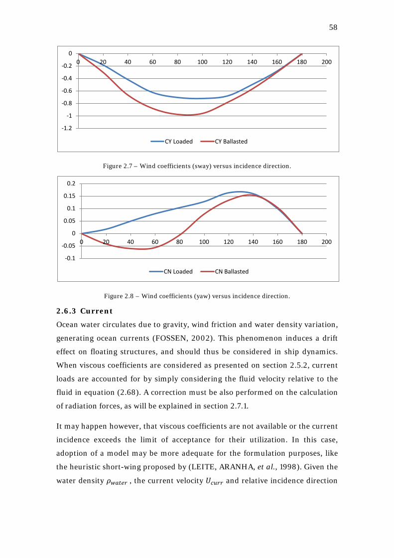
58

Figure 2.7 – Wind coefficients (sway) versus incidence direction.

Figure 2.8 – Wind coefficients (yaw) versus incidence direction.

2.6.3 Current

Ocean water circulates due to gravity, wind friction and water density variation,

generating ocean currents (FOSSEN, 2002). This phenomenon induces a drift

effect on floating structures, and should thus be considered in ship dynamics.

When viscous coefficients are considered as presented on section 2.5.2, current

loads are accounted for by simply considering the fluid velocity relative to the

fluid in equation (2.68). A correction must be also performed on the calculation

of radiation forces, as will be explained in section 2.7.1.

It may happen however, that viscous coefficients are not available or the current

incidence exceeds the limit of acceptance for their utilization. In this case,

adoption of a model may be more adequate for the formulation purposes, like

the heuristic short-wing proposed by (LEITE, ARANHA, et al., 1998). Given the

water density 𝜌𝑤𝑎𝑡𝑒𝑟 , the current velocity 𝑈𝑐𝑢𝑟𝑟 and relative incidence direction

-1.2

-1

-0.8

-0.6

-0.4

-0.2

0 0 20 40 60 80 100 120 140 160 180 200

CY Loaded CY Ballasted

-0.1

-0.05

0

0.05

0.1

0.15

0.2

0 20 40 60 80 100 120 140 160 180 200

CN Loaded CN Ballasted

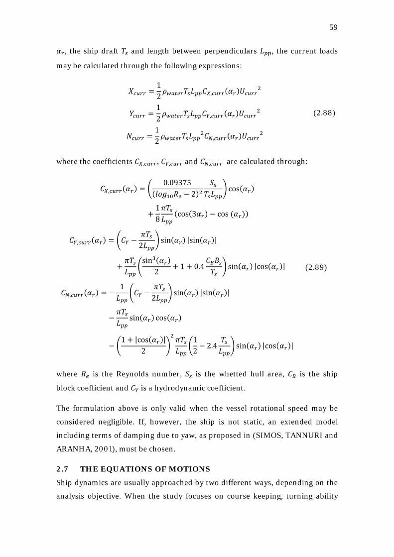
59

𝛼𝑟, the ship draft 𝑇𝑠 and length between perpendiculars 𝐿𝑝𝑝, the current loads

may be calculated through the following expressions:

𝑋𝑐𝑢𝑟𝑟 =12𝜌𝑤𝑎𝑡𝑒𝑟𝑇𝑠𝐿𝑝𝑝𝐶𝑋,𝑐𝑢𝑟𝑟(𝛼𝑟)𝑈𝑐𝑢𝑟𝑟2

𝑌𝑐𝑢𝑟𝑟 =12𝜌𝑤𝑎𝑡𝑒𝑟𝑇𝑠𝐿𝑝𝑝𝐶𝑌,𝑐𝑢𝑟𝑟(𝛼𝑟)𝑈𝑐𝑢𝑟𝑟2

𝑁𝑐𝑢𝑟𝑟 =12𝜌𝑤𝑎𝑡𝑒𝑟𝑇𝑠𝐿𝑝𝑝2𝐶𝑁,𝑐𝑢𝑟𝑟(𝛼𝑟)𝑈𝑐𝑢𝑟𝑟2

(2.88)

where the coefficients 𝐶𝑋,𝑐𝑢𝑟𝑟, 𝐶𝑌,𝑐𝑢𝑟𝑟 and 𝐶𝑁,𝑐𝑢𝑟𝑟 are calculated through:

𝐶𝑋,𝑐𝑢𝑟𝑟(𝛼𝑟) = �0.09375

(𝑙𝑜𝑔10𝑅𝑒 − 2)2𝑆𝑠

𝑇𝑠𝐿𝑝𝑝� cos(𝛼𝑟)

+18𝜋𝑇𝑠𝐿𝑝𝑝

(cos(3𝛼𝑟) − cos (𝛼𝑟))

𝐶𝑌,𝑐𝑢𝑟𝑟(𝛼𝑟) = �𝐶𝑌 −𝜋𝑇𝑠

2𝐿𝑝𝑝� sin(𝛼𝑟) |sin(𝛼𝑟)|

+𝜋𝑇𝑠𝐿𝑝𝑝

�sin3(𝛼𝑟)

2+ 1 + 0.4

𝐶𝐵𝐵𝑠𝑇𝑠

� sin(𝛼𝑟) |cos(𝛼𝑟)|

𝐶𝑁,𝑐𝑢𝑟𝑟(𝛼𝑟) = −1𝐿𝑝𝑝

�𝐶𝑌 −𝜋𝑇𝑠

2𝐿𝑝𝑝� sin(𝛼𝑟) |sin(𝛼𝑟)|

−𝜋𝑇𝑠𝐿𝑝𝑝

sin(𝛼𝑟) cos(𝛼𝑟)

− �1 + |cos(𝛼𝑟)|

2�2 𝜋𝑇𝑠𝐿𝑝𝑝

�12− 2.4

𝑇𝑠𝐿𝑝𝑝

� sin(𝛼𝑟) |cos(𝛼𝑟)|

(2.89)

where 𝑅𝑒 is the Reynolds number, 𝑆𝑠 is the whetted hull area, 𝐶𝐵 is the ship

block coefficient and 𝐶𝑌 is a hydrodynamic coefficient.

The formulation above is only valid when the vessel rotational speed may be

considered negligible. If, however, the ship is not static, an extended model

including terms of damping due to yaw, as proposed in (SIMOS, TANNURI and

ARANHA, 2001), must be chosen.

2.7 THE EQUATIONS OF MOTIONS

Ship dynamics are usually approached by two different ways, depending on the

analysis objective. When the study focuses on course keeping, turning ability

60

and controllability – in calm water – it is referred to as maneuvering. If, on the

other hand, one aims on the motions of a ship subjected to waves while moving

with constant speed and heading, the analysis is known as seakeeping. Usually,

the outcomes of both models are superposed for control systems design

purposes.

Some situations, however, demand a combination of both maneuvering and

seakeeping models (PEREZ, FOSSEN and SøRENSEN, 2004). Therefore, a

unified model will be presented based on the formulation proposed in

(FOSSEN, 2005). Such approach is necessary for the case, e.g., of two ships

advancing in waves with interaction forces (e.g. mooring loads), where the

division of the problem as stated above is inadequate.

2.7.1 Maneuvering

In the study of maneuvering, it is admitted that no first-order motions due to

waves affect the ship. Therefore, the hydrodynamic coefficients correspond to

the zero-frequency asymptotic values, i.e.:

𝐀 = 𝐀(0) = 𝐀0 (2.90)

𝐁 = 𝐁(0) = 𝟎6𝑋6 (2.91)

Such that equation (2.73) reduces to:

𝛕ℎ𝑦𝑑 = −𝐀0�̇� − 𝐂𝐴0(𝛎) − 𝐃(𝛎)𝛎 − 𝐆𝛈 (2.92)

Replacing 𝛕ℎ𝑦𝑑 in (2.58) by the above expression and then substituting the

result in (2.56) yields:

(𝐌𝑅𝐵 + 𝐀0)�̇� + [𝐂𝑅𝐵(𝛎) + 𝐂𝐴0(𝛎)]𝛎 + 𝐃(𝛎)𝛎 + 𝐆𝛈 = 𝛕𝑒𝑛𝑣 + 𝛕𝑐𝑜𝑛 (2.93)

The velocity vector 𝛎 may not be directly integrated in time in order to get the

positions and orientation angles. The coordinates transformation from b- to n-

frame is performed through (2.41) and (2.42), in order to obtain the vector �̇�.

Let 𝐉𝐛𝐧(𝛎) be defined as:

𝐉𝐛𝐧(𝛈𝟐) = �𝐑𝑏𝑛(𝛈2) 𝟎3𝑋3𝟎3𝑋3 𝐓𝑎(𝛈2)� (2.94)

Such that the relation below holds:

61

�̇� = 𝐉𝑏𝑛(𝛈𝟐)𝛎 (2.95)

The formulation above does not consider the effect of ocean currents. In fact,

current makes the absolute velocity vector 𝛎 to be different from the velocity of

the water relative to the hull. Let the current velocity vector 𝛎c, correspondent

to the components of the current in the 𝑥𝑏 and 𝑦𝑏 axes, be defined as:

𝛎𝑐 =

⎣⎢⎢⎢⎢⎡𝑈𝑐𝑢𝑟𝑟cos (𝛼𝑟)𝑈𝑐𝑢𝑟𝑟 sin(𝛼𝑟)

0000 ⎦

⎥⎥⎥⎥⎤

(2.96)

The relative velocity vector 𝛎𝑟 is obtained according to:

𝛎𝑟 = 𝛎 − 𝛎c =

⎣⎢⎢⎢⎢⎡𝑢𝑟𝑣𝑟𝑧𝑝𝑞𝑟 ⎦⎥⎥⎥⎥⎤

(2.97)

Radiation loads depend on the relative velocity, since they are related to the

pressure exerted by the water in the ship hull. Therefore, 𝛕ℎ𝑦𝑑 in (2.92) must be

calculated in terms of 𝛎𝑟, i.e. (SKJETNE, SMOGELI and FOSSEN, 2004):

𝛕ℎ𝑦𝑑 = −𝐀0�̇�𝑟 − 𝐂𝐴0(𝛎𝑟) − 𝐃(𝛎𝑟)𝛎𝑟 − 𝐆𝛈 (2.98)

From the definition of the first two elements 𝑢𝑐 and 𝑣𝑐 of vector 𝛎𝑐 (as defined in

(2.98)), it may be easily deduced that their time-derivatives may be calculated

as:

�̇�𝑐 = 𝑟𝑣𝑐

�̇�𝑐 = −𝑟𝑢𝑐 (2.99)

Such that �̇�𝑟 is obtained through:

�̇�𝑟 = �̇� − �̇�c =

⎣⎢⎢⎢⎢⎡�̇� − 𝑟𝑣𝑐�̇� + 𝑟𝑢𝑐

�̇��̇��̇��̇� ⎦

⎥⎥⎥⎥⎤

(2.100)

62

Finally, equation (2.93) may be rewritten, considering the relative velocity

effects:

𝐌𝑅𝐵�̇� + 𝐀0�̇�𝑟 + 𝐂𝑅𝐵(𝛎)𝛎 + 𝐂𝐴0(𝛎𝑟)𝛎𝑟 + 𝐃(𝛎𝑟)𝛎𝑟 + 𝐆𝛈

= 𝛕𝑒𝑛𝑣 + 𝛕𝑐𝑜𝑛 (2.101)

The equations of motion in 6 DOF are only meaningful when vertical (heave,

roll and pitch) motions are to be considered in the model. This is usually the

case when the relative motions of two bodies close from each other are to be

analyzed. However, most of the cases in maneuvering concern only to horizontal

(surge, sway and yaw) motions. Especially for marine control design, the

equations of motions in 3 DOF are more likely to be utilized than the complete

formulation presented above. Let the subscript ℎ indicate the horizontal

motions. The position 𝛈ℎ and velocity 𝛎ℎ vectors are defined as:

𝛈ℎ = [𝑥,𝑦,𝜓]T

𝛎ℎ = [𝑢, 𝑣, 𝑟]T (2.102)

The matrices for 3 DOF are composed of the correspondent terms from 𝐌𝑅𝐵, 𝐀0,

𝐂𝑅𝐵(𝛎), 𝐂𝐴0(𝛎𝑟), 𝐃(𝛎𝑟) and 𝐆.

2.7.2 Seakeeping

Following the same approach used for maneuvering, seakeeping equations of

motion are formulated departing from the rigid-body dynamics results of

section 2.4.2. Once only the effect of first-order wave loads is to be considered,

the hydrodynamic (plus hydrostatic) term 𝛿𝛕ℎ𝑦𝑑 depends only on the radiation

and restoration forces:

𝛿𝛕ℎ𝑦𝑑 = −𝐀𝑠(𝜔𝑒)�̈� − 𝐁𝑠(𝜔𝑒)�̇� − 𝐆𝑠𝛏 (2.103)

where the subscript 𝑠 states that the matrices are computed for the seakeeping

coordinate system. It is worth to point out the dependence on the encounter

frequency for both the added mass and potential damping. From (2.59), (2.61)

and (2.103) it comes that:

�𝐌𝑅𝐵,𝑠 + 𝐀𝑠(𝜔𝑒)��̈�+ 𝐁𝑠(𝜔𝑒)�̇� + 𝐆𝑠𝛏 = 𝛿𝛕𝑊𝐹 + 𝛿𝛕𝑐𝑜𝑛 (2.104)

63

The term 𝛿𝛕𝑊𝐹 may be obtained from the wave elevation and the FTF, as

explained in section 2.6. Hydrodynamic solvers calculate both RAOs and FTFs

from equation (2.104), disregarding the control term 𝛿𝛕𝑐𝑜𝑛. For a discrete range

of encounter frequencies 𝜔𝑒, 𝛿𝛕𝑊𝐹 is admitted as a sinusoidal wave excitation,

and from the calculated response it is possible to obtain the desired transfer

function.

The formulation above is developed for the s-frame. To derive the same results

for the b-frame, (2.36) and (2.37) are substituted in (2.104) and both sides of

the resultant equation are multiplied by 𝐉𝑠T:

𝐉𝑠T�𝐌𝑅𝐵,𝑠 + 𝐀𝑠(𝜔𝑒)�(𝐉𝑠δ�̇� + 𝑈𝐋𝑠δ𝛎) + 𝐉𝑠T𝐁𝑠(𝜔𝑒) �𝐉𝑠δ𝛎 −

𝑈𝜔𝑒2

𝐋𝑠δ�̇��

+ 𝐉𝑠T𝐆𝑠𝛏 = 𝐉𝑠T(𝛿𝛕𝑊𝐹 + 𝛿𝛕𝑐𝑜𝑛) (2.105)

Using relation (2.60) and making the following substitutions:

𝐀�(ωe) = 𝐉𝑠T𝐀𝑠(𝜔𝑒)𝐉𝑠 −𝑈𝜔𝑒2

𝐉𝑠T𝐁𝑠(𝜔𝑒)𝐋𝑠

𝐃�(𝜔𝑒) = 𝐉𝑠T𝐁𝑠(𝜔𝑒)𝐉𝑠

𝐂𝑅𝐵 = 𝑈𝐉𝑠T𝐌𝑅𝐵,𝑠𝐋𝑠

𝐂�𝐴(𝜔𝑒) = 𝑈𝐉𝑠T𝐀𝑠(𝜔𝑒)𝐋𝑠

𝐍�(𝜔𝑒) = 𝐂�𝐴(𝜔𝑒) + 𝐃�(𝜔𝑒)

𝐆 = 𝐉𝑠T𝐆𝑠

𝛕𝑊𝐹 = 𝐉𝑠T𝛿𝛕𝑊𝐹

𝛕𝑐𝑜𝑛 − 𝛕�𝑐𝑜𝑛= 𝐉𝑠T𝛿𝛕𝑐𝑜𝑛

(2.106)

where 𝛕�𝑐𝑜𝑛 is the necessary control load for the ship to advance with velocity 𝑈,

it finally comes (FOSSEN, 2005):

�𝐌𝑅𝐵 + 𝐀�(𝜔𝑒)�𝛿�̇� + 𝐂𝑅𝐵𝛿𝛎 + 𝐍�(𝜔𝑒)𝛿𝛎 + 𝐆𝛏 = 𝛕𝑊𝐹 + (𝛕𝑐𝑜𝑛 − 𝛕�𝑐𝑜𝑛) (2.107)

Equations of motions for pure maneuvering and seakeeping have already been

presented. Now, a unified model for both approaches will be presented, based

on time-domain transformation of equation (2.107).

2.7.3 Unified model for maneuvering and seakeeping

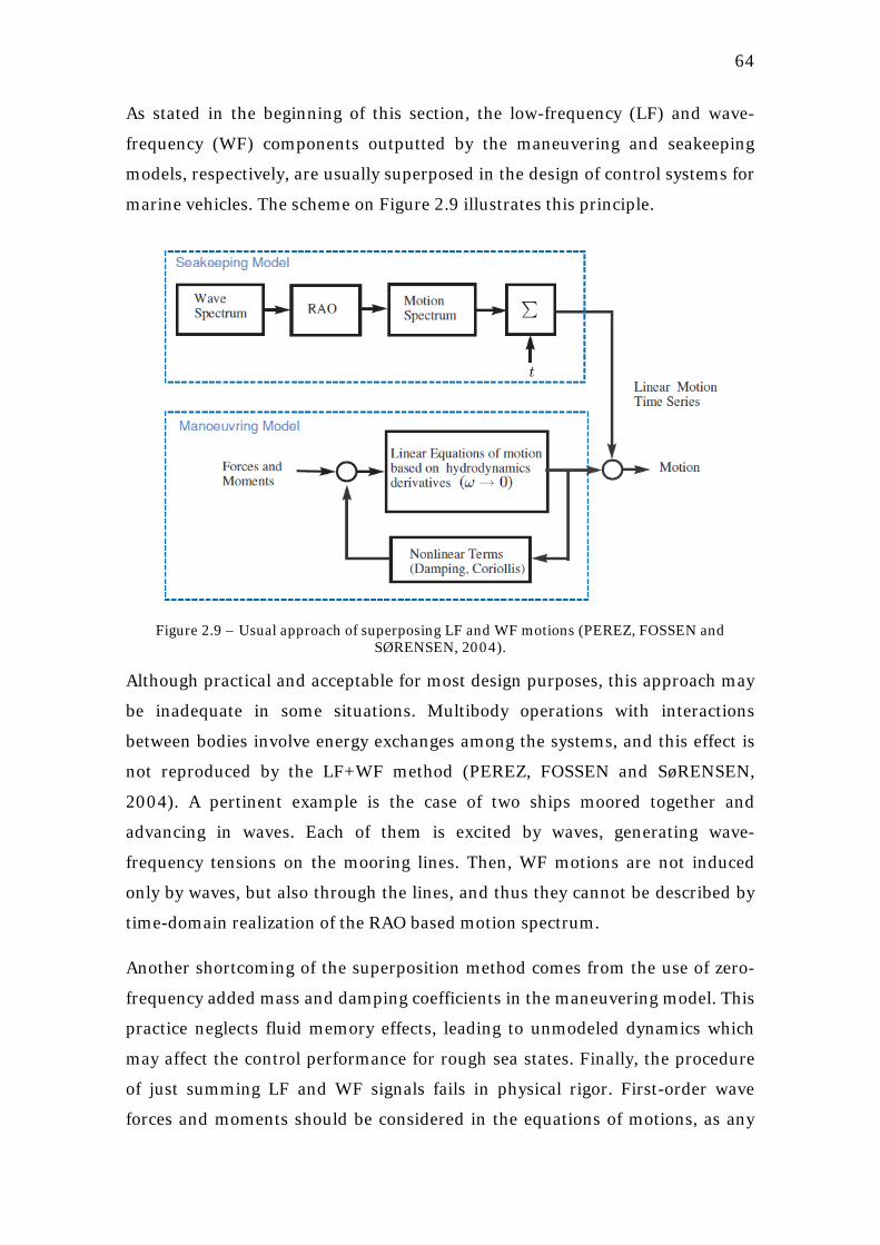
64

As stated in the beginning of this section, the low-frequency (LF) and wave-

frequency (WF) components outputted by the maneuvering and seakeeping

models, respectively, are usually superposed in the design of control systems for

marine vehicles. The scheme on Figure 2.9 illustrates this principle.

Figure 2.9 – Usual approach of superposing LF and WF motions (PEREZ, FOSSEN and

SØRENSEN, 2004).

Although practical and acceptable for most design purposes, this approach may

be inadequate in some situations. Multibody operations with interactions

between bodies involve energy exchanges among the systems, and this effect is

not reproduced by the LF+WF method (PEREZ, FOSSEN and SøRENSEN,

2004). A pertinent example is the case of two ships moored together and

advancing in waves. Each of them is excited by waves, generating wave-

frequency tensions on the mooring lines. Then, WF motions are not induced

only by waves, but also through the lines, and thus they cannot be described by

time-domain realization of the RAO based motion spectrum.

Another shortcoming of the superposition method comes from the use of zero-

frequency added mass and damping coefficients in the maneuvering model. This

practice neglects fluid memory effects, leading to unmodeled dynamics which

may affect the control performance for rough sea states. Finally, the procedure

of just summing LF and WF signals fails in physical rigor. First-order wave

forces and moments should be considered in the equations of motions, as any

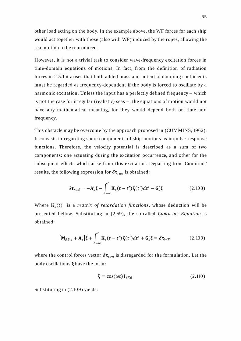
65

other load acting on the body. In the example above, the WF forces for each ship

would act together with those (also with WF) induced by the ropes, allowing the

real motion to be reproduced.

However, it is not a trivial task to consider wave-frequency excitation forces in

time-domain equations of motions. In fact, from the definition of radiation

forces in 2.5.1 it arises that both added mass and potential damping coefficients

must be regarded as frequency-dependent if the body is forced to oscillate by a

harmonic excitation. Unless the input has a perfectly defined frequency – which

is not the case for irregular (realistic) seas –, the equations of motion would not

have any mathematical meaning, for they would depend both on time and

frequency.

This obstacle may be overcome by the approach proposed in (CUMMINS, 1962).

It consists in regarding some components of ship motions as impulse-response

functions. Therefore, the velocity potential is described as a sum of two

components: one actuating during the excitation occurrence, and other for the

subsequent effects which arise from this excitation. Departing from Cummins’

results, the following expression for 𝛿𝛕𝑟𝑎𝑑 is obtained:

𝛿𝛕𝑟𝑎𝑑 = −𝐀𝑠′ �̈� − � 𝐊𝑠(𝑡 − 𝑡′)

𝑡

−∞�̇�(𝑡′)𝑑𝑡′ − 𝐆𝑠′ 𝛏 (2.108)

Where 𝐊𝑠(𝑡) is a matrix of retardation functions, whose deduction will be

presented bellow. Substituting in (2.59), the so-called Cummins Equation is

obtained:

�𝐌𝑅𝐵,𝑠 + 𝐀𝑠′ ��̈� + � 𝐊𝑠(𝑡 − 𝑡′)

𝑡

−∞�̇�(𝑡′)𝑑𝑡′ + 𝐆𝑠′ 𝛏 = 𝛿𝛕𝑊𝐹 (2.109)

where the control forces vector 𝛿𝛕𝑐𝑜𝑛 is disregarded for the formulation. Let the

body oscillations 𝛏 have the form:

𝛏 = cos(𝜔𝑡) 𝐈6𝑋6 (2.110)

Substituting in (2.109) yields:

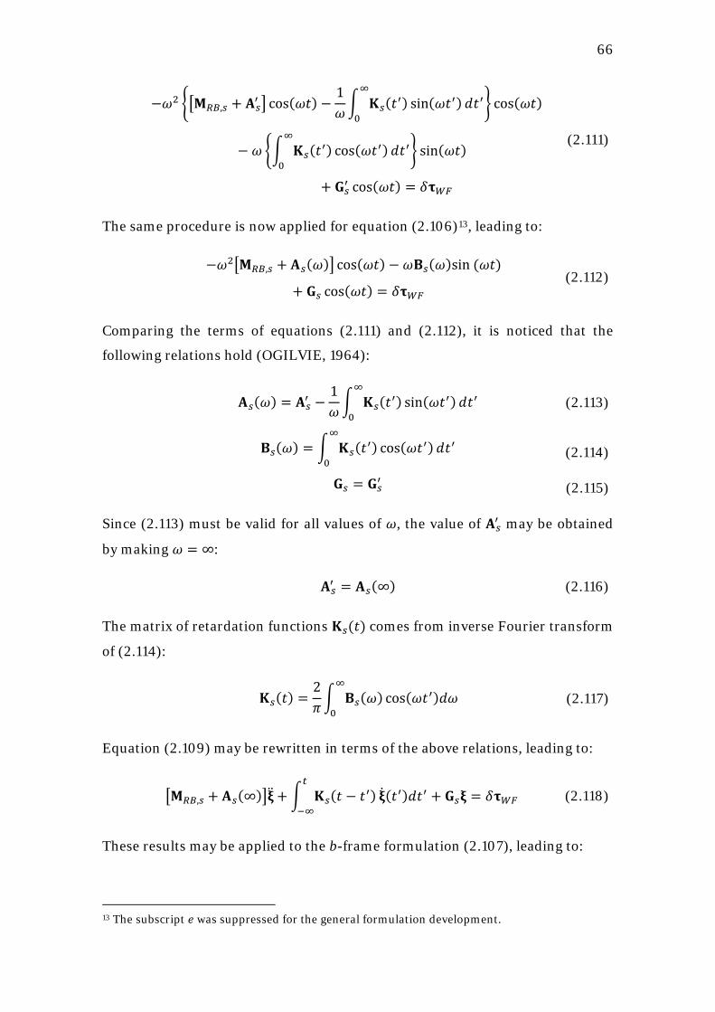
66

−𝜔2 ��𝐌𝑅𝐵,𝑠 + 𝐀𝑠′ � cos(𝜔𝑡) −

1𝜔� 𝐊𝑠(𝑡′)∞

0sin(𝜔𝑡′)𝑑𝑡′� cos(𝜔𝑡)

− 𝜔�� 𝐊𝑠(𝑡′)∞

0cos(𝜔𝑡′)𝑑𝑡′� sin(𝜔𝑡)

+ 𝐆𝑠′ cos(𝜔𝑡) = 𝛿𝛕𝑊𝐹

(2.111)

The same procedure is now applied for equation (2.106)13

, leading to:

−𝜔2�𝐌𝑅𝐵,𝑠 + 𝐀𝑠(𝜔)� cos(𝜔𝑡) − 𝜔𝐁𝑠(𝜔)sin (𝜔𝑡)

+ 𝐆𝑠 cos(𝜔𝑡) = 𝛿𝛕𝑊𝐹 (2.112)

Comparing the terms of equations (2.111) and (2.112), it is noticed that the

following relations hold (OGILVIE, 1964):

𝐀𝑠(𝜔) = 𝐀𝑠′ −

1𝜔� 𝐊𝑠(𝑡′)∞

0sin(𝜔𝑡′)𝑑𝑡′ (2.113)

𝐁𝑠(𝜔) = � 𝐊𝑠(𝑡′)∞

0cos(𝜔𝑡′)𝑑𝑡′ (2.114)

𝐆𝑠 = 𝐆𝑠′ (2.115)

Since (2.113) must be valid for all values of 𝜔, the value of 𝐀𝑠′ may be obtained

by making 𝜔 = ∞:

𝐀𝑠′ = 𝐀𝑠(∞) (2.116)

The matrix of retardation functions 𝐊𝑠(𝑡) comes from inverse Fourier transform

of (2.114):

𝐊𝑠(𝑡) =2𝜋� 𝐁𝑠(𝜔)∞

0cos(𝜔𝑡′)𝑑𝜔 (2.117)

Equation (2.109) may be rewritten in terms of the above relations, leading to:

�𝐌𝑅𝐵,𝑠 + 𝐀𝑠(∞)��̈�+ � 𝐊𝑠(𝑡 − 𝑡′)𝑡

−∞�̇�(𝑡′)𝑑𝑡′ + 𝐆𝑠𝛏 = 𝛿𝛕𝑊𝐹 (2.118)

These results may be applied to the b-frame formulation (2.107), leading to:

13 The subscript 𝑒 was suppressed for the general formulation development.

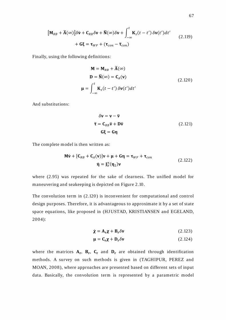
67

�𝐌𝑅𝐵 + 𝐀�(∞)�𝛿�̇� + 𝐂𝑅𝐵𝛿𝛎 + 𝐍�(∞)𝛿𝛎 + � 𝐊𝑠(𝑡 − 𝑡′)

𝑡

−∞𝛿𝛎(𝑡′)𝑑𝑡′

+ 𝐆𝛏 = 𝛕𝑊𝐹 + (𝛕𝑐𝑜𝑛 − 𝛕�𝑐𝑜𝑛) (2.119)

Finally, using the following definitions:

𝐌 = 𝐌𝑅𝐵 + 𝐀�(∞)

𝐃 = 𝐍�(∞) = 𝐂𝐴(𝛎)

𝛍 = � 𝐊𝑠(𝑡 − 𝑡′)𝑡

−∞𝛿𝛎(𝑡′)𝑑𝑡′

(2.120)

And substitutions:

𝛿𝛎 = 𝛎 − 𝛎�

𝛕� = 𝐂𝑅𝐵𝛎� + 𝐃𝛎�

𝐆𝛏 = 𝐆𝛈

(2.121)

The complete model is then written as:

𝐌�̇� + [𝐂𝑅𝐵 + 𝐂𝐴(𝛎)]𝛎 + 𝛍 + 𝐆𝛈 = 𝛕𝑊𝐹 + 𝛕𝑐𝑜𝑛

�̇� = 𝐉𝑏𝑛(𝛈2)𝛎 (2.122)

where (2.95) was repeated for the sake of clearness. The unified model for

maneuvering and seakeeping is depicted on Figure 2.10.

The convolution term in (2.120) is inconvenient for computational and control

design purposes. Therefore, it is advantageous to approximate it by a set of state

space equations, like proposed in (HJUSTAD, KRISTIANSEN and EGELAND,

2004):

�̇� = 𝐀𝐫𝛘 + 𝐁𝐫𝛿𝛎 (2.123)

𝛍 = 𝐂𝐫𝛘 + 𝐃𝐫𝛿𝛎 (2.124)

where the matrices 𝐀𝐫, 𝐁𝐫, 𝐂𝐫 and 𝐃𝐫 are obtained through identification

methods. A survey on such methods is given in (TAGHIPUR, PEREZ and

MOAN, 2008), where approaches are presented based on different sets of input

data. Basically, the convolution term is represented by a parametric model

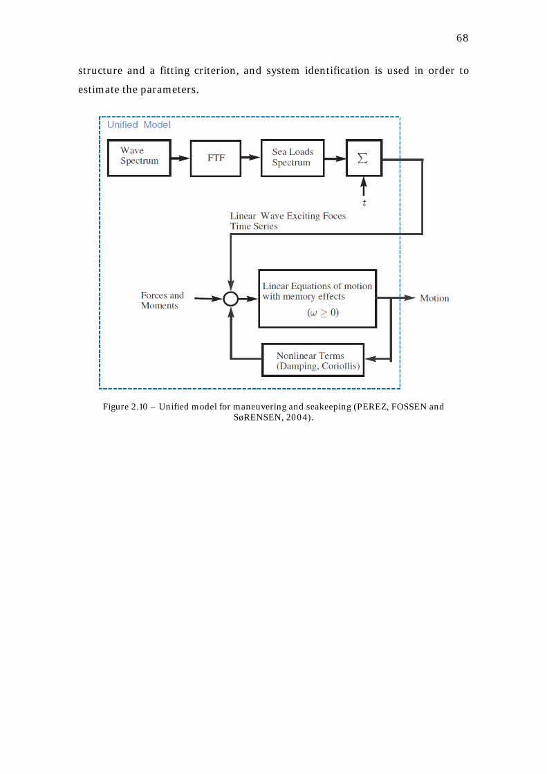
68

structure and a fitting criterion, and system identification is used in order to

estimate the parameters.

Figure 2.10 – Unified model for maneuvering and seakeeping (PEREZ, FOSSEN and

SøRENSEN, 2004).

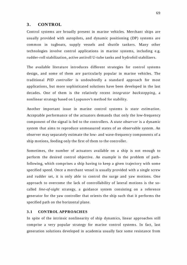
69

3. CONTROL Control systems are broadly present in marine vehicles. Merchant ships are

usually provided with autopilots, and dynamic positioning (DP) systems are

common in tugboats, supply vessels and shuttle tankers. Many other

technologies involve control applications in marine systems, including e.g.

rudder-roll stabilization, active antiroll U-tube tanks and hydrofoil stabilizers.

The available literature introduces different strategies for control systems

design, and some of them are particularly popular in marine vehicles. The

traditional PID controller is undoubtedly a standard approach for most

applications, but more sophisticated solutions have been developed in the last

decades. One of them is the relatively recent integrator backstepping, a

nonlinear strategy based on Lyapunov’s method for stability.

Another important issue in marine control systems is state estimation.

Acceptable performance of the actuators demands that only the low-frequency

component of the signal is fed to the controllers. A state observer is a dynamic

system that aims to reproduce unmeasured states of an observable system. An

observer may separately estimate the low- and wave-frequency components of a

ship motions, feeding only the first of them to the controller.

Sometimes, the number of actuators available on a ship is not enough to

perform the desired control objective. An example is the problem of path-

following, which comprises a ship having to keep a given trajectory with some

specified speed. Once a merchant vessel is usually provided with a single screw

and rudder set, it is only able to control the surge and yaw motions. One

approach to overcome the lack of controllability of lateral motions is the so-

called line-of-sight strategy, a guidance system consisting on a reference

generator for the yaw controller that orients the ship such that it performs the

specified path on the horizontal plane.

3.1 CONTROL APPROACHES

In spite of the intrinsic nonlinearity of ship dynamics, linear approaches still

comprise a very popular strategy for marine control systems. In fact, last

generation solutions developed in academia usually face some resistance from

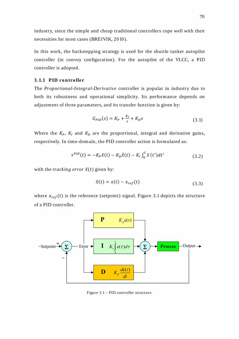
70

industry, since the simple and cheap traditional controllers cope well with their

necessities for most cases (BREIVIK, 2010).

In this work, the backstepping strategy is used for the shuttle tanker autopilot

controller (in convoy configuration). For the autopilot of the VLCC, a PID

controller is adopted.

3.1.1 PID controller

The Proportional-Integral-Derivative controller is popular in industry due to

both its robustness and operational simplicity. Its performance depends on

adjustment of three parameters, and its transfer function is given by:

𝐺𝑃𝐼𝐷(𝑠) = 𝐾𝑃 + 𝐾𝐼𝑠

+ 𝐾𝐷𝑠 (3.1)

Where the 𝐾𝑃, 𝐾𝐼 and 𝐾𝐷 are the proportional, integral and derivative gains,

respectively. In time-domain, the PID controller action is formulated as:

𝜏𝑃𝐼𝐷(𝑡) = −𝐾𝑃𝑥�(𝑡) − 𝐾𝐷𝑥�̇(𝑡) − 𝐾𝐼 ∫ 𝑥�𝑡0 (𝑡′)𝑑𝑡′ (3.2)

with the tracking error 𝑥�(𝑡) given by:

𝑥�(𝑡) = 𝑥(𝑡) − 𝑥𝑟𝑒𝑓(𝑡) (3.3)

where 𝑥𝑟𝑒𝑓(𝑡) is the reference (setpoint) signal. Figure 3.1 depicts the structure

of a PID controller.

Figure 3.1 – PID controller structure.

71

When a PID controller is used in autopilot design, care must be taken with the

so-called integrator windup phenomenon. When the actuator – in this case, the

rudder – saturates, the error continues to be integrated so that the integrator in

(3.2) “winds up”, that is, assumes a very large value (ÅSTRÖM and

HÄGGLUND, 1995). This process is illustrated in Figure 3.2. The high change in

the setpoint leads the actuator to saturation, as it may be noticed in the second

graphic. However, even after the system output reaches the reference the

actuator still keeps saturated due to the accumulated integral parcel,

represented in the curve on the bottom of the figure.

Figure 3.2 – Integrator windup phenomenon, where 𝑦 is the process output, 𝑦𝑠𝑑 is the setpoint, 𝑢 is the control signal and 𝐼 is the integral part. Extracted from (ÅSTRÖM and HÄGGLUND,

1995).

Since the windup phenomenon may lead the system to destabilization, it is

worth to avoid it by implementing some algorithms together with the controller.

An effective and relatively simple method is to establish a bound to the integral

parcel, by stopping the integration process when it reaches a predefined value.

3.1.2 Backstepping controller

Backstepping is a nonlinear strategy for control systems design through a

recursive procedure based on the Lyapunov direct method for stability. An

expedient feature is the possibility of taking advantage of some nonlinearities of

the system, instead of just cancelling them as in feedback linearization

72

approach, for instance. Therefore, dependence of the control laws on unknown

parameters of the system is diminished, together with the total amount of

energy required for the controlling action. Derivation of backstepping

formulation demands some insight on Lyapunov’s theory for determining the

stability of a system, as presented on Appendix A.

The integral backstepping method

Backstepping is a recursive technique for nonlinear control systems design, as

presented in (KRSTIC, KANELLAKOPOULOS and KOKOTOVIC, 1995). When

the system input is connected to a series of integrators, the method is called

integral backstepping. Let a nonlinear system be defined, for example, by the

following equations (FOSSEN and STRAND, 1998):

�̇�1 = 𝑓(𝑥1) + 𝑥2 (3.4) �̇�2 = 𝑢 (3.5) 𝑦 = 𝑥1 (3.6)

where 𝑥1, 𝑥2, 𝑦,𝑢 ∈ ℝ and the nonlinear function 𝑓(𝑥1) has the following form:

𝑓(𝑥1) = −𝑎0𝑥1 − 𝑎1𝑥12 − 𝑎2|𝑥1|𝑥1 (3.7)

Considering the objective of the control as to lead 𝑦(𝑡) ⟶ 0 for 𝑡 ⟶ ∞, it comes

that the desired result is to render (𝑥1, 𝑥2) = (0,−𝑓(0)) as an GAS equilibrium

point. The recursive design is divided into two steps, as the system (3.4)-(3.5)

involves two states. First, the following change of variables is introduced:

𝐳 = 𝛟(𝐱) (3.8)

where 𝐳 = [𝑧1, 𝑧2]T, 𝐱 = [𝑥1, 𝑥2]T and 𝛟 is a diffeomorphic function. For the first

step, the above transformation is defined for 𝑧1:

𝑧1 = 𝑥1 (3.9)

Then, regarding the state 𝑥2 as a virtual control input:

𝑥2 ≜ 𝛼1 + 𝑧2 (3.10)

where 𝛼1 is called stabilizing function, it comes from (3.4), (3.9) and (3.10) that:

73

�̇�1 = 𝑓(𝑥1) + 𝛼1 + 𝑧2 (3.11)

The choice of an expression for 𝛼1 is a matter of analyzing 𝑓(𝑥1) so that the

“good” nonlinearities, i.e., those that help keeping the system stable should be

kept. Meanwhile the “bad” ones (those that destabilize the system) are to be

dominated. Thus, a suitable choice for 𝛼1 could be:

𝛼1 = −[𝑘1 + 𝜅1𝑧12]𝑧1 (3.12)

with 𝑘1, 𝜅1 > 0, so that the “bad” nonlinearity 𝑎1𝑥12 of 𝑓(𝑥1) is dominated (since

the introduced term is proportional to 𝑥3), while the “good” terms 𝑎0𝑥1 and

𝑎2|𝑥1|𝑥1 are not controlled, for they are useful to attain stability to the system.

Substituting in (3.11):

�̇�1 = −(𝑎0 + 𝑎2|𝑧1| + 𝑘1)𝑧1 − 𝑎1𝑧12 − 𝜅1𝑧13 + 𝑧2 (3.13)

Considering the Lyapunov candidate function:

𝑉1 =12𝑧12 (3.14)

Time differentiation of 𝑉1 yields:

�̇�1 =𝜕𝑉1𝜕𝑧1

�̇�1 = −(𝑎0 + 𝑎2|𝑧1| + 𝑘1)𝑧12 − 𝑎1𝑧13 − 𝜅1𝑧14 + 𝑧1𝑧2 (3.15)

The second step departs from time derivation of 𝑧2. From (3.10) it comes that:

�̇�2 = �̇�2 − �̇�1 = 𝑢 − �̇�1 (3.16)

Let a Lyapunov candidate 𝑉2 be defined as:

𝑉2 = 𝑉1 +12𝑧22 (3.17)

Proceeding with the same approach as for 𝑉1:

�̇�2 = −(𝑎0 + 𝑎2|𝑧1| + 𝑘1)𝑧12 − 𝑎1𝑧13 − 𝜅1𝑧14 + 𝑧2(𝑧1 + 𝑢 − �̇�1) (3.18)

Choosing the control law 𝑢 as:

74

𝑢 = �̇�1 − 𝑘2𝑧2 − 𝑧1 (3.19)

Substitution in (3.18) yields:

�̇�2 = −(𝑎0 + 𝑎2|𝑧1| + 𝑘1)𝑧12 − 𝑎1𝑧13 − 𝜅1𝑧14 − 𝑘2𝑧22 (3.20)

which can be rewritten as:

�̇�2 = −�

𝑎12√𝜅1

𝑧1 + �𝜅1𝑧12�2−𝑎12

4𝜅1𝑧12 − (𝑎0 + 𝑎2|𝑧1| + 𝑘1)𝑧12 − 𝑘2𝑧22

≤ −�𝑎0 + 𝑘1 −𝑎12

4𝜅1� 𝑧12 − 𝑘2𝑧22

(3.21)

Finally, rendering �̇�2 < 0 is a matter of choosing the controller gains according

to the following relations:

𝜅1 > 0

𝑘1 >𝑎12

4𝜅1− 𝑎0

𝑘2 > 0

(3.22)

Such that the control design is complete. This approach will be particularized

for application in a ship autopilot on Chapter 5.

3.2 NONLINEAR PASSIVE OBSERVER

State estimation is performed by an approximate mathematical model of a real

system, corrected by the difference between measurement and estimates

multiplied by appropriate gains. Such gains must be calculated in a way to make

the observer state to converge to the real system state.

A nonlinear observer comprises a model with nonlinear equations. This is

attractive for inherently nonlinear systems, like marine vehicles, since it is not

necessary to linearize the equations around a discretized envelope of heading

angles, in opposition to the procedure involving a linear observer (e.g. Kalman

Filter) (FOSSEN, 2002).

The adopted formulation was based in (FOSSEN and STRAND, 1999) and

(ZAKARTCHOUK JR, 2010), and applies passivity theory in order to assure that

the estimates converge to the real system state. That is, the observer gains are

75

determined as to assign passivity to the error dynamics, ensuring that they

asymptotically converge to zero.

Such references, however, are developed for dynamic positioning (DP)

applications, such that their formulation disregards the Coriolis and centripetal

matrix under assumption of low velocities. Here, the system to be observed is an

underway ship, such that the surge velocity cannot be disregarded. Proper

linearization of that matrix around the surge service velocity ensures that the

necessary assumptions for the observer functionality are fulfilled, though.

3.2.1 Observer model

The maneuvering model in 3 DOF (section 2.7.1) may be simplified according

to:

𝐌�̇� + 𝐍𝛎 = 𝛕𝑒𝑛𝑣 + 𝛕𝑐𝑜𝑛

�̇� = 𝐉(𝛈)𝛎 (3.23)

where the influence of the current speed in radiation forces was neglected and

the damping matrix was admitted as being purely linear. The inertia matrix 𝐌

is considered to be strictly positive and symmetric14

, that is, 𝐌 = 𝐌T > 0 and is

composed by both rigid-body and added-mass components, i.e., 𝐌 =

(𝐌𝑅𝐵 + 𝐀0), while 𝐍 is the sum of the linear damping terms and the Coriolis and

centripetal matrix linearized around 𝛎ℎ = [𝑈𝑠 0 0]T, 𝑈𝑠 being the service

speed:

𝐍 = 𝐂 + 𝐃 (3.24)

𝐂 = �0 0 00 0 (𝑚− 𝑋�̇�)𝑈𝑠0 −(𝑚− 𝑋�̇�)𝑈𝑠 0

� (3.25)

𝐃 = −�𝑋𝑢 0 00 𝑌𝑛 𝑌𝑟0 𝑁𝑣 𝑁𝑟

� (3.26)

with the damping coefficients as defined in section 2.5.2. It is important to

observe that 𝐂 = −𝐂T, such that:

14 The added mass matrix is actually non-symmetric for advancing ships, but since surge speedy is moderate it will be admitted as symmetric in this formulation.

76

(𝐍 + 𝐍T) = (𝐃 + 𝐂 + 𝐃T + 𝐂T) = (𝐃 + 𝐃T) (3.27)

This result is mandatory for the extension of the formulation in (FOSSEN and

STRAND, 1999) to the case of an underway ship.

The vector of environmental loads 𝛕𝑒𝑛𝑣 is the body-fixed projection of a bias

forces and moments vector 𝐛 ∈ ℝ3, admitted as a slowly varying Gaussian

process, that is:

𝛕𝑒𝑛𝑣 = 𝐉T(𝛈)𝐛 (3.28) �̇� = −𝐓−1𝐛 + 𝚿𝐧 (3.29)

with 𝐓 ∈ ℝ3𝑋3 being a diagonal matrix with time constants, 𝚿 ∈ ℝ3𝑋3 a matrix of

gains and 𝐧 ∈ ℝ3 a vector of zero-mean white Gaussian noise.

Finally, the model for WF-motions arises from an approximation for the ship

response power spectrum 𝑃𝑖:

𝑃𝑖 = �ℎ𝑤𝑓𝑖 (𝑗𝜔)�2 (3.30)

𝑖 = 1,2,3, with the transfer function ℎ𝑤𝑓𝑖 (𝑠) given by (FOSSEN, 2002):

ℎ𝑤𝑓𝑖 (𝑠) = 𝜎𝑖𝑠𝑠2+2𝜁𝑖𝜔0𝑖𝑠+𝜔𝑜𝑖

2 (3.31)

𝜔0𝑖 and 𝜁𝑖 being the modal frequency and damping for the approximated

spectrum, respectively, and 𝜎𝑖 a parameter for adjustment of the approximation.

Representing (3.31) in a state-space model one gets:

�̇� = 𝛀𝛏 + 𝚺𝐰

𝜼𝑤𝑓 = 𝚪𝝃 (3.32)

where 𝝃 ∈ ℝ6 is the state vector, 𝜼𝑤𝑓 ∈ ℝ3 is the output vector with the WF-

motions, 𝐰 ∈ ℝ3 is a vector of zero-mean white gaussian noise and the matrices

𝛀, 𝚺 and 𝚪 are defined as following:

𝛀 = �𝟎3X3 𝐈3𝑋3𝛀21 𝛀22

� (3.33)

77

𝚺 = �𝟎3X3𝚺2� (3.34)

𝚪 = [𝟎3X3 𝐈3𝑋3] (3.35)

with the matrices 𝛀21,𝛀22,𝚺2 ∈ ℝ3𝑋3 given by:

𝛀21 = −�𝜔01 0 0

0 𝜔02 00 0 𝜔03

� (3.36)

𝛀22 = − �2𝜁1𝜔01 0 0

0 2𝜁2𝜔02 00 0 2𝜁3𝜔03

� (3.37)

𝚺2 = �𝜎1 0 00 𝜎2 00 0 𝜎3

� (3.38)

3.2.2 Observer design

In this work, the observer is intended to separately estimate the low- and wave-

frequency components of a ship motions. Also, the vector of bias loads is also

estimated by the observer, so that it may be considered as feedforward in the

controller.

With basis on the model presented in the last section, the observer equations

may be defined as following:

𝝃�̇ = 𝛀𝛏� + 𝐊1𝐲� (3.39)

𝛈�̇ = 𝐉(𝐲)𝛎� + 𝐊2𝐲� (3.40)

�̇̂� = −𝐓−1�̂� + 𝚲𝐲� (3.41)

𝐌𝛎�̇ = −𝐍𝛎 + 𝐉T(𝐲)𝐛 + 𝐉T(𝐲)𝛋𝐲� + 𝛕𝑐𝑜𝑛 (3.42)

𝐲�̇ = 𝛈� + 𝚪𝛏� (3.43)

where 𝐲 ∈ ℝ3 is the measurement, 𝐲� = 𝐲 − 𝐲� ∈ ℝ3 is the position estimation

error and 𝐊1 ∈ ℝ6𝑋3, 𝐊2 ∈ ℝ3𝑋3, 𝚲 ∈ ℝ3𝑋3 and 𝛋 ∈ ℝ3𝑋3 are gain matrices for the

observer, whose calculation are based on the passivity of the estimation error

dynamics.

3.2.3 Gains determination

78

Let the gain matrices have the following structure:

𝐊1 =

⎣⎢⎢⎢⎢⎢⎡𝑘11𝑜 0 00 𝑘12𝑜 00 0 𝑘13𝑜

𝑘21𝑜 0 00 𝑘22𝑜 00 0 𝑘23𝑜 ⎦

⎥⎥⎥⎥⎥⎤

(3.44)

𝐊2 = �𝑘31𝑜 0 00 𝑘32𝑜 00 0 𝑘33𝑜

� (3.45)

𝚲 = �𝜆1𝑜 0 00 𝜆2𝑜 00 0 𝜆3𝑜

� (3.46)

𝛋 = �𝜅1𝑜 0 00 𝜅2𝑜 00 0 𝜅3𝑜

� (3.47)

The following procedure ensures that the estimates converge to the real states

according to passivity theory, through proper determination for the gains above.

Also, the gains are chosen in a way that the observer works as a notch filter,

improving its performance on wave filtering. Let 𝜔0𝑖 be the dominating

frequencies of the responses and 𝜔𝑐𝑖 > 𝜔0𝑖 the desired filter cut-off frequency.

Also, let 𝜁𝑛𝑖 > 𝜁𝑖 be the notch effect parameter. The gains of 𝐊1 and 𝐊2 are then

defined according to:

𝑘1𝑖𝑜 = −2𝜔𝑐𝑖(𝜁𝑛𝑖 − 𝜁𝑖)1𝜔0𝑖

(3.48)

𝑘2𝑖𝑜 = 2𝜔0𝑖(𝜁𝑛𝑖 − 𝜁𝑖) (3.49)

𝑘3𝑖𝑜 = 𝜔𝑐𝑖 (3.50)

Once fulfilled the above requirements, the remainder gains should be assigned

as to satisfy the following relation:

1𝑇𝑖≪𝜆𝑖𝜅𝑖

< 𝜔0 < 𝜔𝑐𝑖 (3.51)

79

where 𝑇𝑖 ≫ 1 are the terms of the 𝐓 matrix on equation (3.29). The above

choices for the observer gains are enough to satisfy the requirements for

passivity, as developed in (FOSSEN and STRAND, 1999), where the proofs and

stability analyses may be found.

3.3 THE LINE-OF-SIGHT GUIDANCE SYSTEM

A popular application of control theory in marine vehicles is the design of

autopilots, systems intended to control the ship heading 𝜓 by means of its

rudder(s). Therefore, for a given reference 𝜓𝑟𝑒𝑓, the objective of an autopilot is

to render the heading offset 𝜖𝜓 to zero, that is:

𝜖𝜓 = 𝜓𝑟𝑒𝑓 − 𝜓 ⟶ 0 𝑓𝑜𝑟 𝑡 ⟶ ∞ (3.52)

Besides, an autopilot generally also controls the surge velocity of the ship, by

increasing or decreasing the propeller(s) rotation in order to keep the required

speed 𝑢𝑟𝑒𝑓. Therefore, a ship provided with an autopilot may keep constant

speed and headings without interference of a human operator.

Maintaining a constant heading, however, is not enough to keep a ship over a

given trajectory. In fact, the vessel may drift away from it due bias loads from

current, wind and second order wave effects, even though it preserves the

commanded value for 𝜓𝑟𝑒𝑓. The reason for this is that keeping a vessel

advancing over a desired path (including its orientation) is a problem in 3 DOF,

which cannot be simultaneously controlled by means of independent control

inputs in only 2 DOF. That is, a ship provided with only main propellers and

rudders is underactuated for the problem of horizontal motions (BREIVIK,

2003).

A relatively simple way to overcome this problem is by usage of the line-of-sight

(LOS) guidance system, which consists in a methodology to generate a reference

heading 𝜓𝑟𝑒𝑓 such that the ship points to the trajectory. That is, when the ship

drifts away from the desired path, the value for 𝜓𝑟𝑒𝑓 is calculated as to orient

her back to it.

The first step for applying the LOS strategy is to divide the desired trajectory in

waypoints. Then, the ship current position is compared with the so-called LOS

position 𝑝𝑙𝑜𝑠 = (𝑥𝑙𝑜𝑠, 𝑦𝑙𝑜𝑠), which corresponds to a point located on the segment

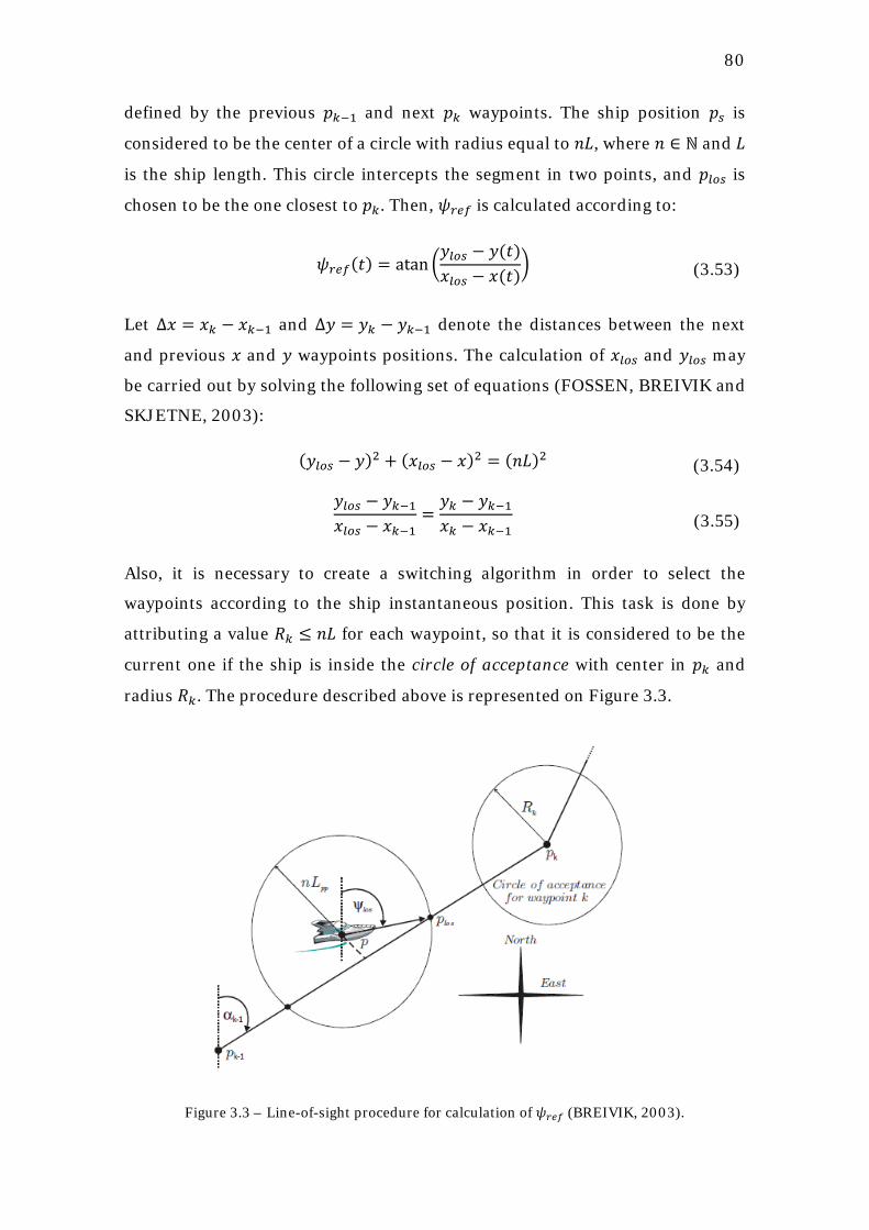
80

defined by the previous 𝑝𝑘−1 and next 𝑝𝑘 waypoints. The ship position 𝑝𝑠 is

considered to be the center of a circle with radius equal to 𝑛𝐿, where 𝑛 ∈ ℕ and 𝐿

is the ship length. This circle intercepts the segment in two points, and 𝑝𝑙𝑜𝑠 is

chosen to be the one closest to 𝑝𝑘. Then, 𝜓𝑟𝑒𝑓 is calculated according to:

𝜓𝑟𝑒𝑓(𝑡) = atan �𝑦𝑙𝑜𝑠 − 𝑦(𝑡)𝑥𝑙𝑜𝑠 − 𝑥(𝑡)

� (3.53)

Let Δ𝑥 = 𝑥𝑘 − 𝑥𝑘−1 and Δ𝑦 = 𝑦𝑘 − 𝑦𝑘−1 denote the distances between the next

and previous 𝑥 and 𝑦 waypoints positions. The calculation of 𝑥𝑙𝑜𝑠 and 𝑦𝑙𝑜𝑠 may

be carried out by solving the following set of equations (FOSSEN, BREIVIK and

SKJETNE, 2003):

(𝑦𝑙𝑜𝑠 − 𝑦)2 + (𝑥𝑙𝑜𝑠 − 𝑥)2 = (𝑛𝐿)2 (3.54)

𝑦𝑙𝑜𝑠 − 𝑦𝑘−1𝑥𝑙𝑜𝑠 − 𝑥𝑘−1

=𝑦𝑘 − 𝑦𝑘−1𝑥𝑘 − 𝑥𝑘−1

(3.55)

Also, it is necessary to create a switching algorithm in order to select the

waypoints according to the ship instantaneous position. This task is done by

attributing a value 𝑅𝑘 ≤ 𝑛𝐿 for each waypoint, so that it is considered to be the

current one if the ship is inside the circle of acceptance with center in 𝑝𝑘 and

radius 𝑅𝑘. The procedure described above is represented on Figure 3.3.

Figure 3.3 – Line-of-sight procedure for calculation of 𝜓𝑟𝑒𝑓 (BREIVIK, 2003).

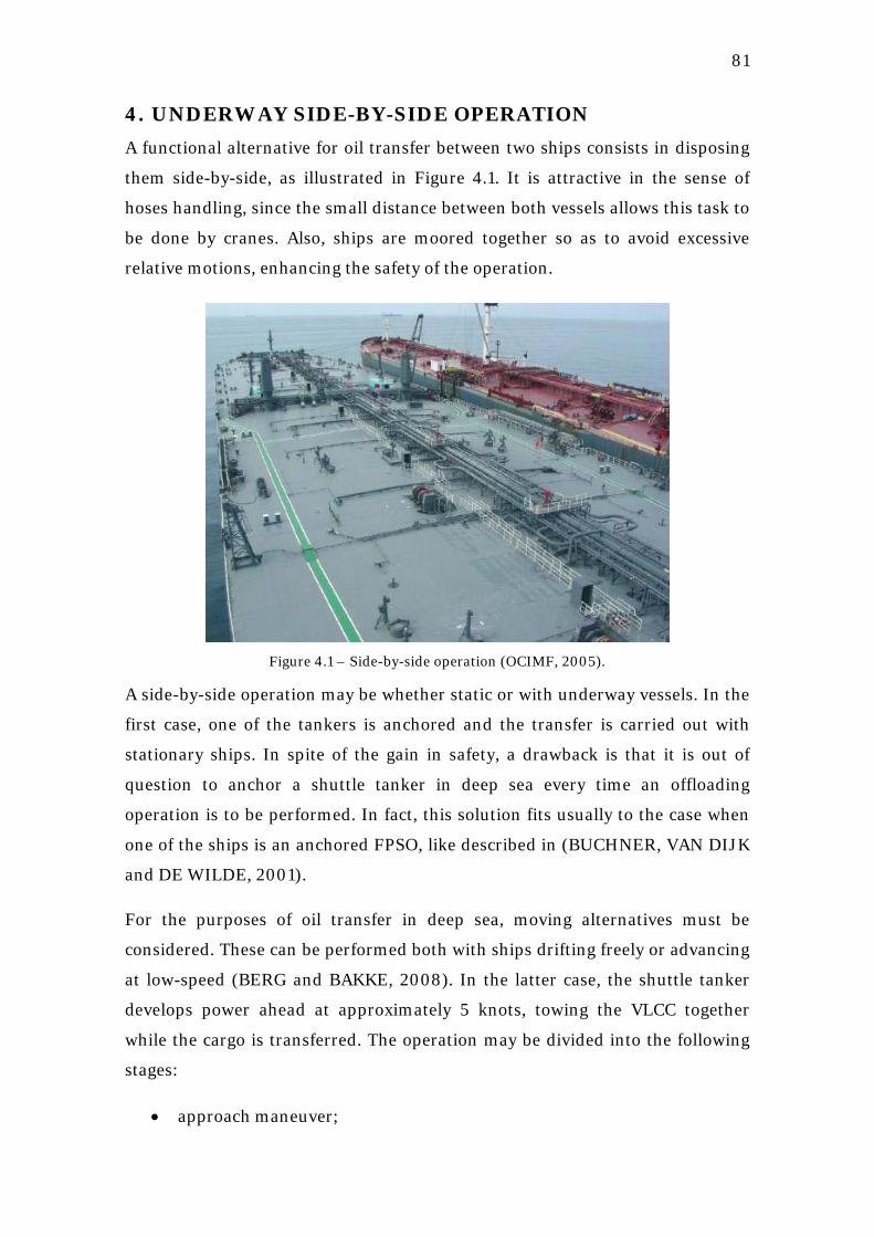
81

4. UNDERWAY SIDE-BY-SIDE OPERATION A functional alternative for oil transfer between two ships consists in disposing

them side-by-side, as illustrated in Figure 4.1. It is attractive in the sense of

hoses handling, since the small distance between both vessels allows this task to

be done by cranes. Also, ships are moored together so as to avoid excessive

relative motions, enhancing the safety of the operation.

Figure 4.1 – Side-by-side operation (OCIMF, 2005).

A side-by-side operation may be whether static or with underway vessels. In the

first case, one of the tankers is anchored and the transfer is carried out with

stationary ships. In spite of the gain in safety, a drawback is that it is out of

question to anchor a shuttle tanker in deep sea every time an offloading

operation is to be performed. In fact, this solution fits usually to the case when

one of the ships is an anchored FPSO, like described in (BUCHNER, VAN DIJK

and DE WILDE, 2001).

For the purposes of oil transfer in deep sea, moving alternatives must be

considered. These can be performed both with ships drifting freely or advancing

at low-speed (BERG and BAKKE, 2008). In the latter case, the shuttle tanker

develops power ahead at approximately 5 knots, towing the VLCC together

while the cargo is transferred. The operation may be divided into the following

stages:

• approach maneuver;

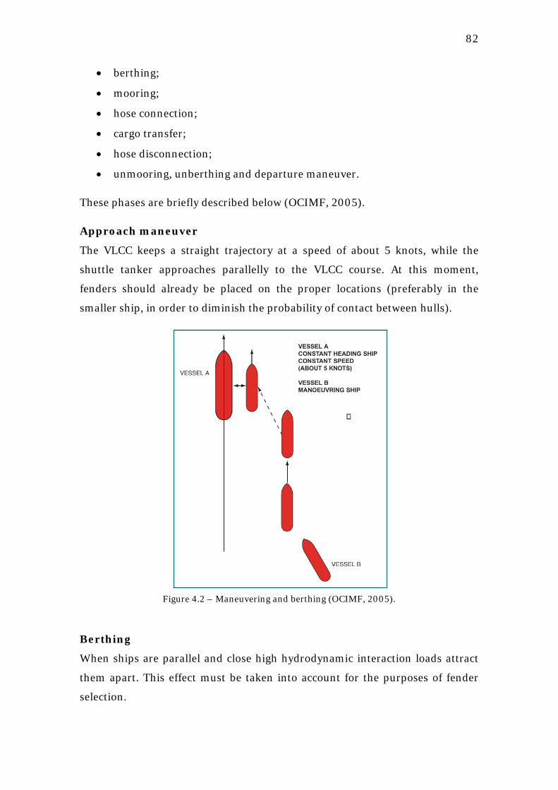
82

• berthing;

• mooring;

• hose connection;

• cargo transfer;

• hose disconnection;

• unmooring, unberthing and departure maneuver.

These phases are briefly described below (OCIMF, 2005).

Approach maneuver

The VLCC keeps a straight trajectory at a speed of about 5 knots, while the

shuttle tanker approaches parallelly to the VLCC course. At this moment,

fenders should already be placed on the proper locations (preferably in the

smaller ship, in order to diminish the probability of contact between hulls).

Figure 4.2 – Maneuvering and berthing (OCIMF, 2005).

Berthing

When ships are parallel and close high hydrodynamic interaction loads attract

them apart. This effect must be taken into account for the purposes of fender

selection.

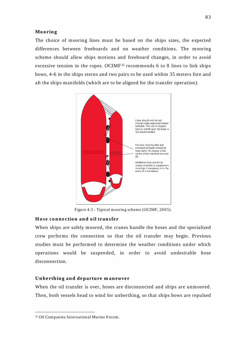
83

Mooring

The choice of mooring lines must be based on the ships sizes, the expected

differences between freeboards and on weather conditions. The mooring

scheme should allow ships motions and freeboard changes, in order to avoid

excessive tension in the ropes. OCIMF15

recommends 6 to 8 lines to link ships

bows, 4-6 in the ships sterns and two pairs to be used within 35 meters fore and

aft the ships manifolds (which are to be aligned for the transfer operation).

Figure 4.3 - Typical mooring scheme (OCIMF, 2005).

Hose connection and oil transfer

When ships are safely moored, the cranes handle the hoses and the specialized

crew performs the connection so that the oil transfer may begin. Previous

studies must be performed to determine the weather conditions under which

operations would be suspended, in order to avoid undesirable hose

disconnection.

Unberthing and departure maneuver

When the oil transfer is over, hoses are disconnected and ships are unmoored.

Then, both vessels head to wind for unberthing, so that ships bows are repulsed

15 Oil Companies International Marine Forum.

84

away from each other. Separation is then performed and each ship may

maneuver to follow its destination.

The present chapter focuses on the dynamics involved during the transfer

phase. Thus, the next sections will treat the equations of motions, models for

mooring lines and fenders and a discussion on hydrodynamic interactions.

Subsequently, simulation results for different conditions are presented and

discussed.

4.1 HYDRODYNAMIC INTERACTIONS

The condition of two advancing ships at a separation distance as short as 3

meters is not without complications, from the hydrodynamics point-of-view. In

fact, important interaction effects are involved due to the fluid behavior between

the vessels. They can be divided into two main classes of phenomena, viz.:

• suction loads, arisen from the alteration off the pressure field due to the

fluid behavior between the hulls, in calm water;

• wave interaction, that is, effects related to the wave-field generated

between hulls.

The influence of the effects listed above is determinant for the dynamics of a

side-by-side operation. Thus, a discussion on this topic is presented in the

following subsections.

4.1.1 Suction loads

When two ships navigate side-by-side and with zero relative speed, the flow

between them is disturbed such that the resulting pressure field inducts a

suction force in the hulls. A simplified explanation for this phenomenon comes

from the faster velocity of the fluid between hulls. This would lead to a reduction

on the pressure field and, consequently, to the suction forces.

However, studies concerning this kind of loads for the specific situation

approached in the presented work – viz., deep-waters and zero relative speed –

are incipient. The main studies on the area relate to encounter/overpassing

maneuvers in shallow waters and with a separation distance comparable to the

ships beams. Other publications tackle the underway replenishment operations,

which consist in two ships navigating parallel and in deep waters, but at a

distance of the order of half a ship length.

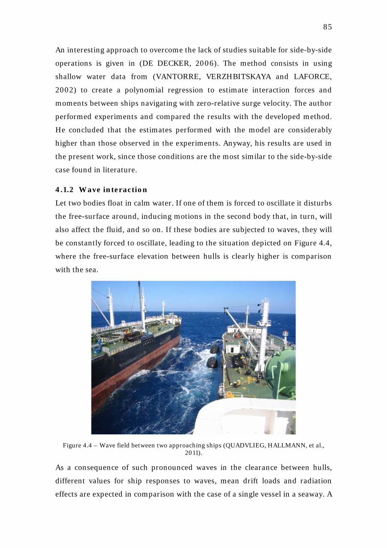
85

An interesting approach to overcome the lack of studies suitable for side-by-side

operations is given in (DE DECKER, 2006). The method consists in using

shallow water data from (VANTORRE, VERZHBITSKAYA and LAFORCE,

2002) to create a polynomial regression to estimate interaction forces and

moments between ships navigating with zero-relative surge velocity. The author

performed experiments and compared the results with the developed method.

He concluded that the estimates performed with the model are considerably

higher than those observed in the experiments. Anyway, his results are used in

the present work, since those conditions are the most similar to the side-by-side

case found in literature.

4.1.2 Wave interaction

Let two bodies float in calm water. If one of them is forced to oscillate it disturbs

the free-surface around, inducing motions in the second body that, in turn, will

also affect the fluid, and so on. If these bodies are subjected to waves, they will

be constantly forced to oscillate, leading to the situation depicted on Figure 4.4,

where the free-surface elevation between hulls is clearly higher is comparison

with the sea.

Figure 4.4 – Wave field between two approaching ships (QUADVLIEG, HALLMANN, et al.,

2011).

As a consequence of such pronounced waves in the clearance between hulls,

different values for ship responses to waves, mean drift loads and radiation

effects are expected in comparison with the case of a single vessel in a seaway. A

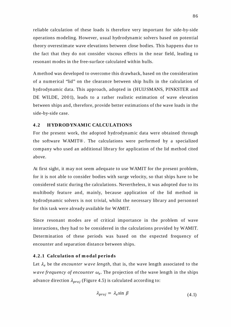
86

reliable calculation of these loads is therefore very important for side-by-side

operations modeling. However, usual hydrodynamic solvers based on potential

theory overestimate wave elevations between close bodies. This happens due to

the fact that they do not consider viscous effects in the near field, leading to

resonant modes in the free-surface calculated within hulls.

A method was developed to overcome this drawback, based on the consideration

of a numerical “lid” on the clearance between ship hulls in the calculation of

hydrodynamic data. This approach, adopted in (HUIJSMANS, PINKSTER and

DE WILDE, 2001), leads to a rather realistic estimation of wave elevation

between ships and, therefore, provide better estimations of the wave loads in the

side-by-side case.

4.2 HYDRODYNAMIC CALCULATIONS

For the present work, the adopted hydrodynamic data were obtained through

the software WAMIT®. The calculations were performed by a specialized

company who used an additional library for application of the lid method cited

above.

At first sight, it may not seem adequate to use WAMIT for the present problem,

for it is not able to consider bodies with surge velocity, so that ships have to be

considered static during the calculations. Nevertheless, it was adopted due to its

multibody feature and, mainly, because application of the lid method in

hydrodynamic solvers is not trivial, whilst the necessary library and personnel

for this task were already available for WAMIT.

Since resonant modes are of critical importance in the problem of wave

interactions, they had to be considered in the calculations provided by WAMIT.

Determination of these periods was based on the expected frequency of

encounter and separation distance between ships.

4.2.1 Calculation of modal periods

Let 𝜆𝑒 be the encounter wave length, that is, the wave length associated to the

wave frequency of encounter 𝜔𝑒. The projection of the wave length in the ships

advance direction 𝜆𝑝𝑟𝑜𝑗 (Figure 4.5) is calculated according to:

𝜆𝑝𝑟𝑜𝑗 = 𝜆𝑒sin 𝛽 (4.1)

87

Figure 4.5 – Ships advancing in waves16

The present case may be considered analogous to that of resonant modes in the

free-surface of a tank with vertical walls. In this situation, the resonant wave

lengths are given by:

.

𝜆𝑝𝑟𝑜𝑗 =2𝑑𝑛

(4.2)

where 𝑛 ∈ ℕ∗ is the natural mode and 𝑑 is the distance between hulls, as

depicted on Figure 4.5. From the dispersion relation one has:

𝜆𝑒 =2𝜋𝑔𝜔𝑒2

(4.3)

Combining (4.1), (4.2) and (4.3) the following expression for the frequency of

encounter 𝜔𝑒 is obtained:

𝜔𝑒 = �𝜋𝑔𝑛 sin𝛽𝑑

(4.4)

However, 𝜔𝑒 may also be written in terms of 𝛽, 𝑈 and 𝜔0 (the frequency for

zero-velocity) through its definition:

16 It is important to point out that the coordinate system adopted in WAMIT is different from the Earth-fixed frame utilized in this work, as defined in section 2.2. The necessary transformations are performed before the data is used in the developed model.

88

𝜔𝑒 = �𝜔0 −𝜔02

𝑔𝑈 cos𝛽� (4.5)

Equating (4.4) and (4.5):

�𝜔0 −𝜔02

𝑔𝑈 cos𝛽� = �𝜋𝑔𝑛 sin𝛽

𝑑 (4.6)

So that the modal frequencies 𝜔𝑛 may be found according to:

𝑈𝑔

cos𝛽 𝜔𝑛2 − 𝜔𝑛 + �𝜋𝑔𝑛 sin𝛽𝑑

= 0 (4.7)

for 𝜔𝑛 > 𝜔𝑛2

𝑔𝑈 cos𝛽, or:

𝑈𝑔

cos𝛽 𝜔𝑛2 − 𝜔𝑛 − �𝜋𝑔𝑛 sin𝛽𝑑

= 0 (4.8)

if 𝜔𝑛 < 𝜔𝑛2

𝑔𝑈 cos𝛽 holds. Therefore, for a given distance 𝑑 between ships and

their nominal surge velocity 𝑈 the roots of the equations above are found by

varying those values of 𝛽 used in WAMIT calculations and, typically, for the first

two modal periods (i.e., 𝑛 = 1,2). If the period 𝑇𝑛 = 2𝜋/𝜔𝑛 lies inside the

interval specified for the calculations, it should also be considered for the

correspondent separation distance and surge velocity.

4.2.2 The lid method

Attenuation of the resonant interaction effects in the gap between two ships may

be done by consideration of a numerical lid over the free-surface, as depicted on

Figure 4.6. This lid is an additional structure with a sufficient number of

generalized modes, as to feature a hinged behavior that allows reproduction of

the free-surface elevation along the gap length. By representing the free-surface

with Chebyshev polynomials, the proper number of generalized modes may be

determined as being the product of the number of Chebyshev modes in the

longitudinal and lateral directions (NYX KNOWLEDGE, 2011).

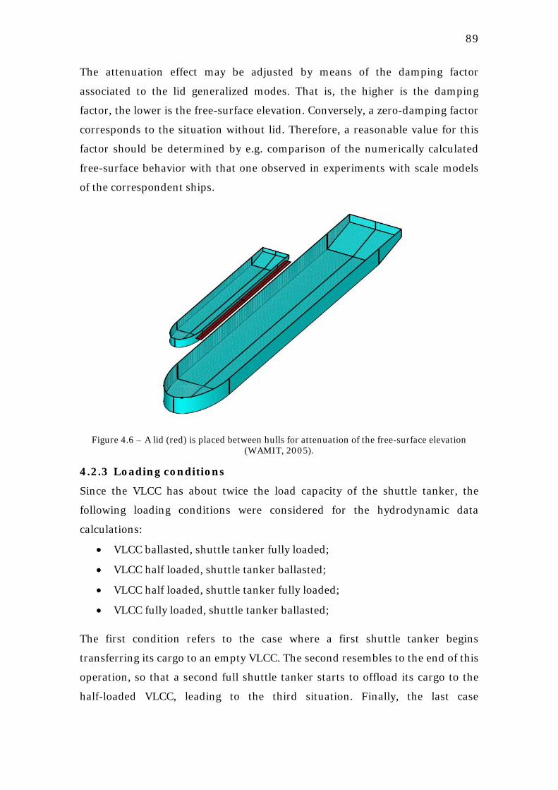
89

The attenuation effect may be adjusted by means of the damping factor

associated to the lid generalized modes. That is, the higher is the damping

factor, the lower is the free-surface elevation. Conversely, a zero-damping factor

corresponds to the situation without lid. Therefore, a reasonable value for this

factor should be determined by e.g. comparison of the numerically calculated

free-surface behavior with that one observed in experiments with scale models

of the correspondent ships.

Figure 4.6 – A lid (red) is placed between hulls for attenuation of the free-surface elevation (WAMIT, 2005).

4.2.3 Loading conditions

Since the VLCC has about twice the load capacity of the shuttle tanker, the

following loading conditions were considered for the hydrodynamic data

calculations:

• VLCC ballasted, shuttle tanker fully loaded;

• VLCC half loaded, shuttle tanker ballasted;

• VLCC half loaded, shuttle tanker fully loaded;

• VLCC fully loaded, shuttle tanker ballasted;

The first condition refers to the case where a first shuttle tanker begins

transferring its cargo to an empty VLCC. The second resembles to the end of this

operation, so that a second full shuttle tanker starts to offload its cargo to the

half-loaded VLCC, leading to the third situation. Finally, the last case

90

characterizes the situation where the VLCC is completely full, after having

received all the oil from both shuttle tankers.

4.3 DYNAMICS

A dynamic model for side-by-side simulations will now be presented based on

(SOUZA and MORISHITA, 2011). Once the wave interaction effects arise from

the waves irradiated by both bodies, they result in coupled added mass and

potential damping matrices. That is, some coefficients relate to the motions of a

ship with the radiation forces exerted on the other one. This effect is considered

by means of coupled equations of motions. Also, the formulation includes

models for the most meaningful loads involved in the operations.

4.3.1 Equations of motions

The condition of two moored ships advancing in waves is a typical situation

where the unified model for maneuvering and seakeeping presented in section

2.7.3 must be used. Therefore, equations (2.122) are adapted for the case of two

ships with coupled motions. Then, let the 12-dimension state vectors be defined

as:

𝛈𝑆𝐵𝑆 = �𝛈𝑉𝐿𝐶𝐶T ,𝛈𝑆𝑇T �

T

𝛎𝑆𝐵𝑆 = �𝛎𝑉𝐿𝐶𝐶T , 𝛎𝑆𝑇T �T

(4.9)

where each of the vectors for both the VLLC and the shuttle tanker correspond

to the definitions of (2.1) and (2.2). The equations of motion are then written

according to:

�̇�𝑉𝐿𝐶𝐶 = 𝐉𝑏𝑛�𝛈2,𝑉𝐿𝐶𝐶�𝛎𝑉𝐿𝐶𝐶

�̇�𝑆𝑇 = 𝐉𝑏𝑛�𝛈2,𝑆𝑇�𝛎𝑆𝑇 (4.10)

[𝐌𝑅𝐵 + 𝐀(∞)]�̇�𝑠𝑏𝑠 + [𝐂𝑅𝐵 + 𝐂𝐴]𝛎𝑠𝑏𝑠 + 𝛍 + 𝐆𝛈𝑠𝑏𝑠 = 𝛕 (4.11)

where 𝛈2,𝑉𝐿𝐶𝐶 and 𝛈2,𝑆𝑇 are the Euler angles vectors for the VLCC and the shuttle

tanker, respectively, and the matrices and load vector on (4.11) are defined as:

𝐌𝑅𝐵 = �

𝐌𝑅𝐵,𝑉𝐿𝐶𝐶 𝟎6𝑋6𝟎6𝑋6 𝐌𝑅𝐵,𝑆𝑇

�

𝐀(∞) = �𝐀(∞)𝑉𝐿𝐶𝐶 𝐀(∞)𝑉𝐿𝐶𝐶,𝑆𝑇𝐀(∞)𝑆𝑇,𝑉𝐿𝐶𝐶 𝐀(∞)𝑆𝑇

�

(4.12)

91

𝐂𝑅𝐵 = �𝐂𝑅𝐵,𝑆𝑇 𝟎6𝑋6𝟎6𝑋6 𝐂𝑅𝐵,𝑆𝑇

� (4.13)

𝐃 = �𝐃𝑉𝐿𝐶𝐶 𝐃𝑉𝐿𝐶𝐶,𝑆𝑇𝐃𝑆𝑇,𝑉𝐿𝐶𝐶 𝐃𝑆𝑇

� (4.14)

𝛍 = � 𝐊(𝑡 − 𝜏)𝛿𝛎(𝜏)𝑑𝜏

𝑡

0

𝐊(𝑡) = �𝐊(𝑡)𝑉𝐿𝐶𝐶 𝐊(𝑡)𝑉𝐿𝐶𝐶,𝑆𝑇𝐊(𝑡)𝑆𝑇,𝑉𝐿𝐶𝐶 𝐊(𝑡)𝑆𝑇

� (4.15)

𝐆 = �𝐆𝑉𝐿𝐶𝐶 𝟎6𝑋6𝟎6𝑋6 𝐆𝑆𝑇

� (4.16)

𝛕 = �𝛕𝑉𝐿𝐶𝐶T , 𝛕𝑆𝑇T �T

(4.17)

where the cross-terms in (4.12) and (4.14) represent the hydrodynamic coupling

explained above. Each of the generalized force vectors 𝛕𝑉𝐿𝐶𝐶 and 𝛕𝑆𝑇 are

composed by the following terms:

• Hydrodynamic suction loads

• Fenders loads

• Mooring loads

• Environmental loads

4.3.2 Hydrodynamic suction loads

The model adopted in the present work is based on the expressions developed in

(DE DECKER, 2006), which are dependent on the coefficients 𝐶ℎ,𝑋, 𝐶ℎ,𝑌 and

𝐶ℎ,𝑁, estimated by a polynomial regression of experimental data:

𝑋ℎ𝑑𝑙,𝑠 = 𝐶ℎ,𝑋12

𝜌𝑤𝑎𝑡𝑒𝑟𝐵𝑠𝑇𝑠𝑈𝑉𝐿𝐶𝐶𝑈𝑆𝑇

𝑌ℎ𝑑𝑙,𝑠 = 𝐶ℎ,𝑌12

𝜌𝑤𝑎𝑡𝑒𝑟𝐵𝑠𝑇𝑠𝑈𝑉𝐿𝐶𝐶𝑈𝑆𝑇

𝑁ℎ𝑑𝑙,𝑠 = 𝐶ℎ,𝑁12

𝜌𝑤𝑎𝑡𝑒𝑟𝐵𝑠𝐿𝑠𝑇𝑠𝑈𝑉𝐿𝐶𝐶𝑈𝑆𝑇

(4.18)

where 𝐵𝑠, 𝑇𝑠 and 𝐿𝑠 refer respectively to the beam, draft and length of ship 𝑠

(that may be both VLCC or the shuttle tanker). The velocities 𝑈 are taken into

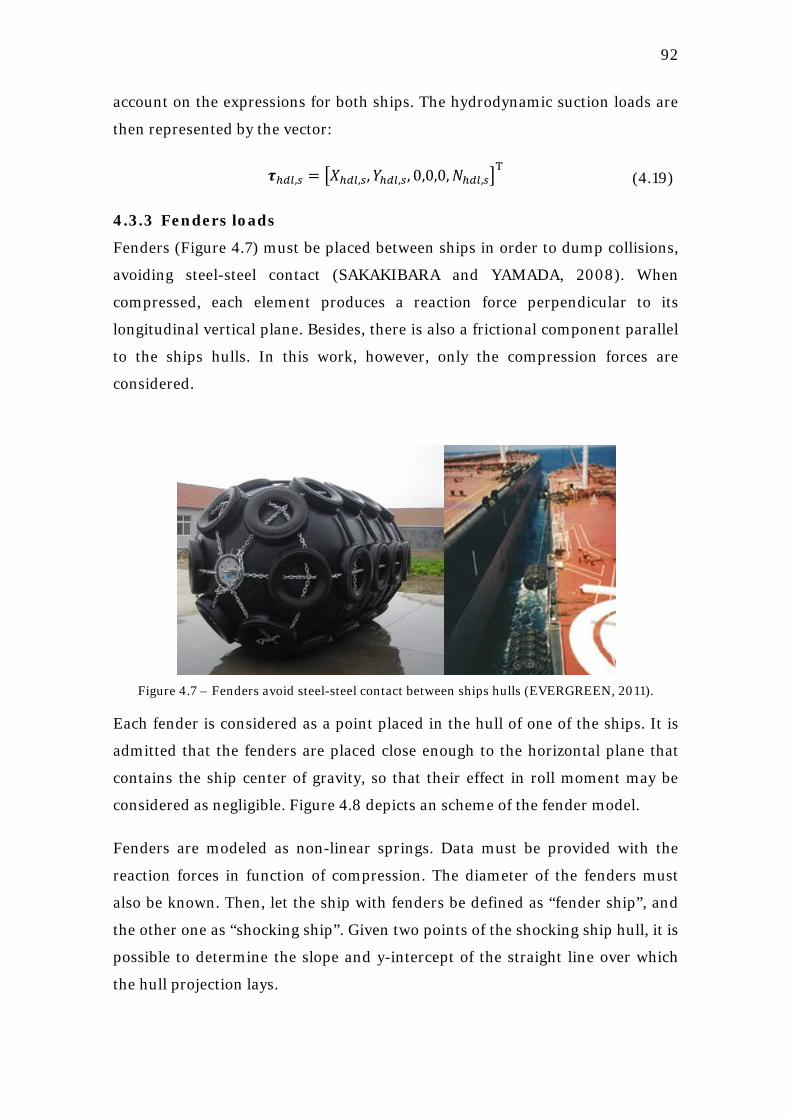
92

account on the expressions for both ships. The hydrodynamic suction loads are

then represented by the vector:

𝝉ℎ𝑑𝑙,𝑠 = �𝑋ℎ𝑑𝑙,𝑠,𝑌ℎ𝑑𝑙,𝑠, 0,0,0,𝑁ℎ𝑑𝑙,𝑠�T

(4.19)

4.3.3 Fenders loads

Fenders (Figure 4.7) must be placed between ships in order to dump collisions,

avoiding steel-steel contact (SAKAKIBARA and YAMADA, 2008). When

compressed, each element produces a reaction force perpendicular to its

longitudinal vertical plane. Besides, there is also a frictional component parallel

to the ships hulls. In this work, however, only the compression forces are

considered.

Figure 4.7 – Fenders avoid steel-steel contact between ships hulls (EVERGREEN, 2011).

Each fender is considered as a point placed in the hull of one of the ships. It is

admitted that the fenders are placed close enough to the horizontal plane that

contains the ship center of gravity, so that their effect in roll moment may be

considered as negligible. Figure 4.8 depicts an scheme of the fender model.

Fenders are modeled as non-linear springs. Data must be provided with the

reaction forces in function of compression. The diameter of the fenders must

also be known. Then, let the ship with fenders be defined as “fender ship”, and

the other one as “shocking ship”. Given two points of the shocking ship hull, it is

possible to determine the slope and y-intercept of the straight line over which

the hull projection lays.

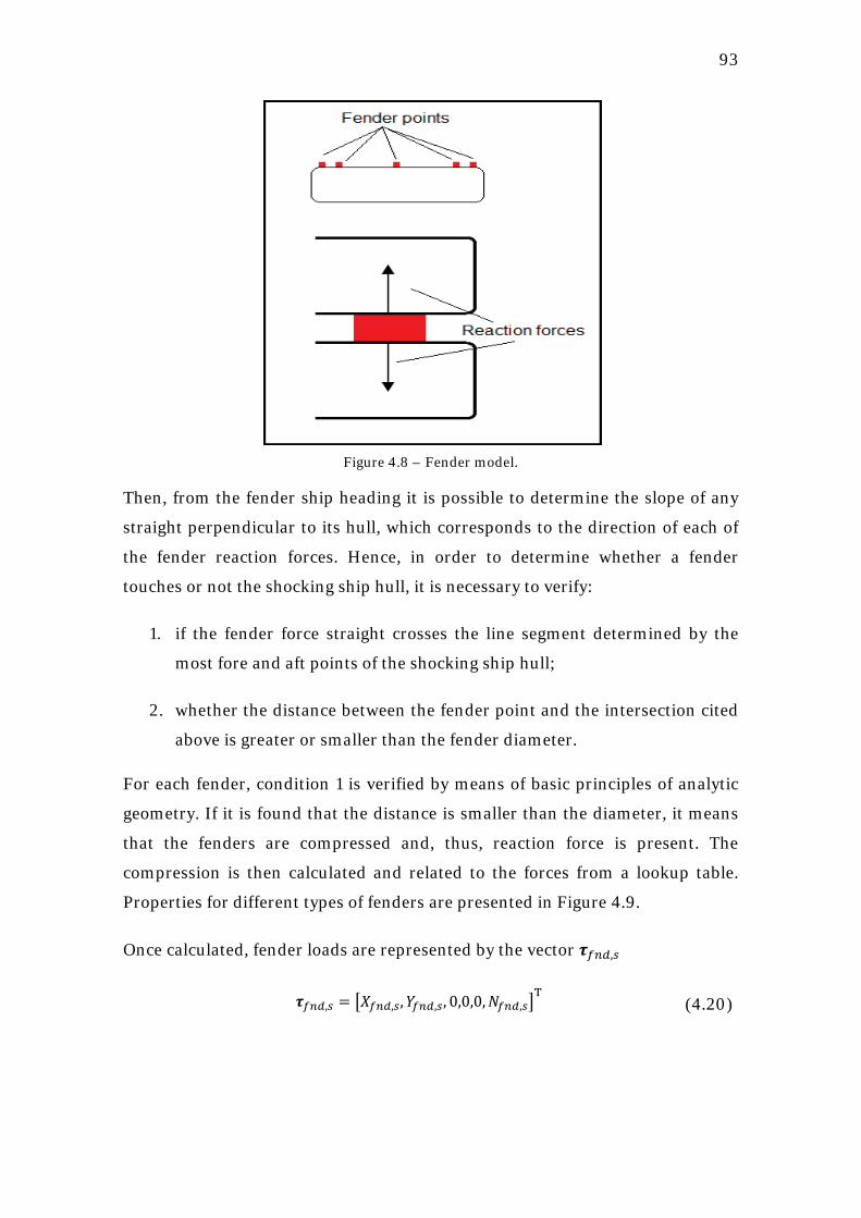
93

Figure 4.8 – Fender model.

Then, from the fender ship heading it is possible to determine the slope of any

straight perpendicular to its hull, which corresponds to the direction of each of

the fender reaction forces. Hence, in order to determine whether a fender

touches or not the shocking ship hull, it is necessary to verify:

1. if the fender force straight crosses the line segment determined by the

most fore and aft points of the shocking ship hull;

2. whether the distance between the fender point and the intersection cited

above is greater or smaller than the fender diameter.

For each fender, condition 1 is verified by means of basic principles of analytic

geometry. If it is found that the distance is smaller than the diameter, it means

that the fenders are compressed and, thus, reaction force is present. The

compression is then calculated and related to the forces from a lookup table.

Properties for different types of fenders are presented in Figure 4.9.

Once calculated, fender loads are represented by the vector 𝝉𝑓𝑛𝑑,𝑠

𝝉𝑓𝑛𝑑,𝑠 = �𝑋𝑓𝑛𝑑,𝑠,𝑌𝑓𝑛𝑑,𝑠, 0,0,0,𝑁𝑓𝑛𝑑,𝑠�T (4.20)

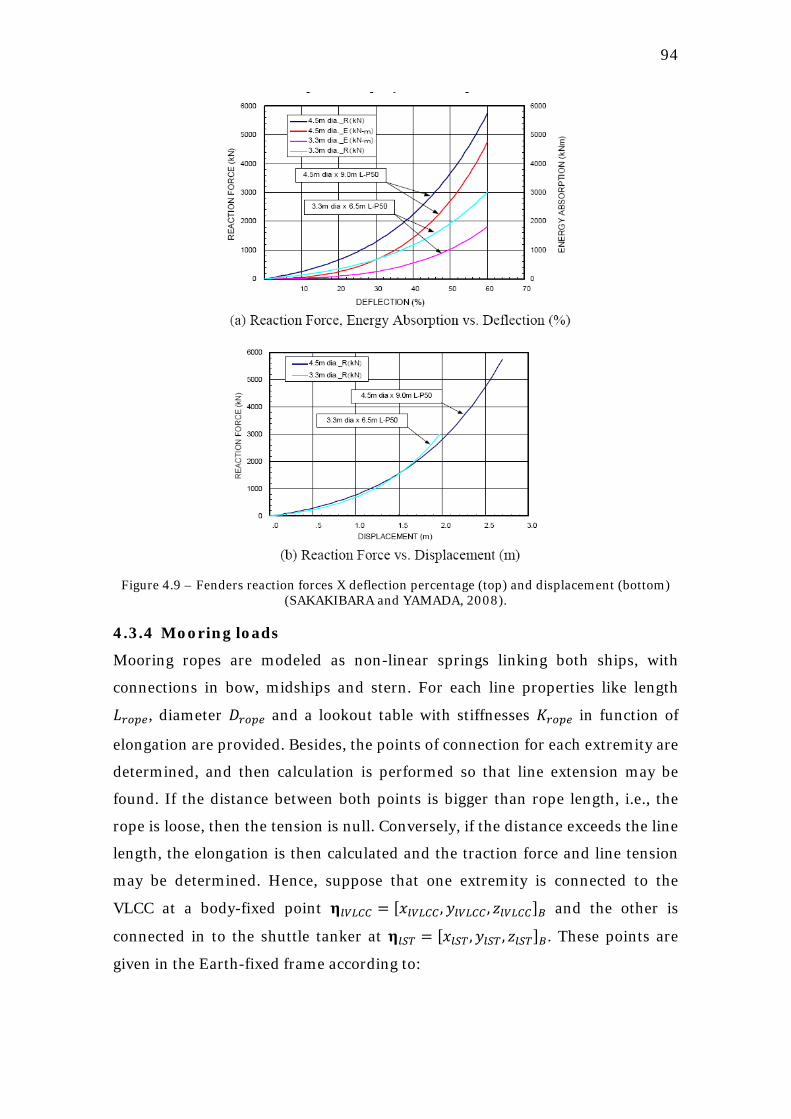
94

Figure 4.9 – Fenders reaction forces X deflection percentage (top) and displacement (bottom)

(SAKAKIBARA and YAMADA, 2008).

4.3.4 Mooring loads

Mooring ropes are modeled as non-linear springs linking both ships, with

connections in bow, midships and stern. For each line properties like length

𝐿𝑟𝑜𝑝𝑒, diameter 𝐷𝑟𝑜𝑝𝑒 and a lookout table with stiffnesses 𝐾𝑟𝑜𝑝𝑒 in function of

elongation are provided. Besides, the points of connection for each extremity are

determined, and then calculation is performed so that line extension may be

found. If the distance between both points is bigger than rope length, i.e., the

rope is loose, then the tension is null. Conversely, if the distance exceeds the line

length, the elongation is then calculated and the traction force and line tension

may be determined. Hence, suppose that one extremity is connected to the

VLCC at a body-fixed point 𝛈𝑙𝑉𝐿𝐶𝐶 = [𝑥𝑙𝑉𝐿𝐶𝐶 , 𝑦𝑙𝑉𝐿𝐶𝐶 , 𝑧𝑙𝑉𝐿𝐶𝐶]𝐵 and the other is

connected in to the shuttle tanker at 𝛈𝑙𝑆𝑇 = [𝑥𝑙𝑆𝑇 ,𝑦𝑙𝑆𝑇 , 𝑧𝑙𝑆𝑇]𝐵. These points are

given in the Earth-fixed frame according to:

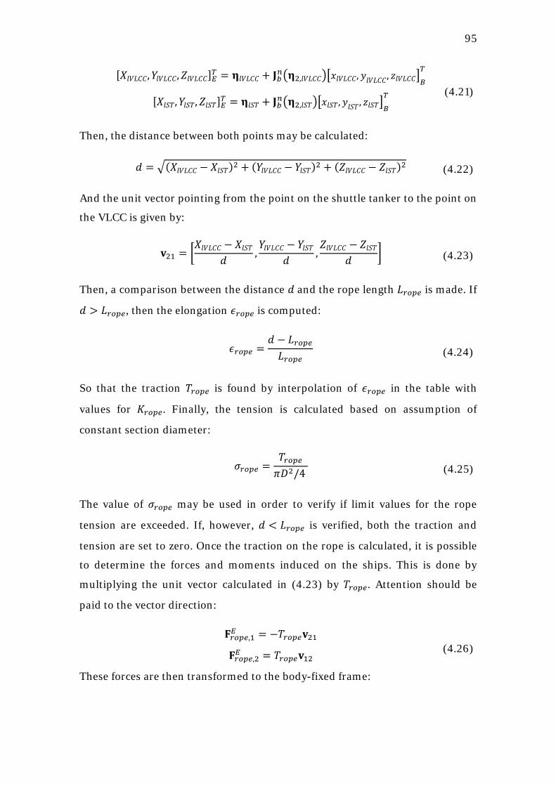
95

[𝑋𝑙𝑉𝐿𝐶𝐶,𝑌𝑙𝑉𝐿𝐶𝐶,𝑍𝑙𝑉𝐿𝐶𝐶]𝐸𝑇 = 𝛈𝑙𝑉𝐿𝐶𝐶 + 𝐉𝑏𝑛�𝛈2,𝑙𝑉𝐿𝐶𝐶��𝑥𝑙𝑉𝐿𝐶𝐶, 𝑦𝑙𝑉𝐿𝐶𝐶, 𝑧𝑙𝑉𝐿𝐶𝐶�𝐵

𝑇

[𝑋𝑙𝑆𝑇,𝑌𝑙𝑆𝑇,𝑍𝑙𝑆𝑇]𝐸𝑇 = 𝛈𝑙𝑆𝑇 + 𝐉𝑏𝑛�𝛈2,𝑙𝑆𝑇��𝑥𝑙𝑆𝑇,𝑦𝑙𝑆𝑇, 𝑧𝑙𝑆𝑇�𝐵𝑇

(4.21)

Then, the distance between both points may be calculated:

𝑑 = �(𝑋𝑙𝑉𝐿𝐶𝐶 − 𝑋𝑙𝑆𝑇)2 + (𝑌𝑙𝑉𝐿𝐶𝐶 − 𝑌𝑙𝑆𝑇)2 + (𝑍𝑙𝑉𝐿𝐶𝐶 − 𝑍𝑙𝑆𝑇)2 (4.22)

And the unit vector pointing from the point on the shuttle tanker to the point on

the VLCC is given by:

𝐯21 = �𝑋𝑙𝑉𝐿𝐶𝐶 − 𝑋𝑙𝑆𝑇

𝑑,𝑌𝑙𝑉𝐿𝐶𝐶 − 𝑌𝑙𝑆𝑇

𝑑,𝑍𝑙𝑉𝐿𝐶𝐶 − 𝑍𝑙𝑆𝑇

𝑑� (4.23)

Then, a comparison between the distance 𝑑 and the rope length 𝐿𝑟𝑜𝑝𝑒 is made. If

𝑑 > 𝐿𝑟𝑜𝑝𝑒, then the elongation 𝜖𝑟𝑜𝑝𝑒 is computed:

𝜖𝑟𝑜𝑝𝑒 =𝑑 − 𝐿𝑟𝑜𝑝𝑒𝐿𝑟𝑜𝑝𝑒

(4.24)

So that the traction 𝑇𝑟𝑜𝑝𝑒 is found by interpolation of 𝜖𝑟𝑜𝑝𝑒 in the table with

values for 𝐾𝑟𝑜𝑝𝑒. Finally, the tension is calculated based on assumption of

constant section diameter:

𝜎𝑟𝑜𝑝𝑒 =𝑇𝑟𝑜𝑝𝑒𝜋𝐷2/4

(4.25)

The value of 𝜎𝑟𝑜𝑝𝑒 may be used in order to verify if limit values for the rope

tension are exceeded. If, however, 𝑑 < 𝐿𝑟𝑜𝑝𝑒 is verified, both the traction and

tension are set to zero. Once the traction on the rope is calculated, it is possible

to determine the forces and moments induced on the ships. This is done by

multiplying the unit vector calculated in (4.23) by 𝑇𝑟𝑜𝑝𝑒. Attention should be

paid to the vector direction:

𝐅𝑟𝑜𝑝𝑒,1𝐸 = −𝑇𝑟𝑜𝑝𝑒𝐯21

𝐅𝑟𝑜𝑝𝑒,2𝐸 = 𝑇𝑟𝑜𝑝𝑒𝐯12 (4.26)

These forces are then transformed to the body-fixed frame:

96

𝐅𝑟𝑜𝑝𝑒,1𝐵 = 𝐉𝑏𝑛�𝛈2,𝑉𝐿𝐶𝐶�

−1𝐅𝑟𝑜𝑝𝑒,1𝐸

𝐅𝑟𝑜𝑝𝑒,2𝐵 = 𝐉𝑏𝑛�𝛈2,𝑆𝑇�

−1𝐅𝑟𝑜𝑝𝑒,2𝐸

(4.27)

So that the 𝑋𝑟𝑜𝑝𝑒, 𝑌𝑟𝑜𝑝𝑒, and 𝑍𝑟𝑜𝑝𝑒, components are easily determined from

𝐅𝑟𝑜𝑝𝑒,1𝐵 and 𝐅𝑟𝑜𝑝𝑒,2

𝐵 . The moment 𝐌 of a force 𝐅 applied at a distance 𝐫 from the

CG is given by:

𝐌 = 𝐫 × 𝐅 = 𝐒(𝐅)T𝐫 (4.28)

with the skew-symmetric matrix S as defined in equation (2.8). Admitting that

the body-fixed frame is placed in the centers of gravity of each ship, the moment

components 𝐾𝑟𝑜𝑝𝑒 , 𝑀𝑟𝑜𝑝𝑒 and 𝑁𝑟𝑜𝑝𝑒 are given by:

𝐾𝑟𝑜𝑝𝑒 = 𝑌𝑙1𝐹𝑟𝑜𝑝𝑒𝑍 − 𝑍𝑙1𝐹𝑟𝑜𝑝𝑒𝑌 (4.29)

𝑀𝑟𝑜𝑝𝑒 = 𝑍𝑙1𝐹𝑟𝑜𝑝𝑒𝑋 − 𝑋𝑙1𝐹𝑟𝑜𝑝𝑒𝑍 (4.30)

𝑁𝑟𝑜𝑝𝑒 = 𝑋𝑙1𝐹𝑟𝑜𝑝𝑒𝑌 − 𝑌𝑙1𝐹𝑟𝑜𝑝𝑒𝑋 (4.31)

This procedure is performed for each ship, so that the forces and moments due

to mooring lines in 6 DOF are represented by the following vector:

𝝉𝑚𝑟𝑛,𝑠 = �𝑋𝑟𝑜𝑝𝑒,𝑠,𝑌𝑟𝑜𝑝𝑒,𝑠,𝑁𝑟𝑜𝑝𝑒,𝑠,𝐾𝑟𝑜𝑝𝑒 ,𝑀𝑟𝑜𝑝𝑒 ,𝑁𝑟𝑜𝑝𝑒�T (4.32)

4.3.5 Environmental loads

Environmental action was considered with the models presented in section 2.6.

A power-spectrum for 1st-order wave loads is calculated from the FTF and the

wave spectrum, and inverse Fourier transform is used for time-domain

realization in 6 DOF, leading to the generalized forces 𝑋𝑖𝑊𝐹 (𝑖 = 1, … ,6). Also,

the mean-drift 𝐹𝑖𝑀𝐷 loads are calculated according to equation (2.83).

Wind loads (𝑋𝑤𝑖𝑛𝑑, 𝑌𝑤𝑖𝑛𝑑, 𝑁𝑤𝑖𝑛𝑑) are calculated for both ships using equations

(2.87). Although shadow effects would be significant for the case of two parallel

ships, no models were found in the literature other than CFD-based approaches,

specific for their respective situations like e.g. tandem configuration.

Finally, it is worth making a brief discussion on the method adopted for

evaluation of viscous effects. Fossen (2005) proposed to consider linear

97

components by placing the correspondent coefficients together with potential

damping in the equations of motions, while non-linear terms were included in a

separate vector. In this case, current loads could be taken into account by simply

considering the relative fluid velocity in the viscous terms, as proposed in

section 2.5.2.

This approach, however, is not adequate for the present case for two reasons.

Firstly, the available hydrodynamic derivatives model (the one adopted in

Chapter 5) was developed for the case of a single ship, and it is not known how

satisfactory it would be to use the same coefficients for the side-by-side case.

Second, it is not trivial to interpret the meaning of each term in a hydrodynamic

derivatives model. That is, one may not for example infer that a term

proportional to the acceleration corresponds to the added mass, since radiation

loads might be “hidden” into other components. Meanwhile, the formulation

presented in this section demands a clear distinction between potential and

viscous effects, so that the former should rather be determined by a trustworthy

method, like e.g. a potential theory based hydrodynamic solver.

Therefore, choice was made for the short-wing theory model of section (2.6.3)

for representation of viscous loads. This option is not free of caveats, since such

model was also developed for the single ship case. Besides, it is not adequate for

small current incidence angles, so that it was decided to disregard current in the

simulations. The situation of ships advancing in a straight path, however,

resembles to the case of static vessels with 180° incidence angle current. The

Froude number involved 𝐹𝑛 ≅ 0.05 is, on the other hand, low enough for

adoption of this model for calculation of 𝑋𝑐𝑢𝑟𝑟, 𝑌𝑐𝑢𝑟𝑟 and 𝑁𝑐𝑢𝑟𝑟.

All the above loads are combined for their respective degrees of freedom,

leading to the environmental loads vector 𝝉𝑒𝑛𝑣,𝑠.

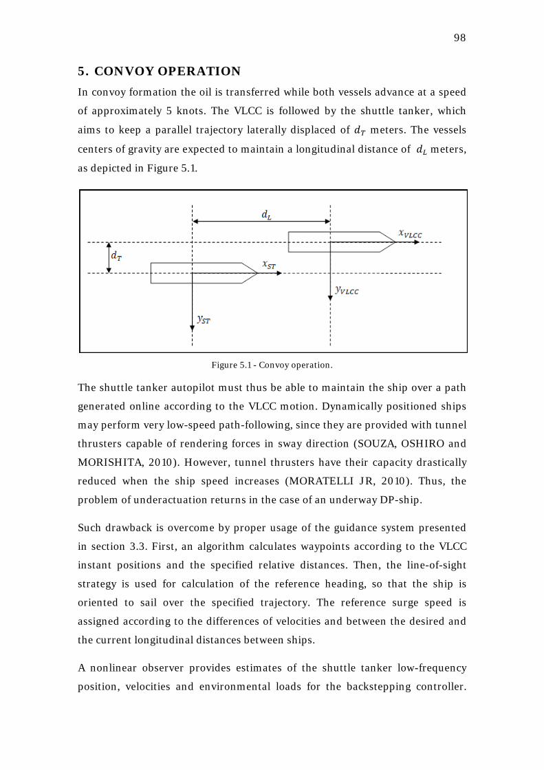
98

5. CONVOY OPERATION In convoy formation the oil is transferred while both vessels advance at a speed

of approximately 5 knots. The VLCC is followed by the shuttle tanker, which

aims to keep a parallel trajectory laterally displaced of 𝑑𝑇 meters. The vessels

centers of gravity are expected to maintain a longitudinal distance of 𝑑𝐿 meters,

as depicted in Figure 5.1.

Figure 5.1 - Convoy operation.

The shuttle tanker autopilot must thus be able to maintain the ship over a path

generated online according to the VLCC motion. Dynamically positioned ships

may perform very low-speed path-following, since they are provided with tunnel

thrusters capable of rendering forces in sway direction (SOUZA, OSHIRO and

MORISHITA, 2010). However, tunnel thrusters have their capacity drastically

reduced when the ship speed increases (MORATELLI JR, 2010). Thus, the

problem of underactuation returns in the case of an underway DP-ship.

Such drawback is overcome by proper usage of the guidance system presented

in section 3.3. First, an algorithm calculates waypoints according to the VLCC

instant positions and the specified relative distances. Then, the line-of-sight

strategy is used for calculation of the reference heading, so that the ship is

oriented to sail over the specified trajectory. The reference surge speed is

assigned according to the differences of velocities and between the desired and

the current longitudinal distances between ships.

A nonlinear observer provides estimates of the shuttle tanker low-frequency

position, velocities and environmental loads for the backstepping controller.

99

Such controller is also fed with the references generated by the guidance system,

determining the surge force and yaw moments necessary to make the shuttle

tanker to follow the waypoints. The resultant commanded loads are limited by

models that represent the actuator dynamics. For the force surge, this is done by

simply bounding the maximum and minimum thrust that a common Suezmax

propeller is able to provide. For yaw moment, a rather developed formulation

calculates rudder deflection departing from the commanded moment and

rudder dimensions data.

Both the VLCC and the shuttle tanker dynamics are formulated according to a

maneuvering model based on hydrodynamic derivatives determined in PMM

tests for a tanker. Such tests were performed in the DMI towing tank, in the city

of Lyngby, Denmark.

5.1 DYNAMICS

Unlike the side-by-side case, ships motions in the convoy operation may be

accurately represented by the superposition of low- and wave-frequency signals

provided by a maneuvering and a seakeeping model, respectively. Also, only

horizontal motions are of interest for this operation, such that a formulation in

3 DOF is adequate for the purposes of this study.

Both the Earth-fixed and body-fixed coordinate systems are used to describe the

equations of motions. Then, let the maneuvering model of section 2.7.1 in 3 DOF

be described according to (PEREZ and BLANKE, 2008):

�̇� = 𝐉(𝜓)𝛎 (5.1)

𝐌𝑅𝐵 = 𝛕 − 𝐂𝑅𝐵(𝛎) (5.2)

with the state vectors 𝛈 = [𝑥, 𝑦,𝜓]T and 𝛎 = [𝑢, 𝑣, 𝑟]T correspondent to

horizontal motions, only. The Coriolis and centripetal matrix 𝐂𝑅𝐵(𝛎) is given by:

𝐂𝑅𝐵(𝛎) = �0 0 −𝑚(𝑥𝑔𝑟 + 𝑣)0 0 𝑚𝑢

𝑚(𝑥𝑔𝑟 + 𝑣) −𝑚𝑢 0� (5.3)

100

where 𝑚 is the ship mass and 𝑥𝑔 is the distance of the center of gravity from the

body-fixed coordinate system origin. The vector 𝛕 is a sum of hydrodynamic,

control and environmental loads components, that is:

𝛕 = 𝛕ℎ𝑖𝑑 + 𝛕𝑐𝑡𝑟 + 𝛕𝑒𝑛𝑣 (5.4)

with 𝛕ℎ𝑖𝑑 = 𝛕ℎ𝑖𝑑(�̇�𝑟, 𝛎𝑟 ,𝛈) composed by forces and moments due to potential and

viscous effects, calculated by means of coefficients obtained in PMM tests

(FORCE TECHNOLOGY, 2002). The 𝛕𝑒𝑛𝑣 vector consists of loads from wind

and mean drift effects from waves, calculated as presented in section 2.6.

5.2 CONTROL

The control system comprises a combination of a reference generator, a

nonlinear observer and a backstepping controller designed for the autopilot

case. Such subsystems are described in the following subsections.

5.2.1 References generator (shuttle tanker)

Surge velocity

Let the VLCC sail with at a speed of 𝑈𝑉𝐿𝐶𝐶 m/s and at a distance of 𝑑𝐿 meters

forward from the shuttle tanker (Figure 5.1). For a given desired longitudinal

distance 𝑑𝐿,𝑟𝑒𝑓, the shuttle tanker reference surge speed 𝑢𝑆𝑇,𝑟𝑒𝑓 is then calculated

according to:

𝑢𝑆𝑇,𝑟𝑒𝑓 =𝑈𝑉𝐿𝐶𝐶 + 𝑘(𝑑𝐿 − 𝑑𝐿,𝑟𝑒𝑓)

cos𝜓𝑟𝑒𝑙 (5.5)

where 𝑘 is a positive gain and 𝜓𝑟𝑒𝑙 is the difference between the headings of the

VLCC and the shuttle tanker:

𝜓𝑟𝑒𝑓 = 𝜓𝑉𝐿𝐶𝐶 − 𝜓𝑆𝑇 (5.6)

The division by cos𝜓𝑟𝑒𝑙 offsets the fact the ships trajectories are not perfectly

parallel. According to the formulation above, the shuttle tanker surge velocity is

assigned in order to keep the reference longitudinal distance 𝑑𝐿 between both

ships. When the error is positive, that is, ships are farther than desired, the

shuttle tanker speeds up in order to approximate itself to the VLCC. Oppositely,

101

the reference speed decreases. The gain 𝑘 should be adjusted in order to specify

the speed change rate.

Waypoints generator

The line-of-sight strategy presented in section (3.3) demands waypoints in order

to properly guide the ship through the desired trajectory. In the present case,

such waypoints are generated according to the VLCC position and the specified

lateral distance between ships trajectories. A circle of acceptance with center in

each waypoint and a given radius 𝑟𝑤𝑝 determines the region the shuttle tanker

must enter in order to the waypoint to be considered the current waypoint.

Once it happens, the next waypoint is generated according to the following

expression:

�𝑋𝑤𝑝,𝑛𝑥𝑡𝑌𝑤𝑝,𝑛𝑥𝑡

� = �𝑋𝑡𝑟𝑎𝑗𝑌𝑡𝑟𝑎𝑗

� + 𝑑𝑤𝑝 �cos𝜓𝑉𝐿𝐶𝐶sin𝜓𝑉𝐿𝐶𝐶

� (5.7)

where 𝑑𝑤𝑝 is the distance between the next waypoint position and the shuttle

tanker desired position �𝑋𝑡𝑟𝑎𝑗,𝑌𝑡𝑟𝑎𝑗�T

, calculated according to:

�𝑋𝑡𝑟𝑎𝑗𝑌𝑡𝑟𝑎𝑗

� = �𝑥𝑣𝑙𝑐𝑐𝑦𝑣𝑙𝑐𝑐� + �cos𝜓𝑉𝐿𝐶𝐶 − sin𝜓𝑉𝐿𝐶𝐶

sin𝜓𝑉𝐿𝐶𝐶 cos𝜓𝑉𝐿𝐶𝐶� �−𝑑𝐿,𝑟𝑒𝑓𝑑𝑇

� (5.8)

with 𝑥𝑣𝑙𝑐𝑐, 𝑦𝑣𝑙𝑐𝑐, 𝜓𝑣𝑙𝑐𝑐, 𝑑𝐿,𝑟𝑒𝑓 and 𝑑𝑇 as defined in Figure 5.1. Given two

consecutive waypoints and the estimated current shuttle tanker position, the

desired heading 𝜓𝑆𝑇,𝑟𝑒𝑓 is determined by:

𝜓𝑆𝑇,𝑟𝑒𝑓 = atan �𝑦𝑙𝑜𝑠 − 𝑦�𝑆𝑇𝑥𝑙𝑜𝑠 − �̅�𝑆𝑇

� (5.9)

with 𝑥𝑙𝑜𝑠 and 𝑦𝑙𝑜𝑠 determined according to the procedure described on section

3.3 and �̅�𝑆𝑇 and 𝑦�𝑆𝑇 estimated by the state observer.

5.2.2 Controllers

VLCC

The VLCC autopilot calculates the control loads according to the procedure

detailed in section 3.1.1. The references for surge velocity 𝑢𝑉𝐿𝐶𝐶,𝑟𝑒𝑓 and heading

𝜓𝑉𝐿𝐶𝐶,𝑟𝑒𝑓 are manually determined, since the task for this ship is simply to

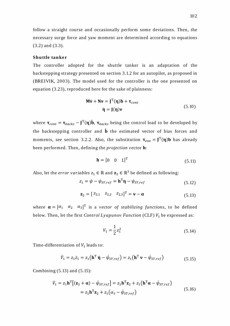
102

follow a straight course and occasionally perform some deviations. Then, the

necessary surge force and yaw moment are determined according to equations

(3.2) and (3.3).

Shuttle tanker

The controller adopted for the shuttle tanker is an adaptation of the

backstepping strategy presented on section 3.1.2 for an autopilot, as proposed in

(BREIVIK, 2003). The model used for the controller is the one presented on

equation (3.23), reproduced here for the sake of plainness:

𝐌�̇� + 𝐍𝛎 = 𝐉T(𝛈)𝐛 + 𝛕𝑐𝑜𝑛𝑡

�̇� = 𝐉(𝛈)𝛎 (5.10)

where 𝛕𝑐𝑜𝑛𝑡 = 𝛕𝑏𝑎𝑐𝑘𝑠 − 𝐉T(𝛈)�̂�, 𝛕𝑏𝑎𝑐𝑘𝑠 being the control load to be developed by

the backstepping controller and �̂� the estimated vector of bias forces and

moments, see section 3.2.2. Also, the substitution 𝛕𝑒𝑛𝑣 = 𝐉T(𝛈)𝐛 has already

been performed. Then, defining the projection vector 𝐡:

𝐡 = [0 0 1]T (5.11)

Also, let the error variables 𝑧1 ∈ ℝ and 𝐳2 ∈ ℝ3 be defined as following:

𝑧1 = 𝜓 − 𝜓𝑆𝑇,𝑟𝑒𝑓 = 𝐡T𝛈 − 𝜓𝑆𝑇,𝑟𝑒𝑓 (5.12)

𝐳2 = [ 𝑧2,1 𝑧2,2 𝑧2,3]T = 𝛎 − 𝛂 (5.13)

where 𝛂 = [𝛼1 𝛼2 𝛼3]T is a vector of stabilizing functions, to be defined

below. Then, let the first Control Lyapunov Function (CLF) 𝑉1 be expressed as:

𝑉1 =12𝑧12 (5.14)

Time-differentiation of 𝑉1 leads to:

�̇�1 = 𝑧1�̇�1 = 𝑧1�𝐡T �̇� − �̇�𝑆𝑇,𝑟𝑒𝑓� = 𝑧1�𝐡T 𝛎 − �̇�𝑆𝑇,𝑟𝑒𝑓� (5.15)

Combining (5.13) and (5.15):

�̇�1 = 𝑧1𝐡T�(𝐳2 + 𝛂) − �̇�𝑆𝑇,𝑟𝑒𝑓� = 𝑧1𝐡T𝐳2 + 𝑧1�𝐡T𝛂 − �̇�𝑆𝑇,𝑟𝑒𝑓�

= 𝑧1𝐡T𝐳2 + 𝑧1�𝛼3 − �̇�𝑆𝑇,𝑟𝑒𝑓� (5.16)

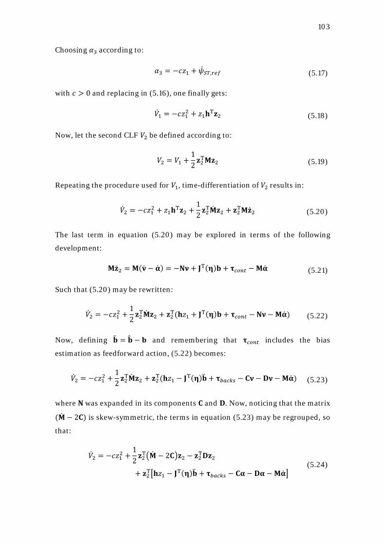
103

Choosing 𝛼3 according to:

𝛼3 = −𝑐𝑧1 + �̇�𝑆𝑇,𝑟𝑒𝑓 (5.17)

with 𝑐 > 0 and replacing in (5.16), one finally gets:

�̇�1 = −𝑐𝑧12 + 𝑧1𝐡T𝐳2 (5.18)

Now, let the second CLF 𝑉2 be defined according to:

𝑉2 = 𝑉1 +12𝐳2T𝐌𝐳2 (5.19)

Repeating the procedure used for 𝑉1, time-differentiation of 𝑉2 results in:

�̇�2 = −𝑐𝑧12 + 𝑧1𝐡T𝐳2 +12𝐳2T�̇�𝐳2 + 𝐳2T𝐌�̇�2 (5.20)

The last term in equation (5.20) may be explored in terms of the following

development:

𝐌�̇�2 = 𝐌(�̇� − �̇�) = −𝐍𝛎 + 𝐉T(𝛈)𝐛 + 𝛕𝑐𝑜𝑛𝑡 − 𝐌�̇� (5.21)

Such that (5.20) may be rewritten:

�̇�2 = −𝑐𝑧12 +12𝐳2T�̇�𝐳2 + 𝐳2T(𝐡𝑧1 + 𝐉T(𝛈)𝐛 + 𝛕𝑐𝑜𝑛𝑡 − 𝐍𝛎 −𝐌�̇�) (5.22)

Now, defining �̅� = �̂� − 𝐛 and remembering that 𝛕𝑐𝑜𝑛𝑡 includes the bias

estimation as feedforward action, (5.22) becomes:

�̇�2 = −𝑐𝑧12 +12𝐳2T�̇�𝐳2 + 𝐳2T(𝐡𝑧1 − 𝐉T(𝛈)�̅� + 𝛕𝑏𝑎𝑐𝑘𝑠 − 𝐂𝛎 − 𝐃𝛎 −𝐌�̇�) (5.23)

where 𝐍 was expanded in its components 𝐂 and 𝐃. Now, noticing that the matrix

(�̇� − 2𝐂) is skew-symmetric, the terms in equation (5.23) may be regrouped, so

that:

�̇�2 = −𝑐𝑧12 +

12𝐳2T��̇� − 2𝐂�𝐳2 − 𝐳2T𝐃𝐳2

+ 𝐳2T�𝐡𝑧1 − 𝐉T(𝛈)�̅� + 𝛕𝑏𝑎𝑐𝑘𝑠 − 𝐂𝛂 − 𝐃𝛂 −𝐌�̇�� (5.24)

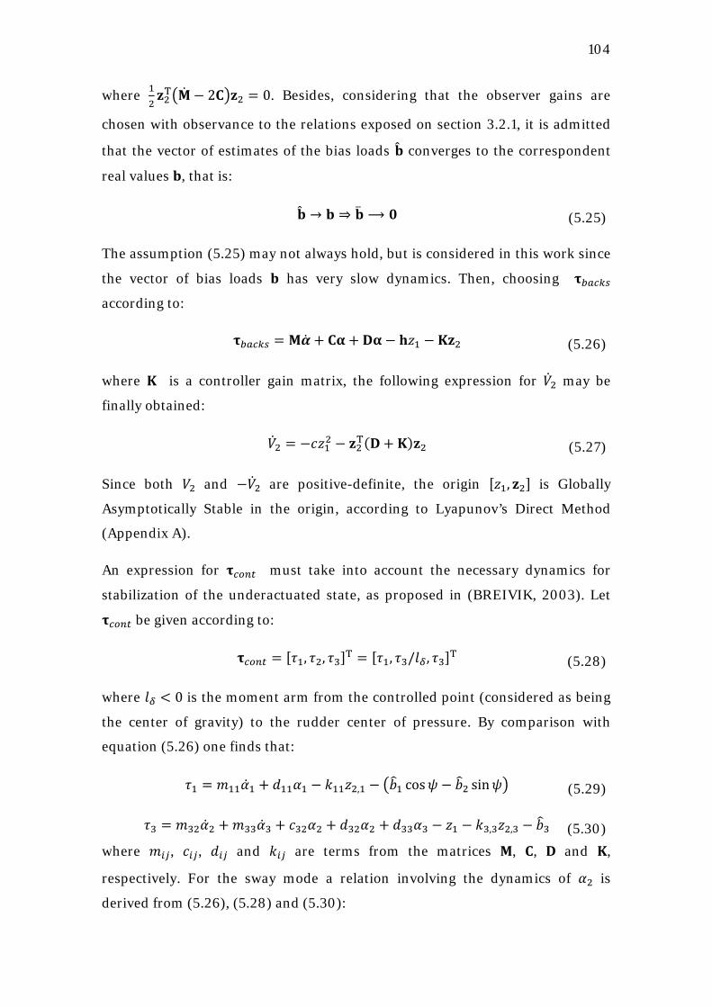
104

where 12𝐳2T��̇� − 2𝐂�𝐳2 = 0. Besides, considering that the observer gains are

chosen with observance to the relations exposed on section 3.2.1, it is admitted

that the vector of estimates of the bias loads �̂� converges to the correspondent

real values 𝐛, that is:

�̂� → 𝐛 ⇒ �̅� ⟶ 𝟎 (5.25)

The assumption (5.25) may not always hold, but is considered in this work since

the vector of bias loads 𝐛 has very slow dynamics. Then, choosing 𝛕𝑏𝑎𝑐𝑘𝑠

according to:

𝛕𝑏𝑎𝑐𝑘𝑠 = 𝐌�̇� + 𝐂𝛂 + 𝐃𝛂 − 𝐡𝑧1 − 𝐊𝐳2 (5.26)

where 𝐊 is a controller gain matrix, the following expression for �̇�2 may be

finally obtained:

�̇�2 = −𝑐𝑧12 − 𝐳2T(𝐃 + 𝐊)𝐳2 (5.27)

Since both 𝑉2 and −�̇�2 are positive-definite, the origin [𝑧1, 𝐳2] is Globally

Asymptotically Stable in the origin, according to Lyapunov’s Direct Method

(Appendix A).

An expression for 𝛕𝑐𝑜𝑛𝑡 must take into account the necessary dynamics for

stabilization of the underactuated state, as proposed in (BREIVIK, 2003). Let

𝛕𝑐𝑜𝑛𝑡 be given according to:

𝛕𝑐𝑜𝑛𝑡 = [𝜏1, 𝜏2, 𝜏3]T = [𝜏1, 𝜏3/𝑙𝛿 , 𝜏3]T (5.28)

where 𝑙𝛿 < 0 is the moment arm from the controlled point (considered as being

the center of gravity) to the rudder center of pressure. By comparison with

equation (5.26) one finds that:

𝜏1 = 𝑚11�̇�1 + 𝑑11𝛼1 − 𝑘11𝑧2,1 − �𝑏�1 cos𝜓 − 𝑏�2 sin𝜓� (5.29)

𝜏3 = 𝑚32�̇�2 + 𝑚33�̇�3 + 𝑐32𝛼2 + 𝑑32𝛼2 + 𝑑33𝛼3 − 𝑧1 − 𝑘3,3𝑧2,3 − 𝑏�3 (5.30) where 𝑚𝑖𝑗, 𝑐𝑖𝑗, 𝑑𝑖𝑗 and 𝑘𝑖𝑗 are terms from the matrices 𝐌, 𝐂, 𝐃 and 𝐊,

respectively. For the sway mode a relation involving the dynamics of 𝛼2 is

derived from (5.26), (5.28) and (5.30):

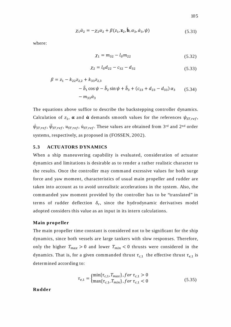
105

𝜒1�̇�2 = −𝜒2𝛼2 + 𝛽(𝑧1, 𝐳2, �̂�,𝛼3, �̇�3,𝜓) (5.31)

where:

𝜒1 = 𝑚32 − 𝑙𝛿𝑚22 (5.32)

𝜒2 = 𝑙𝛿𝑑22 − 𝑐32 − 𝑑32 (5.33)

𝛽 = 𝑧1 − 𝑘22𝑧2,2 + 𝑘33𝑧2,3

− 𝑏�1 cos𝜓 − 𝑏�2 sin𝜓 + 𝑏�3 + (𝑐23 + 𝑑23 − 𝑑33)𝛼3− 𝑚33�̇�3

(5.34)

The equations above suffice to describe the backstepping controller dynamics.

Calculation of 𝑧1, 𝛂 and �̇� demands smooth values for the references 𝜓𝑆𝑇,𝑟𝑒𝑓,

�̇�𝑆𝑇,𝑟𝑒𝑓, �̈�𝑆𝑇,𝑟𝑒𝑓, 𝑢𝑆𝑇,𝑟𝑒𝑓, �̇�𝑆𝑇,𝑟𝑒𝑓. These values are obtained from 3rd and 2nd order

systems, respectively, as proposed in (FOSSEN, 2002).

5.3 ACTUATORS DYNAMICS

When a ship maneuvering capability is evaluated, consideration of actuator

dynamics and limitations is desirable as to render a rather realistic character to

the results. Once the controller may command excessive values for both surge

force and yaw moment, characteristics of usual main propeller and rudder are

taken into account as to avoid unrealistic accelerations in the system. Also, the

commanded yaw moment provided by the controller has to be “translated” in

terms of rudder deflection 𝛿𝑟, since the hydrodynamic derivatives model

adopted considers this value as an input in its intern calculations.

Main propeller

The main propeller time constant is considered not to be significant for the ship

dynamics, since both vessels are large tankers with slow responses. Therefore,

only the higher 𝑇𝑚𝑎𝑥 > 0 and lower 𝑇𝑚𝑖𝑛 < 0 thrusts were considered in the

dynamics. That is, for a given commanded thrust 𝜏𝑐,1 the effective thrust 𝜏𝑒,1 is

determined according to:

𝜏𝑒,1 = �min{𝜏𝑐,1,𝑇𝑚𝑎𝑥} ,𝑓𝑜𝑟 𝜏𝑐,1 > 0max{𝜏𝑐,1,𝑇𝑚𝑖𝑛} ,𝑓𝑜𝑟 𝜏𝑐,1 < 0

� (5.35)

Rudder

106

From the commanded yaw moment 𝜏𝑐,3 determined by the controller, the lift

force on the rudder is found according to:

𝐿𝑟𝑑𝑑 = 𝜏𝑐,3/𝑙𝛿 (5.36)

Defining the lift coefficient 𝐶𝐿 (SKEJIC, 2008):

𝐶𝐿(𝛿𝑟) = 2𝜋𝛬(𝛬 + 0.7)(𝛬 + 1.7)2 sin(𝛿𝑟) + 𝐶𝑄 sin(𝛿𝑟) |sin (𝛿𝑟)|cos (𝛿𝑟) (5.37)

where 𝐶𝑄 ≈ 1 is the resistance coefficient, the lift force be modeled according to:

𝐿𝑟𝑑𝑑 =𝜌𝑤2𝐴𝑟𝑒𝐶𝐿(𝛿𝑟)𝑢𝑟𝑑𝑑|𝑢𝑟𝑑𝑑| (5.38)

where 𝜌𝑤 is the water density and the effective rudder area 𝐴𝑟𝑒 is calculated by

means of the propeller diameter 𝐷𝑝 and mean chord 𝑐𝑚:

𝐴𝑟𝑒 ≈ 𝐷𝑝𝑐𝑚 (5.39)

and the rudder flow velocity calculated by means of the following expression:

𝑢𝑟𝑑𝑑 = 𝑢𝑟 + 𝑘𝑢 ��8

𝜋𝜌𝑤𝐷𝑝2𝑇ℎ + 𝑢𝑟2 − 𝑢𝑟� (5.40)

where 𝑇ℎ is the value of the thrust developed by the propeller and 𝑘𝑢 ≈ 0.5 is an

induced velocity coefficient. For a practical range of values for 𝛿𝑟 it may be

admitted that expression (5.37) may be approximated by a linear relation:

𝐶𝐿 ≈ 𝑐1𝛿𝑟 (5.41)

Finally, grouping constant terms of (5.37) in a new coefficient 𝐿𝛿:

𝐿𝛿 =𝜌𝑤2𝐴𝑟𝑒𝑐1 (5.42)

The rudder deflection angle may then be related to the lift force, for a given

value of 𝑢𝑟𝑑𝑑, according to:

𝛿𝑟 =𝐿𝑟𝑑𝑑

𝐿𝛿𝑢𝑟𝑑𝑑|𝑢𝑟𝑑𝑑| (5.43)

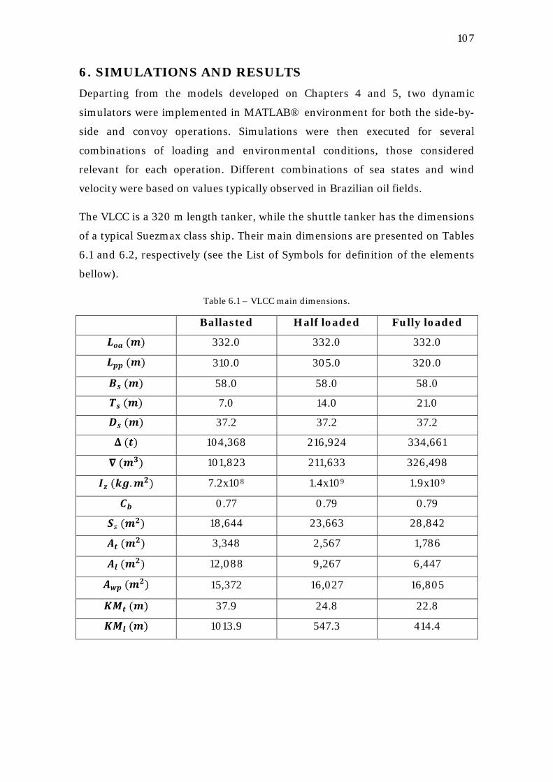
107

6. SIMULATIONS AND RESULTS Departing from the models developed on Chapters 4 and 5, two dynamic

simulators were implemented in MATLAB® environment for both the side-by-

side and convoy operations. Simulations were then executed for several

combinations of loading and environmental conditions, those considered

relevant for each operation. Different combinations of sea states and wind

velocity were based on values typically observed in Brazilian oil fields.

The VLCC is a 320 m length tanker, while the shuttle tanker has the dimensions

of a typical Suezmax class ship. Their main dimensions are presented on Tables

6.1 and 6.2, respectively (see the List of Symbols for definition of the elements

bellow).

Table 6.1 – VLCC main dimensions.

Ballasted Half loaded Fully loaded

𝑳𝒐𝒂 (𝒎) 332.0 332.0 332.0

𝑳𝒑𝒑 (𝒎) 310.0 305.0 320.0

𝑩𝒔 (𝒎) 58.0 58.0 58.0

𝑻𝒔 (𝒎) 7.0 14.0 21.0

𝑫𝒔 (𝒎) 37.2 37.2 37.2

𝚫 (𝒕) 104,368 216,924 334,661

𝛁 (𝒎𝟑) 101,823 211,633 326,498

𝑰𝒛 (𝒌𝒈.𝒎𝟐) 7.2x108 1.4x109 1.9x109

𝑪𝒃 0.77 0.79 0.79

𝑺𝑠 (𝒎𝟐) 18,644 23,663 28,842

𝑨𝒕 (𝒎𝟐) 3,348 2,567 1,786

𝑨𝒍 (𝒎𝟐) 12,088 9,267 6,447

𝑨𝒘𝒑 (𝒎𝟐) 15,372 16,027 16,805

𝑲𝑴𝒕 (𝒎) 37.9 24.8 22.8

𝑲𝑴𝒍 (𝒎) 1013.9 547.3 414.4

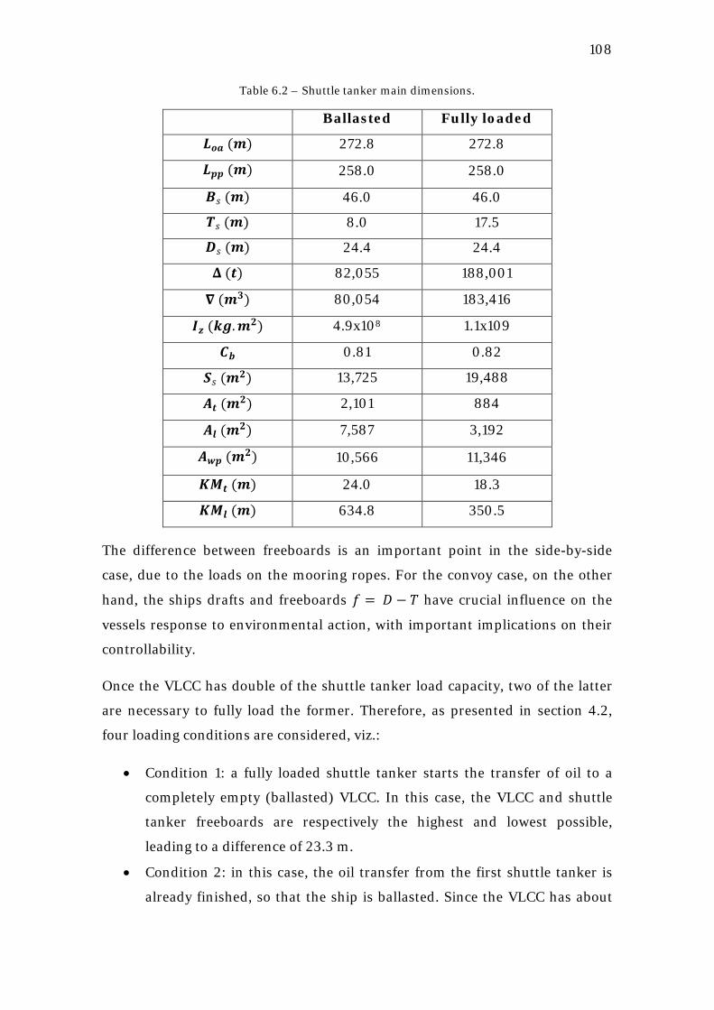
108

Table 6.2 – Shuttle tanker main dimensions.

Ballasted Fully loaded

𝑳𝒐𝒂 (𝒎) 272.8 272.8

𝑳𝒑𝒑 (𝒎) 258.0 258.0

𝑩𝑠 (𝒎) 46.0 46.0

𝑻𝑠 (𝒎) 8.0 17.5

𝑫𝑠 (𝒎) 24.4 24.4

𝚫 (𝒕) 82,055 188,001

𝛁 (𝒎𝟑) 80,054 183,416

𝑰𝒛 (𝒌𝒈.𝒎𝟐) 4.9x108 1.1x109

𝑪𝒃 0.81 0.82

𝑺𝑠 (𝒎𝟐) 13,725 19,488

𝑨𝒕 (𝒎𝟐) 2,101 884

𝑨𝒍 (𝒎𝟐) 7,587 3,192

𝑨𝒘𝒑 (𝒎𝟐) 10,566 11,346

𝑲𝑴𝒕 (𝒎) 24.0 18.3

𝑲𝑴𝒍 (𝒎) 634.8 350.5

The difference between freeboards is an important point in the side-by-side

case, due to the loads on the mooring ropes. For the convoy case, on the other

hand, the ships drafts and freeboards 𝑓 = 𝐷 − 𝑇 have crucial influence on the

vessels response to environmental action, with important implications on their

controllability.

Once the VLCC has double of the shuttle tanker load capacity, two of the latter

are necessary to fully load the former. Therefore, as presented in section 4.2,

four loading conditions are considered, viz.:

• Condition 1: a fully loaded shuttle tanker starts the transfer of oil to a

completely empty (ballasted) VLCC. In this case, the VLCC and shuttle

tanker freeboards are respectively the highest and lowest possible,

leading to a difference of 23.3 m.

• Condition 2: in this case, the oil transfer from the first shuttle tanker is

already finished, so that the ship is ballasted. Since the VLCC has about

109

twice the shuttle tanker load capacity, it gets therefore with half of its

nominal payload. The difference between freeboard decreases to 6.8 m.

• Condition 3: a second fully loaded shuttle tanker begins its transfer

process to the half loaded VLCC. The freeboards difference is again

increased, reaching 16.3 m.

• Condition 4: finally, the VLCC gets completely loaded, after having

received the total cargo of the shuttle tanker. In this case, the ships

freeboards are almost the same, with a difference of just 0.2 m.

Additional information on hydrodynamic data, environmental conditions and

more details particularly relevant for each operation are presented in their

correspondent following sections.

6.1 SIDE-BY-SIDE

For the side-by-side case, it was considered that ships should follow a straight

trajectory at 5 knots, under influence of waves and wind. The shuttle tanker was

always equipped with five fenders equally distributed along the hull, since it is

the smaller ship. Three different mooring system arrangements were tested, and

a total of 18 combinations of incidence angles, wave heights and periods were

considered. The objective was to monitor whether the loads on mooring ropes

crossed or not the acceptable values.

6.1.1 Fenders properties

Each fender was considered to have 3.3 m in diameter, and their compression

properties are displayed on Table 6.3. The value for 100% of compression is

clearly unreal, and was assigned in order to avoid “overlaps” between ships. It

was admitted that no friction took place between fenders and the ships, so that

only loads perpendicular to the hulls were considered.

6.1.2 Mooring system

According to OCIMF’s guidelines for ship-to-ship operations (OCIMF, 2005),

typical mooring arrangements consist of 6 to 8 ropes tying ships bows, 4 to 6

ropes linking the sterns and two pairs of mooring bites fore and aft the

manifolds (Figure 6.1). It is admitted that each group of mooring lines are

connected to a same point in each ship. Therefore, the considered mooring

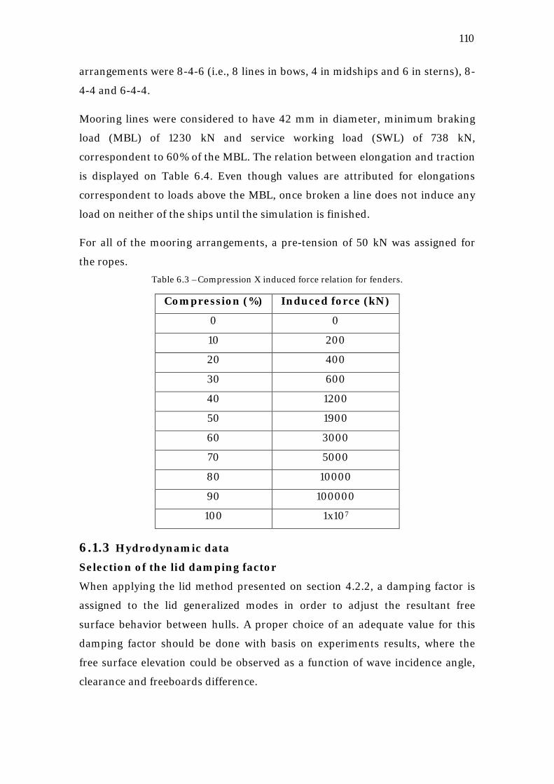
110

arrangements were 8-4-6 (i.e., 8 lines in bows, 4 in midships and 6 in sterns), 8-

4-4 and 6-4-4.

Mooring lines were considered to have 42 mm in diameter, minimum braking

load (MBL) of 1230 kN and service working load (SWL) of 738 kN,

correspondent to 60% of the MBL. The relation between elongation and traction

is displayed on Table 6.4. Even though values are attributed for elongations

correspondent to loads above the MBL, once broken a line does not induce any

load on neither of the ships until the simulation is finished.

For all of the mooring arrangements, a pre-tension of 50 kN was assigned for

the ropes. Table 6.3 –Compression X induced force relation for fenders.

Compression (%) Induced force (kN)

0 0

10 200

20 400

30 600

40 1200

50 1900

60 3000

70 5000

80 10000

90 100000

100 1x107

6.1.3 Hydrodynamic data Selection of the lid damping factor

When applying the lid method presented on section 4.2.2, a damping factor is

assigned to the lid generalized modes in order to adjust the resultant free

surface behavior between hulls. A proper choice of an adequate value for this

damping factor should be done with basis on experiments results, where the

free surface elevation could be observed as a function of wave incidence angle,

clearance and freeboards difference.

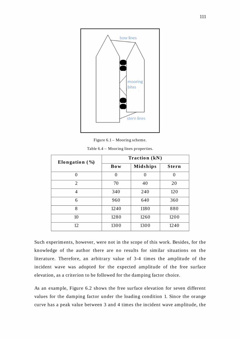
111

Figure 6.1 – Mooring scheme.

Table 6.4 – Mooring lines properties.

Elongation (%) Traction (kN)

Bow Midships Stern

0 0 0 0

2 70 40 20

4 340 240 120

6 960 640 360

8 1240 1180 880

10 1280 1260 1200

12 1300 1300 1240

Such experiments, however, were not in the scope of this work. Besides, for the

knowledge of the author there are no results for similar situations on the

literature. Therefore, an arbitrary value of 3-4 times the amplitude of the

incident wave was adopted for the expected amplitude of the free surface

elevation, as a criterion to be followed for the damping factor choice.

As an example, Figure 6.2 shows the free surface elevation for seven different

values for the damping factor under the loading condition 1. Since the orange

curve has a peak value between 3 and 4 times the incident wave amplitude, the

112

correspondent value of 3x105 kg/s was adopted. Therefore, all hydrodynamic

data used for condition 1 simulations are those obtained with this value for the

damping factor of the lid generalized modes. A similar procedure was applied

for the other loading conditions.

Figure 6.2 – Damped free surface elevation – for a unitary incident wave amplitude – for

loading condition 1. The x-axis corresponds to points distributed along the lid length, with 0 and 38 corresponding to the aft- and fore-most extremities, respectively (NYX KNOWLEDGE, 2011).

Memory functions

As discussed on Chapters 2 and 4, in side-by-side operations the mooring

system induces wave-frequency loads shared between both ships. The

implication of this phenomenon is that it becomes necessary to consider the 1st

order wave loads in the equations of motions, demanding a unified model for

maneuvering and seakeeping.

Since ships are excited, both added mass and potential damping must be

considered as frequency-dependent coefficients. However, this would lead to

time- and frequency-dependent equations of motions, a drawback that may be

overcome through substitution of frequency-dependent coefficients by

convolutions of memory functions in time domain.

This solution, however, would be much time-consuming, so that the state-space

approximation of equations (2.123) and (2.124) becomes convenient:

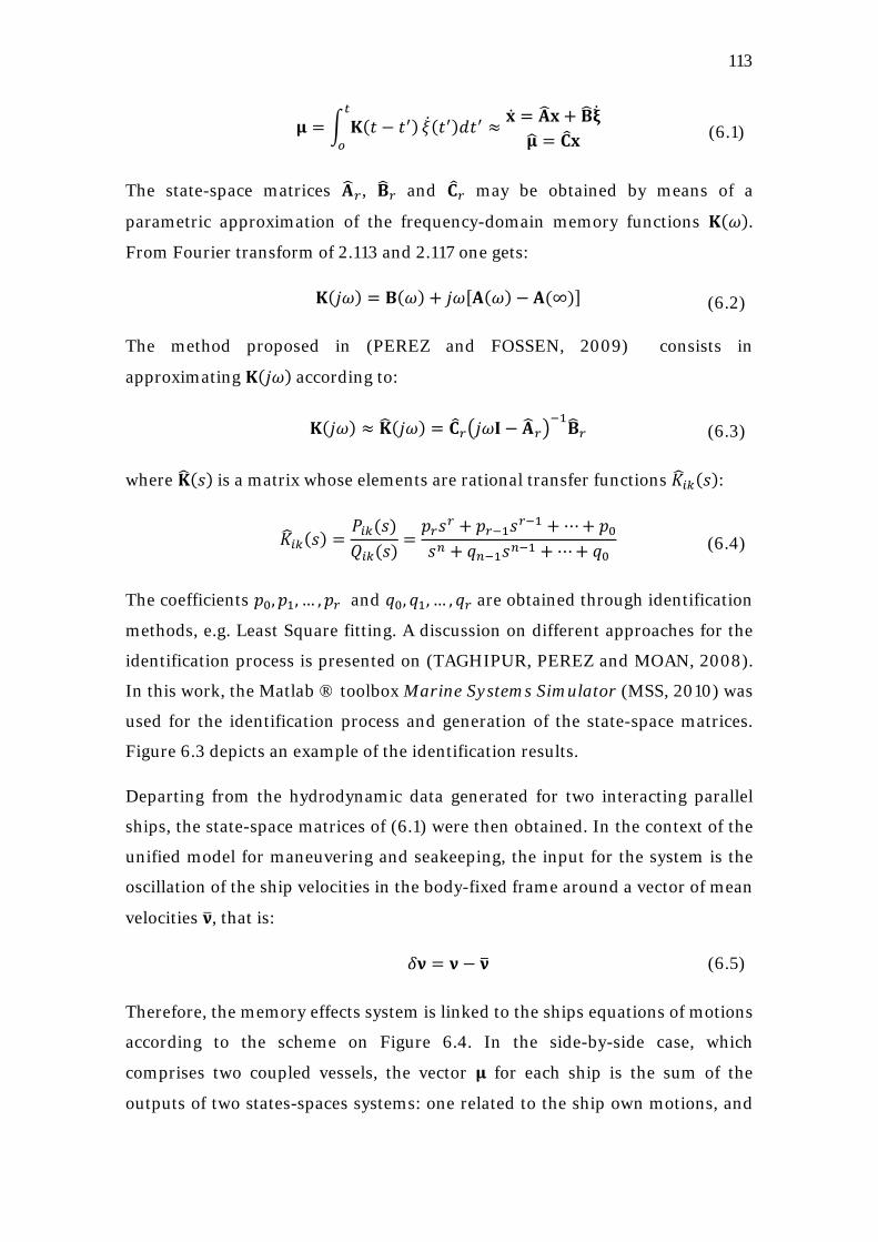
113

𝛍 = � 𝐊(𝑡 − 𝑡′)𝑡

𝑜�̇�(𝑡′)𝑑𝑡′ ≈ �̇� = 𝐀�𝐱 + 𝐁��̇�

𝛍� = 𝐂�𝐱 (6.1)

The state-space matrices 𝐀�𝑟, 𝐁�𝑟 and 𝐂�𝑟 may be obtained by means of a

parametric approximation of the frequency-domain memory functions 𝐊(𝜔).

From Fourier transform of 2.113 and 2.117 one gets:

𝐊(𝑗𝜔) = 𝐁(𝜔) + 𝑗𝜔[𝐀(𝜔) −𝐀(∞)] (6.2)

The method proposed in (PEREZ and FOSSEN, 2009) consists in

approximating 𝐊(𝑗𝜔) according to:

𝐊(𝑗𝜔) ≈ 𝐊�(𝑗𝜔) = 𝐂�𝑟�𝑗𝜔𝐈 − 𝐀�𝑟�−1𝐁�𝑟 (6.3)

where 𝐊�(𝑠) is a matrix whose elements are rational transfer functions 𝐾�𝑖𝑘(𝑠):

𝐾�𝑖𝑘(𝑠) =𝑃𝑖𝑘(𝑠)𝑄𝑖𝑘(𝑠)

=𝑝𝑟𝑠𝑟 + 𝑝𝑟−1𝑠𝑟−1 + ⋯+ 𝑝0𝑠𝑛 + 𝑞𝑛−1𝑠𝑛−1 + ⋯+ 𝑞0

(6.4)

The coefficients 𝑝0,𝑝1, … ,𝑝𝑟 and 𝑞0, 𝑞1, … , 𝑞𝑟 are obtained through identification

methods, e.g. Least Square fitting. A discussion on different approaches for the

identification process is presented on (TAGHIPUR, PEREZ and MOAN, 2008).

In this work, the Matlab ® toolbox Marine Systems Simulator (MSS, 2010) was

used for the identification process and generation of the state-space matrices.

Figure 6.3 depicts an example of the identification results.

Departing from the hydrodynamic data generated for two interacting parallel

ships, the state-space matrices of (6.1) were then obtained. In the context of the

unified model for maneuvering and seakeeping, the input for the system is the

oscillation of the ship velocities in the body-fixed frame around a vector of mean

velocities 𝛎�, that is:

𝛿𝛎 = 𝛎 − 𝛎� (6.5)

Therefore, the memory effects system is linked to the ships equations of motions

according to the scheme on Figure 6.4. In the side-by-side case, which

comprises two coupled vessels, the vector 𝛍 for each ship is the sum of the

outputs of two states-spaces systems: one related to the ship own motions, and

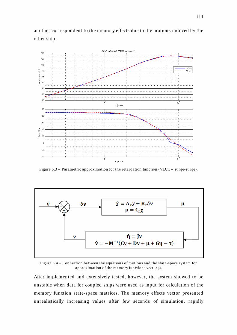
114

another correspondent to the memory effects due to the motions induced by the

other ship.

Figure 6.3 – Parametric approximation for the retardation function (VLCC – surge-surge).

Figure 6.4 – Connection between the equations of motions and the state-space system for

approximation of the memory functions vector 𝛍.

After implemented and extensively tested, however, the system showed to be

unstable when data for coupled ships were used as input for calculation of the

memory function state-space matrices. The memory effects vector presented

unrealistically increasing values after few seconds of simulation, rapidly

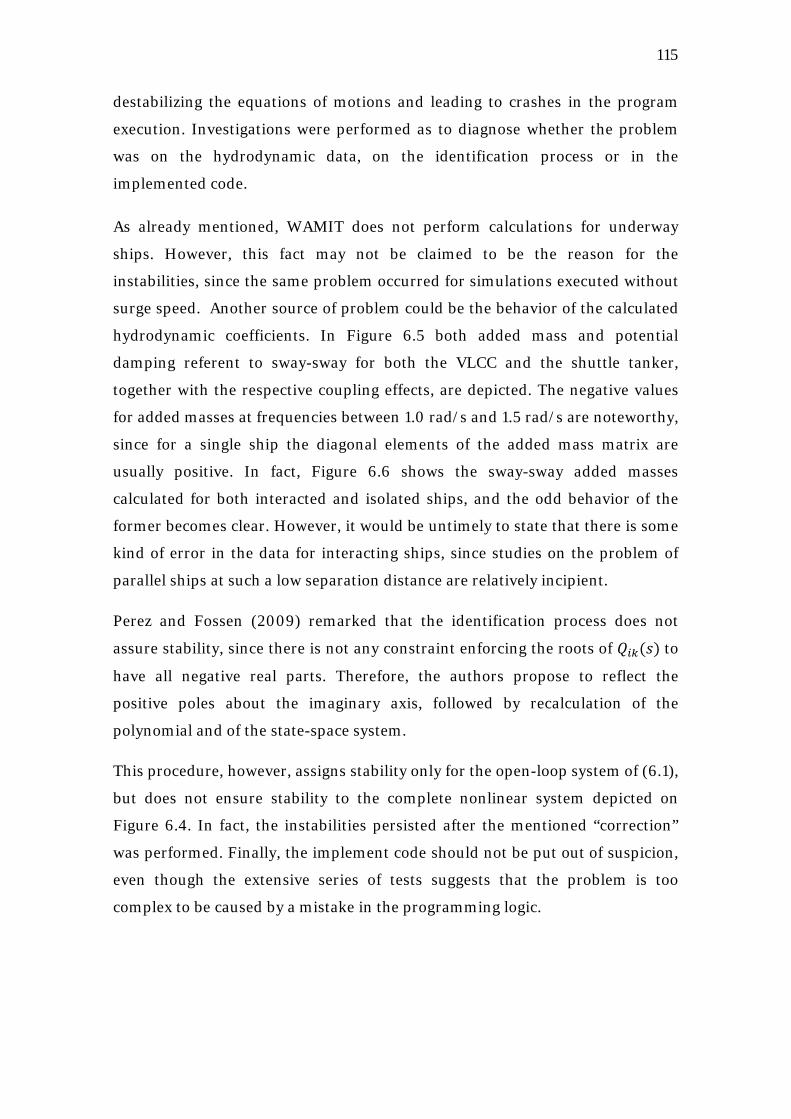
115

destabilizing the equations of motions and leading to crashes in the program

execution. Investigations were performed as to diagnose whether the problem

was on the hydrodynamic data, on the identification process or in the

implemented code.

As already mentioned, WAMIT does not perform calculations for underway

ships. However, this fact may not be claimed to be the reason for the

instabilities, since the same problem occurred for simulations executed without

surge speed. Another source of problem could be the behavior of the calculated

hydrodynamic coefficients. In Figure 6.5 both added mass and potential

damping referent to sway-sway for both the VLCC and the shuttle tanker,

together with the respective coupling effects, are depicted. The negative values

for added masses at frequencies between 1.0 rad/s and 1.5 rad/s are noteworthy,

since for a single ship the diagonal elements of the added mass matrix are

usually positive. In fact, Figure 6.6 shows the sway-sway added masses

calculated for both interacted and isolated ships, and the odd behavior of the

former becomes clear. However, it would be untimely to state that there is some

kind of error in the data for interacting ships, since studies on the problem of

parallel ships at such a low separation distance are relatively incipient.

Perez and Fossen (2009) remarked that the identification process does not

assure stability, since there is not any constraint enforcing the roots of 𝑄𝑖𝑘(𝑠) to

have all negative real parts. Therefore, the authors propose to reflect the

positive poles about the imaginary axis, followed by recalculation of the

polynomial and of the state-space system.

This procedure, however, assigns stability only for the open-loop system of (6.1),

but does not ensure stability to the complete nonlinear system depicted on

Figure 6.4. In fact, the instabilities persisted after the mentioned “correction”

was performed. Finally, the implement code should not be put out of suspicion,

even though the extensive series of tests suggests that the problem is too

complex to be caused by a mistake in the programming logic.

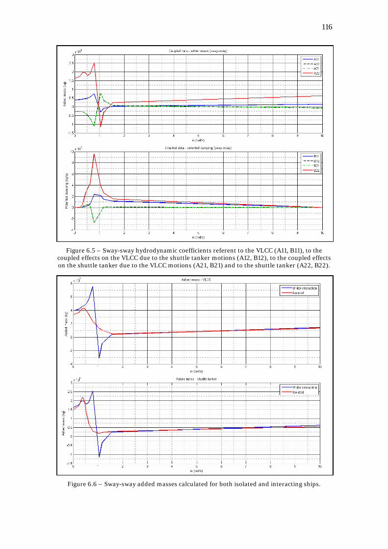
116

Figure 6.5 – Sway-sway hydrodynamic coefficients referent to the VLCC (A11, B11), to the

coupled effects on the VLCC due to the shuttle tanker motions (A12, B12), to the coupled effects on the shuttle tanker due to the VLCC motions (A21, B21) and to the shuttle tanker (A22, B22).

Figure 6.6 – Sway-sway added masses calculated for both isolated and interacting ships.

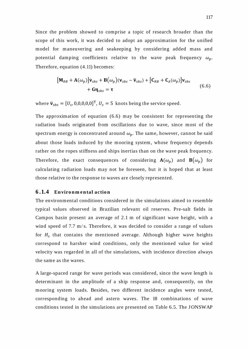
117

Since the problem showed to comprise a topic of research broader than the

scope of this work, it was decided to adopt an approximation for the unified

model for maneuvering and seakeeping by considering added mass and

potential damping coefficients relative to the wave peak frequency 𝜔𝑝.

Therefore, equation (4.11) becomes:

�𝐌𝑅𝐵 + 𝐀(𝜔𝑝)��̇�𝑠𝑏𝑠 + 𝐁�𝜔𝑝�(𝛎𝑠𝑏𝑠 − 𝛎�𝑠𝑏𝑠) + �𝐂𝑅𝐵 + 𝐂𝐴(𝜔𝑝)�𝛎𝑠𝑏𝑠

+ 𝐆𝛈𝑠𝑏𝑠 = 𝛕 (6.6)

where 𝛎�𝑠𝑏𝑠 = [𝑈𝑠, 0,0,0,0,0]T, 𝑈𝑠 = 5 knots being the service speed.

The approximation of equation (6.6) may be consistent for representing the

radiation loads originated from oscillations due to wave, since most of the

spectrum energy is concentrated around 𝜔𝑝. The same, however, cannot be said

about those loads induced by the mooring system, whose frequency depends

rather on the ropes stiffness and ships inertias than on the wave peak frequency.

Therefore, the exact consequences of considering 𝐀(𝜔𝑝) and 𝐁�𝜔𝑝� for

calculating radiation loads may not be foreseen, but it is hoped that at least

those relative to the response to waves are closely represented.

6.1.4 Environmental action The environmental conditions considered in the simulations aimed to resemble

typical values observed in Brazilian relevant oil reserves. Pre-salt fields in

Campos basin present an average of 2.1 m of significant wave height, with a

wind speed of 7.7 m/s. Therefore, it was decided to consider a range of values

for 𝐻𝑠 that contains the mentioned average. Although higher wave heights

correspond to harsher wind conditions, only the mentioned value for wind

velocity was regarded in all of the simulations, with incidence direction always

the same as the waves.

A large-spaced range for wave periods was considered, since the wave length is

determinant in the amplitude of a ship response and, consequently, on the

mooring system loads. Besides, two different incidence angles were tested,

corresponding to ahead and astern waves. The 18 combinations of wave

conditions tested in the simulations are presented on Table 6.5. The JONSWAP

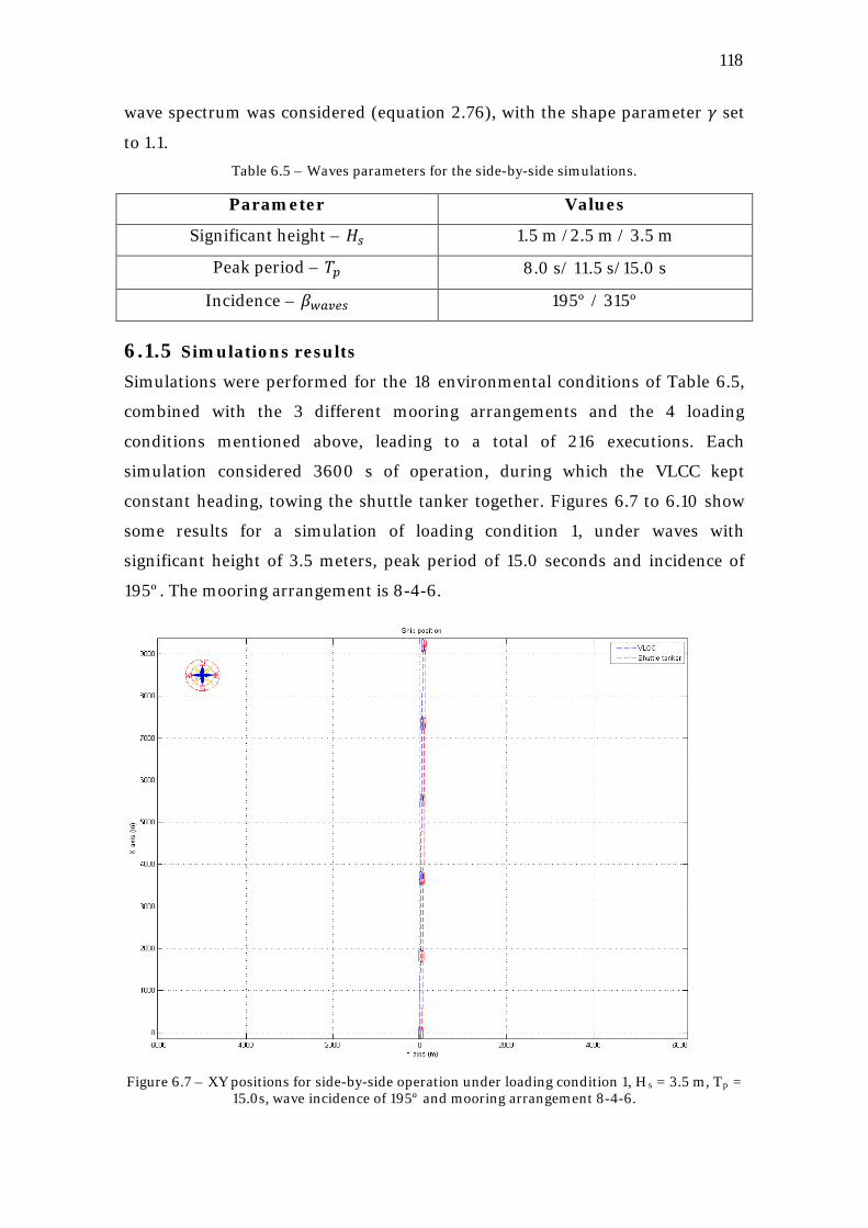
118

wave spectrum was considered (equation 2.76), with the shape parameter 𝛾 set

to 1.1. Table 6.5 – Waves parameters for the side-by-side simulations.

Parameter Values

Significant height – 𝐻𝑠 1.5 m /2.5 m / 3.5 m

Peak period – 𝑇𝑝 8.0 s/ 11.5 s/15.0 s

Incidence – 𝛽𝑤𝑎𝑣𝑒𝑠 195º / 315º

6.1.5 Simulations results Simulations were performed for the 18 environmental conditions of Table 6.5,

combined with the 3 different mooring arrangements and the 4 loading

conditions mentioned above, leading to a total of 216 executions. Each

simulation considered 3600 s of operation, during which the VLCC kept

constant heading, towing the shuttle tanker together. Figures 6.7 to 6.10 show

some results for a simulation of loading condition 1, under waves with

significant height of 3.5 meters, peak period of 15.0 seconds and incidence of

195º. The mooring arrangement is 8-4-6.

Figure 6.7 – XY positions for side-by-side operation under loading condition 1, Hs = 3.5 m, Tp =

15.0s, wave incidence of 195º and mooring arrangement 8-4-6.

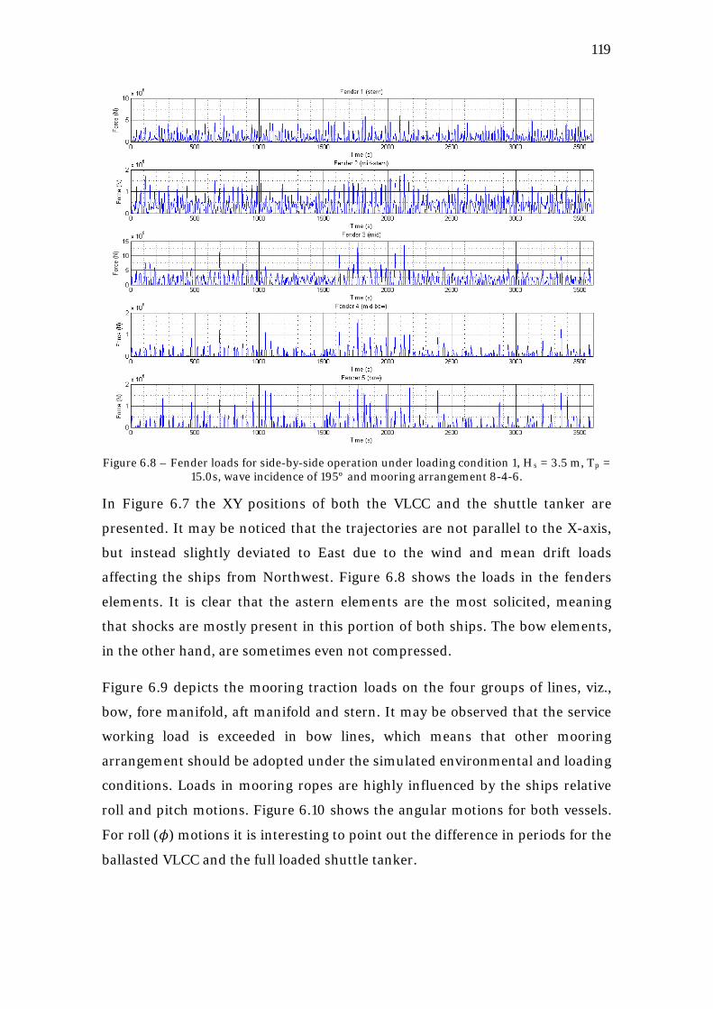
119

Figure 6.8 – Fender loads for side-by-side operation under loading condition 1, Hs = 3.5 m, Tp

In

= 15.0s, wave incidence of 195º and mooring arrangement 8-4-6.

Figure 6.7 the XY positions of both the VLCC and the shuttle tanker are

presented. It may be noticed that the trajectories are not parallel to the X-axis,

but instead slightly deviated to East due to the wind and mean drift loads

affecting the ships from Northwest. Figure 6.8 shows the loads in the fenders

elements. It is clear that the astern elements are the most solicited, meaning

that shocks are mostly present in this portion of both ships. The bow elements,

in the other hand, are sometimes even not compressed.

Figure 6.9 depicts the mooring traction loads on the four groups of lines, viz.,

bow, fore manifold, aft manifold and stern. It may be observed that the service

working load is exceeded in bow lines, which means that other mooring

arrangement should be adopted under the simulated environmental and loading

conditions. Loads in mooring ropes are highly influenced by the ships relative

roll and pitch motions. Figure 6.10 shows the angular motions for both vessels.

For roll (𝜙) motions it is interesting to point out the difference in periods for the

ballasted VLCC and the full loaded shuttle tanker.

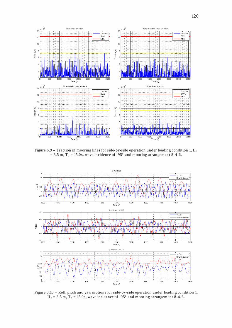
120

Figure 6.9 – Traction in mooring lines for side-by-side operation under loading condition 1, Hs = 3.5 m, Tp

= 15.0s, wave incidence of 195º and mooring arrangement 8-4-6.

Figure 6.10 – Roll, pitch and yaw motions for side-by-side operation under loading condition 1, Hs = 3.5 m, Tp = 15.0s, wave incidence of 195º and mooring arrangement 8-4-6.

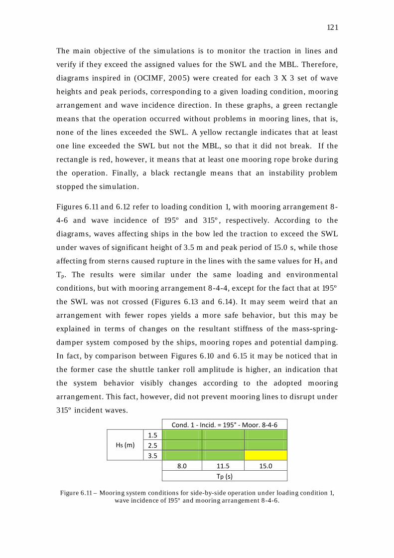
121

The main objective of the simulations is to monitor the traction in lines and

verify if they exceed the assigned values for the SWL and the MBL. Therefore,

diagrams inspired in (OCIMF, 2005) were created for each 3 X 3 set of wave

heights and peak periods, corresponding to a given loading condition, mooring

arrangement and wave incidence direction. In these graphs, a green rectangle

means that the operation occurred without problems in mooring lines, that is,

none of the lines exceeded the SWL. A yellow rectangle indicates that at least

one line exceeded the SWL but not the MBL, so that it did not break. If the

rectangle is red, however, it means that at least one mooring rope broke during

the operation. Finally, a black rectangle means that an instability problem

stopped the simulation.

Figures 6.11 and 6.12 refer to loading condition 1, with mooring arrangement 8-

4-6 and wave incidence of 195º and 315º, respectively. According to the

diagrams, waves affecting ships in the bow led the traction to exceed the SWL

under waves of significant height of 3.5 m and peak period of 15.0 s, while those

affecting from sterns caused rupture in the lines with the same values for Hs and

Tp. The results were similar under the same loading and environmental

conditions, but with mooring arrangement 8-4-4, except for the fact that at 195º

the SWL was not crossed (Figures 6.13 and 6.14). It may seem weird that an

arrangement with fewer ropes yields a more safe behavior, but this may be

explained in terms of changes on the resultant stiffness of the mass-spring-

damper system composed by the ships, mooring ropes and potential damping.

In fact, by comparison between Figures 6.10 and 6.15 it may be noticed that in

the former case the shuttle tanker roll amplitude is higher, an indication that

the system behavior visibly changes according to the adopted mooring

arrangement. This fact, however, did not prevent mooring lines to disrupt under

315º incident waves.

Cond. 1 - Incid. = 195° - Moor. 8-4-6

Hs (m) 1.5 1 1 1 2.5 1 1 1 3.5 1 1 2

8.0 11.5 15.0 Tp (s)

Figure 6.11 – Mooring system conditions for side-by-side operation under loading condition 1, wave incidence of 195º and mooring arrangement 8-4-6.

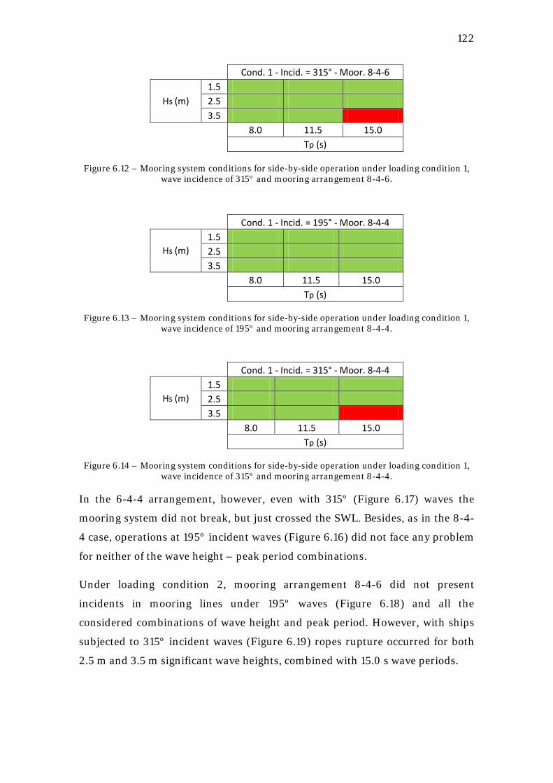
122

Cond. 1 - Incid. = 315° - Moor. 8-4-6

Hs (m) 1.5 1 1 1 2.5 1 1 1 3.5 1 1 3

8.0 11.5 15.0

Tp (s)


Cond. 1 - Incid. = 195° - Moor. 8-4-4

Hs (m) 1.5 1 1 1 2.5 1 1 1 3.5 1 1 1

8.0 11.5 15.0

Tp (s)


Cond. 1 - Incid. = 315° - Moor. 8-4-4

Hs (m) 1.5 1 1 1 2.5 1 1 1 3.5 1 1 3

8.0 11.5 15.0

Tp (s)


In the 6-4-4 arrangement, however, even with 315º (Figure 6.17) waves the

mooring system did not break, but just crossed the SWL. Besides, as in the 8-4-

4 case, operations at 195º incident waves (Figure 6.16) did not face any problem

for neither of the wave height – peak period combinations.

Under loading condition 2, mooring arrangement 8-4-6 did not present

incidents in mooring lines under 195º waves (Figure 6.18) and all the

considered combinations of wave height and peak period. However, with ships

subjected to 315º incident waves (Figure 6.19) ropes rupture occurred for both

2.5 m and 3.5 m significant wave heights, combined with 15.0 s wave periods.

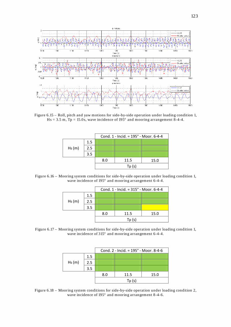
123

Figure 6.15 – Roll, pitch and yaw motions for side-by-side operation under loading condition 1,

Hs = 3.5 m, Tp = 15.0s, wave incidence of 195º and mooring arrangement 8-4-4.

Cond. 1 - Incid. = 195° - Moor. 6-4-4

Hs (m) 1.5 1 1 1 2.5 1 1 1 3.5 1 1 1

8.0 11.5 15.0

Tp (s)


Cond. 1 - Incid. = 315° - Moor. 6-4-4

Hs (m) 1.5 1 1 1 2.5 1 1 1 3.5 1 1 2

8.0 11.5 15.0

Tp (s)


Cond. 2 - Incid. = 195° - Moor. 8-4-6

Hs (m) 1.5 1 1 1 2.5 1 1 1 3.5 1 1 1

8.0 11.5 15.0

Tp (s)


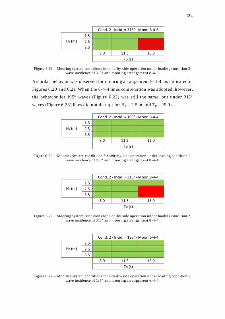
124

Cond. 2 - Incid. = 315° - Moor. 8-4-6

Hs (m) 1.5 1 1 1 2.5 1 1 3 3.5 1 1 3

8.0 11.5 15.0

Tp (s)


A similar behavior was observed for mooring arrangement 8-4-4, as indicated in

Figures 6.20 and 6.21. When the 6-4-4 lines combination was adopted, however,

the behavior for 195º waves (Figure 6.22) was still the same, but under 315º

waves (Figure 6.23) lines did not disrupt for Hs = 2.5 m and Tp = 15.0 s.

Cond. 2 - Incid. = 195° - Moor. 8-4-4

Hs (m) 1.5 1 1 1 2.5 1 1 1 3.5 1 1 1

8.0 11.5 15.0

Tp (s)


Cond. 2 - Incid. = 315° - Moor. 8-4-4

Hs (m) 1.5 1 1 1 2.5 1 1 3 3.5 1 1 3

8.0 11.5 15.0

Tp (s)


Cond. 2 - Incid. = 195° - Moor. 6-4-4

Hs (m) 1.5 1 1 1 2.5 1 1 1 3.5 1 1 1

8.0 11.5 15.0

Tp (s)


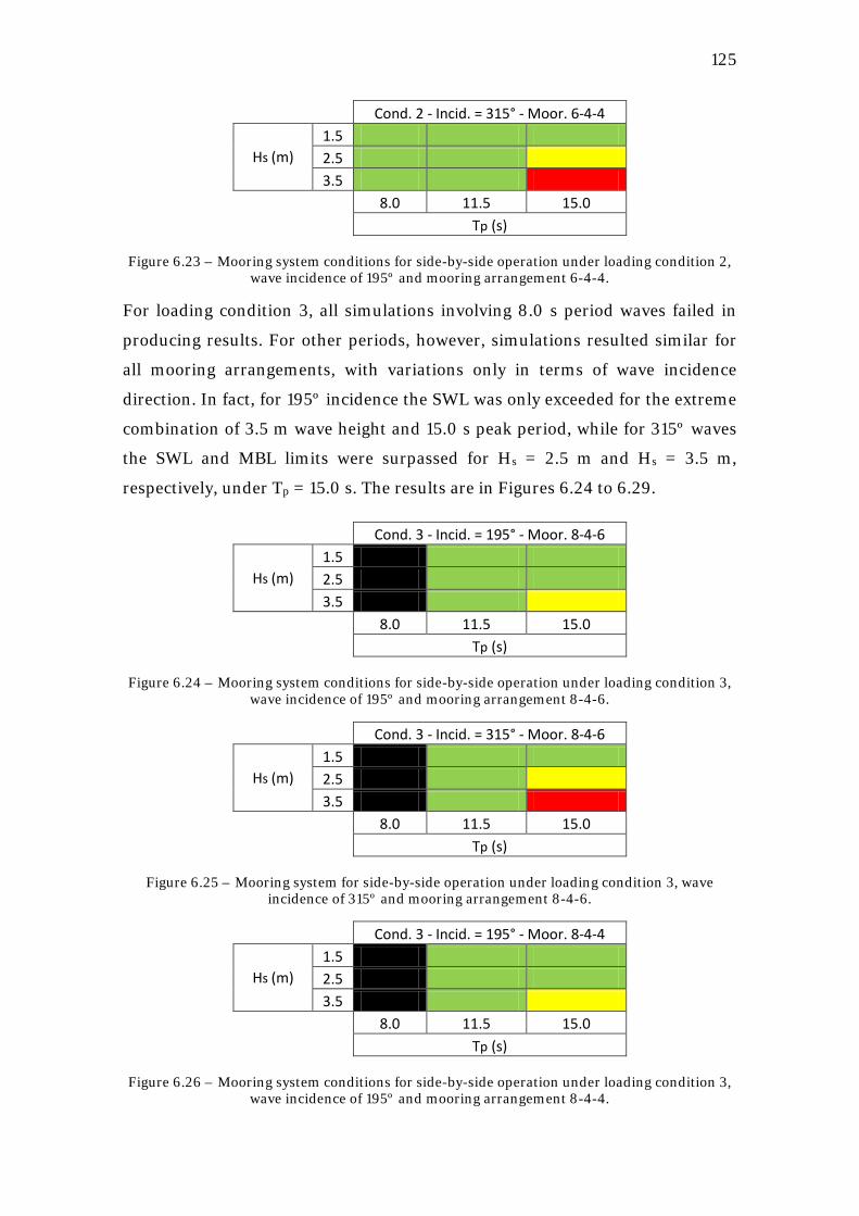
125

Cond. 2 - Incid. = 315° - Moor. 6-4-4

Hs (m) 1.5 1 1 1 2.5 1 1 2 3.5 1 1 3

8.0 11.5 15.0

Tp (s)


For loading condition 3, all simulations involving 8.0 s period waves failed in

producing results. For other periods, however, simulations resulted similar for

all mooring arrangements, with variations only in terms of wave incidence

direction. In fact, for 195º incidence the SWL was only exceeded for the extreme

combination of 3.5 m wave height and 15.0 s peak period, while for 315º waves

the SWL and MBL limits were surpassed for Hs = 2.5 m and Hs = 3.5 m,

respectively, under Tp = 15.0 s. The results are in Figures 6.24 to 6.29.

Cond. 3 - Incid. = 195° - Moor. 8-4-6

Hs (m) 1.5 4 1 1 2.5 4 1 1 3.5 4 1 2

8.0 11.5 15.0

Tp (s)


Cond. 3 - Incid. = 315° - Moor. 8-4-6

Hs (m) 1.5 4 1 1 2.5 4 1 2 3.5 4 1 3

8.0 11.5 15.0

Tp (s)

Figure 6.25 – Mooring system for side-by-side operation under loading condition 3, wave incidence of 315º and mooring arrangement 8-4-6.

Cond. 3 - Incid. = 195° - Moor. 8-4-4

Hs (m) 1.5 4 1 1 2.5 4 1 1 3.5 4 1 2

8.0 11.5 15.0

Tp (s)


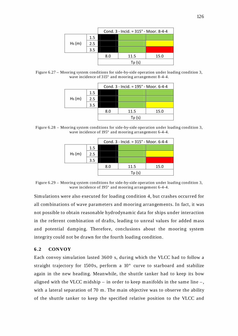
126

Cond. 3 - Incid. = 315° - Moor. 8-4-4

Hs (m) 1.5 4 1 1 2.5 4 1 2 3.5 4 1 3

8.0 11.5 15.0

Tp (s)


Cond. 3 - Incid. = 195° - Moor. 6-4-4

Hs (m) 1.5 4 1 1 2.5 4 1 1 3.5 4 1 2

8.0 11.5 15.0

Tp (s)


Cond. 3 - Incid. = 315° - Moor. 6-4-4

Hs (m) 1.5 4 1 1 2.5 4 1 2 3.5 4 1 3

8.0 11.5 15.0

Tp (s)


Simulations were also executed for loading condition 4, but crashes occurred for

all combinations of wave parameters and mooring arrangements. In fact, it was

not possible to obtain reasonable hydrodynamic data for ships under interaction

in the referent combination of drafts, leading to unreal values for added mass

and potential damping. Therefore, conclusions about the mooring system

integrity could not be drawn for the fourth loading condition.

6.2 CONVOY

Each convoy simulation lasted 3600 s, during which the VLCC had to follow a

straight trajectory for 1500s, perform a 10º curve to starboard and stabilize

again in the new heading. Meanwhile, the shuttle tanker had to keep its bow

aligned with the VLCC midship – in order to keep manifolds in the same line –,

with a lateral separation of 70 m. The main objective was to observe the ability

of the shuttle tanker to keep the specified relative position to the VLCC and

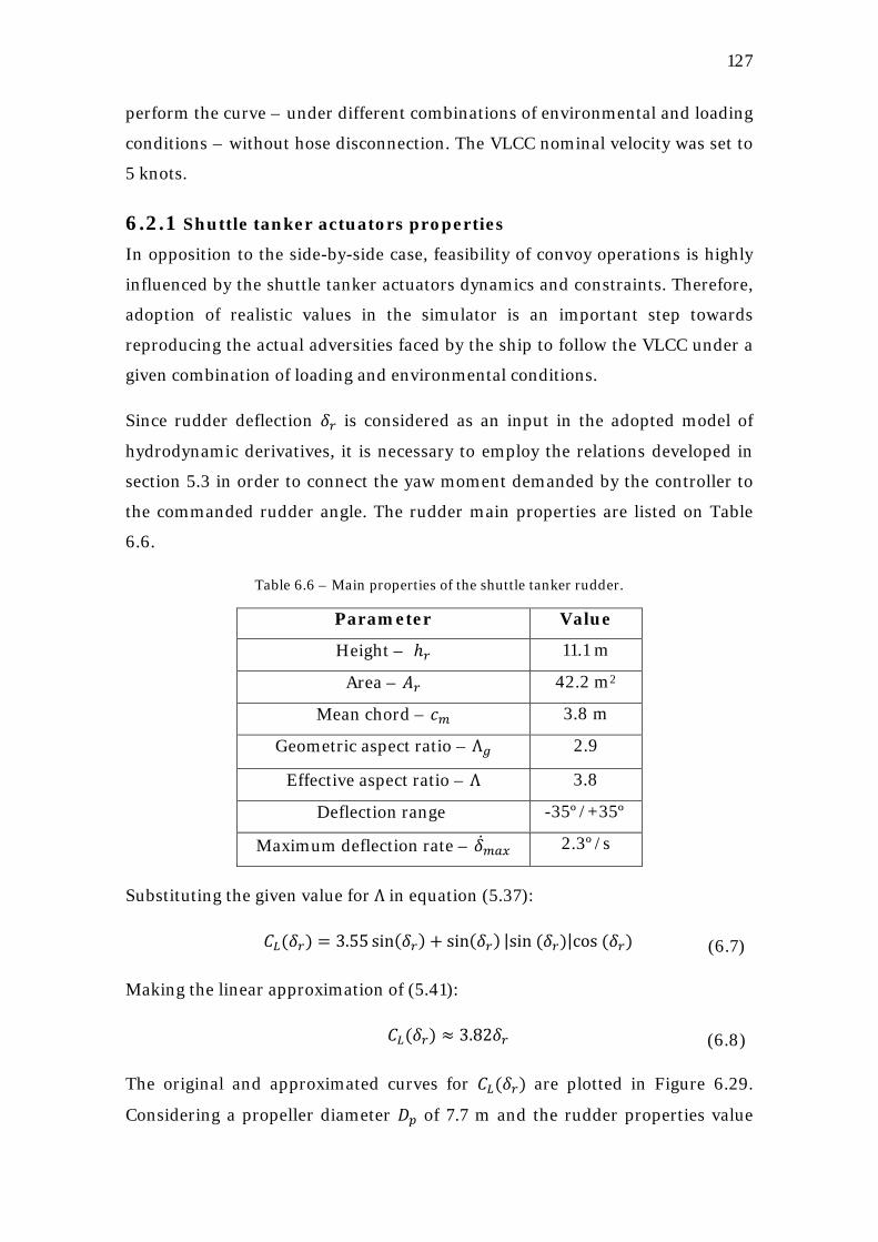
127

perform the curve – under different combinations of environmental and loading

conditions – without hose disconnection. The VLCC nominal velocity was set to

5 knots.

6.2.1 Shuttle tanker actuators properties In opposition to the side-by-side case, feasibility of convoy operations is highly

influenced by the shuttle tanker actuators dynamics and constraints. Therefore,

adoption of realistic values in the simulator is an important step towards

reproducing the actual adversities faced by the ship to follow the VLCC under a

given combination of loading and environmental conditions.

Since rudder deflection 𝛿𝑟 is considered as an input in the adopted model of

hydrodynamic derivatives, it is necessary to employ the relations developed in

section 5.3 in order to connect the yaw moment demanded by the controller to

the commanded rudder angle. The rudder main properties are listed on Table

6.6.

Table 6.6 – Main properties of the shuttle tanker rudder.

Parameter Value

Height – ℎ𝑟 11.1 m

Area – 𝐴𝑟 42.2 m2

Mean chord – 𝑐𝑚 3.8 m

Geometric aspect ratio – Λ𝑔 2.9

Effective aspect ratio – Λ 3.8

Deflection range -35º/+35º

Maximum deflection rate – �̇�𝑚𝑎𝑥 2.3º/s

Substituting the given value for Λ in equation (5.37):

𝐶𝐿(𝛿𝑟) = 3.55 sin(𝛿𝑟) + sin(𝛿𝑟) |sin (𝛿𝑟)|cos (𝛿𝑟) (6.7)

Making the linear approximation of (5.41):

𝐶𝐿(𝛿𝑟) ≈ 3.82𝛿𝑟 (6.8)

The original and approximated curves for 𝐶𝐿(𝛿𝑟) are plotted in Figure 6.29.

Considering a propeller diameter 𝐷𝑝 of 7.7 m and the rudder properties value

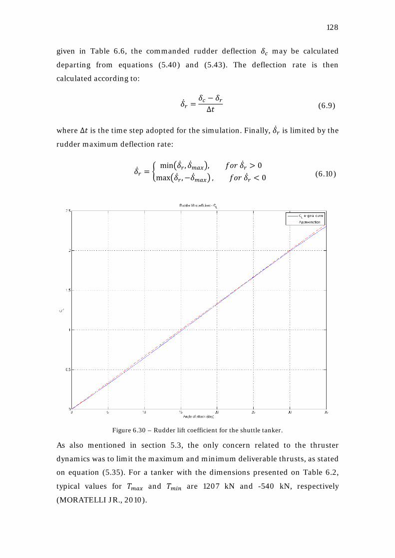
128

given in Table 6.6, the commanded rudder deflection 𝛿𝑐 may be calculated

departing from equations (5.40) and (5.43). The deflection rate is then

calculated according to:

�̇�𝑟 =𝛿𝑐 − 𝛿𝑟Δ𝑡

(6.9)

where Δ𝑡 is the time step adopted for the simulation. Finally, �̇�𝑟 is limited by the

rudder maximum deflection rate:

�̇�𝑟 = �min��̇�𝑟 , �̇�𝑚𝑎𝑥�, 𝑓𝑜𝑟 �̇�𝑟 > 0

max��̇�𝑟 ,−�̇�𝑚𝑎𝑥� , 𝑓𝑜𝑟 �̇�𝑟 < 0� (6.10)

Figure 6.30 – Rudder lift coefficient for the shuttle tanker.

As also mentioned in section 5.3, the only concern related to the thruster

dynamics was to limit the maximum and minimum deliverable thrusts, as stated

on equation (5.35). For a tanker with the dimensions presented on Table 6.2,

typical values for 𝑇𝑚𝑎𝑥 and 𝑇𝑚𝑖𝑛 are 1207 kN and -540 kN, respectively

(MORATELLI JR., 2010).

129

6.2.2 Environmental action The environmental conditions considered for the side-by-side simulations are

not necessarily the most relevant for the convoy operations. While in the former

case wave length has a critical connection to the mooring system response, in

the latter the concern is mostly directed for loads that may hamper the shuttle

tanker ability to follow the VLCC. In this sense, stern waves were not

considered, while the ships responses to a larger incidence angle were tested.

The wave parameters of Table 6.7 were adopted for the convoy operation

simulations. Wave motions were considered by superposition of low- and wave-

frequency motions, according to the procedure on Figure 2.9. Wind velocity was

set to 7.7 m/s and the direction was always coincident to waves, but simulations

without wind were also executed in order to evaluate the influence of this load

on the shuttle tanker controllability for the different ships loading conditions.

As in the side-by-side case, it was decided not to consider ocean current in the

simulations.

Table 6.7 – Waves parameters for the convoy simulations.

Parameter Values

Significant height – 𝐻𝑠 1.5 m / 3.5 m

Peak period – 𝑇𝑝 8.0 s/ 11.5 s

Incidence – 𝛽𝑤𝑎𝑣𝑒𝑠 120º / 195º

6.2.3 Simulations results All combinations of environmental and loading conditions were simulated,

leading to a total of 48 executions. The criteria established to evaluate the

operation safety under a given condition were hose disconnection – that may be

caused if the shuttle tanker loses its ability to follow the VLCC – and risk of

collision.

Figure 6.31 illustrates the definitions of the distance between manifolds 𝐷𝑚𝑓 and

of the separation distance 𝑦𝑠𝑒𝑝. For a given hose length 𝑙ℎ, it was considered that

a disconnection occurred if 𝐷𝑚𝑓 > 𝑙ℎ for any instant of the operation. Besides, a

collision was detected always that 𝑦𝑠𝑒𝑝 ≤ 𝑦𝑚𝑖𝑛 was verified, for a given value of

the minimum safe distance 𝑦𝑚𝑖𝑛.

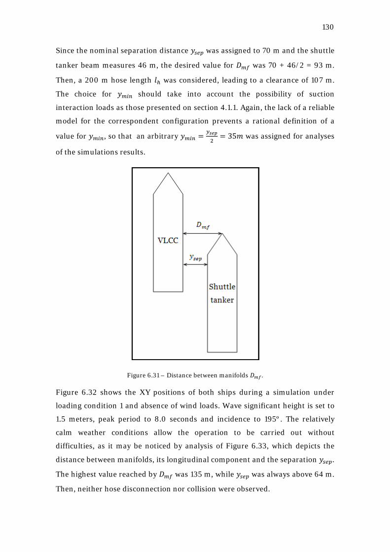
130

Since the nominal separation distance 𝑦𝑠𝑒𝑝 was assigned to 70 m and the shuttle

tanker beam measures 46 m, the desired value for 𝐷𝑚𝑓 was 70 + 46/2 = 93 m.

Then, a 200 m hose length 𝑙ℎ was considered, leading to a clearance of 107 m.

The choice for 𝑦𝑚𝑖𝑛 should take into account the possibility of suction

interaction loads as those presented on section 4.1.1. Again, the lack of a reliable

model for the correspondent configuration prevents a rational definition of a

value for 𝑦𝑚𝑖𝑛, so that an arbitrary 𝑦𝑚𝑖𝑛 = 𝑦𝑠𝑒𝑝2

= 35𝑚 was assigned for analyses

of the simulations results.

Figure 6.31 – Distance between manifolds 𝐷𝑚𝑓.

Figure 6.32 shows the XY positions of both ships during a simulation under

loading condition 1 and absence of wind loads. Wave significant height is set to

1.5 meters, peak period to 8.0 seconds and incidence to 195º. The relatively

calm weather conditions allow the operation to be carried out without

difficulties, as it may be noticed by analysis of Figure 6.33, which depicts the

distance between manifolds, its longitudinal component and the separation 𝑦𝑠𝑒𝑝.

The highest value reached by 𝐷𝑚𝑓 was 135 m, while 𝑦𝑠𝑒𝑝 was always above 64 m.

Then, neither hose disconnection nor collision were observed.

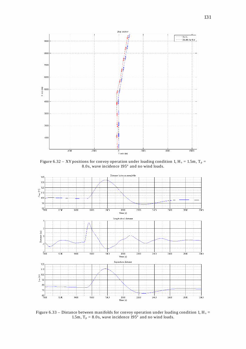
131

Figure 6.32 – XY positions for convoy operation under loading condition 1, Hs = 1.5m, Tp

= 8.0s, wave incidence 195º and no wind loads.

Figure 6.33 – Distance between manifolds for convoy operation under loading condition 1, Hs = 1.5m, Tp = 8.0s, wave incidence 195º and no wind loads.

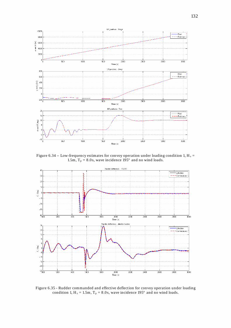
132

Figure 6.34 – Low-frequency estimates for convoy operation under loading condition 1, Hs = 1.5m, Tp

= 8.0s, wave incidence 195º and no wind loads.

Figure 6.35 - Rudder commanded and effective deflection for convoy operation under loading condition 1, Hs = 1.5m, Tp = 8.0s, wave incidence 195º and no wind loads.

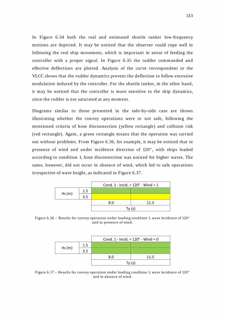
133

In Figure 6.34 both the real and estimated shuttle tanker low-frequency

motions are depicted. It may be noticed that the observer could cope well in

following the real ship movement, which is important in sense of feeding the

controller with a proper signal. In Figure 6.35 the rudder commanded and

effective deflections are plotted. Analysis of the curve correspondent to the

VLCC shows that the rudder dynamics prevent the deflection to follow excessive

modulation induced by the controller. For the shuttle tanker, in the other hand,

it may be noticed that the controller is more sensitive to the ship dynamics,

since the rudder is not saturated at any moment.

Diagrams similar to those presented in the side-by-side case are shown

illustrating whether the convoy operations were or not safe, following the

mentioned criteria of hose disconnection (yellow rectangle) and collision risk

(red rectangle). Again, a green rectangle means that the operation was carried

out without problems. From Figure 6.36, for example, it may be noticed that in

presence of wind and under incidence direction of 120º, with ships loaded

according to condition 1, hose disconnection was noticed for higher waves. The

same, however, did not occur in absence of wind, which led to safe operations

irrespective of wave height, as indicated in Figure 6.37.

Cond. 1 - Incid. = 120° - Wind = 1

Hs (m) 1.5 1.00 1.00 3.5 3.00 3.00

8.0 11.5

Tp (s)

Figure 6.36 – Results for convoy operation under loading condition 1, wave incidence of 120º and in presence of wind.

Cond. 1 - Incid. = 120° - Wind = 0

Hs (m) 1.5 1.00 1.00 3.5 1.00 1.00

8.0 11.5

Tp (s)

Figure 6.37 – Results for convoy operation under loading condition 1, wave incidence of 120º and in absence of wind.

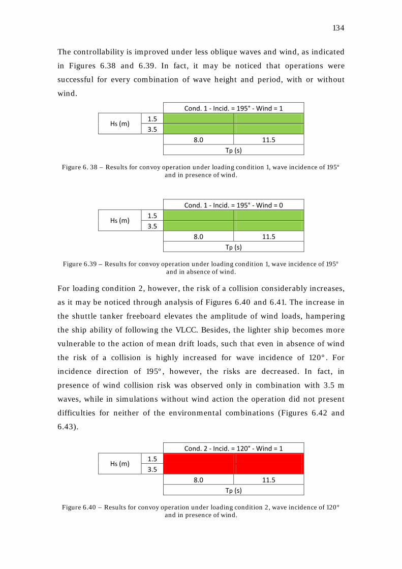
134

The controllability is improved under less oblique waves and wind, as indicated

in Figures 6.38 and 6.39. In fact, it may be noticed that operations were

successful for every combination of wave height and period, with or without

wind. Cond. 1 - Incid. = 195° - Wind = 1

Hs (m) 1.5 1.00 1.00 3.5 1.00 1.00

8.0 11.5

Tp (s)

Figure 6. 38 – Results for convoy operation under loading condition 1, wave incidence of 195º and in presence of wind.

Cond. 1 - Incid. = 195° - Wind = 0

Hs (m) 1.5 1.00 1.00 3.5 1.00 1.00

8.0 11.5

Tp (s)


For loading condition 2, however, the risk of a collision considerably increases,

as it may be noticed through analysis of Figures 6.40 and 6.41. The increase in

the shuttle tanker freeboard elevates the amplitude of wind loads, hampering

the ship ability of following the VLCC. Besides, the lighter ship becomes more

vulnerable to the action of mean drift loads, such that even in absence of wind

the risk of a collision is highly increased for wave incidence of 120º. For

incidence direction of 195º, however, the risks are decreased. In fact, in

presence of wind collision risk was observed only in combination with 3.5 m

waves, while in simulations without wind action the operation did not present

difficulties for neither of the environmental combinations (Figures 6.42 and

6.43).

Cond. 2 - Incid. = 120° - Wind = 1

Hs (m) 1.5 2.00 2.00 3.5 2.00 2.00

8.0 11.5

Tp (s)


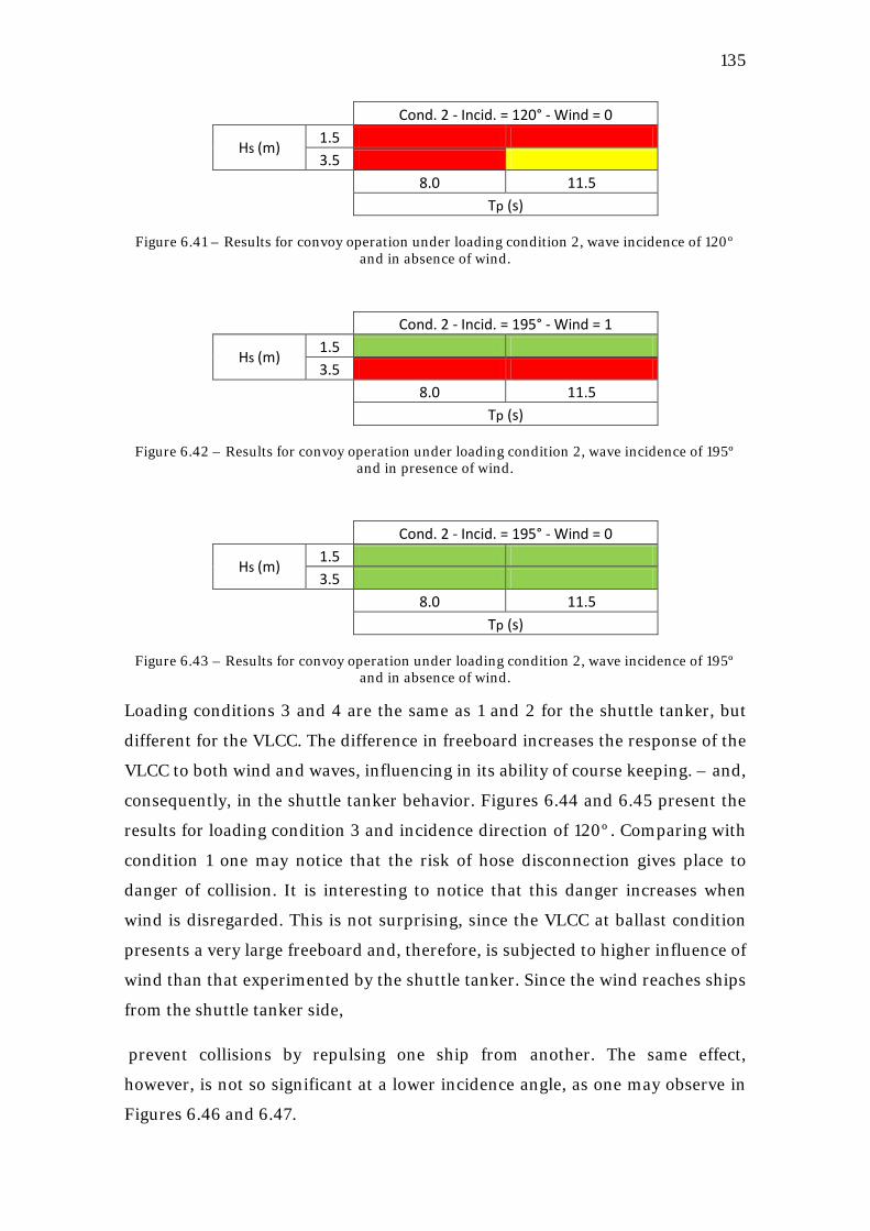
135

Cond. 2 - Incid. = 120° - Wind = 0

Hs (m) 1.5 2.00 2.00 3.5 2.00 3.00

8.0 11.5

Tp (s)


Cond. 2 - Incid. = 195° - Wind = 1

Hs (m) 1.5 1.00 1.00 3.5 2.00 2.00

8.0 11.5

Tp (s)


Cond. 2 - Incid. = 195° - Wind = 0

Hs (m) 1.5 1.00 1.00 3.5 1.00 1.00

8.0 11.5

Tp (s)


Loading conditions 3 and 4 are the same as 1 and 2 for the shuttle tanker, but

different for the VLCC. The difference in freeboard increases the response of the

VLCC to both wind and waves, influencing in its ability of course keeping. – and,

consequently, in the shuttle tanker behavior. Figures 6.44 and 6.45 present the

results for loading condition 3 and incidence direction of 120º. Comparing with

condition 1 one may notice that the risk of hose disconnection gives place to

danger of collision. It is interesting to notice that this danger increases when

wind is disregarded. This is not surprising, since the VLCC at ballast condition

presents a very large freeboard and, therefore, is subjected to higher influence of

wind than that experimented by the shuttle tanker. Since the wind reaches ships

from the shuttle tanker side,

prevent collisions by repulsing one ship from another. The same effect,

however, is not so significant at a lower incidence angle, as one may observe in

Figures 6.46 and 6.47.

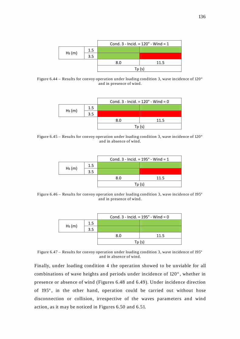
136

Cond. 3 - Incid. = 120° - Wind = 1

Hs (m) 1.5 1.00 1.00 3.5 1.00 2.00

8.0 11.5

Tp (s)


Cond. 3 - Incid. = 120° - Wind = 0

Hs (m) 1.5 1.00 1.00 3.5 2.00 2.00

8.0 11.5

Tp (s)


Cond. 3 - Incid. = 195° - Wind = 1

Hs (m) 1.5 1.00 1.00 3.5 1.00 2.00

8.0 11.5

Tp (s)


Cond. 3 - Incid. = 195° - Wind = 0

Hs (m) 1.5 1.00 1.00 3.5 1.00 1.00

8.0 11.5

Tp (s)


Finally, under loading condition 4 the operation showed to be unviable for all

combinations of wave heights and periods under incidence of 120º, whether in

presence or absence of wind (Figures 6.48 and 6.49). Under incidence direction

of 195º, in the other hand, operation could be carried out without hose

disconnection or collision, irrespective of the waves parameters and wind

action, as it may be noticed in Figures 6.50 and 6.51.

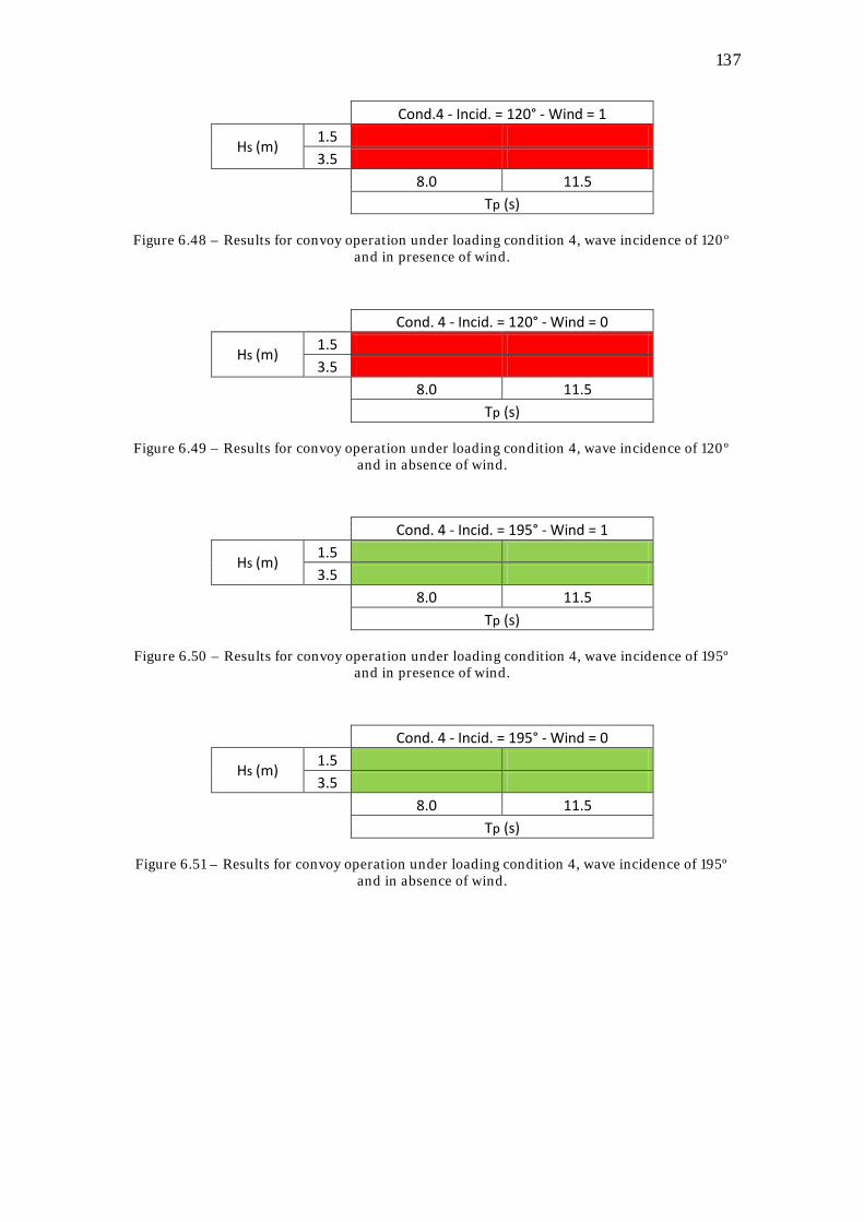
137

Cond.4 - Incid. = 120° - Wind = 1

Hs (m) 1.5 2.00 2.00 3.5 2.00 2.00

8.0 11.5

Tp (s)


Cond. 4 - Incid. = 120° - Wind = 0

Hs (m) 1.5 2.00 2.00 3.5 2.00 2.00

8.0 11.5

Tp (s)


Cond. 4 - Incid. = 195° - Wind = 1

Hs (m) 1.5 1.00 1.00 3.5 1.00 1.00

8.0 11.5

Tp (s)


Cond. 4 - Incid. = 195° - Wind = 0

Hs (m) 1.5 1.00 1.00 3.5 1.00 1.00

8.0 11.5

Tp (s)


138

7. CONCLUSIONS Although both operations have the same goal – transfer of oil between two

underway ships in open sea –, the theoretical aspects behind their models are

considerably different, so that two very distinct problems were approached in

this work. In the side-by-side operation the problem was rather focused on the

dynamics of coupled floating bodies, while in the convoy case attention was

devoted for the development of a refined control approach composed by a

nonlinear set of controller and observer, together with a guidance system.

7.1 SIDE-BY-SIDE

The problem of underway coupled ships subjected to waves demands

application of the unified model for maneuvering and seakeeping presented on

section (2.7.3), which is based on convolution integrals of retardation functions

– representing the fluid memory effects – in order to make possible the

consideration of non-zero frequency loads in the equations of motions. In this

sense, one of the contributions of this work is the application of this approach to

the modeling of underway side-by-side operations, together with models for

other relevant loads like those induced by fenders and mooring system.

It was frustrating that stability problems faced during the simulations prevented

the achievement of outcomes correspondent to the derived model, so that the

results presented on Chapter 6 are actually based on an approximation of this

model. However, the process of understanding the necessary theoretical

background and applying it in a practical problem were indeed the highest

profit along the development of this work.

In fact, the notion of considering fluid memory effects in the equations of

motions for a floating body is extensible for a broad range of practical

applications where two or more bodies share common loads. Besides, it

provides a rather physical comprehension of the response of a ship to waves

than the traditional practice of superposing low- and wave-frequency motions

derived from separate models. The difference becomes clear if one considers, for

example, a ship oscillating in pitch. If the ship is asymmetric in the yz-plane, the

waves radiated by the bow are different from those produced by the stern

motions, so that the resultant in the x direction is not zero, leading to a

139

displacement in surge. This effect is not preserved by the superposition method,

since the radiation loads for non-zero frequency motions are not considered in

the body dynamics.

Analysis of the side-by-side simulations outputs allows some general

conclusions to be drawn. Firstly, irrespective of the loading case the values for

the SWL and the MBL assigned for mooring lines were only exceeded for the

15.0s peak period waves. This means that longer waves have more influence on

ships motions and, consequently, on the mooring system loads. Wave incidence

direction also showed to be determinant for the integrity of the mooring ropes.

The effects presented to be more intense for waves reaching the ships from stern

than those from bow.

An interesting conclusion relates to the different mooring arrangements tested

in the simulations. In spite of presenting a lower number of lines, the 6-4-4

arrangement showed to be safer than the 8-4-6 and 8-4-4 arrangements. This

may be explained in terms of the resultant stiffness of the mooring system,

which has influence on the natural frequency of oscillation of the coupled ships.

7.2 CONVOY

Modeling of convoy operation was based on a less sophisticated approach for

expressing the ships dynamics. The autopilot, however, was based on modern

nonlinear solutions for the observer and controller, together with a guidance

system particularly designed for the task.

The line-of-sight approach was adopted for generation of heading references for

the controller, while a strategy for waypoints generation was developed as to

make the shuttle tanker to keep a given distance to the VLCC. The surge velocity

reference was determined with basis on comparison between the actual and

desired longitudinal distances, resembling solutions of cooperative control. The

resultant guidance system could be adapted for a more ample class of problems

involving control of unmanned vehicles.

Simulations showed a strong dependence of the loading conditions on the

occurrence of hose disconnections and risk of collisions. The freeboard highly

influenced the controllability of the shuttle tanker, mainly under action of

oblique waves and, mostly important, wind. In fact, the ship under ballast

140

condition presents a higher area above water level, so that wind loads become

more pronounced. Besides, the lower ship displacement makes the vessel more

susceptible to the action of both wave mean drift and wind loads, increasing the

necessary control loads to properly follow the VLCC.

In this sense, it was observed that under loading conditions 2 and 4 – those

correspondent to the ballasted shuttle tanker – the operation became unviable

for 120º waves and wind. Since these conditions refer to the end of those

operations initiated at conditions 1 and 3, respectively, the conclusion is that the

whole transfer processes are unpractical for the mentioned angle of incidence.

By diminishing the incidence direction, however, the risk of disconnections and

collisions significantly decreases. In this case, lack of safety was only observed

for condition 2 under 3.5 m significant height waves, irrespective of the peak

period.

7.3 FINAL CONSIDERATIONS AND RECOMMENDATIONS FOR

FUTURE WORK

As already mentioned, this work approached two problems linked by a common

final objective, but of very distinct nature in theoretical terms. It is true that it

could be more fruitful to focus in one of the operations and develop a deeper

and more specific study on its peculiarities. However, the decision to deepen in

different issues becomes more understandable if one considers that the primary

aim of the research was to propose models for two alternatives for oil transfer

between underway tankers.

Also, by introducing a wide range of topics this work proposes a variety of

further research themes. Certainly, investigations on the instabilities verified on

the side-by-side case would yield helpful advances on the matter of using the

state-space approximation of the convolution terms in the equations of motions.

Besides, a theoretical understanding on the wave hydrodynamic interactions is

essential to explain the fluid behavior between hulls, while experiments with

scale models are mandatory for a rational adjustment of the lid method

presented on Chapter 4.

For the convoy case, it would be interesting to test different control strategies

than those approached on this work. Besides, adoption of the so-called high-lift

141

rudders could improve the shuttle tanker maneuvering skills, leading to more

safe operations. Controllability could also be enhanced by usage of the shuttle

tanker azimuthal thruster, if available. Improvement of the proposed guidance

system could also render more satisfactory results than those obtained in this

work. It could be profitable, for example, to determine different criteria for

way-points generation in terms of the environmental conditions. Finally, studies

on the possible suction effects, in the sense of assigning a rational criterion for

collision risk, would aggregate a rather scientific character to the analysis.

142

REFERENCES

ABKOWITZ, M. A. Lectures on ship hydrodyamics - steering and maneuverability. Hydro- and Aerodynamics Laboratory. Lyngby, Denmark, 1964.

ARANHA, J. A. P. Second order horizontal steady forces and moment on a floating body with small forward speed. Journal of Fluid Mechanics, 313, 1996.

ÅSTRÖM, K. J.; HÄGGLUND, T. PID Controllers: Theory, Design, and Tuning. 2. ed. Durham, USA: ISA, 1995.

BAILEY, P. A.; PRICE, W. G.; TEMAREL, P. A unified mathematical model describing the maneuvering of a ship travelling in a seaway. Transactions of the Royal Institution of Naval Architects, 140, pp. 131-139, 1997.

BERG, T. E.; BAKKE, J. Ship-to-ship LNG transfer in arctic waters. Proc. of the ASME 27th International Conference on Offshore Mechanics and Arctic Engineering (OMAE 2008). Estoril, Portugal, 2008.

BERTRAM, V. Practical ship hydrodynamics. Woburn, USA: Butterworth Heinemann, 2000.

BREIVIK, M. Nonlinear maneuvering control of underactuated ships. M.Sc. thesis. Norwegian University of Science and Technology. Trondheim, Norway, 2003.

BREIVIK, M. Topics in guided motion control of marine vehicles. Ph.D. thesis. Norwegian University of Science and Technology. Trondheim, Norway, 2010.

BREIVIK, M.; HOVSTEIN, V. E.; FOSSEN, T. I. Straight-line target tracking for unmaned surface vehicles. Modeling, Identification and Control, 29, n. 4, pp. 131-149, 2008.

BUCHNER, B.; BUNNIK, T. Wind shielding investigations for FPSO tandem offloading. Proc. of The 12th International Offshore and Polar Engineering Conference (ISOPE 2002). Kitakyushu, Japan, 2002.

BUCHNER, B.; VAN DIJK, A.; DE WILDE, J. Numerical multiple-body simulations of side-by-side mooring to an FPSO. Proc. of the 11th International Offshore and Polar Engineering Conference (OMAE 2001). Stavanger, Norway, 2001.

CHEN, G. R.; FANG, M. C. Hydrodynamic interactions between two ships advancing in waves. Ocean Engineering, 28, pp. 1053-1078, 2001.

143

CUMMINS, W. E. The impulse response function and ship motions. David Taylor Model Basin, USA, 1962.

DE DECKER, B. Ship-ship interaction during lightering operations. M.Sc. thesis. Gent University, Gent, Belgium, 2006.

DORF, R. C.; BISHOP, R. H. Modern control systems. New Jersey, USA: Prentice-Hall, 2001.

EVERGREEN. Evergreen-marine fenders, pneumatic fenders, airbags, 2011. Available at: <http://www.qingdaoyongtai.com/en/>. Accessed August 6th, 2011.

FALTINSEN, O. M. Sea loads on ships and offshore structures. Cambridge, UK: Cambridge University Press, 1990.

FORCE TECHNOLOGY. Manoeuvring tests with a model of a 258m Suezmax tanker in loaded condition: DMI 2002189. DMI. Lingby, Denmark, 2002.

FOSSEN, T. I. Nonlinear modeling of and control of underwater vehicles. Ph.D. thesis. Norwegian University of Science and Technology. Trondheim, Norway, 1991.

FOSSEN, T. I. Guidance and control of ocean vehicles. Chichester, England: John Wiley & Sons, 1994.

FOSSEN, T. I. Marine Control Systems: Guidance, Navigation and Control of Ships, Rigs and Underwater Vehicles. Trondheim, Norway: Marine Cybernetics AS, 2002.

FOSSEN, T. I. A nonlinear unified state-space model for ship maneuvering and control in a seaway. International Journal of Bifurcation and Chaos, 15, n. 9, 2005.

FOSSEN, T. I.; BREIVIK, M.; SKJETNE, R. Line-of-sight path following of underactuated marine craft. Proc. of the 6th Conference on Manoeuvring and Control of Marine Crafts (MCMC2003). Girona, Spain, 2003.

FOSSEN, T. I.; STRAND, J. P. Passive nonlinear observer design for ships using Lyapunov methodds: full-scale experiments with a supply vessel. Automatica, 35, pp. 3-16, 1999.

FOSSEN, T.; STRAND, J. P. Nonlinear ship control. IFAC Conference on Control Applications in Marine Systems (CAMS'98). Fukuoka, Japan, 1998.

144

GOLDING, B. K. Industrial systems for guidance and control of marine surface vessels. Project assignment performed at the Norwegian University of Science and Technology. Trondheim, Norway, 2004.

HJUSTAD, Å.; KRISTIANSEN, E.; EGELAND, O. State-space representation of frequency dependent hydrodynamic coefficients. IFAC Conference on Control Applications in Marine Systems (CAMS 2004). Ancona, Italy, 2004.

HUIJSMANS, R. H.; PINKSTER, J. A.; DE WILDE, J. J. Diffraction and radiation of waves around side-by-side moored vessels. Proc. of the 11th International Offshore and Polar Engineering Conference (ISOPE 2001). Stavanger, Norway, 2001.

IEA. World Energy Outlook 2008. Paris, France: International Energy Agency, 2008.

INOUE, S.; HIRANO, M.; KIJIMA, K. Hydrodynamics derivatives on ship maneuvering motion. Int. Shipbuilding Progress, 28, n. 325, pp. 112-125, 1981.

KAASEN, K. E.; MO, K. Efficient time-domain model for frequency-dependent added mass and damping. Proc. of the 23rd Conference on Offshore Mechanics and Arctic Engineering (OMAE2005). Vancouver, Canada, 2005.

KHALIL, H. K. Nonlinear systems. Upper Saddle River, USA: Prentice Hall, 2001.

KRISTIANSEN, E.; EGELAND, O. Frequency-dependent added mass in models for controller design. IFAC Conf. Maneuvering and Control of Marine Systems (MCMC2003). Girona, Spain, 2003.

KRSTIC, M.; KANELLAKOPOULOS, I.; KOKOTOVIC, P. Nonlinear and Adaptive Control Design. New York, USA: John Wiley and Sons, 1995.

LEITE, A. J. P. et al. Current Forces in Tankers and Bifurcation of Equilibrium of Systems: Hydrodynamic Model and Experiments. Applied Ocean Research, 20, pp. 145-156, 1998.

LEWIS, E. V. Principles of Naval Architecture: Motions in Waves and Controllability. Jersey City, USA: Society of Naval Architects & Marine Engineers, 1998.

MÁRQUEZ, H. Nonlinear control systems: analysis and design. Hoboken, USA: Wiley-Interscience, 2003.

145

MCTAGGART, K. et al. Seakeeping of two ships in close proximity. Ocean Engineering, 30, pp. 1051-1063, 2003.

MEIROVITCH, L. Methods of Analytical Dynamics. New York, USA: McGrall-Hill, 1970.

MORATELLI JR., L. Principais fatores do projeto de navios aliviadores com sistema de posicionamento dinâmico. M.Sc. dissertation (in Portuguese). University of São Paulo, São Paulo, Brazil, 2010.

MSS. Marine Systems Simulator. Matlab toolbox, 2010. Available at: <http://www. marinecontrol.org>. Accessed: May 30th, 2012.

NEWMAN, J. N. Marine Hydrodynamics. Cambridge, USA: The MIT Press, 1977.

NORRBIN, N. H. Theory and observation on the use of a mathematical model for ship manoeuvering in deep and confined waters. Proc. of the 8th Symposium on Naval Hydrodynamics. Pasadena, USA, 1970.

NYX KNOWLEDGE. Estudo de desenvolvimento da aplicação de graus generalizados para a simulação de interações hidrodinâmicas entre corpos sujeitos à ação de ondas. Technical report (in Portuguese). São Paulo, Brazil. 2011.

OCIMF. Prediction of wind and current loads on VLCCs. OilCompanies International Marine Forum. London, UK, 1977.

OCIMF. Ship to ship transfer guide (petroleum). London, UK: Oil Companies International Marine Forum, 2005.

OGILVIE, T. F. Recent progress towards the understanding of ship motions. Proc. of the 5th Symposium on Naval Hydrodynamics, p. 3-79. Bergen, Norway, 1964.

PEREZ, T.; BLANKE, M. Mathematical ship modeling for control applications. Technical report. Danish Technical University. Copenhagen, Denmark. 2008.

PEREZ, T.; FOSSEN, T. I. Kinematic models for manoeuvring and seakeeping of marine vessels. Modeling, Identification and Control, v. 28, n. 1, pp. 19-30, 2007.

PEREZ, T.; FOSSEN, T. I. A Matlab toolbox for parametric identification of radiation-force models of ships and offshore structures. Modeling, Identification and Control, 30, pp. 1-15, 2009.

146

PEREZ, T.; FOSSEN, T. I.; SØRENSEN, A. A discussion about seakeeping and manoeuvring models for surface vessels. Technical report. Norwegian University of Science and Technology. Trondheim, Norway, 2004.

PETROBRAS. A New Frontier - Petrobras Pre-salt. Available at: <http://www.petrobras.com.br/minisite/presal/en/a-new-frontier/>. Acessed March, 20th, 2012.

QUADVLIEG, F. H. H. A. et al. Using dynamic positioning for side-by-side cargo transfer operations. Proc. of the 2nd International Conference on Ship Manoeuvring in Shallow and Confined Water: Ship to Ship Interaction. Trondheim, Norway, 2011.

SAKAKIBARA, S.; YAMADA, S. Fender selection for reverse lightering operations of ship-to-ship transfer operations. Proc. of the 27th

International Conference on Offshore Mechanics and Arctic Engineering (OMAE 2008). Estoril, Portugal, 2008.

SIMOS, A. N.; TANNURI, E. A.; ARANHA, J. A. P. A quasi-explicit hydrodynamic model for the dynamic analysis of a moored FPSO under current action. Journal of Ship Research, 45, n. 4, pp. 289-301, 2001.

SKEJIC, R. Maneuvering and seakeeping of a single ship and of two ships in interaction. Ph.D. thesis. Norwegian University of Science and Technology. Trondheim, Norway, 2008.

SKEJIC, R.; FALTINSEN, O. M. A unified seakeeping and maneuvering analysis of ships in regular waves. Journal of Marine Science and Technology, 13, pp. 371-394, 2008.

SKJETNE, R. The Maneuvering Problem. Ph.D. thesis, Norwegian University of Science and Technology. Trondheim, Norway, 2005.

SKJETNE, R.; SMOGELI, Ø. N.; FOSSEN, T. I. A nonlinear ship manoeuvring model: identification and adaptive control with experiments for a model ship. Modeling, Identification and Control, 25, n. 1, pp. 3-27, 2004.

SNAME. Nomenclature for treating the motion of a submerged body through a fluid. Technical Report Bulletin 1-5. The Society of Naval Architecs and Ocean Engineers, New York, USA, 1950.

SØRENSEN, A. Marine cybernetics: modelling and control. Lecture notes. Norwegian University of Science and Technology. Trondheim, Norway, 2005.

147

SOUZA JR., J. R.; MORISHITA, H. M.; RAGAZZO, C. G. Hydrodynamic interaction of two ships in tandem under current. Proc. of the 16th International Offshore and Polar Engineering Conference (ISOPE 2006). San Francisco, USA, 2006.

SOUZA, C. E. S.; MORISHITA, H. M. Dynamic modeling of underway ship-to-ship operations. Proc. of the 30th International Conference on Ocean, Offshore and Arctic Engineering (OMAE2011). Rotterdam, The Netherlands, 2011.

SOUZA, C. E. S.; OSHIRO, A. T.; MORISHITA, H. M. Cooperative control applied to coordinated operations of ships with dynamic positioning system. 23º Congresso Nacional de Transporte Aquaviário, Construção Naval e Offshore (SOBENA 2010). Rio de Janeiro, Brazil, 2010.

TAGHIPUR, R.; PEREZ, T.; MOAN, T. Hybrid frequency-time domain models for dynamic response analysis of marine structures. Ocean Engineering, 35, pp. 685-705, 2008.

TANNURI, E. A. Desenvolvimento de metodologia de projeto de sistema de posicionamento dinâmico aplicado a operações em alto-mar. Ph.D. thesis (in Portuguese). University of São Paulo, São Paulo, Brazil, 2002.

TANNURI, E. A. et al. Wind shielding effects on DP system of a shuttle tanker. Proc. of the 29th International Conference on Ocean, Offshore and Arctic Engineering (OMAE2010). Shanghai, China, 2010.

VAN BERLEKOM, W. B.; GODDARD, T. A. Maneuvering of large tankers. Trans. of the Society of Naval Architects and Marine Engineers, 80, pp. 264-298, 1972.

VANTORRE, M.; VERZHBITSKAYA, E.; LAFORCE, E. Model test Based Formulations of ship-ship interaction forces. Ship Technology Research, pp. 124-141, 2002.

VARYANI, K. S.; THAVALINGAM, A.; KRISHNANKUTTY, P. New generic mathematical model to predict hydrodynamic interaction effects for overtaking maneuvers in simulators. Journal of Marine Science and Technology, 9, pp. 24-31, 2004.

WAMIT. 2005 Annual WAMIT consortium meeting. Massachusetts, USA, 2005.

WAMIT. WAMIT user manual. Chestnut Hill, USA: WAMIT, Inc., 2006.

148

WANG, Q. X. An analytical solution for two slender bodies of revolution translating in very close proximity. Journal of Fluid Mechanics, 582, pp. 223-251, 2007.

XIANG, X.; FALTINSEN, O. M. Hydrodynamic interaction loads between two ships during lightering operation in calm water. Proc. of the 2nd International Conference on Ship Manoeuvring in Shallow and Confined Water: Ship to Ship Interaction. Trondheim, Norway, 2011.

ZAKARTCHOUK JR, A. Projeto de um observador passivo não-linear e de um controlador backstepping para navios de superfície. M.Sc. dissertation, University of São Paulo, São Paulo, Brazil, 2010.

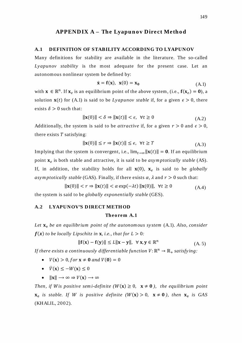
149

APPENDIX A – The Lyapunov Direct Method

A.1 DEFINITION OF STABILITY ACCORDING TO LYAPUNOV

Many definitions for stability are available in the literature. The so-called

Lyapunov stability is the most adequate for the present case. Let an

autonomous nonlinear system be defined by:

�̇� = 𝐟(𝐱), 𝐱(0) = 𝐱𝟎 (A.1) with 𝐱 ∈ ℝ𝑛. If 𝐱𝑒 is an equilibrium point of the above system, (i.e., 𝐟(𝐱𝑒) = 𝟎), a

solution 𝐱(𝑡) for (A.1) is said to be Lyapunov stable if, for a given 𝜖 > 0, there

exists 𝛿 > 0 such that:

‖𝐱(0)‖ < 𝛿 ⇒ ‖𝐱(𝑡)‖ < 𝜖, ∀𝑡 ≥ 0 (A.2) Additionally, the system is said to be attractive if, for a given 𝑟 > 0 and 𝜖 > 0,

there exists 𝑇 satisfying:

‖𝐱(0)‖ ≤ 𝑟 ⇒ ‖𝐱(𝑡)‖ ≤ 𝜖, ∀𝑡 ≥ 𝑇 (A.3) Implying that the system is convergent, i.e., lim𝑡→∞‖𝐱(𝑡)‖ = 𝟎. If an equilibrium

point 𝐱𝑒 is both stable and attractive, it is said to be asymptotically stable (AS).

If, in addition, the stability holds for all 𝐱(0), 𝐱𝑒 is said to be globally

asymptotically stable (GAS). Finally, if there exists 𝛼, 𝜆 and 𝑟 > 0 such that:

‖𝐱(0)‖ < 𝑟 ⇒ ‖𝐱(𝑡)‖ < 𝛼 exp(−𝜆𝑡) ‖𝐱(0)‖, ∀𝑡 ≥ 0 (A.4) the system is said to be globally exponentially stable (GES).

A.2 LYAPUNOV’S DIRECT METHOD

Theorem A.1

Let 𝐱e be an equilibrium point of the autonomous system (A.1). Also, consider

𝒇(𝒙) to be locally Lipschitz in 𝐱, i.e., that for 𝐿 > 0:

‖𝐟(𝐱) − 𝐟(𝐲)‖ ≤ 𝐿‖𝐱 − 𝐲‖, ∀ 𝐱, 𝐲 ∈ ℝ𝑛 (A. 5) If there exists a continuously differentiable function 𝑉:ℝ𝑛 → ℝ+ satisfying:

• 𝑉(𝐱) > 0,𝑓𝑜𝑟 𝐱 ≠ 𝟎 𝑎𝑛𝑑 𝑉(𝟎) = 0

• �̇�(𝐱) ≤ −𝑊(𝐱) ≤ 0

• ‖𝐱‖ ⟶ ∞ ⇒ 𝑉(𝐱) ⟶∞

Then, if 𝑊is positive semi-definite (𝑊(𝐱) ≥ 0, 𝐱 ≠ 𝟎 ), the equilibrium point

𝐱e is stable. If 𝑊 is positive definite (𝑊(𝐱) > 0, 𝐱 ≠ 𝟎 ), then 𝐱e is GAS

(KHALIL, 2002).

Documents

MODELING AND ANALYSIS OF TWO ALTERNATIVES FOR …