Modeling and Applications of Spatial Frequency Domain Imaging (SFDI)

David Cuccia, Ph.DFounder and CEO – Modulated Imaging, Inc.

OutlineIntroduction – Modulated Imaging, Inc.

Spatial Frequency Domain Imaging (SFDI)

Instrumentation

Spectral Imaging

Tomography

Computational Challenges in SFDI

Spatial Frequency Optimization

Wavelength Optimization

Profilometry

Tomographic Imaging

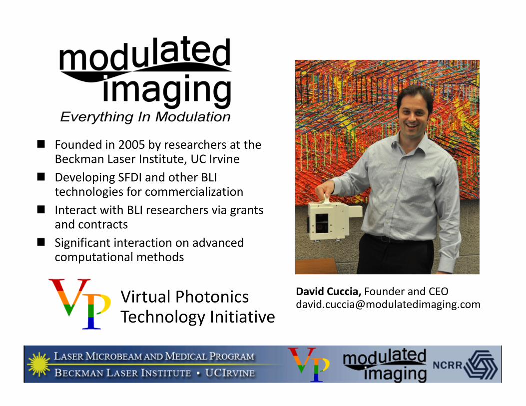
David Cuccia, Founder and CEOdavid.cuccia@modulatedimaging.com

Virtual Photonics Technology Initiative

Founded in 2005 by researchers at the Beckman Laser Institute, UC Irvine

Developing SFDI and other BLI technologies for commercialization

Interact with BLI researchers via grants and contracts

Significant interaction on advanced computational methods

Acknowledgements

Vasan Venugopalan

Jerome Spanier

Carole Hayakawa

Lisa Malenfant

Adam Garnder

Michele Martinelli

Janaka Ranasinghesagara

VP

Frederic Bevilacqua

Anthony Durkin

Bernard Choi

Bruce Tromberg

Ron Frostig

Gregory Evans

Soren Konecky

Amaan Mazhar

Rolf Saager

Amr Yafi

Michael Pharaon

SFDI Lab

NCRR: P41 RR 001192 NCRR: R43 RR 025985-01

Steve Saggese

Pierre Khoury

Frederick Ayers

MI Inc.

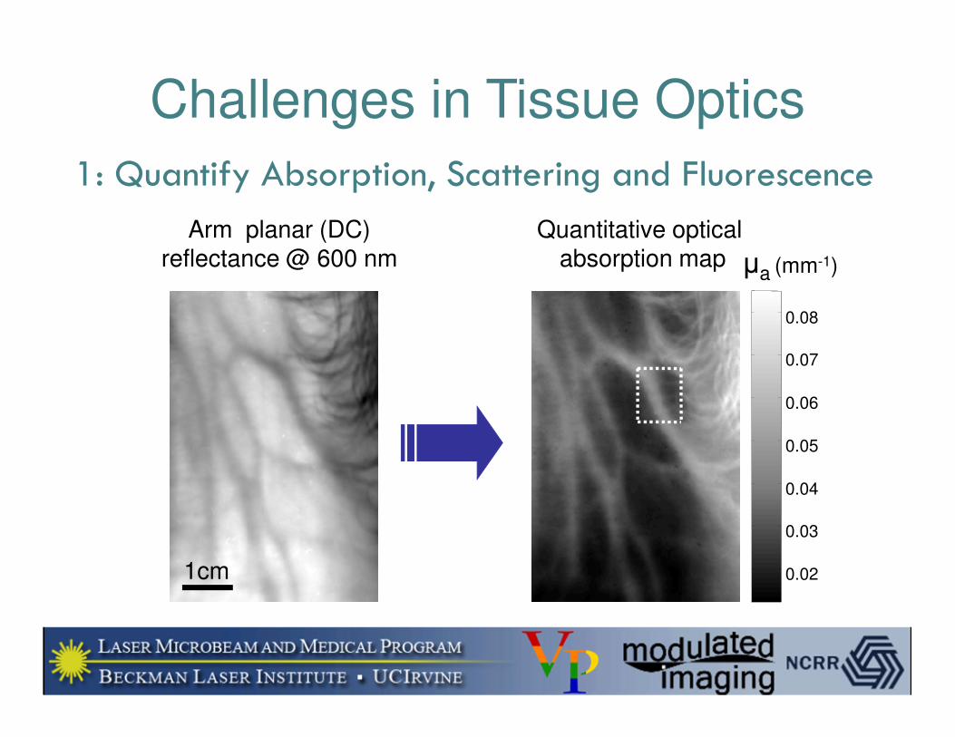
1: Quantify Absorption, Scattering and Fluorescence

Arm planar (DC)reflectance @ 600 nm

1cm 0.02

0.03

0.04

0.05

0.06

0.07

0.08

Quantitative optical absorption map µa (mm-1)

Challenges in Tissue Optics

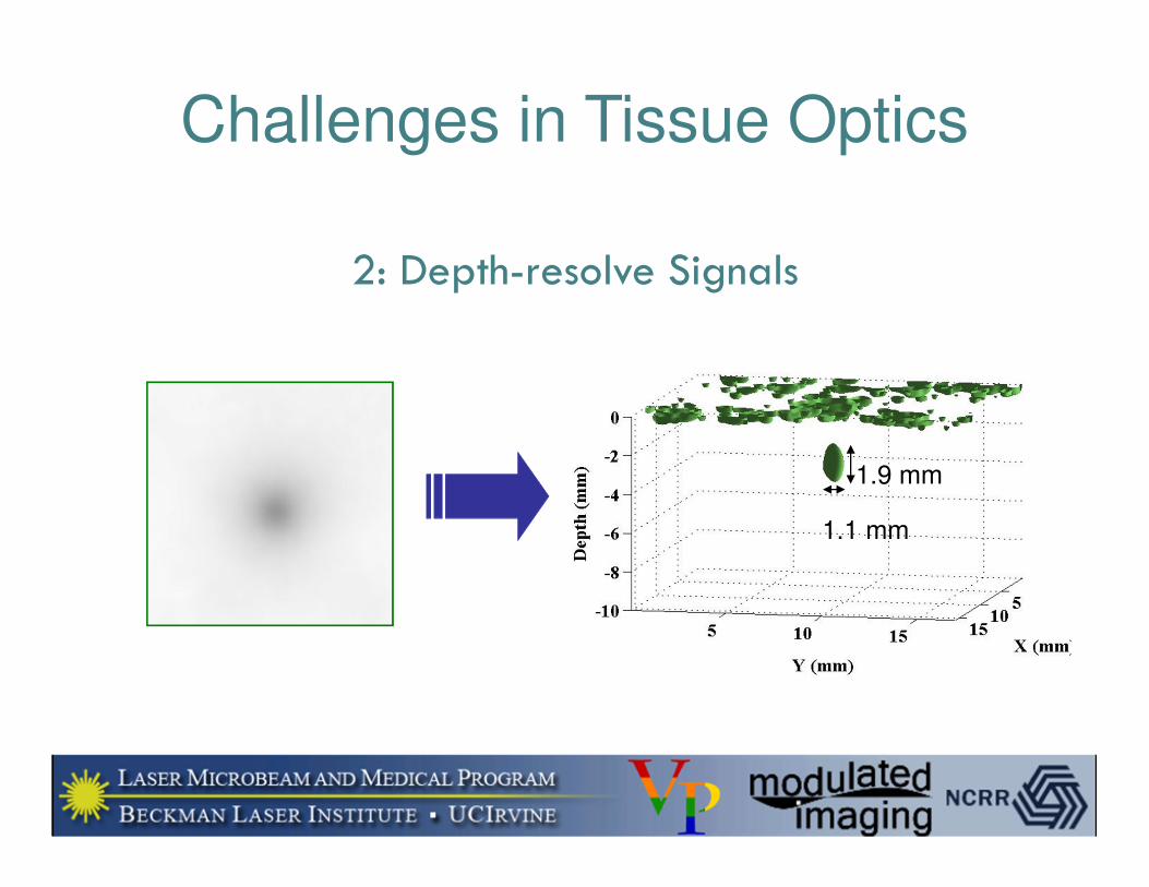
2: Depth-resolve Signals

1.9 mm

1.1 mm

Challenges in Tissue Optics

Structured Illumination Measurement and SFD Modeling in Turbid Media

Nora Dognitz and Georges Wagnieres, Lasers Med. Sci. 13, 55 (1998).

Structured Illumination + Spatial Frequency Domain Analysis

M. A. A. Neil, R. Juskaitis, and T. Wilson, Opt. Lett. 22, 19057 (1997).

Spatial Frequency Domain Measurement in Diffractive Systems

David J. Cuccia, Frederic Bevilacqua, Anthony J. Durkin, and Bruce J. Tromberg, "Modulated imaging: quantitative analysis and tomography of turbid media in the spatial-frequency domain," Opt. Lett. 30, 1354-1356 (2005)

Spatial Frequency Domain Measurement and Analysis

X. Cheng and D. A. Boas, Opt. Express 3, 118 (1998)

Markel, V. and Schotland, J. J. Opt. Soc. Am. A 18, 1336-1347 (2001)

Spatial Frequency Domain Modeling in Turbid Media

Alwin Kienle, Michael S. Patterson, Nora Dögnitz, Roland Bays, Georges Wagnieres, and Hubert van den Bergh. Appl. Opt. 37, 779-791 (1998)

Fre

quency D

om

ain

Real D

om

ain

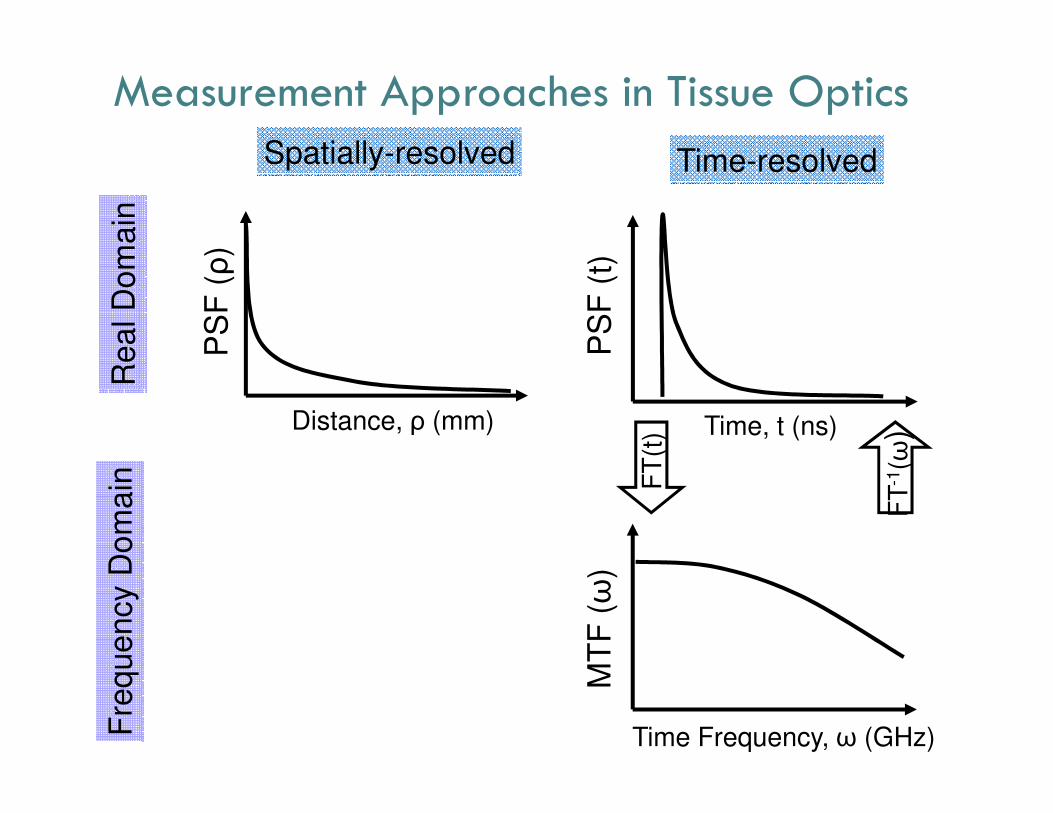
FT

(t)

FT

-1(ω

)

MT

F (ω

)

Time Frequency, ω (GHz)

PS

F (

t)

Time, t (ns)

Time-resolved

PS

F (ρ

)

Distance, ρ (mm)

Spatially-resolved

Measurement Approaches in Tissue Optics

Fre

quency D

om

ain

Real D

om

ain

FT

(t)

FT

-1(ω

)

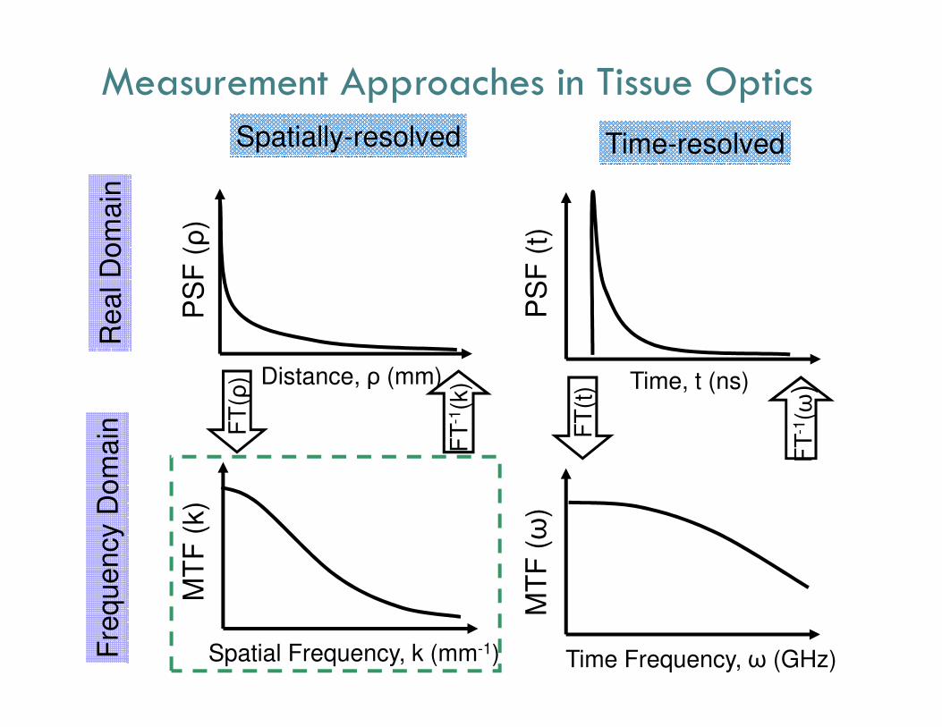
MT

F (ω

)

Time Frequency, ω (GHz)

PS

F (

t)

Time, t (ns)

Time-resolved

MT

F (

k)

Spatial Frequency, k (mm-1)

FT

(ρ)

FT

-1(k

)

PS

F (ρ

)

Distance, ρ (mm)

Spatially-resolved

Measurement Approaches in Tissue Optics

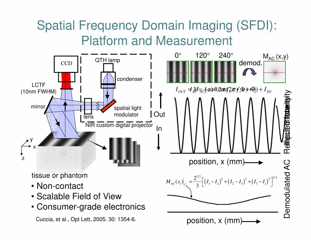
Spatial Frequency Domain Imaging (SFDI):

Platform and Measurement

x

z

y

lens

mirror

LCTF(10nm FWHM)

condenser

QTH lamp

spatial light modulator

NIR custom digital projector

tissue or phantom

CCD

Re

fle

cte

d In

ten

sity

position, x (mm)

( ) ( ) ( )1/ 2 1/ 2

2 2 2

1 2 2 3 3 1

2( )

3xiAC i f

M x I I I I I I = − + − + −

De

mo

du

late

d A

C

( )*cos(2 )OUT AC x DCI M x f x Iπ= + Φ +

0Φ = 2 / 3πΦ = 4 / 3πΦ =

Out

In

1 12 2cos(2 )IN xI f xπ= + Φ +

Inp

ut In

ten

sity

position, x (mm)

demod.MAC (x,y)240°120°0°

• Non-contact

• Scalable Field of View

• Consumer-grade electronics

Cuccia, et al., Opt Lett, 2005. 30: 1354-6.

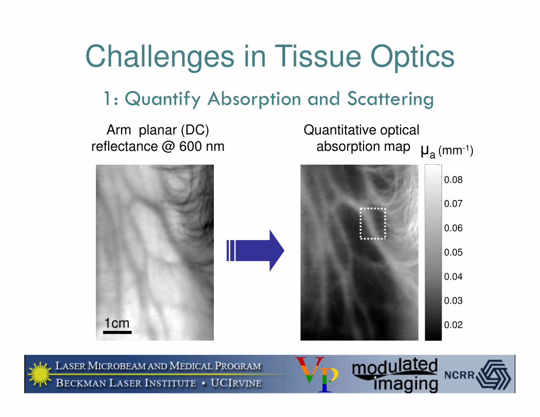
1: Quantify Absorption and Scattering

Arm planar (DC)reflectance @ 600 nm

1cm 0.02

0.03

0.04

0.05

0.06

0.07

0.08

Quantitative optical absorption map µa (mm-1)

Challenges in Tissue Optics

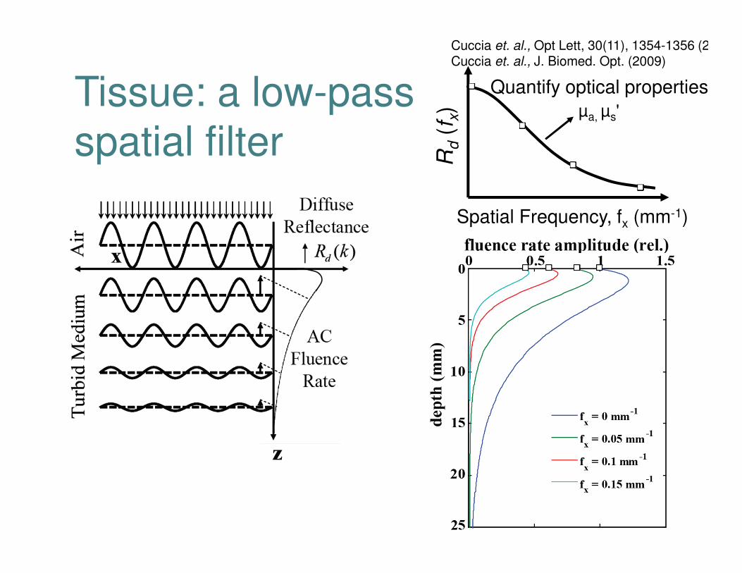
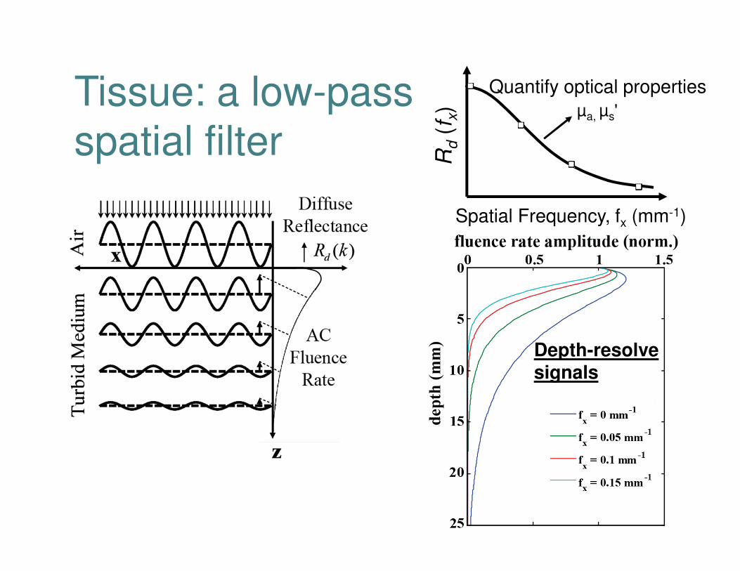
Tissue: a low-pass spatial filter R

d(f

x)

Spatial Frequency, fx (mm-1)

µa, µs'

Cuccia et. al., Opt Lett, 30(11), 1354-1356 (2005)Cuccia et. al., J. Biomed. Opt. (2009)

Quantify optical properties

0

1

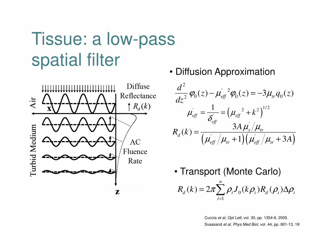
( ) 2 ( ) ( )n

d i i d i i

i

R k J k Rπ ρ ρ ρ ρ=

= ∆∑

( ) ( )

'

' '

3( )

1 3

s trd

eff tr eff tr

AR k

A

µ µ

µ µ µ µ=

+ +

( )1/ 2

' 2 2

'

1eff eff

eff

kµ µδ

= = +

2' 2

0 0 02( ) ( ) 3 ( )

eff tr

dz z q z

dzϕ µ ϕ µ− = −

• Diffusion Approximation

• Transport (Monte Carlo)

Tissue: a low-pass spatial filter

Cuccia et al, Opt Lett, vol. 30, pp. 1354-6, 2005.

Svaasand et al, Phys Med Biol, vol. 44, pp. 801-13, 1999.

0 0.05 0.1 0.15 0.2 0.25 0.30

0.1

0.2

0.3

0.4

0.5

0.6

0.7

0.8

Spatial frequency (mm-1

)

Dif

fuse

Refl

ecta

nce

0 0.05 0.1 0.15 0.2 0.25 0.30

0.1

0.2

0.3

0.4

0.5

0.6

0.7

0.8

Spatial frequency (mm-1

)

Dif

fuse

Ref

lect

an

ce

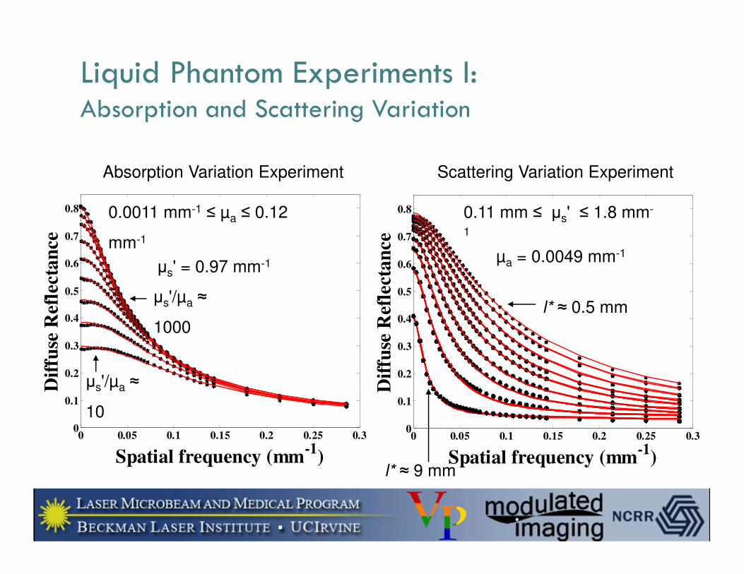
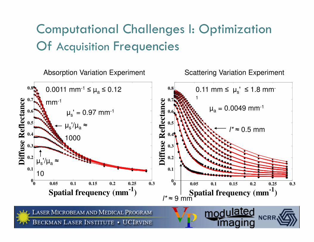
Liquid Phantom Experiments I:Absorption and Scattering Variation

Absorption Variation Experiment Scattering Variation Experiment

0.11 mm ≤ µs' ≤ 1.8 mm-

1

µa = 0.0049 mm-1

0.0011 mm-1 ≤ µa ≤ 0.12

mm-1

µs' = 0.97 mm-1

µs'/µa ≈

10

µs'/µa ≈

1000l* ≈ 0.5 mm

l* ≈ 9 mm

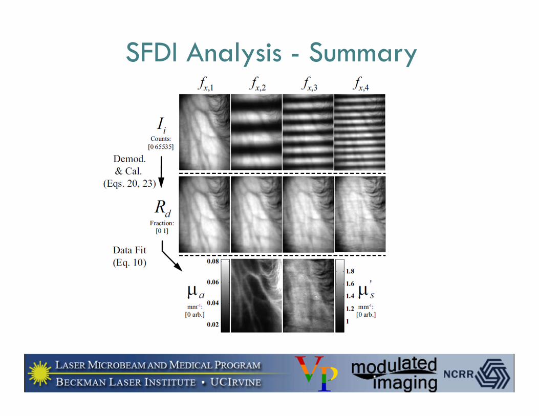
SFDI Analysis - Summary

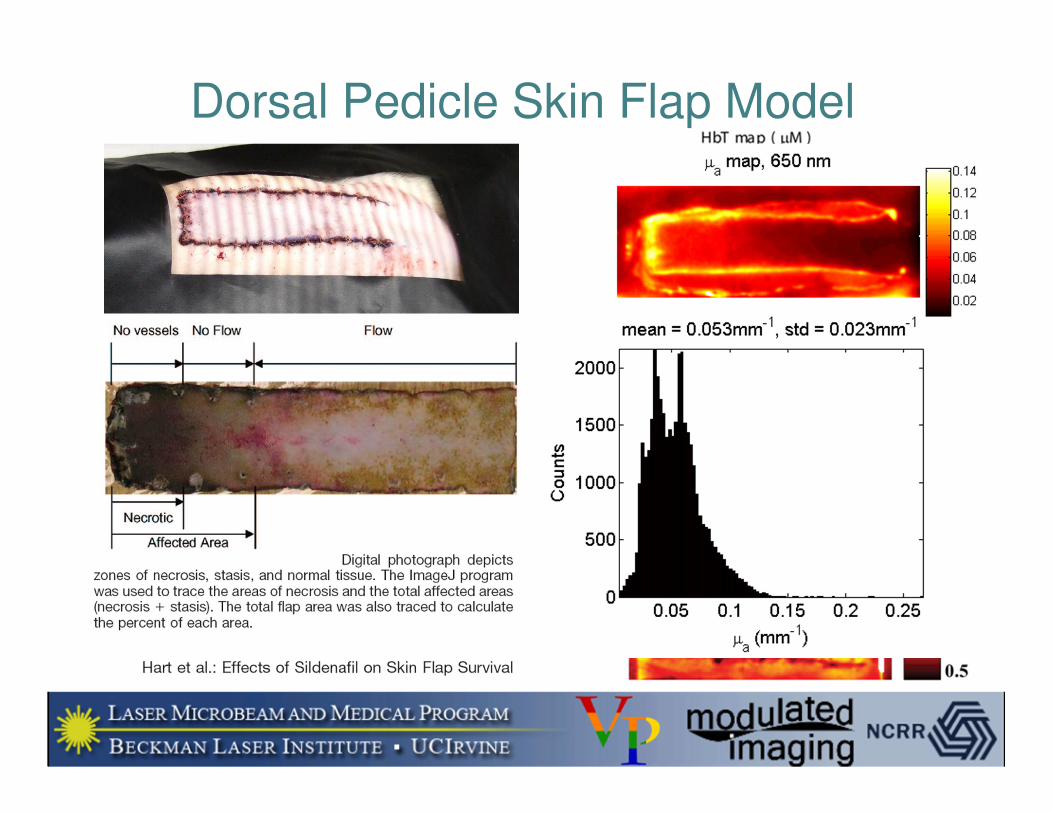
Dorsal Pedicle Skin Flap Model

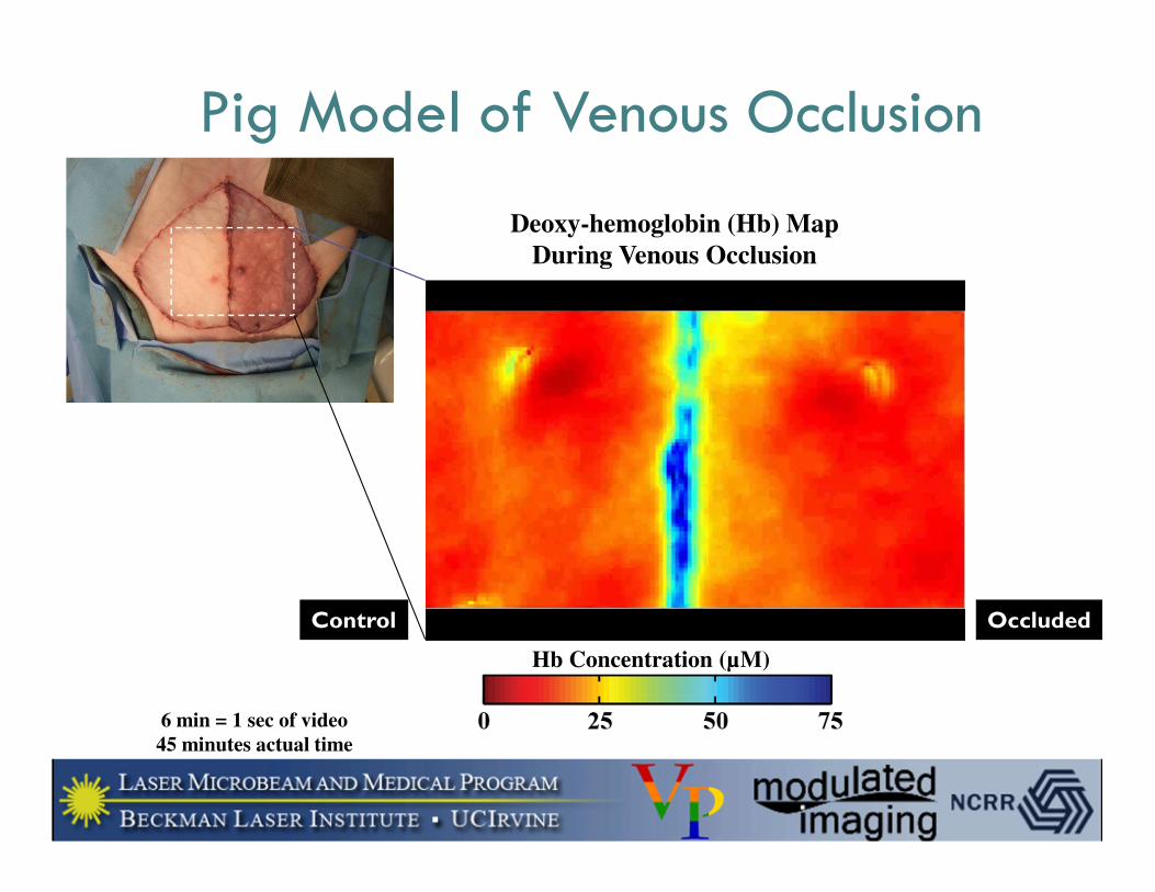
Pig Model of Venous Occlusion

Deoxy-hemoglobin (Hb) Map

During Venous Occlusion

Control Occluded

6 min = 1 sec of video

45 minutes actual time

Hb Concentration (µM)

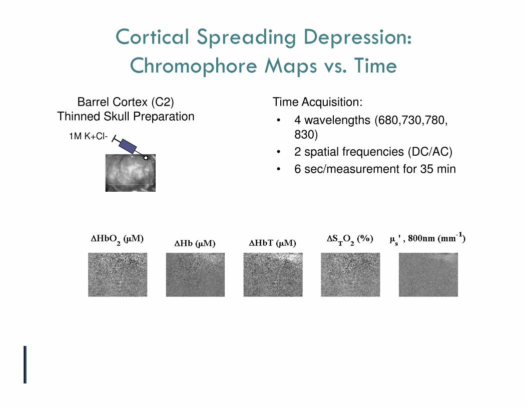
Cortical Spreading Depression:Chromophore Maps vs. Time

Barrel Cortex (C2)Thinned Skull Preparation

1M K+Cl-

• 4 wavelengths (680,730,780, 830)

• 2 spatial frequencies (DC/AC)

• 6 sec/measurement for 35 min

Time Acquisition:

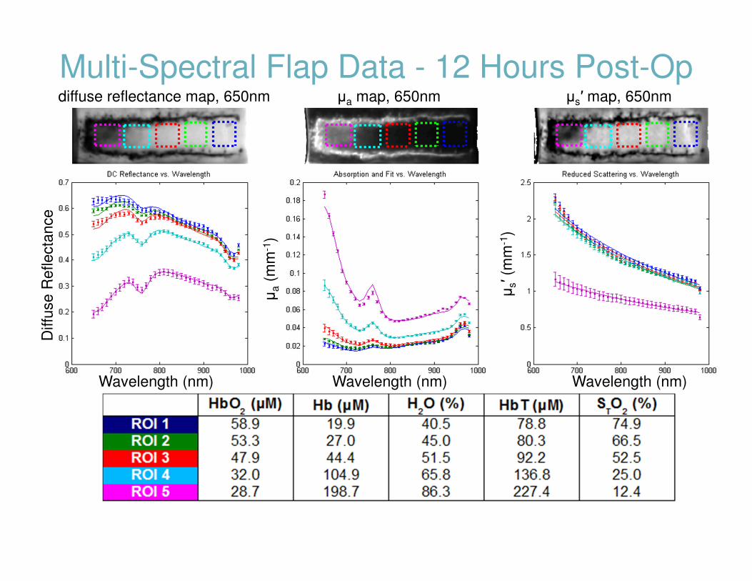
Multi-Spectral Flap Data - 12 Hours Post-Op

µa

(mm

-1)

µs′(m

m-1

)

Diffu

se

Re

fle

cta

nce

Wavelength (nm) Wavelength (nm) Wavelength (nm)

µa map, 650nm µs′ map, 650nmdiffuse reflectance map, 650nm

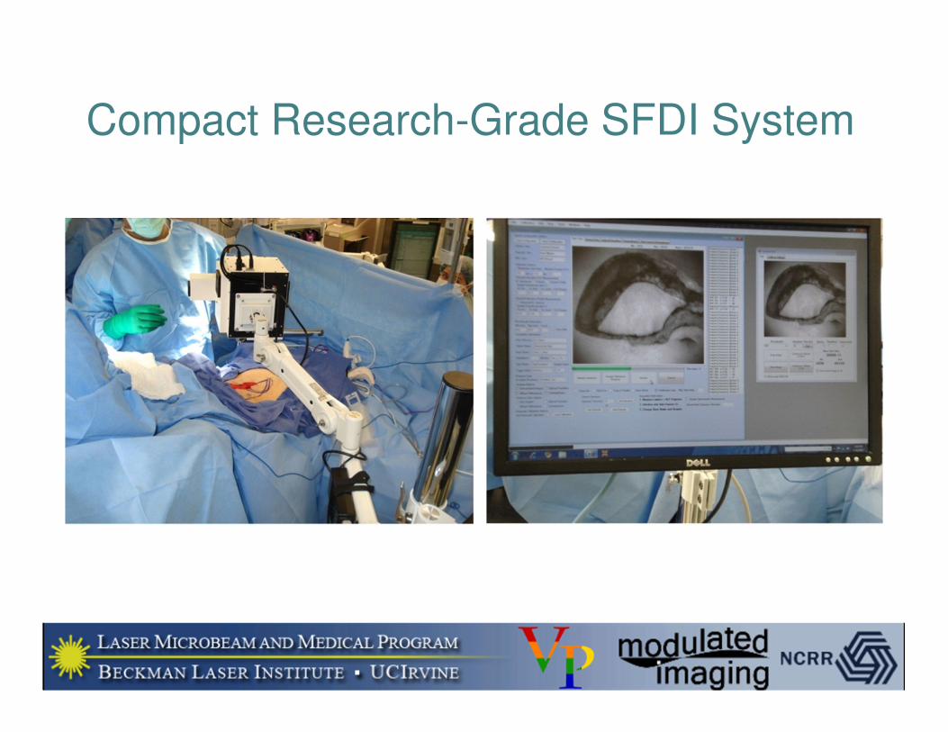
Compact Research-Grade SFDI System

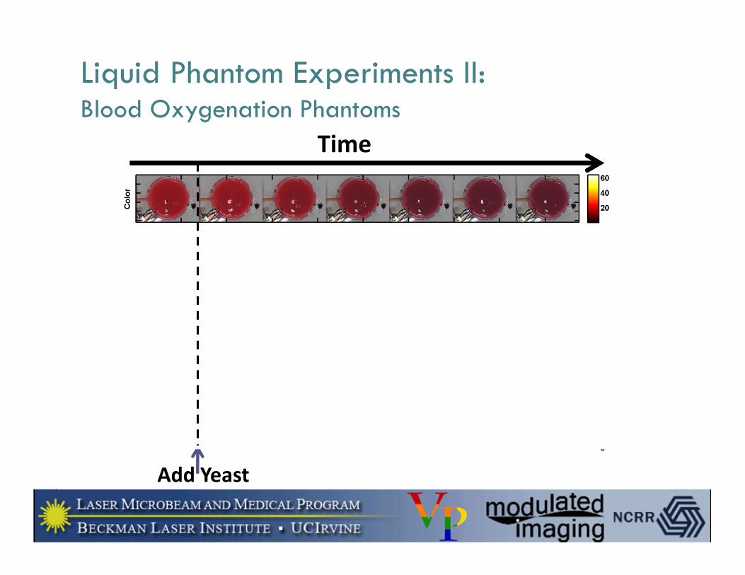
Liquid Phantom Experiments II:Blood Oxygenation Phantoms

Add Yeast

Time

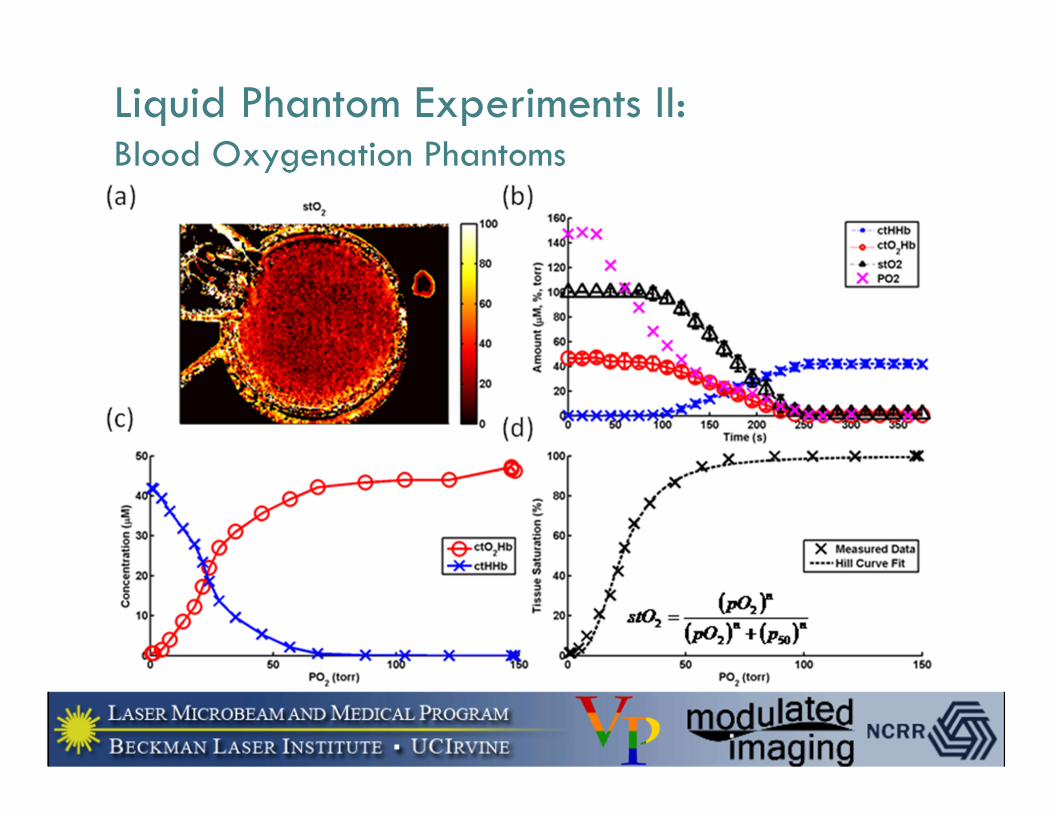
Liquid Phantom Experiments II:Blood Oxygenation Phantoms

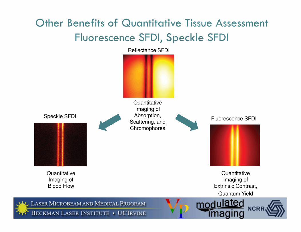
Other Benefits of Quantitative Tissue Assessment Fluorescence SFDI, Speckle SFDI

Reflectance SFDI

Quantitative Imaging of Absorption,

Scattering, and Chromophores

Speckle SFDI

Quantitative Imaging of Blood Flow

Fluorescence SFDI

Quantitative Imaging of

Extrinsic Contrast,

Quantum Yield

0 0.05 0.1 0.15 0.2 0.25 0.30

0.1

0.2

0.3

0.4

0.5

0.6

0.7

0.8

Spatial frequency (mm-1

)

Dif

fuse

Refl

ecta

nce

0 0.05 0.1 0.15 0.2 0.25 0.30

0.1

0.2

0.3

0.4

0.5

0.6

0.7

0.8

Spatial frequency (mm-1

)

Dif

fuse

Ref

lect

an

ce

Absorption Variation Experiment Scattering Variation Experiment

0.11 mm ≤ µs' ≤ 1.8 mm-

1

µa = 0.0049 mm-1

0.0011 mm-1 ≤ µa ≤ 0.12

mm-1

µs' = 0.97 mm-1

µs'/µa ≈

10

µs'/µa ≈

1000l* ≈ 0.5 mm

l* ≈ 9 mm

Computational Challenges I: Optimization Of Acquisition Frequencies

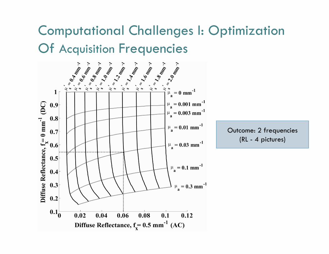
Computational Challenges I: Optimization Of Acquisition Frequencies

Outcome: 2 frequencies(RL - 4 pictures)

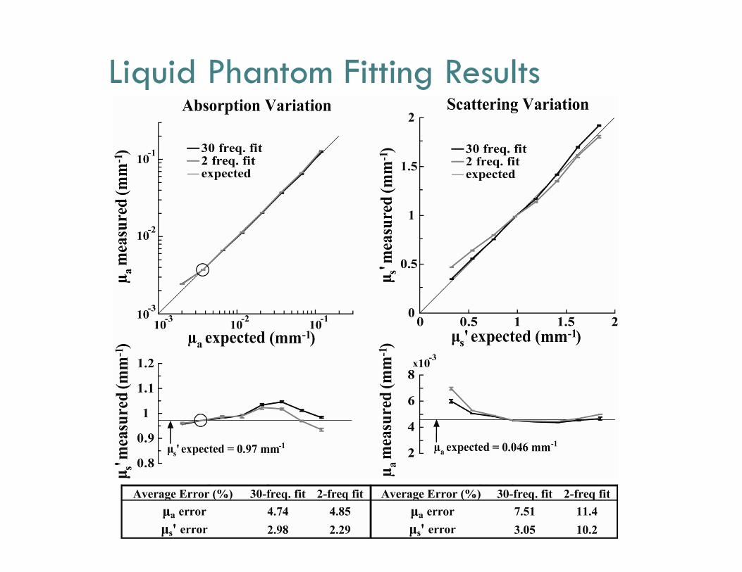
Liquid Phantom Fitting Results

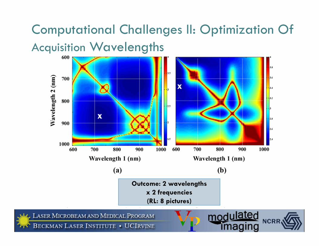
Computational Challenges II: Optimization Of Acquisition Wavelengths

Outcome: 2 wavelengths

x 2 frequencies

(RL: 8 pictures)

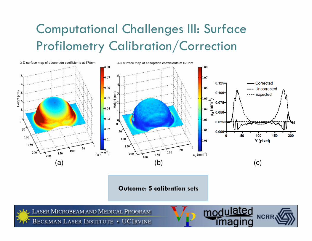
MI-derived 670nm absorption maps of a homogeneous hemispherical tissue phantom without (a) and with (b) profile-based reflectance calibration. (c) Corresponding absorption line profiles.

(a) (b) (c)

Computational Challenges III: Surface Profilometry Calibration/Correction

Outcome: 5 calibration sets

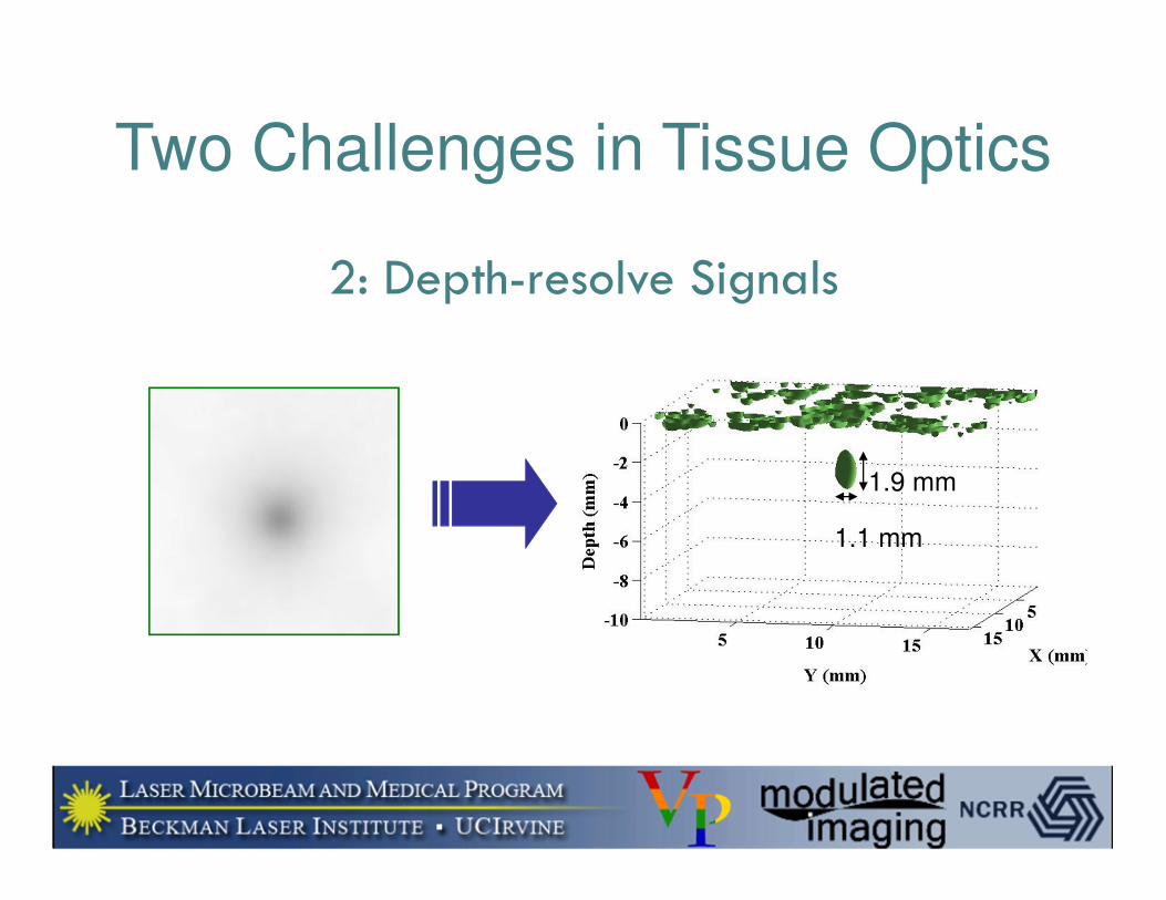
2: Depth-resolve Signals

1.9 mm

1.1 mm

Two Challenges in Tissue Optics

Tissue: a low-pass spatial filter R

d(f

x)

Spatial Frequency, fx (mm-1)

µa, µs'

Depth-resolvesignals

Quantify optical properties

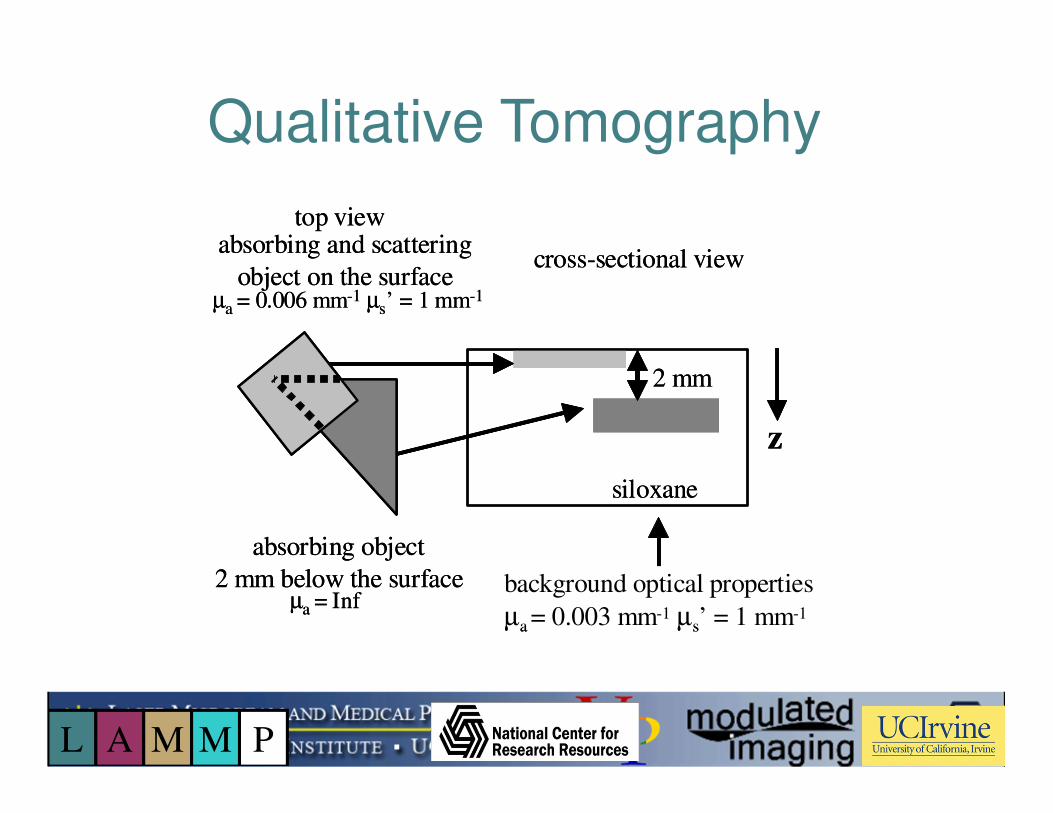
absorbing object

2 mm below the surface

absorbing and scattering

object on the surface

2 mm

z

top view

cross-sectional view

siloxane

µa = 0.006 mm-1 µs’ = 1 mm-1

µa = Infbackground optical properties

µa = 0.003 mm-1 µs’ = 1 mm-1

absorbing object

2 mm below the surface

absorbing and scattering

object on the surface

2 mm

z

top view

cross-sectional view

siloxane

µa = 0.006 mm-1 µs’ = 1 mm-1

µa = Infbackground optical properties

µa = 0.003 mm-1 µs’ = 1 mm-1

Qualitative Tomography

L A M M P

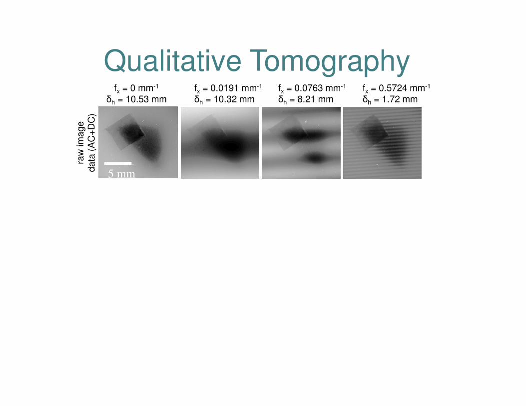
raw

im

age

data

(A

C+

DC

)

modula

tion

images

derivative

sections

fx = 0 mm-1

δh = 10.53 mmfx = 0.0191 mm-1

δh = 10.32 mmfx = 0.0763 mm-1

δh = 8.21 mmfx = 0.5724 mm-1

δh = 1.72 mm

5 mm5 mm

Qualitative Tomography

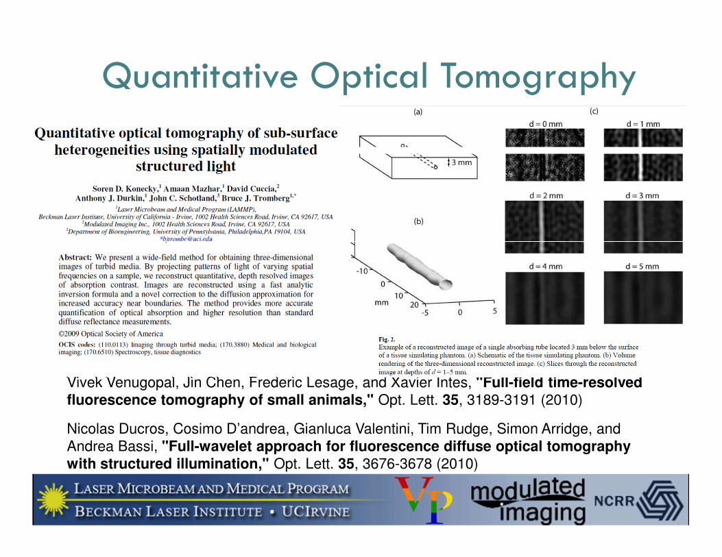
Vivek Venugopal, Jin Chen, Frederic Lesage, and Xavier Intes, "Full-field time-resolved

fluorescence tomography of small animals," Opt. Lett. 35, 3189-3191 (2010)

Nicolas Ducros, Cosimo D’andrea, Gianluca Valentini, Tim Rudge, Simon Arridge, and

Andrea Bassi, "Full-wavelet approach for fluorescence diffuse optical tomography

with structured illumination," Opt. Lett. 35, 3676-3678 (2010)

Quantitative Optical Tomography

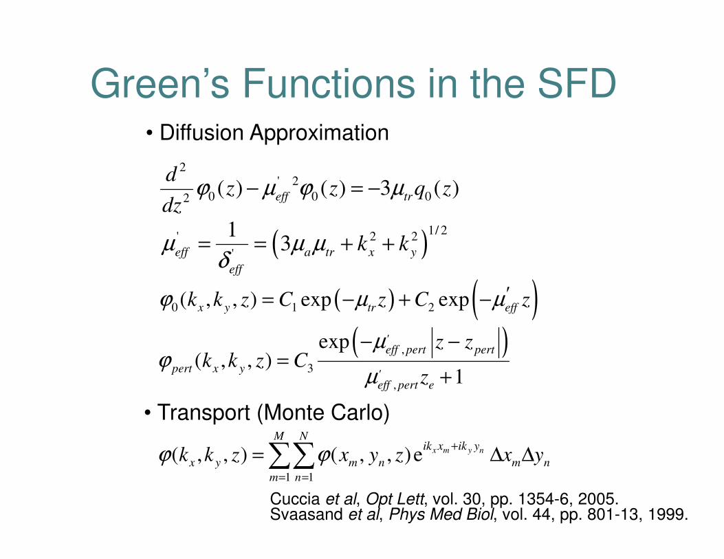
1 1

( , , ) ( , , )e x m y n

M Nik x ik y

x y m n m n

m n

k k z x y z x yϕ ϕ+

= =

= ∆ ∆∑∑

( )1/ 2

' 2 2

'

13eff a tr x y

eff

k kµ µ µδ

= = + +

2' 2

0 0 02( ) ( ) 3 ( )eff tr

dz z q z

dzϕ µ ϕ µ− = −

• Diffusion Approximation

• Transport (Monte Carlo)

Cuccia et al, Opt Lett, vol. 30, pp. 1354-6, 2005.Svaasand et al, Phys Med Biol, vol. 44, pp. 801-13, 1999.

( ) ( )0 1 2( , , ) exp expx y tr eff'k k z C z C zϕ µ µ= − + −

Green’s Functions in the SFD

( ),

3

,

exp( , , )

1

'eff pert pert

pert x y'eff pert e

z zk k z C

z

µϕ

µ

− −=

+

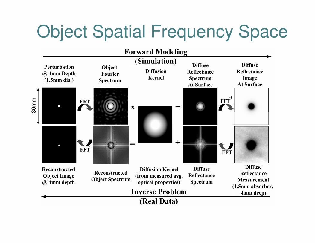
30m

mObject Spatial Frequency Space

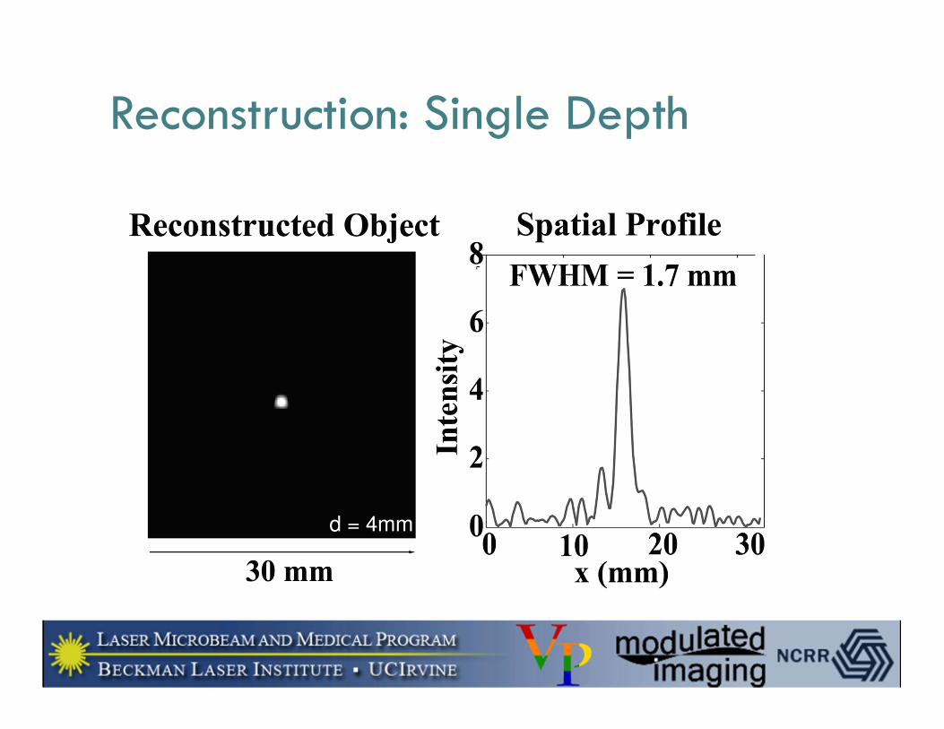
d = 4mm

Reconstruction: Single Depth

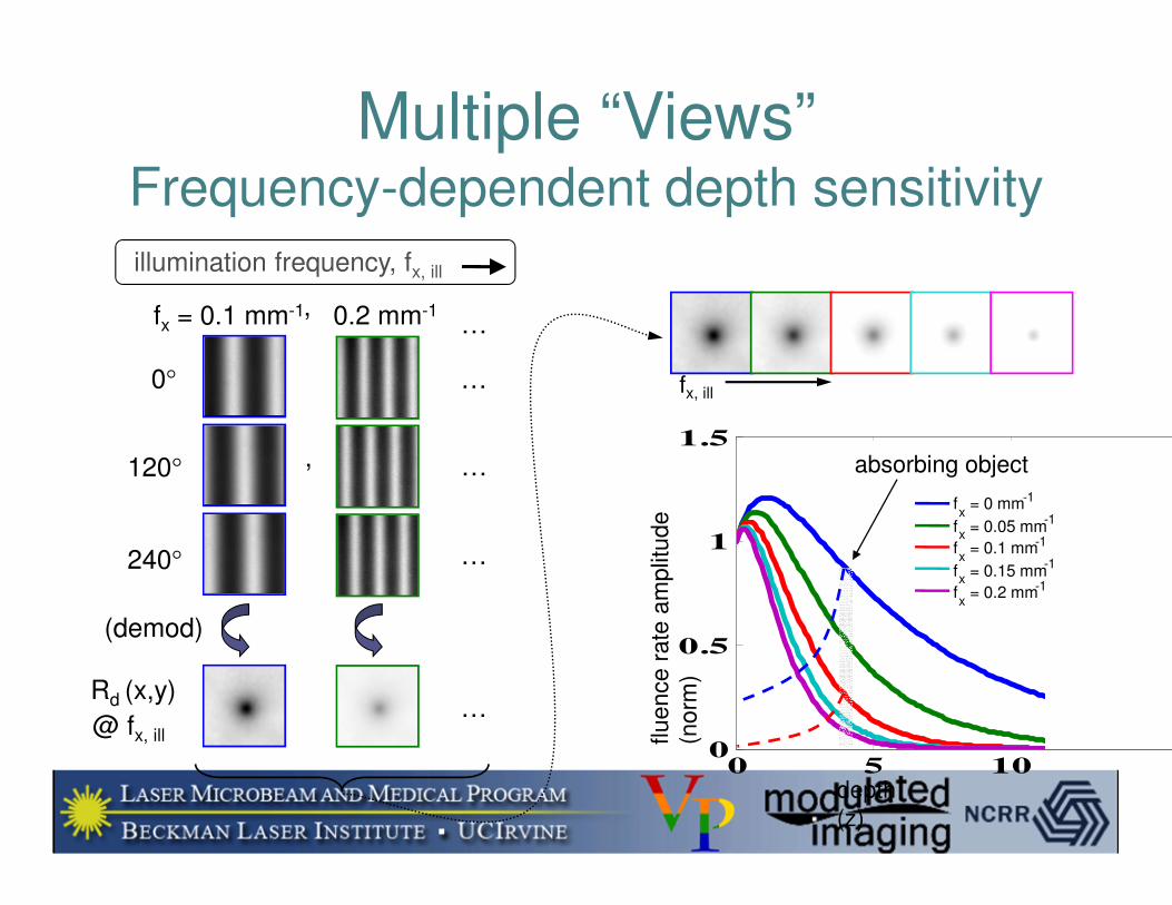
0 5 100

0.5

1

1.5

flu

en

ce

ra

te a

mp

litu

de

(no

rm)

depth

(z)

fx

= 0 mm-1

fx

= 0.05 mm-1

fx

= 0.1 mm-1

fx

= 0.15 mm-1

fx

= 0.2 mm-1

(demod)

240°

120°

0°

fx = 0.1 mm-1

Rd (x,y)

@ fx, ill

Multiple “Views”Frequency-dependent depth sensitivity

illumination frequency, fx, ill

, 0.2 mm-1

, …

…

…

…

… fx, ill

absorbing object

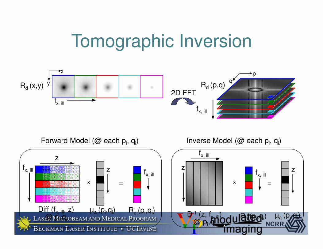
2D FFT

fx, ill

Rd (p,q)

p

qRd (x,y)

z

=

µa (pi,qi)

z

x

fx, ill fx, ill

Rd (pi,qi)Diff (fx, ill, z)@ pi,qi

Tomographic Inversion

Forward Model (@ each pi, qi)

z

=x

fx, ill

fx, ill

Rd (pi,qi)D-1 (z, fx, ill)

@ pi,qi

µa (pi,qi)

z

Inverse Model (@ each pi, qi)

fx, ill

x

y

d = 4mm

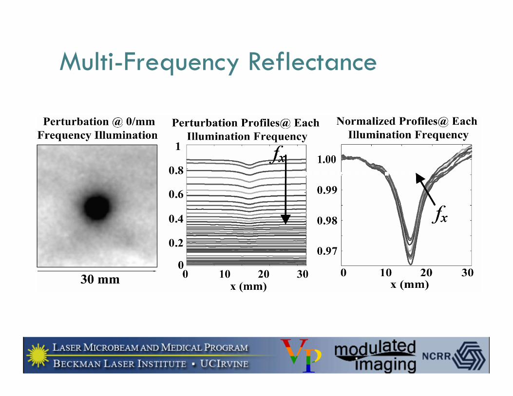
Multi-Frequency Reflectance

1.9 mm

1.1 mm

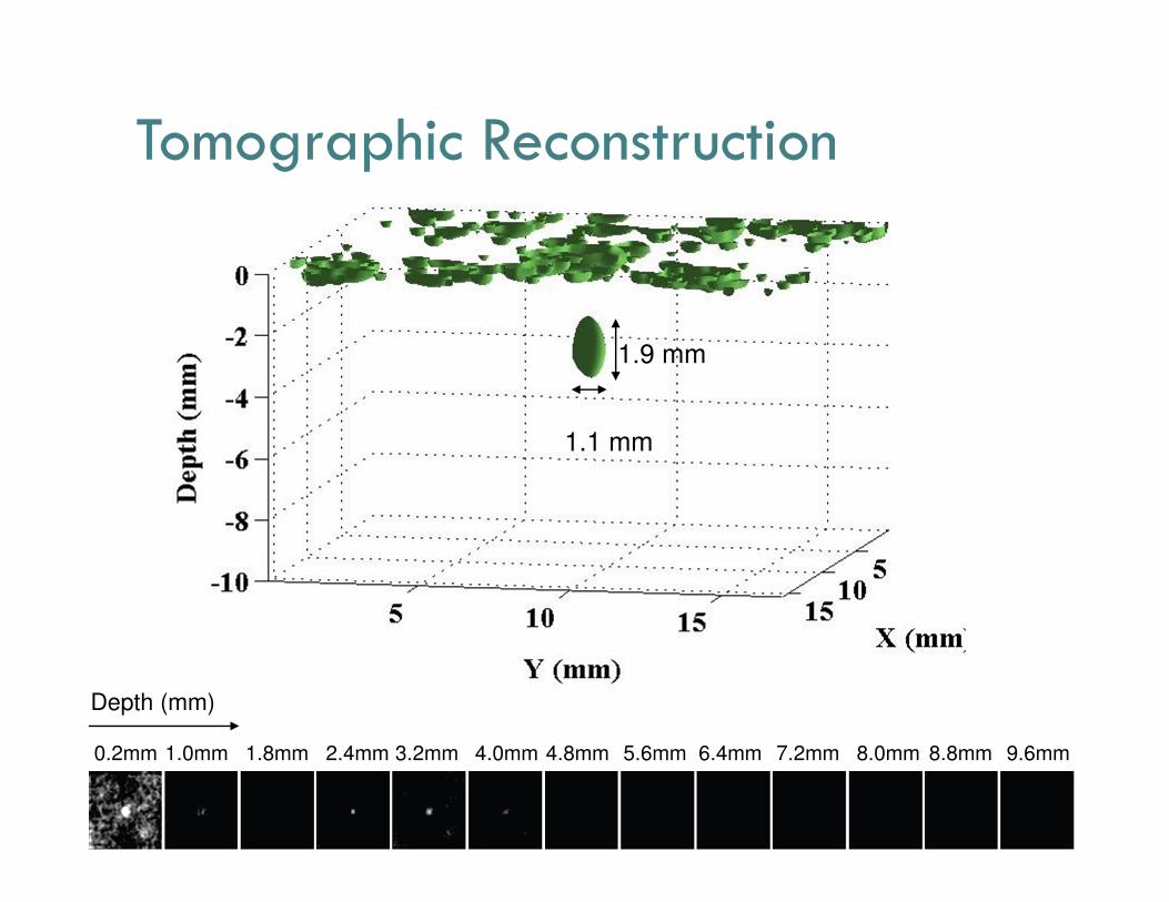
Tomographic Reconstruction

0.2mm 1.0mm 1.8mm 2.4mm 3.2mm 4.0mm 4.8mm 5.6mm 6.4mm 7.2mm 8.0mm 8.8mm 9.6mm

Depth (mm)

Ongoing Work

Clinical Deployment

Multi-modality imaging (laser speckle, fluorescence)

Advanced modeling (acceleration, layers, tomography)

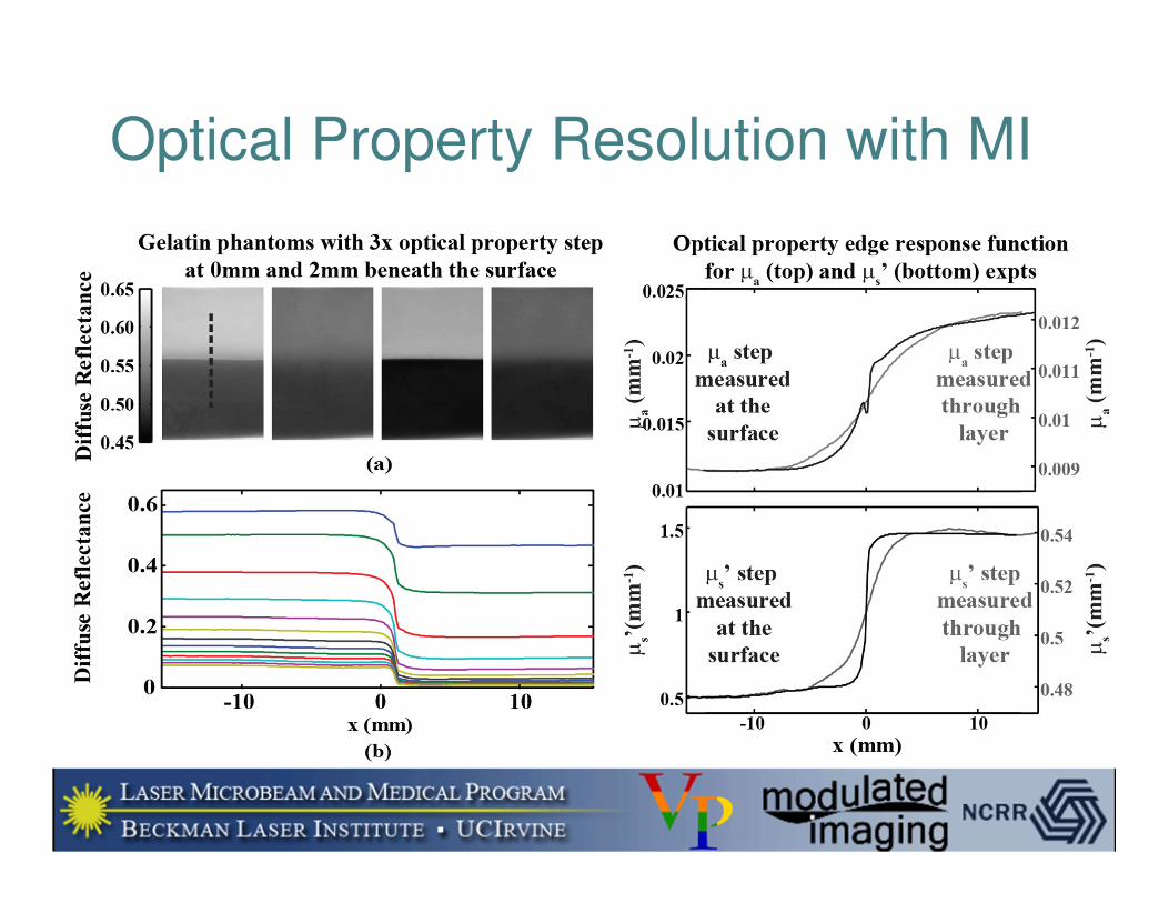
Optical Property Resolution with MI